15.835: Entrepreneurial Marketing

Session 6Demand Forecasting

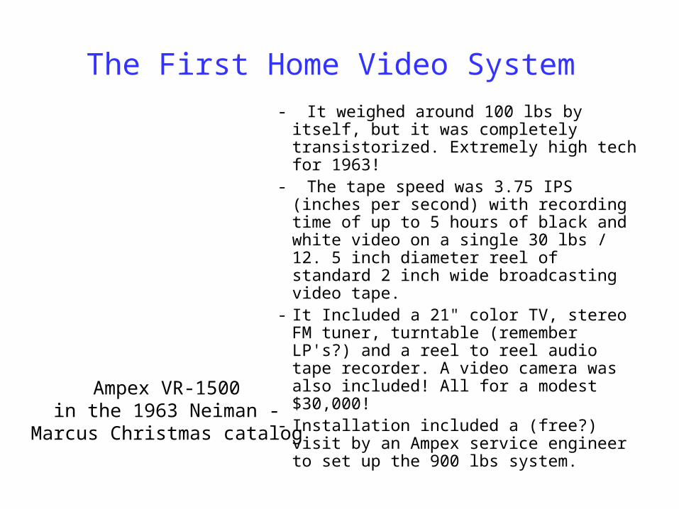
The First Home Video System - It weighed around 100 lbs by itself, but

it was completely transistorized. Extremely high tech for 1963!

- The tape speed was 3.75 IPS (inches per second) with recording time of up to 5 hours of black and white video on a single 30 lbs / 12. 5 inch diameter reel of standard 2 inch wide broadcasting video tape.

- It Included a 21" color TV, stereo FM tuner, turntable (remember LP's?) and a reel to reel audio tape recorder. A video camera was also included! All for a modest $30,000!

- Installation included a (free?) visit by an Ampex service engineer to set up the 900 lbs system.

Ampex VR-1500in the 1963 Neiman -

Marcus Christmas catalog

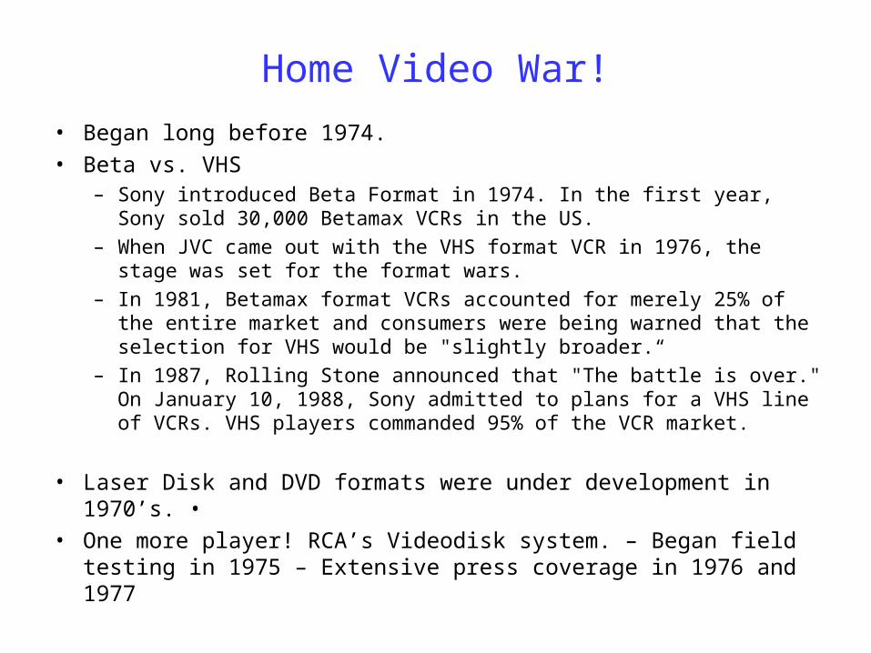
Home Video War!• Began long before 1974. • Beta vs. VHS

– Sony introduced Beta Format in 1974. In the first year, Sony sold 30,000 Betamax VCRs in the US.

– When JVC came out with the VHS format VCR in 1976, the stage was set for the format wars.

– In 1981, Betamax format VCRs accounted for merely 25% of the entire market and consumers were being warned that the selection for VHS would be "slightly broader.“

– In 1987, Rolling Stone announced that "The battle is over." On January 10, 1988, Sony admitted to plans for a VHS line of VCRs. VHS players commanded 95% of the VCR market.

• Laser Disk and DVD formats were under development in 1970’s. •• One more player! RCA’s Videodisk system. – Began field testing in

1975 – Extensive press coverage in 1976 and 1977

RCA Selecta Videodisk Player

– Medium: CED (Capacitance Electronic Discs), housed in 16” housing case – Used a needle to read disc surface – One sounded: cartridge must be flipped over half way through the movie – No recording function

RCA Selecta Videodisk Player (cont’d)

• Demand Forecasting – Conducted market research – Expected to sell 200,000 players and 2 million disks in 1981 – Forecasted that in 10 years the players would be in 30% to 50% of all

American households with $7.5 billion in annual sales of players and discs.

“Our customer for video discs is clearly the average family, the same broad segment that built the television business to 1980's level of nearly 16 million annual unit sales." (Ack K. Sauter, RCA vice president)

“Video disc players will reach a higher sales level in the first year than any other major video product in the history of the industry." (Sauter)

What They Did?

• Value Proposition: “Easy to use, depth of software, and affordability”

• Allies: Zenith, JC Penney, Sears, Sanyo, Toshiba, Hitachi, and Radio Shack

• 5000 retail outlets • $22 Million Advertising • Initial Price

$499.95 for the player $14.98 to $39.98 for CED disc titles.

What Happened?

• Sold 100,000 players, half of the forecasted sales, in 1981 – When the system hit the market, VCR's were well established – Typical consumers thought "Why would I want this VideoDisc

player, when for about the same price I can get a VCR that both plays and records.“

– RCA's market research didn't take videocassette rental into account at all, and a lot of consumers who earlier would have been willing to purchase movies now preferred to rent them.

• Cum. Sales in 1984: 500,000 Units

• Withdrew in 1986 – Loss: $580 Million

What We Learn from Videodisk?

• The importance of Demand Forecasting

– Business feasibility assessment • Is the market potential big enough?

– Decision on resource commitment before market launch

– Pricing

Demand Forecasting of an Innovative Product/Service

• What is the challenge of it?

– No historical data • Time-series methods are inapplicable

Topics

• How to forecast sales of a truly innovative product/service

• How to forecast sales of an early entrant to market • How to forecast sales of a pioneer brand after the

market entry of a new competitor

Part I. How to forecast sales of a truly innovative product/service

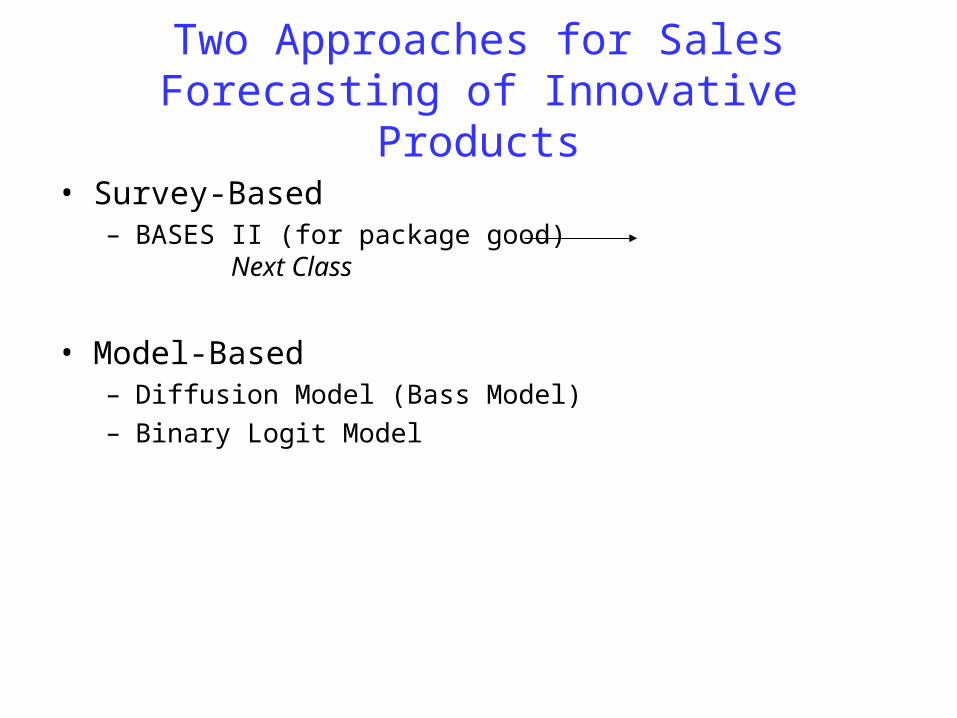
Two Approaches for Sales Forecasting of Innovative Products

• Survey-Based – BASES II (for package good) Next Class

• Model-Based – Diffusion Model (Bass Model) – Binary Logit Model

A. Diffusion Model (The Bass Model)

The Objective of Diffusion Models

• To represent a life-cycle sales curve of an innovation-a new product or service-among a given set of prospective adopters over time with a small number of parameters.

Assumptions of Diffusion Models

• Applicable to a new product category not to a new brand.

• Each adopter purchases only one unit of the new product – No repeat purchases – Applicable only to durable goods

• Total potential market size is fixed.

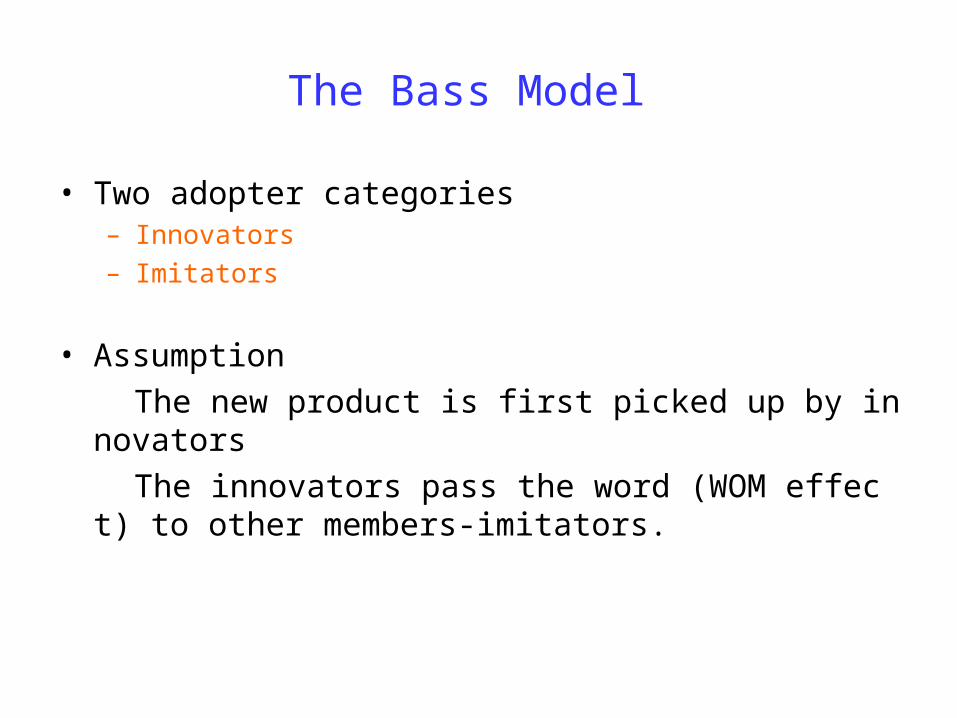
The Bass Model

• Two adopter categories – Innovators – Imitators

• Assumption The new product is first picked up by innovators The innovators pass the word (WOM effect) to other me

mbers-imitators.

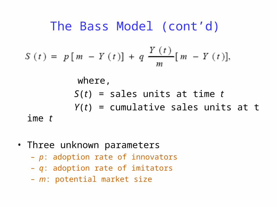
The Bass Model (cont’d)

where, S(t) = sales units at time t Y(t) = cumulative sales units at time t

• Three unknown parameters – p: adoption rate of innovators – q: adoption rate of imitators – m: potential market size

Estimation of the Bass Model

Rewrite as

Run a regression analysis to find a, b, and c. Then, find

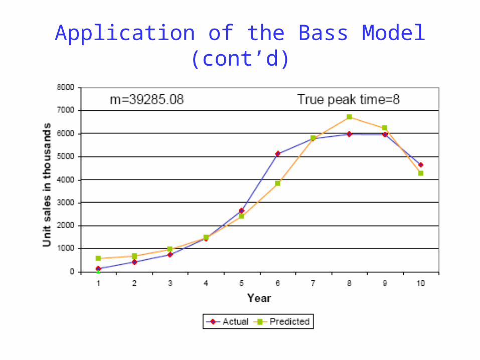
Application of the Bass Model (cont’d)

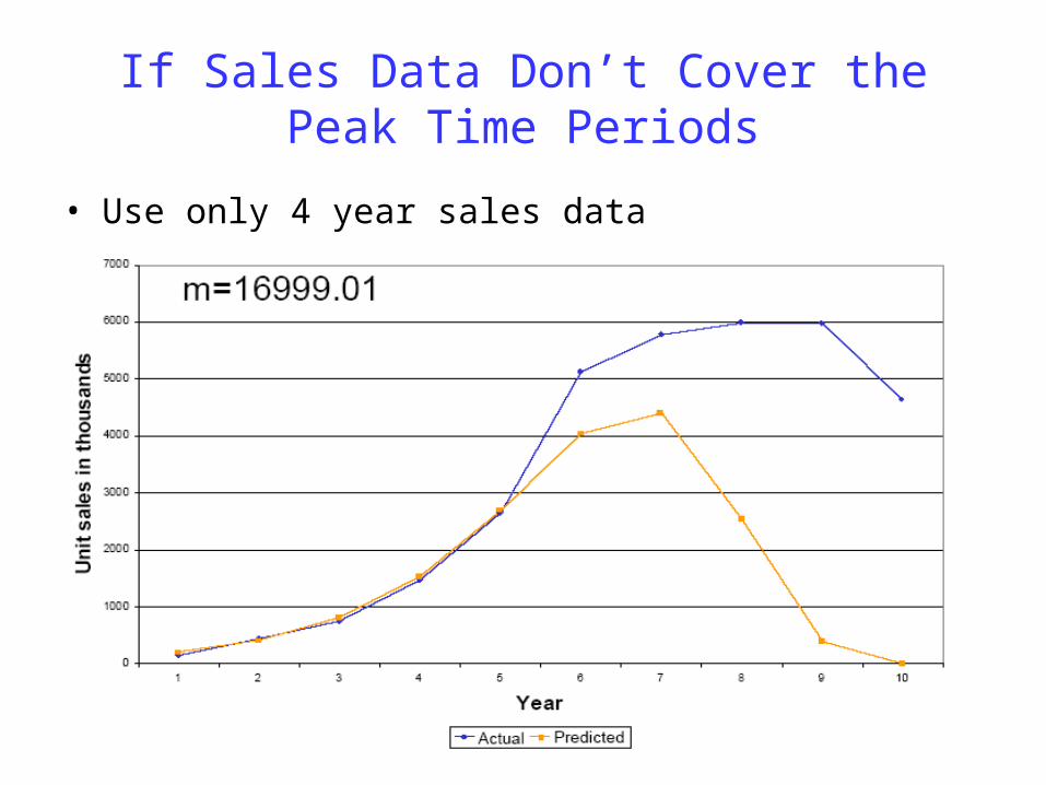
If Sales Data Don’t Cover the Peak Time Periods

• Use only 4 year sales data

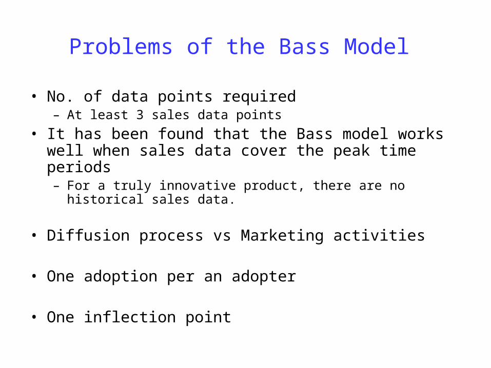
Problems of the Bass Model

• No. of data points required – At least 3 sales data points

• It has been found that the Bass model works well when sales data cover the peak time periods – For a truly innovative product, there are no historical sales data.

• Diffusion process vs Marketing activities

• One adoption per an adopter

• One inflection point

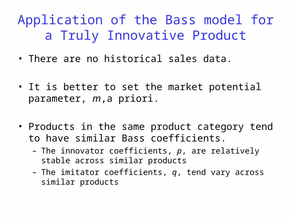
Application of the Bass model for a Truly Innovative Product

• There are no historical sales data.

• It is better to set the market potential parameter, m,a priori.

• Products in the same product category tend to have similar Bass coefficients. – The innovator coefficients, p, are relatively stable across similar

products – The imitator coefficients, q, tend vary across similar products

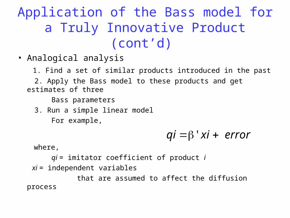
Application of the Bass model for a Truly Innovative Product (cont’d)

• Analogical analysis 1. Find a set of similar products introduced in the past 2. Apply the Bass model to these products and get estimates of three Bass parameters 3. Run a simple linear model For example,

qi β'xi error where, qi = imitator coefficient of product i xi = independent variables that are assumed to affect the diffusion process

Examples of xi

• Similarity ratings • Product evaluation scores • Attribute ratings • Marketing mix variables

• Any variables that are assumed to affect the diffusion process

I-B.Binary Logit Model

Demand Analysis in Binary Logit Model

• Choice or trial intent observations For consumer i (i=1,…,I), yi = 0/1 (No/Yes)

• Then, Total demand=Σiyi

• Therefore, the key is how to predict yi

• Key assumption: (Expected) Utility Maximization A consumer will buy the product If utility obtained from the product > utility from no purchase

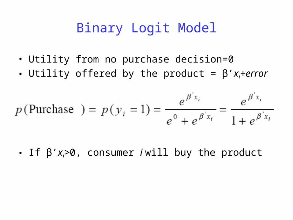
Binary Logit Model

• Utility from no purchase decision=0 • Utility offered by the product = β’xi+error

• If β’xi>0, consumer i will buy the product

Binary Logit Model (cont’d)

• Measurement through survey– yi

• Show the product concept• Ask “Are you likely to buy this product?” (Yes/No)

– Xi

• independent variables that are assumed to affect choice decision

– Product characteristics and/or consumer characteristics – Price term can be included in xi

Part II. Sales Forecasting – When A Start-up firm is an Early Entrant – When Competitors Enter the Market

Multinomial Logit Model

Korean Beer War

• Two Beer Companies, OB and Crown – In 1933, Crown beer was introduced and there were no competit

ors. – In 1948, OB beer was introduced. In 1952, OB beer became a m

arket leader. – Since 1952, OB beer had kept its market leader position for abo

ut 40 years. In 1992, market share of Crown beer was about 15%.

Korean Beer War (cont’d)

• In 1993, Crown beer company introduced a new beer brand, Hite.

– Unique selling proposition: “Freshness”

• OB launched several new beer products (e.g. OB Sound, OB Ice, NEX, CAFRI) but lost their market share quickly.

• To improve revenue structure, OB company decided to enter Korean traditional wine market (Soju), which had been

dominated by a formidable company, Jinro, for about 50 years.

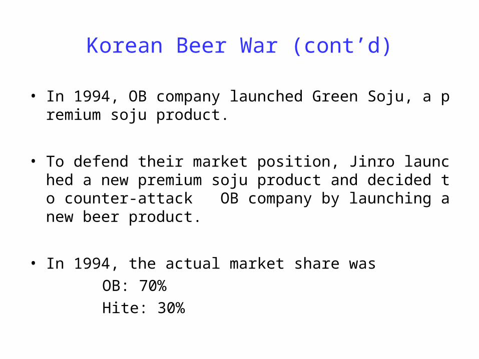
Korean Beer War (cont’d)

• In 1994, OB company launched Green Soju, a premium soju product.

• To defend their market position, Jinro launched a new premium soju product and decided to counter-attack OB company by launching a new beer product.

• In 1994, the actual market share was OB: 70% Hite: 30%

Demand Forecasting for the New Beer

• In 1993, a market survey was conducted.

• After collecting about 3000 questionnaires, the multinomial logit model was applied to forecast market share of Cass.

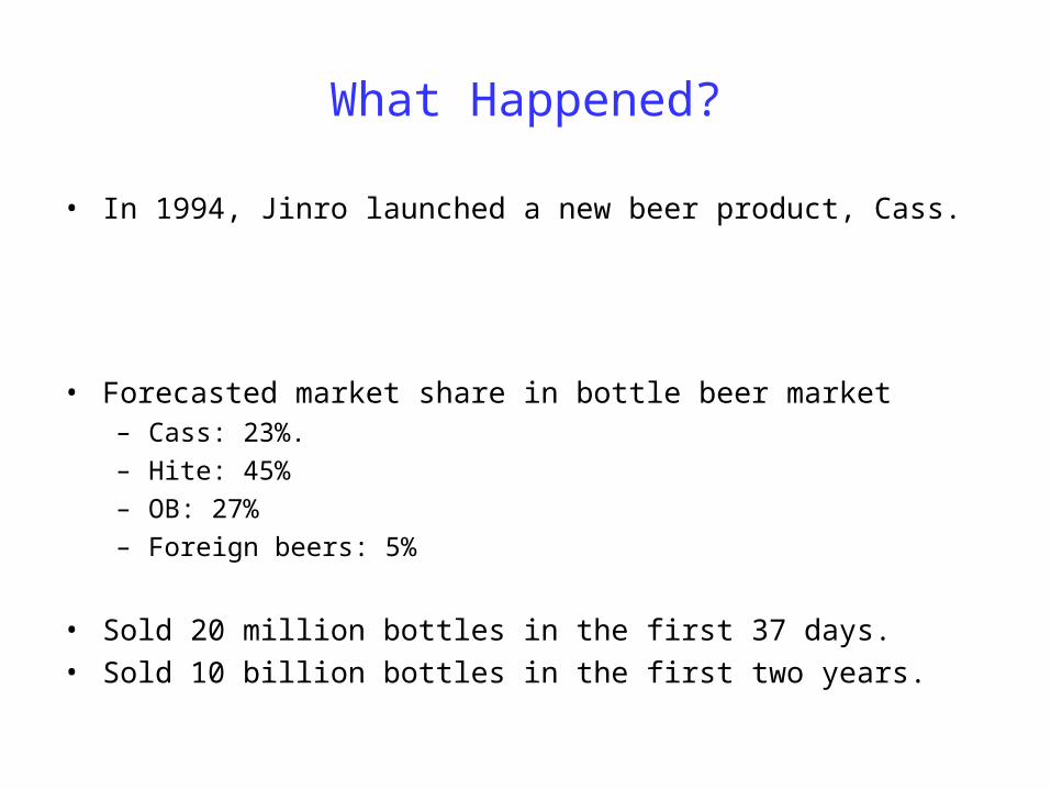
What Happened?

• In 1994, Jinro launched a new beer product, Cass.

• Forecasted market share in bottle beer market – Cass: 23%. – Hite: 45% – OB: 27% – Foreign beers: 5%

• Sold 20 million bottles in the first 37 days. • Sold 10 billion bottles in the first two years.

What is Multinomial Logit Model?

• i: Consumer (i=1,…,I) • j: Choice alternative (j=1,…,J)• Independent variable (xij): vector of explanatory variables for i and j

which are assumed to determine purchase decision (e.g., evaluation on attributes)

• Then, utility of a person for a product is assumed to be a linear model:

Utility of consumer i for product j

What is Multinomial Logit Model? (cont’d)

• Dependent variable (yi) – yi is a polychotomous response, yi {1,…,J}∈

• Then,

(Expected) Utility Maximization Assumption • Assume errors are independently and identically distribut

ed with Weibull distribution, then we have

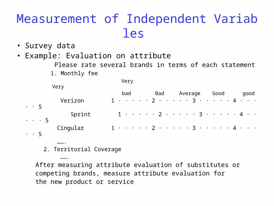
Measurement of Independent Variables • Survey data • Example: Evaluation on attribute Please rate several brands in terms of each statement 1. Monthly fee Very Very bad Bad Average Good good Verizon 1 · · · · · 2 · · · · · 3 · · · · · 4 · · · · · 5 Sprint 1 · · · · · 2 · · · · · 3 · · · · · 4 · · · · · 5 Cingular 1 · · · · · 2 · · · · · 3 · · · · · 4 · · · · · 5 ……. 2. Territorial Coverage ……. After measuring attribute evaluation of substitutes or competing brands, measure attribute evaluation for the new product or service

Measurement of Independent Variables (cont’d)

• It is better if respondents are exposed to a sample of the new product.

• In addition, some marketing decision variables can be entered into xij – Prices, package type, …..

Measurement of Dependent Variable

• “Among all products/brands including the product we described (or showed),

Which product do you want to buy?” • It is possible to measure purchase intension with varyi

ng marketing variables for the new product(e.g., $1, $1.5, …)

Estimation of Logit Model

• Key is to get the estimate of β

• In order to get good estimate of β, the sample size needs to be over 150