15.401 Finance Theory I - MITweb.mit.edu/astomper/www/univie/pof/Chapter 6.pdf · _Brealey, Myers...

Lecture Notes

15.401

15.401 Finance Theory I15.401 Finance Theory I

AlexAlex Stomper StomperMIT Sloan School of ManagementMIT Sloan School of Management

Institute for Advanced Studies, ViennaInstitute for Advanced Studies, Vienna

Lecture 6: OptionsLecture 6: Options

TexPoint fonts used in EMF.Read the TexPoint manual before you delete this box.: AAAAAAAAAAAAAA

Lecture Notes

15.401 Lecture 6: Options

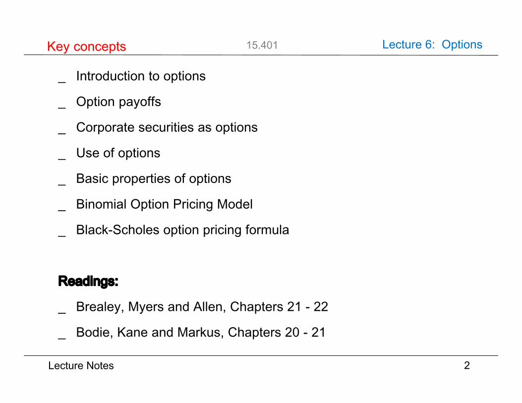
_ Introduction to options

_ Option payoffs

_ Corporate securities as options

_ Use of options

_ Basic properties of options

_ Binomial Option Pricing Model

_ Black-Scholes option pricing formula

Readings:

_ Brealey, Myers and Allen, Chapters 21 - 22

_ Bodie, Kane and Markus, Chapters 20 - 21

2

Key conceptsKey concepts

TexPoint fonts used in EMF.Read the TexPoint manual before you delete this box.: AAAAAAAAAAAAA

Lecture Notes


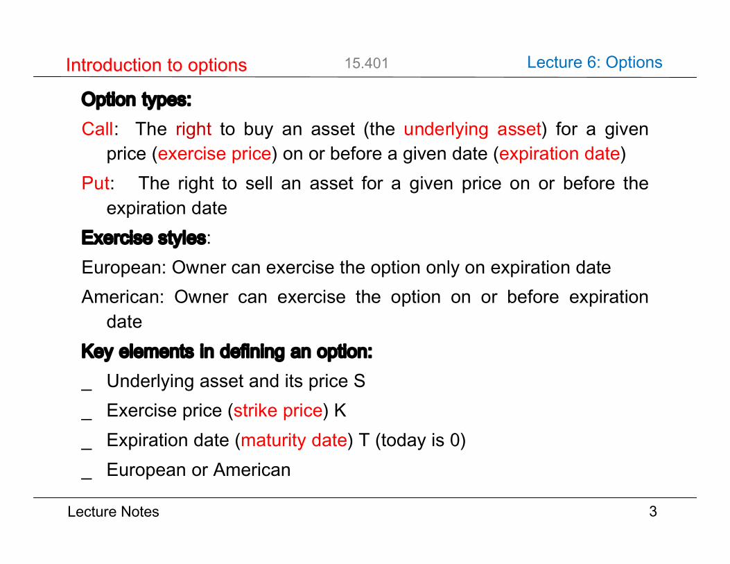
Option types:Call: The right to buy an asset (the underlying asset) for a given

price (exercise price) on or before a given date (expiration date)Put: The right to sell an asset for a given price on or before the

expiration dateExercise styles:European: Owner can exercise the option only on expiration dateAmerican: Owner can exercise the option on or before expiration

dateKey elements in defining an option:_ Underlying asset and its price S_ Exercise price (strike price) K_ Expiration date (maturity date) T (today is 0)_ European or American

3

Introduction to optionsIntroduction to options

Lecture Notes


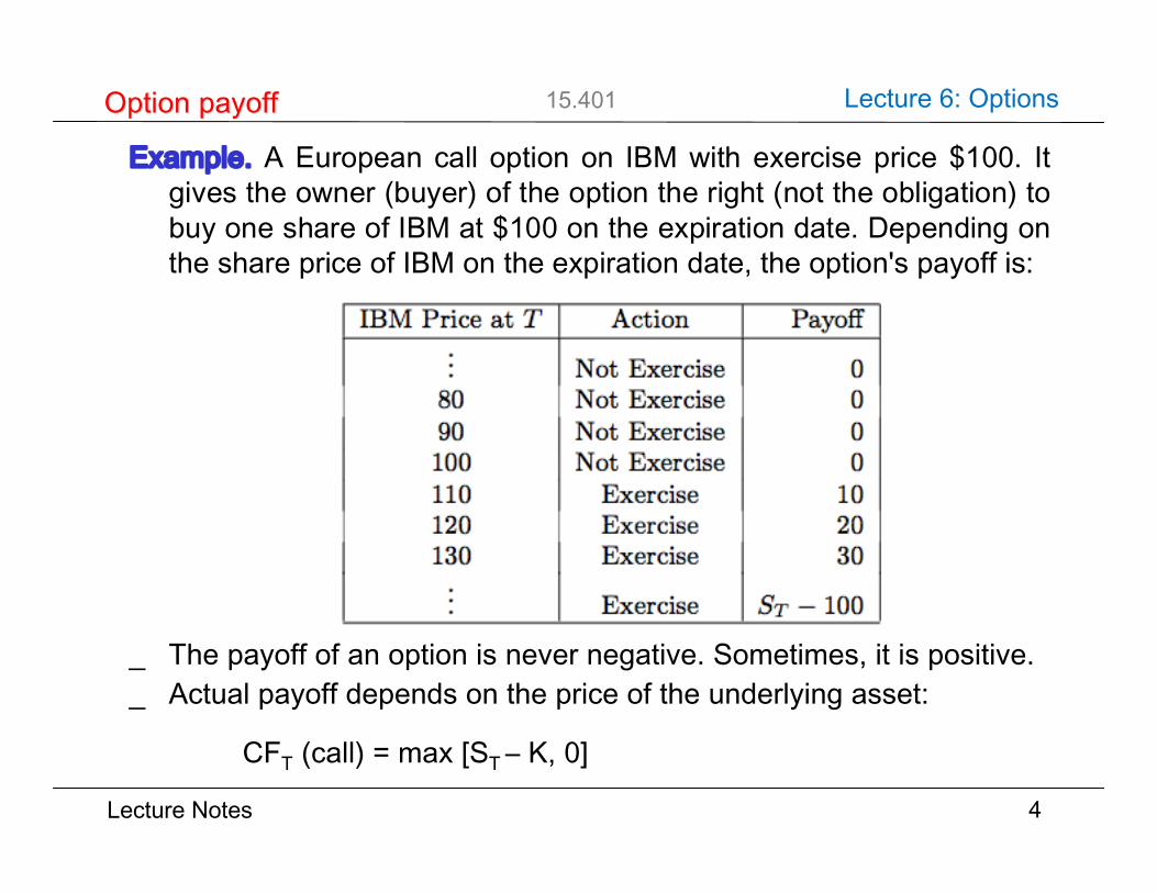
Example. A European call option on IBM with exercise price $100. Itgives the owner (buyer) of the option the right (not the obligation) tobuy one share of IBM at $100 on the expiration date. Depending onthe share price of IBM on the expiration date, the option's payoff is:

_ The payoff of an option is never negative. Sometimes, it is positive._ Actual payoff depends on the price of the underlying asset:

CFT (call) = max [ST ‒ K, 0]

4

Option payoffOption payoff

IBM Price at T Action Payo®... Not Exercise 080 Not Exercise 090 Not Exercise 0100 Not Exercise 0110 Exercise 10120 Exercise 20130 Exercise 30... Exercise ST ¡ 100

Lecture Notes


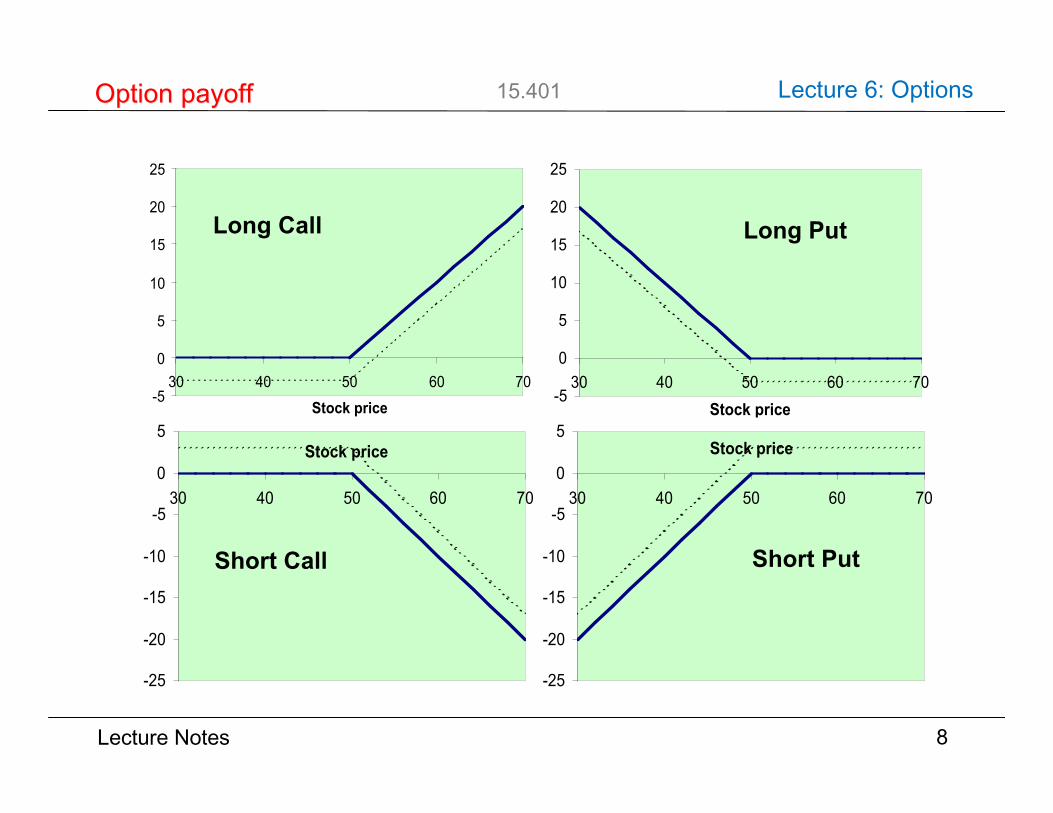
Option payoffs can be plotted as a function of the price of theunderlying asset at expiration:

5


-

6

A ssetpr i ce

P ayoff ofbuy i n ga ca l l

100

100

¡¡¡¡¡

-

6

A ssetpr i ce

P ayoff ofbuy i n ga pu t

100

100

@@

@@@

-

?

A ssetpr i ce

P ayoff of

sel l i n ga ca l l

100

-100

@@@@@

-

?

A ssetpr i ce

P ayoff of

sel l i n ga pu t

100

-100

¡¡

¡¡¡

Lecture Notes


The net payoff from an option must includes its cost.

Example. A European call on IBM shares with an exercise price of$100 and maturity of three months is trading at $5. The 3-monthinterest rate, not annualized, is 0.5%. What is the price of IBM thatmakes the call break-even?

At maturity, the call's net payoff is as follows:

6


IBM Price Action Payo® Net payo®... Not Exercise 0 - 5.02580 Not Exercise 0 - 5.02590 Not Exercise 0 - 5.025100 Not Exercise 0 - 5.025110 Exercise 10 4.975120 Exercise 20 14.975130 Exercise 30 24.975... Exercise ST ¡ 100 ST ¡ 100 ¡ 5.25

Lecture Notes


The break even point is given by:

or7


-

6

Assetprice

Payo®

100

100

-5.0250

a a a a a a a a a a a a a a a a a a aa a a a a a a a a a a a a a a a a a a a

¡¡¡¡

¡¡

¡¡

ST = $105.025

Lecture Notes


8


-5

0

5

10

15

20

25

30 40 50 60 70

Stock price-5

0

5

10

15

20

25

30 40 50 60 70Stock price

-25

-20

-15

-10

-5

0

5

30 40 50 60 70

Stock price

-25

-20

-15

-10

-5

0

5

30 40 50 60 70

Stock price

Long Call

Short Put

Long Put

Short Call

Lecture Notes


9


Lecture Notes


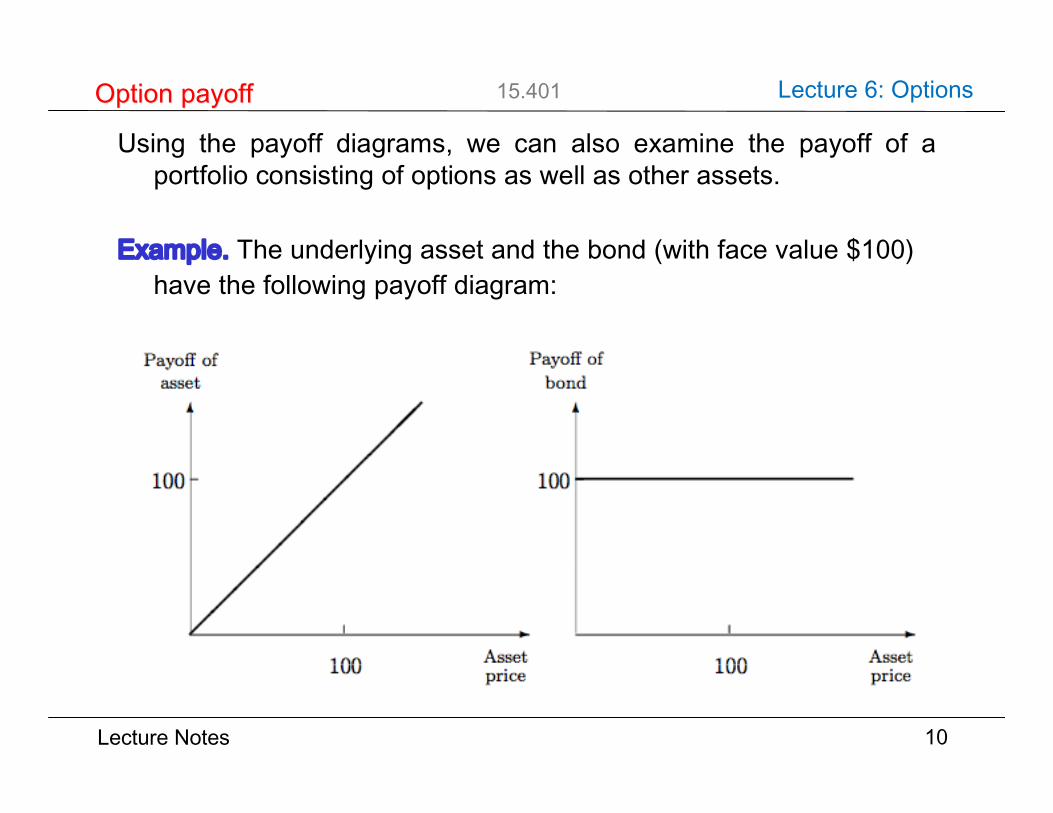
Using the payoff diagrams, we can also examine the payoff of aportfolio consisting of options as well as other assets.

Example. The underlying asset and the bond (with face value $100)have the following payoff diagram:

10


-

6

Assetprice

Payo®ofa straddle

100

100

@@

@@

@@

@@

¡¡

¡¡

¡¡

¡¡

Lecture Notes


Stock + put

11

Option strategiesOption strategies

-

6

Asset

PutAssetprice

Payo®ofasset & put

100

100

¡¡

¡¡¡

¡¡

@@

@@

@@

-

6

Net payo®

Assetprice

Payo®ofasset + put

100

100 ¡¡ ¡

Lecture Notes


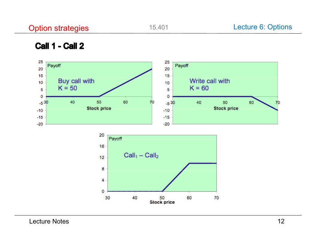
Call 1 - Call 2

12


-

6

Assetprice

Payo®ofa call

100

100

¡¡

¡¡

¡¡

-

6

Assetprice

Payo®ofa put

100

100

@@

@@

@@

Lecture Notes


-

6

Assetprice

Payo®ofa straddle

100

100

@@

@@

@@

@@

¡¡

¡¡

¡¡¡¡

13


Call + Put

Lecture Notes


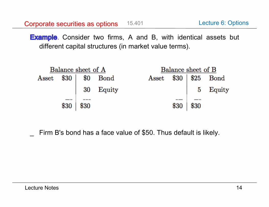
Example. Consider two firms, A and B, with identical assets butdifferent capital structures (in market value terms).

_ Firm B's bond has a face value of $50. Thus default is likely.

14

Corporate securities as optionsCorporate securities as options

Balance sheet of A Balance sheet of BAsset $30 $0 Bond Asset $30 $25 Bond

30 Equity 5 Equity

$30 $30 $30 $30

Lecture Notes


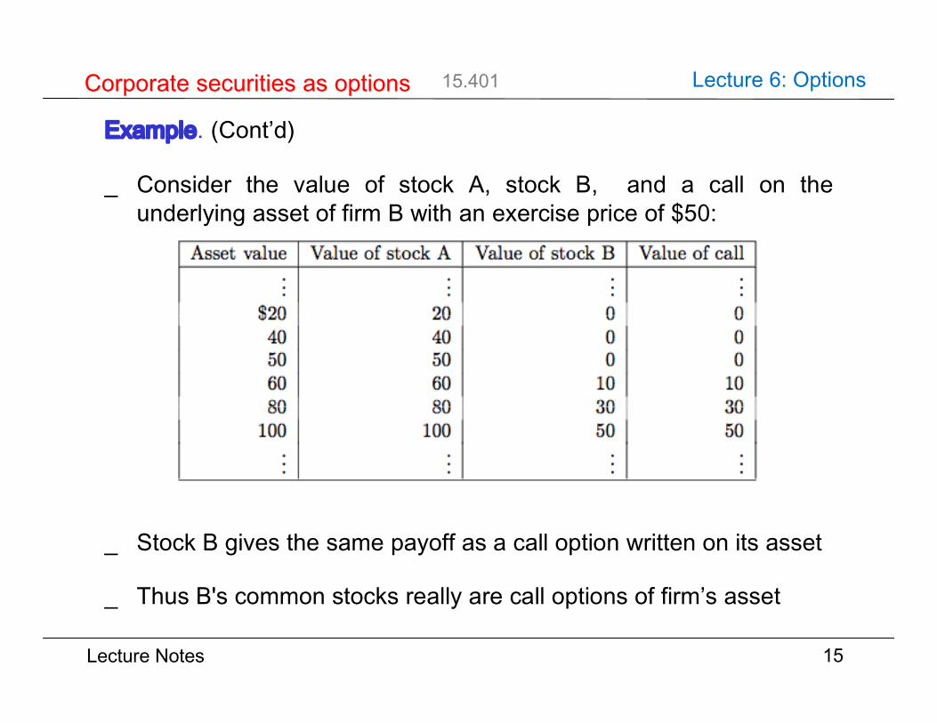
Example. (Cont’d)

_ Consider the value of stock A, stock B, and a call on theunderlying asset of firm B with an exercise price of $50:

_ Stock B gives the same payoff as a call option written on its asset

_ Thus B's common stocks really are call options of firm’s asset

15


Lecture Notes


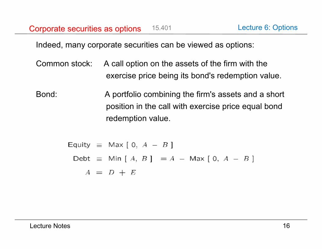
Indeed, many corporate securities can be viewed as options:

Common stock: A call option on the assets of the firm with the exercise price being its bond's redemption value.

Bond: A portfolio combining the firm's assets and a short position in the call with exercise price equal bond redemption value.

16


Lecture Notes


Warrant: Call options on the stock issued by the firm.

Convertible bond: A portfolio combining straight bonds and a call option on the firm's stock with the exercise price related to the conversion ratio.

Callable bond: A portfolio combining straight bonds and a call written on the bonds.

17


Lecture Notes


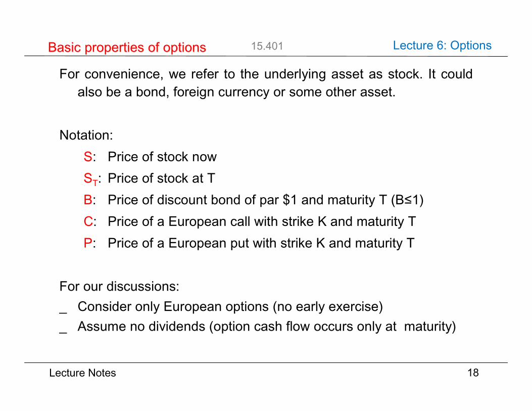
For convenience, we refer to the underlying asset as stock. It couldalso be a bond, foreign currency or some other asset.

Notation:S: Price of stock nowST: Price of stock at TB: Price of discount bond of par $1 and maturity T (B≤1)C: Price of a European call with strike K and maturity TP: Price of a European put with strike K and maturity T

For our discussions:_ Consider only European options (no early exercise)_ Assume no dividends (option cash flow occurs only at maturity)

18

Basic properties of optionsBasic properties of options

Lecture Notes


First consider European options on a non-dividend paying stock.

1. C ¸ 0

2. C · S

The payoff of stock dominates that of call:

19

Price boundsPrice bounds

-

6

ST

Payo®

K

K

bbbbbbbbbbbbbbbbbbbb

¡¡¡¡

¡¡

¡¡¡

stock

call

Lecture Notes


3. C ¸ S - K BStrategy (a): Buy a callStrategy (b): Buy a share of stock by borrowing KB

The payoff of strategy (a) dominates that of strategy (b):

Since C ¸ 0, we have

20


-

6

ST

Payo®

K

¡¡

¡¡

¡¡ ¡

bbbbbbbbbbbbbbbbbbbb

strategy (b)

call

C ¸ max[S ¡ KB, 0]

Lecture Notes


4. Combining the above, we have

21


max[S ¡ KB, 0] · C · S

-

6

Stock price

Optionprice

KB

¡¡¡

¡¡

¡¡¡

¡¡

¡¡

¡¡ ¡

¡¡

¡¡

¡¡¡

¡¡

¡¡¡

¡¡ ¡

upperbound

lowerboundoption

price

Lecture Notes


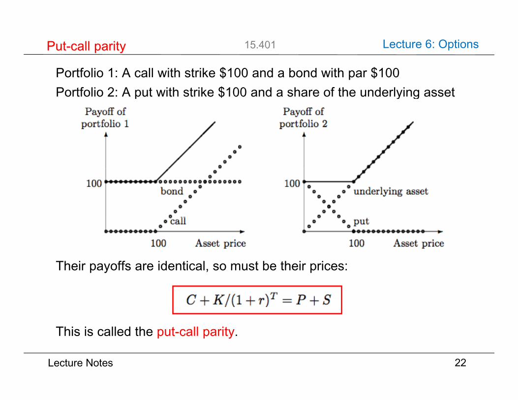
Portfolio 1: A call with strike $100 and a bond with par $100Portfolio 2: A put with strike $100 and a share of the underlying asset

Their payoffs are identical, so must be their prices:

This is called the put-call parity.

22

Put-call parityPut-call parity

-

6

Asset price

Payo®ofportfolio 1

100

100 ¡¡

¡¡

¡¡

aaaaaaaaaaaaaaaaaaaaaaaaaaaa

aaaaaaaaaaaaaaaaaaaaaaaaaaaa

bond

call -

6

Asset price

Payo®ofportfolio 2

100

100 ¡¡¡

¡¡¡

aaaaaaaaaaa

aaaaaaaaaaaaaaaaaaaaaaaaaaaaaaaaaaaaa

underlying asset

put

C +K/(1 + r)T = P + S

Lecture Notes


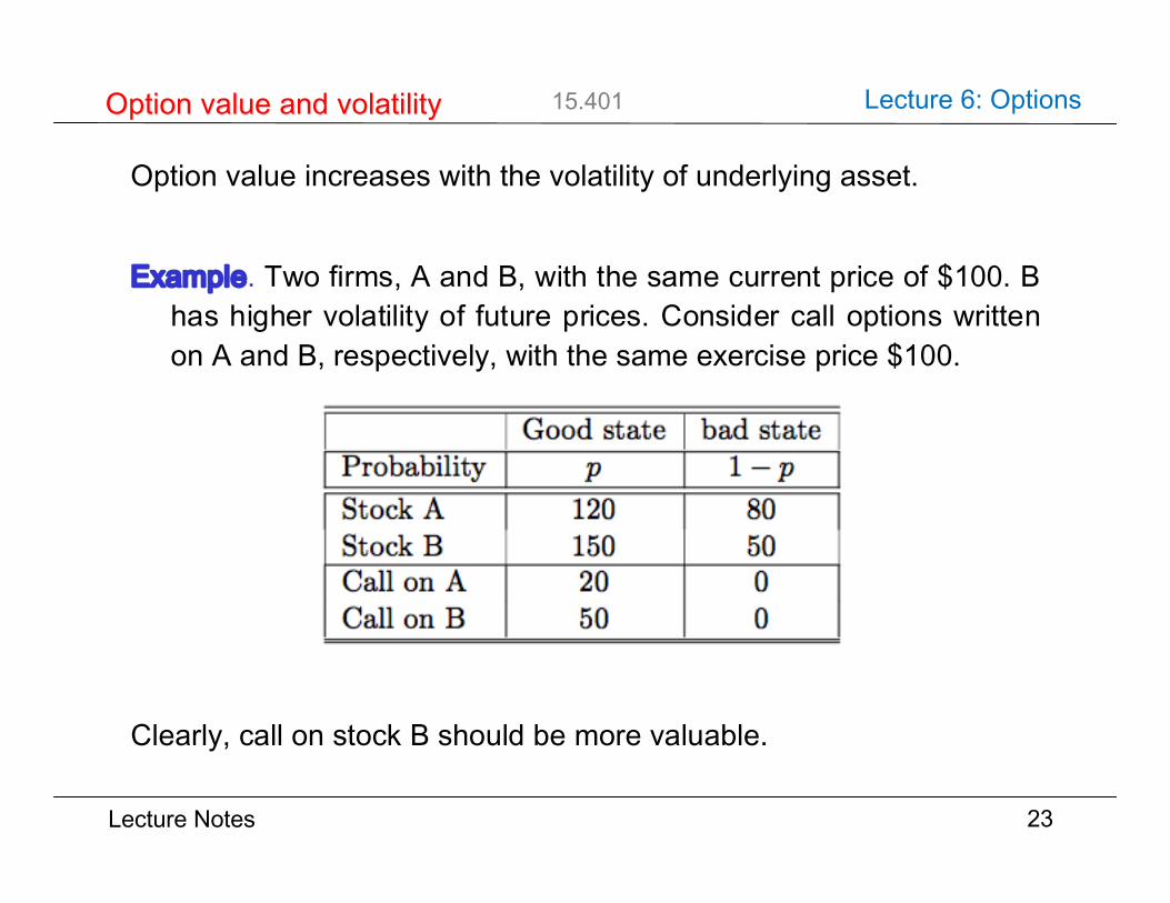
Option value increases with the volatility of underlying asset.

Example. Two firms, A and B, with the same current price of $100. Bhas higher volatility of future prices. Consider call options writtenon A and B, respectively, with the same exercise price $100.

Clearly, call on stock B should be more valuable.

23

Option value and volatilityOption value and volatility

Good state bad stateProbability p 1 ¡ pStock A 120 80Stock B 150 50Call on A 20 0Call on B 50 0

Lecture Notes


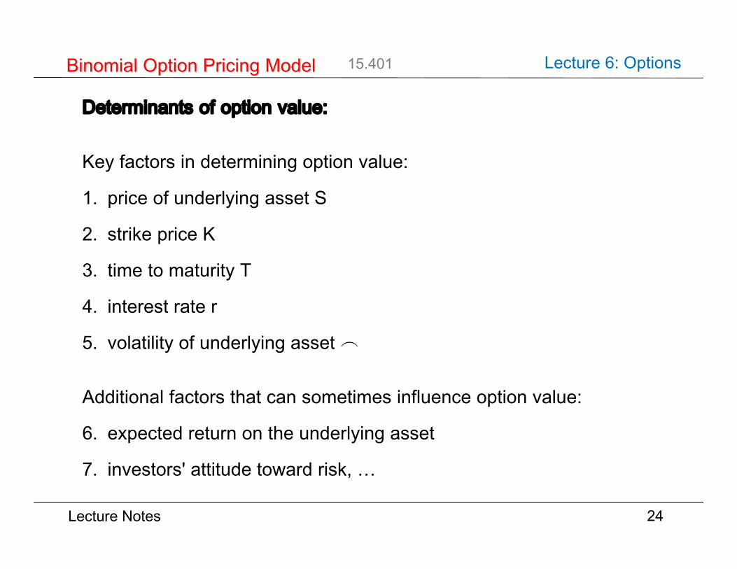
Determinants of option value:

Key factors in determining option value:

1. price of underlying asset S

2. strike price K

3. time to maturity T

4. interest rate r

5. volatility of underlying asset _

Additional factors that can sometimes influence option value:

6. expected return on the underlying asset

7. investors' attitude toward risk, …

24

Binomial Option Pricing ModelBinomial Option Pricing Model

Lecture Notes


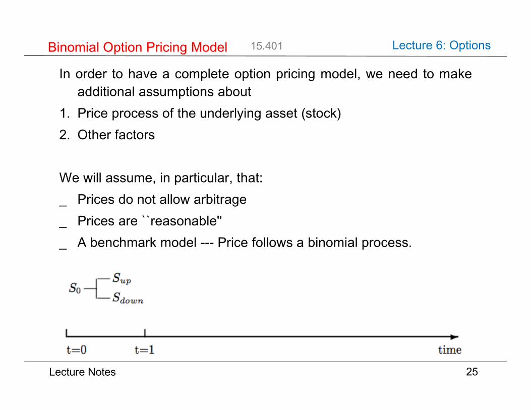
In order to have a complete option pricing model, we need to makeadditional assumptions about

1. Price process of the underlying asset (stock)2. Other factors

We will assume, in particular, that:_ Prices do not allow arbitrage_ Prices are ``reasonable''_ A benchmark model --- Price follows a binomial process.

25


-t=0 t=1 time

S0Sup

Sdown

Lecture Notes


Example. Valuation of a European call on a stock._ Current stock price is $50_ There is one period to go_ Stock price will either go up to $75 or go down to $25_ There are no cash dividends_ The strike price is $50_ One period borrowing and lending rate is 10%

The stock and bond present two investment opportunities:

The option's payoff at expiration is:

What is C0, the value of the option today?

26


5075

251

1.1

1.1C0

25

0

Lecture Notes


Form a portfolio of stock and bond that replicates the call’s payoff: a shares of the stock b dollars in the riskless bond

such that

Unique solution:That is

– buy half a share of stock and sell $11.36 worth of bond– payoff of this portfolio is identical to that of the call– present value of the call must equal the current cost of this

``replicating portfolio'' which is

Number of shares needed to replicate one call option is called theoption’s hedge ratio or delta.

In the above problem, the option’s delta is a = 1/2.27


75a+ 1.1b = 25

25a+ 1.1b = 0

a = 0.5 and b = ¡ 11.36(50)(0.5) ¡ 11.36 = 13.64

Lecture Notes


More than one period:

Call price process:

_ terminal value of the call is known, and_ Cu and Cd denote the option value next period when the stock

price goes up and goes down, respectively_ Compute the current value by working backwards: first Cu and Cd

and then C28


S=50

75112.5

37.5

2537.5

12.5

C

CuCuu = 62.5

Cud = 0

CdCdu = 0

Cdd = 0

Lecture Notes


Step 1. Start with Period 1:1. Suppose the stock price goes up to $75 in period 1:_ Construct the replicating portfolio at node ( t =1, up):

_ Unique solution: a = 0.833, b = - 28.4_ The cost of this portfolio: (0.833)(75) ‒ 28.4 = 34.075_ The exercise value of the option: 75 ‒ 50 = 25 ≤ 34.075_ Thus, Cu = 34.075.

2. Suppose the stock price goes down to $25 in period 1. Repeat theabove for node (t =1, down):

_ The replicating portfolio: a = 0, b = 0_ The call value at the lower node next period is Cd = 0.

29

Two-period Binomial ModelTwo-period Binomial Model

112.5a+ 1.1b = 62.5

37.5a+ 1.1b = 0

Lecture Notes


Step 2. Now go back one period, to Period 0:_ The option's value next period is either 34.075 or 0:

_ If we can construct a portfolio of the stock and bond to replicatethe value of the option next period, then the cost of this replicatingportfolio must equal the option's present value.

_ Find a and b so that

_ Unique solution: a = 0.6815, b = -15.48_ The cost of this portfolio: (0.6815)(50) ‒ 15.48 = 18.59_ The present value of the option must be C0 = 18.59_ It is greater than the exercise value 0 (thus no early exercise)

30


C0Cu = 34.075

Cd = 075a+ 1.1b = 34.075

25a+ 1.1b = 0

Lecture Notes


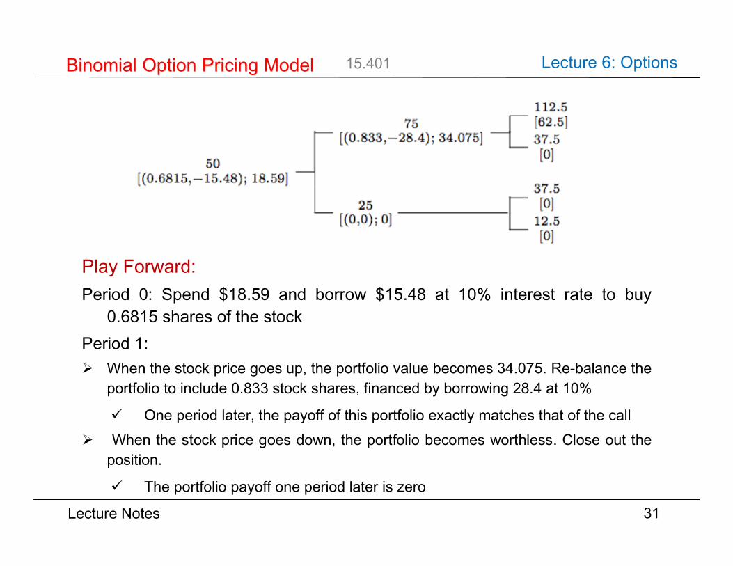
Play Forward:Period 0: Spend $18.59 and borrow $15.48 at 10% interest rate to buy

0.6815 shares of the stockPeriod 1: When the stock price goes up, the portfolio value becomes 34.075. Re-balance the

portfolio to include 0.833 stock shares, financed by borrowing 28.4 at 10%

One period later, the payoff of this portfolio exactly matches that of the call When the stock price goes down, the portfolio becomes worthless. Close out the

position.

The portfolio payoff one period later is zero

31


50[(0:6815;¡ 15:48); 18:59]

75[(0:833;¡ 28:4); 34:075]

112:5[62:5]37:5[0]

25[(0;0); 0]

37:5[0]12:5[0]

Lecture Notes


Thus

_ No early exercise.

_ Replicating strategy gives payoffs identical to those of the call.

_ Initial cost of the replicating strategy must equal the call price.

32


Lecture Notes


What we have used to calculate option's value:_ current stock price_ magnitude of possible future changes of stock price -- volatility_ interest rate_ strike price_ time to maturity

What we have not used:_ probabilities of upward and downward movements_ investor's attitude towards risk

Questions on the Binomial ModelQuestions on the Binomial Model_ What is the length of a period?_ Price can take more than two possible values._ Trading takes place continuously.

33


Lecture Notes


If we let the period-length get smaller and smaller, we obtain theBlack-Scholes option pricing formula:

where

_ x is defined by

_ T is in units of a year

_ R = 1+r, where r is the annual riskless interest rate

_ σ is the volatility of annual returns on the underlying asset

_ N (.) is the cumulative normal density function

34

Black-Black-Scholes formularScholes formular

C(S,K, T ) = SN

µx

¶¡ KR¡ TN

µx ¡

pT

¶

x =

ln

µS/KR¡ T

¶

pT

+1

2

pT

Lecture Notes


An interpretation of the Black-Scholes formula:

_ The call is equivalent to a levered long position in the stock.

_ S N(x) is the amount invested in the stock

_ is the dollar amount borrowed

_ The option delta is

35

Black-Black-Scholes Scholes formulaformula

SN(x)N(x) = CS

Lecture Notes


Example. Consider a European call option on a stock with thefollowing data:

_ S = 50, K = 50, T = 30 days_ The volatility σ is 30% per year_ The current annual interest rate is 5.895%

Then

36

Black-Black-Scholes Scholes formulaformula

x =

ln

µ50/50(1.05895)¡ 30

365

¶

(0.3)q

30365

+1

2(0.3)

q30365 = 0.0977

C = 50N(0.0977) ¡ 50(1.05895)¡ 30365N

≥0.0977¡ 0.3

q30365

´

= 50(0.53890) ¡ 50(0.99530)(0.50468)

= 1.83

Lecture Notes


_ Introduction to options

_ Option payoffs

_ Corporate securities as options

_ Use of options

_ Basic properties of options

_ Binomial Option Pricing Model

_ Black-Scholes option pricing formula

37

Key conceptsKey concepts

15.401 Finance Theory I - MITweb.mit.edu/astomper/www/univie/pof/Chapter 6.pdf · _Brealey, Myers...

Documents

Transcript of 15.401 Finance Theory I - MITweb.mit.edu/astomper/www/univie/pof/Chapter 6.pdf · _Brealey, Myers...