14th CIRIAF National Congress PDF final

Printed Edition of the Special Issue Published in Sustainability

14th CIRIAF National Congress – Energy, Environment andSustainable Development

Edited by

Francesco Asdrubali and Franco Cotana

www.mdpi.com/journal/sustainability

Francesco Asdrubali and Franco Cotana (Eds.)

14th CIRIAF National Congress –Energy, Environment and Sustainable Development

This book is a reprint of the Special Issue that appeared in the online, open access journal,Sustainability (ISSN 2071-1050) in 2014 (available at: http://www.mdpi.com/journal/sustainability/special_issues/ciriaf).

Guest EditorsFrancesco Asdrubali and Franco CotanaDepartment of EngineeringUniversity of PerugiaVia G. Duranti 67, 06125 PerugiaItaly

Editorial OfficeMDPI AGKlybeckstrasse 64Basel, Switzerland

PublisherShu-Kun Lin

Managing EditorLe Zhang

1. Edition 2015

MDPI • Basel • Beijing • Wuhan • Barcelona

ISBN 978-3-03842-097-2 (Hbk)ISBN 978-3-03842-098-9 (PDF)

Articles in this volume are Open Access and distributed under the Creative Commons Attribution license (CC BY), which allows users to download, copy and build upon published articles even for commercial purposes, as long as the author and publisher are properly credited, which ensures maximum dissemination and a wider impact of our publications. The book taken as a whole is © 2015 MDPI, Basel, Switzerland, distributed under the terms and conditions of the Creative Commons by Attribution (CC BY-NC-ND) license (http://creativecommons.org/licenses/by-nc-nd/4.0/).

Angelamaria Massimo, Marco Dell'Isola, Andrea Frattolillo and Giorgio Ficco

2014 ï

Cinzia Buratti, Elisa Moretti, Elisa Belloni and Fabrizio Agosti

2014 ï

Francesco Leccese, Giacomo Salvadori, Matteo Casini and Marco Bertozzi

2014 ï

Federico Rossi, Andrea Nicolini, Massimo Palombo, Beatrice Castellani, Elena Morini and Mirko Filipponi

2014 ï

Biancamaria Torquati, Sonia Venanzi, Adriano Ciani, Francesco Diotallevi and Vincenzo Tamburi

2014 ï

Beatrice Castellani, Elena Morini, Mirko Filipponi, Andrea Nicolini, Massimo Palombo, Franco Cotana and Federico Rossi

2014 ï

Andrea Presciutti, Francesco Asdrubali, Assunta Marrocchi, Alessandra Broggi,Giuliano Pizzoli and Alessio Damiani

2014 ï

Dario Ambrosini, Giorgio Galli, Biagio Mancini, Iole Nardi and Stefano Sfarra

2014 ï

Francesco Bianchi, Anna Laura Pisello, Giorgio Baldinelli and Francesco Asdrubali

2014 ï

Andrea de Lieto Vollaro, Giuseppe De Simone, Roberto Romagnoli, Andrea Vallati and Simone BotilloNumerical Study of

2014 ï

Francesco Fassio, Aldo Fanchiotti and Roberto de Lieto Vollaro

2014 ï

Fabrizio Agosti: .Dario Ambrosini:

.Francesco Asdrubali: .Giorgio Baldinelli: .Elisa Belloni:

.Marco Bertozzi:

.Francesco Bianchi: .Simone Botillo:

.Alessandra Broggi:

.Cinzia Buratti:

.Matteo Casini:

.Beatrice Castellani:

.Adriano Ciani:

.Franco Cotana:

.Alessio Damiani: .Giorgio Galli:

.Andrea de Lieto Vollaro:

.Roberto de Lieto Vollaro:

.

Giuseppe De Simone:.

Marco Dell'Isola:.

Francesco Diotallevi:.

Aldo Fanchiotti:.

Francesco Fassio:.

Giorgio Ficco:.

Mirko Filipponi:.

Andrea Frattolillo:.

Francesco Leccese:

.Biagio Mancini:

.Assunta Marrocchi:

.Angelamaria Massimo:

.Elisa Moretti:

.Elena Morini:

.Iole Nardi:

.Andrea Nicolini:

.Massimo Palombo:

.Anna Laura Pisello:

.Giuliano Pizzoli: .

Andrea Presciutti: .Roberto Romagnoli:

.Federico Rossi:

.Giacomo Salvadori:

.Stefano Sfarra:

.Vincenzo Tamburi:

.Biancamaria Torquati:

.Andrea Vallati:

.Sonia Venanzi:

.Andrea de Lieto Vollaro:

.

VIII

About the Guest Editors Franco Cotana was born in Marsciano, Perugia in 1957. He graduated with a degree in electrical engineering in 1983 from the University of Rome “La Sapienza”. He is now a Full Professor in “Industrial Applied Physics” at the University of Perugia. Since 2014, Prof. Cotana has been a Member of the Board of Administration of the University of Perugia. From 2013 to 2015, Franco Cotana was the Director of CIRIAF (the Inter-University Research Center for Pollution and Environment – Mauro Felli), which is based at the University of Perugia. From 2003 to 2013, Prof. Cotana was also the Director of CRB (National Biomass Research Center), a research center of the University of Perugia that is sponsored by the Italian Ministry of Environment, Sea and Land Protection. He is the President and Coordinator of the PhD program in “Energy Engineering” at the University of Perugia. Franco Cotana is a Teacher of Applied Physics, Course on Mechanical Engineering at the University of Perugia. He is also a Teacher of air conditioning systems and renewable energy, Course on Architectural Engineering at the University of Perugia. Prof. Cotana is the author of more than 280 scientific papers and has 18 patents in the fields of energetics, applied acoustics, heat transfer, applied thermodynamics, and lighting design. He is the Coordinator of many national and international research projects. Prof. Cotana is also a Member of the New York Academy of Sciences. He is also a Representative of the Italian Government in Brussels for the EIBI SET PLAN. Finally, Prof. Cotana is a Member of the Coordination Board of the AIA-IPPC Commission at the Italian Ministry for the Environment, Sea and Land Protection. Francesco Asdrubali is an Associate Professor of environmental applied physics at the University of Perugia. Born in Perugia in 1967, Prof. Asdrubali graduated with a degree in civil engineering in 1990 and then obtained a PhD in the thermophysical properties of materials in 1995. From 2004 to 2013, Francesco Asdrubali was the Director of CIRIAF, an Inter-University Research Center in the field of environmental science and pollution, which is based at the University of Perugia. Prof. Asdrubali is an instructor of: energy systems and the environment, renewable energies, environmental acoustics, and applied thermodynamics and heat transfer. He is a Member of the Faculty of Engineering at the University of Perugia. He is also the Coordinator of the Socrates Intensive Programs, the Coordinator of various Erasmus agreements, and the Erasmus Delegate of the Department of Engineering since 2014. Prof. Asdrubali is also the coordinator of various international research programs: the British-Italian Joint Research Program with the University of Bradford (UK), the Vigoni Program with the Technical University of Berlin (Germany), and various EU- funded Projects (LIFE, Intelligent Energy Europe, VII FP). His areas of scientific research include: renewable and alternative energies, heat transfer, energy and buildings, life cycle assessment, acoustical properties of materials, environmental noise, natural and artificial lighting, and sustainable mobility. Francesco Asdrubali is the author of more than 200 scientific papers in the above mentioned areas. In 2014, he obtained habilitation as a full professor at the national scientific professorship competition.

1

Development of a Geographical Information System (GIS) for the Integration of Solar Energy in the Energy Planning of a Wide Area

Angelamaria Massimo, Marco Dell’Isola, Andrea Frattolillo and Giorgio Ficco

Abstract: Energy planning has become one of the most powerful tools for urban planning even if several constraints, (i.e., aesthetic, archaeological, landscape) and technological (low diffusion of Renewable Energy Sources, RES) reduce its spreading. An efficient and sustainable urban planning process should be based on detailed energy issues, such as: (i) the effective energetic characteristics and needs of the area like urban density and energy consumption, (ii) the integration of different RES and (iii) the diffusion of high efficiency technologies for energy production like cogeneration and district heating. The above-mentioned energetic issues and constraints must be constantly updated, in order to evaluate the consequences on environment and landscape due to new distributed generation technologies. Moreover, energy strategies and policies must be adapted to the actual evolution of the area. In this paper the authors present a Geographical Information Database System (GIS DB) based on: (i) the availability of land use (Land Capability Classification, LCC) to evaluate the productive potential; (ii) the estimation of residential energy consumptions (e.g., electricity), (iii) the integration of RES. The GIS DB model has been experimented in a wide area of Central Italy, considering exclusively the solar energy source for energy generation.

Reprinted from Sustainability. Cite as: Massimo, A.; Dell’Isola, M.; Frattolillo, A.; Ficco, G. Development of a Geographical Information System (GIS) for the Integration of Solar Energy in the Energy Planning of a Wide Area. Sustainability 2014, 6, 5730–5744.

1. Introduction

The rapid increase in world population, together with the progressive urbanization has led more than 50% of the world population to live in urban areas. Moreover, according to United Nations (UN) more than 70% of the total population is going to live in cities by 2050 [1]. Therefore, management and environmental issues of the cities are on the rise and environmental regulations become more strict and numerous [2–4]. Nevertheless, for an effective management of the cities, not only environmental issues but also human needs must be considered, providing adequate infrastructures for the increasing number of citizens despite the limited availability of resources, especially the energetic ones. Furthermore, at the current rate of urbanization and considering the actual social and environmental needs, urban energy networks (i.e., gas, water, electricity, and heat) are to be necessarily extended and, possibly, integrated with RES. As regards buildings, the new constructions are requested to be designed with energy efficiency criteria in mind, whereas the existing ones should be adequately renovated to get a more effective energy performance. As a consequence, actual cities are going to be reorganized and modern tools must be appropriately designed for urban management and planning.

2

To achieve a real sustainable development, European Union (EU) needs efficient tools to facilitate the urban planning and management process. The last 50 years deeply changed urban planning approach. In fact, in the 1960s a systemic approach was in force. Cities were considered as a sum of subsystems in which quantitative top-down models were used capable of providing reliable predictions of public decisions. Later, firstly in the United States (US) and then in EU, the “planning business type” model had spread and the strategic planning tools typical of large enterprises were used also for cities management needs. At the end of the 1990s, finally, a strategic “reticulated structure” planning has spread, with multiple levels, able to allow expertise in urban and environmental planning at administrative bodies level (i.e., regions, provinces and municipalities). For reasons of clarity, the Province is an Italian Administrative body which groups together more neighbouring municipalities. As an example, the Province of Frosinone, investigated by the authors in the present paper, presents a territorial extension of 3.243 km2 and it is made up of 91 municipalities.

However, all the above traditional approaches were addressed exclusively to rule the expansion of existing urban areas without taking into account the principles of a real sustainable development (e.g., economic, social and environmental sustainability). Only in recent years, urban planning tools integrated with energy issues were adopted [5–7], defining primary targets in terms of reduction of energy consumption and of the introduction of Renewable Energy Sources (RES) [8], especially in residential sector (that is responsible of about 40% of energy consumptions and of about 36% of CO2 emissions [9]). As a consequence, self-sufficient buildings with low energy consumption (the so-called “nearly zero energy buildings”) [9] are more and more spreading.

The “interference” between the buildings and the urban context is not only due to architectural and landscape aspects, but also (and especially) to energetic ones, like: (i) solar gains; (ii) soil or groundwater cooling/heating (i.e., low enthalpy geothermal energy); (iii) the variable intensity and direction of the wind in the so called “street canyons” (i.e., wind energy); (iv) the environmental impact of biomasses [10]. On the other hand, the need to maximize efficiency of cities should increase the knowledge of any excess/deficit of energy and promote “smart grid” in urban contexts [11,12].

In the literature some solar energy availability models in urban districts are available [13–15]. Further models provide issues related to orientation and shape of solar energy panels [16,17] in order to maximize the production of solar energy [18]. Cellura et al. [19] evaluated the relationship between the surface of the rooftops and the height of the buildings, providing a first tool to analyze the influence of the density of the built environment on the availability of solar energy. Furthermore, in [20,21], the evolution of energy supply in specific areas is evaluated through the use of GIS, to predict the energy demand and to estimate the optimal location of new RES in respect to the existing power grids. However, the aspects related to a strict integration between RES and high-efficiency power generation systems, such as cogeneration and district heating, have been not fully investigated in high-density urban contexts.

3

In the so-called “Smart City”, the involvement of the population in the design of urban interventions and the use of new information technologies, should improve the life quality. However, being “smart” means that city must have a “brain”. This means that an effective information system must be available to integrate and manage huge amount of data on mobility, air and environmental conditions, waste, energy efficiency and utilities, etc. All the above-mentioned data present very fast spatial dynamics and the use of proximity, inclusion, adjacency criteria, and so on, are strongly encouraged. This is the reason why the “Geographic” characteristic of any Information System adopted plays a crucial role.

Several GIS applications in Smart Cities are now available. In [22], the implementation of a GIS allows to: (i) locate sport facilities in Rome and to analyze the demand and supply of sports; (ii) to access and update many aspects of urban life in Modena (i.e., building heritage, energy consumption, city companies, and maintenance of green areas); (iii) to evaluate energy consumptions and to test some bio-architecture and green building strategies on a medium-size urban area; (iv) to plan the exploitation of lands with poor agricultural potential (or unsuitable for residential purposes) for biofuel crops production [23].

In this paper the authors describe the results of the application of a Geographical Information Database System (GIS DB) energy-planning model, taking into account some crucial energetic parameters for urban sustainability. The GIS DB model proposed has been experimented in the Province of Frosinone, which is a wide area in the Lazio Region in Central Italy. The investigated area is particularly interesting for the morphology, for the poor energetic performance of the existing buildings and for the climatic, environmental, and landscape peculiarities of the territory.

2. Methodology

According to Directive 2009/28/CE [6] on the promotion of RES, all EU members States are committed to adopt a national action plan based on the principles of sustainability. This means to analyze the status of each territory and to predict future scenarios in terms of energetic demand, availability and production of RES and greenhouse gas emissions. Therefore, knowledge of available energy sources together with the localization of energy production facilities and of transmission and distribution infrastructures are crucial tasks for any urban planning at local level. These information, on extended territories, such as Provinces in Italy, often need a “multicriteria analysis” of different variables such as: (i) geographical (latitude, longitude, exposure, altitude above sea level); (ii) physical-morphological characteristics (slope, hydraulic jumps, presence of hills and obstacles) of the territory; (iii) the land use (e.g., the presence of forests and crops); (iv) the distance of RES from cities or from the connection infrastructure to the national grid; etc.

In this paper, the authors present a model, which uses the functions and raster data-grid as a tool for the analysis of the many quantitative assessments necessary in the planning phase. The model has been developed and experimented in the Province of Frosinone, which is an area particularly interesting for its morphology, the poor energetic performance of buildings, and climatic peculiarities of the territory. The model manages the data related only to the “solar energy”, and it is aimed to analyze, exhaustively, the different energy production scenarios in the Province of Frosinone. The area is surrounded by mountain ranges (the Central Apennines to the north and the

4

pre-Apennines of Lazio to the south) separated by a vast territory (the Valle Latina) in which the Sacco and Liri rivers flow. Since topography influences the area from a climatic point of view (without predominant winds and periods of high rains and humidity), industrial and urban settlements cause serious environmental problems in terms of pollution of soil, rivers, and air. The Province of Frosinone, in fact, is crossed from NW to SE by the A1 highway from Rome to Naples, which is characterized by large volumes of vehicular traffic. Along the A1, numerous industrial settlements are present (i.e., the industrial districts of Frosinone-Anagni in the north and Cassino in the south) with several large, medium, and small factories. Moreover, the presence of different industry typologies (e.g., food, chemical-pharmaceutical, automotive, mills) causes different impacts on the environment and present very different energy needs.

The analysis of production from solar energy cannot be separated from a detailed knowledge of the real solar energy availability in the area. Therefore, the use of updated maps and spatially distributed databases to evaluate the potential solar energy distribution should be strongly encouraged. To correctly determine the spatial variations of solar radiation into morphologically complex areas, such as the Province of Frosinone, it is necessary to integrate analytical models of solar radiation on a GIS basis with the information provided in high-resolution data sets, such as DEM (Digital Elevation Model). These models [23–28] are based on empirical physical equations, providing accurate estimates of solar radiation as well as the geographical location and the morphological characteristics of the area. In the proposed model, data are managed using the Solar Analyst model developed by ESRI ArcGIS 10® and modified according to [29]. The GIS DB model for the Province of Frosinone was further implemented with raster grid for the analysis of: (i) the real land use, (ii) the possibility of exploitation of photovoltaic technology in urban areas, (iii) the electricity consumption and their geographical distribution, and (iv) the power generation facilities installed and their energy production estimates.

2.1. Land Use

In order to get a complete representation of the use of the soil, thematic maps developed by the CORINE-Land Cover Project [30] were analyzed, classifying the Province of Frosinone into artificial surfaces (territories morphologically altered by human presence, such as the urban centers), agricultural, forest, and water bodies (Figure 1).

In particular, agricultural areas have been classified according to the actual land use as reported in Table 1.

Since forest and semi natural areas are subject to environmental protection, solar energy exploitation is really obtainable only in agricultural lands and in urban contexts. As regards agricultural lands, it has be pointed out that the Italian Decree n. 28 of 2011 [31] sought to limit the spread of solar energy plants on land intended for other uses by providing that, for the same owner: (i) nominal power of each plant do not exceed 1 MW; (ii) different solar plants are to be placed at a minimum distance of 2 km; (iii) solar plant area not exceeding 10% of the land of the owner. The Decree Law n. 1 of 2012 [32] reinforced these constraints, prohibiting access to government incentives to any plant with solar panels located on land in agricultural areas.

5

Figure 1. Land use of the Frosinone Province.

Table 1. Agricultural surface classification.

Arable land Non-irrigated arable land

Permanently irrigated land

Permanent crops

Vineyards Fruit trees and berry plantations

Olive groves Other permanent crops

Pastures Pastures

Heterogeneous agricultural

areas

Annual crops associated with permanent crops Complex cultivation patterns

Land principally occupied by agriculture, with significant areas of natural vegetation

Agro-forestry areas

With the end of government incentives in Italy [33], all the above constraints are now automatically forfeited and landowners have full autonomy in sizing photovoltaic systems on their land. Moreover, all the agricultural lands of the Province of Frosinone sum about 1901 km2, corresponding to a potential annual net energy production of 30.0 × 104 GWh, considering an average radiation annual of 1600 kWh/m2 and an average efficiency of 14% for solar panels. Although the lack in Italy of a specific regulation, the authors exclude from this estimation the permanent crops (the so-called “Prime farmland” [34]) in order to avoid the loss of soils fertility. Therefore, the available area exploitable for solar energy production should be limited to pastures and heterogeneous agricultural lands (Table 1) and the total available area reduces to about 778 km2 (corresponding to 12.4 × 104 GWh of annual net energy production potentially obtainable). The

6

overlap of solar radiation and potentially exploitable lands for the Province of Frosinone, is shown in Figure 2.

Figure 2. Overlapping of solar radiation in the areas exploitable for solar energy production.

From Figure 2, it can be noticed that the actually exploitable lands are located in the valley areas of the Province, and often close to cities. Therefore, the installation of solar energy plants will allow the requalification of such areas and, moreover, solar energy production facilities will be close to urban areas where the higher energy demand and the lower possibility of RES integration are present.

2.2. The Urban Context

The energetic producibility of RES plants, and the convenience to integrate solar energy panels in urban contexts with high building density, must be evaluated taking into account: (i) the typology, slope, aspect, and useful surface of the roofs [13,17,35]; (ii) the theoretical energy production of solar panels; (iii) the economic analysis (i.e., the payback time) according to the real energetic needs of users (e.g., single apartments, condominiums, and blocks) [19]. Firstly, it is necessary to analyze the roofs typology based on morphology and building materials. In this paper two main classifications are considered: tile roofs (pitched) and flat roof. The developed algorithm firstly identifies the roof typology from the color (i.e., from average value of pixels) of the roofs. Subsequently, the photogrammetric image is crossed with the digital orthophotography. As an example, Figure 3 shows the displaying of digital orthophotography and the identification of the geometry of roofs in residential areas.

7

Figure 3. Roofs classification of residential units.

The data related to the slope of pitched roof are not directly obtainable from photogrammetric since the heights of gutters and hipped roofs are not evaluable. Consequently, theoretical data based on average slopes related to precipitations have been used. In particular, for the present case of study, an average slope of 30% has been considered.

When the classification of the roofs is completed, it is important to evaluate the useful area of solar radiation incidence. The presence of obstacles (e.g., windows, chimneys, and stairwells) causes a reduction of useful spaces for the installation of solar panels. Since it is impossible to take into account the presence of obstructions on the roofs, it was assumed a useful area of about 80% for flat roofs, and 25% for pitched roofs. All the structural information obtained have been integrated in a 3D building model (Digital Elevation Model-DEM) and detailed in a specific database of the investigated buildings. Then, building database was used to estimate both the global solar radiation and the theoretical energy production of buildings through the specific tool of the Solar Radiation ArcGIS [36]. A typical result of this analysis is shown in Figure 4.

Figure 4. Theoretical energy production of individual residential units (kWh/m2).

2.3. Analysis of Local Consumption

An adequate energy planning cannot neglect its energetic balance through the estimation of energy consumption distribution in the territory. In Figure 5, the 2011 Energy Balance of the Province of Frosinone is reported for different sectors [37].

8

Figure 5. Energy consumption in the Province of Frosinone (2011) for different sectors.

As regards energy consumptions in the investigated area, the authors considered only electricity ones, for which it is evident an unbalance between industrial (59%) and residential, commercial and public (34%) and sectors. Different demographic and socioeconomic data [38] have been also considered, such as, the total floor area of the buildings, the population density, the number of residential buildings, etc. In fact, the domestic energy consumption and the population density are useful indicators to estimate human impact on the environment. However, this latter is strongly influenced by the geophysical characteristics of the area, which may include low-density areas (i.e., high mountains, water surfaces, etc.), as well as urban or rural settlements. As an example, the assessment of domestic consumption is difficult because of numerous aspects: geographical location, season of the year, day of the week, energy habits of the households, characteristics of housing, household electrical appliances and so on.

Therefore, adopting for the investigated area the data of electric energy consumption available at national level [39], the following relationships emerge: (a) a direct proportionality between energy consumptions and the total floor area of the buildings in the domestic sector; (b) a direct proportionality of consumption with the Gross Domestic Product and the territorial extension for the tertiary sector (hotels, banks, commerce, transport, etc).

As regards industrial energy consumptions, the developed model considers the economic activities classification [38], reported in Table 2, assuming a direct proportionality between national electric energy consumptions and the number of workers for each industrial activity. The energy consumption data for the different economic activities in the main municipalities of the investigated Province are shown in Table 3. The total industrial electric energy consumption, in different municipalities have been reported in Table 4, together with domestic and tertiary ones.

1%

59%

2%

5%

34% Agricolture

Industry

Transport

Public services

Domestic and civil uses

9

Table 2. Economic activities classification according to Istituto Nazionale di Statistica (ISTAT) [38].

Number of

Activities Description of Activities

13–14 Mineral processing 15 Food and beverage manufacturing 16 Tobacco industry 17 Textile industry 18 Articles of clothing; fur productions 19 Tanning and dressing of leather, manufacturing of travel goods, bags, saddlery and footwear

20 Manufacturing of wood and products of wood and cork; manufacturing of articles of straw and plaiting materials

21 Paper manufacturing 22 Publishing, printing and reproduction of recorded media 24 Chemical products and synthetic and artificial fibers manufacturing 25 Rubber and plastic manufacturing 26 Other non-metallic mineral process manufacturing 27 Metal production 28 Metal product manufacturing, except machinery and equipment 29 Machinery and equipment manufacturing, including installation, assembly, repair and maintenance 30 Computers manufacture 31 Machinery and apparatus electrical manufacturing 32 Radios, televisions and communication equipment manufacturing 33 Medical equipment and optical instruments, watches and clocks manufacturing 34 Motor vehicles, trailers and semi-trailers manufacturing 35 Other transport equipment manufacturing 36 Furniture manufacturing, other manufacturing industries

Table 3. Electric energy consumptions (toe) for the different economic activities in the larger municipalities of the Province of Frosinone.

Num

ber

of A

ctiv

ities

Ala

tri

Ana

gni

Cas

sino

Cec

cano

Fere

ntin

o

Fros

inon

e

Isol

a de

l Lir

i

Pied

im. S

an

Ger

man

o

Pont

ecor

vo

Sora

Ver

oli

13–14 311 1,300 283 0 254 0 311 0 57 0 28 15 1,793 4,850 1,724 919 5,218 3,149 1,310 322 965 3,011 2,184 16 0 0 0 0 0 0 0 0 0 0 0 17 1,261 110 110 55 2,522 28,294 4,113 0 329 1,042 1,700 18 103 132 383 88 162 3,045 427 235 206 1,986 397 19 0 141 0 0 56 103 0 0 0 0 0 20 332 317 202 548 1,225 2,350 274 58 317 389 259 21 0 1,827 17,945 0 1,719 645 10,745 0 860 44,056 322 22 376 228 524 148 27 1,021 363 0 27 403 27 24 0 23,640 3,637 0 28,239 8,878 0 0 107 535 1,391

10

Table 3. Cont. N

umbe

r of

Act

iviti

es

Ala

tri

Ana

gni

Cas

sino

Cec

cano

Fere

ntin

o

Fros

inon

e

Isol

a de

l Lir

i

Pied

im. S

an

Ger

man

o

Pont

ecor

vo

Sora

Ver

oli

25 332 32,457 1,992 415 15,564 8,343 125 0 83 1,702 3,48626 3,006 9,896 5,324 2,317 6,764 4,259 1,315 251 2,004 2,505 1,00227 424 1,555 2,121 2,828 9,755 4,948 566 0 2,121 1,555 0 28 2,811 8,046 11,968 4,988 5,760 10,702 371 633 216 0 1,34429 738 3,460 8,267 1,094 3,714 2,849 1,933 941 1,374 2,086 483 30 7 13 20 12 6 41 3 0 1 10 18 31 53 525 2,022 345 0 199 19 461 4 90 19 32 81 242 254 19 198 1,511 105 12 0 180 384 33 5 5,824 0 0 0 15 413 0 0 93 0 34 3,943 1,979 8,732 48 1,373 4,550 48 67,732 0 0 0 35 0 4,192 0 0 0 6,067 0 0 0 0 0 36 110 81 190 256 542 1,047 88 7 395 710 183

Table 4. Electric energy consumptions for different uses, in the larger municipalities in the Province of Frosinone.

Municipalities Domestic [MWh] Tertiary [MWh] Industrial [MWh]

Alatri 24,651 29,705 182,408 Anagni 21,074 26,799 1,172,468 Cassino 33,347 40,615 764,055 Ceccano 19,294 23,533 163,751 Ferentino 20,163 23,428 966,457 Frosinone 56,632 56,260 1,070,136

Isola del Liri 10,598 12,394 261,997 Piedimonte San Germano 5,412 5,741 821,695

Pontecorvo 11,186 15,998 105,435 Sora 25,703 27,848 701,913

Veroli 19,638 22,618 153,834

From the data in Table 4, it can be pointed out that: (i) energy consumptions for residential and tertiary activities can be attributed to the high population density and to the age of the buildings, more than 50% of which have been built between 1962 and 1981; (ii) industrial consumptions are strongly dependent on the specific activity; (iii) automotive industries show the highest energy consumptions.

2.4. The Distribution of RES Production at the Local Level

As a consequence of the recent government incentives [40] for the diffusion of photovoltaic plants through a specific feed-in tariff, Italy has experienced a rapid spread of this technology all over its territory. The lack of appropriate wind conditions and the bureaucratic difficulties

11

associated with licensing of wind power plants and/or cogeneration plants led the Frosinone district to be strongly dependent on energy imports from neighboring regions. The only exception is the production of electricity from photovoltaic plants, which generated [41] a total installed power on 18 March 2014 of about 152.644 MW, and to an average production in 2012 of about 156.100 GWh [42]. In Figure 5, the estimated annual energy consumption is compared against the corresponding production of electrical energy (mainly from RES), for each municipality. The data processing in GIS shows the significant imbalance between actual demand and energy production at a local level. This can be effectively managed by a GIS DB, which can represent a useful tool for integrated design, able to dynamically adjust energy policies to the energy and architectural evolution of the territory.

Figure 6. Electricity consumptions and electric producibility through RES.

Photovoltaic plants are mainly installed in the central area of the district where a higher solar radiation and a bigger population density are present, they are still far from meeting the high electric energy demands in the residential sector.

3. Conclusions

In this paper the authors present a GIS DB model for estimating the energy balance in a wide area and evaluate its potential for possible integration of new solar energy production plants in high population density contexts and in extra-urban ones. The model has been experimented in the Province of Frosinone, in the Lazio Region in Central Italy, which represents a particular case of study for the morphology, for the poor energetic performance of existing buildings and for climatic

12

peculiarities of the territory. The most innovative aspects, of proposed model compared to those already present in the literature, are:

(a) forest constraints: the model take into account the classification of land use to evaluate the energy productive potential from RES;

(b) technological constraints: in the model, different data about buildings (such as typology, slope, aspect, and useful surface of the roofs) and theoretical characteristics of solar panels have been integrated;

(c) economic constraints: the electric energy consumption for different uses (industry, domestic, and tertiary) in the most relevant municipalities, in the investigated district, were evaluated.

It is important to point out that the management and control of a real effective project planning requires the acquisition and updating of a large amount and specific data at multidisciplinary level (e.g., economic, social, environmental, landscape, aesthetic, etc.) to monitor and update data in real time.

Acknowledgments

The present work was developed under the project “Polo Energia Ambiente” financed by the Lazio Region. The authors thank Andrea Forni from ENEA, (Roma, Italy) for the great analysis support and valuable suggestions in writing this paper.

Author Contributions

Andrea Frattolillo and Marco Dell’Isola designed this research; analytical and numerical simulations and the methodology were performed by Angelamaria Massimo and Andrea Frattolillo; the results’ interpretation and English editing were done by Giorgio Ficco. The research supervisor is Marco Dell’Isola. All authors have read and approved the final manuscript.

Conflicts of Interest

The authors declare no conflict of interest.

References

1. Urban Population, Development and the Environment 2011; Department of Economic and Social Affairs, Population Division, United Nations; United Nations: New York, NJ, USA, 2011.

2. Council of the European Commission. Directive 2008/50/EC of the European Parliament and of the Council of 21 May 2008 on ambient air quality and cleaner air for Europe. Off. J. Eur. Union L 2008, 152, 1–44

3. Council of the European Commission. Directive 2000/60/EC of the European Parliament and of the Council establishing a framework for Community action in the field of water policy. Off. J. Eur. Union L 2000, 327, 1–73

13

4. Council of the European Commission. Council directive 92/43/EEC of 21 May 1992 on the conservation of natural habitats and of wild fauna and flora. Off. J. Eur. Union L 1992, 206, 7–49.

5. Council of the European Commission. Directive 2010/31/EU of the European Parliament and of the council of 19 May 2010 on the energy performance of buildings. Off. J. Eur. Union L 2010, 153, 13–35.

6. Council of the European Commission. Directive 2009/28/EC of the European Parliament and of the council of 23 April 2009 on the promotion of the use of energy from renewable sources and amending and subsequently repealing Directives 2001/77/EC and 2003/30/EC. Off. J. Eur. Union L 2009, 140, 16–62.

7. Europe 2020: A Strategy for Smart, Sustainable and Inclusive Growth; Council of the European Commission: Brussels, Belgium, 2010.

8. Asdrubali, F.; Presciutti, A.; Scrucca, F. Development of a greenhouse gas accounting GIS-based tool to support local policy making—Application to an Italian municipality. Energy Policy 2013, 61, 587–594.

9. Kanters, J.; Horvat, M. Solar energy as a design parameter in urban planning. Energy Procedia 2012, 30, 1143–1152.

10. Cellura, M.; Guarino, F.; Longo, S.; Mistretta, M. Energy life-cycle approach in Net zero energy buildings balance: Operation and embodied energy of an Italian case study. Energy Build. 2014, 72, 371–381.

11. Kaygusuz, A.; Keles, C.; Alagoz, B.B.; Karabiber, A. Renewable energy integration for smart sites. Energy Build. 2013, 64, 456–462.

12. Missaoui, R.; Joumaa, H.; Ploix, S.; Bacha, S. Managing energy Smart Homes according to energy prices: Analysis of a Building Energy Management System. Energy Build. 2014, 71, 155–167.

13. Minghetti, A.; Africani, P.; Lorenzioni, L.; Paselli, E. Bologna Solar City, a web application for the analysis of potential energy: From estimating solar radiation to the realization of the application. In Proceedings of 17th “Building Services, Mechanical and Building Industry Days”, Urban Energy Conference, Debrecen, Hungary, 13–14 October 2011.

14. Gal, T.; Unger, J. Solar access and energy gain of the buildings in a densely built urban area. In Proceedings of 17th “Building Services, Mechanical and Building Industry Days”, Urban Energy Conference, Debrecen, Hungary, 13–14 October 2011.

15. Rylatt, M.; Gadsden, S.; Lomas, K. GIS-based decision support for solar energy planning in urban environments. Comput. Environ. Urban Syst. 2001, 25, 579–603.

16. Amado, M.; Poggi, F. Towards solar urban planning: A new step for better energy performance. Energy Procedia 2012, 30, 1261–1273.

17. La Gennusa, M.; Lascari, G.; Rizzo, G.; Scaccianoce, G.; Sorrentino, G. A model for predicting the potential diffusion of solar energy systems in complex urban environments. Energy Policy 2011, 39, 5335–5343.

14

18. Sun, Y.W.; Hof, A.; Wang, R.; Liu, J.; Lin, Y.J.; Yang, D.W. GIS-based approach for potential analysis of solar PV generation at the regional scale: A case study of Fujian Province. Energy Policy 2013, 58, 248–259.

19. Cellura, M.; Di Gangi, A.; Longo, S.; Orioli, A. Photovoltaic electricity scenario analysis in urban contests: An Italian case study. Renew. Sustain. Energy Rev. 2012, 16, 2041–2052.

20. Quinonez-Varela, G.; Cruden, A.; Punton, B.; Blair, L.; Thomson, J. A GIS/PSS planning tool for the initial grid connection assessment of renewable generation. Renew. Energy 2007, 32, 727–737.

21. Chen, F.; Duic, N.; Alves, L.M.; Carvalho, M.D.G. Renew islands—Renewable energy solutions for islands. Renew. Sustain. Energy Rev. 2007, 11, 1888–1902.

22. ESRI Home Page. Available online: http://www.esri.com (accessed on 20 August 2014). 23. Niblick, B.; Monnell, J.D.; Zhao, X.; Landis, A.E. Using geographic information systems to

assess potential biofuel crop production on urban marginal lands. Appl. Energy 2013, 103, 234–242.

24. Hofierka, J.; Kanuk, J. Assessment of photovoltaic potential in urban areas using open-source solar radiation tools. Renew. Energy 2009, 34, 2206–2214.

25. Hetrick, W.A.; Rich, P.M.; Barnes, F.J.; Weiss, S.B. GIS-based solar radiation flux models. In ACSM ASPRS: Annual Convention; American Society for Photogrammetry and Remote Sensing Technical Papers, Volume 3; ASPRS: New Orleans, LA, USA, 1993; pp. 132–143.

26. Batlles, F.J.; Bosch, J.L.; Tovar-Pescador, J.; Martnez-Durban, M.; Ortega, R.; Miralles, I. Determination of atmospheric parameters to estimate global radiation in areas of complex topography: Generation of global irradiation map. Energy Convers. Manag. 2008, 49, 336–345.

27. Prianto, E.; Houpert, S.; Depecker, P.; Peneau, J.P. Contribution of numerical simulation with solene to find out the traditional architecture type of Cayenne, Guyane, France. Int. J. Archit. Sci. 2000, 1, 156–180.

28. Šúri, M.; Hofierka, J. The solar radiation model for Open source GIS: Implementation and Applications. In Proceedings of the Open Source GIS-GRASS Users Conference, Trento, Italy, 11–13 September 2002.

29. Forni, A.; Olivetti, I.; Torrez, L.N.; Borioni, S.; Di Giampietro, F. System of geographical information for spatial analysis of areas with perspective of sustainable development (SIGASD). In Proceedings of XXVIII Conferenza Italiana Di Scienze Regionali, Bolzano, Italy, 26–28 September 2007. (In Italian)

30. Büttner, G.; Kosztra, B. CLC2006 Technical Guidelines; European Environment Agency Technical Report, No 17; EEA: Copenhagen, Denmark, 2007.

31. Italian Legislative Decree No 28 of 3 March 2011: Implementation of Directive 2009/28/EC on the Promotion of the Use of Energy from Renewable Sources and Amending and Subsequently Repealing Directives 2001/77/EC and 2003/30/EC; Italian Council of Ministers, Official Gazette No. 78; Istituto Poligrafico e Zecca dello Stato: Rome, Italy, 2011. (In Italian).

15

32. Italian Legislative Decree No. 27 of 24 March 2012: Conversion with Amendments of Decree-Law No. 1 of 24 January 2012, Concerning Urgent Measures on Competition, Infrastructure Development and Competitiveness Known as “The Liberalization Decree” or “The Salva-Italia Decree”; Italian Council of Ministers, Official Gazette No. 71; Istituto Poligrafico e Zecca dello Stato: Rome, Italy, 2012. (In Italian)

33. DECRETO 5 luglio 2012-Attuazione dell’art. 25 del decreto legislativo 3 marzo 2011, n. 28, recante incentivazione della produzione di energia elettrica da impianti solari fotovoltaici (c.d. Quinto Conto Energia); Ministero dello Sviluppo Economico, Official Gazette No. 159; Istituto Poligrafico e Zecca dello Stato: Rome, Italy, 2012. (In Italian)

34. Bignami, D. E i pannelli colonizzano i campi. Terra e Vita 2010, 43, 16. (In Italian) 35. Massimo, A.; Torrez-Linares, N.; Frattolillo, A.; Forni, A. Un esempio di pianificazione

energetica su scala urbana, problematiche realizzative, punti di forza e di debolezza. In Proceedings of XXXIII Conferenza Scientifica Annuale AISRe (Associazione Italiana di Scienze Regionali), Roma, Italy, 13–15 September 2012. (In Italian)

36. Riolo, F.; Vittorio, M. Manuale avanzato di arcgis 9 e 10: Creare e gestire modelli gis con il model builder; Dario Flaccovio Editore: Palermo, Italy, 2010. (In Italian)

37. Electricity Consumption by Product Sector-Provinces. Available online: http://www.terna.it/default/Home/SISTEMA_ELETTRICO/statistiche/consumi_settore_merceologico/consumi_settore_merceologico_provincie.aspx (accessed on 20 August 2014). (In Italian)

38. Istituto Nazionale di Statistica (ISTAT) Home Page. Available online: http://www.istat.it (accessed on 20 August 2014). (In Italian)

39. Terna Home Page. Available online: http://www.terna.it (accessed on 20 August 2014). (In Italian)

40. Gestore Servizi Energetici (GSE) Home Page. Available online: http://www.gse.it (accessed on 20 August 2014). (In Italian)

41. Gestore Servizi Energetici (GSE): ATLASOLE. Available online: http://atlasole.gse.it/atlasole/ (accessed on 22 August 2014). (In Italian)

42. Gestore Servizi Energetici (GSE): Rapporto Statistico 2012-Solare Fotovoltaico. Available online: http://www.gse.it/it/Dati%20e%20Bilanci/GSE_Documenti/osservatorio%20statistico/ Il%20Solare%20fotovoltaico%202012%20-%20web%20def.pdf (accessed on 20 August 2014). (In Italian)

16

Development of Innovative Aerogel Based Plasters: Preliminary Thermal and Acoustic Performance Evaluation

Cinzia Buratti, Elisa Moretti, Elisa Belloni and Fabrizio Agosti

Abstract: The thermal and acoustic properties of innovative insulating systems used as building coatings were investigated: Granular silica aerogel was mixed with natural plaster in different percentages. This coating solution is transpiring and insulating, thanks to the use of a natural lime coat and aerogel, a highly porous light material with very low thermal conductivity. The thermal conductivity of the proposed solution was evaluated by means of a Heat Flow meter apparatus (EN ISO 12667), considering different percentages of aerogel. The natural plaster without aerogel has a thermal conductivity of about 0.50 W/m K; considering a percentage of granular aerogel of about 90% in volume, the thermal conductivity of the insulating natural coating falls to 0.050 W/m K. Increasing the percentage of granular aerogel, a value of about 0.018–0.020 W/m K can be reached. The acoustic properties were also evaluated in terms of the acoustic absorption coefficient, measured by means of a Kundt’s Tube (ISO 10534-2). Two samples composed by a plasterboard support, an insulation plaster with aerogel (thicknesses 10 mm and 30 mm respectively) and a final coat were assembled. The results showed that the absorption coefficient strongly depends on the final coat, so the aerogel-based plaster layer moderately influences the final value. The application of this innovative solution can be a useful tool for new buildings, but also for the refurbishment of existing ones. This material is in development: until now, the best value of the thermal conductivity obtained from manufacturers is about 0.015 W/m K.

Reprinted from Sustainability. Cite as: Buratti, C.; Moretti, E.; Belloni, E.; Agosti, F. Development of Innovative Aerogel Based Plasters: Preliminary Thermal and Acoustic Performance Evaluation. Sustainability 2014, 6, 5839–5852.

1. Introduction

Thermal insulation in buildings contributes not only to reducing the size of the heating and cooling system, but also the annual energy consumptions. Moreover, it can be useful to extend the periods of thermal comfort without dependence on heating and cooling systems, especially during inter-season periods [1]. The application of innovative solutions can be a useful tool for new constructions, but also for the refurbishment of existing buildings, reducing the heat losses of the envelope. In particular, in Italy, at least 90% of buildings were constructed before 1991 and they are not in compliance with the law for the most part (the most recent norms date from 2006). Therefore, all these buildings would need refurbishment in order to be compliant with normative targets. Many innovative insulating systems for building insulation have been proposed and their optical, thermal and acoustic properties have been investigated at the University of Perugia since 2003, with both experimental campaigns and simulation codes [2–4]. In particular, silica aerogels seem to have the largest potential in the market of building insulation materials. Aerogel is a highly porous nano-structured and light material: The porosity is higher than 90% and the density is in the

17

50–200 kg/m3 range; the thermal conductivity is very low (down to 0.010 W/m K) [5–7]. Different glazing systems with translucent granular aerogels in interspace (polycarbonate panels, structural panels for façades, insulated glasses) were developed, offering excellent thermal performance, a good solar heat gain, and a good sound insulation [8–12]. Opaque aerogels, such as flexible aerogel blankets, were proposed in order to reduce thermal bridges in the building envelope, offering a thermal conductivity of about 0.013 W/m K [13].

Recently, granular aerogels were employed as additives for high thermal performance materials in buildings: Coatings, plasters or concrete. The application of aerogel as aggregate for lightweight and thermal insulating concrete was recently investigated [14]: A thermal conductivity of 0.26 W/m K was found (60 vol % of aerogel), while the reference values for a conventional concrete are higher, at about 1.7–2.5 W/m K, without and with rebars; the measured density was about 1000 kg/m3, compared to 1980 kg/m3 of the reference plain concrete sample. Moreover, aerogel particles were found stable during the hydration of cementitious materials and the compressive strength was good, encouraging the research on aerogel employment in concrete for buildings. Another study [15] presents the development of new kind of rendering based on silica aerogel granulates: Hydrophobized granular silica aerogel (60–90 vol %) was mixed with purely mineral and cement free binder. A thermal conductivity of 0.025 W/m K was measured for the investigated aerogel based rendering at a density of about 200 kg/m3 and a water vapor transmission resistance of 4 was achieved. Nevertheless, the thermal conductivity depended on the production pressure and the optimal recipe is currently under development in cooperation with an industrial partner [15].

The application of thermal insulating plasters in façades can be a clever solution for decreasing the heat losses in existing buildings with reduced thickness. The present study is focused on thermal and acoustic characterization of innovative insulating coatings constituted by granular silica aerogel and natural plaster; the high performance plaster was developed and manufactured by Agosti Nanotherm (Bolzano, Italy) and Arte & Mestieri (Pordenone, Italy) [16,17], two companies that have been performing different insulating products composed by natural calk and aerogel.

The aerogel based plaster is currently under development in order to improve thermal performance without altering the workability, but some products are already available on the market. Three solutions with different percentages of aerogel were considered so far. The thermal properties of the proposed plasters were evaluated by means of a heat flow meter apparatus (ASTM C518-10 and ISO 8301 [18,19]) at the Labs of the Agosti Nanotherm Company.

Moreover, in order to estimate the acoustic behavior of the innovative plaster, the acoustic absorption coefficient ranging from 50 to 6400 Hz were measured at the Labs of Building Physics of the Department of Industrial Engineering, University of Perugia.

The experimental results were compared with the thermal properties of traditional plaster systems generally adopted for buildings and the potential benefits in buildings refurbishment were discussed.

18

2. State of the Art of Innovative Aerogel Based Plasters

2.1. Materials and Applications

Insulation plasters can be used in many applications, including external and internal walls systems. In order to have new refurbishment methods, an aerogel-based high performance insulating plaster has been developed and soon thereafter, it became a commercial solution. Thanks to its mineral basis, the new plaster is very similar to the original historical building materials, and this makes it ideal for use on old buildings, on internal as well as external surfaces. The new material offers a non-invasive method for renovating historic buildings and for saving energy without altering their appearances. The selling point of the product is aerogel: This material has nanometer-sized pores and consists of 90% to 98% of air. Aerogel can be considered a very good insulating material because of the small dimensions of the pores.

The coating is manufactured by manually mixing natural calk with granular aerogel in different percentage, allowing the absorption of air in the mix. In this way the density of the plaster decreases of about 90%. Many attempts were considered in the first mixing phases: Different kinds of calcium hydroxide were considered and different percentages of aerogel were mixed. At the beginning only a 50% of aerogel in volume was considered (the thermal conductivity varied in 0.08–0.06 W/m K range). Furthermore, the good quality of the final composition is due to the good properties of the natural calk maturing. Water was added slowly, in order to obtain a uniform mixture with all aerogel particles having uniform coating of cement floating. The preparation of the product can be made by mixing the two components in a bucket. This phase has to be slow and accurate, in order to avoid the pulverizing of the granules: In fact, aerogel granules dimensions have not to be very small because the plaster becomes hydrophobic and its binder properties decrease, even if the thermal conductivity is the same. The original size of the aerogel granules is usually about 3–4 mm and they are irregular in shapes: After the mixing phase, the granules are partially broken but they are not completely pulverized. The particles dimensions in the final mix have to be included in the 0.1–2 mm range.

Figure 1 shows the three original components of the plaster (granular aerogel, calcium hydroxide, and water) and the different steps of the mix.

Figure 1. Various steps of the mixing: (a) original components; (b) mixing phase; (c) final composition of the plaster.

19

The new coating has also the advantage to be simultaneously water repellent and permeable to water vapor. The hydrophobic nature of aerogel is helpful for preventing water absorption: The aerogel particles incorporated into concrete allow to avoid the water absorption that could change the volumetric composition of the final mix. The product is significantly more breathable than conventional plasters, and its surface does not become wet.

The direct spray application on to brickwork is very easy also in complex wall geometries. In addition, it eliminates gaps where moisture could form, reducing condensation inside walls that can cause mold.

The in situ application of the new plaster is represented in Figure 2.

Figure 2. In situ application of the aerogel–based plaster.

2.2. Descriptions of the Samples

The importance of this plasters is due to their thermal insulation properties. In fact, for thermal measurements, different kinds of plasters were investigated, considering various percentages of aerogel in the mixture. Three interesting solutions were examined.

For thermal measurements, square samples were realized. All the samples were assembled with external dimensions 300 × 300 mm, for a total area of 0.09 m2, due to the dimensions of the experimental apparatus. At first a specimen composed by only natural plaster without aerogel was tested (specimen T0). Therefore three kinds of plasters with aerogel were analyzed; they had different percentages of aerogel in their compositions: The first sample had a percentage of aerogel of about 80%–90% in volume (type T1), the second one had 91%–95% of aerogel (T2), and the last one had 96%–99% in volume of aerogel (type T3) (Table 1).

20

Table 1. Description of the samples for thermal measurements.

Sample Description Percentage in Volume of Aerogel (%) T0 Natural plaster without aerogel - T1 Natural plaster with granular aerogel 80–90 T2 Natural plaster with granular aerogel 91–95 T3 Natural plaster with granular aerogel 96–99

Figure 3 shows the samples tested by means of the hot plate for thermal measurements.

Figure 3. Plaster samples for the thermal experimental campaign.

For acoustic tests, cylindrical samples with diameters of 29 and 100 mm were manufactured. Two samples were assembled for acoustic measurements (Figure 4): They are composed by a plasterboard support, an insulation plaster with aerogel (thicknesses 10 mm (type A1) and 30 mm (type A2) respectively) and a final coat (see Table 2). The insulation plaster has a percentage of granular aerogel of about 80% in volume. Only this composition was considered in the acoustic experimental campaign because it is a good commercial solution. The thicknesses of the insulation plasters should not influence very much the acoustic absorption coefficient value because it is a property of the samples surface.

Table 2. Description of the samples for acoustic measurements.

Sample First Layer Second Layer Third Layer Total Thickness (mm)

A0 Plasterboard support

(s = 12.5 mm) - - 12.5


(s = 12.5 mm)

Insulation plaster with aerogel

(s = 10 mm) Final coat (s = 2 mm) 24.5


(s = 12.5 mm)

Insulation plaster with aerogel

(s = 30 mm) Final coat (s = 2 mm) 44.5

21

Figure 4. General view of the samples for the Kundt’s Tube measurements: Large tube (a) and small tube (b).

3. Methodology

3.1. Thermal Measurements

The heat flow meter apparatus establishes a steady state one-dimensional heat flux through a test specimen between two parallel plates at constant but different temperatures. Fourier's law of heat conduction is used to calculate thermal conductivity and thermal resistivity, or thermal resistance and thermal conductance. The main equipment used in Nanotherm Laboratory is the Fox 314 HFM apparatus (Figure 3), which measures the steady-state heat transfer through flat materials according to ASTM Standard C518 (2003) [18] and EN ISO 12667 [20]. A 30 cm square sample with a thickness of up to 10 cm thick is placed between two flat plates controlled to a specified constant temperature. Thermocouples fixed in the plates measure the temperature drop across the specimen and wireless thermal flux meters (HFMs) embedded in each plate measure the heat flow through the specimen (Figure 5). Thermal flux meters are located in the center of the plates. The guarded area ensures a one-dimensional heat transfer through the measuring area when a homogeneous sample is tested [21,22]. The thermal conductivity of the specimen ( in W/(m·K)) can be calculated by measuring the heat flux (q in W/m2), the temperature difference across the specimen ( T in K), and the thickness of the specimen (s in m), at steady state, as:

(1)

The thermal conductivity has to be measured in steady state conditions. Only when the average temperatures of the top and bottom plates are within ±0.2 °C of the set temperatures and the average readings of the thermal flux meter are within 2% of the previous registered values, the steady state conditions should be considered attained.

22

Figure 5. Schematic diagram of the Fox 314 heat flow meter apparatus and plan view of the upper/lower plate showing the guarded area.

3.2. Acoustic Characterization

Sound absorption properties of the samples were investigated. The behavior of the material should be studied in a reverberation room, using the real thickness; however, the sample preparation for this test is complex and expensive. Therefore, preliminary tests on small samples were carried out with Kund’s Tube in order to estimate the acoustic behavior of the material and to evaluate the opportunity of preparing large samples for measurements in reverberation rooms.

The normal incidence absorption coefficient was measured by means of two-microphone impedance tube (Brüel & Kjær, Nærum, Denmark, model 4206) using the transfer function method and cylindrical samples with diameters of 29 and 100 mm (combined frequency from 50 to 6400 Hz), according to ISO 10534-2 standard [23,24].

The experimental apparatus in the two different configurations is showed in Figure 6.

Figure 6. Schematic view of the Kundt’s Tube apparatus: Large tube (left) and small tube (right).

4. Results and Discussions

4.1. Thermal Performance

Considering the thermal characterization, four kinds of insulating aerogel based plasters were tested by means of the heat flow meter apparatus and the thermal conductivity of the specimens was calculated. Table 3 shows the properties of each sample (density, percentage of granular aerogel in the mix) and the thermal conductivity results.

23

Table 3. Thermal measurements results for the examined samples.

Specimens Description Percentage of Granular

Aerogel in Volume (%)

Density

(kg/m3)

Thermal Conductivity

(W/m K)

T0 Natural plaster without aerogel - 2200 0.50

T1 Natural plaster with granular aerogel 80–90 300–275 0.050–0.045



The density of the plaster falls when aerogel is added in the mix: The thermal conductivity decreases by about 90%–97%. In fact, aerogel is a highly porous light material (bulk density of about 50–200 kg/m3 because of the very high porosity) with the lowest thermal conductivity among solid materials: It ranges from 0.013 to 0.018 W/m K for granular silica aerogel to 0.004 W/m K for evacuated monolithic silica aerogels.

4.2. Acoustic Properties

A preliminary test was carried out considering the only plasterboard support (thickness 12.5 mm) (experimental proof A0), in order to evaluate the contributions of the plaster.

Therefore, three samples for the first type of plaster A1 were tested (total thickness of 24.5 mm) (three for the large tube and three for the small one) and an average trend was analyzed. In addition, for A2 (the sample with a total thickness equal to 44.5 mm) the average value of the measurements was considered. Several measurements were carried out also for the same disk, modifying the position of the sample inside the tube. Figure 7 shows the average normal incidence absorption coefficient trends for the samples (large tube measurements); the absorption coefficient of A0 is lower than the others, it is no more than 0.05 in 100–1600 Hz range. It can be noticed that by increasing thickness the greatest shift is towards lower frequencies; two picks of the absorption coefficient are observed: For A1 at frequencies 700–800 Hz, for A2 at 400–500 Hz.

The combination of the large and the small tube measurements was made in order to obtain a global trend from 100 to 6400 Hz (Figure 8). The trends of the combined results are irregular: Many peak values are visible at the medium–high frequencies because of the non-uniformity of the edges of the small samples.

Finally, the acoustic properties of the only insulation plaster with aerogel were measured by removing the final coat layer of the specimens (measurement A3). Only the Large Tube measurements were considered because it was not possible to carry out the measurements for the small disk. The absorption coefficient trend of A3 is higher than the others: The final coat of the sample makes the acoustic behavior worse (Figure 9). The peak value is shifted and it is about 0.18 (900 Hz), while the maximum value is 0.13 both for A1 and A2.

Effectively, the absorption coefficient strongly depends on the final coat, so the aerogel-based plaster layer moderately influences the final value; moreover the acoustic absorption coefficients are not very high for the examined plasters, therefore a further acoustic characterization is worthless.

24

Figure 7. Absorption coefficient at normal incidence (Large tube measurements, 100–1600 Hz).

Figure 8. Absorption coefficient at normal incidence (combination Large and Small tube measurements, 100–6400 Hz).

25

Figure 9. Absorption coefficient at normal incidence (Large tube measurements, 100–1600 Hz): Comparison with insulating plaster (without final coat).

5. Aerogel-Based Plasters for Building Refurbishment: Comparison with Traditional Solutions and Benefits Analysis

In order to evaluate the potential of aerogel-based plasters, a comparison with traditional solutions was carried out. Table 4 shows the thermal conductivity values for different types of commercial plasters as compared with the innovative aerogel based plasters [25]. Traditional solutions usually have values that vary in 0.29–0.70 W/m K depending on the type and on the density of the coat. In order to evaluate the in situ performance of the proposed material, different existent buildings were refurbished by using the new plasters: Table 5 shows the decreasing of the thermal transmittance of different kinds of wall, due to the aerogel-based plasters ( = 0.05 W/m K, 80% of aerogel). It can be observed that the innovative coating is very effective for a stone wall with a thickness of about 60 cm (Type 1), internal and external plastered with natural lime coating (U value equal to 2.14 W/m2 K). Applying 5 mm of aerogel-based plaster, the thermal transmittance of the wall becomes 1.73 W/m2 K (reduction of about 20%).

The thermal benefit of the plasters application in building refurbishment can be observed also by means of in situ infrared thermography analysis. A thickness of about 5 mm of aerogel-based plaster ( = 0.05 W/m K) was applied on the internal walls of a three-story apartment. The investigated building (Figure 10) was built in the sixties and it is a multi-family house located in Pordenone, in the north of Italy. The northern façade was considered in order to avoid the influence of the direct solar radiation. On the first and on the second floor the internal plaster was not applied. Infrared thermography of the building was carried out in autumn; the external emissivity

26

of the wall was considered equal to 0.93. Figure 10 shows a thermogram of this building: It can be observed that the temperatures values in M1, M2 and M3 are about 9 °C (third floor), whereas the values vary in 10.5–11.5 °C range in M4-M9 (first and second floor) (Table 6). A decrease of about 2 °C is due to the application of the aerogel-based plaster.

Table 4. Comparison with traditional solutions: Thermal conductivity values.

Plasters Density (kg/m3) Thermal Conductivity (W/m K) Coating/mortar with different sizes of aggregate

600 0.29

Coating/mortar with different sizes of aggregate

1000 0.47

Coating/mortar with different sizes of aggregate

1200 0.58

Lime based plaster 1400 0.70 Gypsum based plaster 1200 0.35 T0–Natural plasters without aerogel 2200 0.50 T1-Natural plasters with aerogel (80%–90%) 275–300 0.045–0.050 T2-Natural plasters with aerogel (91%–95%) 126–136 0.019–0.021 T3-Natural plasters with aerogel (96%–99%) 115–125 0.014–0.016

Table 5. Thermal transmittance values of different types of wall before and after the insulating plasters application (layer thickness 0.005 m).

Before Refurbishment After Refurbishment

Wall

Type Description

Total Thickness

(m)

U Value

(W/m2 K)

U Value

W/m2 K)

Total Thickness

(m)

U Reduction

(%)

1 Stone wall (s = 600 mm), internal and

external lime plastered (s = 15 mm) 0.63 2.14 1.73 0.635 19

2 Brick wall (s = 300 mm), internal and

external lime plastered (s = 15 mm) 0.33 1.61 1.37 0.335 15

3

Cavity wall (s = 250 mm) (air brick wall

120 mm + 50 mm air gap + air brick

wall 80 mm), internal and external lime

plastered (s = 15 mm)

0.28 1.10 0.98 0.285 11

4

Cavity wall (s = 250 mm) (air brick wall

120 mm + 50 mm polystyrene + air

brick wall 80 mm), internal and external

lime plastered (s = 15 mm)

0.28 0.50 0.47 0.285 6

27

Table 6. Temperature values measured by means of the thermographic camera.

Plasters Emissivity (–) Temperatures (°C) M1 0.93 9.1 M2 0.93 9.2 M3 0.93 9.1 M4 0.93 11.5 M5 0.93 11.4 M6 0.93 11.7 M7 0.93 10.4 M8 0.93 10.4 M9 0.93 10.4

Figure 10. View of the investigated building and the correspondent infrared imagine: The aerogel-based plaster was applied in the internal wall of the third floor.

The cost of the lime based natural plaster without aerogel is about 2 €/m2 (thickness of 1 mm). The innovative plaster with a percentage of silica aerogel equal to 80% has a cost of about 10 €/m2 (s = 1 mm). The additional cost of the innovative plaster, compared to conventional materials, is expected to be about 8–10 € per square meter, considering a thickness of 1 mm of the coat. The maximum thickness of the innovative coating is 5 mm because a higher value is not economically affordable and a thickness of 2–3 mm is usually enough to significantly decrease the heat losses of the envelope.

6. Conclusions

The employment of efficient insulating materials reduces the heat losses from buildings and allows energy and costs savings for air conditioning and heating during the building lifetime. Many innovative insulation products have recently emerged on the market. In the present paper, a granular aerogel based plaster is presented. This coating solution is transpiring and insulating, thanks to the use of a natural lime coat and silica aerogel, with a very low thermal conductivity (0.013–0.018 W/m K for granular silica aerogel, 0.004 W/m K for evacuated monolithic silica aerogels). It can be applied in the walls of existent buildings that need refurbishments, in order to improve their thermal insulation properties.

28

Both thermal and acoustic properties were measured, in order to characterize the innovative plaster. The thermal experimental tests were carried out by means of a heat flow meter apparatus (ASTM C518–10 and ISO 8301) at the Labs of the Agosti Nanotherm Company, in order to measure the thermal conductivities of the materials. The thermal properties of the aerogel based plasters are very good in comparison with traditional solutions. Considering a percentage of aerogel in the mix of about 96%–99%, the thermal conductivity decreases of about 97% (0.014–0.016 W/m K values were obtained as compared to 0.50 W/m K of the natural plaster without aerogel). Nevertheless, for these solutions, the mechanical resistance of the plasters decreases a little bit because of the high porosity of the aerogel added in the coating manufacture. Actually, a good commercial solution can be considered the innovative plaster with a 80% of aerogel (0.050 W/m K). Thanks to the application of this new plaster, the thermal transmittance of different walls can be considerably reduced (a decreasing of U of about 6%–20% depending on the kind of the stratigraphy). These results will be monitored by means of in situ experimental measurements, after the aerogel based plaster application (thickness of about 5 mm on the internal side).

Finally, considering the proposed commercial solution (80% of aerogel), the acoustic absorption coefficient at normal incidence was measured by means of a Kundt’s Tube (ISO 10534-2). Two specimens composed by three layers were considered: A plasterboard support, an insulation plaster with aerogel and a final coat; they have different thicknesses (24.5 mm and 44.5 mm). The acoustic absorption coefficients are not very high for the proposed plasters: Effectively, the absorption coefficient strongly depends on the final coat, so the aerogel-based plaster layer moderately influences the final value.

Acknowledgments

The authors wish to thank Francesca Merli for her precious contribution in the experimental campaign.


All the authors contributed equally to the conception and to the design of this study. In particular, Elisa Belloni, Cinzia Buratti and Elisa Moretti especially contributed to the acoustic and thermal measurements analysis, Fabrizio Agosti contributed to the thermal measurements collection.



References

1. Papadopoulos, A.M. State of the art in thermal insulation materials and aims for future developments. Energy Build. 2005, 37, 77–86.

29

2. Buratti, C.; Belloni, E.; Palladino, D. Evolutive Housing System: Refurbishment with new technologies and unsteady simulations of energy performance. Energy Build. 2014, 74, 173–181.

3. Buratti, C.; Moretti, E.; Belloni, E.; Cotana, F. Unsteady simulation of energy performance and thermal comfort in non-residential buildings. Build. Environ. 2013, 59, 482–491.

4. Moretti, E.; Zinzi, M.; Belloni, E. Polycarbonate panels for buildings: Experimental investigation of thermal and optical performance. Energy Build. 2014, 70, 23–35.

5. Cuce, E.; Cuce, P.M.; Wood, C.; Riffat, S. Toward aerogel based thermal superinsulation in buildings: A comprehensive review. Renew. Sustain. Energy Rev. 2014, 34, 273–299.

6. Riffat, S.B.; Qiu, G. A review of state-of-the-art aerogel applications in buildings. Int. J. Low-Carbon Technol. 2013, 8, 1–6.

7. Koebel, M.; Rigacci, A.; Achard, P. Aerogel-based thermal superinsulation: An overview. J. Sol-Gel Sci. Technol. 2012, 63, 315–339.

8. Buratti, C.; Moretti, E. Experimental performance evaluation of aerogel glazing systems. Appl. Energy 2012, 97, 430–437.

9. Buratti, C.; Moretti, E. Glazing systems with silica aerogel for energy savings in buildings. Appl. Energy 2012, 98, 396–403.

10. Buratti, C.; Moretti, E. Lighting and energetic characteristics of transparent insulating materials: Experimental data and calculation. Indoor Built Environ. 2011, 20, 400–411.

11. Gao, T.; Jelle, B.P.; Ihara, T.; Gustavsen, A. Insulating glazing units with silica aerogel granules: The impact of particle size. Appl. Energy 2014, 128, 27–34.

12. Buratti, C.; Moretti, E. Chapter 10-Silica nanogel for energy-efficient windows. In Nanotechnology in Eco-Efficient Construction: Materials, Processes and Applications; Pacheco-Torgal, F., Diamanti, M.V., Nazari, A., Granqvist, C.-G., Eds.; Woodhead Publishing Limited: Cambridge, UK, 2013.

13. Beatens, R.; Jelle, B.P.; Gustavsen, A. Aerogel insulation for building applications: A state-of-the-art review. Energy Build. 2011, 43, 761–769.

14. Gao, T.; Jelle, B.P.; Gustavsen, A.; Jacobsen, S. Aerogel-incorporated concrete: An experimental study. Constr. Build. Mater. 2014, 52, 130–136.

15. Stahl, Th.; Brunner, S.; Zimmermann, M.; Ghazi Wakili, K. Thermo-hygric properties of a newly developed aerogel based insulation rendering for both exterior and interior applications. Energy Build. 2012, 44, 114–117.

16. Agosti Nanotherm. Available online: http://agostinanotherm.com/ (accessed on 14 March 2014). 17. Arte e Mestieri. Available online: http://www.naturalcalk.com/ (accessed on 14 March 2014). 18. ASTM C518–10. Standard Test Method for Steady-State Thermal Transmission Properties by

Means of the Heat Flow Meter Apparatus; ASTM: West Conshohocken, PA, USA, 2003. 19. ISO 8301. Thermal Insulation Determination of Steady-State Thermal Resistance and Related

Properties Heat Flow Meter Apparatus; ISO: Geneva, Switzerland, 1991. 20. EN ISO 12667. Thermal Performance of Building Materials and Products-Determination of

Thermal Resistance by Means of Guarded Hot Plate and Heat Flow Meter Methods-Products of High and Medium Thermal Resistance; ISO: Geneva, Switzerland, 2001.

30

21. Kim, S.W.; Lee, S.H.; Kang, J.S.; Kang, K.H. Thermal Conductivity of Thermoplastics Reinforced with Natural Fibers. Int. J. Thermophys. 2006, 27, 1873–1881.

22. Univ. of Saskatchewan-Facilities. Available online: http://www.engr.usask.ca/departments/ (accessed on 14 March 2014).

23. ISO 10534–2. Acoustics-Determination of Sound Absorption Coefficient and Impedance in Impedance Tubes-Part 2: Transfer-Function Method; ISO: Geneva, Switzerland, 1998.

24. UNI 10351. Materiali da costruzione. Conduttività termica e permeabilità al vapore; Ente Nazionale Italianodi Uni cazione (UNI): Milan, Italy, 1994. (In Italian)

25. Vasina, M.; Hughes, D.C.; Horoshenkov, K.V.; Lapcik, L. The acoustical properties of consolidated expanded clay granulates. Appl. Acoust. 2006, 67, 787–796.

31

Analysis and Measurements of Artificial Optical Radiation (AOR) Emitted by Lighting Sources Found in Offices

Francesco Leccese, Giacomo Salvadori, Matteo Casini and Marco Bertozzi

Abstract: In this paper the authors describe in detail the exposure limit values concerning artificial optical radiation due to the main incoherent light sources found in offices. In particular, for some examples of significant sources chosen as case studies, we discuss the results of in situ measurements of the exposure values using a broadband photoradiometer. By comparing the measurement results with the exposure limit values specified in the European legislation, the maximum exposure times for workers have been evaluated. From the analysis of the results it can be concluded that the lighting sources typically present in indoor workplaces under usual conditions of use, do not pose a health risks for workers. However, in the case of accidental exposure during work activities or exposure linked to maintenance activities (short exposure distance), values in excess of the limit values have been observed, with decidedly short maximum exposure times.

Reprinted from Sustainability. Cite as: Leccese, F.; Salvadori, G.; Casini, M.; Bertozzi, M. Analysis and Measurements of Artificial Optical Radiation (AOR) Emitted by Lighting Sources Found in Offices. Sustainability 2014, 6, 5941–5954.

1. Introduction

Electromagnetic radiation in the wavelength range between 100 nm and 1 mm is commonly known as “optical radiation” [1,2]. Optical radiation in the wavelength range between 100 nm and 400 nm is referred to as “ultraviolet” (UV); the UV region is divided into UVA (315–400 nm), UVB (280–315 nm) and UVC (100–280 nm). Optical radiation in the wavelength range between 780 nm and 1 mm is referred to as “infrared” (IR); the IR region is divided into IRA (780–1400 nm), IRB (1400–3000 nm) and IRC (3000 nm–1 mm). Optical radiation in the wavelength range between 380 nm and 780 nm is referred to as “visible light” (VIS) or more simply “light” and it is extensively studied in lighting applications [3,4].

The wavelength range of interest for artificial optical radiation (AOR) risk assessment is between 180 nm and 3000 nm. Within this range, special attention must be paid in the “blue light” range (300–700 nm), where most of the visible light, all the UVA radiation and a portion of the UVB radiation are included.

Among the AOR sources of significant interest some industrial process equipment (e.g., welding, paint drying ovens, melting of metal and glass, etc.) and some medical equipment (e.g., laser, neonatal phototherapy lamps, sterilization, surgical lights, etc.) are considered. Minor attention has been paid to incoherent sources widely used in offices, e.g., lamps/luminaries, display screen equipment, copiers and scanners, and LED for lighting and signaling. However, for these sources, exposure times (sometimes far higher than the standard working day of eight hours) and

32

values of illuminance higher than the reference values may require careful risk assessment arising from AOR [2,5,6].

In order to achieve sustainable work environments, in which high level of visual comfort and safety are guaranteed during the working activities (especially for those in which demanding visual tasks are required), the risk assessment from AOR exposure should be accompanied by a risk assessment arising from lighting. [7,8]. The risk assessment arising from lighting involves accurate analysis of the artificial lighting systems [4,7] and of the natural lighting conditions [9,10], for both indoor and outdoor work environments. It is also noted that the use of light sources whose emission spectrum is chosen appropriately, in such a way that most of the emitted radiation falls in the visible wavelength range, helps to increase the energy efficiency of the lighting system [3,11] and consequently the environmental sustainability of buildings.

In this paper, using the results of a study of in situ measurements, the risks of exposure to sources typically present in offices are analyzed. The measurements were carried out in both customized configurations to reproduce typical work situations and in standard configurations (two source-detectors distances: 20 cm and 100 cm, according to European standards). In particular, the measurement configurations characterized by a short source-detectors distance, even if not realistic, can be representative of special work situations, for example: accidental exposure during work activities (e.g., the handling of portable sources) or exposure linked to maintenance activities (e.g., replacement or repair of lamps and luminaires). It can be noticed that, in these special work situations, knowledge of the potential risks for workers, very often underestimated, has a great importance.

2. Legislative Framework

At an international level [12–19] it is considered necessary to introduce measures protecting workers from the risks arising from AOR, owing to its effects on the health of workers. In Table 1, for each wavelength range of interest, the parts of the body subject to risk and the type of potential hazard are indicated.

The minimum requirements to protect workers against risks to health and safety that may result from exposure to the AOR at work are specified in the European Directive 2006/25/EC [1,2] on the minimum health and safety requirements regarding the exposure of workers to risks arising from AOR, with special attention to the risks due to adverse effects on the eyes and skin.

The European Directive 2006/25/EC [1,2] has been acknowledged in Italy by the Legislative Decree 81/2008 [20]. In the Italian Legislative Decree, the AOR is listed among the physical agents and treated in Chapter V, “Protection of workers from the risks arising from exposure to artificial optical radiation” (Articles 213–218) and Annex XXXVII (Part I: incoherent sources, Part II: LASER). The content of the European Directive [1] has been fully taken up by the Italian Legislative Decree [20].

33

In cases in which workers are exposed to AOR, the employer shall assess and (if necessary) measure and/or calculate the maximum exposure levels to which workers are likely to be exposed, additionally evaluating the needed actions to restrict exposure down to the pertinent limits (see Section 4).

Table 1. Artificial optical radiation (AOR) emissions of incoherent sources: interested parts of the body and types of hazards [1,20].

Index Wavelength (nm) Electromagnetic Radiation Part of the Body Hazard

(a) 180–400 UV (A, B, C)

Eye (cornea, conjunctiva, lens)

Photokeratitis, conjunctivitis, cataractogenesis

Skin Erythema, elastosis, skin cancer

(b) 315–400 UVA Eye (lens) Cataractogenesis (c)

300–700 Blue Light

Eye (retina)

Photoretinitis (d) (e) (f) (g)

380–1400 VIS and IRA

Retinal burn

(h) (i) (j)

780–1400 IRA (k) (l) (m)

780–3000 IR (A, B) Eye (cornea, lens) Corneal burn, Cataractogenesis (n)

(o) 380–3000 VIS and IR (A, B) Skin Burn

3. Technical Standards

The methodology applied in assessment, measurement and calculations of AOR emitted by incoherent sources shall follow the standards of the European Committee for Standardization (see Table 2). All the standards listed in Table 2 were acknowledged in Italy (by UNI, National standardization authority) during the period May 2003–December 2012, especially for the application of the European Directive [1] and the Italian Decree [20].

In exposure situations that are not covered by these standards and recommendations, the assessment, measurement and calculations shall be carried out using available national or international science-based guidelines [2,12–16].

34

Table 2. Technical standards regarding AOR emissions of incoherent sources.

Title Number Year Photobiological safety of lamps and lamp systems EN 62471 September 2008 Safety of machinery—Assessment and reduction of risks arising from radiation emitted by machinery—Part 1: General principles

EN 12198-1 September 2008

(…)—Part 2: Radiation emission measurement procedure EN 12198-2 September 2008

Measurement and assessment of personal exposures to incoherent optical radiation—Part 1: Ultraviolet radiation emitted by artificial sources in the workplace

EN 14255-1 March 2005

(…)—Part 2: Visible and infrared radiation emitted by artificial sources in the workplace EN 14255-2 December 2005

(…)—Part 4: Terminology and quantities used in UV, visible and IR exposure measurements EN 14255-4 October 2006

Personal protective equipment—Eye and face protection—Vocabulary EN ISO 4007 May 2012

Personal eye-protection—Specifications EN 166 November 2001 (…)—Ultraviolet filters—Transmittance requirements and recommended use EN 170 October 2002

(…)—Infrared filters—Transmittance requirements and recommended use EN 171 March 2002

4. Exposure Limit Values

The exposure limit values must be considered as limits on exposure to AOR which are based directly on established health effects and biological considerations [12–19]. Compliance with these limits will ensure that workers exposed to artificial sources of optical radiation are protected against all known adverse health effects [1,20]. The radiometric parameters, which are used to express the exposure limit values for the different wavelength ranges of the optical radiation, are summarized in Table 3 [1,20].

In the wavelength range 180–400 nm, the radiometric parameter (HEFF), used to express the exposure limit value, is evaluated with the Equation:

tEH EFFEFF (1)

with nm400

nm180EFF )(SEE (2)

where: E (W·m 2·nm 1) is the radiant power incident per unit area upon a surface (spectral irradiance); t (s) is the duration of the exposure (t, time); (nm) is the bandwidth of the pertinent wavelength range; S( ) is the spectral weighting (dimensionless). In particular the function S( ) takes into account the wavelength dependence of the health effects of UV radiation on eyes and skin (see Figure 1). The exposure limit value for HEFF is indicated in Table 3 (index a).

35

Table 3. AOR emissions of incoherent sources: exposure limit values [1,20].

Index Wavelength (nm) Exposure Limit Value Units Time Notes

(a) 180–400 HEFF = 30 J·m 2 Daily value (8 h)

Equation (1) (b) 315–400 HUVA = 104 J·m 2 Equation (3) (c) 1

300–700

LB = 106·t 1 W·m 2·sr 1 t 10,000 s

Equation (5) (d) 1 LB = 100 t > 10,000 s (e) 1 EB = 100·t 1

W·m 2 t 10,000 s Equation (6)

(f) 1 EB = 0.01 t > 10,000 s (g) 2

380–1400 LR = (2.8·107)·C 1

W·m 2·sr 1

t > 10 s Equation (7) (h) 2 LR = (5·107)·C 1·t 0.25 10 s t 10 s

(i) 2 LR = (8.89·108)·C 1 t < 10 s (j) 3

780–1400 LR = (6·106)·C 1 t > 10 s

Equation (8) (k) 3 LR = (5·107)·C 1·t 0.25 10 s t 10 s (l) 3 LR = (8.89·108)·C 1 t < 10 s (m)

780–3000 EIR = 18,000·t 0.75 W·m 2 t 1000 s

Equation (9) (n) EIR = 100 t > 1000 s (o) 380–3000 HSKIN = 20,000·t0.25 J·m 2 t < 10 s Equation (10)

Notes: 1 The exposure limit values for indices (c) and (d) are referred to 11 mrad, the exposure limit values for indices (e) and (f) are referred to < 11 mrad; 2 The coefficient C for indices (g), (h) and (i) is: C = 1.7 for < 1.7 mrad, C = for 1.7 100 mrad, C = 100 for > 100 mrad; 3 The coefficient C for indices (j), (k) and (l) is: C = 11 for < 11 mrad, C = for 11 100 mrad, C = 100 for

> 100 mrad (measurement field of view: 11 mrad). In the previous notes 1–3, is the angle subtended by an apparent source as viewed at a point in space; apparent source is the real (or virtual) object that forms the smallest possible retinal image.

In the wavelength range 315–400 nm, the radiometric parameter (HUVA), used to express the exposure limit value, is evaluated with the Equation:

tEH UVAUVA (3)

with nm400

nm315UVA EE (4)

The exposure limit value for HUVA is indicated in Table 3 (index b). In the wavelength range 300–700 nm, the radiometric parameters (LB and EB), used to express

the exposure limit values, are evaluated with the Equations: nm700

nm300B )(BLL (5)

nm700

nm300B )(BEE

(6)

where: L (W·m 2·sr 1·nm 1) is the spectral radiance of the source; B( ) is the spectral weighting (dimensionless). In particular the function B( ) takes into account the wavelength dependence of the photochemical injury caused to the eyes by Blue Light radiation (see Figure 2). The exposure limit values for LB and EB are indicated in Table 3 (indices c–f, see also note 1).

36

Figure 1. The spectral weighting S( ), see also Equation (2).

Figure 2. The spectral weighting B( ), see also Equations (5) and (6).

In the wavelength range 380–1400 nm, the radiometric parameter (LR), used to express the exposure limit values, is evaluated with the Equations:

nm1400

nm380R )(RLL (7)

nm1400

nm780R )(RLL

(8)

In this case, the function R( ) takes into account the wavelength dependence of the thermal injury caused to the eye by visible and IRA radiation (see Figure 3). The exposure limit values for LR evaluated with Equation (7) are indicated in Table 3 (indices g–i, see also note 2). The exposure limit values for LR evaluated with Equation (8) are indicated in Table 3 (indices j–l, see also note 3).

In the wavelength range 780–3000 nm, the radiometric parameter (EIR), used to express the exposure limit values, is evaluated with the Equation:

nm3000

nm780IR EE (9)

The exposure limit values for EIR are indicated in Table 3 (indices m–n).

37

Figure 3. The spectral weighting R( ), see also Equations (7) and (8).

Finally, in the wavelength range 380–3000 nm, the radiometric parameter (HSKIN), used to express the exposure limit value, is evaluated by the Equation:

tEH SKINSKIN (10)

with nm3000

nm380SKIN EE (11)

The exposure limit value for HSKIN is indicated in Table 3 (index o). Functions S( ), B( ) and R( ) are reported as data lists in the European Directive [1], in

Figures 1–3 this data is plotted in graphical form. The international definitions of the spectral weighting functions S( ), B( ) and R( ) are based on extensive research activity in medical science whose results have been published by the International Commission on Non-Ionizing Radiation Protection [12–19].

The exposure limit values, shown in Table 3, can be graphically interpreted [5]. The graphical interpretations of the exposure limit values can be used as a practical tool by the staff assigned to assess the risks arising from AOR exposure in the workplace.

5. Examples of AOR in situ Measurements

In this Section, some results obtained from in situ measurements of AOR emitted by incoherent sources typically found in offices are shown and discussed. The results reported in this paper are some examples of a wider research carried out by the authors on the artificial optical radiation emitted from light sources in offices and from medical equipment [5]. This research is currently being continued with in situ measurements on a sample representative of LED lamps used in offices.

The incoherent sources typically found in offices, and for which the results of in situ measurements are reported in this section, are shown in Figure 4 (sources 1–5). In order to obtain useful comparisons, in addition to emissions of sources found in the offices, the authors have carried out AOR measurements for some sources that have significant emissions in specific wavelength ranges (e.g., UV, Blue Light, IR). In this regard, some typical medical equipment, sources 6–8 in Figure 4, has been chosen. This are characterized respectively by IR, UV and Blue

38

Light significant emissions and for these sources, specific activities of analysis and monitoring of emissions are required in order to protect the safety and health of workers [5].

Figure 4. Examples of AOR incoherent sources (A: source number; B: type of source; C: manufacturer and model) typically found in offices (sources 1–5) and examples of medical equipment (sources 6–8).

The measurements have been carried out by the authors during the period between April 2013 and January 2014. The measurement activity has been developed in some offices of the Department of Energy Engineering, Systems, Territory and Constructions of the University of Pisa, for the sources found in offices and in the Medical Hospital of Pisa, for the medical equipment.

The measurements were carried out by using a portable broadband photoradiometer (Type Delta Ohm model HD2402, with DeltaLog13 software used to set measurement parameters and to perform post-elaborations of the acquired data). The broadband photoradiometer is equipped with: four radiometer detectors, a photometer detector and a thermopile detector, which are able to make measurements of irradiance over the entire range of AOR wavelengths (180–3000 nm). The photoradiometer has an internal processor which, by combining the electrical signals coming from the different detectors and taking into account the spectral weighting functions S( ), B( ) and R( ), allows estimation of the parameters required for the risk assessment according to the European Directive 2006/25/EC [1]. The measure of the radiance is indirectly obtained, starting from: the values of the irradiance measured by the detectors, the size of the effective surface of emission and the geometric characteristics of the measurement configuration (e.g., viewing distance and viewing angle, set by the operator).

For all the sources shown in Figure 4, the measurements were carried out in both standard configurations (two source-detectors distances: 20 cm and 100 cm, with view directions orthogonal to the emitting surface of the source) and customized configurations (in order to reproduce usual work situations). For the sources 1 and 8, the measurements at a distance of 20 cm were replaced with measurements at a distance for which illuminance values of 500 lx and 105 lx respectively

39

were detected (EN 62471, see Table 2). The activity measurement was carried out according to a standard procedure, divided into the following phases:

• positioning of the radiometric detector in the measurement configuration chosen; • geometric relief of the measurement configuration and of the size of the emission source; • lighting of the source and beginning of the radiometric data acquisition; • waiting for the achievement of stabilized emission (condition considered to be reached when

the illuminance measured values remained constant over time); • acquisition of the radiometric data, with sample rate of 1 s for a total time of 300 s; • interruption of the measurement and turning-off of the source; • post-processing of the acquired data and verification of the maximum exposure times; • preparation (printing) of the certificate of measurement.

From the results of the in situ measurements carried out by the authors, it can be noticed that, for most of the incoherent office sources, if the usual conditions of use are considered, the limit values fixed in the European Directive 2006/25/EC [1] are not exceeded. However, the risk from exposure to these sources cannot be directly excluded because an exposure duration longer than 8 h, exceeding that indicated in [1], or an exposure in other than usual conditions (e.g., maintenance operation of the source) can lead to exposure limit values being exceed, with consequent risks for the health of the worker.

A graphical interpretation of the exposure limit values has been used in order to discuss the results of in situ measurements of AOR. In this regard, in Figures 5–7, for the wavelength ranges: UV (180–400 nm), Blue Light (300–700 nm) and IR (780–3000 nm), the results obtained for the sources indicated in Figure 4 are shown. The results are referred to the measurement configuration characterized by a source-detectors distance equal to 20 cm (with the direction of view orthogonal to the source), in which measured values exceed often the exposure limit values for different sources.

Figure 5 shows the trend of the radiant exposure HEFF (180–400 nm) as a function of time for source 2 (see Figure 4), the only source among those examined for the offices which has significant emissions in the UV wavelength range. This trend, see Equation (1), is obtained having measured a value of irradiance EEFF = 1.77 W/m2. The emission of source 2 in the UV range is comparable to that of source 7 (Hand-Foot UV lamp), used for therapeutic purposes because of its UV emission. For source 7, in the specified measurement configuration, a value of irradiance EEFF = 1.58 W/m2 has been measured. As a useful comparison between sources 2 and 7, in Figure 5 the trend of the radiant exposure HEFF is also shown. From the analysis of Figure 5 it is possible to notice how, in the specified measurement configuration, the radiant exposure limit value is reached in 17 s and 19 s for sources 2 and 7 respectively. These times are to be interpreted as a maximum time of continuous exposure.

40

Figure 5. Trends of radiant exposure HEFF (180–400 nm) and maximum exposure times for sources 2 and 7 (see Figure 4).

Figure 6 shows the values of the radiance LB (300–700 nm) for all the sources of Figure 4. As can be seen from the comparison of the values obtained for LB in the measurement configuration with the corresponding exposure limit values, for sources 2, 3 and 5 it is clear that the exposure limit is exceeded. The emissions of sources 2, 3 and 5 in the range of Blue Light are comparable to the emissions of source 8 (Scialytic lamp), characterized by high emission levels necessary to perform the visual task in the operating room. The maximum exposure times vary from 9174 s (about 2.5 h) for source 8 (Scialytic lamp) down to 56 s for source 5 (video projector).

Figure 6. Measured values of the radiance LB (300–700 nm) and maximum exposure times for sources 1–8 (see Figure 4).

41

Figure 7 shows the values of irradiance EIR (780–3000 nm) for sources 2 and 5 in comparison with source 6 (Infant warmer IR), whose significant emissions are used in neonatal therapies. In Figure 7, for completeness, the values of irradiance for sources 7 and 8 are also shown. As can be seen from the comparison of the values obtained for EIR in the measurement configuration with the corresponding exposure limit values, for sources 2, 5, 6 and 8 it is clear that the exposure limit is exceeded. The maximum exposure times vary from 293 s for source 8 (Scialytic lamp) down to 9.5 s for source 2 (Spot light).

Figure 7. Measured values of the irradiance EIR (780–3000 nm) and maximum exposure times for sources 2, 5–8 (see Figure 4).

6. Conclusions

The problem of risk assessment from exposure to artificial optical radiation (AOR), both for coherent and incoherent sources, has long been analyzed by the international scientific community, as demonstrated by the numerous technical reports and guidelines that are present in the technical literature. The minimum requirements to protect workers against risks to health and safety that may result from exposure to the AOR at work are specified in the European Directive 2006/25/EC; in Italy, the content of the European Directive has been fully taken up by the Legislative Decree 81/2008.

Among the incoherent sources, special attention has been paid to industrial process equipment and medical equipment, while minor attention has been paid to incoherent sources widely used in offices. In this paper, using the results of a study of in situ measurements, the risks of exposure to sources typically present in offices have been analyzed. The measurements were carried out in both customized configurations to reproduce usual work situations and in standard configurations (two source-detectors distances: 20 cm and 100 cm, according to European standards).

From the analysis of the results of in situ measurements it can be concluded that the lighting sources typically present in indoor workplaces under usual conditions of use do not pose a health risks for workers. However, for the measurement configuration characterized by a source-detectors

42

distance equal to 20 cm (direction of view orthogonal to the source), values in excess of exposure limit values have been observed, with decidedly short maximum exposure times (in some cases less than 20 s). This configuration (which is suitable in order to determine the AOR emission of the sources according to EN 62471) can be representative of special work situations, for example: accidental exposure during work activities or exposure linked to maintenance activities. It can be noticed that in these special work situations (e.g., handling of portable sources, replacement or repair of lamps and luminaires) the knowledge of the potential risks for workers, very often underestimated, has a great importance.

Finally, the graphical interpretation of the exposure limit values proposed by the authors could be used as a practical tool for the staff assigned to assess the risks arising from AOR exposure in the workplace within the Occupational Health and Safety assessment procedures.


The authors have contributed in equal parts to the realization of all stages of the work, beginning with the design of the research activity, finishing with the writing of the manuscript, including the important stages inherent to the measurements activity and the data analysis. All authors have read and approved the final manuscript.

Nomenclature

wavelength (nm); B( ) spectral weighting function in the wavelength range 300–700 nm (dimensionless); E spectral irradiance (W·m 2·nm 1); EB effective irradiance in the wavelength range 300–700 nm (W·m 2); EEFF effective irradiance in the wavelength range 180–400 nm (W·m 2); EIR effective irradiance in the wavelength range 780–3000 nm (W·m 2); ESKIN effective irradiance in the wavelength range 380–3000 nm (W·m 2); EUVA effective irradiance in the wavelength range 315–400 nm (W·m 2); HEFF radiant exposure in the wavelength range 180–400 nm (J·m 2) HSKIN radiant exposure in the wavelength range 380–3000 nm (J·m 2); HUVA radiant exposure in the wavelength range 315–400 nm (J·m 2); L spectral radiance (W·m 2·sr 1·nm 1); LB effective irradiance in the wavelength range 300–700 nm (W·m 2·sr 1); LR effective irradiance in the wavelength range 380–1400 nm (W·m 2·sr 1); R( ) spectral weighting function in the wavelength range 380–1400 nm (dimensionless); S( ) spectral weighting function in the wavelength range 180–400 nm (dimensionless); t time (s).



43

References

1. European Parliament and Council of the European Union. Directive 2006/25/EC—Artificial optical radiation. Available online: https://osha.europa.eu/en/legislation/directives/exposure-to-physical-hazards/osh-directives/directive-2006-25-ec-of-the-european-parliament-and-of-the-council-of-5-april-2006 (accessed on 27 April 2006).

2. European Commission—Directorate-General for Employment, Social Affairs and Inclusion Unit B.3. Non-Binding Guide to Good Practice for Implementing Directive 2006/25/EC—Artificial Optical Radiation; Publications Office of the European Union: Luxembourg, 2011.

3. Bellia, L.; Bisegna, F.; Spada, G. Lighting in indoor environments: Visual and non-visual effects of light sources with different spectral power distributions. Build. Environ. 2011, 46, 1984–1992.

4. Leccese, F.; Salvadori, G.; Tuoni, G. Lighting design and study of colorimetric aspects in a day care centre for people with Alzheimer’s disease. In Proceedings of the XI European Lighting Conference “Lux Europa 2009”, Istanbul, Turkey, 9–11 September 2009; Turkish National Committee on Illumination: Istanbul, Turkey, 2009; Volume 1, pp. 303–310.

5. Leccese, F.; Salvadori, G.; Casini, M.; Bertozzi, M.; Jafrancesco, D.; Mercatelli, L. Artificial Optical Radiation Risk Assessment in Hospital Environment—Results of a Research Carried out at Regional Level; Geco Eventi: Pisa, Italy, 2013. (In Italian)

6. Sliney, D.H. Risks of occupational exposure to optical radiation. Med. Lavoro. 2006, 97, 215–220.

7. Leccese, F.; Salvadori, G.; Casini, M.; Bertozzi, M. Lighting of indoor work places: Risk assessment procedure. Trans. Inf. Commun. Technol. 2012, 44, 1–13.

8. Behar-Cohen, F.; Martinsons, C.; Vienot, F.; Zissis, G.; Barlier-Salsi, A.; Cesarini, J.P.; Enouf, O.; Garcia, M.; Picaud, S.; Attia, D. Light-emitting diodes (LED) for domestic lighting: Any risks for the eye? Prog. Retin. Eye Res. 2011, 30, 239–257.

9. Asdrubali, F. Daylighting performance of sawtooth roofs for industrial buildings. Light. Res. Technol. 2003, 35, 343–359.

10. Asdrubali, F.; Baldinelli, G. Theoretical modelling and experimental evaluation of the optical properties of glazing systems with selective coatings. Build. Simul. 2009, 2, 343–359.

11. Tuoni, G.; Fantozzi, F.; Leccese, F.; Salvadori, G. The energy labeling of buildings based on winter heating, DHW production and lighting performance indicators. In Proceedings of the 10th REHVA World Congress on Sustainable Energy Use in Buildings, Antalya, Turkey, 9–12 May 2010; Federation of European HVAC Associations (REHVA): Brussels, Belgium, 2010; pp. 1–8.

12. International Commission on Non-Ionizing Radiation Protection (ICNIRP). ICNIRP Statement on protection of workers against ultraviolet radiation. Health Phys. 2010, 99, 66–87.

13. International Commission on Non-Ionizing Radiation Protection (ICNIRP). ICNIRP Statement on far infrared radiation exposure. Health Phys. 2006, 91, 630–645.

44

14. International Commission on Non-Ionizing Radiation Protection (ICNIRP). ICNIRP Guidelines on limits of exposure to ultraviolet radiation of wavelength between 100 nm and 400 nm (incoherent optical radiation). Health Phys. 2004, 87, 171–186.

15. International Commission on Non-Ionizing Radiation Protection (ICNIRP). ICNIRP Statement general approach to protection against non-ionizing radiation protection. Health Phys. 2002, 82, 540–548.

16. International Commission on Non-Ionizing Radiation Protection (ICNIRP). ICNIRP Guidelines on limits of exposure to broad-band incoherent optical radiation (0.38 to 3 m). Health Phys. 1997, 73, 539–554.

17. International Commission on Non-Ionizing Radiation Protection (ICNIRP). ICNIRP Guidelines on UV radiation exposure limits. Health Phys. 1996, 71, 978.

18. International Non-Ionizing radiation Committee (INIRC); International Radiation Protection Association (IRPA). Proposed change to the IRPA 1985 Guidelines on limits of exposure to ultraviolet radiation. Health Phys. 1989, 56, 971–972.

19. International Non-Ionizing radiation Committee (INIRC); International Radiation Protection Association (IRPA). Guidelines on limits of exposure to ultraviolet radiation of wavelengths between 180 nm and 400 nm (incoherent optical radiation). Health Phys. 1985, 49, 331–340.

20. President of the Italian Republic. Legislative Decree No. 81 “Code on Health and Safety Protection of Employees in the Workplaces”. Available online: http://www.gazzettaufficiale.it/ eli/id/2008/04/30/008G0104/sg (accessed 30 April 2008). (In Italian)

45

An Innovative Configuration for CO2 Capture by High Temperature Fuel Cells

Federico Rossi, Andrea Nicolini, Massimo Palombo, Beatrice Castellani, Elena Morini and Mirko Filipponi

Abstract: Many technological solutions have been proposed for CO2 capture in the last few years. Most of them are characterized by high costs in terms of energy consumption and, consequently, higher fossil fuel use and higher economic costs. High temperature fuel cells are technological solutions currently developed for energy production with low environmental impact. In CIRIAF—University of Perugia labs, cylindrical geometry, small-sized molten carbonate fuel cell (MCFC) prototypes were built and tested with good energy production and lifetime performances. In the present work, an innovative application for MCFCs is proposed, and an innovative configuration for CO2 capture/separation is investigated. The plant scheme is based on a reformer and a cylindrical MCFC. MCFCs are the most suitable solutions, because CO2 is used in their operating cycle. An analysis in terms of energy consumption/kgCO2 captured is made by coupling the proposed configuration with a gas turbine plant. The proposed configuration is characterized by a theoretical energy consumption of about 500 kJ/kgCO2, which is quite lower than actual sequestration technologies. An experimental campaign will be scheduled to verify the theoretical findings.

Reprinted from Sustainability. Cite as: Rossi, F.; Nicolini, A.; Palombo, M.; Castellani, B.; Morini, E.; Filipponi, M. An Innovative Configuration for CO2 Capture by High Temperature Fuel Cells. Sustainability 2014, 6, 6687–6695.

1. Introduction

The reduction of greenhouse gas emissions is a fundamental goal to be achieved in the next few years. It has been estimated that CCS (carbon capture and storage) technological solutions can make a great contribution (20% emission reduction by 2020) [1]. CCS technologies allow one to separate the carbon dioxide emitted by fossil fuel-powered plants and permanently neutralize it by removing it from exhaust released into the atmosphere. In the present day, many technological solutions proposed for CO2 capture are available, but they have high costs in terms of energy consumption and, consequently, higher fossil fuel use and higher economic costs.

In this regard, fuel cells, after being studied as energy production devices in the hydrogen economy [2–9], have been proposed for CO2 capture applications. In the literature, there are several works in which fuel cells have been investigated for separating CO2 from the exhaust gas of fossil fired power plants. Operating parameters have been collected and process efficiency has been evaluated, showing that the process is technologically viable [10–12].

In this paper, energy evaluations about a new innovative configuration for CO2 capture/separation based on MCFCs (molten carbonate fuel cells) are presented in order to compare this solution with other existing CO2 capture technologies (chemical absorption, physical absorption, physical adsorption, membrane separation processes, cryogenic separation).

46

The aim of this study is the analysis in terms of energy consumption per mass unit of captured CO2 made by integrating peculiar cylindrical geometry, small-sized MCFC prototypes with a gas turbine plant. Results are compared with the existing solutions described in the state-of-the-art CCS.

2. State of the Art of CCS Technological Solutions

CCS technological solutions are mainly divided into three categories:

(1) Post combustion: separation of CO2 from combustion products (nitrogen, oxygen, water). Capture can occur anywhere along the product processing stream, from combustor to effluent exhaust stage.

(2) Oxy-fuel combustion: separation of oxygen from nitrogen in the air to produce a nitrogen-free oxidizer stream. Reaction with fuel produces a stream composed primarily of CO2, oxygen and water. Water can be removed by phase separation.

(3) Pre-combustion: separation of carbon in the form of CO2 from a resource after the energy content of the resource is transferred to a carbon-free energy carrier. The most common configuration involves gasification with air or oxygen. The products undergo a water-gas shift to a high-concentration stream of CO2 and H2. CO2 is captured and H2 reacts with air.

The mainly used physical and chemical processes are the followings:

Chemical solvent absorption (e.g., amine-based); Physical absorption/adsorption; Membrane separation processes; Phase separation (e.g., cryogenic-clathrate hydrates).

In the chemical solvents absorption process (e.g., amine-based), CO2 in the gas phase dissolves into a solution of water and amine compounds. Amines react with CO2 in solution to form protonated amine (AH+), bicarbonate (HCO3 ) and carbamate (ACO2 ).

When the solution has reached the intended CO2 load, it is removed from the contact with the gas stream and heated to reverse the chemical reaction: thus, it releases high-purity CO2 for geological storage. The process is shown in Figure 1.

In the physical absorption/adsorption process, absorbents allow the gas to permeate a solid or liquid under one set of conditions and to desorb under others [13–17]. The rate of absorption or desorption is temperature and pressure dependent. Smaller differences in conditions require less energy, but require more absorbent to capture CO2 at an equivalent rate. The process is shown in Figure 2.

In the membrane separation process, membrane systems include thin barriers that allow selective permeation of certain gases; thus, one component in a gas stream can pass through faster than the others [13,14,17,18].

The phase separation (e.g., cryogenic-clathrate hydrates) process is based on this principle: below certain temperatures, gas molecules are moving slow enough to succumb to weak intermolecular forces [13,14,19,20]. Depending on the partial pressure of other gases in a mixture, condensing

47

gases will form a distinct phase with a composition different from that of the vapor, which is easily separated. The process is shown in the following plant scheme (Figure 3).

Figure 1. Chemical solvents absorption process plant scheme [13].

Figure 2. Physical absorption/adsorption process plant scheme [16].

48

Figure 3. Phase separation process plant scheme [13].

3. The Proposed Innovative CO2 Capture Solution by MCFC

3.1. The MCFC Technology

Fuel cells allow one to convert the chemical energy of a fuel (typically hydrogen) by an oxidant gas (oxygen or air), obtaining a continuous electric current, water and heat [9]. An MCFC fuel cell essentially consists of three elements: two electrodes, cathode and anode, and a matrix that constitutes or contains the electrolyte. Fuel and oxidant gases are directed, respectively, to the anode and the cathode (on the faces opposite to those in contact with the electrolyte), feeding the oxidation reactions of the fuel and oxidizing gas reduction. Molten carbonate fuel cells (MCFCs) employ as raw material hydrocarbons (from which hydrogen fuel is obtained through a reforming reaction) and oxygen (as the oxidant). The electrolyte consists of a mixture of carbonates (typically lithium and potassium); the two electrodes are both nickel-based: the lithiated nickel oxide cathode and the anode nickel with a small percentages of chromium; the average working temperature is high, about 600–700 °C. An original cylindrical MCFC was built and investigated in the last few years at CIRIAF—University of Perugia Labs [2–6]. Many facilities were tested, attaining good results. The cylindrical MCFC’s main peculiarity is the innovative stack design involving cylindrical compact geometry and original gases arrangements. The main technology benefits are: high electrical efficiency (up to 40%), thermal self-sustain conditions kept down to the kW-size stack, because of minimum heat losses due to the cylindrical geometry and gas recirculation, non-pressurized devices, long life (the proposed MCFC worked for 4,500 working hours), compact design, modularity, thanks to internal manifolds, and low external temperature. These characteristics make the cylindrical MCFC technology suitable also for the proposed CO2 capture plant.

3.2. Plant Scheme and Chemical Process

The proposed CO2 capture chemical process by molten carbonate fuel cells is shown in Figure 4. The CO2 capture chemical process is analyzed when integrated with a gas turbine plant. The

49

turbine plant is based on an open Brayton cycle. Ambient air (2O2 + 8N2) is drawn into a compressor (K), where it is pressurized (adiabatic process). The compressed air runs through a combustion chamber (heater) where fuel (CH4) is burned heating the air (isobaric process). The heated pressurized air gives up its energy, expanding through the turbine (T) (adiabatic process). In an open process, exhaust gasses are released into the atmosphere. The chemical reaction combined with the gas turbine plant is the following (1):

(1)

In the proposed innovative CCS plant, CO2 in the exhaust gas (i.e., exhaust gas of the gas turbine plant) is sent to the cathode of a molten carbonate fuel cell. MCFCs are high-temperature fuel cells. Their working temperatures are about 650 °C. CO2 in exhaust gasses is carried to the operative temperature of the MCFC by exchanging heat in a reformer and then is carried to the cathode.

The reformer is used to generate the hydrogen sent at the anode of the fuel cell. Two reactions occur in the reformer. At high temperatures (700–1100 °C), steam (H2O) reacts with methane (CH4) in an endothermic reaction to yield syngas (steam reforming). In a second stage, additional hydrogen is generated through the lower-temperature exothermic reaction, performed at about 130 °C (shift reaction). The heat of reformed syngas is given to exhaust gasses in the heat exchanger in the reformer to make them at the operative temperature of the fuel cell and to make syngas at the operative temperature of the shift reaction. The chemical reactions in the reformer are as follows (2.1, 2.2):

steam reforming (2.1)

shift reaction (2.2)

(2)

Thus, gases at the fuel cell inlet are the following:

Anode hydrogen and carbon dioxide (1/4 CO2 + H2); Cathode oxygen in the ambient air (1/2O2 + 2N2) and carbon dioxide in the gas

turbine exhaust gases (CO2 + 2H2O + 8N2).

The reactions in the fuel cell are the following: oxygen in ambient air (1/2O2 + 2N2) is drawn into the cathode, where it reacts with the carbon dioxide (CO2) in the gas turbine exhaust gases heated in the reformer. The products of cathode reaction are carbonate ion (CO32 ) and electrons (2e ). At the anode, hydrogen combines with the carbonate ion by generating water, carbon dioxide and electrons (H2O + CO2 + 2e ). The electron flow is closed by the electrical loads. The chemical reactions in the fuel cell are the following (3.1, 3.2):

cathodic reaction (3.1)

anodic reaction (3.2)

50

The exhausts of the fuel cell reactions are water and carbon dioxide (1/4CO2 + CO2 + H2O). Exhausts are sent to a condenser, where CO2 is separated by H2O and finally captured.

3.3. Energy Consumption Analysis: Comparison between the Gas Turbine Plant Case Study and the Other CCS Technologies

The energy consumption per mass unit of captured CO2 (kJ/kgCO2) is calculated as the difference between two contributions (see Figure 4): energy, in terms of methane energy content, to produce the hydrogen required to supply the MCFC and to capture carbon dioxide (5/4CO2), and the electric energy produced by the MCFC fuel cell.

Methane energy content to produce H2 has been calculated assuming 45,000 kJ/kgCH4 as the methane lower heating value (LHV). Deducing from the global reaction that 1/4 CH4 matches 5/4 CO2 captured, with a ratio of one to five, the energy consumption is 3272 kJ/kgCO2.

Electric energy produced by the electron flow is calculated as follows:

(4)

where n is the number of moles of electrons (n = 2), F is the Faraday constant (F = 96,500 C/mol) and V is the experimental medium voltage (V) [3] characteristic of the cylindrical geometry, small-sized MCFC prototype in the Terni CIRIAF labs. Since one mole of H2 supplied to the MCFC corresponds to 5/4 moles of captured CO2 (Figure 4), the total energy produced per kg of CO2 is 2807 kJ/kgCO2.

Figure 4. Plant scheme: gas turbine plant case study.

51

Thus, the proposed configuration is characterized by a theoretical energy consumption of 465 kJ/kgCO2.

A comparison in terms of energy consumption between the existing CCS technology and the innovative proposed system is shown in Table 1.

Table 1. Energy requirements for the different investigated methods for CO2 separation.

METHOD ENERGY

REQUIRED (kJ/kgCO2)

References

Chemical solvent absorption (e.g., amine) 4000–6000 [13–15] Physical absorption/adsorption 4000–6000 [13,14,16,17] Membrane separation processes 500–6000 [13,14,17,18]

Phase separation (e.g., cryogenic-clathrate hydrates)

6000–10,000 [13,14,19,20]

Innovative-CO2 capture MCFC About 500 The proposed technology

4. Conclusions

In the present work, a new innovative CCS technological solution is proposed. The proposed technique is based on the employment of an MCFC fuel cell, and its energy cost is about 500 kJ/kgCO2. A comparison to the other existing CCS solutions shows that the MCFC-based technique is more promising. Thus, experimental tests by the existing MCFC prototypes built at the CIRIAF Terni Lab are going on for validation of the theoretical data.


All authors contributed extensively to the work presented in this paper. All authors read and approved the final manuscript.



References

1. ENEA. Quaderno Tecnologie di cattura e sequestrazione della CO2, luglio 2011. Available online: http://www.enea.it/it/enea_informa/documenti/quaderni-energia/catturaco2.pdf (accessed on 24 September 2014).

2. Rossi, F.; Nicolini, A. Experimental Investigation on a Novel Electrolyte Configuration for Cylindrical Molten Carbonate Fuel Cells. J. Fuel Cell Sci. Technol. 2011, 8, 051012-1.

3. Rossi, F.; Nicolini, A. A Cylindrical Small Size Molten Carbonate Fuel Cell: Experimental Investigation on Materials and Improving Performance Solutions. Fuel Cells 2009, 9, 170–177.

52

4. Rossi, F.; Nicolini, A. Ethanol reforming for supplying Molten Carbonate Fuel Cells. Int. J. Low-Carbon Technol. 2013, 8, 140–145.

5. Rossi, F.; Nicolini, A.; di Profio, P. Small Size Cylindrical Molten Carbonate Fuel Cells and Future Approaches for Decreasing Working Temperature. ECS Trans. 2008, 12, 455–466.

6. Cotana, F.; Rossi, F.; Nicolini, A. A New Geometry High Performance Small Power MCFC. J. Fuel Cell Sci. Technol. 2004, 1, 25–29.

7. Rossi, F.; Nicolini, A. An experimental investigation to improve the hydrogen production by water photoelectrolysis when cyanin-chloride is used as sensibilizer. Appl. Energy 2012, 97, 763–770.

8. Gentili, P.L.; Penconi, M.; Costantino, F.; Sassi, P.; Ortica, F.; Rossi, F.; Elisei, F. Structural and photophysical characterization of some La 2xGa2yIn2zO3 solid solutions, to be used as photocatalysts for H2 production from water/ethanol solutions. Sol. Energy Mater. Sol. Cells 2010, 94, 2265–2274.

9. Cotana, F.; Rossi, F.; Nicolini, A. Celle a combustibile MCFC in geometria cilindrica di piccola taglia. In Proceedings of the 58° Congresso ATI 2003, Padova, Italy, 8–12 September 2003.

10. Discepoli, G.; Cinti, G.; Desideri, U.; Penchini, D.; Proietti, S. Carbon capture with molten carbonate fuel cells: Experimental tests and fuel cell performance assessment. Int. J. Greenh. Gas Control 2012, 9, 372–384.

11. Duan, L.; Zhu, J.; Yue, L.; Yang, Y. Study on a gas-steam combined cycle system with CO2 capture by integrating molten carbonate fuel cell. Energy 2014, 74, 417–427.

12. Campanari, S.; Chiesa, P.; Manzolini, G. CO2 capture from combined cycles integrated with Molten Carbonate Fuel Cells. Int. J. Greenh. Gas Control 2010, 4, 441–451.

13. MacDowell, N.; Florin, N.; Buchard, A.; Hallett, J.; Galindo, A.; Jackson, G.; Adjiman, C.; Williams, C.; Shahb, N.; Fennel, P. An overview of CO2 capture technologies. Energy Environ. Sci. 2010, 3, 1645–1669.

14. GCEP Stanford University. An Assessment of Carbon Capture Technology and Research Opportunities; Technical Assessment Report; Global Climate and Energy Project (GCEP): Stanford, CA, USA, 2005.

15. Cheng-Hsiu, Y.; Chih-Hung, H.; Chung-Sung, T. A Review of CO2 Capture by Absorption and Adsorption. Aerosol Air Qual. Res. 2012, 12, 745–769.

16. Gomes, V.G.; Yee, K.W.K. Pressure swing adsorption for carbon dioxide sequestration from exhaust gases. Sep. Purif. Technol. 2002, 28, 161–171.

17. Ebner, A.D.; Ritter, J.A. State-of-the-art Adsorption and Membrane Separation Processes for Carbon Dioxide Production from Carbon Dioxide Emitting Industries. Sep. Sci. Technol. 2009, 44, 1273–1421.

18. Brunetti, A.; Scura, F.; Barbieri, G.; Drioli, E. Membrane technologies for CO2 separation. J. Membr. Sci. 2010, 359, 115–125.

19. Castellani, B.; Rossi, F.; Filipponi, M.; Nicolini, A. Hydrate-based removal of carbon dioxide and hydrogen sulphide from biogas mixtures: Experimental investigation and energy evaluations. Biomass Bioenergy 2014, In press.

53

20. Arca, S.; Poletti, L.; Poletti, R.; D’Alessandro, E.; Poletti, A. Upgrading of biogas technology through the application of gas hydrates. In Proceedings of the 7th International Conference on Gas Hydrates, Edinburgh, UK, 17–21 July 2011.

54

Environmental Sustainability and Economic Benefits of Dairy Farm Biogas Energy Production: A Case Study in Umbria

Biancamaria Torquati, Sonia Venanzi, Adriano Ciani, Francesco Diotallevi and Vincenzo Tamburi

Abstract: Accelerating demand to reduce the environmental impact of fossil fuels has been driving widespread attention to renewable fuels, such as biogas. In fact, in the last decade numerous policy guidelines and laws regarding energy, the environment and agriculture have been issued to encourage the use of animal sewage as a raw material for the production of biogas. The production of energy from biogas in a dairy farm can provide a good opportunity for sustainable rural development, augmenting the farm’s income from traditional sources and helping to reduce the overall environmental impact of the energy sector. This paper investigates the trade-off between the environmental and economic benefits of an agro-energy farm in the Umbria region of Italy that employs livestock sewage and manure, dedicated energy crops (corn and triticale silage) and olive waste. The environmental analysis was performed using the LCA methodology, while the economic investigation was carried out by reconstructing the economic balance of the agro-energetic supply chain based on the budgets of each activity performed. The LCA results show, on the one hand, the predominant weight of producing dedicated crops compared to all other processes in the supply chain and, on the other hand, a significant reduction in environmental impact compared to that caused by energy production from fossil fuels. Economic analysis revealed that the results depend significantly on what rate per kWh the government incentives guarantee to agricultural producers of renewable energy.

Reprinted from Sustainability. Cite as: Torquati, B.; Venanzi, S.; Ciani, A.; Diotallevi, F.; Tamburi, V. Environmental Sustainability and Economic Benefits of Dairy Farm Biogas Energy Production: A Case Study in Umbria. Sustainability 2014, 6, 6696–6713.

1. Introduction

In the European Union, the great interest in the field of bioenergy arises from the need to increase the use of renewable energy sources in order to achieve a number of objectives: (i) reduced reliance on fossil fuels by using a diversified energy supply; (ii) environmental protection by reducing emissions responsible for climate change; (iii) development of the agro-forestry sector by proposing new sources of income; and (iv) efficient disposal of waste materials [1]. In recent years, modern bioenergy applications have become increasingly important to countries as a low-carbon, distributed, renewable component of national energy sources [2].

Over the years, financial incentives in many European countries have encouraged farmers to produce heat and/or electricity from biogas, exploiting a “multifunctional” concept by which farmers not only carry on the traditional farm activities, cultivating crops and raising livestock, but also produce biogas energy, potentially augmenting their earnings and generating environmental benefits for society as a whole.

55

Highly efficient anaerobic processing of organic matrices, such as manure, agricultural by-products, pruning and shoot residuals, and crops especially raised for the purpose, such as grass and corn, produces not only biogas, but also digestate, the material remaining after the anaerobic digestion, which has physical and chemical characteristics similar to manure compost [3].

The anaerobic digestion of animal manure and slurries is thought to improve their quality as fertilizer and reduces odors and pathogens [4], but probably the most important environmental benefits of agricultural biogas utilization accrue from the reduction in CH4 emissions from the natural decomposition of these organic substances [5] and, of course, from the overall reduction in CO2 emissions by using alternative energy sources to conventional fossil fuels.

However, these benefits are not easily quantified. Obtaining renewable energy is particularly complex, involving different types of biomass raw materials, including organic waste from the food industry, municipal organic waste, agricultural harvesting residues, manure and crops, as well as a number of chemical, physical and thermal processes for digestion technologies [6]. Similarly complex are the decisions about the best uses for the digestate and the biogas produced [7].

Because of this complexity, there are many challenges to conducting energy and environmental systems analysis of biogas production systems, which identifies and quantifies all energy and material input and outputs in a product’s life cycle. Nonetheless, all stakeholders involved agree that the study and analysis of new methodologies and empirical case studies is strategic for optimizing production of this form of renewable energy.

Even as this research moves forwards, several caveats remain to be resolved. There are still open questions about whether biomass-based energy generation is a good environmental choice in terms of the impact on greenhouse gas emissions and whether there are negative consequences of using agricultural land to raise dedicated crops for biogas production rather than to produce food [8]. This latter point also raises ethical questions about competition between energy and food production [8].

On a practical and, perhaps, less emotional level, there are also economic and organizational issues to resolve regarding the cost-effectiveness of using residual biomasses for energy production [9].

The number of biogas plants on livestock farms in Italy rose from 56 to 521 in the ten years from 2001 to 2011 [10], with a particularly striking leap between 2010 and 2011 prompted by government incentives for renewable energy that gave priority subsidies to the agricultural sector and rewarded greater use of by-products from livestock raising or food farming. Most of these plants (58%) are based on the co-digestion of manure, energy crops and by-products, while only a small proportion (13%) use energy crops and/or agro-industrial by-products.

Biogas is arguably a more versatile renewable energy source than wind, solar and other energies, primarily because it is not limited by the geographical area and season [11]. It can be used directly for heating and electricity generation, and the digestate left over from the process provides a good alternative to energy-intensive mineral fertilization, reducing greenhouse gas emissions [12].

This paper offers a case study of biogas energy production at a dairy farm in Italy’s Umbria region, evaluating whether it is possible to increase the farm’s income and to contribute to reducing the environmental impact of energy production and use. The environmental analysis was performed

56

using the LCA methodology, while the economic investigation was carried out by reconstructing the balance sheet of the agro-energetic supply chain based on the budgets for each activity performed.

Life Cycle Assessment (LCA) Applied to Biogas Plants

Proponents of biogas argue that the CO2-neutral nature of fuels produced from energy crops and manure mean minimal negative impact on the environment, but others claim that this benefit is not always as significant as expected [13], questioning the sustainability of these bioenergy pathways [14–16], because the conversion of biomass to bioenergy has input and output flows that may affect its overall environmental performance [2]. To obtain a concrete analysis of the sustainability of bioenergy chains, researchers have increasingly made use of life cycle assessment (LCA), an analytical tool able to capture complexity and inter-dependencies and, thus, providing a comprehensive and objective picture of the situation [17].

Though LCA of bioenergy chains can be useful for evaluating the whole system from “cradle to grave”, as observed by Cherubini and Strømman [2] and by Muench and Guenther [18], there is the risk that methodological assumptions might distort the results or render comparisons nearly impossible. Moreover, according to the latter [18], many LCAs do not fulfill the ISO 14040-14044 guidance required. In fact the method entails some intrinsic uncertainties linked to the exogenous data used to model the background system (normally from commercial databases) and to the approach used to model the system and the unavoidable assumptions that underlie it [19].

Many studies in the literature have examined bioenergy production and connected environmental sustainability, using the LCA methodology. They define the fundamental parameters for evaluating the specific inventories of the agricultural activity, energetic production, transport and management of residuals, apply these parameters to specific case studies and compare energetic production from renewable systems with that from conventional ones [17].

Several studies have sought to include the entire bioenergy chain and offer up-to-date and precise knowledge about both the use of LCA methodology and the progress in this field.

In several Polsch et al. studies [11,20,21], the authors conducted an attributional LCA of multiple biogas production and utilization pathways against specific base scenarios. Different approaches were used to quantify the effects of a number of parameters, including: (i) single feedstock digestion; (ii) co-digestion of multiple feedstocks, for example combining energy crops with manure in small (<500 kWel) and large-scale (>500 kWel) biogas plants; (iii) different biogas utilization pathways; and (iv) digestate management options.

In this complete and detailed work, the authors underline that in order to minimize the environmental damage associated with feedstock type in all impact categories considered and simultaneously maintain a positive energy balance, co-digestion of residues from agriculture (cattle manure and straw) and the food industry residues with municipal solid waste (MSW) is most appropriate for both small and large-scale biogas plants. They judged that co-digestion of waste and residues accounted for just 1% of the estimated impacts on agricultural land occupation, compared to the co-digestion of feedstock predominantly from energy crops, such as corn silage, grass silage and whole wheat plant silage; they also found that such co-digestion reduced the climate change impacts by almost 30%.

57

In another attributional LCA study, Jury et al. [13] compared the climate change impact of biomethane production and injection into the grid against natural gas importation and found that the 30%–40% (500a time horizon) or 10%–20% (100a) lower impact of the biomethane system depended mainly on the biogas yield, the amount of readily available nitrogen in the digestate and the type of agricultural practices.

Blengini et al. [17] noted the lack of LCA studies of bioenergy systems in Italy and proposed a methodology that includes the whole bioenergy chain, with particular attention to the end-of-life (EOL) of digestate, which had often been disregarded or underestimated in previous LCAs.

Based on their results, they concluded that the potential in terms of greenhouse gas (GHG) savings depends on several factors and is heavily influenced by the reference non-renewable energy to be substituted. How the digestate is finally used influences the overall picture of GHG emissions from bioenergy. This also is related to the overall nitrogen and sulfur emissions from biogas production and their impact on the ecosystem [17].

In sum, the common conclusion of these studies is that the LCA methodology must carefully consider all life cycle steps and subsystems in evaluating the environmental sustainability of bioenergy chains. In fact, there is no single dominating item or aspect, but rather, several of them play an important role in the overall sustainability [17]. Furthermore, Polsch et al. [21] highlight that judicious selection of feedstock resources and biogas conversion and that the utilization methods are crucial for sustainable biogas distribution.

Furthermore, according to the references, it appears that the various forms of bioenergy do not automatically qualify as effective forms of sustainable energy, as there can be significant differences in their environmental impact.

2. Method and Data

The environmental analysis was performed using the LCA methodology, while the economic investigation was carried out by reconstructing the economic balance of the agro-energy supply chain based on the budgets of each activity performed.

Life cycle assessment is broadly recognized as the methodology for assessing the environmental impact of a product or a process [22,23]. LCA covers the whole life cycle of the product from “cradle to grave”, as it were, encompassing the extraction and processing of raw materials, production, transportation and distribution of the product, its use, reuse and upkeep, recycling and the final disposal of the product after use [24].

This analytical tool helps us understand how the life cycle of a product is related to environmental sustainability in terms of air, water and soil pollution and the consumption of resources, such as raw materials, energy, water and land [25].

In this case study, the LCA was performed according to the ISO14040 and 14044 standards [22,26] using the SimaPro 7.3.3. software and Ecoinvent database v2.0 [27].

58

2.1. Goal and Scope of the Research

The goal of this study was to analyze the environmental sustainability of the agro-energy chain in a dairy farm that produces energy from biogas, comparing its environmental effects with those caused by energy production from fossil fuels, and to investigate the trade-off between the environmental sustainability and economic benefits for the farm.

2.1.1. Description and Characteristics of the Biogas Plant and Dairy Farm

The biogas plant based on anaerobic digestion that uses 620 KWel of power is located in the Pietrarossa area of the district of Trevi in the province of Perugia.

The “Agricola Pietrarossa” firm owns the plant, which is located on the property of the “Agricola Zootecnica” Cooperative, which also manages the structure.

Annually, the plant is fed by approximately 19,400 tons of a biomass mixture of cattle slurry, also called cow sewage (manure in liquid form with storm water) (44%), cattle manure (6%), corn silage (41%), triticale silage (8%) and solid residues from olive oil production (1%) (Table 1).

Table 1. Raw materials and their origin for digestor feeding, year 2012.

Biomass Quantity (t) Source Cow sewage 8600 From farm Cow manure 1200 From farm Corn silage 5530 From farm

Triticale silage 1500 From farm Corn silage 2370 From other providers

Olive Residues 200 From other providers Total 19,400

Source: Farm s.r.l. Agrienergia Pietrarossa Trevi Perugia.

The farm provides 87% of the biomass, while other sources furnish the remaining 13%. In particular, manure and sewage come from the dairy farm of Italian Friesian dairy cows raised by the Agricola Zootecnica Cooperative in a cowshed near the biogas plant. The stock includes 520 cows, 287 of which are lactating. The maize to produce maize silage is cultivated on a number of farms. The “Agrienergia Pietrarossa” dedicates 78 hectares to maize production, the Agricola Zootecnica Cooperative 44 hectares (in both cases the fields are about 6 kilometers from the farm) and nearby farms 53 hectares. The triticale for triticale silage comes from an area of 60 hectares also managed by “Agrienergia Pietrarossa”. The olive residues arrive from oil mills in the surrounding area.

The cowshed is equipped with manure removal systems based on mechanical scrapers. In this way, the cattle sewage is continuously removed by scrapers and accumulated in the storage tanks, from which it is then pumped into the main digester. The manure, instead, is rarely removed by mechanical means; it is accumulated in a dunghill and subsequently dumped into the system. The silage crop cycles are entirely carried out by the two farms using their farms machinery. After the harvest, corn and triticale outputs are chopped up and then transported to silos located near the

59

digesters and stored there before being fed into the digester for the anaerobic digestion process. Close to the biogas plant is a composting plant where the digestate from the anaerobic fermentation undergoes aerobic fermentation.

2.1.2. Functional Unit and Allocation

The functional unit of the analysis is energy, quantified as electricity and heat, and measured in kWh. In this study, pollutant emissions are quantified in CO2 eq per kWh of energy produced. The definition of the functional unit is essential for comparing the production of energy from the biogas plant with the production of energy from fossil fuels.

Energy is the main product where all the impacts are allocated.

2.1.3. System Boundaries

The system boundaries of the agro-energy chain investigated are shown in Figure 1. The study covers the life cycle of the agro-energy chain “from cradle to grave”, which can be divided into three main parts:

(1) Agricultural process: (i) production processes for corn and triticale silage; (ii) manure handling systems; (iii) transport of corn silage and solid olive residues from sources outside the farm; (iv) feeding materials into the digester;

(2) Energy conversion: (i) anaerobic digestion (AD); (ii) biogas production; (iii) co-generation (production of electricity and heat);

(3) End-of-life of digestate: (i) storage; (ii) spreading; (iii) agronomic use.

The study does not examine the processes related to animal husbandry, as they are considered to be related to milk and meat production, while manure is considered a by-product (or waste product) of the husbandry phase.

2.2. Life Cycle Inventory

The data were collected from the farms for a period of one year, in 2012. The SimaPro 7.3.3 software [27] supplied the database on greenhouse gas emissions of raw materials, fuel, energy, transport and production processes. The Eco-indicator 99 (E) v2.08 method [27] and the Report n.15 in SimaPro 7.3.3 [27] were used to quantify the emissions of the main greenhouse gases (carbon dioxide, methane and nitrous oxide) in the air, water and soil. Table 2 summarizes all of the process examined by the life cycle inventory (LCI).

60

Figure 1. System boundary of the agro-energy chain.

Source: our elaboration from Blengini et al. [17].

61

Tab

le 2

. Pro

cess

exa

min

ed b

y th

e lif

e cy

cle

inve

ntor

y (L

CI)

.

Cro

ps a

nd

By-

Prod

ucts

O

pera

tion

Mac

hine

ry

Ope

ratin

g R

ate

(h h

a1 )

D

iese

l Con

sum

ptio

n (k

g ha

1 )

Die

sel

Con

sum

ptio

n (k

g km

1 )

Die

sel

Con

sum

ptio

n (k

g h

1 )

Mat

eria

l (k

g ha

1 )

Wat

er

Con

sum

ptio

n (m

c ha

1 )

Wat

er P

ump

Con

sum

ptio

n (k

W h

ha

1 )

Mai

ze si

lage

Plou

ghin

g Tr

acto

r (15

7 kW

) +

plou

ghsh

are

4.5

16.6

Har

row

ing

Trac

tor (

157

kW) +

di

sc h

arro

w

1.5

14.9

4

Dre

ssin

g Tr

acto

r (60

kW

) +

ferti

lizer

spre

ader

1

4.98

A

mm

oniu

m

phos

phat

e 20

0

Sulfa

te a

mm

oniu

m

400

D

ress

ing

Trac

tor (

60 k

W) +

tank

3

5.5

Cow

sew

age

9000

Tr

acto

r (60

kW

) +

man

ure

spre

ader

3

4.46

C

ow m

anur

e 65

00

Sow

ing

Trac

tor (

60 k

W)

+ so

wer

1

8.3

Seed

s 24

Wee

d co

ntro

l Tr

acto

r (60

kW

) +

field

spra

yer

1 8.

3

Pe

ndim

etha

lin

3

Cro

p pr

otec

tion

Trac

tor (

60 k

W) +

fie

ld sp

raye

r C

ombi

ne

with

sow

ing

Com

bine

with

sow

ing

Pyre

thro

ids

8

Sprin

kler

irr

igat

ion

10

00

Har

vest

ing

Com

bine

har

vest

er

1.5

41.5

Tran

spor

t to

the

silo

s Tr

acto

r (60

kW

) +

tract

or tr

aile

r

0.

23

Feed

ing

mat

eria

l int

o th

e di

gest

er

Tele

scop

ic h

andl

er

62

Tab

le 2

. Con

t.

Cro

ps a

nd

By-

Prod

ucts

O

pera

tion

Mac

hine

ry

Ope

ratin

g R

ate

(h h

a1 )

D

iese

l Con

sum

ptio

n (k

g ha

1 )

Die

sel

Con

sum

ptio

n (k

g km

1 )

Die

sel

Con

sum

ptio

n (k

g h

1 )

Mat

eria

l (k

g ha

1 )

Wat

er

Con

sum

ptio

n (m

c ha

1 )

Wat

er P

ump

Con

sum

ptio

n (k

W h

ha

1 )

Triti

cale

si

lage

Plou

ghin

g Tr

acto

r (15

7 kW

) +

plou

ghsh

are

3 14

.94

Har

row

ing

Trac

tor (

157

kW) +

dis

c ha

rrow

1

12.4

5

Sow

ing

Trac

tor (

60 k

W)

+ so

wer

1

8.3

Seed

s 20

0

Har

vest

ing

Com

bine

har

vest

er

1 41

.5

Tr

ansp

ort t

o th

e si

los

Trac

tor (

60 k

W) +

tra

ctor

trai

ler

0.25

Feed

ing

mat

eria

l int

o th

e di

gest

er

Tele

scop

ic h

andl

er

Cow

man

ure

Tran

spor

t to

the

plan

t Tr

acto

r (60

kW

) +

tract

or tr

aile

r

0.

25

Feed

ing

mat

eria

l int

o th

e di

gest

er

Fron

t loa

der

Oliv

e re

sidu

es

Tran

spor

t to

the

plan

t Ta

nk tr

uck

0.33

Feed

ing

mat

eria

l int

o th

e di

gest

er

Fron

t loa

der

2.

49

63

2.2.1. Agricultural Process

The agricultural process includes: (i) maize silage production; (ii) triticale silage production; and (iii) the supply of manure and solid olive residues. For maize production, the study analyzed all of the inputs (raw materials and infrastructure) for plowing, harrowing, fertilization, weeding, plant protection (pesticides, herbicides), irrigation, harvest and transport. Fertilization and plant protection were not evaluated separately for triticale, since it took advantage of the maize agricultural process.

For manure and solid olive residues, we considered only their transport to the plant. Data about diesel and lubrification oil consumption and their prices were based respectively on

information provided about each model of farm machine and the average prices of diesel and oil in 2012.

2.2.2. Energy Production

The anaerobic digestion process takes place in two different phases and in separated fermenters (digesters). In the first phase, the organic substance goes through the process of hydrolysis and acetogenesis in a mesophilic environment; in the second one, the methanogenesis process to produce biogas takes place in a thermophilic environment. Between the two stages, there is a sanitation and thermal disintegration stage. Two power cogeneration units, called combined heat and power (CHP) plants, which run on 620 kWel of power, produce electricity and heat simultaneously.

Hence, the system consists of two main fermenters: the first power cogeneration unit that runs on 250 KWel and the second one that runs on 370 kWel.

The system operates 350 days a year (8400 h/year) producing annually 4,700,000 kWhe of electricity, 5,200,000 kWht of heat and about 16,200 m3 of digestate.

The national grid receives 90% of the electricity produced by the plant. The other 10% is consumed by the system. The thermal energy produced by the plant is used in part for heating the fermenters (30%) and for most of the composting (70%).

2.2.3. End-of-Life of the Digestate

The digestate undergoes a mechanical separation of solids from liquids, so that the solid part can be injected and mixed with the lignocellulosic substrate present in the compost tank. The liquid part, biologically stabilized, is used as a fertilizer in two ways. It can be applied by drip fertigation or, because of its lower viscosity, it can be injected into the ground, a process that allows faster infiltration and prevents ammonia emissions from volatilization.

In the composting system, the digestate is continuously mixed and oxygenated for 3–4 months to reduce the moisture content and to form stable humic-like substances, yielding a form of compost ready for use as a fertilizer.

64

2.3. Economic Analysis

To assess the economic viability, we analyzed the balance sheet for biomass supply, biogas production and the use of the digestate, and we estimated the expense items, that is, the costs and loss of income, as well as the active items, namely the proceeds from sale and government incentives. In particular, the economic values examined for the biomass supply process were production cost, purchase cost and loss of income estimated according to the market value of corn silage, triticale silage and cow manure. The values analyzed for the biogas production process were fixed costs associated with the investment, plant operating costs and earnings from feed-in-tariff proceeds, or in other words, the sale of electricity at special government incentive prices. The values studied for the use of the digestate process were the proceeds from compost sale (Figure 2).

Figure 2. Economic analysis.

3. Results

3.1. Environmental Impact of the Agro-Energetic Chain

The use of Ecoindicator 99 (E) v2.08 [27] made it possible to estimate the greenhouse gas emissions (carbon dioxide CO2, nitrous oxide N2O and methane CH4) of the agro-energy chain as a whole and the different production stages of which it is composed.

According to the network data regarding CO2 emissions from fossil fuel, it appears that the agro-energy chain studied causes 305,000 kg of carbon dioxide emissions annually, largely driven by corn silage production (Table 3).

65

Table 3. CO2 eq (kg) in each stage of the agro-energy chain.

Processes Stage of agro—

energy chain CO2 Emissions

(kg)

N2O Emissions in CO2 eq (kg)

CH4

Emissions in CO2 eq (kg)

CO2 eq (kg) Total

emissions

Biomass supply

Corn silage from the farm 193,000 521,250 714,250 Corn silage from other providers

141,000 380,800 521,800

Triticale silage 3640 9830 13,470 Manure 5940 5940 Olive residues 1630 1630

Biogas Production

Loading materials into the plants

8940 8940

Anaerobic digestion (*) - 578,250 578,250 Use of

digestate Composting 34,200 34,200 Spreading digestate (**) - 64,250 64,250

Total 304,810 911,880 642,500 1,859,380 * Caused by the digesters and the exhaust gasses from the CHP unit; ** CO2 emissions due to the spreading of the digestate are included in the organic fertilization of maize silage.

This dominance in CO2 emissions is explained by the huge outflow of resources required for the cultivation of 175 hectares of corn silage, namely seeds, fertilizers, herbicides, pesticides and fuel consumed by farm vehicles used in the various processes.

In particular, fertilization, irrigation and the distribution of insecticides are the most responsible for CO2 emissions into the atmosphere.

The high value of the fertilization emission is explained by the massive use of chemical fertilizers (105,000 kg in 175 hectares). The SimaPro software [27] takes into account CO2 emissions due to the use of fossil fuels during industrial production of these chemical fertilizers, as well as the fuel consumption of the fertilizer spreaders.

As explained for fertilization, the distribution of insecticides and herbicides is also responsible for significant CO2 emissions. In addition, the CO2 emissions caused by irrigation are attributable to the pumps, which are powered by electricity generated from fossil fuels.

The “network” data regarding N2O emissions shows that the agro-energy chain causes yearly nitrous oxide emissions of 3060 kg.

Nitrogen oxide has a dramatically higher contribution to the greenhouse effect than that of carbon dioxide: the contribution to the greenhouse effect caused by 1 kg of N2O is equivalent to that of 298 kg of CO2 [27]. For the agro-energy chain studied, the annual emissions of N2O amounts to 911,880 kg of CO2 eq.

The emissions are caused by chemical and organic fertilizing during the production of maize silage. In this case, the N2O emissions are mainly caused during the production of maize silage by fertilizing with chemical products (ammonium phosphate and ammonium sulfate) and organic ones (liquid digestate). In response to these fertilizers, the microorganisms in the soil carry out processes of nitrification and denitrification. The N2O emissions also derive from the processing and use of agricultural soils.

66

According to the “network” of CH4 emissions, the agro-energy chain causes methane emissions equal to 25,700 kg of CH4, which corresponds to 642,500 kg of CO2 eq (1 kg of CH4 is equal to 25 kg of CO2 eq).

About 90% of CH4 emissions (23,300 kg) are caused by the leakage of the digester and the exhaust gas from the cogeneration unit in which the energy production takes place. On the other hand, 10% of the emissions (2420 kg) are caused by the liquid digestate spread on the fields, where the spontaneous process of anaerobic digestion takes place.

Overall, the agro-energy chain produces emissions of 1,859,380 kg of CO2 eq, which in relation to the functional unit (1 kWh) means an emission of 0.44 kg CO2 eq/kWh.

This result indicates that the environmental impact of the agro-energy chain from emissions is less than half of that caused by the use of traditional fossil fuels, as shown in Figure 3, where the result obtained is compared with the unitary emission of the production of electricity arising from different fossil sources [10].

In addition, the unitary emissions of the agro-energy chain are also lower than the national mean for all electricity from any source (Mix Ita), while they are higher than the emissions caused by the production of energy from natural gas (methane).

Figure 3. Comparison between unitary emissions.

Source: Our elaboration and data from the Centre for Research on Animal Production (CRPA), 2011.

3.2. Economic Sustainability

The biogas plant began operations before 31 December 2012, and therefore, it still benefits from an incentive scheme based on “green certificates” (GCs) or the so-called “feed-in-tariff” (FT) in which renewable energy producers are paid a favorable price for the electricity they supply to the grid.

The GCs are marketable securities issued by the Italian Energy Services Company (Gestore dei servizi energetici (GSE)) to producers of electricity from renewable sources. The securities are qualified as system powered by renewable sources (SPRS), and they are quantified on the basis of the production of electricity fed into the grid.

0

0.1

0.2

0.3

0.4

0.5

0.6

0.7

0.8

0.9

1

Carbon Gas oil Mix Ita Agro energy chain

Natural gas

0.25

0.44 0.6

0.9 1

Emission

CO

2 e

q (kg CO

2eq/kW

h el)

67

In this case study, the biogas plant fed 3,780,000 kWh of electricity into the grid, and the price of about 0.28 €/kWh accorded with the incentive feed-in-tariff, which means earnings of 1,058,680 €/year. In addition to earnings from the sale of electricity to the grid, the biogas plant could also profit from the sale of the 2100 tons of digestate produced annually, which, at 20 €/t for unpackaged digestate, could bring in 42,000 €/year (Table 4).

The annual costs of the plant is €960,120; thus, it runs at €2630 a day. Almost half of the cost (41%) is due to biomass supply. This takes into consideration: (i) the

production costs of corn and triticale silage (28 €/t) and the incomes loss in terms of what could have been earned had the product been sold on the market rather than used for biogas production (12 €/t); (ii) the costs of buying corn silage from other sources (40 €/t); (iii) the income loss for using the manure for biogas production rather than selling it or using it for other purposes (6 €/t); (iv) the cost of procuring the olive residue, that is the cost of transport (0.1 €/t).

Over half of the cost (54%) is related to operating the biogas plant, not considering the electricity and heat produced and consumed in the system itself.

Annual operating costs amount to €362,400 (Table 4) as follows: (i) €160,000 for manpower and services; (ii) €120,000 for financing to build the plant (100% bank loan at a rate of 4%); (iii) €70,000 for plant assistance, chemical and physical analyses and maintenance service of electromechanical systems; (iv) €12,400 for loading materials into the plant.

Table 4. Annual balance sheet in Euros.

Processes Stage of agro-energy chain

Production costs or purchase costs

Income loss

Fixed costs

Operating costs

Revenue with feed-in tariff

Cost analysis

Biomass supply

Corn silage 153,990 66,360 Corn silage, outside providers

94,800

Triticale silage 41,770 18,000 Manure 16,800 Olive residues 2000

Biogas production

Loading materials into the plants

12,400

Anaerobic digestion 152,500 350,000 Digestate

production Composting 47,500 4000 Spreading digestate

Revenue analysis

Energy production

Production of electricity fed into the grid

1,058,680

Digestate production

Digestate production 42,000

Total costs 295,560 101,160 200,000 366,400 Total revenues 1,100,680

Source: our elaboration, year 2012.

68

The remaining 5% of the costs is associated with biogas plant operations for the production of digestate. It is split into operating (€4000) and fixed (€47,500) costs, without considering the thermal energy produced by the plant and used by composting.

Instead, the fixed costs amount to 152,500 €/year. They were estimated considering the biogas and digestate investment costs (Table 5) and a salvage value equal to 24% of their initial value, with the assumption that the plants will be efficient for fifteen years.

Table 5. Biogas and digestate investment costs.

Biogas plant/digestate/composting Euro Planning and authorization 50,000 Biogas plant 1,950,000 Hydraulic and electrical system 120,000 Civil works 80,000 Construction of access road 5000 Contingence (10% cost of the plant) 195,000 Composting plant 600,000 Total 3,000,000

Source: our elaboration, year 2012.

Comparing the proceeds and the costs, one can deduce an operating profit of €140,560 and, thus, a 5% return on investment (ROI).

It should be emphasized that this net profit is derived from the Italian government’s special incentive rate of 0.28 €/kWh for electricity fed into the grid, valid for biogas plants that began operations before 31 December 2012.

Given that the biogas plant’s actual cost for generating electricity was 0.229 €/kWh and the price stipulated in the latest government provision for renewable energy from agricultural plants was 0.254 €/kWh of electricity fed into the grid, this meant a profit for the venture.

In 2013, the government changed the value of the incentives. The method of calculating the special rate paid to producers of renewable energy from biogas plants remained the same as stipulated in Ministerial Decree of 6 July2012 (the Fifth Energy Act) [28], an “all-inclusive” method that depended on the type and amount of raw materials used and on the size of the plant, but the rate paid to these producers was effectively lowered. If the new rate of 0.23 €/kWh, calculated as a base rate plus premium, were to be applied to the biogas plant of our case study, it would mean a much lower incentive and would have generated an annual operating loss of €90,720 with a negative return on investment of 3%.

4. Discussions and Recommendations

The results of the analysis show that energy production from biogas produces less than half of the greenhouse gas emissions of the energy generation from fossil fuels.

The LCA indicates the strong environmental weight of the cultivation of energy crops used for biogas production, which accounts for fully 70% of the greenhouse gas emissions of the whole agro-energy chain (0.56 square meters of land are needed to produce 1 kWh of electricity). On the

69

other hand, the high yield obtained with energy crops and the difficulties of supplying livestock manure and sewage will probably mean that the production of energy crops will remain important for the economic sustainability of the agro-energy sector.

The environmental benefits of the agro-energy sector could be increased by using the digestate directly at the farm as a fertilizer, replacing the chemical fertilizers responsible for significant emissions into the air and into the ground.

The production of energy from biogas in a dairy farm can provide a good opportunity for augmenting the farm’s income. In fact, in the case study, comparing the proceeds and the costs, one can deduce an operating profit of €140,560, which implies a 5% return on investment (ROI).

Unfortunately, the economic sustainability of the plant depends on the old incentive system; the more recent one stipulates a less advantageous rate and bears negatively on the plant’s economic viability.

In the case of biogas production, we recommend that the government establish a certification system that involves the entire agro-energy chain. Furthermore, better use of digestate as an agronomic fertilizer through the local supply chain should be encouraged.

Acknowledgments

This research was conducted with financial support from the Umbria Region under the Rural Development Plan 2007–2013, for the “Exploitation of agro-energy chain products” research project (Byproenergy). We would like to thank Sheila Beatty for editing the English usage in the manuscript.


The study was conceived and designed by Biancamaria Torquati and Sonia Venanzi. Francesco Diotallevi and Vincenzo Tamburi contributed equally to the data collection. Sonia Venanzi contributed to the environmental analysis while Biancamaria Torquati contributed to the economic analysis. Biancamaria Torquati and Sonia Venanzi contributed equally to write up of the paper and response to reviewer comments. Adriano Ciani contributed in writing the discussions and recommendations and also did the proof reading of the finalized manuscript. All authors have read and approved the final manuscript.



References and Notes

1. Pellerano, A.; Pantaleo, A.; Tenerelli, P.; Carone, M.T. Studio Per La Valorizzazione Energetica Di Biomasse Agro Forestali Nelle Regione Puglia; Dipartimento PROGESA, Università di Bari: Bari, Italy, 2007. (In Italian)

70

2. Cherubini, F.; Strømman, A.H. Life cycle assessment of bioenergy systems: State of the art and future challenges. Bioresour. Technol. 2011, 102, 437–451.

3. Piccinini, S.; Vismara, S. Il biogas nel piano di azione nazionale per le energie rinnovabili e il parco impianti in Europa e in Italia. In Biogas Da Agrozootecnia E Agroindustria; Vismara, R., Canziani, R., Malpei, F., Piccinini, S., Eds.; Dario Flaccovio Editore: Palermo, Italy, 2011; pp. 1–17. (In Italian)

4. Holm-Nielsen, J.B.; Al Seadi, T.; Oleskowicz-Popiel, P. The future of anaerobic digestion and biogas utilization. Bioresour. Technol. 2009, 100, 5478–5484.

5. Iglinski, B.; Buczkowski, R.; Iglinska, A.; Cichosz, M.; Piechota, G.; Kujawski, W. Agricultural biogas plants in Poland: Investment process, economical and environmental aspects, biogas potential. Renew. Sustain. Energy Rev. 2012, 16, 4890–4900.

6. Frascarelli, A. Le energie rinnovabili in agricoltura. Agriregioneuropa anno 2011, 7, No. 24. Available online: http://agriregionieuropa.univpm.it/content/article/31/24/le-energie-rinnovabili-agricoltura (accessed on 11 September 2014). (In Italian)

7. Berglund, M.; Borjesson, P. Assessment of Energy performance in the life-cycle of biogas production. Biomass Bioenergy 2006, 30, 254–266.

8. Kimming, M.; Sundberg, C.; Nordberg, A.; Baky, A.; Bernesson, S.; Nore, O.; Hansson, P.A. Biomass from agriculture in small-scale combined heat and power plants e A comparative life cycle assessment. Biomass Bioenergy 2011, 35, 1572–1581.

9. Chiodo, E.; Nardella, N. Valorizzazione energetica di residui e sottoprodotti della filiera vitivinicola in Italia. Agriregionieuropa anno 2011, 7, 22–25. Available online: http://agriregionieuropa.univpm.it/content/article/31/24/valorizzazione-energetica-di-residui-e-sottoprodotti-della-filiera (accessed on 11 September). (In Italian)

10. CRPA Project: Sustainable and Innovative European Biogas Environment (SEBE), 2011. 11. Pöschl, M.; Ward, S.; Owende, P. Evaluation of energy efficiency of various biogas

production and utilization pathways. Appl. Energy J. 2010, 87, 3305–3321. 12. Institute for Energy and Environment-IEE. Ecological analysis of biogas utilization from

renewable resources, Leipzig (Germany): Institute for Energy and Environment, by order of Agency for Renewable Resources, 2006.

13. Jury, C.; Benetto, E.; Koster, D.; Schmitt, B.; Welfring, J. Life cycle assessment of biogas production by monofermentation of energy crops and injection into the natural gas grid. Biomass Bioenergy 2009, 34, 54–66.

14. Cherubini, F. GHG balances of bioenergy systems–overview of key steps in the production chain and methodological concerns. Renew. Energy 2010, 35, 1565–1573.

15. Petrou, E.C.; Pappis, C.P. Biofuels: A survey on pros and cons. Energy Fuels 2009, 23, 1055–1066.

16. Sheehan, J.J. Biofuels and the conundrum of sustainability. Curr. Opin. Biotechnol. 2009, 20, 318–324.

17. Blengini, G.A.; Brizioc, E.; Cibrario, M.; Genon, G. LCA of bioenergy chains in Piedmont (Italy): A case study to support public decision makers towards sustainability. Resour. Conserv. Recycl. 2011, 57, 36–47.

71

18. Muench, S.; Guenther, E. A systematic review of bioenergy life cycle assessments. Appl. Energy 2013, 112, 257–273.

19. Battini, F.; Agostini, A.; Boulamnati, A.K.; Giuntoli, J.; Amaducci, S. Mitigating the environmental impacts of milk production via anaerobic digestion of manure: Case study of a dairy farm in the Po Valley. Sci. Total Environ. 2014, 481, 196–208.

20. Pöschl, M.; Ward, S.; Owende, P. Environmental impacts of biogas deployment—Part I: Life cycle inventory for evaluation of production process emissions to air. J. Clean. Prod. 2012, 24, 168–183.

21. Pöschl, M.; Ward, S.; Owende, P. Environmental impacts of biogas deployment—Part II: Life cycle assessment of multiple production and utilization pathways. J. Clean. Prod. 2012, 24, 184–201.

22. International Organization for Standardization (ISO). Environmental Management–Life Cycle Assessment–Principles and Framework; ISO 14040:2006; ISO: Geneva, Switzerland, 2006.

23. Institute for Environment and Sustainability IES (IES). International Reference Life Cycle Data System (ILCD) Handbook–General guide for Life Cycle Assessment–Detailed Guidance; Publications Office of the European Union: Luxemburg, Luxemburg, 2010.

24. Society of Environmental Toxicology and Chemisty (SETAC). Guidelines for Life-Cycle Assessment: A Code of Practice; SETAC: Brussels, Belgium, 1993.

25. United Nations Environment ProgrammeUNEP. Life Cycle Management: How business uses it to decrease footprint, create opportunities and make value chains more sustainable. Available online: http://www.unep.fr/shared/publications/pdf/DTIx1208xPA-LifeCycleApproach-Howbusinessusesit.pdf (accessed on 11 September 2014).

26. International Organization for Standardization (ISO). Environmental Management–Life Cycle Assessment–Requirements and Guidelines; ISO 14044:2006; ISO: Geneva, Switzerland, 2006

27. SimaPro Software and Sustainability Consulting. Available online: http://www.pre.nl/ (accessed on 11 September 2014).

28. Decreto Ministeriale del 6 luglio 2012—Nuovo sistema di incentivi per la produzione di energia da fonti rinnovabili elettriche non fotovoltaiche. Available online: http://www.sviluppoeconomico.gov.it/images/stories/normativa/DM_6_luglio_2012_sf.pdf (accessed on 11 September 2014). (In Italian)

72

Clathrate Hydrates for Thermal Energy Storage in Buildings: Overview of Proper Hydrate-Forming Compounds

Beatrice Castellani, Elena Morini, Mirko Filipponi, Andrea Nicolini, Massimo Palombo, Franco Cotana and Federico Rossi

Abstract: Increasing energy costs are at the origin of the great progress in the field of phase change materials (PCMs). The present work aims at studying the application of clathrate hydrates as PCMs in buildings. Clathrate hydrates are crystalline structures in which guest molecules are enclosed in the crystal lattice of water molecules. Clathrate hydrates can form also at ambient pressure and present a high latent heat, and for this reason, they are good candidates for being used as PCMs. The parameter that makes a PCM suitable to be used in buildings is, first of all, a melting temperature at about 25 °C. The paper provides an overview of groups of clathrate hydrates, whose physical and chemical characteristics could meet the requirements needed for their application in buildings. Simulations with a dynamic building simulation tool are carried out to evaluate the performance of clathrate hydrates in enhancing thermal comfort through the moderation of summer temperature swings and, therefore, in reducing energy consumption. Simulations suggest that clathrate hydrates have a potential in terms of improvement of indoor thermal comfort and a reduction of energy consumption for cooling. Cooling effects of 0.5 °C and reduced overheating hours of up to 1.1% are predicted.

Reprinted from Sustainability. Cite as: Castellani, B.; Morini, E.; Filipponi, M.; Nicolini, A.; Palombo, M.; Cotana, F.; Rossi, F. Clathrate Hydrates for Thermal Energy Storage in Buildings: Overview of Proper Hydrate-Forming Compounds. Sustainability 2014, 6, 6815–6829.

1. Introduction

The building sector is the dominant energy consumer around the world with a total of 30% of the share of the overall energy consumption [1].

Moreover, in recent years, the energy demands for buildings have increased very rapidly due to an increase in the growth rate of the population, an evolving indoor comfort expectation and technological development worldwide. Increasingly, advanced technologies and methodologies have been investigated and developed to cope with the increasing demand of energy and resources [2–4].

Thermal energy storage is an efficient method to improve the energy efficiency of buildings and obtain a significant economic benefit [5].

Thermal energy storage can be accomplished either by using sensible heat storage or latent heat storage [6]. Sensible heat storage has been used for centuries by builders to store/release thermal energy passively, but a much larger volume of material is required to store the same amount of energy in comparison to latent heat storage.

Latent heat storage is a very efficient way of storing thermal energy: unlike sensible heat storage, latent heat storage is characterized by a higher storage density and by a smaller

73

temperature difference between storing and releasing heat [7]. Latent heat storage is achieved using the so-called phase change materials (PCMs).

The principle of using the phase change materials is simple: as the heat is supplied, the material changes its phase from solid to liquid and vice versa at a constant temperature, until it completely converts into a solid. Similarly, when heat is released, the material changes phase from liquid to solid, again at a constant temperature, until it solidifies completely [8].

The latent heat storage by using PCMs in buildings is an attractive way to compensate for the small storage capacity of most existing modern buildings. Using PCM material in buildings can decrease the temperature fluctuation, particularly due to incident solar radiation loads, as proven in several numerical studies [9].

In the last 40 years, several materials have been studied, in particular hydrated salts, paraffin waxes, fatty acids and eutectics of organic and non- organic compounds [10–14]. In addition to the mentioned materials, clathrate hydrates show an interesting behavior as a PCM.

Clathrates are crystalline structures in which molecules of one type are enclosed in the crystal lattice of another. Clathrate hydrates have been studied as a technology for gas storage and separation [15,16], but thanks to formation occurring also at ambient pressure and a high latent heat, they are also good candidates for being used as a PCM [17].

Generally, PCMs should meet several requirements, divided into three main groups:

Physical requirements (high density, high latent heat of fusion for unit mass, high specific heat);

Chemical requirements (chemical stability, chemical non decomposition, non-corrosiveness with respect to the construction materials, non-toxicity);

Economic requirements (wide availability of material, low material costs).

The objective of the present work is to provide an overview of groups of clathrate hydrates, whose physical and chemical characteristics meet the requirements needed for their application in buildings.

After a brief description of thermal storage applications for which clathrate hydrates are already used, data on the physical and chemical characteristics of clathrate hydrates for building applications are provided.

Simulations are carried out to evaluate the performance of clathrate hydrates in enhancing thermal comfort through the reduction of summer temperature swings and, therefore, in reducing energy consumption. The effect of clathrate hydrate PCM wallboard on indoor temperatures is examined for a building located in Rome using a dynamic building simulation tool and is compared to commercial wax PCM wallboards.

2. Clathrate Hydrates as Phase Change Materials

An attractive application of clathrate hydrates is thermal storage as a PCM. In general, the use of PCMs depends on their melting temperature: (i) T < 15 °C, they are used for storing coolness in air conditioning applications; (ii) T > 90 °C, they are used for absorption refrigeration; and (iii) 15 °C < T < 90 °C, they are used in solar heating and in heat load leveling applications. Among

74

these uses, residential building applications have been receiving growing attention in the last few years in order to obtain PCMs with the required melting point and thermal properties. Exhaustive surveys on various existing types of PCM can be found in the literature [5,6,11–14,18–27], and data are reported in Table 1. Figure 1 shows the thermal properties of clathrate hydrates with respect to the other existing PCMs.

Figure 1. Melting temperature and fusion heat of existing phase change materials (PCMs), based on [5,6,11–14,18–27].

Clathrate hydrates as PCMs have been mostly studied for cold storage in air conditioning systems [28–30]. Since this type of novel cold storage medium was first proposed, research activities have obtained outstanding achievements [31–36].

Clathrate hydrates used in cold storage applications are formed by hydrofluorocarbon (HFC), CO2, tetra-n-butylammonium bromide (TBAB), Tetrabutyl ammonium chloride (TBAC) and tetrahydrofuran (THF).

Most refrigerant hydrates can be formed under low pressure (below 1 MPa) with a suitable phase change temperature for air-conditioning and large fusion heat (270–430 kJ/kg). Refrigerant hydrates have a larger fusion heat than eutectic salts, paraffin waxes and fatty acids.

Chlorofluorocarbons (CFCs) and hydrochlorofluorocarbons (HCFCs) hydrates, such as CFC-11, CFC-12, HCFC-21, HCFC-22 and HCFC-141b hydrates, were first studied, but have been gradually prohibited, because of their environmental impact. Hydrofluorocarbon (HFC) hydrates instead were studied by [32,35,37,38].

75

Table 1. PCM classification, based on [5,6,11–14,18–27].

PCMs Melting

Temperature

Latent Heat of Melting

Other Investigated Parameters

Advantages/Disadvantages

Inorganic PCM:

Hydrated salts

From ~8 °C to ~117 °C

~150–200 kJ/kg

Thermal conductivity: ~0.5 W/m °C

(liquid), ~0.8 W/m °C

(solid)

Advantages High volumetric latent heat storage capacity Availability and low cost Sharp melting point High thermal conductivity High heat of fusion Non-flammable

Disadvantages Change of volume is very high Super cooling is a major problem in the

solid-liquid transition Nucleating agents are needed, and they often

become inoperative after repeated cycling Organic PCM:

Paraffin waxes

From ~22 °C to ~67 °C

commercial waxes

~200 kJ/kg Thermal

conductivity: ~ 0.2 W/m °C

Advantages Crystallize without much supercooling Ability to melt congruently Self-nucleating properties Compatibility with conventional material

of construction No segregation Chemically stable High heat of fusion Safe and non-reactive Recyclable

Disadvantages Low thermal conductivity in their solid state Low volumetric latent heat storage capacity Flammable High costs

Organic PCM: Fatty

acids

From ~30 °C to ~65 °C.

From ~153 kJ/kg

to ~182 kJ/kg

Thermal conductivity:

~ 0.15 W/m °C

Eutectics of organic and non-organic compounds

From ~ 30 °C to

~ 10 °C

From ~131 kJ/kg

To ~283 kJ/kg

Density: ~1283 to ~1126 (liquid), ~1251 to ~1105

(solid)

Advantages Eutectics have a melting point similar to the

pure substance Volumetric storage density is slightly above

organic compounds Disadvantages Only limited data is available on the

thermo-physical properties, as the use of these materials is relatively new to thermal storage applications

76

Mixtures of solid CO2 hydrate crystal and liquid aqueous solution are produced by non-mechanical generation processes, with a higher heat of fusion than that of ice. The production conditions can change melting the point of CO2 hydrate slurries and their content of solid crystals, so that they can release plentiful latent heat in delayed time [39].

Furthermore, TBAB, TBAC and THF are characterized by rapid hydrate formation [40–47]. TBAC hydrates have a melting point of 15.0 °C and a latent heat of 200.7 kJ/kg [44,45], while THF hydrates have a melting point of 4.4 °C and a latent heat of 260 kJ/kg [46,47].

TBAB hydrates are the most studied as phase change materials. They have a melting temperature of 12 °C, good fluidity and a large cold storage density, which is about 2–4 times of that of chilled water. Researchers have conducted many investigations on the crystallization characteristics of TBAB hydrate crystals and their practical applications. The thermal and thermodynamic properties of TBAB semiclathrate hydrates, including their phase diagram [40,48,49], have been measured, and some data are presented in Table 2.

Real-sized prototypes have been implemented and studied [50]. A compression cycle refrigeration unit (with a condenser installed outside the building) allowed, via a scraped surface heat exchanger (cooled down by the evaporator), the creation of TBAB hydrates slurries, which were stored in a tank during the night [36].

Since 2005, the JFE Engineering Corporation (Japan) has shown the feasibility of the large-scale utilization of clathrate hydrate slurry for air conditioning [43]. The experiments demonstrated the feasibility of an air-conditioning system using TBAB hydrate slurry as a secondary refrigerant, with some technological problems to be solved, but different solutions have been proposed and tested.

Table 2. Thermal properties of tetra-n-butylammonium bromide (TBAB) hydrates.

Guest Hydration

number

Melting temperature

(°C)

Latent heat (kJ/kg)

Density (kg/m3) Heat capacity

(kJ/(kg·K))

Thermal conductivity (W/(m·K))

TBAB hydrate crystal

Type A 26 12.0 [40], 12.3 [41],

11.8 [37,38]

193.2 [40], 210 [48]

1080 [51] 2.22–2.61 [51],

1.859–2.605 [40] 0.42 [51]

Type B 36/38

9.9 [40], 9.6 [41]

199.6 [40], 205 [42,43],

224 [48] 1030 [51]

2.00–2.54 [51] 2.5 (5 °C) [48]

1.995–2.541 [40]

TBAB clathrate hydrate slurry (5–30 wt%)

- 1015.69–1015.56

[51] 4.001–3.667 [51]

0.469–0.485 [51]

Clathrate Hydrates of Organic Compounds

Another potential application of clathrate hydrates as PCMs is in buildings to deliver possible energy savings and peak load time shift. During the last few decades, clathrate hydrates of organic compounds have been characterized in terms of molecular structure, enthalpy of formation and melting temperatures. Among several hydrate-forming molecules, there are some that have the

77

required thermodynamic features: (i) a fairly high melting point, which can also be near or equal to room temperature; (ii) the formation by cooling their aqueous solutions at atmospheric pressure; and (iii) a very wide concentration range from which the hydrate is separated out [44].

Studies on clathrate hydrates of quaternary ammonium halides, quaternary ammonium fluorides, bolaform salts, tetrabutylammonium carboxylates and tetrabutylammonium alkane-sulfonates are available in the literature.

The thermal properties of clathrate hydrates of quaternary ammonium fluorides (n-C4H9)3RNF were investigated in [49]: depending significantly on the type of the alkyl group (R: CH3, C2H5, n-C3H7, i-C3H7, n-C4H9, i-C4H9, n-C5H11, i-C5H11, C6H5CH2), the melting temperature varies from

1.5 °C to 28.3 °C. In Table 3, data on the physical and chemical properties of four quaternary ammonium halide clathrate hydrates ((n-C4H9)4NF·30H2O; (n-C4H9)4NCl·30H2O, (i-C5H11)4NF·39H2O, (i-C5H11)4NCl·39H2O) are reported.

Table 3. Quaternary ammonium halide clathrate hydrates [39].

Guest Hydration number Melting temperature (°C) Heat of fusion (kJ/mol) Density (kg/m3)

(n-C4H9)4NF 30 [44], 30 [52], 32 [53], 28 [53]

28.3 [44], 25 [52], 27.2 [53], 27.4 [49]

184 [44], 197 [52], 204 [54], 177 [54]

1057 [44]

(n-C4H9)4NCl 30 [44] 15.0 [44] 156 [44] 1026 [44] (i-C5H11)4NF 39 [44], 28 [49] 31.5 [44], 26.4 [49] 256 [44] (i-C5H11)4NCl 39 [44] 29.6 [44] 283 [44]

The clathrate hydrate of bolaform salts [C4H9)3N(CH2)n(C4H9)3]F2 may be regarded as extended hydrates that have a large guest molecule. From the solid-liquid phase diagrams [55] of mixtures of water, all salts appear to form hydrates that melt congruently and have large hydration numbers. The melting temperatures ranges from 3.1 to 20.4 °C, not suitable for building applications.

Clathrate hydrates of tetraisopentylammonium alkanoates, [(i-C5H11)4N]CnH2n+1COO (n = 0–9), instead present fairly high melting points between 10 and 28 °C [56], but to the extent of our knowledge, there are no data about their latent heat.

3. Clathrate Hydrates for Building Applications: Thermal Comfort Evaluation

The effect of quaternary ammonium halide clathrate hydrates (n-C4H9)4NF·30H2O incorporated into the wallboard of the building envelope was examined using the PCM Express Building Simulation tool, for a building located in Rome, Italy.

PCM Express, developed by Valentin Energy Software, in collaboration with the Fraunhofer Institute for Solar Energy (ISE), is a simulation software for evaluating the effect of phase change materials in building. The effectiveness of the PCM boards was evaluated in terms of indoor thermal comfort, indoor temperature leveling and the increase in free cooling.

PCM Express was used to carry out simulations for three types of PCM: paraffin waxes Micronal® with operating temperature of 23 °C and 26 °C (Case 1 and Case 2 in Table 4) and the selected clathrate hydrate with an operating temperature of 25 °C (Case 3 in Table 4).

78

Simulations were carried out considering a one-room structure with a length of 5 m, a width of 5 m and a height of 3 m. The building model had one south-facing window of 2 m2 with double thermal-insulating glass. The stratigraphy of the envelope is shown in Table 4.

Table 4. Envelope features.

Bas

e C

ase

Envelope Layers Material thickness (mm) Thermal conductivity (W/(m·K))

Floor/Ceiling

Gypsum 15 0.2 Concrete 250 1.6

Polyurethane 20 0.025 Cement floating screed 30 1.6

Walls

Gypsum (Internal) 15 0.2 Full brick masonry 300 0.6

Expanded polystyrene 80 0.04 Mineral (External) 10 0.8

Cas

e 1

Floor/Ceiling



Walls

Micronal PCM 23 15 0.196 Full brick masonry 300 0.6


Cas

e 2


Floor/Ceiling



Walls

Micronal PCM 26 15 0.196 Full brick masonry 300 0.6


Cas

e 3


Floor/Ceiling



Walls

(n-C4H9)4NF·30H2O 15 0.4 Full brick masonry 300 0.6


The thermo-physical properties of the clathrate hydrate used in the simulation are shown in Table 5.

79

Table 5. Thermo-physical properties of clathrate hydrates (n-C4H9)4NF·30H2O.

Guest Hydration

number Melting

temperature (°C) Heat of fusion

(kJ/mol) Density (kg/m3)

Heat capacity

(kJ/(kg·K))

Thermal conductivity (W/(m·K))

(n-C4H9)4NF 30 [44] 25 [52] 197 [52] 1.057 [44] 3.6 [57] 0.4 [58]

Micronal® PCMs are microencapsulated. Clathrate hydrates are assumed to be stored in a wallboard of the same thickness. PCM wallboards were compared to the base case, i.e., a structure with ordinary gypsum wallboards. A heating system output of 50 W/m2 is assumed during a heating period from October 15 to March 31, with a heating threshold temperature of 20 °C. A heat recovery and ventilation system operates with an efficiency of 85%, typical of passive house constructions [59].

Results and Discussion

Table 6 summarizes the results obtained for the three PCM used in a building located in Rome, Italy.

Results show that in all cases, PCMs improve the indoor comfort in terms of a reduction of hours in which the indoor temperature exceeds the comfort range. This means that, with respect to the base case, all PCMs provide free cooling. It is noteworthy that clathrate hydrates theoretically provide freer cooling that wax PCMs. Figure 2 shows that the effect of all PCMs is to increase the number of times in which temperatures are in the range from 20 °C to 26 °C. The frequency of the room’s temperature being inside the comfort range is higher in the case of clathrate hydrates (Case 3) than in the case of waxes (Case 1 and Case 2). On the other hand, clathrate hydrates shift room temperatures towards 26 °C and 27 °C, but the effect is negligible (0.1%).

Table 6. Results: the number of hours in which indoor temperature exceeds the comfort range (>26 °C).

Case Study No. of hours with temperature

exceeding comfort range (>26 °C) (h) Time with temperature exceeding

comfort range (>26 °C) (%) Base Case 552 6.3

Case 1, Micronal 23 543 6.2 Case 2, Micronal 26 499 5.7

Case 3, (n-C4H9)4NF·30H2O 456 5.2

Figure 3 shows temperature profiles during the days with the best PCM effect. The largest free cooling is obtained in Case 1 and Case 2 with a reduction of 1 °C in room temperature during the daytime, while clathrate hydrates in Case 3 allow one to obtain a reduction of 0.5 °C. Anyway, the damping effect of clathrate hydrates is comparable to that of commercial PCM.

80

Figure 2. Distribution of room temperatures.

Figure 3. The day with the greatest PCM effect (PCM internal temperature in blue, conventional system internal temperature in red).

Case 1, Micronal 23 (8 June 2014 )

Case 2, Micronal 26 (14 June 2014)

81

Figure 3. Cont.

Case 3, (n-C4H9)4NF·30H2O (6 May 2014)

4. Conclusions

Clathrate hydrates have been suggested as a potential group of PCMs. The performed overview on the thermo-physical characteristics of different clathrate hydrates allows one to assess which of them are suitable for PCM applications in buildings.

The effect of quaternary ammonium halide clathrate hydrates incorporated into the wallboard of the building envelope was examined using the PCM Express Building Simulation program, for a building located in Rome, Italy.

Simulations suggest that clathrate hydrates have a potential in terms of the improvement of indoor thermal comfort and a reduction of energy consumption for cooling. Cooling effects of 0.5 °C and reduced overheating hours of up to 1.1% are predicted. Therefore, there is an argument for the experimental investigation of clathrate hydrates in building applications.

Anyway, further experimental work is necessary to better comprehend the kinetic and chemical properties of clathrate hydrates and to assess if they meet the needed chemical and economical requirements.

Kinetic properties, such as a high nucleation rate and little or no supercooling of the liquid phase and a high rate of crystallization, and chemical properties, such as completely reversible melt/crystallize cycles, long-term chemical stability and no degradation after a large number of melt/crystallize cycles, non-corrosiveness and compatibility with construction materials, non-toxic, non-flammable and non-explosive, as well as economic properties, such as abundance, availability and cost effectiveness, should be investigated. Properties, such as low embodied energy, separation facility from the other materials and recycling potential, low environmental impact and non-polluting, are environmentally requested. Studies on methods of micro- or macro-encapsulation should be also carried out.

The effectiveness of the wallboard is climate dependent, and care must be taken to choose the most appropriate phase change temperature [59].

82

Since melting temperature and melting enthalpy depend on molecular effects and properties, such as different chain lengths, ions, crystal structure and the position of the chain of anions, future activities should focus on modifying molecular structures and synthesizing original molecules starting from the selected clathrate-forming molecules. The objective is to obtain hydrate-forming compounds with proper phase change temperatures and a high formation enthalpy.


All authors contributed extensively to the work presented in this paper. All authors read and approved the final manuscript.



References

1. Administration USEI. How much energy is consumed in the world by each sector? Avaliable online: http://www.eia.gov/tools/faqs/faq.cfm?id=447&t=3 (accessed on 20 September 2014).

2. Pisello, A.L.; Rossi, F.; Cotana, F. Summer and winter effect of innovative cool roof tiles on the dynamic thermal behavior of buildings. Energies 2014, 7, 2343–2361.

3. Rossi, F.; Cotana, F.; Filipponi, M.; Nicolini, A.; Menon, S.; Rosenfeld, A. Cool roof as a strategy to tackle global warming: Economical and technical opportunities. Adv. Build. Energ. Res. 2013, 7, 254–268.

4. Rossi, F.; Pisello, A.L.; Nicolini, A.; Filipponi, M.; Palombo, M. Analysis of retro reflective surfaces for urban heat Island mitigation: A new analytical model. Appl. Energ. 2014, 114, 621–631.

5. Pasupathy, A.; Velraj, R.; Seeniraj, R.V. Phase change material-based building architecture for thermal management in residential and commercial establishments. Renew. Sustain. Energ. Rev. 2008, 12, 39–64.

6. Kuznik, F.; David, D.; Johannes, K.; Roux, J. A review on phase change materials integrated in building walls. Renew. Sustain. Energ. Rev. 2011, 15, 379–391.

7. Farid, M.M.; Khudhair, A.M.; Razack, S.A.K.; Al-Hallaj, S. A review on phase change energy storage: Materials and applications. Energ. Convers. Manag. 2004, 45, 1597–1615.

8. Kuznik, F.; Virgone, J. Experimental assessment of a phase change material for wall building use. Appl. Energ. 2009, 86, 2038–2046.

9. Ibanez, M.; Lazaro, A.; Zalba, B.; Cabeza, L.F. An approach to the simulation of PCMs in building applications using TRNSYS. Appl. Therm. Eng. 2005, 25, 1796–1807.

10. Wutting, R. Phase Change Materials: Science and Applications; Springer: New York, NY, USA, 2009.

11. Abhat, A. Low temperature latent heat thermal energy storage: Heat storage materials. Sol. Energ. 1983, 30, 313–332.

83

12. Lorsch, H.G.; Kauffman, K.W.; Denton, J.C. Thermal energy storage for heating and air conditioning, future energy production system. Heat Mass Transf. Process. 1976, 1, 69–85.

13. Lane, G.A.; Glew, D.N.; Clark, E.C.; Rossow, H.E.; Quigley, S.W.; Drake, S.S.; Best, J.S. Heat of fusion system for solar energy storage. In Proceedings of the Workshop on Solar Energy Storage Subsystems for the Heating and Cooling of Buildings, Charlottesville, Virginia, 16–18 April 1975.

14. Humphries, W.R.; Griggs, E.I. A design handbook for phase change thermal control and energy storage devices. Recon Tech. Rep. 1977, 78, Article 15434.

15. Castellani, B.; Filipponi, M.; Rinaldi, S.; Rossi, F. Capture of carbon dioxide using gas hydrate technology. In Proceedings of ECOS 2012—The 25th International Conference on Efficiency, Cost, Optimization, Simulation And Environmental Impact Of Energy Systems, Perugia, Italy, 26–29 June 2012.

16. Rossi, F.; Filipponi, M.; Castellani, B. Investigation on a novel reactor for gas hydrates production. Appl. Energ. 2012, 99, 167–172.

17. Youssef, Z.; Delahaye, A.; Huang, L.; Trinquet, F.; Fournaison, L.; Pollerberg, C.; Doetsch, C. State of the art on phase change material slurries. Energ. Convers. Manag. 2013, 65, 120–132.

18. Soares, N.; Costa, J.J.; Gaspar, A.R.; Santos, P. Review of passive PCM latent heat thermal energy storage systems towards buildings’ energy efficiency. Energ. Build 2013, 59, 82–103.

19. Baetens, R.; Jelle, B.P.; Gustavsen, A. Phase change materials for building applications: A state-of-the-art review. Energ. Build 2010, 42, 1361–1368.

20. Kenisarin, M.; Mahkamov, K. Solar energy storage using phase change materials. Renew. Sustain. Energ. Rev. 2007, 11, 1913–1965.

21. Cabeza, L.F.; Castell, A.; Barreneche, C.; de Gracia, A.; Fernández, A.I. Materials used as PCM in thermal energy storage in buildings: A review. Renew. Sustain. Energ. Rev. 2011, 15, 1675–1695.

22. Zalba, B.; Mar , J.M.; Cabeza, L.F.; Mehling, H. Review on thermal energy storage with phase change: materials, heat transfer analysis and applications. Appl. Therm. Eng. 2003, 23, 251–283.

23. Oró, E.; de Gracia, A.; Castell, A.; Farid, M.M.; Cabeza, L.F. Review on phase change materials (PCMs) for cold thermal energy storage applications. Appl. Energ. 2012, 99, 513–533.

24. Farid, M.M.; Mohamed, A.K. Effect of Natural convection on the process of melting and solidification of paraffin wax. Chem. Eng. Commun. 1987, 57, 297–316.

25. Farid, M.M.; Kanzawa, A. Thermal performance of a heat storage module using PCMs with different melting temperatures-mathematical modeling. Trans. ASME J. Sol. Energ. Eng. 1989, 111, 152–157.

26. Hasnain, S.M. Review on sustainable thermal energy storage technologies, Part 1: Heat storage materials and techniques. Energ. Convers. Manag. 1998, 39, 1127–1138.

27. Schröder, J. Some Materials and Measures to Store Latent Heat. In Proceeding of IEA—Workshop on Latent Heat Stores Technology and Applications; Zentralbibliothek der Kernforschungsanlage: Julich, Germany, 1985.

84

28. Wang, X.; Dennis, M.; Hou, L. Clathrate hydrate technology for cold storage in air conditioning sysrems. Renew. Sustain. Energ. Rev. 2014, 36, 34–51.

29. Li, G.; Hwang, Y.; Radermacher, R. Review of cold storage materials for air conditioning Application. Int. J. Refrig. 2012, 35, 2053–2077.

30. Tomlinson, J.J. Heat pump cool storage in a clathrate of freon. In Proceeding of the 17th Intersociety Energy Conversion Engineering Conference; The Institute of Electrical and Electronics Engineers: Piscataway, NJ, USA, 1982; pp. 2060–2064.

31. Ternes, M.P. Studies on the R-12 gas hydrate formation process for heat pump cool storage Application. In Proceedings of DOE Physical and Chemical Energy Storage Annual Contractor’s Review Meeting, Arlington, VA, USA, 12–14 September 1983.

32. kiya, T.; Tomio, S.; Oowa, M. Phase equilibria of some alternative refrigerants hydrates and their mixtures using for cool storage material. In Proceeding of the 32th Intersociety Energy Conversion Engineering Conference, Honolulu, HI, USA, 27 July–1 August 1997.

33. Mori, T.; Mori, Y.H. Characterization of gas hydrate formation in direct-contact cool storage process. Int. J. Refrig. 1989, 12, 259–265.

34. Guo, K.H.; Shu, B.F.; Yang, W.J. Advances and applications of gas hydrate thermal energy storage technology. In Proceeding of the 1st Trabzon International Energy & Environment Symposium, Trabzon, Turkey, 29–31 July 1996.

35. Guo, K.H.; Shu, B.F.; Zhao, Y.L. Characterization of phase change and cool-storage process of mixed gas hydrate, cryogenics and refrigeration. In Proceeding of ICCR’98, Hangzhou, China, 21–24 April 1998,.

36. Fournaison, L.; Delahaye, A.; Chatti, I.; Petitet, J.P. CO2 hydrates in refrigeration processes. Ind. Eng. Chem. Res. 2004, 43, 6521–6526.

37. Oowa, M.; Nakaiwa, M.; Akiya, T.; Fukuura, H.; Suzuki, K.; Ohsuka, M. Formation of CFC alternative R134a gas hydrate. In Proceedings of the 25th Intersociety Energy Conversion Engineering Conference, New York, NY, USA, 12–17 August 1990.

38. Anii, T.; Minemoto, M.; Nakazawa, K. Study on a cool storage system using HCFC (Hydro-chlorofluoro-carbon)-141b (CCl2FCH3) (1,1-dichloro-1-fluoro-ethane) clathrate. Can. J. Chem. Eng. 1997, 75, 353–361.

39. Arinhas, S.; Delahaye, A.; Fournaison, L.; Dalmazzone, D.; Furst, W.; Petitet, J.P. Modeling of the available latent heat of a CO2 hydrate slurry in an experimental loop applied to secondary refrigeration. Chem. Eng. Process. 2006, 45, 184–192.

40. Oyama, H.; Shimada, W.; Ebinuma, T.; Kamata, Y.; Takeya, S.; Uchida, T.; Nagao, J.; Narita, H. Phase diagram, latent heat, and specific heat of TBAB semiclathrate hydrate crystals. Fluid Phase Equilib. 2005, 234, 131–135.

41. Darbouret, M.; Cournil, M.; Herri, J.M. Rheological study of TBAB hydrate slurries as secondary two-phase refrigerants. Int. J. Refrig. 2005, 28, 663–671.

42. Hayashi, K.; Takao, S.; Ogoshi, H.; Matsumoto, S. Research and development on high-density cold latent-heat medium transportation technology. In Proceedings of the Fifth Workshop on Phase change material for thermal energy storage, Tsu, Japan, 12–14 April 2000.

85

43. Ogoshi, H.; Takao, S. Air-conditioning system using clathrate hydrate slurry. JFE Tech. Rep. 2004, 3, 1–5.

44. Nakayama, H. Hydrates of organic compounds. Heats of fusion and of solution of quaternary ammonium halide clathrate hydrates. Bull. Chem. Soc. Jpn. 1982, 55, 389–393.

45. Dyadin, Y.A.; Udachin, K.A. Clathrate formation in water of peralkylonium salts systems. J. Incl. Phenom. 1998, 42, 61–72.

46. Leaist, D.G.; Murray, J.J.; Post, M.L.; Davidson, D.W. Enthalpies of decomposition and heat capacities of ethylene oxide and tetrahydrofuran hydrates. J. Phys. Chem. 1982, 86, 4175–4178.

47. Waite, W.F.; Gilbert, L.Y.; Winters, W.J.; Mason, D.H. Thermal property measurements in Tetrahydrofuran (THF) hydrate and hydrate-bearing sediment between 25 and +4 °C, and their application to methane hydrate. In Fifth International Conference on Gas Hydrates; Tapir Academic Press: Trondheim, Norway, 2005.

48. Asaoka, T.; Kumano, H.; Serita, M. Measurement of latent heat of tetra-n-butylammonium bromide (TBAB) hydrate. Int. J. Refrig. 2013, 36, 992–997.

49. Nakayama, H. Hydrates of organic compounds. The effect of alkyl groups on the formation of quaternary ammonium fluoride hydrates. Bull. Chem. Soc. Jpn. 1976, 49, 1254–1256.

50. Douzet, J.; Kwaterski, M.; Lallemand, A.; Chauvy, F.; Flick, D.; Herri, J.M. Prototyping of a real size air-conditioning system using a tetra-n-butylammonium bromide semiclathrate hydrate slurry as secondary two-phase refrigerant—Experimental investigations and modeling. Int. J. Refrig. 2013, 36, 1616–1631.

51. Ma, Z.W.; Zhang, P.; Wang, R.Z. Performance of a cold storage air-conditioning system using tetrabutylammonium bromide clathrate hydrate slurry. In Proceeding of World Renewable Energy Congress, Linkoping, Sweden, 8–13 May 2011.

52. Narten, A.H.; Lindenbaum, S. Diffraction Pattern and Structure of the System Tetra-n-butylammonium Fluoride—Water at 25 °C. J. Chem. Phys. 1969, 51, 1108–1114.

53. Aladko, L.S.; Dyadin, Y.A.; Rodionova, T.V.; Terekhova, I.S. Clathrate Hydrates of Tetrabutylammonium And Tetraisoamylammonium Halides. J. Struct. Chem. 2002, 43, 990–994.

54. Rodionova, T.V.; Manakov, A.Y.; Stenin, Y.G.; Villevald, G.V.; Karpova, T.D. The heats of fusion of tetrabutylammonium fluoride ionic clathrate hydrates. J. Incl. Phenom. Macrocycl. Chem. 2008, 6, 107–111.

55. Nakayama, H. Hydrates of organic compounds. The effect of carboxylate anions on the formation of Clathrate hydrates of tetrabutylammonium carboxylates. Bull. Chem. Soc. Jpn. 1984, 57, 171–174.

56. Nakayama, H. Hydrates of organic compounds. The formation of clathrate-like hydrates of tetraisopentylammonium alkanoates and alkanedioates. Bull. Chem. Soc. Jpn. 1991, 64, 358–365.

57. Gabitto, J.F.; Tsouris, C. Physical properties of gas hydrates: A review. J. Therm. 2010, doi:10.1155/2010/271291.

58. English, N.J.; Tse, J.S. Perspectives on hydrate thermal conductivity. Energies 2010, 3, 1934–1942.

86

59. Colcough, S.; Griffiths, P.; Gschwander, S. Thermal energy storage and the passive house standard: How PCM incorporated into wallboards can aid thermal comfort. In Proceedings of the 26th Conference on Passive and Low Energy Architecture, Quebec City, QC, Canada, 22–24 June 2009.

87

Sun Simulators: Development of an Innovative Low Cost Film Filter

Andrea Presciutti, Francesco Asdrubali, Assunta Marrocchi, Alessandra Broggi, Giuliano Pizzoli and Alessio Damiani

Abstract: Sun simulators are employed to test the performance of photovoltaic (PV) devices, according to the standard International Electrotechnical Commission (IEC) 61215. Economical and technical analysis show that PV manufacturers need to integrate Sun simulators in the production process and, in particular, at the end of the production chain in order to measure the I-V curve and to evaluate the peak power of PV devices. Sun simulators need specific lamps to simulate the solar spectrum and a specific filter to simulate atmosphere absorbance. Such a filter can cost over €6 per square centimeter. The aim of this work is to develop an alternative filter. In particular, both chemical analysis and spectrophotometric measurements are carried out to evaluate if the Air Mass (AM) 1.5 G filter can be replaced by a cheaper material. Preliminary simulations show how specific compounds coated on a glass surface can absorb the Sun spectrum, such as the AM 1.5 filter, but with lower costs.

Reprinted from Sustainability. Cite as: Presciutti, A.; Asdrubali, F.; Marrocchi, A.; Broggi, A.; Pizzoli, G.; Damiani, A. Sun Simulators: Development of an Innovative Low Cost Film Filter. Sustainability 2014, 6, 6830–6846.

1. Introduction

In the last ten years power generation by photovoltaic systems increased significantly, according to a general trend characterized by the big growth of all renewable energies [1,2]. In 2012, the cumulative installed PV power exceeded the threshold of 100 GW, producing at the end of 2012 at least 110 TWh of electricity. The growth was accompanied by an increase of awareness by consumers who developed a positive attitude towards green electricity [3,4].

In this context, the PV industry is working to optimize the quality of its products, both from the technical and the environmental point of view [5] and in order to be competitive in the worldwide market. In order to check the performance of the manufactured PV devices, according to the standard provided by the International Electrotechnical Commission (IEC), PV manufacturers increasingly make use of Sun simulators, a test facility that simulates Sun radiation and checks the efficiency of the PV device under controlled conditions. However, the costs for these kinds of tests are still high, because Sun simulators are still very expensive.

The research is creating a new cheaper Sun simulator thanks to the collaboration with an important Umbrian PV service company (CERIP srl). An initial PV market analysis was carried out in order to understand the potential penetration of Sun simulators in the global market, and an analysis of the current Sun simulators technologies was performed in order to compare performances and costs.

The main result of the economic analysis is that one of the most significant costs of the test device is due to the employment of the Air Mass 1.5 G filter [6].

88

Such a filter is required to absorb the Sun spectrum produced by a xenon lamp in different ways for each waveband. The cost of an AM 1.5 filter can reach over €6 per square centimeter. Therefore, the aim of this work is to find a cheaper filter to be used in Sun simulators, employing glass covered with chemical compounds. Different systems were identified and simulated, and the preliminary results are presented in the paper.

2. The Photovoltaic Market

In 1999, the global PV generation was less than 1 GW, while in 2012, PV generation achieved the threshold of 100 GW. Therefore, after 12 years, PV power is a hundred-fold [1].

The determining factors for this growth, in addition to the great technological advances of the production systems and to the best power conversion efficiencies, are to be found in the national incentive policies of several countries (the Appendix Table A1 shows a list of the main incentives for photovoltaic installations in the world). These incentives are dictated both by a new awareness of environmental issues enhanced by the ratification of the Kyoto Protocol and by the necessity of finding alternative uses of traditional sources (fossil fuels) for the production of electricity. The integration of PV panels in buildings [7], which in many industrial countries results in higher incentives, is another key factor of such big growth. Nowadays, photovoltaic technology is ready to become the best source in the world for green electricity generation.

The IHS analysts (IHS is a global information company with world-class experts in energy and economical areas) and [8] estimate that the new installed worldwide capacity will be 41 GW in 2014. As far as annual growth rates are concerned, after the record of +35% in 2011, in 2012, the increase was 15% and in 2013 “only” 13%. For 2014, the growth should be +17%.

Future growth will be mainly due to the creation of new markets in emerging countries and due to the development of PV in large markets that are relatively young, such as Japan and China. Asia in general will become increasingly important in 2014, attracting 48% of worldwide installations (compared to 39% in 2012), while the share in Europe will be less important: 29% of the market compared to 57% in 2012. In the opinion of IHS experts in Europe, the most mature markets, such as Italy and Germany, will experience a certain stagnation; only new markets, such as Turkey, Poland, Ukraine and Russia, will show important development.

In conclusion, the photovoltaic market shows a continuous growth that will need new and cheaper systems to test the performance of new PV devices.

3. Sun Simulators

Different Sun simulators are commercially available for artificial weathering tests or design qualification tests, though the characteristic factors for different wavelength ranges of the light source are not yet indicated in relation to a “reference Sun” [9]. Only Sun simulators employed for PV testing must have certain characteristics regarding spectra. In fact, according to the IEC, the solar simulator for PV testing is classified on the basis of the irradiance guaranteed within specific ranges of wavelengths.

89

It is known that some errors in the measurement of PV devices can be made, since there is a mismatch in the spectral irradiance between a “reference Sun” and natural sunlight [10,11]. Therefore, more differences between the employed spectra and the reference spectra make the quality and precision of PV performance measurements worse. Solar simulators can employ steady-state or flash lamps and different types of light sources, such as xenon lamps, metal halide lamps or LED. In particular, solar simulators are able to fit irradiance distribution to a reference one using a combination of lamps and filters (AM 1.5) and are classified by the grade of fitting. Furthermore, another two parameters are employed to classify Sun simulators, such as the uniformity and the stationarity of the light beam. In the stationary systems, the light uniformity can be closely related with the number of lamps and the respective photometric solids. Generally, an increase of the spring numbers corresponds to an increase of irradiance uniformity. The temporal stability (stationary) of the illumination is instead linked to the absence of fluctuations in the voltage of the supply source; a good feeding system ensures a negligible degree of instability. The main disadvantage of the use of a stationary system is the heating of the sample under the light during the test; this changes the environmental conditions (mainly temperature) of measurements [12].

The functionality of a Sun simulator with a flash lamp depends on the synchronization between the flash and the acquisition system. This need arises from the fact that the light pulse is characterized by a specific decay kinetics. In the case of a purely exponential decay, a minimum uncertainty for the acquisition delay involves a significant error on the determination of the performance of the photovoltaic device; therefore, it is necessary to repeat the measurement several times and average the results in order to minimize the error. However, one of the main advantages of pulsed solar simulators is the absence of the temperature increase on the tested sample.

In consideration of this, the manufacturing of a Sun simulator depends on the choice of lamp. The majority of solar simulators employ stationary lamps, as they ensure the high uniformity and

stability of the light radiation. Applying correction coefficients to the measures solves the problem of temperature. However, such simulators have higher costs due to the high number of light sources and filters. The cost of a Sun simulator can reach $130,000–150,000. In particular, from an economical point of view, the filter is one of the most expensive components (other expensive components are the lamp and the acquisition system). Several articles on solar filters and coatings for buildings (window application)s [13–16] or on filters for chemical, electronic and optical applications [17,18] can be found in the literature. On the contrary, relevant research works on AM 1.5 G filters for solar simulators are missing. Developing an innovative, low-cost filter for Sun simulators and, therefore, reducing the cost of illumination systems is the aim of the present research work.

4. Filters of Light Emission

The quality and accuracy of pulsed Sun simulators depend on the performance of the light radiation source in terms of spatial uniformity, temporal stability and emission spectrum. The first two features can be modulated by a light propagation chamber design, while the light emission spectrum depends on the characteristics of the lamp and filter. The research has been carried out using the spectrum of a xenon lamp, because this devise is the most common system employed in

90

Sun simulators. Therefore, the light emission data used for the analysis belongs to a xenon flash lamp, the spectral properties of which are provided by the hardware manufacturer (Figure 1).

Figure 1. Xenon lamp spectrum.

As shown in Figure 1, the xenon lamp emission spectrum is continuous throughout the region between 350 and 1100 nm, with a large band centered at 550 nm and two strong bands at 820 and 880 nm wavelength.

Table 1, first column, shows the spectral match obtained from the ratio between the xenon lamp spectrum intensity percentage and the reference percentage required by IEC 60904-9 [19].

Spectral match values are included between 0.58 and 1.98, and according to IEC 60904-9, they are compatible with only the worst class of irradiance distribution (C class).

A commercial air mass 1.5 G filter was introduced into an illumination cone in order to obtain a better class (B Class).

Table 1. Spectral match calculations.

Range

(nm)

Lamp Lamp + Filter Lamp + Skin

Found

%

Required

%

Spectral

Match

Found

%

Required

%

Spectral

Match

Found

%

Required

%

Spectral

Match

400–500 10.7 18.5 0.58 15.6 18.5 0.84 14.3 18.5 0.77

500–600 14.4 20.1 0.72 21.7 20.1 1.07 21.2 20.1 1.06

600–700 15.2 18.3 0.83 21.0 18.3 1.14 19.1 18.3 1.04

700–800 12.2 14.8 0.82 18.0 14.8 1.22 12.0 14.8 0.81

800–900 24.2 12.2 1.98 13.2 12.2 1.08 18.1 12.2 1.49

900–1100 23.3 16.1 1.45 10.5 16.1 0.65 15.3 16.1 0.95

91

This system shows a good transmission coefficient (about 75%) up to 800 nm, after which the transmitted light decreases and increases again from 1,200 nm. The recorded transmission spectrum is presented in Figure 2 (red line).

Figure 2. Filter (red) and skin (black) total transmission spectra.

The coupling of the lamp with the filter showed the better compatibility of solar radiation with IEC, as shown in Table 1, second column (lamp + filter). In this case, a 0.65 spectral match value is found, which is compatible with a Class B solar simulator.

Filter use does not allow the achievement of the class of spectral coherence (Class A); furthermore filters are expensive and very small, i.e., the square filter maximum size is 7 × 7 cm2, and it costs more than 2000 US Dollars.

Therefore, two alternatives have been analyzed to optimize light emission. First of all, an optical compatible skin was studied in order to overcome the geometric difficulties and to reduce its cost (about €50 per m2).

The transmission skin spectrum is shown in black in Figure 2; comparing the filter with the skin, it is possible to see a good overlap at low wavelengths up to 600 nm, whereas the energy difference becomes too wide for the 800–900 nm range, as Table 1 points out. Despite cost advantages, there is no significant spectral match improvement, as in this case, a “bad B” class is obtained.

Skin can be used with or without support (such as a glass surface) in the function of a solar simulator emission device (pulsed or stationary light source); for example, if a pulsed source is employed, low temperatures are achieved, and for this reason, no support is necessary. Contrarily, stationary devices require supported skin in order to avoid a high temperature, causing the plastic material to soften.

The most important support characteristic have to be the high transparency between 400 and 1100 nm in order to maintain skin absorbance. Such features are typically made of quartz [20], but

92

its high cost and the difficulty in obtaining a large sheet make its application undesirable. Then, a market survey was carried out in order to research an economical and limitless dimensions solution.

A “clear glass” can be a solution. Three commercial thicknesses were considered, but as can be seen in Figure 3, when thickness increases, the total transmission decreases above 600 nm.

Figure 3. Transmission percentage of a clear glass for different thickness.

5. Alternative Solutions Proposed

In order to overcome such difficulties, research focused on two different solutions based on finding an organic molecular/polymer system (or more) that is able to correct incident light.

5.1. First Solution

The first solution intends to improve the skin + clear glass filtering capacity. The weakness of glass-skin solution is the poor absorption at 800–900 nm. For this reason,

it was decided to increase the absorbance value in this range through specific molecular/polymer system absorption. This system must have the following characteristics: film-forming ability, light stability, absorbance in a small portion of the electromagnetic spectrum and solubility in low-boiling-point solvents.

A corrective effect was simulated with different pristine molecules, but without good results. Working devices have only been obtained with two absorbents mixture: 1,4,8,11,15,18,22,25-octabutoxy-29H,31H-phthalocyanine (here called 1) and a polysquaraine (2), whose chemical structures are reported in Figure 4. Both species respect all of the above conditions [21–24].

93

Figure 4. Chemical structures of 1 and 2.

N

N N

N

R

R R

ROR'

R'O

OR'

R'O

O

O

O

O n/2

a. R= CH3 R'= C4H9b. R= C12H25 R'= C12H25

2a, 2b

(1) (2)

In order to create a filtering system, the skin was directly linked to a clear glass coupling with a two-molecule mixture thin film on opposite sides, as shown in Figure 5.

Figure 5. Clear glass covered with the skin and thin molecular film.

The best simulation was obtained with the same film absorbance mixture at 800 nm; the final absorption spectrum can be approximated as the sum of individual compounds’ spectra (Figure 6).

In order to predict the final emission spectrum necessary for spectral match calculation, both the total theoretical absorbance (Figure 7) of the filtering system (glass + skin + mixture thin film) and the total transmission spectrum (Figure 8) were evaluated.

Skin

Thin molecular film

94

Figure 6. Phthalocyanine, Squaraine and sum of the thin films’ absorption spectra.

Figure 7. Clear glass, skin, thin film and total (theoretical) absorption spectra.

95

Figure 8. Skin and filtering system total transmission spectra.

By interpolating the theoretical filtering system transmission total spectrum with the lamp total emission spectrum, it is possible to obtain the final emission radiation (theoretical) spectrum shown in Figure 9.

Figure 9. With and without filter xenon lamp light emission.

Comparing results with and without filter light emission, it is clear that the filtering system introduction causes considerable emissive intensity attenuation (about 25%), and it solves excessive lamp emission in the 800 nm and 900 nm wavelength areas, taking a spectral match value between 0.75 and 1.25, consistent with IEC60904-9 A class (Table 2).

96

If theoretical results are confirmed by means of experimental measurements, 1 and 2 included in the skin blend can be used as specific filtering devices in Sun simulators with considerable cost reduction and good results.

Table 2. Lamp + filtering system spectral match calculation.

Range (nm) Lamp + Filtering System

Found % Required % Spectral Match 400–500 14.8 18.5 0.80 500–600 23.9 20.1 1.19 600–700 20.4 18.3 1.11 700–800 11.2 14.8 0.76 800–900 15.2 12.2 1.25

900–1,100 14.5 16.1 0.90

5.2. Second Solution

Secondly, a light optimization solution was studied without skin employment. In this case, the idea is to create a new type of solid filter. The simplest solution is to make a thin molecular film on a transparent support, and as previously said, clear glass is suitable for this task.

The first simulation was carried out with the 1 and 2 mixture thin film on clear glass. Table 3 shows no good results, it reveals insufficient absorption above 800 nm.

Table 3. Lamp + (1) + (2) + filtering system spectral match calculation.

Range (nm) Lamp + 1–2 Thin Film Filter


900–1,100 22.8 16.1 1.41

Another polysquaraine with a strong absorption band centered at 1000 nm was found from Scientific Literature. The chemical structure of this compound (3) is reported in Figure 10.

After this addition, the calculations give very satisfactory results, allowing the achievement of the highest theoretical class in spectral match terms. Table 4 reports spectral match data obtained with three compounds under the following considerations: each molecule of the thin film contributes in percentage to the total absorption spectrum, and in particular, 1 contributes to 35%, 2 to 9% and 3 to 55%. Figure 11 shows compounds and total absorption spectra, while Figure 12 shows the total transmission obtained using the 1 + 2 + 3 thin film on clear glass.

97

Figure 10. The chemical structure of 3.

N

N N

N

R

R R

ROR'

R'O

OR'

R'O

O

O

O

O n/2

3a. R= CH3 R'= C8H173b. R= CH3 R'= C12H253c. R= C12H25 R'= CH33d. R= C12H25 R'= C4H93e. R= C12H25 R'= C8H17

3a-3e

In this case, experimental confirmations would lead to the production of a low cost solid filter available for pulsed xenon sources with spectral characteristics similar to the one used in the solar simulator.

Table 4. Lamp + (1) + (2) + (3) + filtering system spectral match calculation.

Range (nm) Lamp + 1–2–3 Thin Film Filter


900–1,100 13.5 16.1 0.84

Figure 11. 1, 2, 3 and total absorption spectra.

98

Figure 12. Total transmission filtering (1 + 2 + 3 thin film on clear glass) system.

6. Conclusions

The Maketbuzz report [8] forecasts that over 100 GW of PV power will be installed in 2018 with an annual PV module revenue of $50 billion. Consequently, the PV market needs a low cost apparatus (Sun simulator) to test and commercialize PV devices. Within this context, the University of Perugia, in cooperation with a PV company, has been carrying out, in the last few years, studies about Sun simulators in order to manufacture a cheaper one for PV testing. Economic analysis has, in fact, highlighted that the cost of the light filter is very high. For this reason, the research focused on the replacement of Sun simulator filters with cheaper materials. Three kinds of innovative chemical compounds, spread on a glass support with a skin, were examined in order to analyze their effects from the sunlight absorbance point of view. In particular, two solutions were developed: the filter can be manufactured using a polysquaraine and a cyanine mixture spread over a skin that is directly linked to a clear glass or two such compounds mixed with another polysquaraine are spread over the glass.

Results show that the developed molecular structure can absorb the xenon spectrum in order to replace the effect of an AM 1.5 filter corresponding to IEC standard requirements. The advantage of the new proposed system (clear glass + skin and chemical compounds) is less cost ($50 per square meter) instead of a 1.5-G filter that costs over $10,000 per square meter). If experimental analysis confirms the theory, the skin filter could be a new patent to employ in order to reduce Sun simulator costs.


The authors contributed equally to this work.

99

App

endi

x

Tab

le A

1. In

cent

ives

for P

V sy

stem

s in

the

diff

eren

t wor

ld c

ount

ries [

25,2

6].

Cou

ntry

Fr

om

To

On

the

Roo

f Fr

om

To

Gro

und

From

T

o In

tegr

ated

T

ime

kW

kW

$/

kWh

kW

kW

$/kW

h kW

kW

$/

kWh

A

lger

ia

(-)

(-)

0.68

36

0.68

36

0.68

36

A

rgen

tina

(-)

(-)

0.21

62

0.21

62

0.21

61

15 y

ears

A

ustr

alia

Q

ueen

slan

d 0

kW

5 kW

0.

0752

0

kW

5 kW

0.

0752

-

Unt

il 20

28

S. T

errit

ory

0 kW

30

kW

0.

092

0 kW

30

kW

0.

092

- U

ntil

2013

V

icto

ria

0 kW

10

0 kW

0.

0752

0

kW

100

kW

0.07

52

- U

ntil

2016

A

. C. T

err.

0 kW

30

kW

0.

07

0 kW

30

kW

0.

070

U

ntil

2020

A

ustr

ia

5 kW

20

kW

0.

5134

5

kW

20 k

W

0.47

28

-

20

kW

no

lim

it 0.

4458

20

kW

no

lim

it 0.

3377

Bel

gium

Fi

andr

e 0

kW

1 M

W

0.33

0

kW

1 M

W

0.33

-

1 M

W

no li

mit

0.16

1

MW

no

lim

it 0.

16

Val

loni

a 0

kW

10 k

W

0.44

08

0 kW

10

kW

0.

4408

-

10 k

W

250

kW

0.54

10

kW

25

0 kW

0.

540

25

0 kW

no

lim

it 0.

0882

25

0 kW

no

lim

it 0.

0882

Bul

gari

a

0 kW

5

kW

0.26

34

0 kW

5

kW

0.07

3 0

kW

30 k

W

0.07

3

20 y

ears

5

kW

30 k

W

0.20

13

5 kW

30

kW

0.

1297

30

kW

20

0 kW

0.

1297

30

kW

20

0 kW

0.

1567

30

kW

20

0 kW

0.

1189

0

kW

10 k

W

0.11

89

200

kW

1 M

W

0.14

32

200

kW

1 M

W

0.11

75

10 M

W

No

limit

0.11

75

Can

ada

Ont

ario

0

kW

10 k

W

0.38

4 0

kW

10 k

W

0.28

2 10

kW

0.

282

20 y

ears

10

kW

10

0kW

0.

334

10 k

W

no li

mit

0.27

9

10 k

W

0.27

9 10

0kW

50

0 kW

0.

319

100

Tab

le A

1. C

ont.

Cou

ntry

Fr

om

To

On

the

Roo

f Fr

om

To

Gro

und

From

T

o In

tegr

ated

T

ime

kW

kW

$/

kWh

kW

kW

$/kW

h kW

kW

$/

kWh

C

hina

Zo

ne I

0.

147

0.14

7

20 y

ears

Zo

ne II

0.

155

0.15

5

20 y

ears

Zo

ne II

I

0.

163

0.16

3

20 y

ears

Den

mar

k

0.

1094

0.

1094

0.

1094

1–

10 y

ears

0.

073

0.07

3

0.

073

11–2

0 ye

ars

Fran

ce

Earth

0.14

66

R

esid

entia

l

0.

2629

0 kW

9

kW

0.42

93

Publ

ic

0 kW

9

kW

0.42

93

Oth

ers

0 kW

9

kW

0.42

93

0 kW

12

MW

1,

1425

Ger

man

y

0 kW

10

kW

0.

2634

0

kW

10 M

W

0.13

67

0 kW

10

kW

0.

2634

20 y

ears

10

kW

40

kW

0.

2499

10 k

W

40 k

W

0.24

99

40 k

W

1 M

W

0.22

29

40

kW

1

MW

0.

2229

1

MW

10

MW

0.

1824

1 M

W

10 M

W

0.18

24

Indi

a

0.

12

0.12

0.

12

20 y

ears

Japa

n 0

kW

10 k

W

0.54

85

0 kW

10

kW

0.

5485

0

kW

10 k

W

0.54

85

20 y

ears

10

kW

10

kW

0.

5485

10

kW

10

kW

0.

5485

10

kW

10

kW

0.

5485

101

Tab

le A

1. C

ont.

Cou

ntry

Fr

om

To

On

the

Roo

fFr

om

To

Gro

und

From

T

o In

tegr

ated

Tim

e

kW

kW

$/kW

h kW

kW

$/

kWh

kW

kW

$/kW

h

Mal

aysi

a

0 kW

4

kW

0.39

33

0 kW

4

kW

0.39

33

20 y

ears

4 kW

24

kW

0.

3784

4

kW

24 k

W

0.37

84

24

kW

72

kW

0.

3662

24

kW

72

kW

0.

3662

72 k

W

1MW

0.

3594

72

kW

1M

W

0.35

94

1MW

10

MW

0.

2984

1M

W

10 M

W

0.29

84

10

MW

20

MW

0.

2672

10

MW

20

MW

0.

2672

Port

ugal

0 kW

5

kW

0.56

74

0 kW

5

kW

0.56

74

20 y

ears

5

kW

11 k

W

0.44

04

5 kW

11

kW

0.

4404

11 k

W

250

kW

0.29

05

11 k

W

250

kW

0.29

05

25

0 kW

no

lim

it 0.

3513

25

0 kW

no

lim

it 0.

3513

Rom

ania

0.

2281

0.

2281

0.

2281

Slov

akia

0

kW

100

kW

0.21

8 0

kW

100

kW

0.15

6

15 y

ears

So

uth

Afr

ica

0.16

6

0.

240

0.16

6 20

yea

rs

Tha

iland

0

kW

10 k

W

0.29

6

(y)

0.29

2

25 y

ears

10

kW

25

0 kW

0.

208

(y

) 0.

195

25

0 kW

1

MW

0.

184

(y

) 0.

135

Uni

ted

Kin

gdom

0 kW

4

kW

0.23

2 10

kW

50

kW

0.

2577

0

kW

4 kW

0.

3526

20 y

ears

4 kW

10

kW

0.

2102

50

kW

10

0 kW

0.

217

0 kW

4

kW N

ew

Bui

ld

0.35

26

10 k

W

50 k

W

0.19

58

100

kW

no li

mit

0.15

05

4 kW

10

kW

0.

2848

50

kW

10

0 kW

0.

1668

10 k

W

50 k

W

0.25

77

100

kW

150

kW

0.16

68

50

kW

10

0 kW

0.

217

150

kW

250

kW

0.15

96

10

0 kW

15

0 kW

0.

1899

25

0 kW

5

MW

10

.293

150

kW

250

kW

0.12

21

250

kW

5 M

W

0.09

63

102



References and Notes

1. Masson, G.; Latour, M.; Rekinger, M.; Theologitis, I.-T.; Papoutsi, M. Global Market Outlook for Photovoltaics 2013–2017; The European Photovoltaic Industry Association: Brussels, Belgium, 2013.

2. Moncada, G.; Asdrubali, F.; Rotili, A. Influence of New Factors on Global Energy Prospects in the Medium Term: Comparison among the 2010, 2011 and 2012 Editions of the IEA’s World Energy Outlook Reports. Econ. Policy Energy Environ. 2013, 3, 67–89; IEC 60904. Photovoltaic devices.

3. Bigerna, S.; Polinori, P. Italian Households’ Willingness to Pay for Green Electricity. Renew. Sustain. Energy Rev. 2014, 34, 110–121.

4. Bigerna, S.; Polinori, P. Quality of Life in Major Italian Cities: Do Local Governments Cost Efficiency Contribute to Improve Urban Life Style? An Introductory Analysis. Econ. Policy Energy Environ. 2013, 3, 121–144.

5. Traverso, M.; Asdrubali, F.; Francia, A.; Finkbeiner, M. Towards Life Cycle Sustainability Assessment: An implementation to photovoltaic modules. Int. J. Life Cycle Assess. 2012, 17, 1068–1079.

6. IEC 60904. Photovoltaic devices. 7. Asdrubali, F.; Baldassarri, C.; Fthenakis, V. Life Cycle Analysis in the construction sector:

guiding the optimization of conventional Italian buildings. Energy Build. 2013, 64, 73–89. 8. Solar Market Research and Analysis; Marketbuzz Report 2014; NPD Solarbuzz: Port

Washington, NY, USA, 2014. 9. Kockott, D.; Schoenlein, A. To what extent does the radiation of a solar simulator meet a

“reference sun”? A quantitative approach. Polym. Test. 2012, 31, 710–715. 10. Ito, S.; Matsui, H.; Okada, K.-I.; Kusano, S.-I.; Kitamura, T.; Wada, Y.; Yanagida, S.

Calibration of solar simulator for evaluation of dye-sensitized solar cells. Solar Energy Mater. Solar Cells 2004, 82, 421–429.

11. Wilkinson, V.A.; Goodbody, C. Conf. Rec. IEEE Photovoltaic Spec. Conf. 1997, 26, 947. 12. Bliss, M.; Betts, T.R.; Gottschalg, R. An LED based photovoltaic measurement system with

variable spectrum and flash speed. Solar Energy Mater. Solar Cells 2009, 93, 825–830. 13. Marzo, A.; Ballestrín, J.; Barbero, J.; Cañadas, I.; Rodríguez, J. Solar blind pyrometry not

relying on atmospheric absorption bands. Solar Energy 2014, 107, 415–422. 14. Horowitz, F.; Pereira, M.B.; de Azambuja, G.B. Glass window coatings for sunlight heat

reflection and co-utilization. Appl. Opt. 2011, 50, C250–C252. 15. Asdrubali, F.; Baldinelli, G. Theoretical modelling and experimental evaluation of the optical

properties of glazing systems with selective coatings. Build. Simul. 2009, 2, 75–84.

103

16. Wang, T.-J.; Xu, W.-Z.; Lu, H.; Ren, F.-F.; Chen, D.-J.; Zhang, R.; Zheng, Y.-D. Solar-blind ultraviolet band-pass filter based on metal—Dielectric multilayer structures. Chin. Phys. B 2014, 23, doi:10.1088/1674-1056/23/7/074201.

17. Kedawat, G.; Gupta, B.K.; Kumar, P.; Dwivedi, J.; Kumar, A.; Agrawal, N.K.; Kumar, S.S.; Vijay, Y.K. Fabrication of a flexible UV band-pass filter using surface plasmon metal-polymer nanocomposite films for promising laser applications. ACS Appl. Mater. Interf. 2014, 6, 8407–8414.

18. Bloemer, M.J.; Scalora, M. Transmissive properties of Ag/MgF2 photonic band gaps. Appl. Phys. Lett. 1998, 72, 1676–1678.

19. IEC 60904-9. Photovoltaic devices–Part, 9. 20. Viscarra Rossel, R.A.; Mcglynn, R.N.; Mcbratney, A.B. Determining the composition of

mineral-organic mixes using UV–vis–NIR diffuse reflectance spectroscopy. Geoderma 2006, 137, 70–82.

21. Bao, Z.; Lovinger, A.J.; Brown, J. New air-stable n-channel organic thin film transistors. J. Am. Chem. Soc. 1998, 120, 207–208.

22. Anna, P.; Bertalan, G.; Marosi, G.; Ravadits, I.; Maatoug, M.A. Effect of interface modification on the photo-stability of pigmented polyethylene films. Polym. Degrad. Stab. 2001, 73, 463–466.

23. Wang, B.S.; Fan, J.L.; Sun, S.G.; Wang, L.; Song, B.; Peng, X.J. 1-(Carbamoylmethyl)-3H-indolium squaraine dyes: Synthesis, spectra, photo-stability and association with BSA. Dyes Pigment. 2010, 85, 43–50.

24. Eldo, J.; Ajayaghosh, A. New low band gap polymers: control of optical and electronic properties in near infrared absorbing -conjugated polysquaraines. Chem. Mater. 2002, 14, 410–418.

25. PV magazine, monthly trade publication. Available online: http://www.pv-magazine.com (accessed on 18 April 2014).

26. PV-Tech.org: Up to date feed in tariffs from around the world. Available online: http://www.pv- tech.org/tariff_watch/list (accessed on 20 April 2014).

104

Evaluating Mitigation Effects of Urban Heat Islands in a Historical Small Center with the ENVI-Met® Climate Model

Dario Ambrosini, Giorgio Galli, Biagio Mancini, Iole Nardi and Stefano Sfarra

Abstract: Urban morphology and increasing building density play a key role in the overall use of energy and promotion of environmental sustainability. The urban environment causes a local increase of temperature, a phenomenon known as Urban Heat Island (UHI). The purpose of this work is the study of the possible formation of an UHI and the evaluation of its magnitude, in the context of a small city, carried out with the ENVI-met® software. For this purpose, a simulation was needed, and this simulation is preparatory for a monitoring campaign on site, which will be held in the immediate future. ENVI-met® simulates the temporal evolution of several thermodynamics parameters on a micro-scale range, creating a 3D, non-hydrostatic model of the interactions between building-atmosphere-vegetation. The weather conditions applied simulate a typical Italian summer heat wave. Three different case-studies have been analyzed: Base Case, Cool Case and Green Case. Analysis of the actual state in the Base Case shows how even in an area with average building density, such as the old town center of a small city, fully developed UHI may rise with strong thermal gradients between built areas and open zones with plenty of vegetation. These gradients arise in a really tiny space (few hundreds of meters), showing that the influence of urban geometry can be decisive in the characterization of local microclimate. Simulations, carried out considering the application of green or cool roofs, showed small relevant effects as they become evident only in large areas heavily built up (metropolis) subject to more intense climate conditions.

Reprinted from Sustainability. Cite as: Ambrosini, D.; Galli, G.; Mancini, B.; Nardi, I.; Sfarra, S. Evaluating Mitigation Effects of Urban Heat Islands in a Historical Small Center with the ENVI-Met® Climate Model. Sustainability 2014, 6, 7013–7029.

1. Introduction

The strong increase in urban development created a complex phenomenon of rising importance known as urban heat island (UHI): an UHI is a strong overheating of a densely built up area compared to its rural surroundings. Several studies have been carried out on this topic [1,2]: an overview of the literature is available in [3,4]. Moreover, in recent years, the mutual influence of UHI and urban layout [5] or thermal comfort [6,7] has been analyzed, along with mitigation technologies.

The main tools of mitigation available consist of a “technologic” employment of vegetation in urban areas (green technology) [8,9] and the application of materials with peculiar radiative features for roofs and pavements (cool technology) [10]. These solutions have different impacts not only related to the mitigation potential but also regarding the economic tradeoff of an installation [11].

This article analyzes the microclimate in an average urban area of a small city like Teramo (Abruzzo region, Italy) by means of the ENVI-Met® software, a modeling tool of computational

105

fluid dynamics (CFD), evaluating some relevant meteorological parameters. The simulated zone includes a densely built up area and a vegetated area, that could be assumed as reference like it would be a rural surrounding. Although the considered area is quite small, due to the resolution of the model, results show a microclimate alteration, which suggests the rising of a UHI.

The simulation has been repeated considering the application of cool and green roofs, and the results obtained have been compared with existing situations: advantages and disadvantages of the software have been pointed out.

2. Basis of Applied Method

ENVI-met® is a software that allows three-dimensional non-hydrostatic modeling of building-air-vegetation interactions, especially, but not exclusively inside an urban environment. A typical time-space resolution of the model is 10 s/0.5–10 m [12–17]. Possible employment includes several fields, as urban climatology, architecture, building design, energetic and environmental planning.

ENVI-met® is freeware, but is not Open Source. The last available version is v.3.1; although a v. 4.0 beta exists, which introduces significant changes and implementations to the modeling possibilities. It has not been officially released yet, but is available to selected groups for scientific purpose. Therefore, we used v. 3.1.

ENVI-met® is a prognostic model based on the fundamental laws of fluid dynamics and thermodynamics, including simulation of several phenomena: heat flux around and between buildings; heat and steam exchange at soil level and between walls, turbulence, thermo-hygrometric exchange in vegetation, bioclimatology, fluid dynamics of small particles and polluting species.

The calculating model includes:

Shortwave and longwave radiation fluxes with respect to shading, reflection and re-radiation from building systems and the vegetation;

Transpiration, evaporation and sensible heat flux from the vegetation into the air including full simulation of all plant physical parameters (e.g., photosynthesis rate);

Surface and wall temperature for each grid point and wall; Water- and heat-exchange inside the soil system; Calculation of biometeorological parameters like Mean Radiant Temperature or Fanger’s

Predicted Mean Vote (PMV) Value; Dispersion of inert gases and particles including sedimentation of particles on leaves and

surfaces [12].

ENVI-met® takes into consideration the interplays between buildings, vegetation and various surface coverings, all affecting the atmospheric conditions. The model is complex similarly to the real environment. ENVI-met® consists of five model groups:

The atmospheric model, which calculates the air movement, three-dimensional turbulence, temperature, relative humidity and takes into account obstacles such as buildings and vegetation. The maximal height of the model is 2500 m. The variation of radiation due to vegetation and shading is also considered.

106

The surface model, which calculates the emitted long wave, and the reflected short wave radiation from the different surfaces, taking into account the incident long and shortwave radiation. It considers the albedo of the surfaces, the shading in function of the solar path and calculates the water vapor evaporation from the vegetation and the transpiration from the soil, taking into account the air flow-modifying effect of the vegetation. It is adapted to model flat surfaces.

The vegetation model, which calculates the foliage temperature and the energy balance of the leaves taking into account the physiological and meteorological parameters. The vegetation is characterized by the normalized leaf area density (LAD) and the normalized root area density (RAD). The evaporation rate and the turbulence calculation are based on the airflow fields around the vegetation and the tree shape. The evaporation rate at the leaf surface, regulated by the stomata, is affected by the heat exchange between the leaf and its environment. The absorption characteristics of the foliage are calculated in function of the sunpath and the projected shade.

The soil model, which calculates the thermo and hydrodynamic processes that take place in the soil. This model takes into account the combination of the natural and artificial surfaces of the urban quarter considered and it can also calculate heat exchanges between a water body and its environment.

The biometeorological model, which is able to calculate the PMV index from the meteorological data [18].

More details on the software and its intrinsic laws are available at [12]. The analysis has been carried out modeling an area of the old town center of Teramo, a small

city (population 60,000, elevation 265 m). The city has a semi-continental temperate climate, with average seasonal temperatures of 5.5 °C (winter) and 25 °C (summer). The model simulates a typical heat wave for this city (intense solar radiation and absence of cloudiness) during the statistically hottest summer days, assuming uniform temperature and humidity.

The modeled area has the following dimensions: width 385 m (left-right in Figure 1) and length 285 m (up-down). The chosen area shows good presence of vegetation around the main square, while the old town center (on the right) has a typical urban canyon layout: narrow roads and tall buildings.

The model has been created with the Area Input file editor of the ENVI-met® rotated of 32.5° counterclockwise, according to the main direction of development of the roads. The area has been rendered with a 80 × 80 × 30 (x-y-z) grid, keeping the following spacing:

- dx = 4.50 m; - dy = 3.50 m; - dz = 1.20 m.

The resolution is an average within the suggested values (minimum 0.5 m – maximum 10 m) [12–17] and is a reasonable compromise between accuracy and calculation time. A more accurate resolution would imply a larger model, taking into account that the maximum dimensions allowed by the software are 250 × 250 × 30 cells.

107

Figure 1. Aerial view of the chosen area. The view is rotated of 32.50° to the North.

The grid has a fixed spacing at the x and y axis, while it is telescopic at the z axis (1.20 m is a mean value), with a thicker grid near the ground, allowing a better accuracy for edge effects. The maximum height of the model is therefore 36 m (1.20 × 30 m). To achieve numeric stability, this value will be at least double of the height of the tallest building in the model (in this case 15 m) [12,19].

There are 40 buildings in the model, many of them having common walls, with a height between 3 and 15 m, 10 m being the mean value. For the modeling of the vegetation, three different plant types have been employed:

“T1”: tree 10 m tall, dense foliage, leafless base;

“H2”: thick bush , 2 m tall; “xx”: grass, average density, 50 cm tall.

Soil has been modeled with traditional pavement for the whole area, with the notable exception of the main road, covered in dark granite.

3. Case Studies

For evaluating the impact of the main tools in order to diminish the urban microclimate effects, three different configurations have been considered in the model:

Base Case: the model has been kicked off applying standard values of urban environment, especially regarding radiative properties of buildings:

Albedo roofs = 0.3; Albedowalls = 0.2.

Cool Case: it has been assumed that all the roofs have been covered with high-reflectance material:

Albedo roofs = 0.9; Albedo walls = 0.2;

108

In order to build this simulation in ENVI-met® the same Input files of the Base Case have been employed, modifying only the Configuration File, which contains all the parameters set to the model (see Figure 2);

Green Case: a green roof, consisting of an average density 50 cm tall grass has been applied to all buildings. Radiative properties are almost the same as Base Case: the walls (and their albedo) are the same, while grass typical albedo is 0.26. In this case, not only a different Configuration File (as for the Cool Case) has been used but also a different Area Input file has been created, in order to include the newly added vegetation. A green roof is modeled into the software firstly by creating the building and then by creating vegetation in the cell that represents top-roof. The modified model is depicted in the following figures, both referred to the Green Case domain. Figure 3a) is a snapshot of the area input file, where the vegetation is defined but cannot be seen, while Figure 3b) is a 3D view taken from the output of the model.

All other main parameters have been left unchanged, in order to evaluate only the effect of the described cases on the urban microclimate. All the simulations have been started on 20 July 2013, representing strong (but not anomalous) summer heat wave for that city, with complete uniformity of temperature and wind velocity. The minimum simulation time, as suggested in ENVI-met® guide [12], is 6 h. Many authors used one day of simulation [5,15,16], other authors used in [13] a 45 h long simulation [13], while in [20] the simulated period is 5 days. In our work, the simulation elapsed time is 72 h (three days). All simulations start at 6:00 a.m. (default value, also suggested by the ENVI-met® guide [12]), thus the end was at 6:00 a.m., 23 July.

Figure 2. Configuration File written for simulation.

109

Figure 3. The model adopted for the Green Case. It is similar to that employed in other cases but buildings have been covered with a 50 cm tall grass layer. (a) snapshot of the area input file; (b) 3D view taken from the output of the model.

(a) (b)

4. Results

In the following section, the most significant calculated parameters are shown: atmospheric temperature, relative humidity and wind velocity for the three cases previously described. The results are all related to the third day of simulations, because it was less influenced by initial uniformity. Furthermore, considering the gradual increase of thermal stress in a heat wave, the third day is also the most affected by the UHI development phenomenon (both daytime and nocturnal UHI). In all the illustrated results, edge values have been discarded, since they are affected by the boundary conditions set by the model. In fact, boundary conditions are set by the software in order to achieve numerical stability of the model, but they do not represent the physical boundary of the area. Discarded values are those from the first three rows of grid cells. Furthermore, results obtained in the upper part of the model have not been included in our evaluations: the model, in fact, does not include buildings standing in that zone because they would have been partially modeled due to the end of the modeling grid. Therefore, as can be seen comparing Figures 1 and 3a, the modeled area does not represent the real urban zone, because there are buildings which could not have been included, since part of them would have exceeded the limits of the model area. Enlarging the model area would have caused the same problem, due to other adjacent buildings.

4.1. Atmospheric Temperature

In the following figures (Figures 4–7), thermal maps of the analyzed area are shown, considering the warmest moment of the day and for comparison the half day after.

110

Figure 4. Atmospheric temperature in “Base Case”, x-y view at z = 1.20 m and x-z view at y = 220.5 m at (a) 2:00 p.m., 22 July 2013 (b) 2:00 a.m., 23 July 2013

(a)

(b)

For horizontal views (x-y) all data are shown at pedestrian level - height z = 1.20 m (representing what people could perceive). In addition, an x-z view is shown at y = 220.5 m (relative to the old town center main road).

111

4.1.1. Base Case

22 July 2013, 2:00 p.m.: the old town center main road and its crossing roads are the hottest zones, due to the presence of the urban canyon layout; as can be seen in Figure 4a, surroundings, which are less densely filled with buildings and have more vegetation, suffer milder effects. Maximum temperature is 312.5 K (39.3 °C), while minimum, recorded in densely vegetated areas, is 304.5 K (31.3 °C). Thus, maximum thermal gradient is 8 K;

23 July 2013, 2:00 a.m.: an atmospheric urban heat island is clearly sketched (Figure 4b), with the area filled with buildings clearly warmer than open and vegetated areas. The atmospheric temperature is rather homogeneous inside the old town center, with a peak of 300.2 K (27.0 °C), while the minimum temperature, again recorded in southwest green area, is 296.3 K (23.1 °C), with a difference of almost 4 K. In the main road view, small warmer spots are present, close to buildings top, caused by thermal release of roofs which is higher than that of the walls (roofs usually have higher transmittance, and in other works simulation have been carried out with this assumption [13,17,20].

To better understand temperature oscillation simulated by the software, and in order to compare modelled temperature on different parts of the area, we selected three different points and plotted an hourly temperature profile among the simulation period, using temperatures output by the software. Results are shown in Figure 5. This will also be a future reference for the in situ campaign. Points characteristics are described in Table 1, where midway and end way are referred to the model scale.

Figure 5. Hourly temperature profile of selected spots.

112

Table 1. Location of spot selected for hourly temperature profile.

Locations’ Characteristics. Point Name Characteristics of Selected Location 1 Corso San Giorgio (main road–midway) Dense urban area, well frequented 2 Corso San Giorgio (main road–end way) Dense urban area, well frequented 3 Viale Crucioli Public park, vegetated

Figure 6. Atmospheric temperature in “Cool Case”, x-y view at z = 1.20 m and x-z view at y = 220.5 m at (a) 2:00 p.m., 22 July 2013 (b) 2:00 a.m., 23 July 2013.

(a)

(b)

113

During the nighttime, the temperature in the vegetated area (PT 3) is always lower than the one on PT 1 and PT 2 of about (at 5 a.m. difference of respectively of 0.57 K and 0.89 K on 21 July, 0.52 K and 0.67 K on 22 July, and 0.45 K and 0.54 K on 23 July).

During the daytime, however, temperature in the vegetated area is higher than PT 1 and PT 2 (at 2 p.m. difference of respectively of 0.05 K and 0.77 K on 21 July, 0.32 K and 1.02 K on 22 July). This confirms the microscale effect of the vegetated area, and the possible development of an UHI in the city, since even the small area considered shows local important temperature differences. Thus, it is reasonable to think of possible mitigation interventions.

4.1.2. Cool Case

22 July 2013, 2:00 p.m.: the atmospheric temperature (shown in Figure 6a) is really uneven with strong differences between built up areas and the green zone. Nevertheless, a general decrease in the temperature is recorded (0.5 K on average). Maximum temperature, in the urban canyon near main road, is 313.4 K (40.2 °C). Minimum temperature is 304.9 K (31.7 °C), as usual recorded in the vegetated area, and is higher than Base Case—One of the possible causes of this phenomenon is the increased diffuse radiation (due to the higher albedo of buildings), that could interfere with adjacent buildings or trees foliage, and cause indirect drawback like the increase of thermal load on pedestrians [21,22]. In our model, however, the height of the trees is smaller or at least equal to that of the roofs, with the only exception being a 3 m high building standing in the lower center part of the model. Therefore, the view factor between trees and roof is close to zero, and therefore the effect of roof reflection toward trees is minimal. This is confirmed by our model, which shows that solar diffuse radiation difference between cool and base case is minor than 10 4 W/m2. Another possible cause is the alteration of wind velocity, but in our model, wind velocity difference between cool and base is negligible, as it is less than 0.1 m/s. The possibility of local temperature increase, however, has been highlighted in previous works [23,24] and may be ascribed to vertical and horizontal mixing changes (not evaluated in the present work).

23 July 2013, 2:00 a.m.: the atmospheric urban heat island is fully developed, with uniformity of values in the buildings area (see Figure 6b). There is not any substantial change with respect to the Base Case, since the utmost temperature difference between the two cases is 0.25 K, also due to the lack of irradiation. Minimum recorded temperature is 296.5 K (23.3 °C) while the maximum is 300.1 K (26.9 °C), with a thermal gradient of 3.6 K.

4.1.3. Green Case

22 July 2013, 2:00 p.m.: even in this situation there is an improvement compared to the Base Case (see Figure 7a). In the built area, temperatures are up to 1.2 K lower than the Base Case. The lower temperature is 305 K (31.8 °C), the higher is 312.3 K (39.1 °C), with a difference of 7.3 K;

114

23 July 2013, 2:00 a.m.: there is a nocturnal atmospheric UHI fully developed, with temperature reduction trend of few tenth of K, particularly in the lower right part of the model (Figure 7b). The higher temperature calculated is 300.1 K (26.9 °C), the minimum 296.5 K (23.3 °C), for a difference of 3.6 K.

Figure 7. Atmospheric temperature in “Green Case”, x-y view at z = 1.20 m and x-z view at y = 220.5 m at (a) 2:00 p.m., 22 July 2013 (b) 2:00 a.m., 23 July 2013.

(a)

(b)

115

4.2. Relative Humidity

ENVI-met® provides hygrometric values both as specific humidity (gwater/kgair) and relative humidity (in percentage): the latter has been used, to maintain coherence with equipment output in our future on site campaign.

Relative humidity is a meaningful parameter in determining thermal urban comfort, because it influences a person’s heat perception. A sweltering climate, hot and humid, restrains the natural cooling mechanism of transpiration; a dry climate, for the same reason, grants a better comfort.

Figure 8. Relative humidity “Base case”, x-y view at z = 1.20 m and x-z view at y = 220.5 m at (a) 3:00 p.m., 22 July 2013 (b) 3:00 a.m., 23 July 2013.

(a)

116

Figure 8. Cont.

(b)

In the urban context, beyond the humidity of the air mass on the zone, the main sources of humidity are vegetation and cars (since one of the main products of combustion is water vapor, released by exhaust pipe). However, the software used is not able to evaluate the latter factor, but considering that a huge part of the modeled zone is located in the historical city center, where traffic is forbidden or limited, the error caused is negligible.

Anyway, since the absolute values mentioned above strongly depend on the specific climatic conditions assumed and cannot be considered as typical for the zone, it is interesting to note the humidity distribution in the area, ad to understand which are the driest and dampest areas.

Maps refer to two different timing (respectively 3:00 p.m. and 3:00 a.m.), one view at eye level z = 1.20 m, one view on plane x-z at y = 220.5 m.

Results shown below refer only to Base Case, since differences in the other cases are not relevant: the average difference of relative humidity between base case and cool case at 3:00 p.m. ranges between 0.32% and 0.2%, and between 0.18% and 0.16% at 3 a.m.; average difference of relative humidity between base case and green case at 3:00 p.m. ranges between 0.09% and

0.032%, and between 0.07% and 0.04% at 3 a.m.

117

22 July 2013, 3:00 p.m.: there is an overall compensating trend of temperature effect. Colder areas are damper, too (which is not surprising, since these areas are characterized by vegetation and a source of humidity); warmer areas are drier. This fact tends to compensate for itself, and uniform thermal comfort (or discomfort) is perceived, even though humidity difference does not balance the high temperature difference. The maximum value, registered in vegetated area located at the bottom right in Figure 8, equals 33%, whereas the minimum value toward the main street is 18.5%, and it matches with the particular morphology: it is formed by a vegetative nucleus surrounded by three buildings, with less air renewal. The maximum difference calculated is 14.5%, substantial but not high.

23 July 2013, 3:00 a.m.: as expected, nocturnal values are higher than daytime ones, even though the distribution of thermo hygrometric values in the zone has no relevant variations. Minimum humidity recorded is 33%, while maximum is 53%; so the highest difference is 20%, greater than the evening one. Even in this case, in absolute terms these values are not high.

4.3. Windiness

The intensity of air currents plays an important role in regulating convective exchanges that happen in the atmosphere, and the heat exchanged between air and vegetation, buildings and people.

Urban morphology has great influence on local windiness: the existence of barrier enhances superficial roughness and therefore the height of anemometric boundary layer and the specific layout of streets and buildings can create an air preferential direction with high anemometric gradients in tight regions.

For what concerns UHI, high windiness enhances air mixing and tends to uniform different zones temperature, limiting phenomena like heat stagnation point due to still air.

This issue makes cities liable for this phenomenon by the great resistance offered to the air mass that flows through the area. Due to this consideration, this parameter has been chosen to represent the characterization of the microclimate of the selected area.

Figure 9 shows values calculated at 3:00 p.m. of the last day of simulation, only for the base case, since wind distribution is quite the same for the other cases and there are not significant variations with respect to the other cases (the utmost difference is 0.05 m/s between cool case and base case, and 0.38 m/s for between base case and green case). As usual, values are representative of horizontal view at z = 1.2 m, and plane x-z at y = 220.5 m.

A mean wind velocity equal to 3 m/s has been assumed for simulation setup, with a prevalent direction of 0° North (coincident with the N-S axis).

Wind distribution is consistent with area morphology: wind velocity is low near obstacles or almost still, especially in narrow areas, whereas open spaces have greater wind velocity.

This shape tends to promote the growth of an UHI. An interesting peculiarity is the canalization effect in the main street, large and straight, because it creates a current that, at some points, has velocity higher than 3 m/s.

118

Figure 9. Wind velocity, “Base case”. 22 July 2013, 3:00 p.m. View x-y at z = 1.20 m and view x-z at y = 220.5 m.

The minimum value calculated (excluding totally closed areas, as internal buildings’ porticoes, and the extreme areas affected by boundary conditions) is 0.2 m/s, whereas the higher is 4.5 m/s, with a maximum difference of 4.3 m/s.

5. Results Discussion and Conclusions

As a main conclusion, the urban microclimate is quite altered even in such a small area, and it is reasonable to think that, for that city, a fully developed UHI may rise. With ENVI-met® it is not possible to simulate the micro-climate of whole cities but only single quarters within, because the maximum number of grid cells of the model is quite limited [15].

Even in an average built area (as the historical city center of a small city like Teramo) a fully developed UHI may occur, with high thermal gradients between built areas and open spaces characterized by vegetation.

The analysis shows differences of up to 8K during hottest hours and greater than 3 K during nighttime.

Moreover, these gradients are established in a few hundreds of meters, confirming that urban geometry is crucial for the characterization of local microclimate.

119

The analysis of mitigation scenarios by using green or cool roofs have given improvements consistent with those available in literature. For a complete analysis, other factors must be considered: the installations foreseen provide benefits mainly on internal climate of buildings on which they are realized [14], and then consequently on external climate; however, to appreciate relevant effects on the external climate, wide metropolitan areas must be included, but this is not possible with this software, due to its having an inadequate resolution. Results obtained in a small area like the one considered, characterized by few tens of buildings, may appear insignificant or negligible; however, they suggest the possibility to have a fully developed UHI in the whole urban contest.

Furthermore, it is necessary to consider the limits of the software used. It is a powerful tool, since fluid-dynamic computation of atmospheric phenomena requires the solution of a quite complex calculating model, but highlights important deficits, particularly for what concerns building management.

Particularly, the most severe constraint is indoor building temperature, which is unique in all the points of the building, the same for all buildings and is not an output of the simulations, but is an input data necessary to fix boundary conditions for calculating the cell, although recent studies aimed to link ENVI-met to the building energy simulation (BES) program EnergyPlus [14]; a strong constraint is also due to transmittance and albedo values, fixed and identical for all buildings, and the impossibility to take into account anthropogenic heat flux (due, for example, to traffic or air conditioning, as highlighted in [16]). Another software issue is 2.5D modeling, that is the possibility to impose only two boundary conditions in vertical direction [25,26]. Thus, it is impossible to model vertical details like windows, roof slopes, types of shielding or any other architectural peculiarity. Furthermore, ENVI-met® does not model vegetative shielding of vertical surfaces, like green walls.

Another negative point is the duration of calculation time. This is on one side an inevitable and intrinsic factor, since CFD requires brief steps to guarantee consistency and convergence of numerical model used, particularly for the evaluation of turbulence; one the other side, during use the low capability of the software to parallelize process using the power of multiprocessor emerged. For example, a simulation of three days (which is a short amount of time on the meteorological scale) could last up to one month if the model is too big.


All the authors contributed equally to this work. In particular, Dario Ambrosini, Giorgio Galli and Stefano Sfarra led the research activities, the data analysis and the writing of the paper, Biagio Mancini and Iole Nardi created and run the model.



120

References

1. Taha, H. Urban climates and heat island: Albedo, evapotranspiration, and anthropogenic heat. Energy Build. 1997, 25, 99–103.

2. Akbari, H. Energy Saving Potentials and Air Quality Benefits of Urban Heat Island Mitigation; Lawrence Berkeley National Laboratory: Berkeley, CA, USA, 2005.

3. Santamouris, M. Heat island research in Europe the state of the art. J. Adv. Build. Energy Res. 2007, 1, 123–150.

4. Santamouris, M. Cooling the cities—A review of reflective and green roof mitigation technologies to fight heat island and improve comfort in urban environments. Solar Energy 2014, 103, 682–703.

5. Taleb, D.; Abu-Hijileh, B. Urban heat islands: Potential effect of organic and structured urban configurations on temperature variations in Dubai, UAE. Renew. Energy 2013, 50, 747–762.

6. Carfan, A.C.; Galvani, E.; Teixeira Nery, J. Study of thermal comfort in the City of São Paulo using ENVI-met model. Investig. Geogr. Bol. Inst. Geogr. UNAM 2012, 78, 34–47.

7. Olivieri, F.; di Perna, C.; D’Orazio, M.; Olivieri, L.; Neila, J. Experimental measurements and numerical model for the summer performance assessment of extensive green roofs in a Mediterranean coastal climate. Energy Build. 2013, 63, 1–14.

8. Palomo del Barrio, E. Analysis of the green roofs cooling potential in buildings. Energy Build. 1998, 27, 179–193.

9. Castleton, H.F.; Stovin, V.; Beek, S.B.M.; Davison, J.B. Green roofs: Building energy savings and the potential for retrofit. Energy Build. 2010, 42, 1582–1591.

10. Synnefa, A.; Saliari, M.; Santamouris, M. Experimental and numerical assessment of the impact of increased roof reflectance on a school building in Athens. Energy Build. 2012, 55, 7–15.

11. Sproul, J.; Pun Wan, M.; Mandel, B.H.; Rosenfeld, A.H. Economic comparison of white, green, and black flat roofs in the United States. Energy Build. 2014, 71, 20–27.

12. ENVI-met®! Available online: http://www.envi-met.com (accessed on 20 January 2014). 13. Middel, A.; Häb, K.; Brazel, A.J.; Martin, C.A.; Guhathakurta, S. Impact of urban form and

design on a mid-afternoon microclimate in Phoenix Local Climate Zones. Landsc. Urban Plan. 2014, 122, 16–28.

14. Yang, X.; Zhao, L.; Bruse, M.; Meng, Q. An integrated simulation method for building energy performance assessment in urban environments. Energy Build. 2012, 54, 243–251.

15. Huttner, S.; Bruse, M.; Dostal, P. Using ENVI-met to simulate the impact of global warming on the microclimate in central European cities. In Proceedings of the 5th Japanese-German Meeting on Urban Climatology, Albert-Ludwigs-University of Freiburg, Freiburg, Germany, October 2008; Mayer, H., Matzarakis, A., Eds.; Meteorological Institute Albert-Ludwigs-University of Freiburg: Freiburg, Germany; pp. 307–312.

16. Ng, E.; Chen, L.; Wang, Y.; Yuan, C. A study on the cooling effects of greening in a high-density city: An experience from Hong Kong. Build. Environ. 2012, 47, 256–271.

121

17. Fahmy, M.; Hathway, A.; Pattacini, L.; Elwan, A. Environmental thermal impact assessment of regenerated urban form: A case study in Sheffield. In Proceedings of the World Renwable Energy Congress 2011, Linköping, Sweden, 8–11 March 2011.

18. Szücs, A. Wind comfort in a public urban space Case study within Dublin Docklands. Front. Archit. Res. 2013, 2, 50–66.

19. The Hitchhiker’s Guide to ENVI-met. Available online: http://www.envi-met.info/hg2e/doku.php? id=kb:modelheight (accessed on 25 September 2014).

20. Bruse, M.; Meng, Q.; Yang, X.; Zhao, L. Evaluation of a microclimate model for predicting the thermal behavior of different ground surfaces. Build. Environ. 2013, 60, 93–104.

21. Yaghoobian, N.; Kleissl, J. Effect of reflective pavements on building energy use. Urban Clim. 2012, 2, 25–42.

22. Erell, E.; Boneh, D.; Pearlmutter, D.; Bar-Kutiel, P. Effect of High-albedo Materials on Pedestrian Thermal Sensation in Urban Street Canyons in Hot Climates. In Proceedings of the PLEA2013 Sustainable Architecture for a Renewable Future, Munich, Germany, 10–12 September 2013.

23. Synnefa, A.; Dandou, A.; Santamouris, M.; Tombrou, M.; Soulakellis, N. On the Use of Cool Materials as a Heat Island Mitigation Strategy. J. Appl. Meteorol. Climatol. 2008, 47, 2846–2856.

24. Li, D.; Bou-Zeid, E.; Oppenheimer, M. The effectiveness of cool and green roofs as urban heat island mitigation strategies. Environ. Res. Lett. 2014, doi:10.1088/1748–9326/9/5/055002.

25. Huttner, S.; Bruse, M. Numerical modeling of the urban climate A preview on ENVI-met 4. In Proceedings of the Seventh International Conference on Urban Climate, Yokohama, Japan, 29 June–3 July 2009.

26. ENVI-Labs. Available online: www.envi-met.com/labstart.htm (accessed on 25 September 2014).

122

Infrared Thermography Assessment of Thermal Bridges in Building Envelope: Experimental Validation in a Test Room Setup

Francesco Bianchi, Anna Laura Pisello, Giorgio Baldinelli and Francesco Asdrubali

Abstract: Thermal infrared imaging is a valuable tool to perform non-destructive qualitative tests and to investigate buildings envelope thermal-energy behavior. The assessment of envelope thermal insulation, ventilation, air leakages, and HVAC performance can be implemented through the analysis of each thermogram corresponding to an object surface temperature. Thermography also allows the identification of thermal bridges in buildings’ envelope that, together with windows and doors, constitute one of the weakest component increasing thermal losses. A quantitative methodology was proposed in previous researches by the authors in order to evaluate the effect of such weak point on the energy balance of the whole building. In the present work, in-field experimental measurements were carried out with the purpose of evaluating the energy losses through the envelope of a test room experimental field. In-situ thermal transmittance of walls, ceiling and roof were continuously monitored and each element was characterized by its own thermal insulation capability. Infrared thermography and the proposed quantitative methodology were applied to assess the energy losses due to thermal bridges. The main results show that the procedure confirms to be a reliable tool to quantify the incidence of thermal bridges in the envelope thermal losses.

Reprinted from Sustainability. Cite as: Bianchi, F.; Pisello, A.L.; Baldinelli, G.; Asdrubali, F. Infrared Thermography Assessment of Thermal Bridges in Building Envelope: Experimental Validation in a Test Room Setup. Sustainability 2014, 6, 7107–7120.

1. Introduction

The energy requirement for buildings heating is progressively decreasing in the European Union thanks to the implementation of the new directives driving energy efficiency in construction [1]. The growing interest in energy saving in the building sector is producing increasingly sophisticated investigation methods [2–8] and solutions consisting of new techniques [9] and materials for building envelope [10–15]. Despite the application of highly insulating materials for building envelope, the overall building thermal performance could still be affected by local phenomena, e.g., thermal bridges, responsible for significant thermal losses [16]. In fact, thermal bridges are those elements or areas that are characterized by higher thermal conductance with respect to the homogeneous multilayer envelope structure, where the heat flux is supposed to be perpendicular to the surface, e.g., wall or ceiling [16]. Several studies showed that thermal bridges may cause up to 30% of the extra-thermal losses through the envelope in winter, so increasing the energy requirement for heating [17]. Other effects of these local weak spots is the presence of differentially cooled areas around thermal bridges and the consequent development of molds and fungi, also producing bad indoor air quality conditions [18–20]. In order to investigate these phenomena through in-field assessment, the IR thermography analysis represents one of the most reliable qualitative tools

123

currently applied in existing buildings [21]. Nevertheless, the reliability of this tool is influenced by many factors related to operators’ awareness and other external environment conditions [20,21]. Therefore, this work makes use of the results of a previous quantitative study, aimed at defining the Incidence factor of the thermal bridges and its numerical validation, with the purpose to quantify the effect of thermal bridges in a continuous monitored dedicated full-scale building experimental setup.

2. Motivation and Purpose of the Work

The development of innovative high performance materials for buildings envelopes indirectly increases the influence of local weaknesses such as geometrical and physical thermal bridges, where the continuity of these systems is compromised [22]. In particular, the effect of windows and doors [23] and the presence of structural elements affect the homogeneity of the thermal characteristics of walls and ceilings insulation [24]. IR thermography represents an effective diagnosis method to detect these non-homogeneous elements [25]. Nevertheless, to be used as quantitative tool as the purpose of this work, several variables should be taken into account. For instance, the effect of reflected radiation, the influence of emissivity estimation, and an overall sensitivity analysis about the influencing parameters have to be considered in this analysis [26–28]. For the presence of many variables affecting the reliability of the infrared thermography procedure, it is difficult to operate a quantitative analysis by means of this method. In addition, the quality of the results are also affected by key operator’s choices such as, for instance, the infrared camera exposure time. Previous contributions successfully evaluated the heat losses imputable to thermal bridges by means of thermography applied to buildings’ external surfaces. Interesting results were reached through the integration within numerical simulation environment [28–30]. Asdrubali et al. in [31] introduced a new quantitative parameter aimed at expressing the thermal bridge effect starting from the analysis of thermography images in buildings. In this way, the authors calculated the incidence factor of thermal bridges Itb and they proposed a methodology of image analysis in order to investigate the flux within the thermal bridge area and the so called undisturbed flux, in the perpendicular direction with respect to the envelope surface. The only measured required parameters consist of the indoor air temperature and the local heat flows in the zones of the envelope far from the thermal bridges. Therefore, they validated the proposed method by mean of a finite volume analysis and an in-lab setup. Starting from these results, the purpose of this work consists of a complete investigation of the combined effect of different types of thermal bridges located within a full-scale continuously monitored construction, dedicated to this research [32,33]. In order to investigate the correspondence between the proposed numerical procedure with respect to real data at building scale, a prototype building facility was continuously monitored in winter period by collecting weather conditions, microclimate behavior and heating energy consumption.

3. Methodology

The research methodology consists of the integration of (i) in-field thermography; (ii) continuous monitoring of indoor-outdoor conditions; (iii) data post-processing and (iv) final quantitative analysis. To this purpose, a continuous monitoring setup consisting of one prototype building with a

124

couple indoor-outdoor monitoring stations was dedicated to the study. Section 3.1 deals with the description of the test room dedicated building. Section 3.2 reports the thermal bridges investigation procedures applied to the prototype building.

3.1. Test-Room Setup

The monitored building consists of a 10 m2 ground surface with one window on the South oriented façade (Figure 1b) and a door in the North oriented façade (Figure 1a). The roof structure is horizontal with bitumen waterproof membrane finishing. The opaque envelope presents a continuous insulation layer, positioned on the external side of the structural reinforced concrete frame. The multilayer envelope information is reported in Table 1 along with the calculated transmittance values. The indoor-outdoor monitored parameters are reported in Table 2.

Figure 1. Pictures of the test-room facilities used in the experiment.

Table 1. Characteristics of the test-room.

EXTERNAL WALL Thickness Conductivity

1. Plaster dense 0.020 m 0.50 W/mK Thermal transmittance

(surface-to-surface) 0.29 W/m2K

2. EPS insulation 0.090 m 0.04 W/mK 3. Brickwork, inner leaf 0.300 m 0.27 W/mK 4. Gypsum plastering 0.020 m 0.40 W/mK

ROOF Thickness Conductivity

1. Bitumen sheet 0.010 m 0.23 W/mK Thermal transmittance

(surface-to-surface) 0.25 W/m2K

2. Mineral wool insulation 0.100 m 0.04 W/mK 5. Aerated concrete slab 0.200 m 0.16 W/mK 5. Gypsum plastering 0.015 m 0.40 W/mK

GROUND FLOOR Thickness Conductivity

1. Linoleum 0.004 m 0.17 W/mK Thermal transmittance (surface-to-surface)

0.30 W/m2K 2. Glass fiber slab 0.100 m 0.04 W/mK 5. Cast concrete 0.300 m 1.13 W/mK

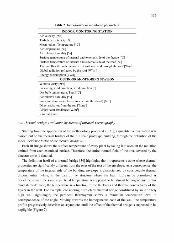
125

Table 2. Indoor-outdoor monitored parameters.

INDOOR MONITORING STATION Air velocity [m/s] Turbulence intensity [%] Mean radiant Temperature [°C] Air temperature [°C] Air relative humidity [%] Surface temperature of internal and external side of the façade [°C] Surface temperature of internal and external side of the roof [°C] Thermal flux through the north external wall and through the roof [W/m2] Global radiation reflected by the roof [W/m2] Energy consumption [kWh]

OUTDOOR MONITORING STATION Wind velocity [m/s] Prevailing wind direction, wind direction [°] Dry bulb temperature, Tout [°C] Air relative humidity [%] Sunshine duration (referred to a certain threshold) [0–1] Direct radiation from the sun [W/m2] Global solar irradiance [W/m2] Rain fall [mm]

3.2. Thermal Bridges Evaluation by Means of Infrared Thermography

Starting from the application of the methodology proposed in [31], a quantitative evaluation was carried out on the thermal bridges of the full scale prototype building, through the definition of the index Incidence factor of the thermal bridge Itb.

Each IR image shows the surface temperature of every pixel by taking into account the radiation emitted from each examined surface. Therefore, the entire thermal field of the area covered by the detector optic is detailed.

The definition itself of a thermal bridge [34] highlights that it represents a zone whose thermal properties are significantly different from the ones of the rest of the envelope. As a consequence, the temperature of the internal side of the building envelope is characterized by considerable thermal discontinuities, while, in the part of the structure where the heat flux can be considered as one-dimensional, the same superficial temperature is supposed to be almost homogeneous. In this “undisturbed” zone, the temperature is a function of the thickness and thermal conductivity of the layers in the wall. For example, considering a structural thermal bridge constituted by an infinitely high wall right-angle, the pertinent thermogram shows a minimum temperature level in correspondence of the angle. Moving towards the homogeneous zone of the wall, the temperature profile progressively describes an asymptote, until the effect of the thermal bridge is supposed to be negligible (Figure 2).

126

Figure 2. Example of an angular thermal bridge and relative thermogram output.

Itb is strongly linked to the temperature profile as it defines higher thermal losses in the pertinent zone of the building with respect to other homogeneous areas.

Equation (1) shows the mathematical meaning of the proposed index, describing the ratio between the thermal loss calculated from the measured temperature in the IR images and the hypothetical thermal loss of the same area in the wall, when calculated without considering the effect of thermal bridges.

)(

)(

)(

)(

)(

)(

_1

1_

_1

1_

_11_1

1__

isDi

N

pispixeli

isDipixel

N

pispixelipixel

isDiDiD

N

pispixelipixelitb

tb TTN

TT

TTNA

TTA

TTAh

TTAhI (1)

With the hypothesis of steady-state conditions and constant convective coefficient (htb_i = h1D_i), the index is the ratio between the temperature difference in the real case and in the hypothetical scenario where the thermal bridge effects are neglected.

The benefit of having both the temperature values in the two considered areas in one same IR image, i.e., the thermal bridge area and the homogeneous one, allows to minimize further sources of error related to non-contemporary measurements and to the influence produced by different viewed angles by the IR camera. Moreover, the capture of an only one IR image avoids the influence of the emissivity dependence from surface distance and angle of view. The ratio between the two fluxes considered in the definition of Itb, and in particular the direct definition of T1D_is from the thermogram, results useful to normalize the analysis, further simplifying experimental evaluations.

This quantitative phenomenon could also be described as a sort of increase in the thermal transmittance U1D of the undisturbed zone. Therefore, considering the thermal bridge effect, in the hypothesis of stationary conditions, the value of the thermal transmittance Utb can be written as follows (2):

tbDtb IUU 1 (2)

127

4. Discussion of the Results

4.1. Envelope Thermal Performance

A hypothetical specific heat loss through the test-room envelope was firstly assumed by neglecting the effect of thermal bridges. The thermal transmittance values were experimentally measured through the continuous monitored data. Non negligible differences between calculated and measured values were found, even if good thermal properties of the construction were observed.

The opaque envelope was divided in five areas with different thermal performance characteristics, without considering the effect of thermal bridges in the first phase of the analysis. The five areas consist of (i) vertical walls; (ii) roof; (iii) ground floor; (iv) door; and (v) window. The overall heat losses through the test-room resulted equal to 27.34 W/K. A time interval with relatively constant conditions, i.e., with relatively low effect of solar radiation and indoor thermal discontinuities, was chosen as reported in Figure 3. The overall heat losses parameter previously showed and the internal and external temperatures acquired during that period (10 h long interval) were useful to calculate the total energy heat losses value that corresponded to 4.349 kWh. Regarding the air infiltration losses, the standard exchange rate for natural ventilation of 0.3 volumes per hour was considered [35]. Therefore, the total thermal losses raised up to 30.11 W/K.

Figure 3. Thermal-energy profiles in the monitored period.

4.2. Analysis of Each Thermal Bridge Contribution

Firstly, each thermal bridge in the test-room building was classified and analyzed through IR imaging. The IR analyses allowed to identify the geometry and the area affected by the thermal bridge

128

with respect to the homogeneous zone. The identified thermal bridge typologies are reported as follows:

(1) Line between two walls (L-WW); (2) Corner between wall and roof (C-WR); (3) Corner between wall and ground floor (C-WG); (4) Line between wall and ground floor (L-WG); (5) Lines between clay elements and concrete elements in the roof ceiling structure (L-PT); (6) Line between wall and roof (L-WR); (7) Line between roof and wall (L-RW); (8) Lines between wall and door (L-WD); (9) Lines between wall and window (L-WI);

The evaluations of two thermal bridge typologies are reported in Figures 4 and 5. Figure 4 represents the temperature profile defining the horizontal thermal bridge between the ground floor and the wall. The thermal profile along the line where the incidence factor of the thermal bridge is calculated is reported in Figure 4b.

Figure 4. IR thermography and thermal profile of the thermal bridge between ground floor and wall [36].

The IR analysis showed an average indoor air temperature of 23 °C (Ti), while the temperature in the homogeneous areas of walls was around 21.4 °C (T1D_is). Equation 1 was used to calculate the proposed index, resulting equal to 1.52 in a 0.290 m long line between the wall and the ground floor. This index was then multiplied by the interested area of the wall and by the measured wall transmittance in the areas with no thermal bridge, in order to evaluate the total thermal loss by taking into account the thermal bridge effect.

Regarding the second thermal bridge, i.e., the corner between two walls and the roof ceiling, the increase of heat loss was identified in the influenced areas of every structural element affected by C-WR. Figure 5 reports the considered areas.

129

Figure 5. IR thermography of the C-WR thermal bridge and the relative area of influence.

In this case, the Incidence factor of the thermal bridge refers to the overall area, and not only to the line length. Table 3 reports the incidence factor values of the nine identified thermal bridges.

Table 3. Values of Incidence factor of the thermal bridge of each identified thermal bridge.

Thermal Bridge Itb L-WW 1.28 C-WR 2.15 C-WG 1.79 L-WG 1.52 L-PT 1.23 L-WR 1.53 L-RW 1.48 L-WD 1.44 L-WI -

The nine incidence factors of the thermal bridge show the strong relation between the geometry and the thermal performance of the structures. Analyzing the L-type thermal bridges, the low value of the indexes becomes evident when the discontinuity is just created by a geometrical thermal bridge (L-WW) or a change of the layer materials (L-PT). On the contrary, the effect of the thermal bridge is amplified where both the conditions are verified (i.e., L-WG, L-WR). The C-type thermal bridges show different values due to the elements that define the corner: the ground presents less thermal losses thanks to the different boundary conditions, therefore, the temperature values in the pertinent area of the floor show a lower temperature decrease and the index for the C-WR thermal bridge results higher than the C-WG thermal bridge. The thermal bridge L-WI was considered to be negligible, since the IR analysis showed a good quality of the execution of these technical elements, with non-significant thermal deviations between the window and the wall along the line.

130

4.3. Combined Assessment of in-Field Thermal-Energy Performance

The Itb calculation for each thermal bridge of the prototype building allowed to evaluate the overall conductance of the envelope. An influence area was assigned to each thermal bridge in order to identify an extra transmittance value to each of these areas. Figure 6 reports the example of the wall area influence by the thermal bridges. The same method was applied to the others surfaces of the test-room to assign each Itb previous showed in Table 3.

Figure 6. Thermal bridges influence scheme (section of the test-room).

The total thermal losses through the envelope of the prototype building, including the thermal bridges correspond to 32.73 W/K, where the heat transfer directly imputable to the thermal bridges presence is about 9%.

These values were compared to the energy consumption of the heat pump system operating in the test-room. In particular, the Coefficient of Performance of the system was calculated according to EN 14825 [37] in partial load conditions, and it corresponded to 2.6. In the selected period (Figure 3) the heat pump consumed 2.058 kWhel, corresponding to 5.272 kWhth.

Table 4 reports the heat pump energy consumption with and without considering the effect of thermal bridges, and the real measured consumption. The measured values show the substantial reliability of the proposed index. In fact, after a laboratory validation reported in previous works of the authors [31], the Incidence factor of the thermal bridge seems to be valid also in a real full-scale environment like the analyzed test-room. Table 4 reports the uncertainty values analyzed for each calculation and measurement according to [38].

Table 4. Comparison between energy consumption values in different approaches.

Energy Consumption without Thermal Bridges

[kWh]

Energy Consumption with Thermal Bridges

[kWh]

Measured Energy Consumption of the Heat Pump System

[kWh] 4.816 ± 0.082 5.258 ± 0.100 5.272 ± 0.527

Difference (%) 9.2% 0.3%

131

In particular, the uncertainty of the energy consumption in the configuration with thermal bridges takes into account the singular error due to the analysis of every thermal bridge. For matter of safety, each temperature pixel corresponds to an accuracy level of ±2 °C, in order to take into account of all possible uncertainties in the measurement procedures. Moreover, the results of this evaluation show that the quantitative thermography analysis lead to a reliable assessment of the real behavior of thermal bridges. In general, the effect of these particular building elements is evaluated through numerical calculations and dedicated software [17,39], producing results often far from the ones obtained experimentally. The whole technique is simple to use thanks to the thermographic survey that allows one to acquire images in a relatively easy and quick manner. As shown before, the calculation of the proposed index has to be carried out with the elaboration of one single thermographic image for each thermal bridge. The sole recommendation is that the IR image has to include both the thermal bridge area and the thermally homogeneous wall. Finally the elaboration of the temperature data of the thermogram, and the calculation of the Itb, is generally possible by means of common worksheets because the output of the thermo camera is a simple vector or matrix of temperature data. In this view, the proposed methodology could constitute a relatively easy to be applied and reliable analysis tool, with the purpose to evaluate the increase of thermal losses imputable to thermal bridges by means of in-situ measurements.

5. Conclusions

IR thermography represents an acknowledged qualitative methodology aimed at investigating thermal discontinuities throughout buildings envelope and the presence-positioning of thermal bridges. In this view, recent research efforts were aimed at developing quantitative techniques to analyze the effect of thermal bridges on building thermal-energy behavior. A quantitative index, i.e., the Incidence factor of the thermal bridge, was proposed in a previous work by the authors in order to quantify thermal losses through building envelopes. Starting from previous results, this work concerned the application and a further experimental in-field validation of the proposed index methodology in a full-scale continuously monitored building. Thermal bridges within the prototype building were identified and assessed through the proposed procedure. Continuous monitoring of indoor air temperature, surface temperature and thermal fluxes throughout the wall, the ground floor and the roof, allowed to compare the thermography results to quantitative monitored data. The analysis showed that the overall effect of thermal bridges in increasing thermal losses through the building envelope corresponded to about 9%. Moreover, the evaluation of the energy consumption of the operating heat pump system in heating mode and the survey of the overall thermal losses through the building envelope by means of the proposed index have been compared and the variation between these two approaches resulted lower than 1%. The geometrical simplicity of the case study building could be considered as a simplifying factor for the comparison between measured and calculated values. Future developments of this research will deal with a real operating building. Nevertheless, the proposed Incidence factor of the thermal bridge methodology confirmed to be an useful and relatively simple tool even in realistic in-field conditions, thanks to the reliable estimation of each thermal bridge correction factor.

132

Acknowledgments

The authors acknowledge “Fondazione Cassa di Risparmio Perugia” for funding the construction of the test room within the BAIO project.


The authors contributed equally to this work.

Nomenclature

Itb Incidence factor of the thermal bridge [-] htb_i Convective coefficient of the thermal bridge zone [W/m2K] h1D_i Convective coefficient of the undisturbed zone [W/m2K] Apixel Surface of the single pixel [m2] A1D Surface of the entire thermografic image [m2] Ti Temperature of the inner air [K] Tpixel_is Temperature of the single pixel on the surface [K] T1D_is Temperature of the surface on undisturbed zone defined by thermogram [K] N Total number of pixels U1D Thermal transmittance of the undisturbed zone [W/m2K] Utb Thermal transmittance of the zone influenced by thermal bridge [W/m2K]



References

1. Pikas, E.; Thalfeldt, M.; Kurnitski, J. Cost optimal and nearly zero energy building solutions for office buildings. Energy Build. 2014, 74, 30–42.

2. Asdrubali, F.; Baldassarri, C.; Fthenakis, V. Life cycle analysis in the construction sector: Guiding the optimization of conventional Italian buildings. Energy Build. 2013, 64, 73–89.

3. Franzitta, V.; Milone, A.; Milone, D.; Pitruzzella, S.; Trapanese, M.; Viola, A. Experimental evidence on the thermal performance of opaque surfaces in Mediterranean climate. Adv. Mater. Res. 2014, 860–863, 1227–1231.

4. Carletti, C.; Gallo, P.; Gargari, C.; Sciurpi, F. Building regulations based on sustainable principles in Italy: State of the art and trends. WIT Trans. Ecol. Environ. 2005, 84, 193–200.

5. Fantozzi, F.; Leccese, F.; Salvadori, G.; Tuoni, G. Energy demand analysis and energy labelling of new residential buildings in Tuscany (Italy). WIT Trans. Ecol. Environ. 2009, 122, 217–229.

6. De Lieto Vollaro, R.; Demegni, G.; Carnielo, E.; Botta, F.; de Lieto Vollaro, E. Determination of photometric properties of materials for energy purposes through the experimental study of a two-axis goniophotometer. Int. J. Eng. Technol. 2013, 5, 4465–4471.

133

7. Bottillo, S.; de Lieto Vollaro, A.; Galli, G.; Vallati, A. CFD modeling of the impact of solar radiation in a tridimensional urban canyon at different wind conditions. Sol. Energy 2014, 102, 212–222.

8. Carletti, C.; Cellai, G.; Sciurpi, F. Adapting prescriptions for energy saving technologies to historical buildings. In Proceedings of the 2nd Rebuild European Conference, Florence, Italy, 1–3 April 1998; pp. 290–293.

9. Pisello, A.L.; Asdrubali, F. Human-based energy retrofits in residential buildings: A cost-effective alternative to traditional physical strategies. Appl. Energy 2014, 133, 224–235.

10. Dutil, Y.; Rousse, D.; Quesada, G. Sustainable buildings: An ever evolving target. Sustainability 2011, 3, 443–464.

11. Cotana, F.; Rossi, F.; Filipponi, M.; Coccia, V.; Pisello, A.L.; Bonamente, E.; Petrozzi, A.; Cavalaglio, G. Albedo control as an effective strategy to tackle Global Warming: A case study. Appl. Energy 2014, doi:10.1016/j.apenergy.2014.02.065.

12. De Lieto Vollaro, R.; Calvesi, M.; Battista, G.; Evangelisti, L.; Gori, P.; Guattari, C. A new method of technical analysis to optimise the design of low impact energy systems for buildings. Int. J. Eng. Technol. Innov. 2013, 3, 241–250.

13. Franzitta, V.; Milone, D.; Trapanese, M.; Viola, A.; Di Dio, V.; Pitruzzella, S. Energy and economic comparison of different conditioning system among traditional and eco-sustainable building. Appl. Mech. Mater. 2013, 394, 289–295.

14. Galli, G.; Vallati, A.; Recchiuti, C.; de Lieto Vollaro, R.; Botta, F. Passive cooling design options to improve thermal comfort in an Urban District of Rome, under hot summer conditions. Int. J. Eng. Technol. 2013, 5, 4495–4500.

15. Ciampi, M.; Leccese, F.; Tuoni, G. Multi-layered walls design to optimize building-plant interaction. Int. J. Therm. Sci. 2004, 43, 417–429.

16. Brás, A.; Gonçalves, F.; Faustino, P. Cork-based mortars for thermal bridges correction in a dwelling: Thermal performance and cost evaluation. Energy Build. 2014, 72, 296–308.

17. Theodosiou, T.G.; Papadopoulos, A.M. The impact of thermal bridges on the energy demand of buildings with double brick wall constructions. Energy Build. 2008, 40, 2083–2089.

18. Ascione, F.; Bianco, N.; de Masi, R.F.; Vanoli, G.P. Rehabilitation of the building envelope of hospitals: Achievable energy savings and microclimatic control on varying the HVAC systems in Mediterranean climates. Energy Build. 2013, 60, 125–138.

19. Ghaffarianhoseini, A.; Dahlan, N.D.; Berardi, U.; Ghaffarianhoseini, A.; Makaremi, N.; Ghaffarianhoseini, M. Sustainable energy performances of green buildings: A review of current theories, implementations and challenges. Renew. Sustain. Energy Rev. 2013, 25, 1–17.

20. Rossi, F.; Pisello, A.L.; Nicolini, A.; Filipponi, M.; Palombo, M. Analysis of retro-reflective surfaces for urban heat island mitigation: A new analytical model. Appl. Energy 2014, 114, 621–631.

21. Asdrubali, F.; Baldinelli, G.; Bianchi, F. Influence of cavities geometric and emissivity properties on the overall thermal performance of aluminum frames for windows. Energy Build. 2013, 60, 298–309.

134

22. La Rosa, A.D.; Recca, A.; Gagliano, A.; Summerscales, J.; Latteri, A.; Cozzo, G.; Cicala, G. Environmental impacts and thermal insulation performance of innovative composite solutions for building applications. Constr. Build. Mater. 2014, 55, 406–414.

23. Baldinelli, G.; Asdrubali, F.; Baldassarri, C.; Bianchi, F.; D’Alessandro, F.; Schiavoni, S.; Basilicata, C. Energy and environmental performance optimization of a wooden window: A holistic approach. Energy Build. 2014, 79, 114–131.

24. Corgnati, S.P.; D’Oca, S.; Fabi, V.; Andersen, R.K. Leverage of behavioural patterns of window opening and heating set point adjustments on energy consumption and thermal comfort in residential buildings. Lect. Notes Electr. Eng. 2014, 261, 23–31.

25. Balaras, C.A.; Argiriou, A.A. Infrared thermography for building diagnostics. Energy Build. 2002, 34, 171–183.

26. Barreira, E.; de Freitas, V.P. Evaluation of building materials using infrared thermography. Constr. Build. Mater. 2007, 21, 218–224.

27. Avdelidis, N.P.; Moropoulou, A. Emissivity considerations in building thermography. Energy Build. 2002, 35, 663–667.

28. Datcu, S.; Ibos, L.; Candau, Y.; Matteï, S. Improvement of building wall surface temperature measurements by infrared thermography. Infrared Phys. Technol. 2005, 46, 451–467.

29. Zalewski, L.; Lassue, S.; Rousse, D.; Boukhalfa, K. Experimental and numerical characterization of thermal bridges in prefabricated building walls. Energy Convers. Manag. 2010, 51, 2869–2877.

30. Déqué, F.; Ollivier, F.; Roux, J.J. Effect of 2D modelling of thermal bridges on the energy performance of buildings—Numerical application on the Matisse apartment. Energy Build. 2001, 33, 583–587.

31. Asdrubali, F.; Baldinelli, G.; Bianchi, F. A quantitative methodology to evaluate thermal bridges in buildings. Appl. Energy 2012, 97, 365–373.

32. Pisello, A.L.; Cotana, F.; Nicolini, A.; Buratti, C. Effect of dynamic characteristics of building envelope on thermal-energy performance in winter conditions: In field experiment. Energy Build. 2014, doi:10.1016/j.enbuild.2014.05.017.

33. Barreneche, C.; de Gracia, A.; Serrano, S.; Navarro, M.E.; Borreguero, A.M.; Fernández, A.I.; Carmona, M.; Rodriguez, J.F.; Cabeza, L.F. Comparison of three different devices available in Spain to test thermal properties of building materials including phase change materials. Appl. Energy 2013, 109, 421–427.

34. International Organization for Standardization (ISO). Thermal Bridges in Building Construction—Linear Thermal Transmittance—Simplified Methods and Default Values; EN ISO 14683: 2008; ISO: Geneva, Switzerland, 2008.

35. Ente Nazionale Italiano di Unificazione (UNI). Prestazioni Energetiche Degli Edifici—Parte 1: Determinazione del Fabbisogno di Energia Termica dell’Edificio per la Climatizzazione Estiva ed Invernale; UNI/TS 11300–1: 2008; UNI: Milano, Italy, 2008.

36. Flir System. User’s Manual; Flir System: Wilsonville, OR, USA, 2008.

135

37. Air Conditioners, Liquid Chilling Packages and Heat Pumps, with Electrically Driven Compressors, for Space Heating and Cooling—Testing and Rating at Part Load Conditions and Calculation of Seasonal Performance; UNI EN 14825: 2012; BSI: London, UK, 2012.

38. International Organization for Standardization (ISO). Guide to the Expression of Uncertainty in Measurement; ENV 13005: 2008; ISO: Geneva, Switzerland, 2008.

39. Evola, G.; Margani, G.; Marletta, L. Energy and cost evaluation of thermal bridge correction in Mediterranean climate. Energy Build. 2011, 43, 2385–2393.

136

Numerical Study of Urban Canyon Microclimate Related to Geometrical Parameters

Andrea de Lieto Vollaro, Giuseppe de Simone, Roberto Romagnoli, Andrea Vallati and Simone Botillo

Abstract: In this study a microclimate analysis on a particular urban configuration: the—street canyon—has been carried out. The analysis, conducted by performing numerical simulations using the finite volumes commercial code ANSYS-Fluent, shows the flow field in an urban environment, taking into account three different aspect ratios (H/W). This analysis can be helpful in the study on urban microclimate and on the heat exchanges with the buildings. Fluid-dynamic fields on vertical planes within the canyon, have been evaluated. The results show the importance of the geometrical configuration, in relation to the ratio between the height (H) of the buildings and the width (W) of the road. This is a very important subject from the point of view of “Smart Cities”, considering the urban canyon as a subsystem of a larger one (the city), which is affected by climate changes.

Reprinted from Sustainability. Cite as: de Lieto Vollaro, A.; de Simone, G.; Romagnoli, R.; Vallati, A.; Botillo, S. Numerical Study of Urban Canyon Microclimate Related to Geometrical Parameters. Sustainability 2014, 6, 7894–7905.

1. Introduction

Thermal conditions in street canyons are important topics of urban microclimate, which influence the building’s energy demand and have a large impact on thermal comfort and on the health of people [1]. The reduction of energy consumption in buildings is a priority in the objectives “20-20-20” in the field of energy efficiency and Directive 2010/31/EU falls into this desire by offering guidelines for the Member States relating to the provision efficiency of buildings [2,3]. Surface temperature distribution and air circulation play an important role in heat exchange between the building and canyon air, which in turn influences pedestrian comfort and the energy demand of buildings. The landscape of dense urban areas can be described by units of street delimited by two continuous rows of buildings to form a “canyon”. Several studies have been performed on different street canyons, through numerical simulations [4,5], wind tunnel experiments [6], measurement campaigns [7,8] and pollution transport studies [9–14], the impact of surface heating on the flow field and on the exchange has been analyzed. The design of an urban canyon, defined as a stretch of road, relatively narrow and bounded on both sides in the longitudinal direction by continuous buildings, has a key role for the outdoor thermal comfort. It is a function of geometrical parameters, such as the average height H of the buildings facing on the roadway, the width W and the length L of the canyon. These parameters can affect the exchange of air mass and they can increase the concentration of pollutants generated by different human activities such as vehicular traffic and the heating of buildings. Also, the ratio of height to width and the canyon orientation affect the timing and magnitude of the energy regime of urban surfaces, which in particular influence the air temperature within the canyon. The study [15] focused on radiation fluxes, shows the importance of the shading towards the reduction of the radiant

137

heat gained from human body when compared to a person standing in a fully exposed location. Other studies [5,6,8,16–18] highlight the importance of canyon geometry in outdoor thermal comfort, which depends on the short and long-wave radiation fluxes from the entire surroundings of human beings. The goal of this study is to analyze how the flow field structure is affected by the H/W ratio and the effects of the heating of the façades on several planes of interest within the canyon, the evaluation of tridimensional effects on the flow field has been carried out. The analysis of the flow field within the canyon has been conducted with computational fluid dynamics (CFD) simulations performed during summer days, because, during this period, weather conditions affect human activity much more than during the winter season. The thermal field is induced by setting up the solar radiation module, the ambient conditions and thermo physical properties values of the buildings and the ground.

2. CFD Numerical Model

In this section the CFD numerical model that we have used to perform the simulations, is outlined. Further details on numerical model and on boundary conditions, not discussed in this paper, are listed in other papers [19] in which are used the same settings of CFD numerical model. Using the commercial CFD code ANSYS Fluent 14.0 [20], 3D double precision, pressure based version, the steady Reynolds-averaged Navier-Stokes (RANS) equations have been solved in combination with the standard k- model; the governing equations can be expressed as follows:

(1)

(2)

(3)

where is the average speed of air flow; is the Reynolds stress; is the air density; is the molecular viscosity; is the thermal-induced buoyant force; is the potential temperature; is the heat diffusivity. The standard k- model has been used to solve the turbulence problem. The standard k- model produces, as a result, an excessive turbulent kinetic energy in fluxes with considerable strong recirculating motions. However, in [21], various turbulence model are tested and it’s shown that more advanced models when compared with the standard k- model do not lead to relevant improvement, when the flow field has a significant longitudinal component. The turbulence kinetic energy, , and its rate of dissipation, , are obtained from the following transport equations:

(4)

(5)

where is the generation of turbulence kinetic energy due to the mean velocity gradients; is the generation of turbulence kinetic energy due to buoyancy; , constants and the and

138

expressions are reported in the standard k- model of ANSYS Fluent 14.0.0 [20]; and are the turbulent Prandtl numbers for and , respectively.

The degree to which is affected by the buoyancy is determined by the constant C3 . In ANSYS Fluent [20], C3 is not specified, but is instead calculated according to the following relation:

(6)

where is the component of the flow velocity parallel to the gravitational vector and u is the component of the flow velocity perpendicular to the gravitational vector [5]. To evaluate the impact of thermal effects, the natural convection module has been activated by setting incompressible ideal gas model for air density. Based on the best practice guidelines by Franke et al. [22] and Tominaga et al. [23], the computational domain has been extended beyond the built area by 5H in the North, West and South direction, of 15H in the East direction. The upper boundary condition is located at distance of 5H above the building roofs. These dimensions have been chosen to take into account of the blockage ratio and to ensure the flow re-development behind the building region. The temperature surfaces has been obtained as result of the heat transfer calculations, setting up: the solar load module, the temperature of undisturbed air (303 K), and the internal temperature of buildings (299 K). To simulate the ground influence, the computational domain has been extended 5 m below the ground level. The ground has been simulated setting the following parameters: density = 1000 kg/m3; specific heat = 1000 J/kg·K; thermal conductivity = 2 W/m·K; temperature at

5 m = 288 K; emissivity = 0.9; solar radiation absorptivity (direct visible and infrared) = 0.8. The radiation exchanges has been evaluated setting up the S2S radiation model, in which the energy exchange parameters are accounted by a geometric function, i.e., view factor, and activating the solar ray tracing in the solar load model, provided in ANSYS Fluent version 14.0.0. Transient heat conduction in ground and walls has been analyzed in [19]. This study finds that these effects are important to calculate heat fluxes, but not for surface temperatures which influence the natural convection flow fields. Furthermore, the materials characteristics have been reported in [22,23]: i.e., the building walls have: density = 1000 kg/m3; specific heat = 1000 J/kg·K; thermal conductivity = 0.15 W/m·K; thickness = 0.30 m; internal air temperature = 299 K; emissivity = 0.9; solar radiation absorptivity (direct visible and near infrared) = 0.8. To ensure a high quality of the computational grid, it is fully structured and the shape of the cells has been chosen hexahedral. The velocity profile has been set giving a uniform velocity magnitude at the velocity inlet boundary, the turbulence intensity at 10% and the roughness length . As the flow approaches the built area the velocity inlet profile is fully-developed before reaching the buildings [19] and it can be represented by Equation (7), where is the friction velocity, is the Von Karman constant (0.4) and z is the height coordinate. This equation represents the wind velocity profile of the inlet flow, when the wind approaches the buildings. In another study [19], it is shown that the profile reaches the asymptotic velocity when it reaches about 4 m in height.

139

The aerodynamic roughness value z0 has been set in relation to the roughness parameters in the ground surface boundary conditions (Ramponi and Blocken [24]): the sand-grain roughness height Ks and the roughness constant Cs. According to the best practices guideline for the CFD simulations by Franke et al. [22] and Tominaga et al. [23], setting Ks = 1 m and Cs = 0.5, we obtain z0 = 0.05 m (Blocken et al. [25], ANSYS Fluent User’s Guide [20]), that has been considered an appropriate value to represent the roughness of the outer region (Blocken et al. [25], Norris and Richards [26]).

(7)

The friction velocity value has been obtained by the correlation with the calculated value of the turbulent kinetic energy ( ) at the first node above the ground, as shown in Equation (8) [22].

(8)

where .

3. Results

The impact of H/W ratio and thermal effects on thermo fluid dynamics parameters has been studied performing six simulations on three street canyon models characterized by H/W = 0.5, 1, 2 respectively (Figure 1). The canyons are placed in Milan (longitude: 9.18, latitude: 45.47, UTC: +1) and their orientation is North/South. They are flanked by identical buildings having the following dimensions: height (H) = 20 m, length (L) = 100 m and three different widths (Wb) = 40m; 20 m and 10 m, in Figure 2 we can observe the computational domain. The flow regime impacting on the built area is described by a velocity inlet magnitude of 2 m/s and a wind direction of 45° N. The simulations have been performed in steady case at two different hours of the day: 11:00 and 14:00 of 21 July, as given by the software meteorological file, so that at 11:00 the windward façade is in shadow, instead at 14:00 it is exposed to sun radiation. For an isolated 3D street canyon, the three dimensional effect of the flow is evident in the formation of a spiral flow, produced by the combination of the downward vertical vortex and the longitudinal component of the wind velocity, as reported in other 3D simulations [21,27,28]; they found that the wind field in urban areas is quite complex and the simulated wind speed intensities can be totally different from the measured data. To evaluate the impact of H/W ratio on the thermal and flow field within the canyon, three vertical planes of interest between the buildings have been considered: North, Central and South plane, placed respectively at 10 m from the north opening, in the middle of the canyon and at 10 m from south opening. The analysis has been conducted graphically, evaluating velocity vectors on the planes of interest. In Figures 3–5 are reported the XZ velocity vectors on the three planes of interest at 11:00 and 14:00, for H/W = 0.5, 1, 2 respectively. The leeward façade (westerly building) is on the left side of the figures, instead the windward façade (easterly building) is on the right side. For simulations performed at 11:00, the flow pattern changes significantly from the north opening to the Central plane, instead, from the Central plane to the South one, the flow pattern remains basically constant (Figures 3a1,b1,c1, 4a1,b1,c1 and 5a1,b1,c1). At the North plane the flow field structure is the same for the two hours considered, for each H/W street canyons. In particular, the flow field is

140

characterized by an aerodynamic vortex in the upper corner of the plane, near the leeward façade (Figures 3a1,a2, 4a1,a2 and 5a1,a2). This vortex is generated by geometrical discontinuities (the roof and the vertical corner of the left building) and its axis is parallel to the canyon direction. From Central plane to the South plane, the aerodynamic vortex coming from the roof is fully-formed and it occupies all the space between buildings.

Figure 1. Views of the computational grids of the street canyons: H/W = 0.5 (a); 1 (b); 2 (c).

Figure 2. View of the computational domain.

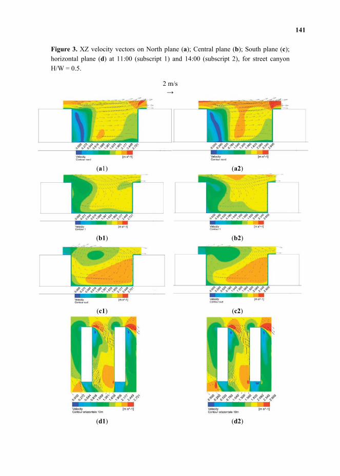
141

Figure 3. XZ velocity vectors on North plane (a); Central plane (b); South plane (c); horizontal plane (d) at 11:00 (subscript 1) and 14:00 (subscript 2), for street canyon H/W = 0.5.

2 m/s

(a1) (a2)

(b1) (b2)

(c1) (c2)

(d1) (d2)

142

Figure 4. XZ velocity vectors on North plane (a); Central plane (b); South plane (c); horizontal plane (d) at 11:00 (subscript 1) and 14:00 (subscript 2), for street canyon H/W = 1.

2 m/s

(a1) (a2)

(b1) (b2)

(c1) (c2)

(d1) (d2)

143

Figure 5. XZ velocity vectors on North plane (a); Central plane (b); South plane (c); horizontal plane (d) at 11:00 (subscript 1) and 14:00 (subscript 2), for street canyon H/W = 2.

2 m/s

(a1) (a2)

(b1) (b2)

(c1) (c2)

(d1) (d2)

144

Figure 6. XZ air temperature on Central plane for street canyon H/W = 2 (a); H/W = 1 (b); H/W = 0.5 (c), at 11:00 (subscript 1) and 14:00 (subscript 2).

(a1) (a2)

(b1) (b2)

(c1) (c2)

As the leeward facade is exposed to sun radiation, the natural convection gives a positive contribution to this spiral vortex coming from the roof. For the simulations performed at 14:00, in the Central and South plane the flow pattern is divided in two counter-rotating vortex: the upper one due to the geometrical discontinuity and the second one, due to the buoyancy effect, in the low corner near the hot wall. The convective vortex appears less developed than the simulations carried out by Li et al. [4] and Xie et al. [5], probably because of the 3D nature of our simulations. The impact of the natural convection vortex on the flow field structure, grows with the H/W ratio. As it can be seen in Figure 3(c2), when H/W = 0.5, even if the windward façade is sun-heated, the flow field structure between the buildings is strongly characterized by the large aerodynamic vortex and the buoyancy conducted vortex occupies the area near the hot wall which extends up to half height of the building. The same result is obtained for the simulations relative to H/W = 1; at 11:00 the aerodynamic vortex occupies all the space between the buildings (Figure 4c1), instead, at 14:00, the flow field is double-vortex in structure (Figure 4c2). When the height of the buildings doubles the width of the canyon (H/W = 2) and when the windward façade is sun-heated, the flow structure is strongly affected by the natural convection vortex. As it can be seen from a comparison between Figure 5b1,b2 and c1,c2, in the Central and South Plane, the natural convection vortex occupies a large part of area between the buildings. In particular, in the South Plane, while at 11:00 (Figure 5c1) the aerodynamic

145

vortex occupies all the area, at 14:00 it is almost absent and the motion due to buoyancy forces clearly prevails.

The phenomena of flow fields shown, as expected, dependent on the air temperature inside the canyon, as can be seen from Figure 6. In particular, the effect of temperature on the flow field within the canyon is most evident in Figure 5b2, where the formation of two vortices is a direct result of the air temperature rise near the leeward façade.

4. Conclusions

In this study a numerical simulation method has been used to investigate the physical phenomena that characterize the flow field structure within a street canyon, N-S oriented, during a summer day. A fully 3D model has been simulated, considering the effects of solar radiation and radiative exchange on canyon air and surfaces temperature, at two different hours of the day: 11:00 and 14:00. The importance of considering a 3D domain has been shown, because the flow field within the canyon changes significantly as the air passes through the canyon itself. When the windward façade is sun-heated, even if the flow field is characterized by a strong velocity component parallel to the canyon direction (direction: 45° N and intensity: 2 m/s), it has been noticed that the buoyancy force determines a thermal induced vortex near the hottest façade. Considering the natural convection effects, the flow field is complex, and it is strongly different for the two hours of the day considered. The impact of buoyancy forces on the flow field structure for three different H/W ratios, has been evaluated. In particular it has been shown that the impact of natural convection vortex, when the windward façade is sun-heated, increases with the H/W ratio. When the leeward façade is heated, instead, it has been shown that the flow pattern is characterized only by the aerodynamic vortex coming from the roof and, in these cases, the upward motion due to the buoyancy forces gives a positive contribution to the above mentioned vortex. Further analysis must be performed to quantify the effects of buoyancy forces on thermo fluid dynamic parameters, such as the convective heat transfer coefficient, turbulent kinetic energy, local values of velocity magnitude and surfaces temperatures.


Andrea de Lieto Vollaro and Andrea Vallati designed this research; Giuseppe De Simone and Roberto Romagnoli performed the calculations, analyzed the data and wrote the paper; Simone Botillo has revised the paper in English language. All authors have read and approved the final manuscript.



References

1. Moonen, P.; Defraeye, T.; Dorer, V.; Blocken, B.; Carmeliet, J. Urban physics effect of the micro-climate on comfort, health and energy demand. Front. Archit. Res 2012, 1, 197–228.

146

2. Asdrubali, F.; Bonaut, M.; Battisti, M.; Venegas, M. Comparative study of energy regulations for buildings in Italy and Spain. Energy Build. 2008, 40, 1805–1825.

3. Asdrubali, F.; Presciutti, A.; Scrucca, F. Development of a greenhouse gas accounting GIS-based tool to support local policy making—Application to an Italian municipality. Energy Policy 2013, 61, 587–594.

4. Li, L.; Yang, L.; Zhang, L.-J.; Jiang, Y. Numerical study on the impact of ground heating and ambient wind speed on flow fields in street canyons. Adv. Atmos. Sci. 2012, 29, 1227–1237.

5. Xie, X.; Liu, C.H.; Leung, D.Y.C. Impact of building facades and ground heating on wind flow and pollutant transport in street canyons. Atmos. Environ. 2007, 41, 9030–9049.

6. Uehara, K.; Murakami, S.; Oikawa, S.; Wakamatsu, S. Wind tunnel experiments on how thermal stratification affects how in and above urban street canyons. Atmos. Environ. 2000, 34, 1553–1562.

7. Offerle, B.; Eliasson, I.; Grimmond, C.S.B.; Holmer, B. Surface heating in relation to air temperature, wind and turbulence in an urban street canyon. Bound.-Layer Meterol. 2007, 122, 273–292.

8. Louka, P.; Vachon, G.; Sini, J.F.; Mestayer, P.G.; Rosant, J.M. Thermal effects on the airflow in a street canyon—Nantes’99 experimental results and model simulations. Water Air Soil Pollut. Focus 2002, 2, 351–364.

9. Li, X.-X.; Britter, R.E.; Koh, T.-Y.; Norford, L.K.; Liu, C.-H.; Entekhabi, D.; Leung, D.Y.C. Large-eddy simulation of flow and pollutant transport in urban street canyons with ground heating. Bound.-Layer Meteorol. 2010, 137, 187–204.

10. Li, X.-X.; Britter, R.E.; Norford, L.K.; Koh, T.-Y.; Entekhabi, D. Flow and pollutant transport in urban street canyons of different aspect ratios with ground heating: Large-eddy simulation. Bound.-Layer Meteorol. 2012, 142, 289–304.

11. Allegrini, J.; Dorer, V.; Carmeliet, J. Wind tunnel measurements of buoyant flows in street canyons. Build. Environ. 2013, 59, 315–326.

12. Park, S.-B.; Baik, J.-J.; Raasch, S.; Letzel, M.O. A large-eddy simulation study of thermal effects on turbulent flow and dispersion in and above a street canyon. J. Appl. Meteorol. Climatol. 2012, 51, 829–841.

13. Qu, Y.; Milliez, M.; Musson-Genon, L.; Carissimo, B. Numerical study of the thermal effects of buildings on low-speed airflow taking into account 3D atmospheric radiation in urban canopy. J. Wind Eng. Ind. Aerodyn. 2012, 104, 474–483.

14. Cai, X.-M. Effect of wall heating on flow characteristics in a street canyon. Bound.-Layer Meteorol. 2012, 142, 443–467.

15. Pearlmutter, D.; Bitan, A.; Berliner, P. Microclimatic analysis of “compact” urban canyons in an arid zone. Atmos. Environ. 1999, 33, 4143–4150.

16. Mayer, H.; Höppe, P. Thermal comfort of man in different urban environments. Theor. Appl. Climatol. 1987, 38, 43–49.

17. Mayer, H. Urban bioclimatology. Experientia 1993, 49, 957–963.

147

18. Kovar-Panskus, A.; Moulinneuf, L.; Savory, E.; Abdelqari, A.; Sini, J.F.; Rosant, J.M.; Robins, A.; Toy, N. A wind tunnel investigation of the influence of solar-induced wall-heating on the flow regime within a simulated urban street canyon. Water Air Soil Pollut. Focus 2002, 2, 555–571.

19. Bottillo, S.; de Lieto Vollaro, A.; Galli, G.; Vallati, A. Fluid dynamic and heat transfer parameters in an urban canyon. Sol. Energy 2013, 99, 1–10.

20. ANSYS Fluent, version 14.0.0; finite volumes software for the calculation of flow fields through the simulation within a virtual environment; ANSYS, Inc.: Canonsburg, PA, USA, 2011.

21. Assimakopoulos, V.D.; Georgakis, C.; Santamouris, M. Experimental validation of a computational fluid dynamics code to predict the wind speed in street canyons for passive cooling purposes. Sol. Energy 2006, 80, 423–434.

22. Franke, J.; Hellsten, A.; Schlunzen, H.; Carissimo, B. Best Practice Guideline for the CFD Simulation of Flows in the Urban Environment; COST Action 732; COST Office: Brussels, Belgium, 2007.

23. Tominaga, Y.; Mochidab, A.; Yoshiec, R.; Kataokad, H.; Nozue, T.; Yoshikawaf, M.; Shirasawac, T. AIJ guidelines for practical applications of CFD to pedestrian wind environment around buildings. J. Wind Eng. Ind. Aerodyn. 2008, 96, 1749–1761.

24. Ramponi, R.; Blocken, B. CFD simulation of cross-ventilation for a generic isolated building: Impact of computational parameters. Build. Environ. 2012, 53, 34–48.

25. Blocken, B.; Stathopoulos, T.; Carmeliet, J. CFD simulation of the atmospheric boundary layer: Wall function problems. Atmos. Environ. 2007, 41, 238–252.

26. Richards, P.J.; Norris, S.E. Appropiate boundary conditions for computational wind engineering models revisited. J. Wind Eng. Ind. Aerodyn. 2010, 99, 257–266.

27. Santamouris, M.; Papanikolaou, N.; Koronakis, I.; Livada, I.; Asimokopoulos, D. Thermal and air flow characteristics in a deep pedestrian canyon under hot weather conditions. Atmos. Environ. 1999, 33, 4503–4521.

28. Bottillo, S.; de Lieto Vollaro, A.; Galli, G.; Vallati, A. CFD modeling of the impact of solar radiation in a tridimensional urban canyon at different wind conditions. Sol. Energy 2014, 102, 212–222.

148

Linear, Non-Linear and Alternative Algorithms in the Correlation of IEQ Factors with Global Comfort: A Case Study

Francesco Fassio, Aldo Fanchiotti and Roberto de Lieto Vollaro

Abstract: Indoor environmental quality (IEQ) factors usually considered in engineering studies, i.e., thermal, acoustical, visual comfort and indoor air quality are individually associated with the occupant satisfaction level on the basis of well-established relationships. On the other hand, the full understanding of how single IEQ factors contribute and interact to determine the overall occupant satisfaction (global comfort) is currently an open field of research. The lack of a shared approach in treating the subject depends on many aspects: absence of established protocols for the collection of subjective and objective measurements, the amount of variables to consider and in general the complexity of the technical issues involved. This case study is aimed to perform a comparison between some of the models available, studying the results of a survey conducted with objective and subjective method on a classroom within University of Roma TRE premises. Different models are fitted on the same measured values, allowing comparison between different weighting schemes between IEQ categories obtained with different methods. The critical issues, like differences in the weighting scheme obtained with different IEQ models and the variability of the weighting scheme with respect to the time of exposure of the users in the building, identified during this small scale comfort assessment study, provide the basis for a survey activity on a larger scale, basis for the development of an improved IEQ assessment method.

Reprinted from Sustainability. Cite as: Fassio, F.; Fanchiotti, A.; de Lieto Vollaro, R. Linear, Non-Linear and Alternative Algorithms in the Correlation of IEQ Factors with Global Comfort: A Case Study. Sustainability 2014, 6, 8113–8127.

1. Introduction

The Indoor Environment Quality (IEQ) and the Comfort level to be guaranteed to building occupants, become essential factors to take in account when developing an efficient building design. This importance is testified both by the development of experimental sustainability assessment methods such as the SBTool [1], which, among others categories does take in account building occupant’s global comfort, by the design standards now available, such as EN 15251 [2], or by the reward value that environmental certification protocols, such as LEED (Leadership in Energy and Environmental Design), BREEAM (Building Research Establishment Environmental Assessment Methodology), ITACA (Innovazione e Trasparenza degli Appalti e Compatibilità Ambientale) and others, assign to a design exercise that takes into account these factors. It must be highlighted that in recent years the building industry has been giving a priority track to energy saving technologies, both through the development of technological systems with high energy efficiency [3], and promoting the issue of fit for purpose national regulations/standards [4]; less attention was devoted to IEQ improvement and associated monitoring procedures. This has been reflected also in recent versions

149

of environmental certification protocols like LEED v2009, as Watson [5] reported and as Altomonte et al. [6] analyzed in particular with respect to IEQ satisfaction by the users.

This is most probably linked to the fact that investments that generate energy savings can be more easily justified from the financial point of view and can be more easily implemented in a design strategy with respect to improvement in IEQ, where uniformly accepted classification and monitoring procedure are yet not established. Among others, Watson, in a more recent analysis [7], was reporting an average increase of 5% in the productivity of the personnel inside US commercial buildings LEED certified where IEQ was improved, while Wargocki et al. [8], among many other different studies, correlate the poor internal air quality with the Sick Building Syndrome (SBS) and decrease of productivity.

Even if the correlation between the IEQ and the occupants’ productivity is still an argument of discussion, establishing procedures and effective methods of evaluation of the IEQ is in any case an attractive field of research that is investigated in literature with different approaches. Heinzerling et al. [9] conducted a literature survey on the different method of evaluation of IEQ, highlighting how the currently available methods can be based on a combination of subjective and objective measures or are based on objective measurements made and compared against a fixed set of criteria that determine what assessment class the measurement falls into. Relevant consideration with respect to the available evaluation criteria are that:

• No uniform standards to perform objective measurements are available, both in terms of time and space rendering,

• Different IEQ factors weighting schemes and assessment class are proposed, • Inter-category relationships between IEQ factors are not considered, • Assessment scales considered are variable.

The diversity of the issues involved in the considerations above encourages the development of research programs that can give a contribution in defining standards procedure for the assessment and monitoring of IEQ in the build environment. The final aim of such research should be to define procedures that can join the “energy saving driven” design process with a “global comfort driven” one.

In [9], different IEQ factors weighting schemes available in literature, related to office spaces, are compared. However, the different models are not compared on the same survey database, neither uniform criteria of evaluation nor acceptance can be associated to the different methods. Scope of this preliminary case study is to set the procedures for a comparative study between different IEQ factors weighting methods, based on a single survey database.

In accordance with the approach used by most of the environmental certification protocols, the method shall be defined for a specific building type (residential, commercial, etc.). For the development of this study, a specific building category is considered, i.e., university training spaces. The selected type of environment provides a larger sample of simultaneous users per sqm, allowing, when considering user surveys in a single space, to collect more reliable observation from the statistical point of view.

150

2. IEQ Factors Evaluation: Objective and Subjective Method

The number of factors considered when assessing IEQ is variable. Common practice in standard engineering studies is to take in account four parameters, i.e., the thermal, acoustical, visual comfort, and the air quality.

Some studies, such as [10–12], take into account many additional parameters, related to ergonomics and overall internal environment (available space, privacy, furniture, finishing, cleanness, etc.) or other social/psychological/cultural factors, which certainly do have effects on the global comfort assessment by the users but are not part of the scope of work of this study.

The evaluation of comfort level in a building with respect to the four factors considered in this study, can be achieved through objective or subjective measurements:

An objective measurement consists in the collection of physical values for one or more parameters associated to each single IEQ factor (globe temperature, air speed, air temperature, humidity for thermal comfort, illuminance for visual comfort, concentration of CO2, CO and PMtot for air quality, weighted A equivalent continuous noise level for acoustical comfort, etc.). Such measurements can be taken with variable space and time rendering, depending on the aim of the study.

A subjective measurement is a survey performed through questionnaires where the assessment of different factors and overall satisfaction level is obtained directly through the opinion of the users. As for the objective measurements, time variable and user distribution in the building (space variable) are to be considered.

The two type of measurements generate two different main methods in assessing the IEQ:

Subjective-objective method: objective measurements are combined with subjective measurements using experimental models. Such models are based on equation that correlates the number of satisfied occupants with a physical value for each IEQ parameter (the coefficients of such equations are obtained through experimental data fitting). The number of satisfied occupants for each IEQ category is combined (with an experimental weighting scheme) to calculate an overall satisfaction index. Such an index is used to assess the space or building comfort against defined levels. Examples for such methods can be found in [13–17].

Objective criteria: objective measurements are compared with a fixed set of values, considering also for how long a value is observed to define in which category the space/building falls in with respect to a single IEQ factor or to the overall IEQ. In such an approach, subjective measurements can be collected (for validation) but are not part of the assessment process. Examples can be found in the method proposed by Marino et al. in [18] and similar.

The case study presented in this paper is aimed at comparing different subjective-objective methods, with particular focus on the models used to correlated single IEQ factors with overall occupant satisfaction, using the same sample of users, with simultaneous subjective and objective measurements.

151

This case study is aimed to set up a method of comparison using a small sample of users, allowing to define the procedures to be implemented in further research on a larger scale. The comparison will address the following aspects:

measurement procedures statistical significance of the coefficients obtained through data fitting procedures differences in the weighting schemes obtained with different models variability of the weighting scheme against the user's time of exposure in the building

The case study is focused on comfort assessment in classroom/training spaces, but useful references are obtained also from studies developed for different type of buildings, such as office spaces; likewise the procedures of comparison used for classrooms, can be applied also for studies of different type of buildings.

3. IEQ Models

Within the development of reliable building comfort assessment methods, this paper is part of a study focused on models available to correlate the different IEQ factor with respect to the global comfort. As observed by Humphreys [19], it is possibly not the right approach to look for a universal weighting scheme that can describe the contribution that each single IEQ factor provides in determining the global comfort level, while more effective results could be obtained in one to one category comparison. Once specific conditions (climatic, building function, architectural) are set, having a weighting scheme can be useful in prioritizing building improvement interventions, or in continuous monitoring of building performances an additional application could be found checking variation on the weighting scheme during the building life cycle.

The models available in literature to correlate the single IEQ factors with the global comfort are based on algorithms where the single coefficient are obtained through numerical data fitting on subjective measurements database. Depending on the type of function selected to describe the relationship between single IEQ factors and global comfort, different algorithms are applicable.

3.1. Multivariate Linear Regression Algorithm

In case linear dependency is chosen, multivariate linear regression can be used to obtain the coefficient from a database, as in [20]. In such a model, the correlation between occupant satisfaction on the single IEQ factor and overall satisfaction can be expressed as:

(1)

where ×1, ×2, ×3, ×4 and y are respectively the occupant satisfaction against each single IEQ factor, and the overall satisfaction; b0, b1 … b4 are the correlation factors and e is an error due to the exclusion from the model of external factors. In order to define values of b0, b1 … b4 required by the model, and the consequent weighting scheme, a multivariate linear regression algorithm can be used, fitting the values of the coefficients on the database composed by the single occupant satisfaction values collected with subjective measurements. The algorithm used has the following form:

152

(2)

3.2. Multivariate Logistic Regression Algorithm

An alternative model takes in account a non linear dependency between IEQ factors and overall satisfaction, such the one used by Wong et al in [17], where a logistic distribution function is used, which can be expressed as follows (in the general forms where n parameters are considered):

(3)

in the specific case where n = 4 (and using alternative form):

(4)

In order to evaluate the coefficient of the equation above using a data fitting procedure, a different algorithm has to be used with respect to the linear case, due to the non-applicability of the homoskedasticity of residuals hypothesis. In this case the maximum likelihood method is used, starting from the logit form of the equation:

(5)

Without going into the details, the set of equations that allows to solve with respect to 0 … 4, can be obtained deriving the likelihood function and setting the equations equal to 0 (maximum). The set of equations has an open solution. The numerical solver available in standard software, such as MATLAB, allows to determine the values of 0 … 4 that better fit the model on a database of subjective measurements.

3.3. Multivariate Linear Regression Algorithm Based on Dummy Variables

An alternative approach is used by Kim and De Daer in [21], using a theory based on the Kano model for market analysis. In such a model, linear correlation function is used to link the single IEQ factors and overall satisfaction, but having each single IEQ factor associated with dummy variables (a variable which can be set only on 0–1 values). The Dummy variables assume the following values:

xi1 = 1 ; xi2 = 0 if the occupant is satisfied of the IEQ factor xi1 = 0 ; xi2 = 0 if the occupant is neutral on the IEQ factor xi1 = 0 ; xi2 = 1 if the occupant is NOT satisfied of the IEQ factor

With such hypothesis the correlation function can be written as follows:

(6)

where:

153

y = the overall satisfaction xij = dummy variable associated to the i-factor considered (j = 1, 2 for each i-factor) n = number of IEQ factors considered b0, b11, b12, …, bn1, bn2 = coefficient that can be determined through linear regression

(as described for standard linear correlation function)

This algorithm allows to obtain two separate coefficients for each single IEQ factor considered, which provide a weighting scheme both for negative and positive user’ advice. These coefficients are useful to identify symmetrical and asymmetrical effects that the single IEQ factor has on the overall satisfaction. Following the same wording proposed by Kano, the single factors can be classified as follows:

if bi1 = bi2 = Proportional factors (factors that affect the overall satisfaction in the same way, being the user advice positive or negative)

if bi1 > bi2 = Bonus factors (factors that affect positively the overall satisfaction when the user advice on IEQ factor is positive, while negative advice is not affecting the overall satisfaction)

if bi1 < bi2 = Basic factors (factors that affect negatively the overall satisfaction when the user advice on IEQ factor is negative while positive advice is not affecting the overall satisfaction)

This approach can be useful when a significant number of factors are considered, in order to have a quick overview on the effects that each single factor has on the overall satisfaction, and can provide guidance in defining convenient improvement strategies.

3.4. Alternative Algorithms

A promising approach to describe correlations could be found in the implementation of artificial neural networks (ANN). Small reference are available in literature, but some applicable results can be found in Sofoglu [22], where an ANN model is fitted on objective measurements, linking the concentration of a number of pollutants in office space with the observed frequency of occupants showing sick building syndrome symptoms per square meter. Extending the method, a similar approach could be used to correlate the single IEQ factors and overall satisfaction of the occupants with on-time objective measurements, provided that the ANN black box is populated with a sufficiently large data set.

4. Experimental Section: Case Study Description

As anticipated, the aim of this case study was to set the procedures to develop a large-scale study, both to collect subjective and objective measurements and to select effective methods of comfort assessments based on such measurements. The test set up and procedures are described below.

4.1. Objective Measurements Test Set up

For the purpose of this small-scale case study, only one survey campaign has been performed and all measurements were taken in one single day, during the winter of 2013/2014 inside one classroom within the engineering faculty of the University of Roma Tre. The future development of the

154

large-scale study shall include both winter and summer measurements. During the survey, the outside temperature was 12 °C, partially cloudy, 65% humidity.

Within the university premises, and, in particular, in the classroom where the measurement were performed, the centralized air conditioning plant was operational. Figure 1 shows the localization of the space within the university premises and the measurement process performed together with subjective measurements.

An IEQ measurement station type BABUC A was used, collecting the values for air temperature, globe temperature, relative humidity, air speed, illuminance, CO and CO2 concentration, and weighted A equivalent continuous noise level.

The objective and subjective measurements were taken looking for two different time of exposure of the occupants, i.e., 15 min and 2 h (i.e., before and after an exam) in order to evaluate the variability of the survey results against time of exposure in a building coupled with the effect of the psychological stress caused by the exam on the users.

Figure 1. Measurement location.

4.2. Subjective Measurements

The sample was composed by 17 occupants. Questionnaires were distributed to the same sample at two different times, simultaneously with respect to objective measurements, in order to evaluate differences with respect to time of exposure. The questionnaires were collected immediately after completion in order to guarantee independency in the results. The questionnaire was obtained from the standard ISO 10551:1995, and is presented in Table 1.

155

Table 1. Questionnaire for subjective measurement.

With Respect to the categories on the right, DO YOU THINK THIS ENVORONMENT IS:

(choose one option only)

THERMAL COMFORT

ACOUSTIC COMFORT

VISUAL COMFORT

AIR QUALITY

GLOBAL COMFORT

Satisfactory (the activities can be properly

performed) 0 0 0 0 0

Not completely Tolerable 1 1 1 1 1 Hardly Tolerable 2 2 2 2 2

Unbearable 3 3 3 3 3

5. Results and Discussion

The results of the measurements collected and of the analysis performed on such database are discussed below. Taking in account the limited size of the sample considered, it is important to highlight that the quantitative result described hereinafter are not the aim of this study, which is basically devoted to identify useful inputs to develop the study on a larger scale.

5.1. Objective Measurements

The objective measurements collected are summarized in Tables 2 and 3. The tables presents the values of the different IEQ parameters measured in the four corners of the classroom, and the associated average values, with reference to the two different times of data collection, i.e., 9:45 am and 11:30 am. The measured IEQ parameters are: T (air temperature), Tdry (dry-bulb temperature), Thum (wet-bulb temperature), Urel (relative humidity), Tpr (dew point temperature), Tglob (globe temperature), Va (Air speed), Leq (weighted A equivalent continuous noise level), Lux (illuminance), CO2 (CO2 Concentration), and CO (CO concentration).

Table 2. Objective measurements at 9:45 am.

Survey Time: 9:45 am Objective Measurements Location: Corner 1 Corner 2 Corner 3 Corner 4 Average u.m.

T 24.11 24.57 24.72 24.45 24.46 C°

THERMAL

Tdry 25.06 24.83 24.95 24.07 24.73 C° Thum 16.09 16.2 16.54 16.12 16.24 C° Urel 36.60% 37.40% 37.20% 41.10% 38.08% % Tpr 9.12 9.43 9.6 9.93 9.52 C°

Tglob 23.77 23.01 24.16 23.84 23.70 C° Va 0.2 0.12 0.1 0.06 0.12 m/s Leq 71 66.4 70 63.6 67.75 dBa ACOUSTICAL Lux 360.00 lx VISUAL CO2 890.00 ppm

IAQ CO 1.40 mg/m3

156

Table 3. Objective measurements at 11:30 am.

Survey Time: 11:30 am Objective Measurements Location: Corner 1 Corner 2 Corner 3 Corner 4 Average u.m.

T 24.15 23.865 22.89 23.46 23.59 C°

THERMAL

Tdry 23.2 21.825 21.56 21.03 21.90 C° Thum 15.74 15.02 14.91 14.8 15.12 C° Urel 43.60% 46.70% 44.50% 49.50% 46.08% % Tpr 10.02 9.88 9.48 9.89 9.82 C°

Tglob 24 23.9 21.83 22.21 22.99 C° Va 0.05 0.085 0.05 0.04 0.06 m/s Leq 71 73 71 71 71.50 dBa ACOUSTICAL Lux 360.00 lx VISUAL CO2 950.00 ppm

IAQ CO 1.60 mg/m3

Based on this set of data, it would be possible to calculate the predicted percentage of dissatisfied users (separately with respect to the thermal environment, indoor air quality, aural environment and illumination level, at working plane) using equations available in literature, of which coefficients shall be obtained through a multivariate logistic regression data fitting procedure, based on a sufficiently large database of objective and subjective measurements. Such database is not available for the specific case, thus, just for procedure set up, the four equations proposed in [17] are used.

The four equations provide the percentage of satisfied users ( = 1, 2, 3, 4) with respect to each one of the four IEQ factors, against the value of selected parameters, namely:

Parameter 1 = PDD (calculated on the basis of the well-established standard [23]), for the thermal environment,

Parameter 2 = CO2 concentration, for the air quality (CO concentration is not considered), Parameter 3 = noise level in dba, for aural environment, Parameter 4 = illuminance in lux, for illumination level.

The coefficients of the four equations are fitted on measures collected in office spaces in Hong Kong. Even if the functions are not directly applicable to this case study, with the aim to set up a procedure, the level of acceptance of the IEQ factors is calculated using the measured values of IEQ parameters, in order to be compared with the results of the subjective survey, discussed below. The Results are summarized in Tables 4 and 5.

Table 4. Predicted percentage of Satisfied users–9:45 am.

9:45 am THERMAL IAQ ACOUSTICAL VISUAL

Parameter associated to Ieq Factor 1 2 3 4 U.m. PDD ppm dba lux

10.20 890.00 67.75 360.00 Predicted percentage of Satisfied users 1 2 3 4

0.90 0.94 0.61 0.73

157

Table 5. Predicted percentage of Satisfied users–11:30 am

11:30 am THERMAL IAQ ACOUSTICAL VISUAL

Parameter associated to Ieq Factor 1 2 3 4 U.m PDD ppm dba lux

8.30 950.00 71.50 360.00

Predicted percentage of Satisfied users 1 2 3 4

0.92 0.93 0.49 0.73

5.2. Subjective Measurement Results

Table 6 presents the distribution of the votes obtained from the questionnaires, with reference to each IEQ factor and overall satisfaction, in the two time frames.

Table 6. Distribution of the votes in subjective measurements.

Questionnaires 9:45 am VOTE THERMAL IAQ ACOUS. VISUAL GLOBAL

unbearable 3 0 1 0 0 0 hardly tolerable 2 1 0 4 0 1

not completely tolerable 1 2 3 6 1 3 Satisfactory (the activities can be

properly peformed) 0 14 13 7 16 13

AVERAGE 0.24 0.35 0.82 0.06 0.29 ST. DEV. 0.56 0.79 0.81 0.24 0.59

Questionnaires 11:30 am VOTE THERMAL IAQ ACOUS. VISUAL GLOBAL

unbearable 3 0 1 1 0 0 hardly tolerable 2 0 1 4 0 1

not completely tolerable 1 5 2 7 3 3 Satisfactory (the activities can be

properly peformed) 0 12 13 5 14 13

AVERAGE 0.29 0.41 1,06 0.18 0.29 ST. DEV. 0.47 0.87 0.90 0.39 0.59

With reference to the results of the questionnaires presented above, the following aspects can be highlighted:

In both the timeframes of sampling it results that the worst average vote (the higher the number, the worst is the level of satisfaction) is related to the aural environment. This result is also in accordance with the prediction presented in Tables 4 and 5, where it was shown that the lowest number of satisfied users was expected with respect to the noise level, both at 9:45 am and 11:30 am.

158

The predicted variation of satisfied users with respect to the conditions measured at 9:45 am and 11:30 am (see Tables 4 and 5) is quite in accordance with the variation of the Average vote obtained from the survey. A lack of accuracy can in any case justified by the fact that the equations used are not fitted on data base collected in the environment of this case study.

The average vote on global comfort does not change in the two timeframes considered, while the average vote against the different IEQ factors is variable. This means that weighting scheme that associates the level of satisfaction against the global comfort and single IEQ factors is variable with the time of exposure of the user in the building.

5.3. IEQ Weighting Scheme Comparison

The votes collected have been used to identify the coefficients in both the multivariate linear regression and the multivariate logistic regression algorithms, separately for each time frame. Weighting coefficients are standardized and normalized. The weighting schemes obtained are summarized in Table 7 and Figure 2.

Table 7. Weighting schemes obtained with multivariate linear and logistic regressions.

MULTIVARIATE LINEAR REGRESSION 9:45 am

x1-TERM x2-ACUS. x3-VISUAL x4-IAQ b1 b2 b3 b4

0.02 0.31 0.56 0.12 11:30 am

x1-TERM x2-ACUS. x3-VISUAL x4-IAQ b1 b2 b3 b4

0.33 0.18 0.38 0.10 MULTIVARIATE LOGISTIC REGRESSION

9:45 am x1-TERM x2-ACUS. x3-VISUAL x4-IAQ

k1 k2 k3 k4 0.33 0.26 0.25 0.16

11:30 am x1-TERM x2-ACUS. x3-VISUAL x4-IAQ

k1 k2 k3 k4 0.30 0.28 0.30 0.12

159

Figure 2. Weighting scheme obtained with linear and logistic regression algorithms.

In both cases, linear and logistic regression data fitting, did not provided coefficients with sufficient statistic reliability (in some cases p close to 1), which was expected due to the very small size of the sample. With similar processes, in the literature referenced above, good statistical reliability was obtained with samples composed of nearly, or more than, 300 occupants.

It can be noted that even if coefficients have different variability in the two models, logistic regression provide more similar values, while linear regression over/underestimate the values of the higher and smaller coefficients.

The weighting scheme shows a significant variability with respect to time of exposure, which again is even more amplified in the linear regression model. In any case, the inclusion in the model of coefficients which can take in account the time of exposure of the occupants to weight the vote seems a hypothesis to be investigated to take into account such variability in the results.

6. Conclusions

The analysis of the available literature shows that additional efforts are required in order to define effective occupant satisfaction and global comfort assessment methods. When available, such methods shall gain a similar relevance to energy saving procedures in the design process. Space and time rendering protocols shall be established in order to better compare and select the most appropriate procedures. With respect to the models used to correlate the single IEQ factors with

0.00

0.20

0.40

0.60

0.80

1.00x1 TERM

x2 ACUS.

x3 VISUAL

x4 IAQ

reg.LIN 9:45am reg.LIN 11:30am reg. LOG 9:45am reg.LOG 11:30am

160

overall occupant satisfaction, different approaches are available and new ones shall be developed. The weighting schemes between different IEQ categories obtained with such models, although not very useful to define a universal rule, can be considered an additional instrument to prioritize building interventions or to develop continuous monitoring procedures during the building life cycle.

The results obtained in this preparatory case study, provide some relevant information to develop a larger-scale survey and data analysis. The key issues identified are the following:

Subjective measurements sample size and models reliability—the coefficient of the models obtained with the data fitting are not always statistically reliable: in order to define a model with sufficient predictive ability, fitting the data on a larger sample (min 300 subjects) is required.

Structure of subjective measurements questionnaires—the number of questions for each IEQ factor tends to distort the weight of the factor with respect to the overall satisfaction. It is convenient to simplify the questionnaire used with a uniform set of questions: for each IEQ factor only acceptability—not acceptable shall be asked. As an option, these basic questions could be integrated, with a second set asking to provide a review of each factor using the ASHRAE (American Society of Heating, Refrigerating and Air Conditioning Engineers) scale (+3, 3).

Prediction of satisfied users against each single IEQ factor—the equations available in literature seem suitable to predict the level of satisfaction of the users for a given value of IEQ parameters, provided that a data fitting procedure is performed on a database populated with a set of measurements that covers all the typical conditions of the environment.

Correlation model comparisons—it was noted a significant variability in the coefficients obtained from the data set related to two different sampling times. The linear regression algorithm tends to overestimate the bigger coefficient, while the logistic regression coefficient is more stable. In this sense, the adoption of a non-linear model (as reg.log) appears more promising for IEQ factors and overall comfort correlation. The linear regression showed higher statistical reliability with respect to the logistic regression, which probably is due to the limited sample size.

Variability of the weighting scheme with respect to the time of exposure—the preliminary data obtained shows that the weighting scheme can be variable with the time of exposure of the users in the same indoor space. Further study shall address this point in order to investigate if correction coefficients associated to the time of exposure can efficiently take in account this aspect.

New correlation models—ANN network model has to be investigated. The inclusion of time dependency in the models should be investigated.

Acknowledgments

The authors would like to thank the students that participated to the survey and the University of Rome Tre for the possibility of performing the survey activities within its premises.

161


The research was designed and performed by Aldo Fanchiotti, Roberto de Lieto Vollaro and Francesco Fassio, while the data analysis and the paper drafting was performed by Francesco Fassio. All authors have read and approved the final manuscript.


The authors declare no conflict of interest

References

1. Mateus, R.; Bragança, L. Sustainability Assessment and Rating of Buildings: Developing the Methodology SBToolPT–H. Build. Environ. 2011, 46, 1962–1971.

2. Italian Organization for Standardization (UNI). Indoor Environmental Input Parameters for Design and Assessment of Energy Performance of Buildings Addressing Indoor Air Quality, Thermal Environment, Lighting and Acoustics; UNI EN 15251:2007; UNI: Milano, Italy, 2007.

3. Asdrubali, F.; Bonaut, M.; Battisti, M.; Venegas, M. Comparative Study of Energy Regulations for Buildings in Italy and Spain. Energy Build. 2008, 40, 1805–1825.

4. De Lieto Vollaro, A.; de Lieto Vollaro, R.; Peruzzi, L.; Salata, F. The reliability of technological systems with high energy efficiency in residential buildings. Energy Build. 2014, 68, 19–24.

5. Watson, R. Green Building Impact Report; GreenBiz Group Inc.: Oakland, CA, USA, 2008. 6. Altomonte, A.; Schiavon, S. Occupant satisfaction in LEED and non-LEED certified buildings.

Build. Environ. 2013, 68, 66–76. 7. Watson, R. Green Building Impact Report; GreenBiz Group Inc.: Oakland, CA, USA, 2011. 8. Wargocki, P.; Wyon, D.P.; Sundell, J.; Clausen, G.; Fanger, P.O. The effects of outdoor air

supply rate in an office on perceived air quality, sick building syndrome (SBS) symptoms and productivity. Indoor Air 2000, 10, 222–236.

9. Heinzerling, D.; Schiavon, S.; Webster, T.; Arens, E. Indoor environmental quality assessment models: A literature review and a proposed weighting and classification scheme. Build. Environ. 2013, 70, 210–222.

10. Bluyssen, P.M.; Janssen, S.H.; van den Brink, L.; de Kluizenaar, Y. Assessment of wellbeing in an indoor office environment. Build. Environ. 2011, 46, 2632–2640.

11. Bluyssen, P.M.; Aries, M.; van Dommelen, P. Comfort of workers in office buildings: The European HOPE project. Build. Environ. 2011, 46, 280–288.

12. Frontczak, M.; Wargocki, P. Literature survey on how different factors influence human comfort in indoor environments. Build. Environ. 2011, 46, 922–937.

13. Fanger, P.O. Thermal Comfort; McGraw Hill: New York, NY, USA, 1972. 14. Mui, K.W.; Wong, L.T. Neutral temperature in subtropical climates: A field survey in

air-conditioned offices. Build. Environ. 2007, 42, 699–706. 15. Mui, K.W.; Wong, L.T. Minimum acceptable noise level for office occupants. Build. Serv. Eng.

Res. Technol. 2006, 27, 249–254.

162

16. Mui, K.W.; Wong, L.T. Acceptable illumination level for office occupants. Archit. Sci. Rev. 2006, 49, 116–119.

17. Wong, L.T.; Mui, K.W.; Hui, P.S. A multivariate-logistic model for acceptance of indoor environmental quality (IEQ) in offices. Build. Environ. 2008, 43, 1–6.

18. Marino, C.; Nucara, A.; Pietrafesa, M. Proposal of comfort classification indexes suitable for both single environments and whole buildings. Build. Environ. 2012, 57, 58–68.

19. Humphreys, M.A. Quantifying occupant comfort: are combined indices of the indoor environment practicable? Build. Res. Inf. 2005, 33, 317–325.

20. Barbaro, S.; Ganci, A. Studio del comfort globale negli ambienti indoor. Applicazione alla facoltà di ingegneria dell’università’ di Palermo. Available online: http://www.cti2000.it/index.php?controller=pubblicazioni&action=show&id=29576 (accessed on 7 November 2014). (In Italian)

21. Kim, J.; de Dear, R. Nonlinear relationships between individual IEQ factors and overall workspace satisfaction. Build. Environ. 2012, 49, 33–40.

22. Sofuoglu, S.C. Application of artificial neural networks to predict prevalence of building-related symptoms in office buildings. Build. Environ. 2008, 43, 1121–1126.

23. International Organization for Standardization (ISO). Moderate Thermal Environments—Determination of the PMV and PPD Indices and Specification of the Conditions for Thermal Comfort; ISO 7730:1994. ISO: London, UK, 1994.

MDPI • Basel • Beijing • Wuhan Å BarcelonaISBN 978-3-03842-098-9www.mdpi.com

14th CIRIAF National Congress PDF final

Documents

Transcript of 14th CIRIAF National Congress PDF final