A new design method for retaining walls in clay

Ashraf S. Osman and Malcolm D. Bolton

Abstract: Geotechnical design engineers used to rely on arbitrary rules and definitions of “factor of safety” on peaksoil strength in limit analysis calculations. They used elastic stiffness for deformation calculations, but the selection ofequivalent linear elastic models was always arbitrary. Therefore, there is a need for a simple unified design method thataddresses the real nature of serviceability and collapse limits in soils, which always show a nonlinear and sometimesbrittle response. An approach to this method can be based on a new application of the theory of plasticity accompaniedby the introduction of the concept of “mobilizable soil strength.” This approach can satisfy both safety and serviceabil-ity and lead to simple design calculations within which all geotechnical design objectives can be achieved in a singlestep of calculation. The proposed method treats a stress path in an element, representative of some soil zone, as acurve of plastic soil strength mobilized as strains develop. Designers enter these strains into a plastic deformationmechanism to predict boundary displacements. The particular case of a cantilevered retaining wall supporting an exca-vation in clay is selected for a spectrum of soil conditions and wall flexibilities. The possible use of the mobilizablestrength design (MSD) method in decision-making and design is explored and illustrated.

Key words: retaining wall, plasticity theory, design, finite element.

Résumé : Les ingénieurs géotechniciens avaient l’habitude de se fier dans leurs calculs d’analyse limite à des règles etdéfinitions arbitraires du « coefficient de sécurité » basées sur la résistance de pic du sol. Ils utilisaient la rigidité élas-tique pour les calculs des déformations, mais la sélection de modèles équivalents élastiques linéaires était toujours arbi-traire. En conséquence, on a besoin d’une méthode simple et unifiée de conception qui traite de la nature réelle de lapraticabilité et des limites d’effondrement des sols, qui montre toujours une réponse non linéaire et parfois fragile. Uneapproche à cette méthode peut être basée sur une nouvelle application de la théorie de plasticité accompagnée del’introduction du concept de « résistance mobilisable du sol ». Cette approche peut satisfaire tant la sécurité que la pra-ticabilité, et peut conduire à des calculs simples de conception dans lesquels tous les objectifs de conception géotech-nique peuvent être atteints au cours d’une étape unique de calcul. La méthode proposée considère un cheminement decontrainte dans un élément représentatif d’une certaine zone de sol, comme étant une courbe de résistance plastique dusol mobilisée à mesure que les déformations se développent. Les concepteurs entrent ces déformations dans un méca-nisme de déformation plastique pour prédire les déplacements aux frontières. Le cas particulier d’un mur de soutène-ment en porte-à-faux retenant une paroi d’excavation dans l’argile a été choisi comme éventail des conditions des solset de la flexibilités du mur. On explore et illustre l’utilisation possible de la méthode de calcul de la résistance mobili-sable (MSD) pour la prise de décision et la conception.

Mots clés : mur de soutènement, théorie de plasticité, conception, éléments finis.

[Traduit par la Rédaction] Osman and Bolton 466

Introduction

Historically, plasticity theory has been used for calculat-ing the distribution of lateral earth pressure, which is thecentral issue in the analysis of retaining structures. In thistheory, a zone of soil is assumed to reach plastic equilibriumsuch that plastic collapse occurs. This plastic soil zone slipsrelative to the rest of the soil mass. The peak soil strength isassumed to be mobilized on the slip surface. The collapseload is then calculated and factors of safety are introduced toallow for uncertainties and to limit movements by ensuring

that the stresses are far from their ultimate values. Differentdefinitions of factors of safety are adopted in design codesand used in practice, however.

Code of practice (CP2)Bolton (1993) illustrates the mixture of definitions of fac-

tor of safety in the Code of practice for earth retainingstructures (CP2) (British Standards Institution 1994), whichwas first published in 1951. For a deep circular slip, a factorof safety of 1.25 is used and is defined as the restoring mo-ment divided by the overturning moment. For embeddedwalls, the limiting passive resultant is reduced by a factor of2, and the unfactored active value is used on the retainedside. This was pointed out by Hubbard et al. (1984) as tooconservative because, in certain design situations, a strongerand deeper wall is needed to achieve this arbitrary factor. Italso creates an inconsistency, since the factor of safety canactually decrease with an increase of wall penetration in un-drained conditions. Additionally, in drained conditions the

Can. Geotech. J. 41: 451–466 (2004) doi: 10.1139/T04-003 © 2004 NRC Canada

451

Received 29 April 2003. Accepted 5 December 2003.Published on the NRC Research Press Web site athttp://cgj.nrc.ca on 29 June 2004.

A.S. Osman1 and M.D. Bolton. Department of Engineering,Cambridge University, Trumpington Street, CambridgeCB2 1PZ, UK.

1Corresponding author (e-mail: aseko2@cam.ac.uk).

factor of safety has a finite value for zero height of retainedmaterial (Burland et al. 1981).

CIRIA report 104Construction Industry Research and Information Associa-

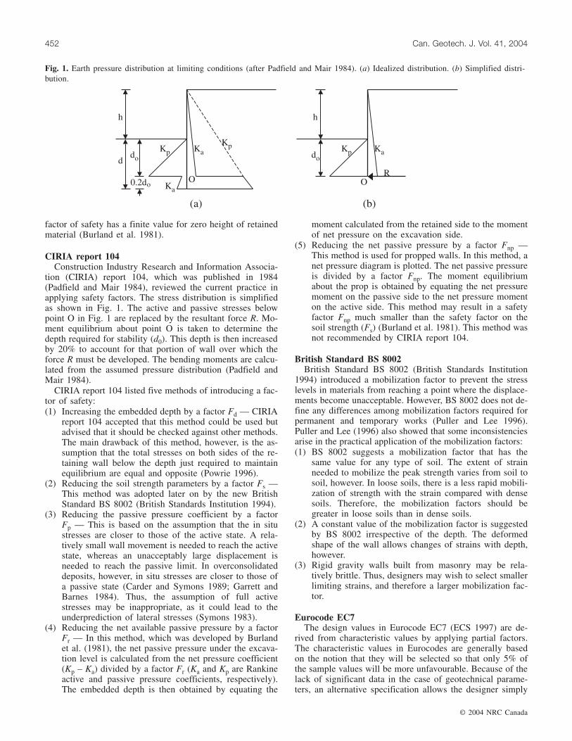
tion (CIRIA) report 104, which was published in 1984(Padfield and Mair 1984), reviewed the current practice inapplying safety factors. The stress distribution is simplifiedas shown in Fig. 1. The active and passive stresses belowpoint O in Fig. 1 are replaced by the resultant force R. Mo-ment equilibrium about point O is taken to determine thedepth required for stability (d0). This depth is then increasedby 20% to account for that portion of wall over which theforce R must be developed. The bending moments are calcu-lated from the assumed pressure distribution (Padfield andMair 1984).

CIRIA report 104 listed five methods of introducing a fac-tor of safety:(1) Increasing the embedded depth by a factor Fd — CIRIA

report 104 accepted that this method could be used butadvised that it should be checked against other methods.The main drawback of this method, however, is the as-sumption that the total stresses on both sides of the re-taining wall below the depth just required to maintainequilibrium are equal and opposite (Powrie 1996).

(2) Reducing the soil strength parameters by a factor Fs —This method was adopted later on by the new BritishStandard BS 8002 (British Standards Institution 1994).

(3) Reducing the passive pressure coefficient by a factorFp — This is based on the assumption that the in situstresses are closer to those of the active state. A rela-tively small wall movement is needed to reach the activestate, whereas an unacceptably large displacement isneeded to reach the passive limit. In overconsolidateddeposits, however, in situ stresses are closer to those ofa passive state (Carder and Symons 1989; Garrett andBarnes 1984). Thus, the assumption of full activestresses may be inappropriate, as it could lead to theunderprediction of lateral stresses (Symons 1983).

(4) Reducing the net available passive pressure by a factorFr — In this method, which was developed by Burlandet al. (1981), the net passive pressure under the excava-tion level is calculated from the net pressure coefficient(Kp – Ka) divided by a factor Fr (Ka and Kp are Rankineactive and passive pressure coefficients, respectively).The embedded depth is then obtained by equating the

moment calculated from the retained side to the momentof net pressure on the excavation side.

(5) Reducing the net passive pressure by a factor Fnp —This method is used for propped walls. In this method, anet pressure diagram is plotted. The net passive pressureis divided by a factor Fnp. The moment equilibriumabout the prop is obtained by equating the net pressuremoment on the passive side to the net pressure momenton the active side. This method may result in a safetyfactor Fnp much smaller than the safety factor on thesoil strength (Fs) (Burland et al. 1981). This method wasnot recommended by CIRIA report 104.

British Standard BS 8002British Standard BS 8002 (British Standards Institution

1994) introduced a mobilization factor to prevent the stresslevels in materials from reaching a point where the displace-ments become unacceptable. However, BS 8002 does not de-fine any differences among mobilization factors required forpermanent and temporary works (Puller and Lee 1996).Puller and Lee (1996) also showed that some inconsistenciesarise in the practical application of the mobilization factors:(1) BS 8002 suggests a mobilization factor that has the

same value for any type of soil. The extent of strainneeded to mobilize the peak strength varies from soil tosoil, however. In loose soils, there is a less rapid mobili-zation of strength with the strain compared with densesoils. Therefore, the mobilization factors should begreater in loose soils than in dense soils.

(2) A constant value of the mobilization factor is suggestedby BS 8002 irrespective of the depth. The deformedshape of the wall allows changes of strains with depth,however.

(3) Rigid gravity walls built from masonry may be rela-tively brittle. Thus, designers may wish to select smallerlimiting strains, and therefore a larger mobilization fac-tor.

Eurocode EC7The design values in Eurocode EC7 (ECS 1997) are de-

rived from characteristic values by applying partial factors.The characteristic values in Eurocodes are generally basedon the notion that they will be selected so that only 5% ofthe sample values will be more unfavourable. Because of thelack of significant data in the case of geotechnical parame-ters, an alternative specification allows the designer simply

© 2004 NRC Canada

452 Can. Geotech. J. Vol. 41, 2004

Fig. 1. Earth pressure distribution at limiting conditions (after Padfield and Mair 1984). (a) Idealized distribution. (b) Simplified distri-bution.

to select a cautious estimate for the characteristic value ap-propriate to occurrence of limit states. Having taken thisjudgment based on experience, the designer is instructed onthe precise partial factor by which soil strengths, for exam-ple, are reduced. This rationale is based on a rather vaguetreatment of the probability of exceedence of peak strengths.It does not address the problem of excessive displacements(Simpson and Driscoll 1998).

Mobilizable strength design (MSD) method

In current design practice, there is a distinction betweencalculations for safety requirements and calculations for dis-placements. Plasticity theory is used in collapse calculations,whereas elasticity theory is used to predict displacements.The stresses under working conditions, however, are farfrom those obtained by plasticity theory, which predictsstresses at failure. The applications of elasticity theory areoften complex and are based on an arbitrary equivalentmodulus. Codes of practice do not deal with serviceability inany great depth (Simpson and Driscoll 1998).

Therefore, there is a need for a simple unified design ap-proach that could relate successfully the real nature of ser-viceability and collapse limits to the soil behaviour. Boltonet al. (1989, 1990a, 1990b) proposed a new approach basedon the theory of plasticity accompanied by the introductionof the concept of “mobilizable soil strength.” The proposeddesign method treats a stress path in a representative soilzone as a curve of plastic soil strength mobilized as strainsdevelop. Strains are entered into a simple plastic deforma-tion mechanism to predict boundary displacements. Stressesare entered into simple equilibrium diagrams to demonstratestability. Hence, the proposed mobilizable strength design(MSD) method might satisfy both safety and serviceabilityin a single step of calculation.

This paper focuses on the undrained shearing of clays toillustrate the MSD approach. Clays that remain undrainedduring construction must deform only in shear, and engi-neers use a shear stress τ rising towards an undrained shearstrength cu to define the loading of the material towards fail-ure. To emphasise the concept that all shear stresses mobi-lize some shear strains, the symbol cmob is used instead of τand is referred to as the mobilized strength.

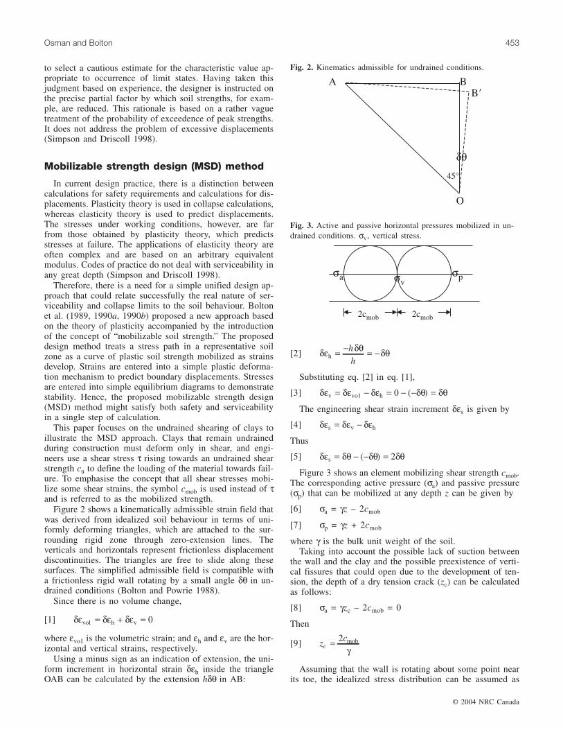
Figure 2 shows a kinematically admissible strain field thatwas derived from idealized soil behaviour in terms of uni-formly deforming triangles, which are attached to the sur-rounding rigid zone through zero-extension lines. Theverticals and horizontals represent frictionless displacementdiscontinuities. The triangles are free to slide along thesesurfaces. The simplified admissible field is compatible witha frictionless rigid wall rotating by a small angle δθ in un-drained conditions (Bolton and Powrie 1988).

Since there is no volume change,

[1] δε δε δε1vo h v= + = 0

where εvo1 is the volumetric strain; and εh and εv are the hor-izontal and vertical strains, respectively.

Using a minus sign as an indication of extension, the uni-form increment in horizontal strain δεh inside the triangleOAB can be calculated by the extension hδθ in AB:

[2] δε δθ δθh = − = −hh

Substituting eq. [2] in eq. [1],

[3] δε δε δε δθ δθv vo1 h= − = − − =0 ( )

The engineering shear strain increment δεs is given by

[4] δε δε δεs v h= −

Thus

[5] δε δθ δθ δθs = − − =( ) 2

Figure 3 shows an element mobilizing shear strength cmob.The corresponding active pressure (σa) and passive pressure(σp) that can be mobilized at any depth z can be given by

[6] σa = γz – 2cmob

[7] σp = γz + 2cmob

where γ is the bulk unit weight of the soil.Taking into account the possible lack of suction between

the wall and the clay and the possible preexistence of verti-cal fissures that could open due to the development of ten-sion, the depth of a dry tension crack (zc) can be calculatedas follows:

[8] σa = γzc – 2cmob = 0

Then

[9] zc

c = 2 mob

γ

Assuming that the wall is rotating about some point nearits toe, the idealized stress distribution can be assumed as

© 2004 NRC Canada

Osman and Bolton 453

Fig. 2. Kinematics admissible for undrained conditions.

Fig. 3. Active and passive horizontal pressures mobilized in un-drained conditions. σv, vertical stress.

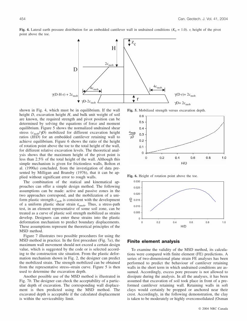
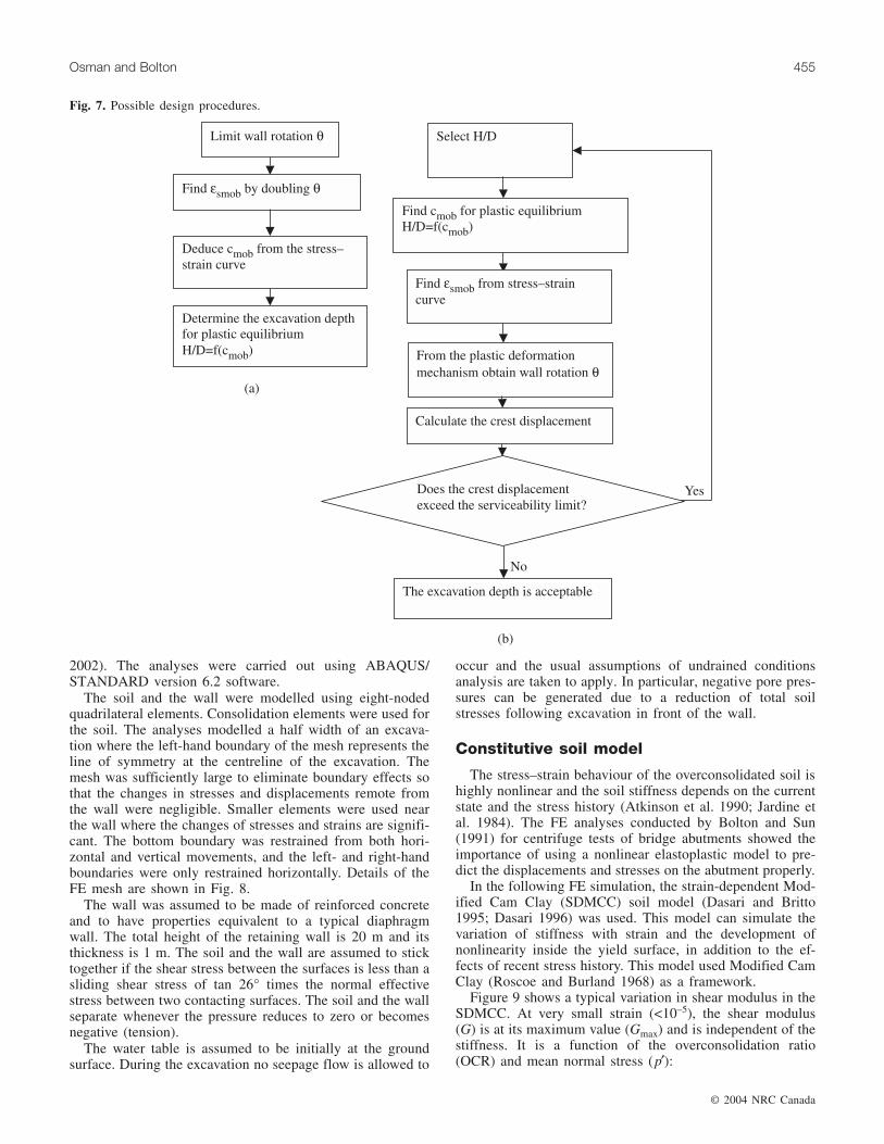
shown in Fig. 4, which must be in equilibrium. If the wallheight D, excavation height H, and bulk unit weight of soilare known, the required strength and pivot position can bedetermined by solving the equations of force and momentequilibrium. Figure 5 shows the normalized undrained shearstress (cmob/γD) mobilized for different excavation heightratios (H/D) for an embedded cantilever retaining wall toachieve equilibrium. Figure 6 shows the ratio of the heightof rotation point above the toe to the total height of the wall,for different relative excavation levels. The theoretical anal-ysis shows that the maximum height of the pivot point isless than 2.5% of the total height of the wall. Although thissimple mechanism is given for frictionless walls, Bolton etal. (1990a) concluded, from the investigation of data pre-sented by Milligan and Bransby (1976), that it can be ap-plied without significant error to rough walls.

The combination of the statical and kinematical ap-proaches can offer a simple design method. The followingassumptions can be made: active and passive zones in thetwo approaches correspond, and the mobilization of a uni-form plastic strength cmob is consistent with the developmentof a uniform plastic shear strain εsmob. Thus, a stress-pathtest, in an element representative of some soil zone, can betreated as a curve of plastic soil strength mobilized as strainsdevelop. Designers can enter these strains into the plasticdeformation mechanism to predict boundary displacements.These assumptions represent the theoretical principles of theMSD method.

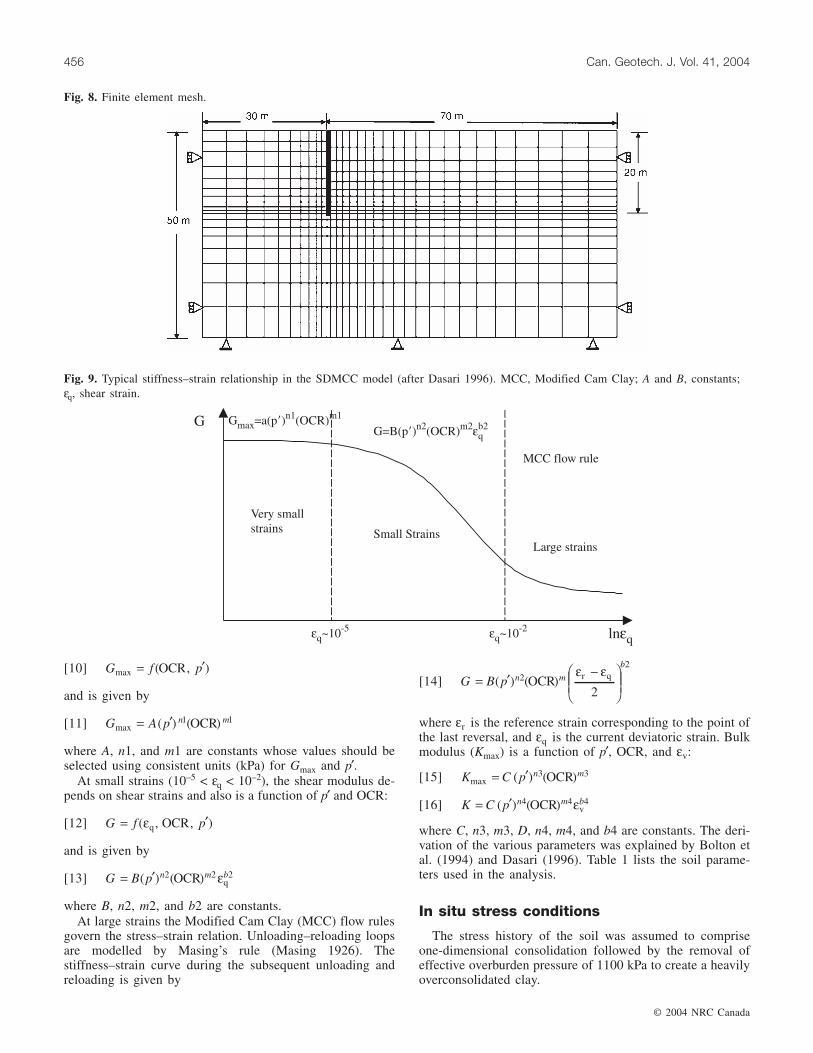
Figure 7 illustrates two possible procedures for using theMSD method in practice. In the first procedure (Fig. 7a), themaximum wall movement should not exceed a certain designvalue, which is suggested by the code or is selected accord-ing to the construction site situation. From the plastic defor-mation mechanism shown in Fig. 2, the designer can predictthe mobilized strain. The strength mobilized can be obtainedfrom the representative stress–strain curve. Figure 5 is thenused to determine the excavation depth.

Another possible use of the MSD method is illustrated inFig. 7b. The designer can check the acceptability of a partic-ular depth of excavation. The corresponding wall displace-ment is then predicted using the MSD method. Theexcavated depth is acceptable if the calculated displacementis within the serviceability limit.

Finite element analysis

To examine the validity of the MSD method, its calcula-tions were compared with finite element (FE) predictions. Aseries of two-dimensional plane strain FE analyses has beenperformed to predict the behaviour of cantilever retainingwalls in the short term in which undrained conditions are as-sumed. Accordingly, excess pore pressure is not allowed todissipate during the analysis. In all the analyses, it has beenassumed that excavation of soil took place in front of a pre-formed cantilever retaining wall. Retaining walls in softclays would certainly be propped or anchored near theircrest. Accordingly, in the following demonstration, the clayis taken to be moderately or highly overconsolidated (Osman

© 2004 NRC Canada

454 Can. Geotech. J. Vol. 41, 2004

Fig. 4. Lateral earth pressure distribution for an embedded cantilever wall in undrained conditions (K0 = 1.0). r, height of the pivotpoint above the toe.

Fig. 5. Mobilized strength versus excavation depth.

Fig. 6. Height of rotation point above the toe.

© 2004 NRC Canada

2002). The analyses were carried out using ABAQUS/STANDARD version 6.2 software.

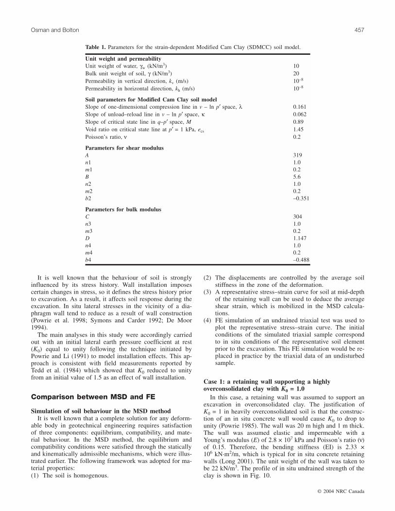
The soil and the wall were modelled using eight-nodedquadrilateral elements. Consolidation elements were used forthe soil. The analyses modelled a half width of an excava-tion where the left-hand boundary of the mesh represents theline of symmetry at the centreline of the excavation. Themesh was sufficiently large to eliminate boundary effects sothat the changes in stresses and displacements remote fromthe wall were negligible. Smaller elements were used nearthe wall where the changes of stresses and strains are signifi-cant. The bottom boundary was restrained from both hori-zontal and vertical movements, and the left- and right-handboundaries were only restrained horizontally. Details of theFE mesh are shown in Fig. 8.

The wall was assumed to be made of reinforced concreteand to have properties equivalent to a typical diaphragmwall. The total height of the retaining wall is 20 m and itsthickness is 1 m. The soil and the wall are assumed to sticktogether if the shear stress between the surfaces is less than asliding shear stress of tan 26° times the normal effectivestress between two contacting surfaces. The soil and the wallseparate whenever the pressure reduces to zero or becomesnegative (tension).

The water table is assumed to be initially at the groundsurface. During the excavation no seepage flow is allowed to

occur and the usual assumptions of undrained conditionsanalysis are taken to apply. In particular, negative pore pres-sures can be generated due to a reduction of total soilstresses following excavation in front of the wall.

Constitutive soil model

The stress–strain behaviour of the overconsolidated soil ishighly nonlinear and the soil stiffness depends on the currentstate and the stress history (Atkinson et al. 1990; Jardine etal. 1984). The FE analyses conducted by Bolton and Sun(1991) for centrifuge tests of bridge abutments showed theimportance of using a nonlinear elastoplastic model to pre-dict the displacements and stresses on the abutment properly.

In the following FE simulation, the strain-dependent Mod-ified Cam Clay (SDMCC) soil model (Dasari and Britto1995; Dasari 1996) was used. This model can simulate thevariation of stiffness with strain and the development ofnonlinearity inside the yield surface, in addition to the ef-fects of recent stress history. This model used Modified CamClay (Roscoe and Burland 1968) as a framework.

Figure 9 shows a typical variation in shear modulus in theSDMCC. At very small strain (<10–5), the shear modulus(G) is at its maximum value (Gmax) and is independent of thestiffness. It is a function of the overconsolidation ratio(OCR) and mean normal stress (p′):

Osman and Bolton 455

Fig. 7. Possible design procedures.

[10] G f pmax ( , )= ′OCR

and is given by

[11] G A p n mmax ( ) ( )= ′ 1 1OCR

where A, n1, and m1 are constants whose values should beselected using consistent units (kPa) for Gmax and p′.

At small strains (10–5 < εq < 10–2), the shear modulus de-pends on shear strains and also is a function of p′ and OCR:

[12] G f p= ′( , , )εq OCR

and is given by

[13] G B p n m b= ′( ) ( )2 2 2OCR qε

where B, n2, m2, and b2 are constants.At large strains the Modified Cam Clay (MCC) flow rules

govern the stress–strain relation. Unloading–reloading loopsare modelled by Masing’s rule (Masing 1926). Thestiffness–strain curve during the subsequent unloading andreloading is given by

[14] G B p n m

b

= ′ −

( ) ( )2

2

OCR2

r qε ε

where εr is the reference strain corresponding to the point ofthe last reversal, and εq is the current deviatoric strain. Bulkmodulus (Kmax) is a function of p′, OCR, and εv:

[15] K C p n mmax ( ) ( )= ′ 3 3OCR

[16] K C p n m b= ′( ) ( )4 4 4OCR vε

where C, n3, m3, D, n4, m4, and b4 are constants. The deri-vation of the various parameters was explained by Bolton etal. (1994) and Dasari (1996). Table 1 lists the soil parame-ters used in the analysis.

In situ stress conditions

The stress history of the soil was assumed to compriseone-dimensional consolidation followed by the removal ofeffective overburden pressure of 1100 kPa to create a heavilyoverconsolidated clay.

© 2004 NRC Canada

456 Can. Geotech. J. Vol. 41, 2004

Fig. 8. Finite element mesh.

Fig. 9. Typical stiffness–strain relationship in the SDMCC model (after Dasari 1996). MCC, Modified Cam Clay; A and B, constants;εq, shear strain.

It is well known that the behaviour of soil is stronglyinfluenced by its stress history. Wall installation imposescertain changes in stress, so it defines the stress history priorto excavation. As a result, it affects soil response during theexcavation. In situ lateral stresses in the vicinity of a dia-phragm wall tend to reduce as a result of wall construction(Powrie et al. 1998; Symons and Carder 1992; De Moor1994).

The main analyses in this study were accordingly carriedout with an initial lateral earth pressure coefficient at rest(K0) equal to unity following the technique initiated byPowrie and Li (1991) to model installation effects. This ap-proach is consistent with field measurements reported byTedd et al. (1984) which showed that K0 reduced to unityfrom an initial value of 1.5 as an effect of wall installation.

Comparison between MSD and FE

Simulation of soil behaviour in the MSD methodIt is well known that a complete solution for any deform-

able body in geotechnical engineering requires satisfactionof three components: equilibrium, compatibility, and mate-rial behaviour. In the MSD method, the equilibrium andcompatibility conditions were satisfied through the staticallyand kinematically admissible mechanisms, which were illus-trated earlier. The following framework was adopted for ma-terial properties:(1) The soil is homogenous.

(2) The displacements are controlled by the average soilstiffness in the zone of the deformation.

(3) A representative stress–strain curve for soil at mid-depthof the retaining wall can be used to deduce the averageshear strain, which is mobilized in the MSD calcula-tions.

(4) FE simulation of an undrained triaxial test was used toplot the representative stress–strain curve. The initialconditions of the simulated triaxial sample correspondto in situ conditions of the representative soil elementprior to the excavation. This FE simulation would be re-placed in practice by the triaxial data of an undisturbedsample.

Case 1: a retaining wall supporting a highlyoverconsolidated clay with K0 = 1.0

In this case, a retaining wall was assumed to support anexcavation in overconsolidated clay. The justification ofK0 = 1 in heavily overconsolidated soil is that the construc-tion of an in situ concrete wall would cause K0 to drop tounity (Powrie 1985). The wall was 20 m high and 1 m thick.The wall was assumed elastic and impermeable with aYoung’s modulus (E) of 2.8 × 107 kPa and Poisson’s ratio (ν)of 0.15. Therefore, the bending stiffness (EI) is 2.33 ×106 kN·m2/m, which is typical for in situ concrete retainingwalls (Long 2001). The unit weight of the wall was taken tobe 22 kN/m3. The profile of in situ undrained strength of theclay is shown in Fig. 10.

© 2004 NRC Canada

Osman and Bolton 457

Unit weight and permeabilityUnit weight of water, γw (kN/m3) 10Bulk unit weight of soil, γ (kN/m3) 20Permeability in vertical direction, kv (m/s) 10–8

Permeability in horizontal direction, kh (m/s) 10–8

Soil parameters for Modified Cam Clay soil modelSlope of one-dimensional compression line in v – ln p′ space, λ 0.161Slope of unload–reload line in v – ln p′ space, κ 0.062Slope of critical state line in q–p′ space, M 0.89Void ratio on critical state line at p′ = 1 kPa, ecs 1.45Poisson’s ratio, ν 0.2

Parameters for shear modulusA 319n1 1.0m1 0.2B 5.6n2 1.0m2 0.2b2 –0.351

Parameters for bulk modulusC 304n3 1.0m3 0.2D 1.147n4 1.0m4 0.2b4 –0.488

Table 1. Parameters for the strain-dependent Modified Cam Clay (SDMCC) soil model.

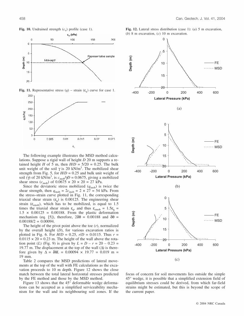
The following example illustrates the MSD method calcu-lations. Suppose a rigid wall of height D 20 m supports a re-tained height H of 5 m, then H/D = 5/20 = 0.25. The bulkunit weight of the soil γ is 20 kN/m3. The mobilized shearstrength from Fig. 5, for H/D = 0.25 and bulk unit weight ofsoil (γ) of 20 kN/m3, is cmob/γD = 0.0675, giving a mobilizedshear stress (cmob) of 0.0675 × 20 × 20 = 27 kPa.

Since the deviatoric stress mobilized (qmob) is twice theshear strength, then qmob = 2cmob = 2 × 27 = 54 kPa. Fromthe stress–strain curve plotted in Fig. 11, the correspondingtriaxial shear strain (εq) is 0.00125. The engineering shearstrain (εsmob), which has to be mobilized, is equal to 1.5times the triaxial shear strain εq, and thus εsmob = 1.5εq =1.5 × 0.00125 = 0.00188. From the plastic deformationmechanism (eq. [5]), therefore, 2δθ = 0.00188 and δθ =0.00188/2 = 0.00094.

The height of the pivot point above the toe (r), normalizedby the overall height (D), for various excavation ratios isplotted in Fig. 6. For H/D = 0.25, r/D = 0.0115. Thus r =0.0115 × 20 = 0.23 m. The height of the wall above the rota-tion point (L) (Fig. 9) is given by L = D – r = 20 – 0.23 =19.77 m. The displacement at the top of the wall (∆) is there-fore given by ∆ = δθL = 0.00094 × 19.77 = 0.019 m =19 mm.

Table 2 compares the MSD predictions of lateral move-ments at the top of the wall with FE calculations as the exca-vation proceeds to 10 m depth. Figure 12 shows the closematch between the total lateral horizontal stresses predictedby the FE method and those by the MSD method.

Figure 13 shows that the 45° deformable wedge deforma-tions can be accepted as a simplified serviceability mecha-nism for the wall and its neighbouring soil zones. If the

focus of concern for soil movements lies outside the simple45° wedge, it is possible that a simplified extension field ofequilibrium stresses could be derived, from which far-fieldstrains might be estimated, but this is beyond the scope ofthe current paper.

© 2004 NRC Canada

458 Can. Geotech. J. Vol. 41, 2004

Fig. 10. Undrained strength (cu) profile (case 1).

Fig. 11. Representative stress (q) – strain (εq) curve for case 1.

Fig. 12. Lateral stress distribution (case 1): (a) 5 m excavation,(b) 8 m excavation, (c) 10 m excavation.

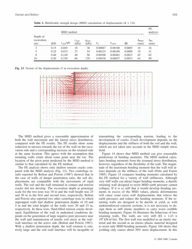
The MSD method gives a reasonable approximation ofboth the wall movement and the lateral stress distribution,compared with the FE results. The FE results show somereduction in stresses towards the toe of the wall on the exca-vation side and a corresponding increase on the retained sideat the same location. This agrees with the assumption thatretaining walls rotate about some point near the toe. Thelocation of the pivot point predicted by the MSD method issimilar to that calculated by the FE method.

The FE analysis shows only shallow tension cracks com-pared with the MSD analysis (Fig. 12). Two centrifuge re-sults reported by Bolton and Powrie (1987) showed that inthe case of walls of deeper penetration ratio, the soil dis-placements are compatible with the movements of rigidwalls. The soil and the wall remained in contact and tensioncracks did not develop. The excavation depth at prototypescale for the two tests was 10 m and the wall height was 25and 30 m in the first and second tests, respectively. Boltonand Powrie also reported two other centrifuge tests in whichunpropped walls had shallow penetration depths of 10 and5 m and the total heights of the walls were 20 and 15 m,respectively. In these tests, fluid-filled tension cracks devel-oped. Equilibrium of the wall in undrained conditions de-pends on the generation of large negative pore pressures nearthe wall and transmission of tensile soil stress at the soil–wall interface on the active side (Bolton and Powrie 1987).With a shallow penetration depth, the wall rotation is rela-tively large and the soil–wall interface will be incapable of

transmitting the corresponding tension, leading to thedevelopment of cracks. Crack development depends on thedisplacements and the stiffness of both the soil and the wall,which are not taken into account in the MSD simple stressfield.

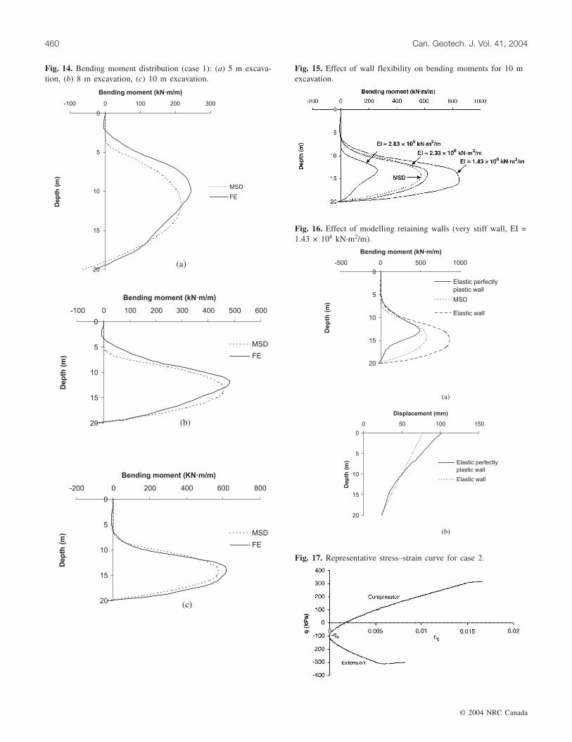
Figure 14 shows that MSD method can give reasonablepredictions of bending moments. The MSD method calcu-lates bending moments from the assumed stress distribution,however, regardless of the flexibility of the wall. The magni-tude of the maximum bending moment that the wall will at-tract depends on the stiffness of the wall (Potts and Fourie1985). Figure 15 compares bending moments calculated bythe FE method for a variety of wall stiffnesses. Althoughvery stiff walls can attract larger bending moments, a ductileretaining wall designed to resist MSD earth pressure cannotcollapse. If it is so stiff that it would develop bending mo-ments in excess of the MSD values, plastic deformationswill cause some extra wall displacements that relieve theearth pressures and reduce the bending moments. If the re-taining walls are designed to be ductile at yield, as withunderreinforced concrete sections, it is not necessary to de-sign them as stiff elastic members to carry worst crediblebending moments. Figure 16 illustrates the behaviour of tworetaining walls. The walls are very stiff (EI = 1.43 ×108 kN·m2/m). The first wall was modelled as an elastic ma-terial and the second as an elastic–plastic material designedto resist only MSD bending moments. Figure 16b shows thatyielding only causes about 20% more displacement. In this

© 2004 NRC Canada

Osman and Bolton 459

Fig. 13. Vectors of the displacements (5 m excavation depth).

MSD methodFEanalysis

Depth ofexcavation(m) H/D cmob/γD

cmob

(kPa)qmob

(kPa) εq εsmob δθ∆MSD

(mm)∆FE

(mm)

3 0.15 0.045 18 36 0.00067 0.00100 0.0005 10 165 0.25 0.075 27 54 0.00125 0.00188 0.0009 19 318 0.40 0.120 48 96 0.00308 0.00462 0.0023 45 62

10 0.50 0.150 60 120 0.00438 0.00657 0.0033 64 90

Table 2. Mobilizable strength design (MSD) calculations of displacements (K = 1.0).

© 2004 NRC Canada

460 Can. Geotech. J. Vol. 41, 2004

Fig. 14. Bending moment distribution (case 1): (a) 5 m excava-tion, (b) 8 m excavation, (c) 10 m excavation.

Fig. 15. Effect of wall flexibility on bending moments for 10 mexcavation.

Fig. 16. Effect of modelling retaining walls (very stiff wall, EI =1.43 × 108 kN·m2/m).

Fig. 17. Representative stress–strain curve for case 2.

case, designers will be relying on the durability of reinforcedconcrete where small cracks have occurred and where thesteel is at yield.

Case 2: a rigid wall supporting highly overconsolidatedclay with K0 = 2.0

In this case, the validity of MSD assumptions was exam-ined for a typical concrete wall supporting highly over-consolidated London clay, which somehow retains a K0value of 2.0.

The permissible stress field shown in Fig. 4 is inappropri-ate if the preexcavation earth pressure coefficient is notequal to unity, because some soil strength is being mobilizedon both sides of the wall before any wall movement takesplace. An alternative stress distribution can be derived asfollows. Consider a soil element at depth z below the ground

surface (assuming the water level is at the ground surface).The initial effective horizontal stress (σh′ ) can be approxi-mated by

[17] σ γ γh w′ = −K z0( )

where γ is the bulk unit weight of the soil, and γw is the unitweight of water. Thus, the total lateral pressure (σh) exertedon a frictionless rigid wall installed in the ground, prior toexcavation, is given by

[18] σ γ γ γh w w= − +K z z0( )

This equation can be rewritten in the form

[19] σ γ γ γh w= + − −z K z( ) ( )0 1

The vertical stress is given by

[20] σ γv = z

Therefore, prior to excavation, the soil with K0 ≠ 1.0 hasan initially mobilized deviator stress (qo) given by

[21] q K zo w= − −( ) ( )0 1 γ γ

The active pressure (σa) and passive pressure (σp) at anydepth z can then be given by

[22] σ γa o mob= + −z q c2∆

and

[23] σ γp p o mob= + +z q c2∆

where ∆cmob is the change of mobilized strength induced bywall movement, z is the depth measured from the groundlevel, and zp is measured from the excavation level. Thevalue qo merely increases all the stresses and reduces thedepth of tension. The depth of a dry tension crack (zc) canbe calculated by

[24] zc

Kc

mob

w

=+ − −

210

∆γ γ γ( ) ( )

In this case study, the constitutive model used in FE anal-ysis happened to give an identical change of stress versuschange of strain for compression and extension stress pathsin the nonlinear elastic zone. This was because of the adop-tion of isotropy and the simplification of the stress historyduring wall construction. Accordingly, there is an initiallyunique relationship between change of mobilized strength∆cmob and wall rotation, provided that the soil remains elas-tic (Fig. 17). The MSD calculation procedure can be refined

© 2004 NRC Canada

Osman and Bolton 461

MSD methodFEanalysis

Depth ofexcavation(m) H/D ∆cmob/γD

∆cmob

(kPa)∆qmob

(kPa)

Activeqmob

(kPa)

Passiveqmob

(kPa) εq εsmob δθ∆MSD

(mm)∆FE

(mm)

3 0.15 0.045 18 36 –64 –136 0.0003 0.0005 0.0003 6 145 0.25 0.075 30 60 –40 –160 0.0008 0.0013 0.0006 13 278 0.40 0.135 54 108 8 –208 0.0020 0.0030 0.0015 30 55

10 0.50 0.185 76 152 52 –252 0.0034 0.0051 0.0026 51 84

Table 3. Mobilizable strength design (MSD) calculations of displacements (K = 2.0).

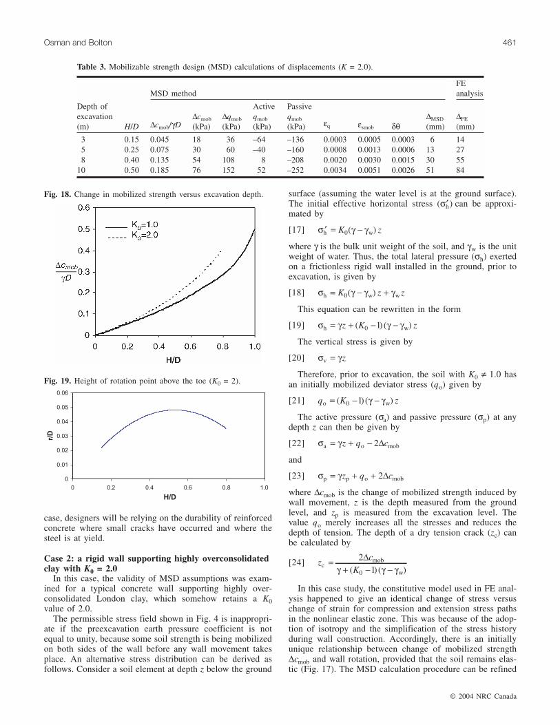
Fig. 18. Change in mobilized strength versus excavation depth.

Fig. 19. Height of rotation point above the toe (K0 = 2).

© 2004 NRC Canada

462 Can. Geotech. J. Vol. 41, 2004

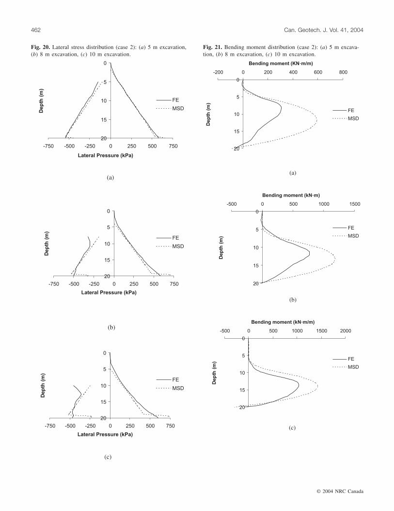
Fig. 20. Lateral stress distribution (case 2): (a) 5 m excavation,(b) 8 m excavation, (c) 10 m excavation.

Fig. 21. Bending moment distribution (case 2): (a) 5 m excava-tion, (b) 8 m excavation, (c) 10 m excavation.

to take into account the differences between stress–straincurves in the active and passive zones whether due to soilstress history or anisotropy as follows:(1) Select the allowable displacement for the retaining wall.(2) Find the corresponding mobilized strain applicable to all

deformation zones.(3) Determine the active and passive strengths mobilized

from compression and extension triaxial tests, respec-tively. In these tests the stress paths followed duringwall installation and during excavation of the soil infront of the wall should be taken into account (Powrie etal. 1998). The corresponding excavation depth can thenbe determined by solving the equilibrium equations.

Figure 18 provides a solution for the normalized changeof the mobilized strength (∆cmob/γD) in the two cases whereK0 = 2.0 and K0 = 1.0, for the particular condition γ/γw = 2,the initial water table at the ground surface, and assumingthat ∆cmob remains the same for both sides of the wall. TheMSD solution shows that the magnitude of the change inmobilized strength in the case of walls of deeper penetrationis not much affected by the value of K0. The effect of K0 onthe mobilized strength increases with the increase of excava-tion. At H/D = 0.4, the change in mobilized shear strength isabout 18% larger in the K0 = 2.0 case than in the K0 = 1.0case. The pivot point calculated on this assumption is about5% of the total wall height above the toe in the K0 = 2.0 case(Fig. 19).

Table 3 shows a comparison of the predicted displace-ments between FE and MSD for K0 = 2.0. In the MSD cal-culations the representative stress–strain curve of Fig. 17was used. Figure 20 compares the lateral stress distributions.The MSD bending moment predictions are shown in Fig. 21to be conservative with respect to FE analysis, but not exces-sively so. The new approach of allowing for an offset ininitial deviatoric stress due to K0 effects is shown to be suc-cessful.

Effects of wall flexibility and K0The impact of the various parameters that influence wall

movements in the short term was studied. The displacementsof the crest of the wall calculated by the MSD method(∆MSD) are normalized by the FE displacements (∆FE) andare related to wall flexibility for different in situ lateral earthpressure coefficients (K0), different shapes of soil stress–strain curve, and different excavation ratios, defined as theexcavated depth divided by the overall height of the wall.

The wall flexibility can be characterized by the non-dimensional group (R), which was introduced by Rowe(1955). R is defined as the relative soil–structure stiffnessand is given by

[25] RmH=

4

EI

© 2004 NRC Canada

Osman and Bolton 463

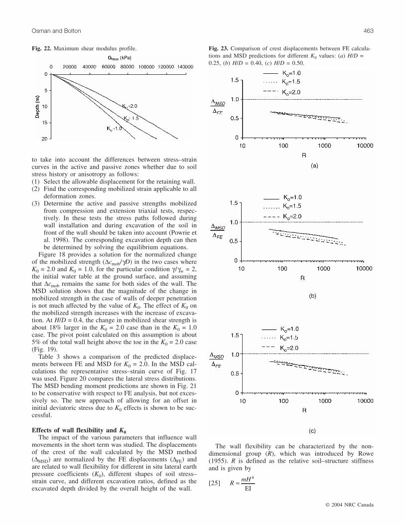
Fig. 22. Maximum shear modulus profile. Fig. 23. Comparison of crest displacements between FE calcula-tions and MSD predictions for different K0 values: (a) H/D =0.25, (b) H/D = 0.40, (c) H/D = 0.50.

where H is the height of the wall, and EI is the bending stiff-ness per unit width. The parameter m can be defined as therate of change of the shear modulus with depth (Powrie andLi 1991). In this case, it may be acceptable to calculate arepresentative m by fitting the best straight line through theorigin of the plot of the maximum shear modulus (Gmax) ver-sus depth (Fig. 22).

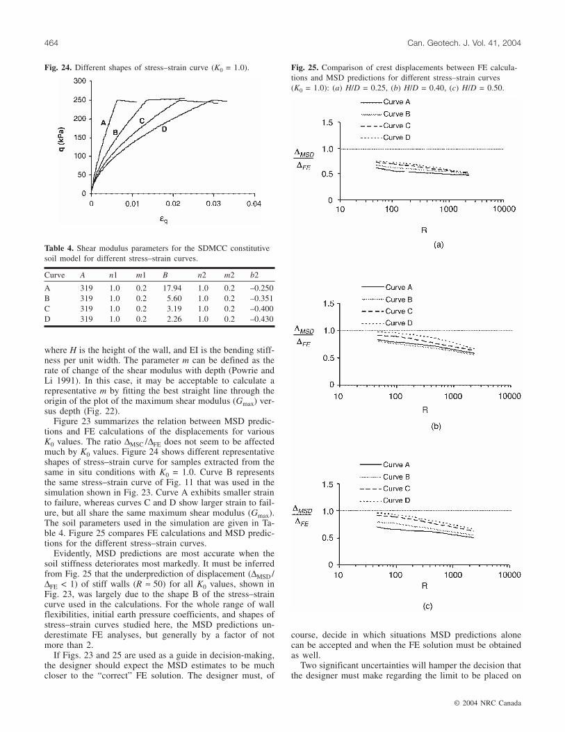
Figure 23 summarizes the relation between MSD predic-tions and FE calculations of the displacements for variousK0 values. The ratio ∆ ∆MSC FE/ does not seem to be affectedmuch by K0 values. Figure 24 shows different representativeshapes of stress–strain curve for samples extracted from thesame in situ conditions with K0 = 1.0. Curve B representsthe same stress–strain curve of Fig. 11 that was used in thesimulation shown in Fig. 23. Curve A exhibits smaller strainto failure, whereas curves C and D show larger strain to fail-ure, but all share the same maximum shear modulus (Gmax).The soil parameters used in the simulation are given in Ta-ble 4. Figure 25 compares FE calculations and MSD predic-tions for the different stress–strain curves.

Evidently, MSD predictions are most accurate when thesoil stiffness deteriorates most markedly. It must be inferredfrom Fig. 25 that the underprediction of displacement (∆MSD /∆FE < 1) of stiff walls (R ≈ 50) for all K0 values, shown inFig. 23, was largely due to the shape B of the stress–straincurve used in the calculations. For the whole range of wallflexibilities, initial earth pressure coefficients, and shapes ofstress–strain curves studied here, the MSD predictions un-derestimate FE analyses, but generally by a factor of notmore than 2.

If Figs. 23 and 25 are used as a guide in decision-making,the designer should expect the MSD estimates to be muchcloser to the “correct” FE solution. The designer must, of

course, decide in which situations MSD predictions alonecan be accepted and when the FE solution must be obtainedas well.

Two significant uncertainties will hamper the decision thatthe designer must make regarding the limit to be placed on

© 2004 NRC Canada

464 Can. Geotech. J. Vol. 41, 2004

Fig. 24. Different shapes of stress–strain curve (K0 = 1.0).

Curve A n1 m1 B n2 m2 b2

A 319 1.0 0.2 17.94 1.0 0.2 –0.250B 319 1.0 0.2 5.60 1.0 0.2 –0.351C 319 1.0 0.2 3.19 1.0 0.2 –0.400D 319 1.0 0.2 2.26 1.0 0.2 –0.430

Table 4. Shear modulus parameters for the SDMCC constitutivesoil model for different stress–strain curves.

Fig. 25. Comparison of crest displacements between FE calcula-tions and MSD predictions for different stress–strain curves(K0 = 1.0): (a) H/D = 0.25, (b) H/D = 0.40, (c) H/D = 0.50.

wall movement or soil strain. Designers should first realisethat criteria for limiting strains to prevent damage in differ-ent classes of structure are rather approximate (Burland andWroth 1974). The actual condition of the existing buildingor services that are partly located in the zone of influence ofa new excavation will also be open to doubt. These inevita-ble uncertainties may lead the designer to the conclusionthat even a factor 2 error in the MSD calculations can be tol-erated.

Conclusions

Serviceability and safety requirements should be based onthe fundamental understanding of the stress–strain behaviourof the soil. The design strength that limits the deformationsshould be selected according to the actual stress–strain datafrom each site, and not derived using arbitrary factors. Thepresent study relates to the undrained soil response to exca-vation behind a cantilever retaining wall.

A new application of plasticity theory that combines stati-cally admissible stress fields and kinematically admissibledeformation mechanisms with distributed plastic strains canprovide a unified solution for design problems. This applica-tion is different from the conventional applications of plas-ticity theory because it can approximately satisfy both safetyand serviceability requirements by predicting stresses anddisplacements under working conditions. Also, it providessimple hand calculations for nonlinear soil behaviour whichcan give reasonable results compared with those from com-plex finite element analyses.

Displacements in the MSD method are controlled by theaverage soil stiffness in the zone of deformation. Stress–strain data from an undisturbed soil sample taken at the mid-height of the retaining wall prior to excavation can be usedto deduce the average shear strength that can be mobilized atthe required shear strain in MSD calculations.

More generalized statically admissible stress fields werederived for the MSD method to incorporate the K0 effect.Although the MSD method overestimates the depth of ten-sion cracks developed in soils and ignores wall friction, itgives lateral stress distributions similar to those calculatedby FE analysis. Bending moments are very sensitive even tosmall changes in stress distribution, however, and care needsto be taken in selecting appropriate values.

Curves showing the variation in the ratios of crest defor-mations predicted by the MSD method compared with thosecalculated using FE analysis are plotted against Rowe’s rela-tive soil–structure stiffness for various in situ values of K0,various stress–strain curves, and various excavation ratios.These curves can be useful in the preliminary design ofretaining walls. They show that the MSD method under-predicts displacements, but generally by a factor smallerthan 2, which could be acceptable in many practical designsituations. Recalibration of MSD predictions based on thegiven curves could lead to even more accurate predictions.

The key advantage of the MSD method is that it gives thedesigners the opportunity to consider the sensitivity of a de-sign proposal to the nonlinear behaviour of a representativesoil element. It accentuates the importance of acquiring rea-sonably undisturbed samples and of testing them with an ap-

propriate degree of accuracy in the local measurement ofstrains (e.g., 0.01%). The extra step of actually performingFE analyses remains open, with the advantage that the engi-neer would then have an independent check on the answer tobe expected, within a factor of 2 on displacement and a fac-tor of 1.5 on bending moment.

It has been illustrated that a wall designed to resist MSDearth pressure cannot collapse if the wall is designed to beductile. If extra bending moments are induced due to exces-sive wall stiffness, plastic yielding will eliminate them as thewall displacement increases by a negligible amount.

Acknowledgements

The authors would like to thank Dr. Arul Britto for hisadvice and helpful comments. The authors are grateful toCambridge Commonwealth Trust and Overseas ResearchScheme for their provision of financial support to the firstauthor.

References

Atkinson, J.H., Richardson, D., and Stallebrass, S.E. 1990. Effectof recent stress history on the stiffness of overconsolidated soil.Géotechnique, 40(4): 531–540.

Bolton, M.D. 1993. Codes, standard and design guides. In Re-taining structures. Edited by C.R.I. Clayton. Thomas Telford,London, UK. pp. 387–402.

Bolton, M.D., and Powrie, W. 1987. The collapse of diaphramwalls retaining clay. Géotechnique, 37(3): 335–353.

Bolton, M.D., and Powrie, W. 1988. Behaviour of diaphram wallsin clay prior to collapse. Géotechnique, 38(2): 167–189.

Bolton, M.D., and Sun, H.W. 1991. Modelling of bridge abutmentson stiff clay. In Proceedings of the 10th European Conferenceon Soil Mechanics, Florence, Italy, 26–30 May 1991. A.A.Balkema, Rotterdam, The Netherlands. Vol. 1, pp. 51–55.

Bolton, M.D., Powrie, W., and Symons, I.F. 1989. The design ofstiff in-situ walls retaining overconsolidated clay, part 1. GroundEngineering, 22(8): 44–48.

Bolton, M.D., Powrie,W., and Symons, I.F. 1990a. The design ofstiff in-situ walls retaining overconsolidated clay, part 1, shortterm behaviour. Ground Engineering, 23(1): 34–39.

Bolton, M.D., Powrie, W., and Symons, I.F. 1990b. The design ofstiff in-situ walls retaining overconsolidated clay, part II, longterm behaviour. Ground Engineering, 23(2): 22–28.

Bolton, M.D., Dasari, G.R., and Britto, A.M. 1994. Putting smallstrain non-linearity into Modified Cam Clay model. In Proceed-ings of the 8th International Conference on Computer Methodsand Advances in Geomechanics (IACMAG), Morgantown, W.Va., 22–28 May 1994. Edited by J. Siriwardane and M.M.Zaman. A.A. Balkema, Rotterdam, The Netherlands. pp. 537–542.

British Standards Institution. 1994. Code of practice for earth re-taining structures. BS 8002. British Standards Institution, Lon-don, UK.

Burland, J.B., and Wroth, C.P. 1974. Allowable and differentialsettlements of structures, including damage and soil–structureinteraction. In Settlement of Structures, Proceedings of the Con-ference of the British Geotechnical Society, Cambridge. PentechPress, London, UK. pp. 611–764.

© 2004 NRC Canada

Osman and Bolton 465

© 2004 NRC Canada

466 Can. Geotech. J. Vol. 41, 2004

Burland, J.B., Potts, D.M., and Walsh, N.M. 1981. Overall stabilityof free and propped embedded cantilever retaining walls.Ground Engineering, 14(5): 28–32, 35–37.

Carder, D.R., and Symons, I.F. 1989. Long-term performance of anembedded cantilever retaining wall in stiff clay. Géotechnique,39(1): 55–75.

Dasari, G.R. 1996. Modelling the variation of soil stiffness duringsequential construction. Ph.D. dissertation, Cambridge Univer-sity, Cambridge, UK.

Dasari, G.R., and Britto, A.M. 1995. Strain-dependent ModifiedCam Clay model. Technical Report CUED-SOILS/TR276, Cam-bridge University Engineering Department, Cambridge Univer-sity, Cambridge, UK.

De Moor, E.K. 1994. Analysis of bored pile/diaphragm wall instal-lation effects. Géotechnique, 44(2): 341–347.

ECS. 1997. Eurocode EC7: geotechnical design. European Com-mittee for Standardization (ECS), Brussels, Belgium.

Garrett, C., and Barnes, S.J. 1984. Design and performance of theDunton Green retaining wall. Géotechnique, 34(4): 533–548.

Hubbard, H.W., Potts, D.M., Miller, D., and Burland, J.B. 1984.Design of the retaining walls for the M25 cut and cover tunnelat Bell Common. Géotechnique, 34(4): 495–512.

Jardine, R.J., Symes, M.J., and Burland, J.B. 1984. The measure-ment of soil stiffness in the triaxial apparatus. Géotechnique,34(3): 323–340.

Long, M. 2001. Database for retaining wall and ground movementsdue to deep excavations. Journal of Geotechnical and Geo-environmental Engineering, ASCE, 127(3): 203–224.

Masing, G. 1926. Eigenspannungen und Verfestigung beimMessing. In Proceedings of the 2nd International Congress ofApplied Mechanics, Zurich, Switzerland. pp. 332–335.

Milligan, G.W.E., and Bransby, P.L. 1976. Combined active andpassive rotational failure of a retaining wall in sand. Géo-technique, 26(3): 473–494.

Osman, A.S. 2002. Mobilizable soil strength for geotechnical de-sign of retaining walls. M.Phil. dissertation, Department of En-gineering, Cambridge University, Cambridge, UK.

Padfield, C.J., and Mair, R.J. 1984. Design of retaining walls em-

bedded in stiff clay. Construction Industry Research and Infor-mation Association, CIRIA Report R104.

Potts, D.M., and Fourie, A.B. 1985. The effect of wall stiffness onthe behaviour of a propped retaining wall. Géotechnique, 35(3):347–352.

Powrie, W. 1985. Discussion on performance of propped and canti-levered rigid walls. Géotechnique, 35(4): 546–548.

Powrie, W. 1996. Limit equilibrium analysis of embedded retainingwalls. Géotechnique, 46(4): 709–723.

Powrie, W., and Li, E.S.F. 1991. Finite element analyses of an insitu wall propped at formation level. Géotechnique, 41(4): 499–514.

Powrie, W., Pantelidou, H., and Stallebrass, S.E. 1998. Soil stiff-ness in stress paths relevant to diaphragm walls in clay. Géo-technique, 48(4): 483–494.

Puller, M., and Lee, T. 1996. Comparison between the designmethods for earth retaining structures recommended by BS8002:1994 and previously used methods. Proceedings of the In-stitution of Civil Engineers, Geotechnical Engineering, 119(1):29–34.

Roscoe, K.H., and Burland, J.B. 1968. On the generalized stress–strain behaviour of wet clay. In Engineering plasticity. Edited byJ. Heyman and F.A. Leckie. Cambridge University Press, Cam-bridge, UK. pp. 535–609.

Rowe, P.W. 1955. Sheet pile walls encastre at the anchorage. Pro-ceedings of the Institution of Civil Engineers, London, Part 1,Vol. 4.

Simpson, B., and Driscoll, R. 1998. Eurocode 7: a commentary.Construction Research Communications, Watford, UK.

Symons, I.F. 1983. Assessing the stability of a propped, in situretaining wall in overconsolidated clay. Proceedings of the Insti-tution of Civil Engineers, Part 2: Research and Theory, 75: 617–633.

Symons, I.F., and Carder, D.R. 1992. Field measurement on em-bedded retaining walls. Géotechnique, 42(1): 117–126.

Tedd, P., Chard, B.M., Charles, J.A., and Symons, I.F. 1984. Be-haviour of a propped embedded retaining wall in stiff clay atBell Common Tunnel. Géotechnique, 34(4): 513–532.