Antialiasing CSE167: Computer Graphics Instructor: Steve Rotenberg UCSD, Fall 2006.
date post
21-Dec-2015Category
view
222download
2
#14: Ray Tracing II &Antialiasing
CSE167: Computer GraphicsInstructor: Ronen Barzel
UCSD, Winter 2006
2
Outline for today
Speeding up Ray Tracing Antialiasing Stochastic Ray Tracing
3
Where we are now
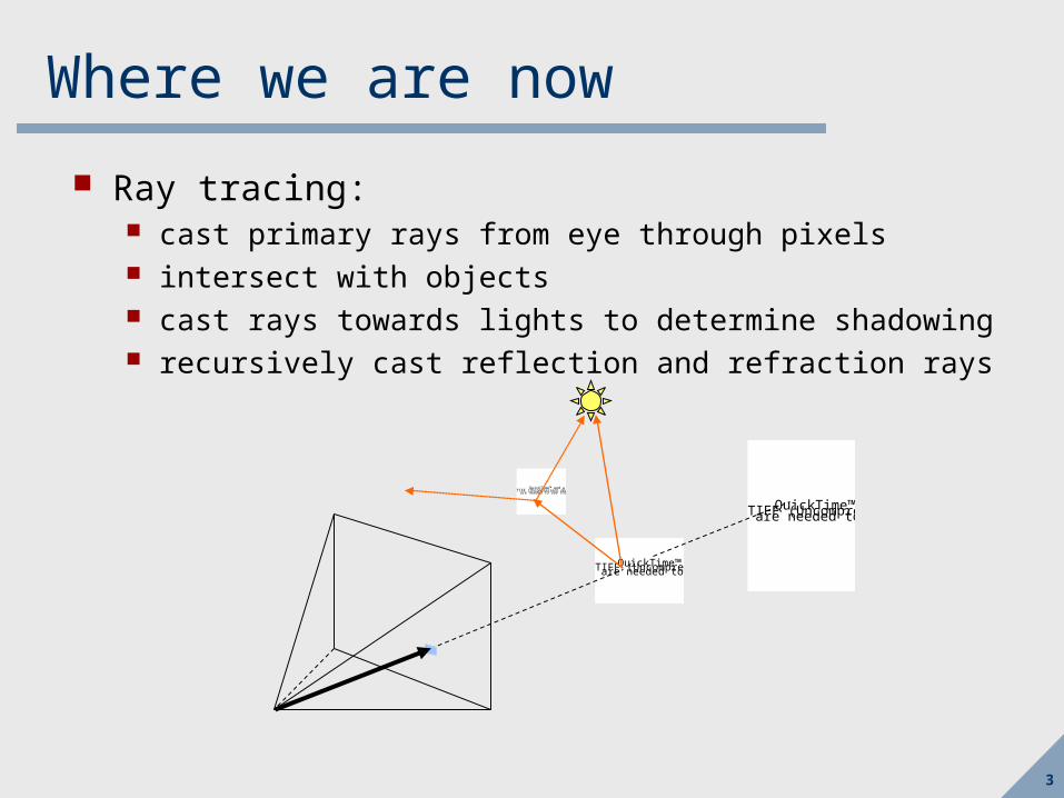
Ray tracing: cast primary rays from eye through pixels intersect with objects cast rays towards lights to determine shadowing recursively cast reflection and refraction rays
QuickTime™ and aTIFF (Uncompressed) decompressorare needed to see this picture.
QuickTime™ and aTIFF (Uncompressed) decompressorare needed to see this picture.
QuickTime™ and aTIFF (Uncompressed) decompressor
are needed to see this picture.
4
Need for acceleration structures
Lots of rays: Scenes can contain millions or billions of primitives Ray tracers need to trace millions of rays This means zillions of potential ray-object intersections
Infeasible to test every object for intersection Just looping through all objects*rays would take days Not even counting time to do the intersection testing or
illumination Acceleration structures
Major goal: minimize number of intersection tests• Tests that would return false (no intersection)• Tests that would return an intersection that’s not closest to origin
Core approach: Hierarchical subdivision of space• Can reduce O(N) tests to O(log(N)) tests
(Other acceleration techniques too… beam tracing, cone tracing, photon maps, …)
5
Bounding Volume Hierarchies
Enclose objects with hierarchy of simple shapes Same idea as for frustum culling Test ray against outermost bounding volume
• If ray misses bounding volume, can reject entire object
• If ray intersects volume, recurse to child bounding volumes
• When reaching the leaves of the hierarchy, intersect with primitives
Can keep track of current nearest intersection along ray• If bounding volume is farther away that, no need to test intersection
6
Culling complex objects or groups
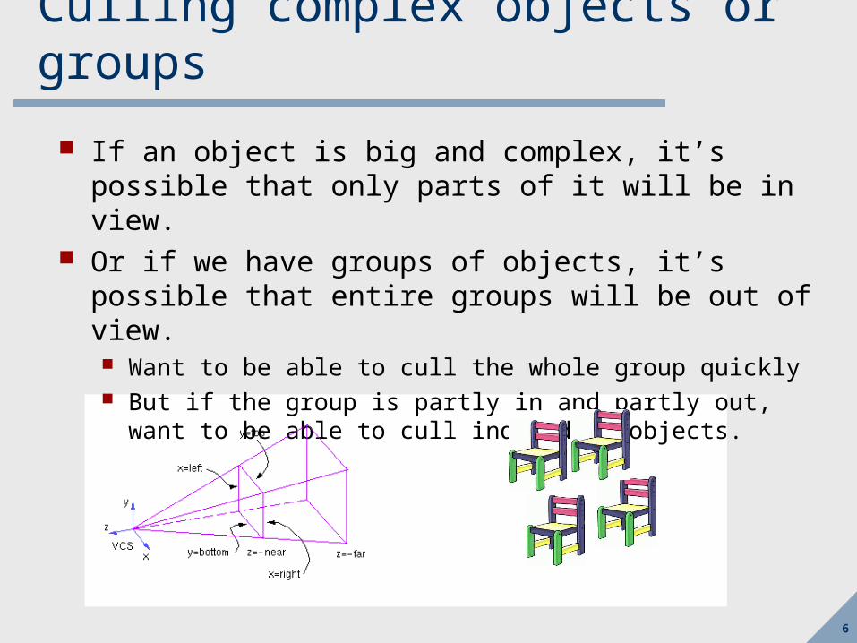
If an object is big and complex, it’s possible that only parts of it will be in view.
Or if we have groups of objects, it’s possible that entire groups will be out of view. Want to be able to cull the whole group quickly But if the group is partly in and partly out, want to be able to cull individual objects.
7
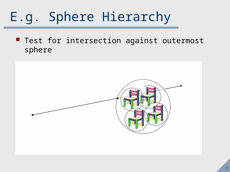
E.g. Sphere Hierarchy
Test for intersection against outermost sphere
8
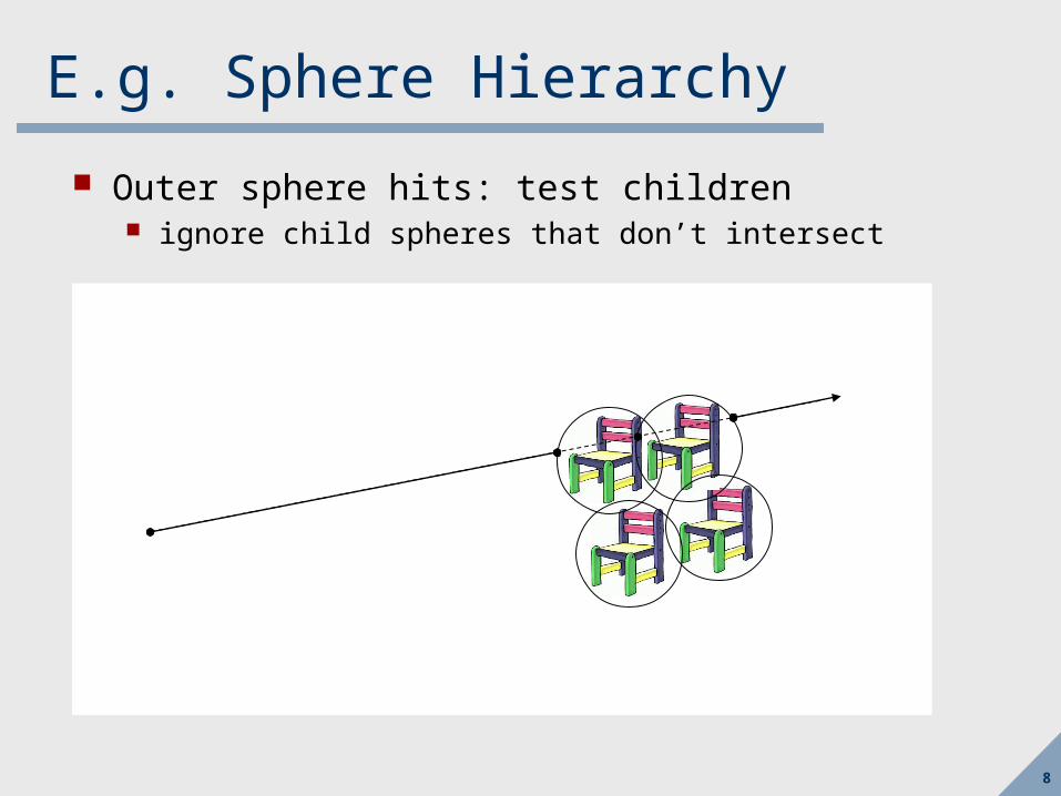
E.g. Sphere Hierarchy
Outer sphere hits: test children ignore child spheres that don’t intersect
9
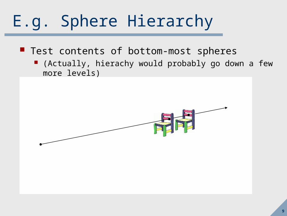
E.g. Sphere Hierarchy
Test contents of bottom-most spheres (Actually, hierachy would probably go down a few more levels)
10
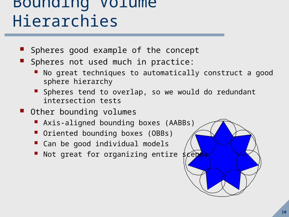
Bounding Volume Hierarchies
Spheres good example of the concept Spheres not used much in practice:
No great techniques to automatically construct a good sphere hierarchy
Spheres tend to overlap, so we would do redundant intersection tests
Other bounding volumes Axis-aligned bounding boxes (AABBs) Oriented bounding boxes (OBBs) Can be good individual models Not great for organizing entire scenes

11
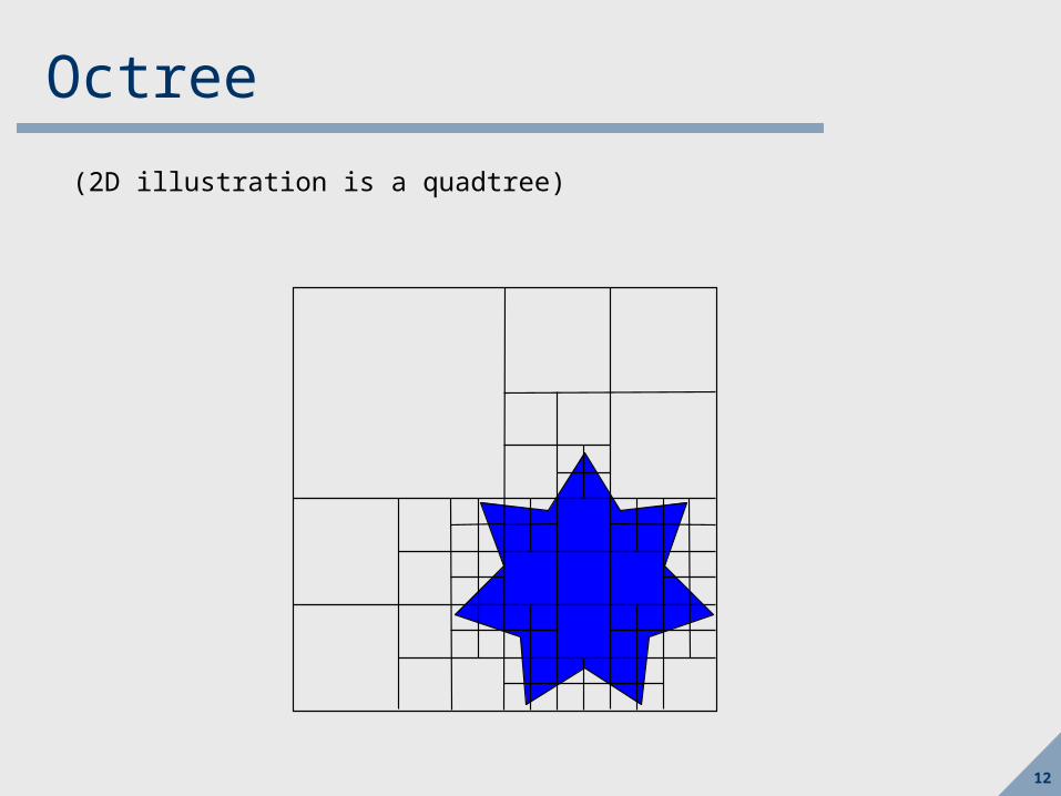
Octrees Start by placing a cube around the entire scene If the cube contains “too many” primitives (say,
10) split equally into 8 nested cubes recursively test and possibly subdivide each of those
cubes More regular structure than the sphere tree Provides a clear rule for subdivision and no
overlap between cells This makes it a better choice than sphere usually But still not ideal; lots of empty cubes
12
Octree
(2D illustration is a quadtree)
13
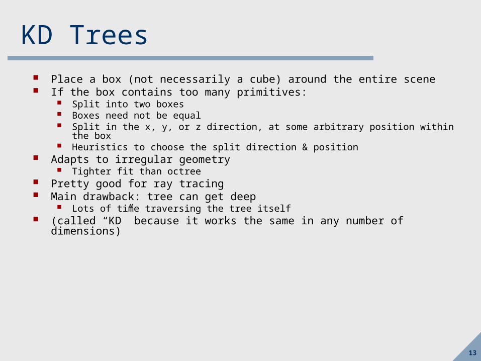
KD Trees Place a box (not necessarily a cube) around the entire scene If the box contains too many primitives:
Split into two boxes Boxes need not be equal Split in the x, y, or z direction, at some arbitrary position within
the box Heuristics to choose the split direction & position
Adapts to irregular geometry Tighter fit than octree
Pretty good for ray tracing Main drawback: tree can get deep
Lots of time traversing the tree itself (called “KD” because it works the same in any number of
dimensions)
14
KD Tree
15
BSP Trees
Binary Space Partitioning (BSP) tree Start with all of space If there are too many objects, split into two
subspaces: choose a plane to divide the space in two the plane can be placed anywhere and oriented any
direction heuristics to choose a good plane recurse to children
Similar to KD tree: recursively splits space into two (unequal) parts Potential to more tightly bound objects Harder to choose splitting plane Harder to work with arbitrary-shaped regions
In practice, BSP trees tend to perform well for ray tracing

16
BSP Tree
17
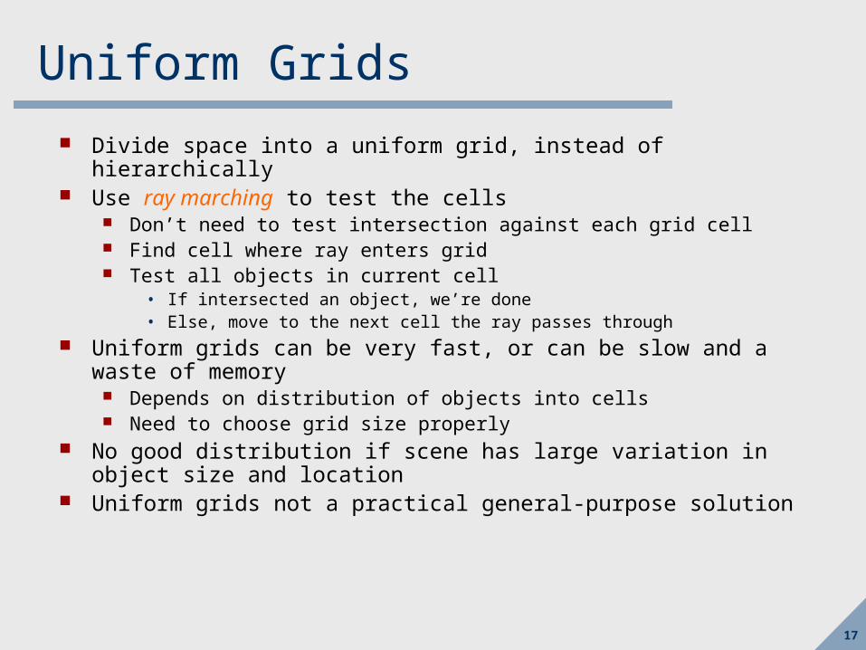
Uniform Grids Divide space into a uniform grid, instead of
hierarchically Use ray marching to test the cells
Don’t need to test intersection against each grid cell Find cell where ray enters grid Test all objects in current cell
• If intersected an object, we’re done• Else, move to the next cell the ray passes through
Uniform grids can be very fast, or can be slow and a waste of memory
Depends on distribution of objects into cells Need to choose grid size properly
No good distribution if scene has large variation in object size and location
Uniform grids not a practical general-purpose solution
18
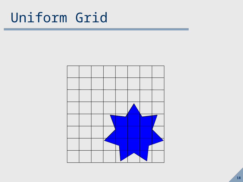
Uniform Grid

19
Ray Marching
1 2 3
4 5 6
20
Hierarchical Grids
Start with a uniform grid If any cell has too many primitives
subdivide that cell into a grid subgrid can have any number of cells recurse if needed
(Octree: a hierarchical grid limited to 2x2x2 subdivision
Hierarchical grids can perform very well
21
Acceleration Structures Ray tracers always use acceleration structures to make the
algorithm feasible No one “best” structure Ongoing research into new structures and new ways of using
existing structures Considerations include:
Memory overhead of data structure Preprocessing time to construct data structure Ability to optimize well, given machine architecture For animation: Ability to update data structure as objects move
22
Outline for today
Speeding up Ray Tracing Antialiasing Stochastic Ray Tracing
23
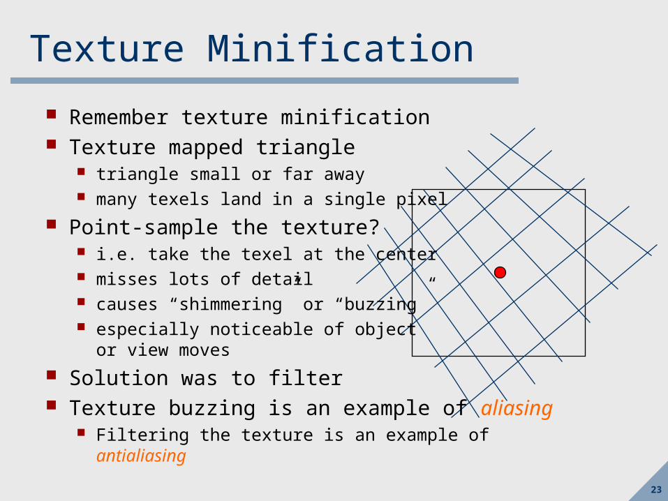
Texture Minification
Remember texture minification Texture mapped triangle
triangle small or far away many texels land in a single pixel
Point-sample the texture? i.e. take the texel at the center misses lots of detail causes “shimmering” or “buzzing” especially noticeable of object or view moves
Solution was to filter Texture buzzing is an example of aliasing Filtering the texture is an example of antialiasing
24
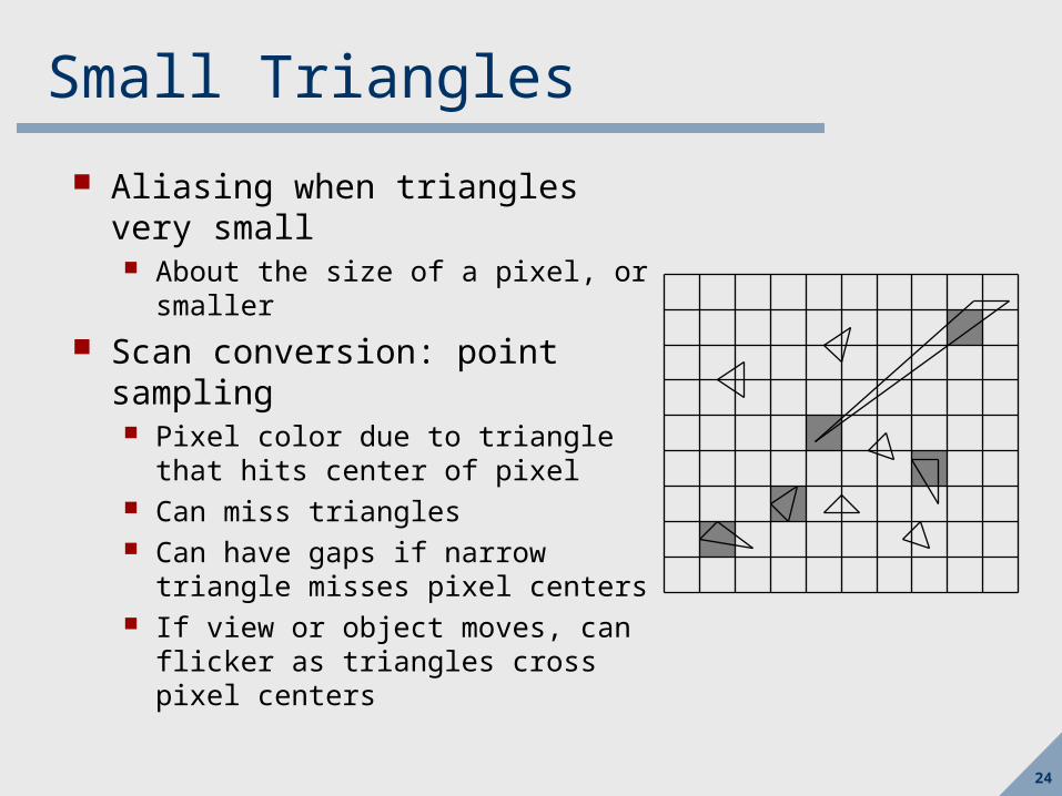
Small Triangles
Aliasing when triangles very small About the size of a pixel, or smaller
Scan conversion: point sampling Pixel color due to triangle that hits center of pixel
Can miss triangles Can have gaps if narrow triangle misses pixel centers
If view or object moves, can flicker as triangles cross pixel centers
25
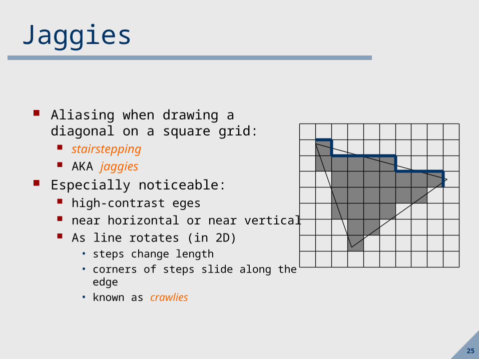
Jaggies
Aliasing when drawing a diagonal on a square grid: stairstepping AKA jaggies
Especially noticeable: high-contrast eges near horizontal or near vertical As line rotates (in 2D)
• steps change length• corners of steps slide along the edge
• known as crawlies
26
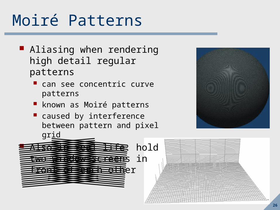
Moiré Patterns
Aliasing when rendering high detail regular patterns can see concentric curve patterns
known as Moiré patterns caused by interference between pattern and pixel grid
Also in real life: hold two window screens in front of each other
27
Strobing Consider 30 frame-per-second animation of a spinning propeller If the propeller is spinning at 1 rotation per second
each frame shows propeller rotated 12 degrees more than previous looks OK
If the propeller is spinning at 30 rotations per second each image shows propeller rotated 360 degrees i.e. in same place as previous frame i.e. propeller appears to stand still
If the propeller is spinning at 31 rotations per second: will appear to rotate slowly forwads 29 rotations per second: will appear to rotate slowly backwards
Example of strobing problems temporal aliasing caused by point-sampling the motion in time
28
Aliasing These examples cover a wide range of problems…
… but they all result from essentially the same thing
The image we are making is trying to represent a continuous signal The “true” image color is a function that varies with continuous X & Y
(and time) values For digital computation, our standard approach is to:
sample the original signal at discrete points (pixel centers or texels or wherever)
Use the samples to reconstruct a new signal, that we present to the audience
Want the audience to perceive the new signal the same as the original would be
Unfortunately, the sampling/reconstruction process causes some data to be misrepresented
Hence the term alias: some part of the signal masquerading as something else
Often refer to instances of problems as artifacts or aliasing artifacts
Antialiasing: trying to avoid aliasing problems. Three basic approaches:
Modify the original data so that it won’t have properties that cause aliasing
Use more sophisticated sampling/reconstruction techniques Clean up the artifacts after-the-fact

29
Signal Analysis Signal Analysis: the field that studies these problems in pure
form Applies also to digital audio, electrical engineering, radio, … Artifacts are different, but the theory is the same
Includes a variety of mathematical and engineering methods for working with signals:
Fourier analysis, sampling theory, filter, digital signal processing (DSP), … Kinds of signals:
electrical: a voltage changing over time. 1D signal: e = f(t) audio: sound pressure changing over time. 1D signal: a = f(t) computer graphics image: color changing over space. 2D signal: c=f(x,y) computer graphics animation: color changing over space & time. 3D signal:
c=f(x,y,t) Examples and concepts typically shown for scalar 1D signal
but they extend to more dimensions for the signal parameters but they extend to more dimensions for the signal value
A signal:
30
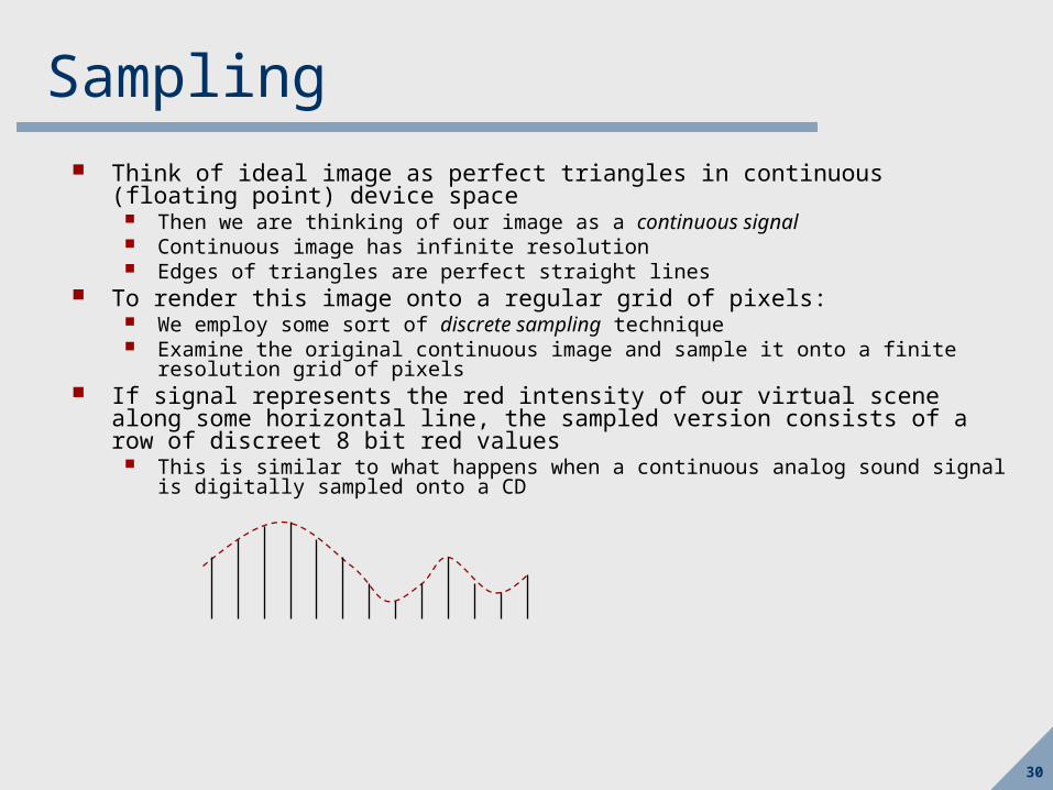
Sampling Think of ideal image as perfect triangles in continuous
(floating point) device space Then we are thinking of our image as a continuous signal Continuous image has infinite resolution Edges of triangles are perfect straight lines
To render this image onto a regular grid of pixels: We employ some sort of discrete sampling technique Examine the original continuous image and sample it onto a finite
resolution grid of pixels If signal represents the red intensity of our virtual scene
along some horizontal line, the sampled version consists of a row of discreet 8 bit red values
This is similar to what happens when a continuous analog sound signal is digitally sampled onto a CD
31
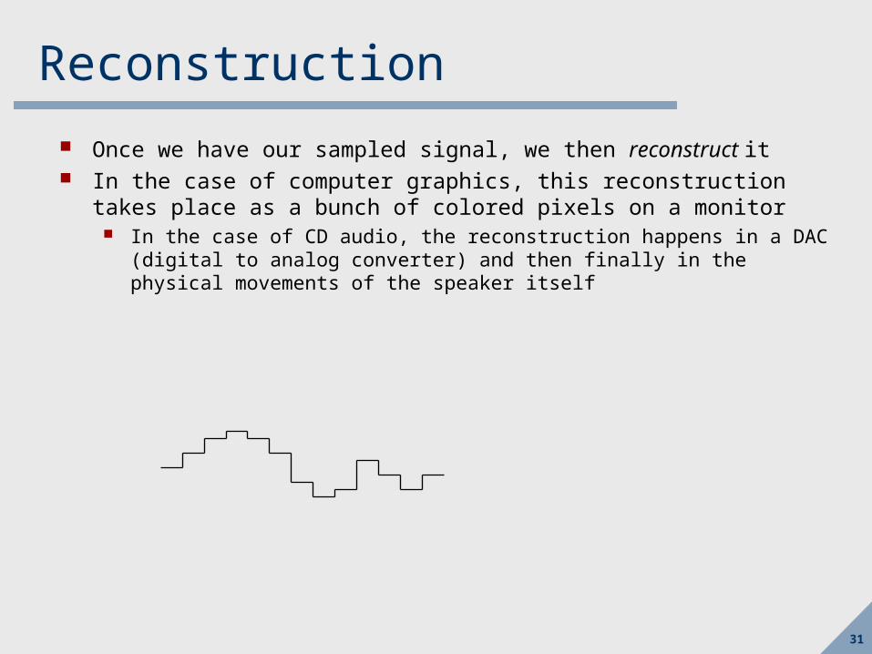
Reconstruction
Once we have our sampled signal, we then reconstruct it In the case of computer graphics, this reconstruction
takes place as a bunch of colored pixels on a monitor In the case of CD audio, the reconstruction happens in a DAC
(digital to analog converter) and then finally in the physical movements of the speaker itself
32
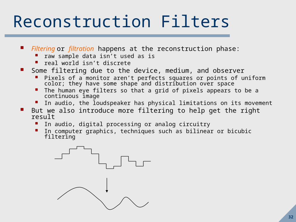
Reconstruction Filters Filtering or filtration happens at the reconstruction phase:
raw sample data isn’t used as is real world isn’t discrete
Some filtering due to the device, medium, and observer Pixels of a monitor aren’t perfects squares or points of uniform
color; they have some shape and distribution over space The human eye filters so that a grid of pixels appears to be a
continuous image In audio, the loudspeaker has physical limitations on its movement
But we also introduce more filtering to help get the right result
In audio, digital processing or analog circuitry In computer graphics, techniques such as bilinear or bicubic
filtering
33
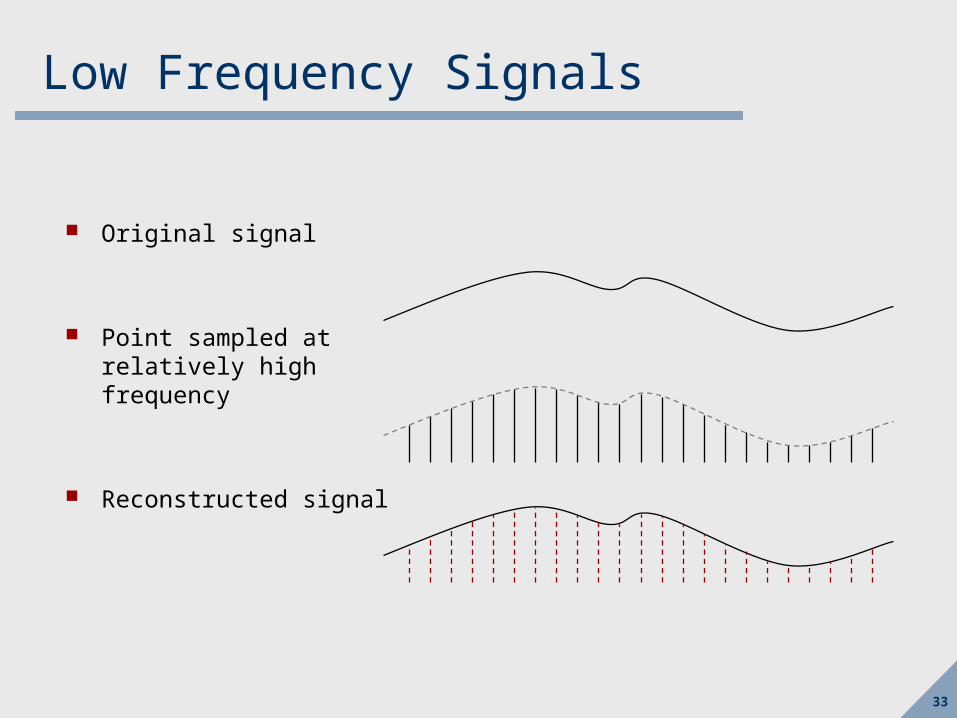
Low Frequency Signals
Original signal
Point sampled at relatively high frequency
Reconstructed signal
34
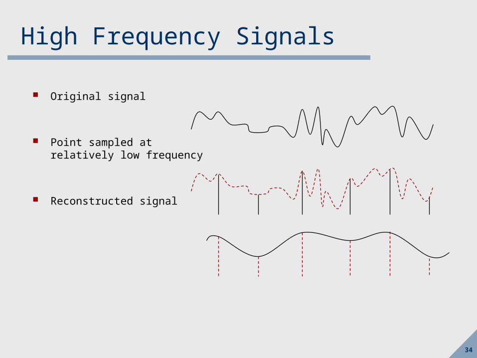
High Frequency Signals
Original signal
Point sampled at relatively low frequency
Reconstructed signal
35
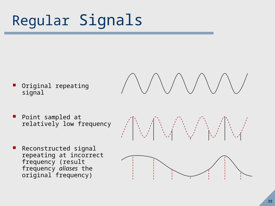
Regular Signals
Original repeating signal
Point sampled at relatively low frequency
Reconstructed signal repeating at incorrect frequency (result frequency aliases the original frequency)
36
Nyquist Limit
Any signal can be considered as a sum of signals with varying frequencies
That’s what an equalizer or spectrum display on an audio device shows
In order to correctly reconstruct a signal whose highest frequency is x:
sampling rate must have frequency at least 2x This is known as the Sampling Theorem
• AKA Nyquist Sampling Theorem, AKA Nyquist-Shannon Sampling Theorem
The 2x sampling frequency is known as the Nyquist frequency or Nyquist limit
Frequencies below the Nyquist limit come through OK Frequencies above the Nyquist limit come through as
lower-frequency aliases, mixed in with the data
37
Nyquist Limit
In images, having high (spatial) frequencies means: having lots of detail having sharp edges
Basic way to avoid aliasing: choose sampling rate higher than Nyquist limit
This assumes we are doing idealized sampling and reconstruction
In practice, better to sample at least 4x But in practice, we don’t always know the highest frequency In fact, we might not have an upper limit!
• E.g. checkerboard pattern receding to the horizon in perspective• Spatial frequency is infinite• Must use antialiasing techniques
38
Aliasing Problems, summary Shimmering / Buzzing:
Rapid pixel color changes (flickering) caused by high detail textures or high detail geometry. Ultimately due to point sampling of high frequency color changes at low frequency pixel intervals
Stairstepping / Jaggies:Noticeable stairstep edges on high contrast edges that are nearly horizontal or vertical. Due to point sampling of effectively infinite frequency color changes (step gradient at edge of triangle)
Moiré patterns:Strange swimming patterns that show up on regular patterns. Due to sampling of regular patterns on a regular pixel grid
Strobing:Incorrect or discontinuous motion in fast moving animated objects. Due to low frequency sampling of regular motion in regular time intervals. (temporal aliasing)
39
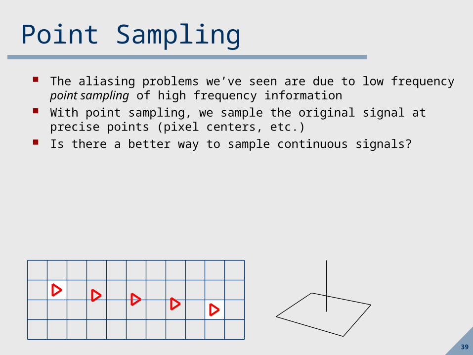
Point Sampling
The aliasing problems we’ve seen are due to low frequency point sampling of high frequency information
With point sampling, we sample the original signal at precise points (pixel centers, etc.)
Is there a better way to sample continuous signals?
40
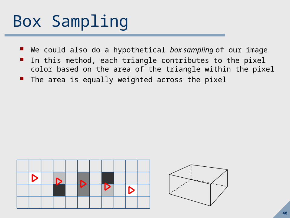
Box Sampling
We could also do a hypothetical box sampling of our image In this method, each triangle contributes to the pixel
color based on the area of the triangle within the pixel The area is equally weighted across the pixel
41
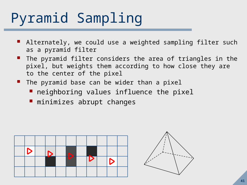
Pyramid Sampling
Alternately, we could use a weighted sampling filter such as a pyramid filter
The pyramid filter considers the area of triangles in the pixel, but weights them according to how close they are to the center of the pixel
The pyramid base can be wider than a pixel neighboring values influence the pixel minimizes abrupt changes
42
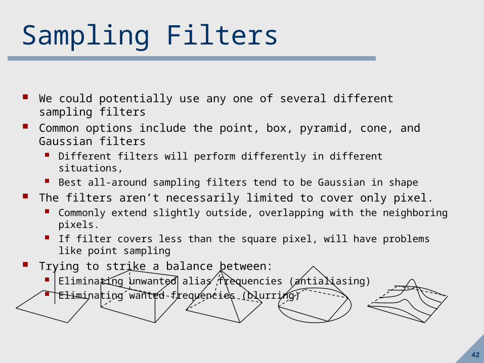
Sampling Filters
We could potentially use any one of several different sampling filters
Common options include the point, box, pyramid, cone, and Gaussian filters
Different filters will perform differently in different situations,
Best all-around sampling filters tend to be Gaussian in shape The filters aren’t necessarily limited to cover only pixel.
Commonly extend slightly outside, overlapping with the neighboring pixels.
If filter covers less than the square pixel, will have problems like point sampling
Trying to strike a balance between: Eliminating unwanted alias frequencies (antialiasing) Eliminating wanted frequencies (blurring)
43
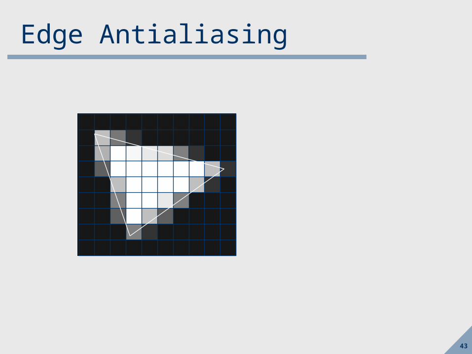
Edge Antialiasing
44
Pixel Coverage
Various antialiasing algorithms exist to color the pixel based on the exact area of the of the pixel that a triangle covers.
But, without storing a lot of additional information per pixel, very hard (or impossible) to properly handle case of several triangle edges in a single pixel
Impractical to make a coverage-based scheme compatible with z-buffering
Can do better if triangles are sorted back to front
Coverage approaches not generally used in practice for rendering
Still apply to things such as font filtering
45
Supersampling A more popular method (although less elegant) is
supersampling: Point sample the pixel at several locations Combine the results into the final pixel color
By sampling more times per pixel: Raises the sampling rate Raises the frequencies we can capture
Commonly use 16 or more samples per pixel Requires frame buffer and z-buffer to be 16 times as large Requires potentially 16 times as much work to generate image
A brute-force approach But straightforward to implement Very powerful
46
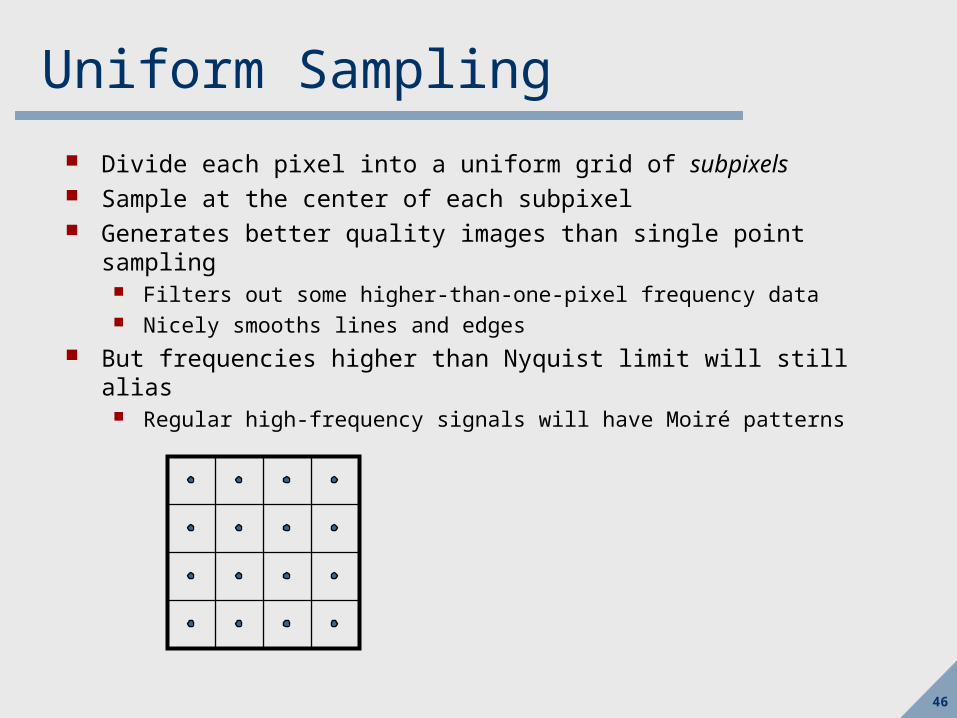
Uniform Sampling
Divide each pixel into a uniform grid of subpixels Sample at the center of each subpixel Generates better quality images than single point
sampling Filters out some higher-than-one-pixel frequency data Nicely smooths lines and edges
But frequencies higher than Nyquist limit will still alias
Regular high-frequency signals will have Moiré patterns
47
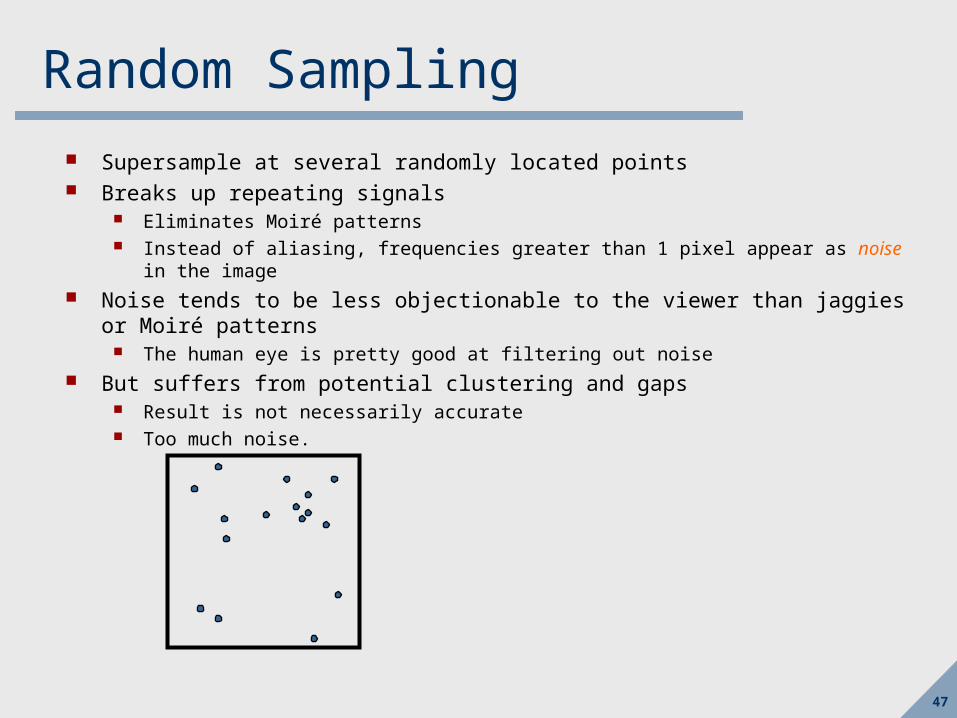
Random Sampling Supersample at several randomly located points Breaks up repeating signals
Eliminates Moiré patterns Instead of aliasing, frequencies greater than 1 pixel appear as noise
in the image Noise tends to be less objectionable to the viewer than jaggies
or Moiré patterns The human eye is pretty good at filtering out noise
But suffers from potential clustering and gaps Result is not necessarily accurate Too much noise.
48
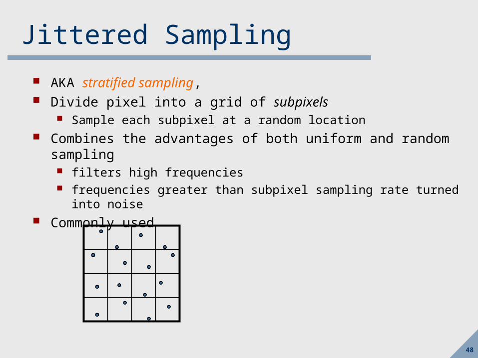
Jittered Sampling
AKA stratified sampling, Divide pixel into a grid of subpixels
Sample each subpixel at a random location Combines the advantages of both uniform and random
sampling filters high frequencies frequencies greater than subpixel sampling rate turned
into noise Commonly used
49
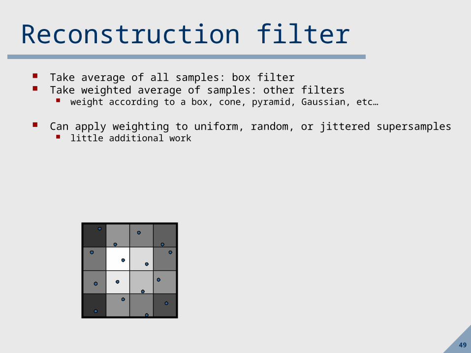
Reconstruction filter Take average of all samples: box filter Take weighted average of samples: other filters
weight according to a box, cone, pyramid, Gaussian, etc…
Can apply weighting to uniform, random, or jittered supersamples little additional work
50
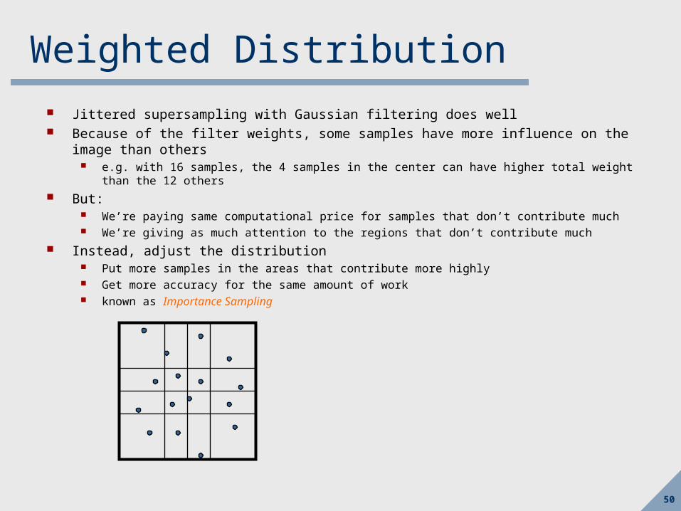
Weighted Distribution Jittered supersampling with Gaussian filtering does well Because of the filter weights, some samples have more influence on the
image than others e.g. with 16 samples, the 4 samples in the center can have higher total weight
than the 12 others But:
We’re paying same computational price for samples that don’t contribute much We’re giving as much attention to the regions that don’t contribute much
Instead, adjust the distribution Put more samples in the areas that contribute more highly Get more accuracy for the same amount of work known as Importance Sampling
51
Adaptive Sampling More sophisticated option is to perform adaptive
sampling Start with a small number of samples Analyze their statistical variation
It the colors are all similar, we accept that we have an accurate sampling
If the colors have a large variation, take more samples
continue until statistical error is within acceptable tolerance
Varying amount of work per pixel Concentrates work where the image is “hard”
Tricky to add samples while keeping good distribution But possible! Used in practice, especially in research renderers
52
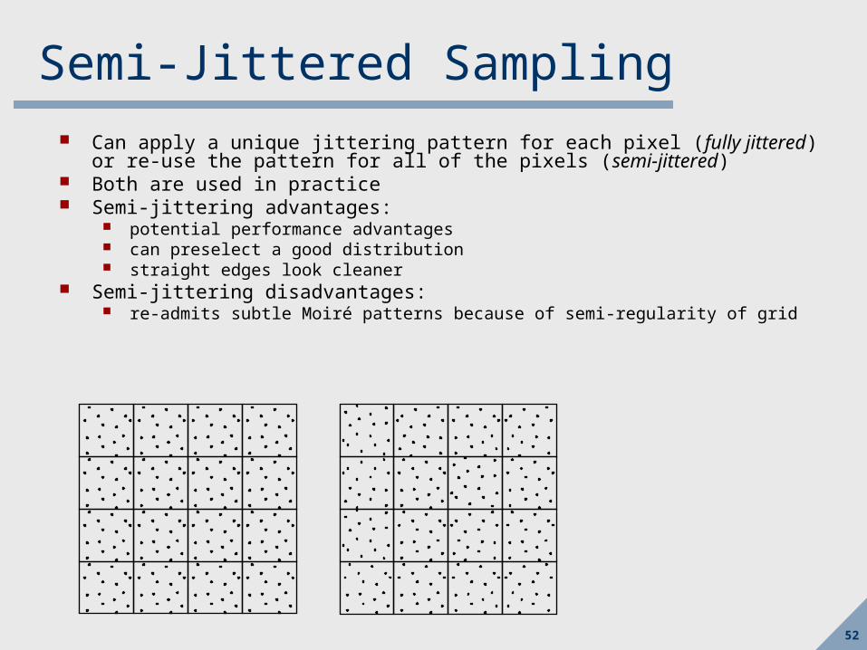
Semi-Jittered Sampling Can apply a unique jittering pattern for each pixel (fully
jittered)or re-use the pattern for all of the pixels (semi-jittered)
Both are used in practice Semi-jittering advantages:
potential performance advantages can preselect a good distribution straight edges look cleaner
Semi-jittering disadvantages: re-admits subtle Moiré patterns because of semi-regularity of grid
53
Mipmapping & Pixel Antialiasing
Mipmapping and other texture filtering techniques reduce texture aliasing problems
Combine mipmapping with pixel supersampling Choose mipmaps based on subpixel size Gets better edge-on behavior than mipmapping alone
But it’s expensive to compute shading at every supersample Hybrid approach:
Assume that mipmapping and filters in procedural shaders minimize aliasing at pixel scale
Compute only a single shading sample per pixel Still supersample the scan-conversion and z-buffer
Gives edge antialiasing of supersampling and texture filtering of mipmapping
Doesn’t require cost of full supersampling GPU hardware often does this:
Requires increase framebuffer/z-buffer memory But doesn’t slow down performance much Works pretty well
54
Motion Blur Looks cool in static images Improves perceived quality of
animation Details depend on display technology
(film vs CRT vs LCD vs. …) Generally speaking: the eye
normally blurs moving objects Animation is sequence of still
frames Sequence of unblurred still frames
look strangely unnatural• E.g. old Sinbad movies with stop-
motion monsters If objects in each frame are blurred
in the direction of motion, easier for brain to reconstruct continuous object.• In Dragonslayer (1981), go-motion
monster was introduced• Model moved with camera shutter open. • Noticeably better quality, even if
most people didn’t know why
• In CG special effects, motion blur always computed
QuickTime™ and aTIFF (Uncompressed) decompressor
are needed to see this picture.
55
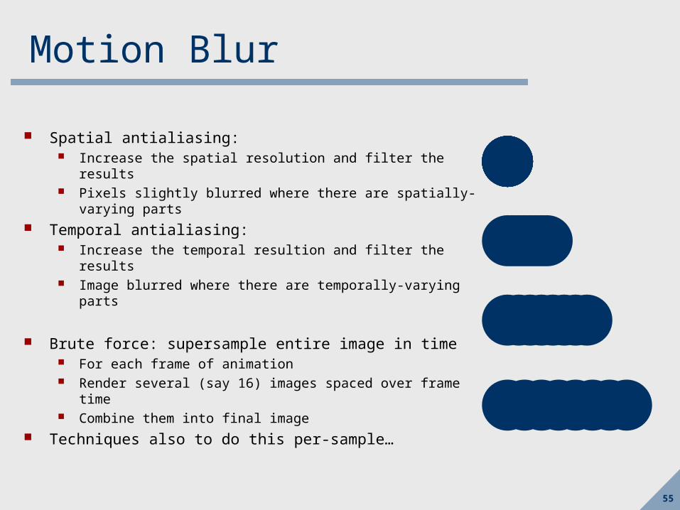
Motion Blur
Spatial antialiasing: Increase the spatial resolution and filter the
results Pixels slightly blurred where there are spatially-
varying parts Temporal antialiasing:
Increase the temporal resultion and filter the results
Image blurred where there are temporally-varying parts
Brute force: supersample entire image in time For each frame of animation Render several (say 16) images spaced over frame
time Combine them into final image
Techniques also to do this per-sample…
56
Outline for today
Speeding up Ray Tracing Antialiasing Stochastic Ray Tracing

57
Stochastic Ray Tracing
Introduced in 1984 (Cook, Porter, Carpenter) AKA distributed ray tracing AKA distribution ray
tracing (originally called “distributed”, but now that refers
to parallel processing)
Technique for achieving various fancy effects: Antialiasing Motion Blur Soft Shadows Area Lights Blurry Reflections Camera Focus/Depth-of-field …
The basic idea is to shoot more rays with values having an appropriate random distribution i.e. stochastically
58
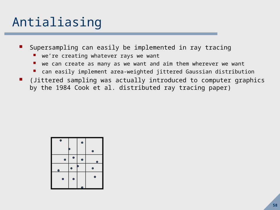
Antialiasing
Supersampling can easily be implemented in ray tracing we’re creating whatever rays we want we can create as many as we want and aim them wherever we want can easily implement area-weighted jittered Gaussian distribution
(Jittered sampling was actually introduced to computer graphics by the 1984 Cook et al. distributed ray tracing paper)
59
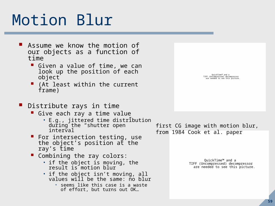
Motion Blur Assume we know the motion of
our objects as a function of time Given a value of time, we can
look up the position of each object
(At least within the current frame)
Distribute rays in time Give each ray a time value
• E.g., jittered time distribution during the “shutter open” interval
For intersection testing, use the object’s position at the ray’s time
Combining the ray colors:• if the object is moving, the result is motion blur
• if the object isn’t moving, all values will be the same: no blur
• seems like this case is a waste of effort, but turns out OK…
QuickTime™ and aTIFF (Uncompressed) decompressor
are needed to see this picture.
QuickTime™ and aTIFF (Uncompressed) decompressor
are needed to see this picture.
first CG image with motion blur,from 1984 Cook et al. paper
60
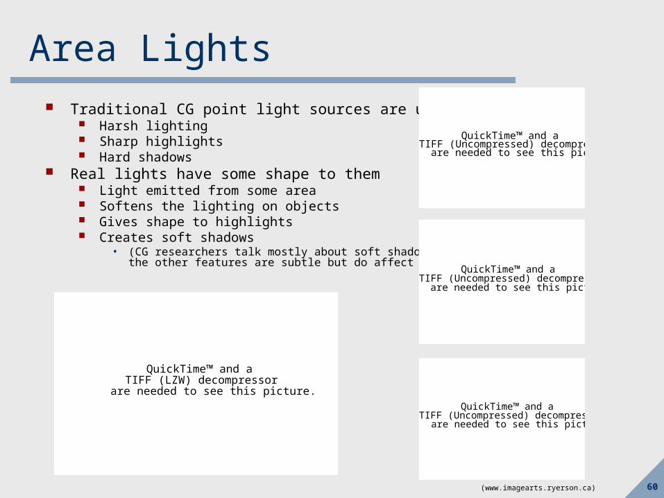
Area Lights Traditional CG point light sources are unrealistic:
Harsh lighting Sharp highlights Hard shadows
Real lights have some shape to them Light emitted from some area Softens the lighting on objects Gives shape to highlights Creates soft shadows
• (CG researchers talk mostly about soft shadows;the other features are subtle but do affect lighting quality)
QuickTime™ and aTIFF (Uncompressed) decompressor
are needed to see this picture.
QuickTime™ and aTIFF (Uncompressed) decompressor
are needed to see this picture.
QuickTime™ and aTIFF (Uncompressed) decompressor
are needed to see this picture.
QuickTime™ and aTIFF (LZW) decompressor
are needed to see this picture.
(www.imagearts.ryerson.ca)

61
QuickTime™ and aTIFF (LZW) decompressor
are needed to see this picture.
Area Lights Instead of having a single direction vector for a light source Send rays distributed across the surface of the light
Each may be blocked by an intervening object Otherwise compute the illumination based on that ray’s direction
Each contributes to the total lighting on the surface point If all rays are blocked, won’t get any light: full shadow (umbra) If some rays blocked, will get some light: penumbra If no rays blocked, fully lit
Notes: Rays distribution should cover surface of the light evenly (though
can be jittered) Hard to create distributions for arbitrary shapes; typically use
lines, disks, rectangles, etc. Can need lots of samples to avoid noise in the penumbra or in
specular highlights
62
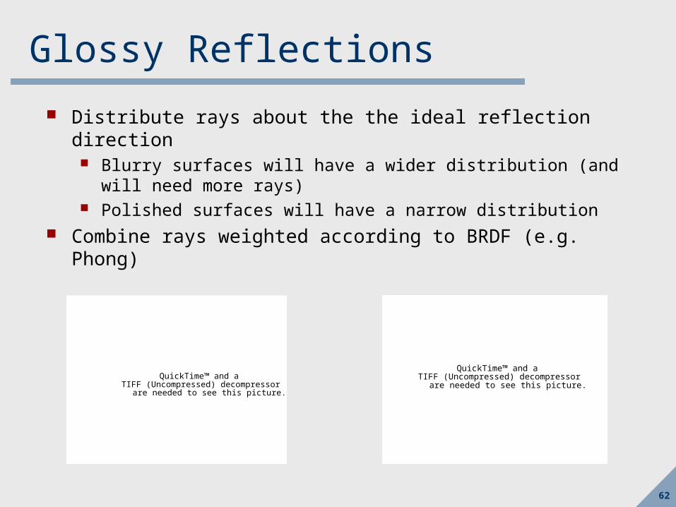
Glossy Reflections
Distribute rays about the the ideal reflection direction Blurry surfaces will have a wider distribution (and
will need more rays) Polished surfaces will have a narrow distribution
Combine rays weighted according to BRDF (e.g. Phong)
QuickTime™ and aTIFF (Uncompressed) decompressor
are needed to see this picture.QuickTime™ and a
TIFF (Uncompressed) decompressorare needed to see this picture.
63
Translucency
Like glossy reflection, but for refraction Distribute rays about the ideal refraction direction
QuickTime™ and aTIFF (Uncompressed) decompressor
are needed to see this picture.
64
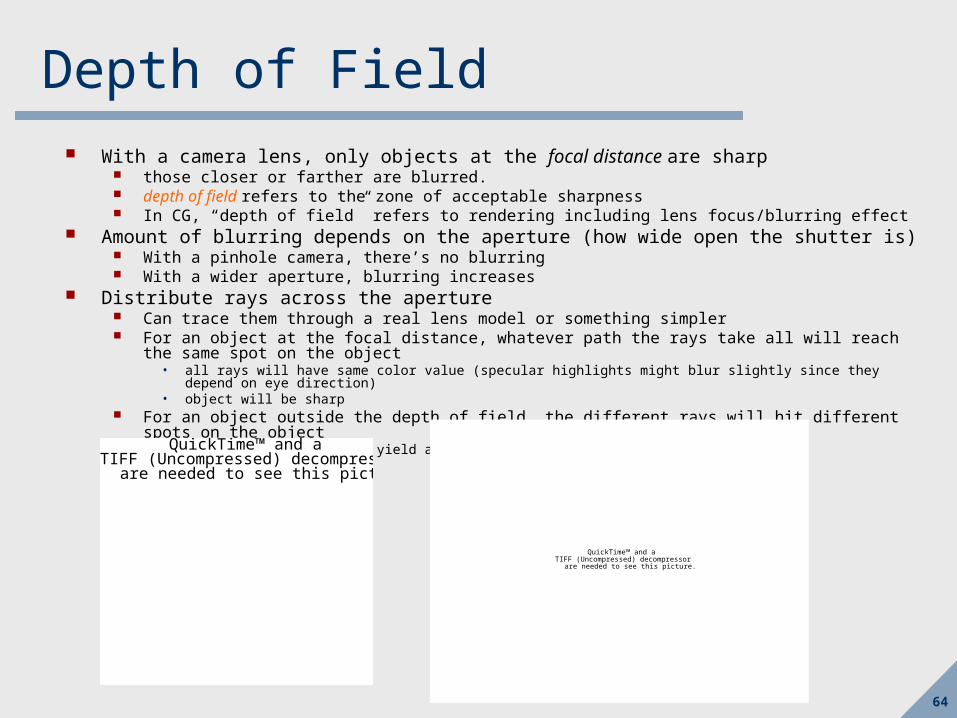
Depth of Field With a camera lens, only objects at the focal distance are sharp
those closer or farther are blurred. depth of field refers to the zone of acceptable sharpness In CG, “depth of field” refers to rendering including lens focus/blurring effect
Amount of blurring depends on the aperture (how wide open the shutter is) With a pinhole camera, there’s no blurring With a wider aperture, blurring increases
Distribute rays across the aperture Can trace them through a real lens model or something simpler For an object at the focal distance, whatever path the rays take all will reach
the same spot on the object• all rays will have same color value (specular highlights might blur slightly since they
depend on eye direction)• object will be sharp
For an object outside the depth of field, the different rays will hit different spots on the object
• combining the rays will yield a blur.
QuickTime™ and aTIFF (Uncompressed) decompressor
are needed to see this picture.
QuickTime™ and aTIFF (Uncompressed) decompressor
are needed to see this picture.
65
Stochastic Ray Tracing
Ray tracing had a big impact on computer graphics in 1980 with the first images of accurate reflections and refractions from curved surfaces
Distribution ray tracing had an even bigger impact in 1984, as it re-affirmed the power of the basic ray tracing technique and added a whole bunch of sophisticated effects, all within a consistent framework
Previously, techniques such as depth of field, motion blur, soft shadows, etc., had only been achieved individually and by using a variety of complex, hacky algorithms
66
Stochastic Ray Tracing Many more rays!
16 samples for antialiasing * 16 samples for motion blur & 16 samples for depth of field * 16 rays for glossy reflections * … ?
Exponential explosion of number of rays Good news: Don’t need extra primary rays per pixel
Can combine distributions E.g. 16 rays in 4x4 jittered supersampling pattern Give each ray a different time and position in the
aperture OK news: Can get by with relatively few secondary rays
For area lights or glossy reflection/refraction 16 primary rays will be combined; each can get by with
only a few secondary rays Still, need more rays.
Slower Insufficient sampling leads to noise Particularly noticeable for soft or blurry features Techniques such as importance sampling to minimize noise
67
Global illumination Take into account bouncing from diffuse objects
Every surface is a light source! Take into account light passing through objects
Caustics Conceptually simple extention to ray tracing:
Send secondary rays in all directions, accumulate all contributions
In practice that would take too many rays, be very noisy Path Tracing
Find multi-step paths from light sources through scene to camera
Monte Carlo Integration: • Numerical techniques to randomly choose rays/paths • Weighting/importance sampling to minimize noise, maximize efficiency
• Photon Maps• Optimize by storing intermediate distribution of light energy
(Also, Radiosity computation: Diffuse light bouncing between all objects Use numerical simultaneous equation solvers)

68
Done
Next class: Final project discussion Upcoming classes: Guest lectures! Cool demos!