Copyright © Cengage Learning. All rights reserved.

13.4 Motion in Space: Velocityand Acceleration

2

Motion in Space: Velocity and Acceleration

In this section we show how the ideas of tangent andnormal vectors and curvature can be used in physics tostudy the motion of an object, including its velocity andacceleration, along a space curve.

In particular, we follow in the footsteps of Newton by usingthese methods to derive Kepler’s First Law of planetarymotion.

3

Motion in Space: Velocity and Acceleration

Suppose a particle moves through space so that itsposition vector at time t is r(t). Notice from Figure 1 that, forsmall values of h, the vector

approximates the direction ofthe particle moving alongthe curve r(t).

Its magnitude measures the sizeof the displacement vector perunit time.

Figure 1

4

Motion in Space: Velocity and Acceleration

The vector (1) gives the average velocity over a timeinterval of length h and its limit is the velocity vector v(t) attime t:

Thus the velocity vector is also the tangent vector andpoints in the direction of the tangent line.

The speed of the particle at time t is the magnitude of thevelocity vector, that is, | v(t) |.

5

Motion in Space: Velocity and Acceleration

This is appropriate because, from (2), we have| v(t) | = | r ʹ′ (t) | = = rate of change of distance withrespect to time

As in the case of one-dimensional motion, the accelerationof the particle is defined as the derivative of the velocity:

a (t) = v ʹ′(t) = r ʹ′ʹ′(t)

6

Example 1The position vector of an object moving in a plane is givenby r (t) = t3 i + t2 j. Find its velocity, speed, and accelerationwhen t = 1 and illustrate geometrically.

Solution:The velocity and acceleration at time t are

v(t) = r ʹ′(t) = 3t2 i + 2t j

a (t) = r ʹ′ʹ′(t) = 6t i + 2 j

and the speed is

7

Example 1 – SolutionWhen t = 1, we have

v(1) = 3 i + 2 j a(1) = 6 i + 2 j | v(1) | =

These velocity and acceleration vectors are shown inFigure 2.

cont’d

Figure 2

8

Motion in Space: Velocity and Acceleration

In general, vector integrals allow us to recover velocitywhen acceleration is known and position when velocity isknown:

If the force that acts on a particle is known, then theacceleration can be found from Newton’s Second Law ofMotion.

The vector version of this law states that if, at any time t, aforce F(t) acts on an object of mass m producing anacceleration a(t), then

F (t) = ma (t)

9

Example 5A projectile is fired with angle ofelevation α and initial velocity v0.(See Figure 6.)

Assuming that air resistance isnegligible and the only externalforce is due to gravity, find theposition function r(t) of the projectile.

What value of α maximizes the range (the horizontaldistance traveled)?

Figure 6

10

Example 5 – SolutionWe set up the axes so that the projectile starts at the origin.Since the force due to gravity acts downward, we have

F = ma = –mg j

Where g = |a | ≈ 9.8 m/s2. Thus

a = –g j

Since vʹ′(t) = a, we have

v(t) = –gt j + C

11

Example 5 – Solutionwhere C = v(0) = v0. Therefore

rʹ′(t) = v(t) = –gt j + v0

Integrating again, we obtain

r(t) = – gt2 j + t v0 + D

But D = r(0) = 0, so the position vector of the projectile isgiven by

r(t) = – gt2 j + t v0

cont’d

12

Example 5 – SolutionIf we write | v0 | = v0 (the initial speed of the projectile), then

v0 = v0 cos α i + v0 sin α j

and Equation 3 becomes

The parametric equations of the trajectory are therefore

cont’d

13

Example 5 – SolutionThe horizontal distance d is the value of x when y = 0.Setting y = 0, we obtain t = 0 or t = (2v0 sin α) / g.This second value of t then gives

Clearly, d has its maximum value when sin 2α = 1, that is,α = 45°.

cont’d

14

Tangential and Normal Components of Acceleration

When we study the motion of a particle, it is often useful toresolve the acceleration into two components, one in thedirection of the tangent and the other in the direction of thenormal.

If we write v = | v | for the speed of the particle, then

and so v = vT

If we differentiate both sides of this equation with respectto t, we get

a = v ʹ′ = v ʹ′T + vT ʹ′

15

Tangential and Normal Components of Acceleration

If we use the expression for the curvature, then we have

The unit normal vector was defined in the precedingsection as N = T ʹ′/| T ʹ′ |, so (6) gives

T ʹ′ = | T ʹ′ |N = vN

and Equation 5 becomes

16

Tangential and Normal Components of Acceleration

Writing aT and aN for the tangential and normal componentsof acceleration, we have

a = aT T + aN Nwhere

aT = v ʹ′ and aN = v2

This resolution is illustratedin Figure 7.

Figure 7

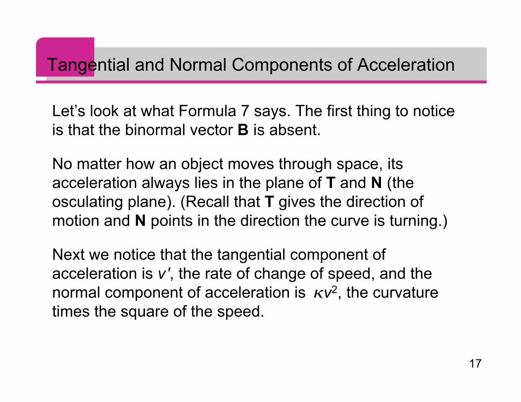
17

Tangential and Normal Components of Acceleration

Let’s look at what Formula 7 says. The first thing to noticeis that the binormal vector B is absent.

No matter how an object moves through space, itsacceleration always lies in the plane of T and N (theosculating plane). (Recall that T gives the direction ofmotion and N points in the direction the curve is turning.)

Next we notice that the tangential component ofacceleration is v ', the rate of change of speed, and thenormal component of acceleration is v2, the curvaturetimes the square of the speed.

18

Tangential and Normal Components of Acceleration

This makes sense if we think of a passenger in a car—asharp turn in a road means a large value of the curvature ,so the component of the acceleration perpendicular to themotion is large and the passenger is thrown against a cardoor.

High speed around the turn has the same effect; in fact, ifyou double your speed, aN is increased by a factor of 4.

Although we have expressions for the tangential andnormal components of acceleration in Equations 8, it’sdesirable to have expressions that depend only on r, r ʹ′,and r ʹ′ʹ′.

19

Tangential and Normal Components of Acceleration

To this end we take the dot product of v = vT with a asgiven by Equation 7:

v a = vT (v ʹ′T + v2N) = vv ʹ′T T + v3T N = vv ʹ′

Therefore

Using the formula for curvature, we have

(since T T = 1 and T N = 0)

20

Example 7A particle moves with position function r (t) = 〈t2, t2, t3〉. Findthe tangential and normal components of acceleration.

Solution: r(t) = t2 i + t2 j + t3 k

rʹ′(t) = 2t i + 2t j + 3t2 k

rʹ′ʹ′(t) = 2 i + 2 j + 6t k

| rʹ′(t) | =

21

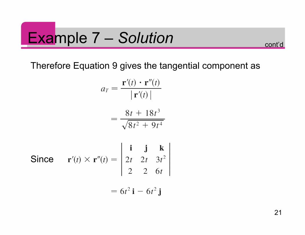
Example 7 – Solution

Therefore Equation 9 gives the tangential component as

Since

cont’d

22

Example 7 – Solution

Equation 10 gives the normal component as

cont’d

23

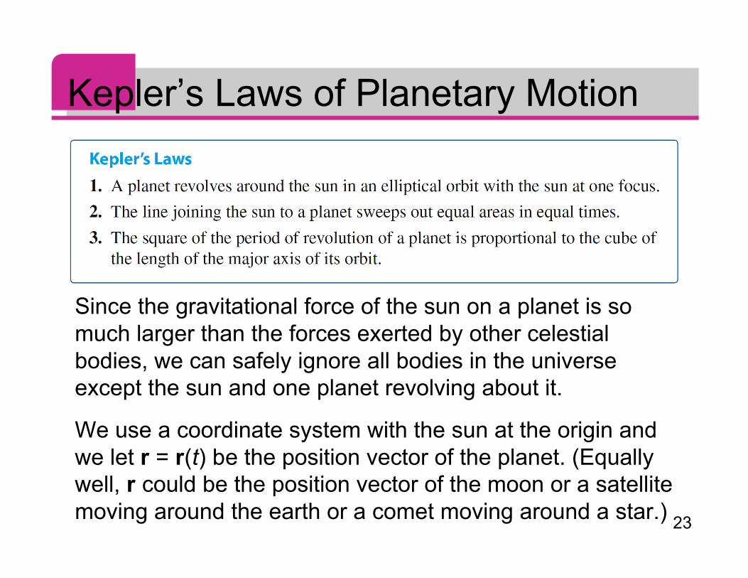
Kepler’s Laws of Planetary Motion

Since the gravitational force of the sun on a planet is somuch larger than the forces exerted by other celestialbodies, we can safely ignore all bodies in the universeexcept the sun and one planet revolving about it.

We use a coordinate system with the sun at the origin andwe let r = r(t) be the position vector of the planet. (Equallywell, r could be the position vector of the moon or a satellitemoving around the earth or a comet moving around a star.)

24

Kepler’s Laws of Planetary MotionThe velocity vector is v = rʹ′ and the acceleration vector isa = rʺ″.

We use the following laws of Newton:

Second Law of Motion: F = ma

Law of Gravitation:

where F is the gravitational force on the planet, m and Mare the masses of the planet and the sun, G is thegravitational constant, r = | r |, and u = (1/r)r is the unitvector in the direction of r.

25

Kepler’s Laws of Planetary MotionWe first show that the planet moves in one plane.

By equating the expressions for F in Newton’s two laws, wefind that

and so a is parallel to r.

It follows that r × a = 0.

26

Kepler’s Laws of Planetary MotionWe use the formula

to write

(r × v) = r ʹ′ × v + r × v ʹ′

= v × v + r × a

= 0 + 0

= 0

27

Kepler’s Laws of Planetary MotionTherefore

r × v = h

where h is a constant vector. (We may assume that h ≠ 0;that is, r and v are not parallel.)

This means that the vector r = r(t) is perpendicular to h forall values of t, so the planet always lies in the plane throughthe origin perpendicular to h.

Thus the orbit of the planet is a plane curve.

28

Kepler’s Laws of Planetary Motion

To prove Kepler’s First Law we rewrite the vector h asfollows:

h = r × v = r × r ʹ′ = r u × (r u)ʹ′ = r u × (r u ʹ′ + r ʹ′u) = r2(u × u ʹ′) + rr ʹ′(u × u) = r2(u × u ʹ′)

Then

a × h = u × (r2u × u ʹ′) = –GM u × (u × u ʹ′)

= –GM [(u u ʹ′)u – (u u)u ʹ′] by Formulaa × (b × c) = (a c)b – (a b)c

29

Kepler’s Laws of Planetary Motion

But u u = | u |2 = 1 and, since | u (t) | = 1, it follows that

u uʹ′ = 0

Therefore

a × h = GM uʹ′

and so (v × h)ʹ′ = vʹ′ × h = a × h = GM uʹ′

30

Kepler’s Laws of Planetary MotionIntegrating both sides of this equation, we get

v × h = GM u + c

where c is a constant vector.

At this point it is convenient to choose the coordinate axesso that the standard basis vector k points in the direction ofthe vector h.

Then the planet moves in the xy-plane. Since bothv × h and u are perpendicular to h, Equation 11 shows thatc lies in the xy-plane.

31

Kepler’s Laws of Planetary MotionThis means that we can choose the x- and y-axes so thatthe vector i lies in the direction of c, as shown in Figure 8.

Figure 8

32

Kepler’s Laws of Planetary MotionIf θ is the angle between c and r, then (r, θ ) are polarcoordinates of the planet.

From Equation 11 we have

r (v × h) = r (GM u + c) = GM r u + r c

= GMr u u + | r | | c | cos θ

= GMr + rc cos θ

where c = | c |.

33

Kepler’s Laws of Planetary MotionThen

where e = c/(GM).

But

r (v × h) = (r × v) h = h h = | h |2 = h2

where h = | h |.

34

Kepler’s Laws of Planetary MotionSo

Writing d = h2/c, we obtain the equation

we see that Equation 12 is the polar equation of a conicsection with focus at the origin and eccentricity e. We knowthat the orbit of a planet is a closed curve and so the conicmust be an ellipse.