1.258J Lecture 11 , Ridership prediction - MIT OpenCourseWare · Alternative approaches to route...

- - -

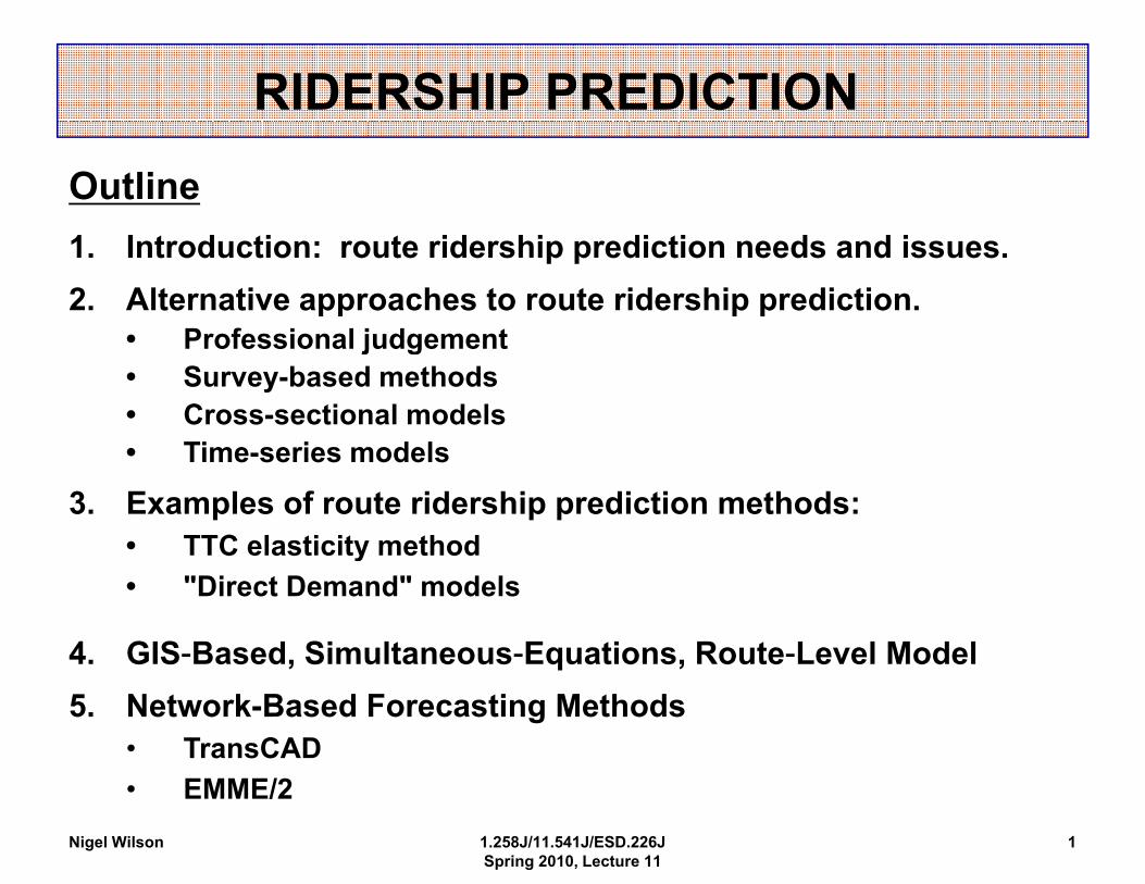
Outline 1. Introduction: route ridership prediction needs and issues. 2. Alternative approaches to route ridership prediction.

•• Professional judgementProfessional judgement • Survey-based methods • Cross-sectional models • Ti i d lTime-series models

3. Examples of route ridership prediction methods: • TTC elasticity methodTTCelasticity method • "Direct Demand" models

4. GIS-Based Simultaneous-Equations Route-Level Model GIS Based, Simultaneous Equations, Route Level Model 5. Network-Based Forecasting Methods

• TransCAD • EMME/2

Nigel Wilson 1.258J/11.541J/ESD.226J Spring 2010, Lecture 11

4

1

RIDERSHIP PREDICTION

1. as a result of fare

a e e ast c t ca cu at o

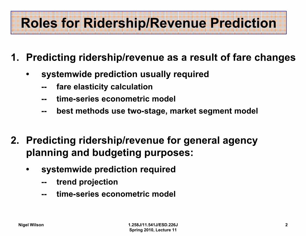
1. Predicting ridership/revenue as a result of fare changesPredicting ridership/revenue changes • systemwide prediction usually required

-- fare elasticityy calculation

-- time-series econometric model-- best methods use two-stage, market segment model

2. Predicting ridership/revenue for general agency planning and budgeting purposes: • systemwide prediction required

-- trend projection

-- time-series econometric model


2

Roles for Ridership/Revenue Prediction

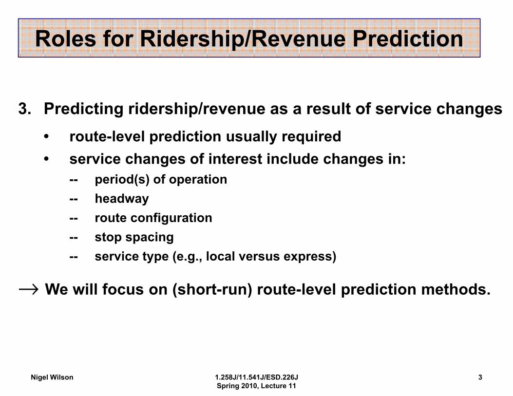
3. Predicting ridership/revenue as a result of service changes

• route-level prediction usually required • service changes of interest include changes in:

-- period(s) of operation

-- headwayheadway

-- route configuration

-- stop spacing

-- service type (e.g., local versus express)

→We will focus on (short-run) route-level prediction methods. →We will focus on (short run) route level prediction methods.


3

Roles for Ridership/Revenue Prediction

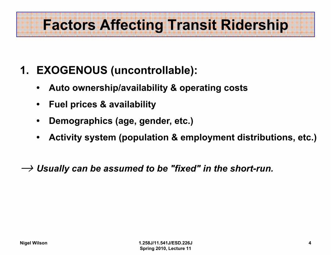
1. EXOGENOUS (uncontrollable): • Auto ownership/availability & operating costs

• Fuel prices & availability

• Demographics (age, gender, etc.)

• Activity system (population & employment distributions, etc.)

→ Usually can be assumed to be "fixed" in the short-run.


4

Factors Affecting Transit Ridership

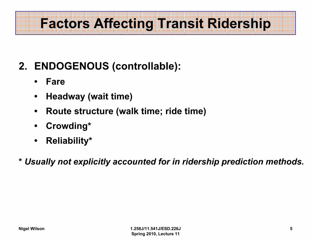
2. ENDOGENOUS (controllable): • Fare • Headway (wait time) • Route structure (walk time; ride time) • Crowding* • Reliability*

* Usually not explicitly accounted for in ridership prediction methods.


5

Factors Affecting Transit Ridership

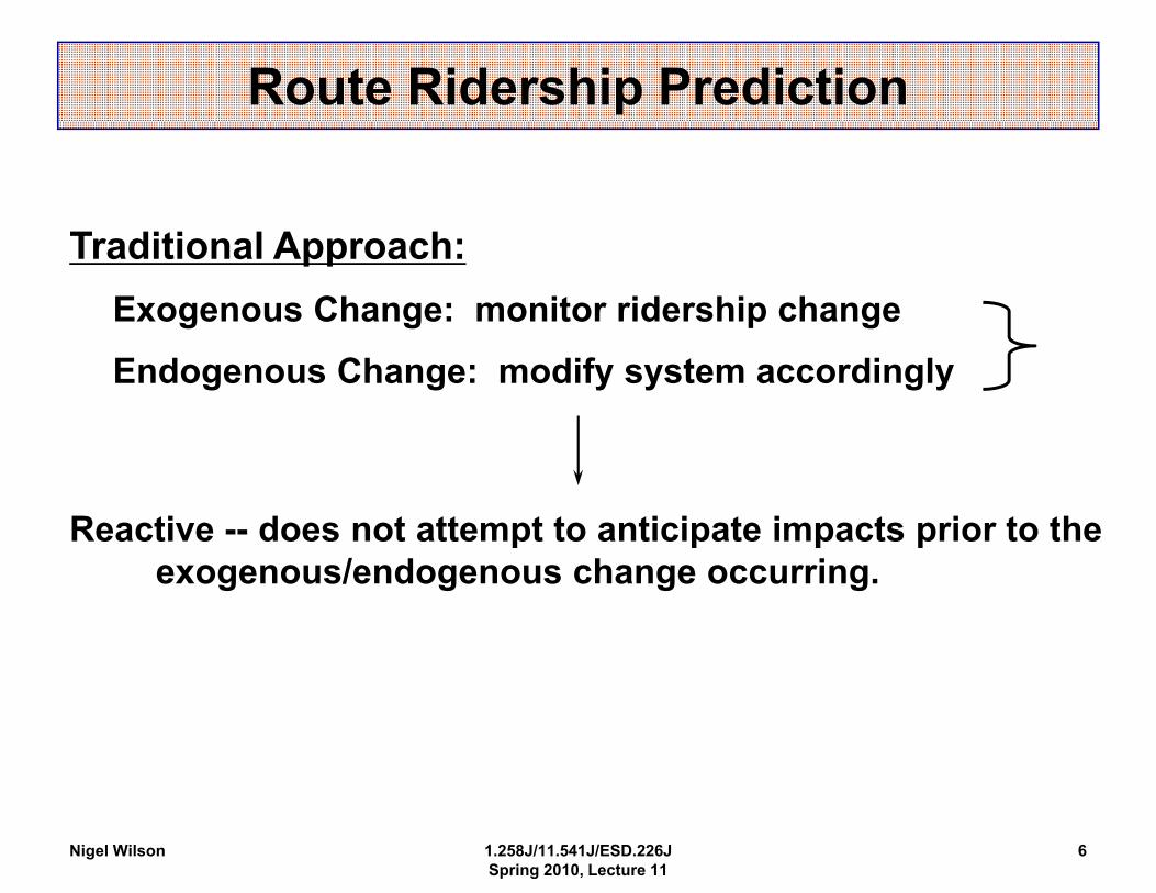
Traditional Approach: Exogenous Change: monitor ridership change

Endogenous Change: modify system accordingly

Reactive -- does not attempt to anticipate impacts prior to the exogenous/endogenous change occurring.


6

Route Ridership Prediction

Current Practice:

• Little attention given to the problem in many agencies, except for fare changes and major capital projects

• Traditional urban transport planning models inappropriate and ineffective (generally not detailed enough and too complex to run repeatedly)

• Ad-hoc, judgemental methods dominate


7

Route Ridership Prediction

1. Professional judgement

2. Non-committal survey techniques

3. Cross-sectional data models

4 TiTimeme-seriesseries datadata modelsmodels4.


8

Approaches to Predicting Route Ridership

• Widely used for a variety of changes • Based on experience & local knowledge • No evidence of accuracy of method (or reproducibility

of results) • Reflects:

- lack of faith in formal models

- lack of data and/or technical expertise to support the development of formal models

- relative unimportance of topic to many properties (compared to impact of changes on existing passengers)


9

Professional Judgement

A. Non-Committal Surveys 1. Survey potential riders to ask how they would respond

t th i ( i h )to the new service (or service change)

2. Extrapolate to total population by applying survey responses at the market segment levelresponses at the market segment level.

3. Adjust for "non-committal bias" by multiplying by an apppproppriate adjjustment factor ((which can rangge in practice from 0.05 to 0.50).

---> NOT generally recommended.NOT generally recommended.


10

Survey-Based Methods

t

B. Stated Preference Surveys • "Stated preference measurement" (conjoint analysis) is

emerging as a viablble stati tistical tool f l for assessing likelyi i t ti l t i lik l responses to proposed transportation system changes

-- i l d t il d i d i & d involves detailed, rigorous survey designs & datta analyses

-- usually involves a series of tradeoffs that allows aa series of tradeoffs that allows ausually involves planner to rank relative importance of different types of improvements

-- may bbe partiicullarlly useffull f for new serviices or new service areas


11

Survey-Based Methods

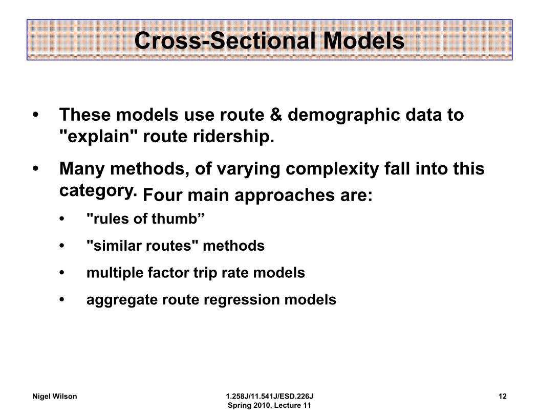
• These models use route & demographic data to "explain" route ridership.

• Many methods, of varying complexity fall into this category. Four main approaches are: • "rules of thumb”

• "similar routes" methods

• multiple factor trip rate models

• aggregate route regression models


12

Cross-Sectional Models

ersh

ipR

ide

Frequency

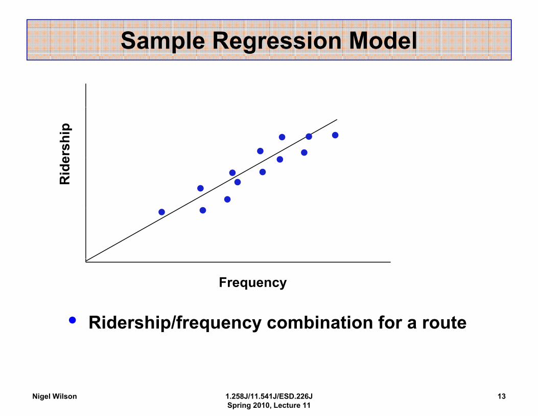
• Ridership/frequency combination for a route


13

Sample Regression Model

Transit Demand Curves and Scheduler’s Rule

SS

P4 D4

DD33 P3

D2

PP2 D1 P1

Rid

ershh

ip

Frequency

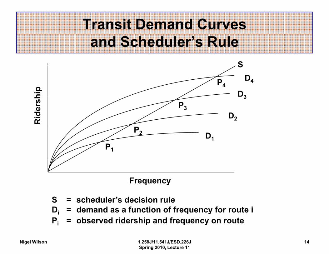
S = scheduler’s decision rule Di = demand as a function of frequency for route i PPi == observed ridership and frequency on route observed ridership and frequency on route


14

t t t t t

Typical Transit Elasticities

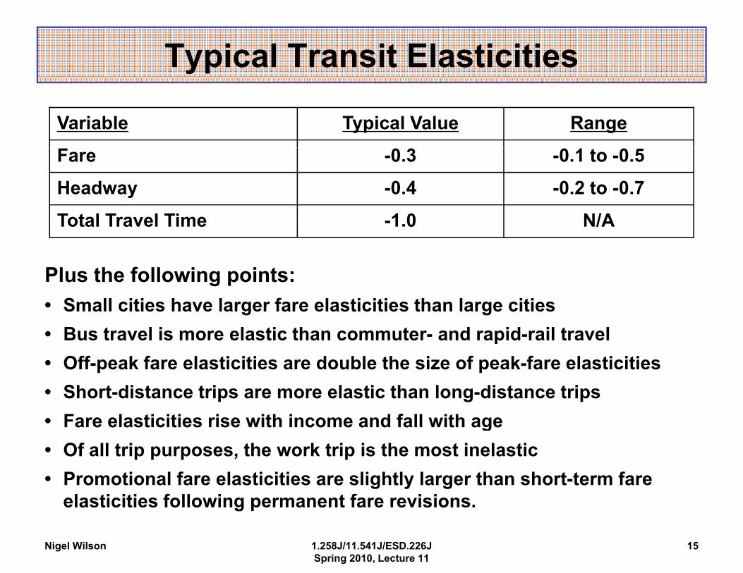
Variable Typical Value Range

Fare -0.3 -0.1 to -0.5

Headway -0.4 -0.2 to -0.7

Total Travel Time Total Travel Time 1 0-1.0 N/AN/A

Plus the following points: • Small cities have larger fare elasticities than large cities • Bus travel is more elastic than commuter- and rapid-rail travel • Off k f l i i i d bl h i f k f l i iOff-peak fare elasticities are double the size of peak-fare elasticitiies • Short-distance trips are more elastic than long-distance trips • Fare elasticities rise with income and fall with ageFare elasticities rise with income and fall with age • Of all trip purposes, the work trip is the most inelastic • Promotional fare elasticities are slightly larger than short-term fare

ellasti iti ticities ffoll llowiing permanent f t fare revisions.i i

Nigel Wilson 1.258J/11.541J/ESD.226J 15 Spring 2010, Lecture 11

Usage of Route Ridership Prediction Methods

Number of ridership estimation methods used by operators (1990 survey)

Number of Methods Operators One Two Three Four Total Count 18 15 5 1 39 Percent 46% 38% 13% 3% 100%

Number of operators reporting use of each type of ridership forecasting method (1990 survey)method (1990 survey)

Forecasting Method

Operators Judgement Non-committal Survey Similar Routes Rules of Thumb CountCount 1717 44 1010 1010 Percent 44% 10% 26% 26% Change from 1982 23% -5% 3% -10%

F ti M th dForecasting Method Operators Linear Regression Elasticity Non-Forecasting Other Count 5 12 7 4 Percent 13% 31% 18% 10% Change from 1982 8% 21% -3% -8%


16

t t t

=

TTC Elasticity Method

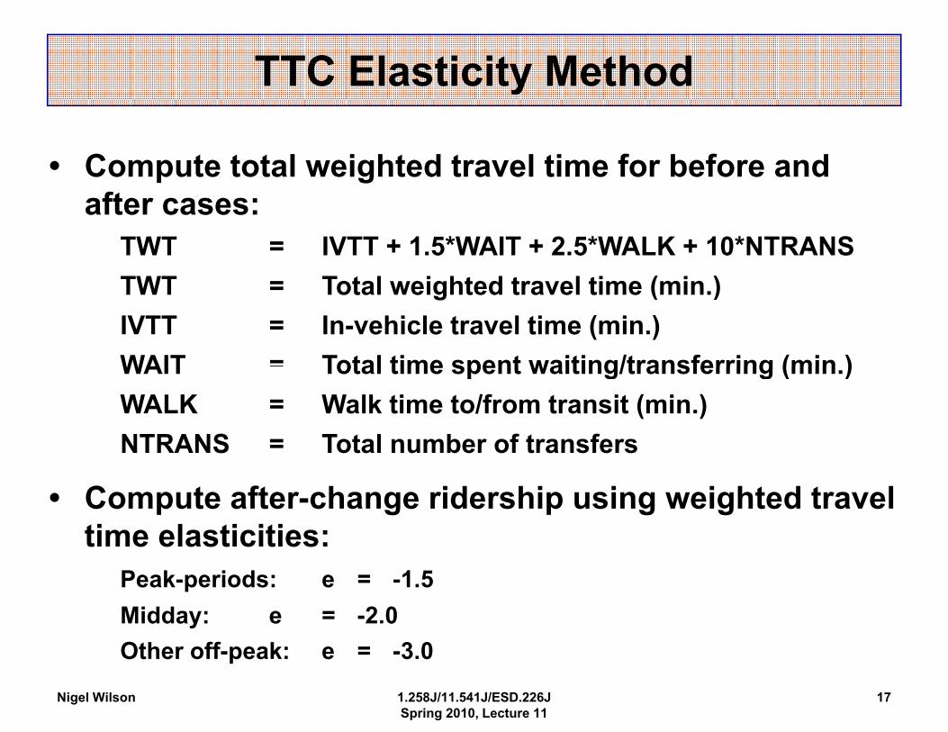
• Compute total weighted travel time for before and after cases:

TWT = IVTT + 1.5*WAIT + 2.5*WALK + 10*NTRANS TWTTWT = T t l i h d l i ( iTotal weighted travel time (min.)) IVTT = In-vehicle travel time (min.) WAIT = Total time spent waiting/transferring (min.)WAIT Total time spent waiting/transferring (min )WALK = Walk time to/from transit (min.)NTRANS = Total number of transfers

• Compute after-change ridership using weighted travel time elasticities:time elasticities:

Peak-periods: e = -1.5

Midday: e = -2.0

Other off-peak: e = -3.0


17

•

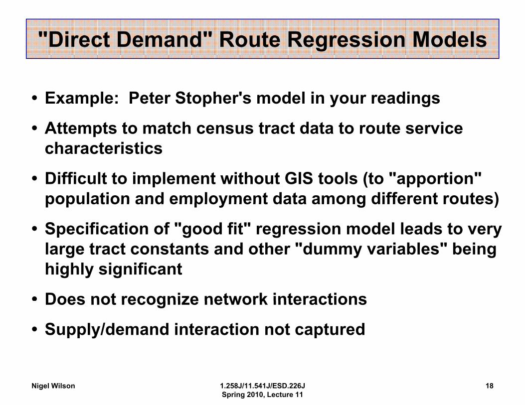
"Direct Demand" Route Regression Models

• Exampple: Peter Stoppher's model in yyour readinggs

• Attempts to match census tract data to route service characteristicscharacteristics

• Difficult to implement without GIS tools (to "apportion" population and employment data among different routes)population and employment data among different routes)

• Specification of "good fit" regression model leads to very large tract constants and other "dummy variables" beinglarge tract constants and other dummy variables being highly significant

• Does not recognize network interactionsDoes not recognize network interactions

• Supply/demand interaction not captured


18

t

Alternative Approaches to the Rid hi F ti P bl Ridership Forecasting Problem

• GIS-based, simultaneous-equation, route-level models:- capable of including competing/ complementary routes

bl t dd d d l i t ti - able to address demand-supply interactions

- "logical next step" beyond Stopher-type model

• F ll Full networkk moddells: - explicitly deal with competing/complementary routes - able to include trip distribution and mode split effects able to include trip distribution and mode split effects

- "logical next step" beyond TTC-type model

→ B th h i t i d t ti Both approaches require a computerized representation off the transit network and the service area.

This is usually achieved through some form of Geographic This is usually achieved through some form of Geographic Information System (GIS).


19

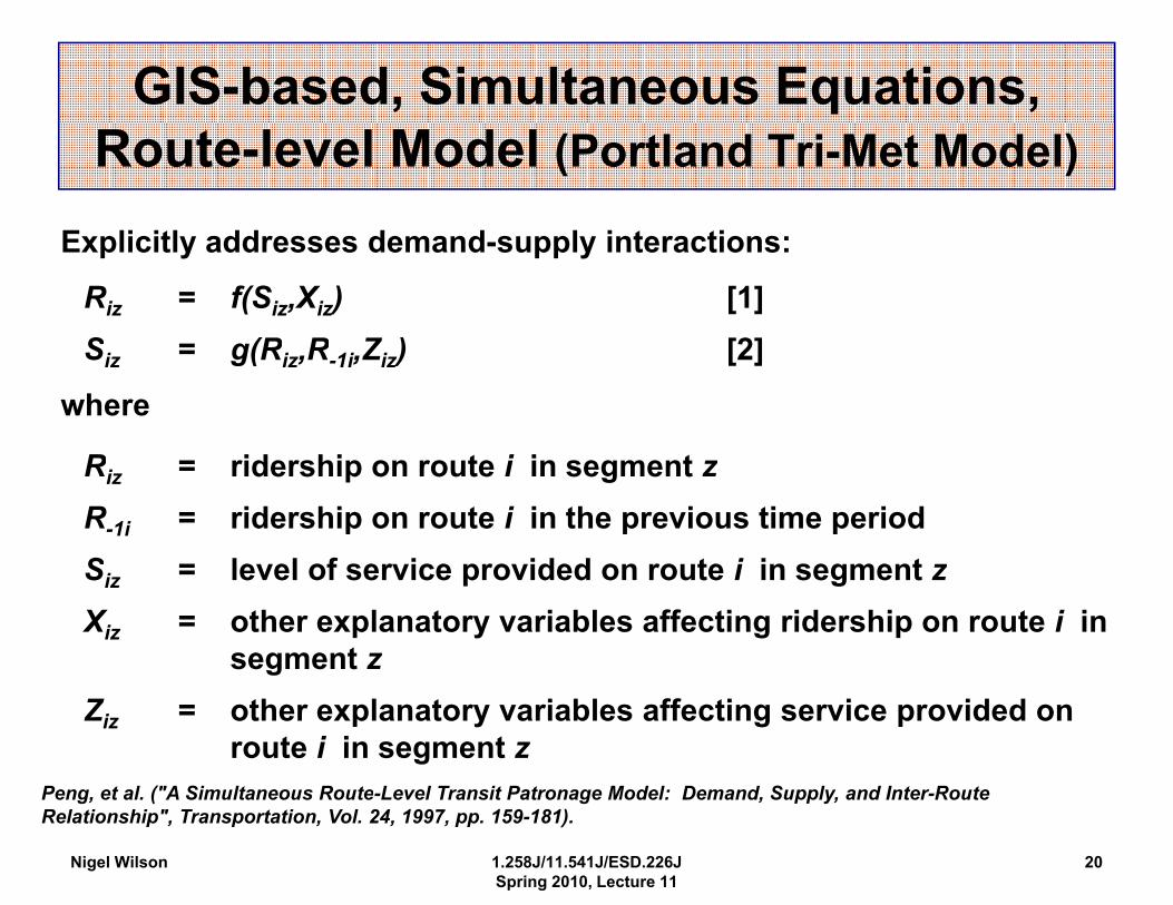
GIS-based, Simultaneous Equations, Route-level Model (Portland Tri-Met Model)

E li itl dd d d l i t ti Explicitly addresses demand-supply interactions:

Riz = f(Siz,Xiz) [1]S (R R Z ) [2]Siz = g(Riz,R-1i,Ziz) [2]

where

Riz = ridership on route i in segment z

R-1i = ridership on route i in the previous time period

S = l l f i id d t i iSiz level of service provided on route i in segmentt z Xiz = other explanatory variables affecting ridership on route i in

seggment z Ziz = other explanatory variables affecting service provided on

route i in segment z Peng, et al. ("A Simultaneous Route-Level Transit Patronage Model: Demand, Supply, and Inter-Route Relationship", Transportation, Vol. 24, 1997, pp. 159-181).


20

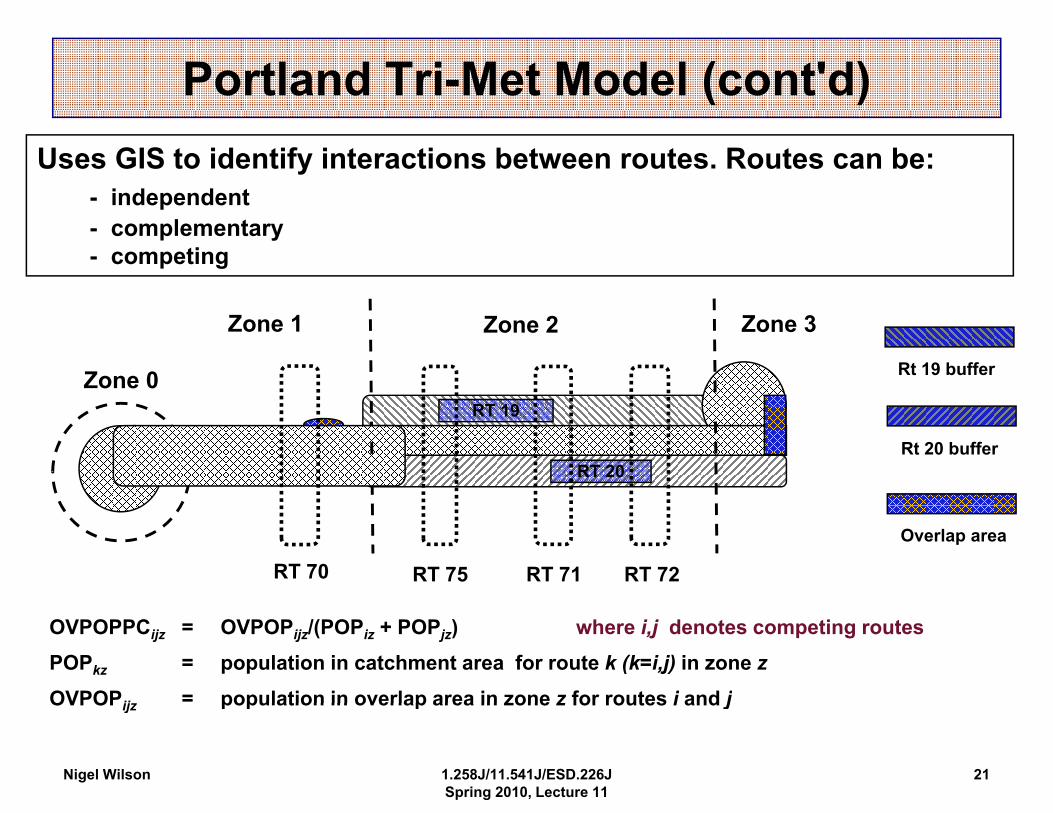
Portland Tri-Met Model (cont'd) Uses GIS to identify interactions between routes. Routes can be:

- independentp- complementary - competing

Zone 1 Zone 3Zone 2

Zone 0 RT 19 RT 19

RT 20

Rt 19 buffer

Rt 20 buffer

Overlap area

RT 70 RT 75 RT 71 RT 72

OVPOPPCijz = OVPOPijz/(POPiz + POPjz) where i,j denotes competing routes

POPkz = population in catchment area for route k (k=i,j) in zone z

OVPOPij = population in overlap area in zone z for routes i and jOVPOPijz population in overlap area in zone z for routes i and j

Nigel Wilson 1.258J/11.541J/ESD.226JSpring 2010, Lecture 11

21

To inter route and

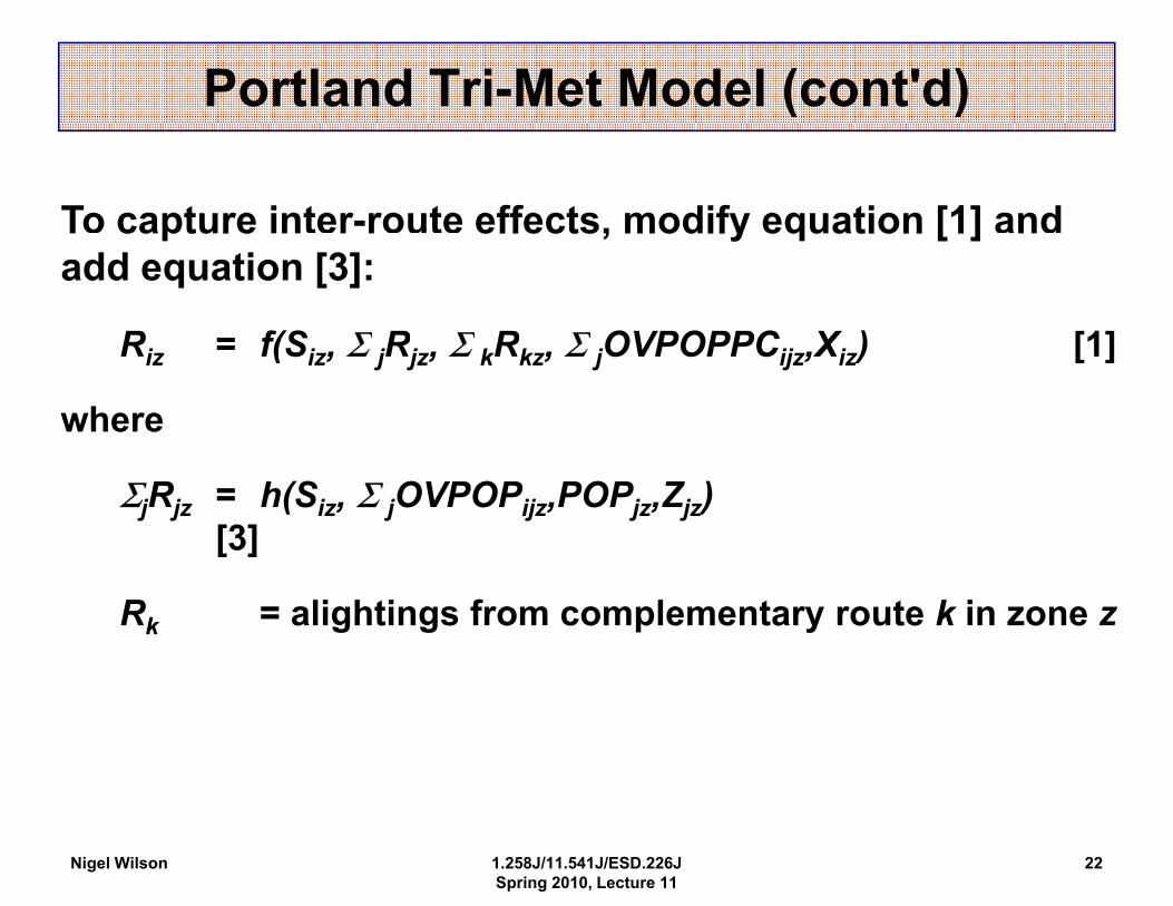
Portland Tri-Met Model (cont'd)

To capture inter-route effects, modify equation [1] andcapture effects, modify equation [1] add equation [3]:

R == f(Sf(Siz, ΣΣ jRRjz, Σ kRRkz, ΣΣ jOVPOPPCOVPOPPCijz,XXiz) [1]Riz Σ ) [1]

where

ΣjRjz = h(Siz, Σ jOVPOPijz,POPjz,Zjz) [3]

Rk = alightings from complementary route k in zone z


22

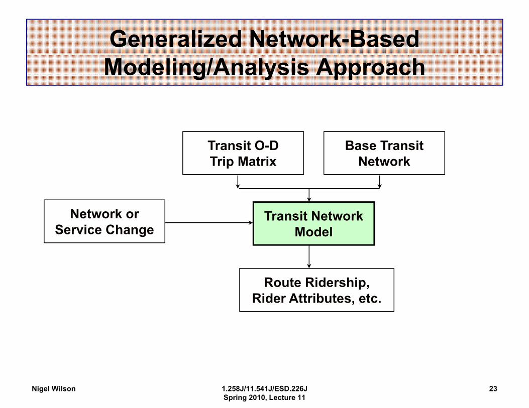
Generalized Network-Based Modeling/Analysis Approach

Transit O-D Base Transit Trip Matrix Network

Network or Transit Network Service Change Model

Route Ridership, Rider Attributes,, etc.


23

Three Levels of

-

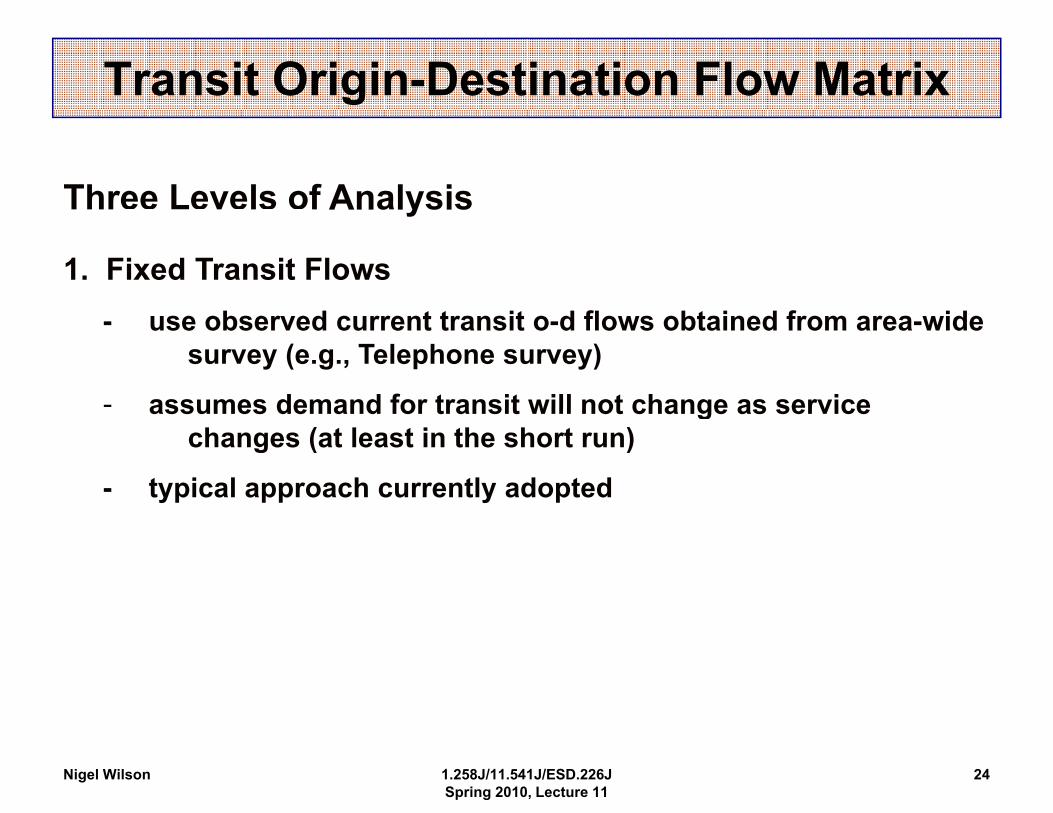
Transit Origin-Destination Flow Matrix

Three Levels of AnalysisAnalysis

1. Fixed Transit Flows - use observed current transit o-d flows obtained from area-wide

survey (e.g., Telephone survey)

- assumes demand for transit will not change as serviceassumes demand for transit will not change as service changes (at least in the short run)

- typical approach currently adopted


24

Three Levels of

&

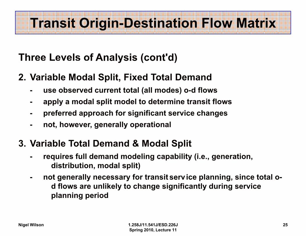
Transit Origin-Destination Flow Matrix

Three Levels of Analysis (cont'd)Analysis (cont d)

2. Variable Modal Split, Fixed Total Demand - use observed current total (all modes) o d flows use observed current total (all modes) o-d flows - apply a modal split model to determine transit flows - preferred approach for significant service changes - not, however, generally operational

3. Variable Total Demand & Modal Spplit - requires full demand modeling capability (i.e., generation,

distribution, modal split)- nott generall lly necessary ffor ttransitit serv iice pllanniing, siince ttottall o-

d flows are unlikely to change significantly during service planning period


25

Examples Of Transit Network Modeling & Analysis Packages

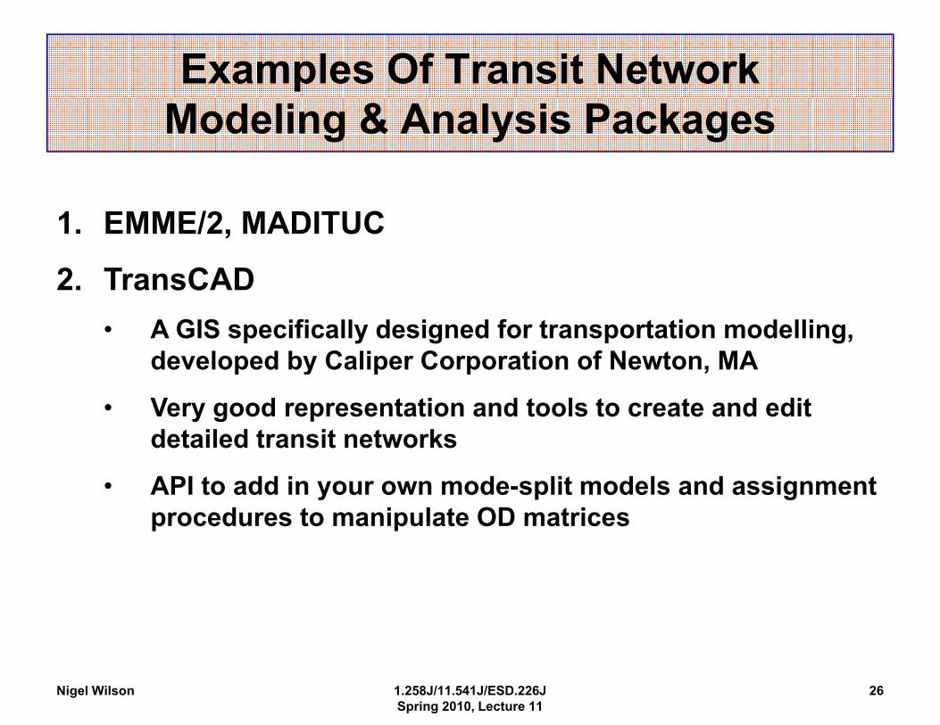
1. EMME/2, MADITUC

22. TransCAD TransCAD • A GIS specifically designed for transportation modelling,

developed by Caliper Corporation of Newton MA developed by Caliper Corporation of Newton, MA

• Very good representation and tools to create and edit detailed transit networks

• API to add in your own mode-split models and assignment procedures to manipulate OD matrices


26

Examples Of Transit Network Modeling d A l i P kand Analysis Packages

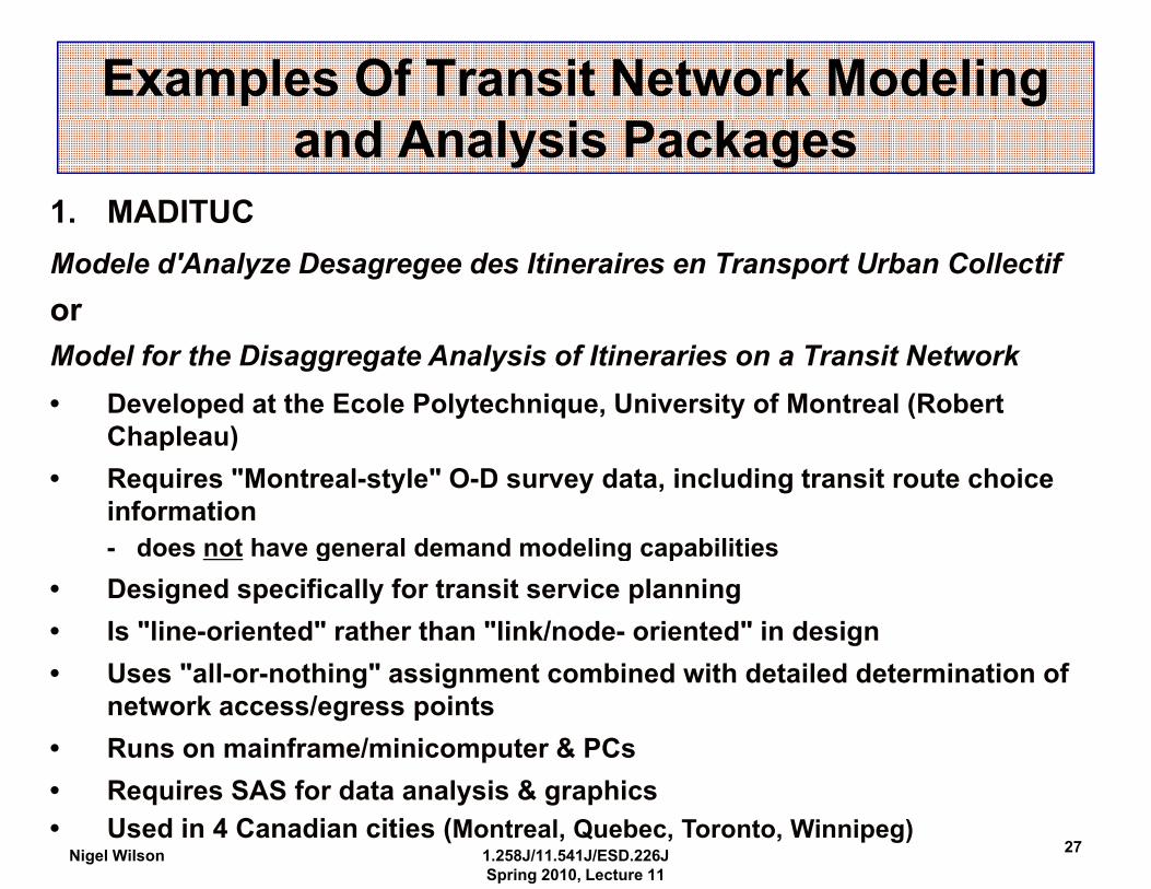
1. MADITUC Modele d'Analyze Desagregee des Itineraires en Transport Urban Collectif or Model for the Disaggregate Analysis of Itineraries on a Transit Network • Developed at the Ecole Polytechnique, University of Montreal (Robert

Chapleau)Chapleau) • Requires "Montreal-style" O-D survey data, including transit route choice

information - does not have general demand modeling capabilities does not have general demand modeling capabilities

• Designed specifically for transit service planning • Is "line-oriented" rather than "link/node- oriented" in design • Uses "all-or-nothing" assignment combined with detailed determination of

network access/egress points • Runs on mainframe/minicomputer & PCs • Requires SAS for data analysis & graphics

Nigel Wilson 1.258J/11.541J/ESD.226J • Used in 4 Canadian cities (Montreal, Quebec, Toronto, Winnipeg)

Spring 2010, Lecture 11

27

t

- -

Examples of Transit Network Modeling and A l i P k 'd Analysis Packages, cont'd

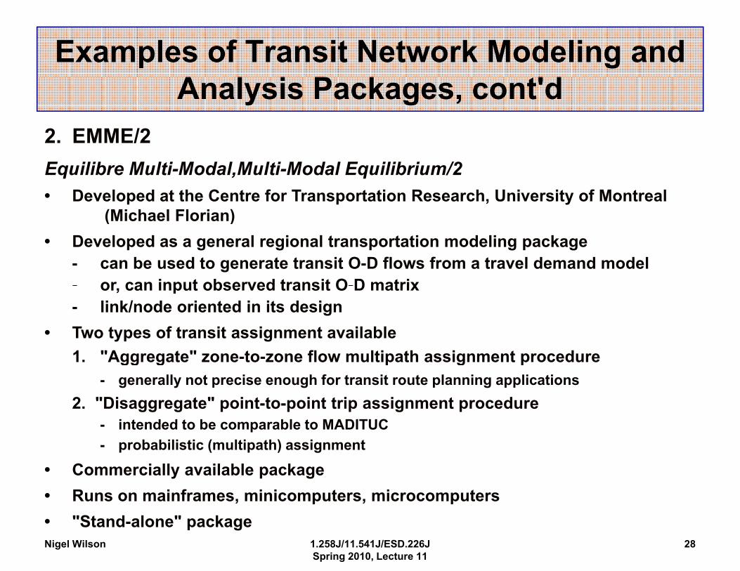
2. EMME/2 Equilibre Multi-Modal,Multi-Modal Equilibrium/2 • Developed at the Centre for Transportation Research, University of Montreal

(Michael Florian)(Michael Florian) • Developed as a general regional transportation modeling package

- can be used to generate transit O-D flows from a travel demand model - oror, can input observed transit O D matrixcan input observed transit O-D matrix - link/node oriented in its design

• Two types of transit assignment available 11. "AggregateAggregate" zone to zone flow multipath assignment procedure zone-to-zone flow multipath assignment procedure

- generally not precise enough for transit route planning applications 2. "Disaggregate" point-to-point trip assignment procedure

- intended to be comparable to MADITUCintended to be comparable to MADITUC

- probabilistic (multipath) assignment

• Commercially available package •• Runs on mainframes minicomputers microcomputers Runs on mainframes, minicomputers, microcomputers • "Stand-alone" package Nigel Wilson 1.258J/11.541J/ESD.226J

Spring 2010, Lecture 11 28

Interactive for network

TransCAD Network Model Capabilities

• Interactive computer graphics for network editingcomputer graphics editing and display

• Network database management systemNetwork database management system

• Network assignment procedure

• Flexible display & output of results & base data - plots & reports

- screen displays, printer & plotter hard copies


29

Geocoded transit links & nodes

t

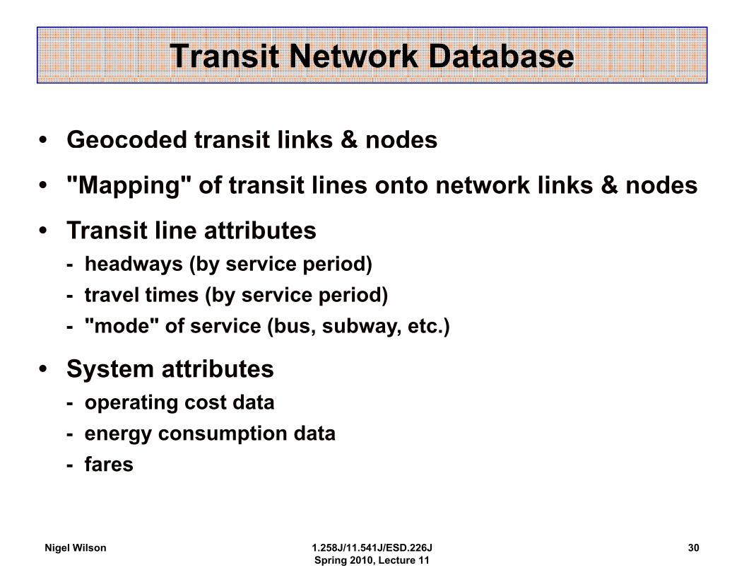
Transit Network Database

• Geocoded transit links & nodes

• "Mapping" of transit lines onto network links & nodes

• Transit line attributes - headways (by service period) - l ti (b i i d)travel times (by service period)- "mode" of service (bus, subway, etc.)

• System attributes - operating cost data - energy consumptition ddatta - fares


30

-

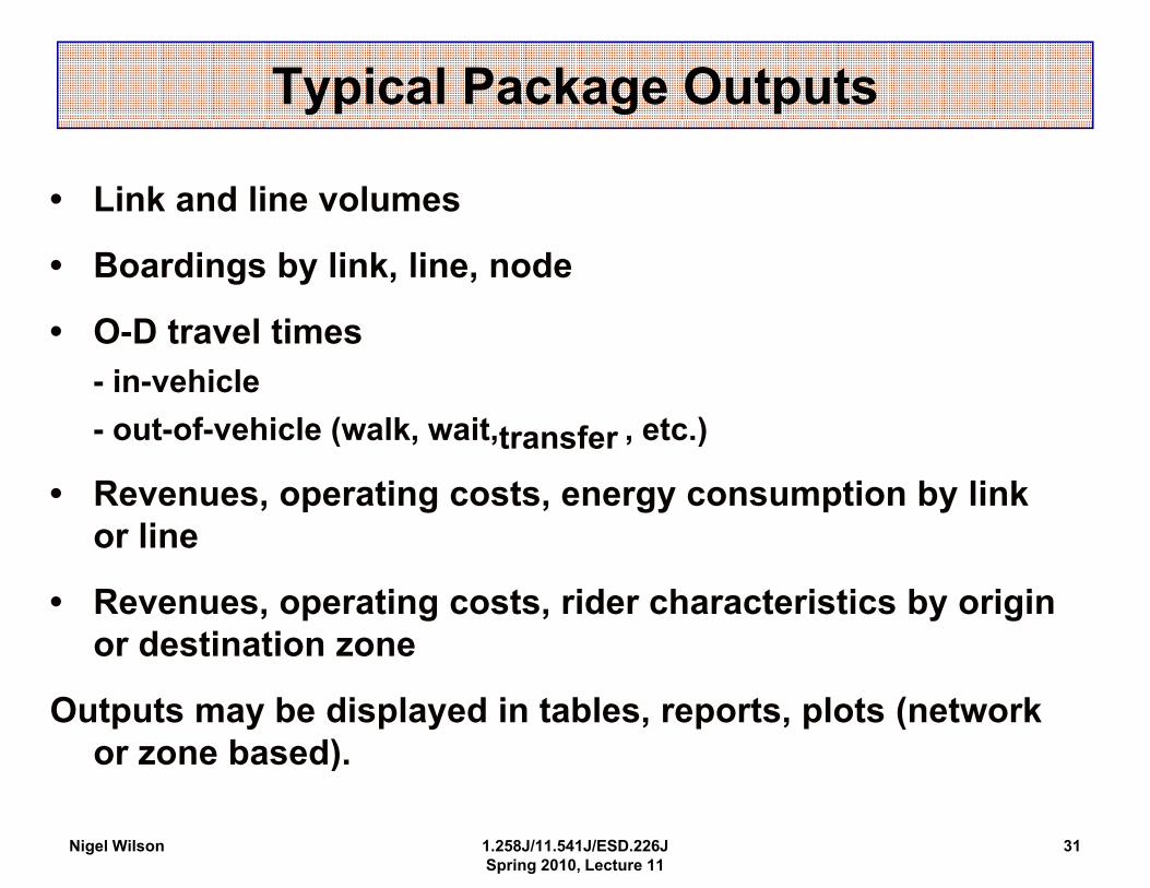
Typical Package Outputs

• Link and line volumes

• Boardings by link, line, node

• OO-D travel timesD travel times - in-vehicle - out-of-vehicle ((walk,, wait,, transfer ,, etc.))

• Revenues, operating costs, energy consumption by link or line

• Revenues, operating costs, rider characteristics by origin or destination zone

Outputs may be displayed in tables, reports, plots (network or zone based)).


31

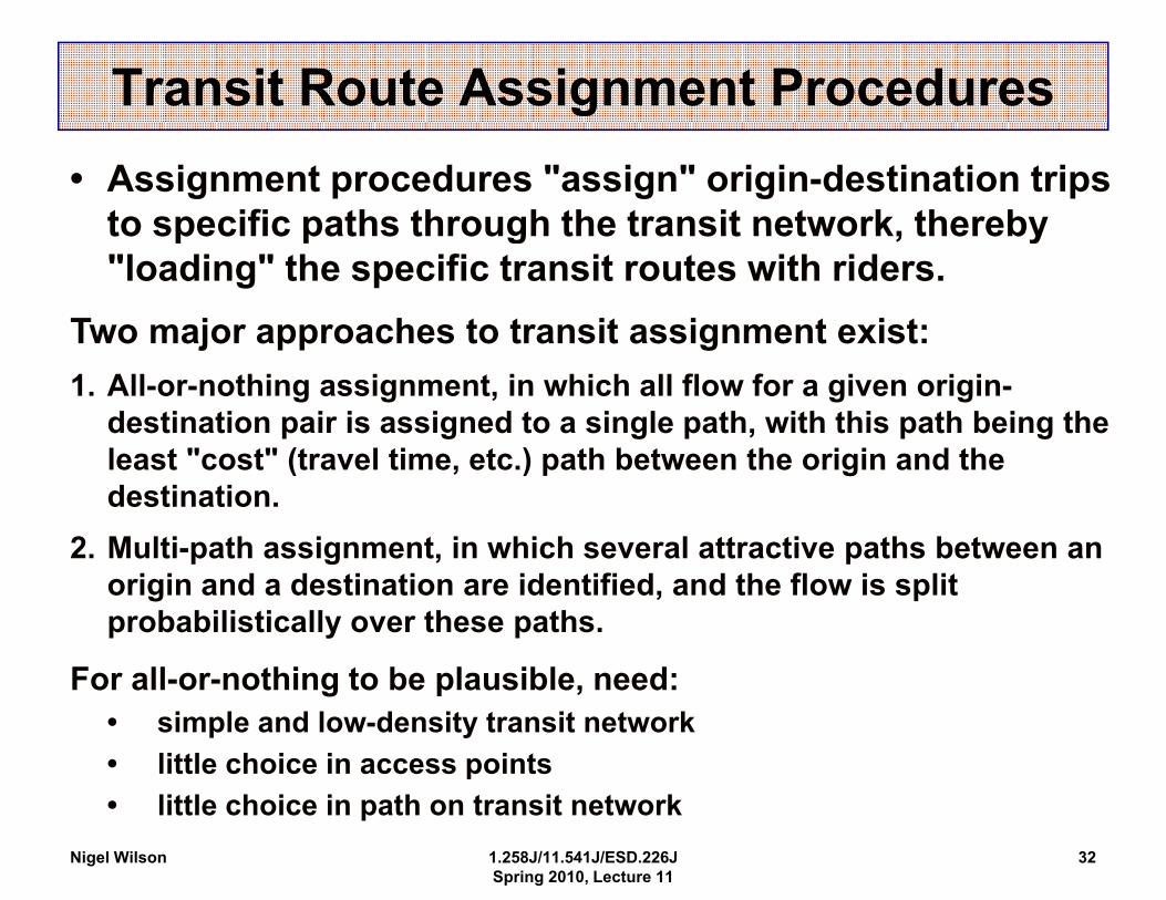
Transit Route Assignment Procedures • Assignment procedures "assign" origin-destination trips

to specific paths through the transit network, therebyto specific paths through the transit network, thereby "loading" the specific transit routes with riders.

Two major approaches to transit assignment exist:Two major approaches to transit assignment exist: 1. All-or-nothing assignment, in which all flow for a given origin-

destination pair is assigned to a single path, with this path being the l t " t" (t l ti t ) th b t th i i d th least "cost" (travel time, etc.) path between the origin and the destination.

2. Multi-ppath assiggnment,, in which several attractive ppaths between an origin and a destination are identified, and the flow is split probabilistically over these paths.

F ll thi t b l ibl dFor all-or-nothing to be plausible, need: • simple and low-density transit network • little choice in access ppoints • little choice in path on transit network


can also be either:

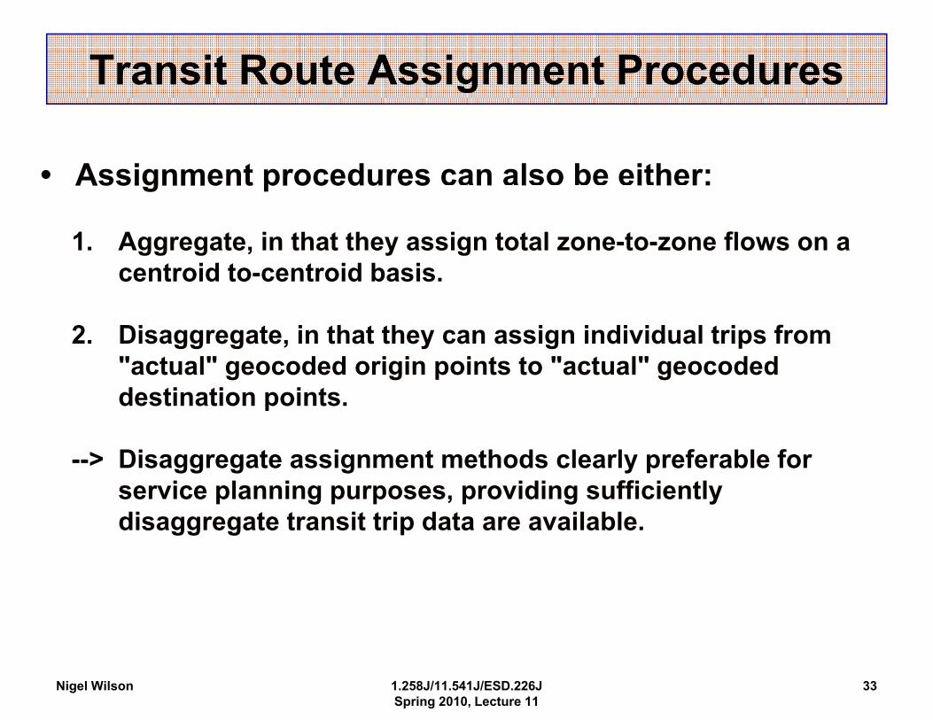
Transit Route Assignment Procedures

• Assignment procedures can also be either:Assignment procedures

1. Aggregate, in that they assign total zone-to-zone flows on a centroid to centroid basis centroid to-centroid basis.

2. Disaggregate, in that they can assign individual trips from ""acttual" geocodded ori iigin poii tnts tto ""acttual" geocoddedl" d l" d destination points.

--> Disaggregate assignment methods clearly preferable for service planning purposes, providing sufficiently disaggggreggate transit tripp data are available.


33

=

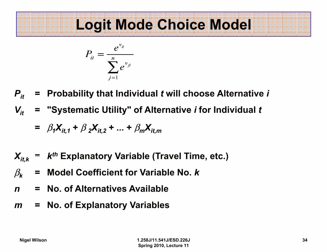
Logit Mode Choice Model

Pit = Probability that Individual t will choose Alternative iPit Probability that Individual t will choose Alternative i

Vit = "Systematic Utility" of Alternative i for Individual t

== β X + β X + + β Xβ1Xit,1 + β 2Xit,2 + ... + βmXit,m

X = kkth Explanatory Variable (Travel Time etc )Xit,k Explanatory Variable (Travel Time, etc.)

βk = Model Coefficient for Variable No. k

n = NoNo. ofof AlternativesAlternatives Available Availablen =

m = No. of Explanatory Variables


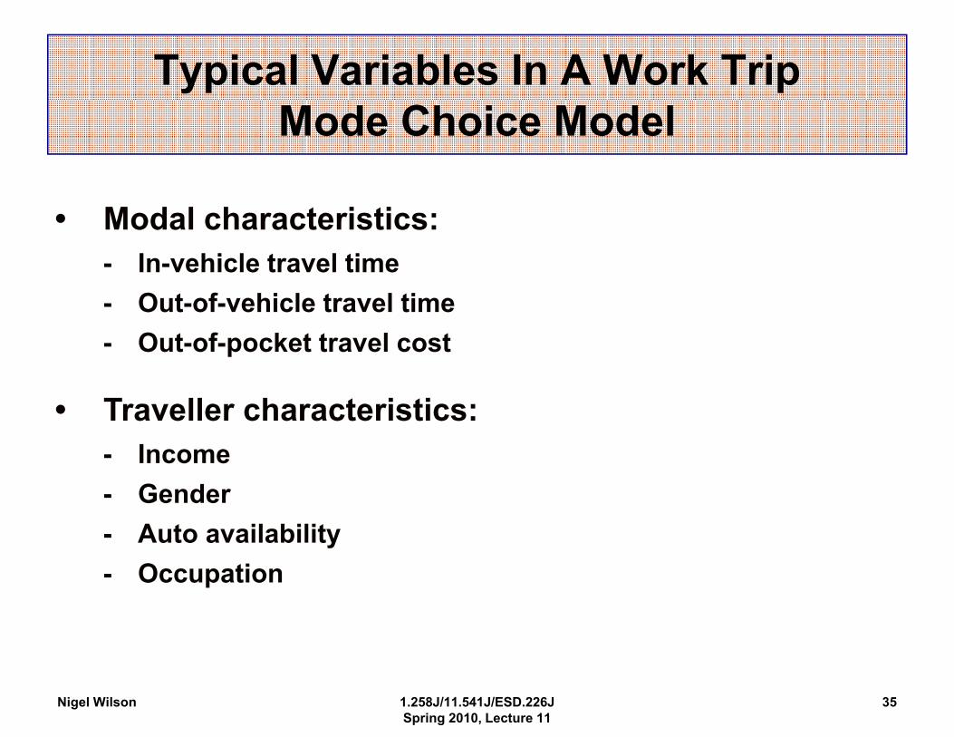
Typical Variables In A Work Trip Mode Choice Model

• Modal characteristics: - In-vehicle travel time - Out-of-vehicle travel time - Out-of-pocket travel cost

• Traveller characteristics: - IncomeIncome

- Gender

- Auto availabilityy

- Occupation


35

MIT OpenCourseWarehttp://ocw.mit.edu

1.258J / 11.541J / ESD.226J Public Transportation SystemsSpring 2010

For information about citing these materials or our Terms of Use, visit: http://ocw.mit.edu/terms.

http://ocw.mit.edu

http://ocw.mit.edu/terms

1.258J Lecture 11 , Ridership prediction - MIT OpenCourseWare · Alternative approaches to route...

Documents

Transcript of 1.258J Lecture 11 , Ridership prediction - MIT OpenCourseWare · Alternative approaches to route...