12-15 Sexual Selection, Conspicuous Consumption and ... · sexual selection, conspicuous...

ECONOMICS

SEXUAL SELECTION, CONSPICUOUS CONSUMPTION AND ECONOMIC GROWTH

by

Jason Collins Business School

University of Western Australia

and

Boris Baer Centre for Integrative Bee Research (CIBER)

ARC CoE in Plant Energy Biology University of Western Australia

and

Ernst Juerg Weber Business School


DISCUSSION PAPER 12.15

SEXUAL SELECTION, CONSPICUOUS CONSUMPTION AND ECONOMIC GROWTH

by

Jason Collins Business School


and

Boris Baer Centre for Integrative Bee Research (CIBER)

ARC CoE in Plant Energy Biology University of Western Australia

and

Ernst Juerg Weber Business School


Draft version: 13 July 2012

DISCUSSION PAPER 12.15

The evolution by sexual selection of the male propensity to engage in conspicuous consumption

contributed to the emergence of modern rates of economic growth. We develop a model in which

males engage in conspicuous consumption to send an honest signal of their quality to females.

Males who engage in conspicuous consumption have higher reproductive success than those who

do not, as females respond to the costly and honest signal, increasing the prevalence of signalling

males in the population over time. As males fund conspicuous consumption through participation in

the labour force, the increase in the prevalence of signalling males who engage in conspicuous

consumption gives rise to an increase in economic activity that leads to economic growth.

Key words: conspicuous consumption, sexual selection, human evolution, economic growth

For their comments we thank participants in seminars with the Economics Discipline and the Centre for

Evolutionary Biology at the University of Western Australia, the Experimental Ecology and Theoretical

Biology Groups at the ETH Zurich, and the Behavioural Ecology Group at the University of Zurich.

1

1. Introduction

In the majority of species, females invest more into offspring than males, as they

produce costly eggs instead of cheap sperm, invest substantial amounts of resources into

offspring during pregnancy or provide extensive brood care of young. Consequently,

females are choosy and prefer males that provide them or their offspring with fitness

enhancing benefits (Trivers 1972). Males compete against each other for access to

females, with competition for mates often resulting in significant differences in

reproductive success between population members (Bateman 1948; Wade 1979). The

resulting sexual selection can generate rapid genetic and phenotypic change (Maynard

Smith 1978; Andersson 1994).

Males have evolved a range of traits that are advantageous when competing with rival

males and that make them more attractive to females. This includes extravagant traits

that are costly for the bearer, such as the plumage of peacocks, the bright coloration of

butterflies or ornamental morphological structures such as the antlers of deer (Zahavi

1975). By imposing a cost (a handicap) on the male that cannot be borne by males with

limited abilities or resources, these secondary sexual characteristics can provide an

honest signal of underlying quality (Grafen 1990a, 1990b).1 As such signals are honest,

females benefit if they prefer males with such signals, and the increase in mating

opportunities for the males compensates for the cost of the signal.

Sexual selection has been an important force in human evolution, as emphasized by

Darwin (1871). Sexual selection is suggested by the significant variation in male

reproductive success and the higher variance in reproductive success for men than for

women (Fisher 1930; Brown, Laland & Mulder 2009). Using estimates of genetic

diversity from a range of studies, Wade and Shuster (2004) estimated that sexual

selection accounts for an average of 54.8 per cent of total selection in Homo sapiens

(with an estimated range of 28.4 per cent to 77.7 per cent).

As a woman deciding on a partner for sexual reproduction may not be able to directly

observe the quality of her potential mate, humans have also evolved secondary sexual

characteristics to signal their quality. These characteristics include the propensity to

1 Spence (1973) observed the requirement of differential cost for an honest signal in his analysis of job signaling markets.

2

engage in conspicuous consumption, which is the attainment of costly goods and

services for the purposes of displaying wealth and status. Through its cost, conspicuous

consumption can provide an honest signal of quality and give those who engage in

conspicuous consumption greater reproductive success (Frank 1999; Miller 1999, 2001;

Saad 2007).

From Veblen’s (1899) identification and naming of conspicuous consumption to

Frank’s (1999) analysis of economic behaviour, conspicuous consumption has been

identified as an economic preference. However, economic models typically ascribe no

evolutionary foundation for consumption. In standard economic models, it is assumed

that people prefer more consumption to less consumption. Yet, from an evolutionary

perspective, investments in consumption will only persist in a population if it increases

the fitness of the agent relative to those who do not invest in it. Thus, an assumption that

people seek to maximise consumption can only hold if maximising consumption

enhances the fitness of those individuals. De Fraja (2009) sought to address this

problem by providing an evolutionary foundation to the economic hypothesis that

humans maximise consumption. Using modified versions of Grafen’s (1990a, 1990b)

models on biological signals as handicaps, he demonstrated that conspicuous

consumption could be explained as an honest signal of males quality.

This paper extends previous analysis of the evolutionary foundations of conspicuous

consumption by examining conspicuous consumption as a heritable secondary sexual

characteristic in a dynamic framework. We hypothesise that a female’s preference for

male conspicuous consumption for mate choice results in males being under strong

selection, which increases the prevalence of the genes underlying the behaviour and the

level of conspicuous consumption in the population. To fund conspicuous consumption,

a male must participate in activities to obtain the resources to consume. This might

involve autonomous activities such as developing art or other objects of beauty in

traditional societies, or in modern contexts, participating in the labour force. As female

choice increases male investment in conspicuous consumption and the level of

economic activities to fund it, we propose that sexual selection was a contributing factor

to the emergence of modern levels of economic growth.

We present a model in which some males carry a gene that predisposes them to signal

their quality through engaging in conspicuous consumption, while others do not. Males

fund conspicuous consumption through labour participation in a luxury sector, which

3

carries a cost in that it reduces the time available for subsistence activities and therefore

reduces the probability of survival. Males will only signal through conspicuous

consumption if the fitness benefits through increased mating opportunity outweigh the

handicap of lower survival probability.

We show that a separating equilibrium exists in which signalling males increase in

prevalence, with the female preference for high-quality males who signal their quality

through conspicuous consumption compensating for the survival cost of the signal. The

higher prevalence of signalling males increases economic growth through two avenues:

increased labour engaged in productive uses and a scale effect (Romer 1990; Kremer

1993) whereby the level of human capital engaged in production drives technological

progress. The greater labour participation and innovation associated with conspicuous

consumption contributed to the emergence of modern rates of economic growth.

The model provides a basis for the observation that males engage in work effort and

consumption at levels above that required for survival (or at the cost of survival) and

proposes that these behaviours have significant economic effects. As it is likely that

other evolutionary changes to qualitative traits such as IQ or time preference are

relevant to long-term economic growth, we do not propose that the desire to engage in

conspicuous consumption and fund that consumption is the sole “trigger” for modern

economic growth. Rather, the need for males to signal quality to choosy females might

be considered a contributing factor for economic growth.

2. Related literature

A growing literature deals with the link between the evolution of traits in the population

and economic growth. In a seminal paper, Galor and Moav (2002) proposed that

changes in prevalence of a genetically based preference for quality or quantity of

children were a trigger for the Industrial Revolution. A similar economic framework

was applied by Galor and Michalopoulos (2011), who posited that selection for a

genetically determined entrepreneurial spirit (proxied by risk aversion) could have

triggered the Industrial Revolution. These papers did not consider the effects of female

choice and consequent sexual selection on population genetics. Instead, selection of

individuals was based on survival due to availability of resources above a subsistence

level and allocation of those resources to children.

4

Sexual selection may explain the observations of Clark (2007) concerning fertility

before the Industrial Revolution. Clark found that fertility was higher among wealthier

men and proposed that the increasing prevalence of children with the preferences and

habits of their wealthy parents contributed to the Industrial Revolution. Clark’s findings

match other evidence of higher reproductive success of men with more resources,

particularly in hunter-gatherer societies and among pastoralists (Mulder 1987;

Borgerhoff Mulder 1990; Cronk 1991; Hopcroft 2006).

Finally, Zak and Park (2002) incorporated sexual selection into a model of economic

growth as part of a broader analysis of gene-environment interactions and their

economic effects. In their agent-based model, sexual selection affects the transmission

of cognitive ability, as females prefer smarter males. As those with higher cognitive

ability were selected for in the evolutionary process, human capital and economic

growth increased.

Recent research in evolutionary psychology has linked conspicuous consumption with

mating displays. Griskevicius et al. (2007) found that men who are shown photos of

women or who read a romantic scenario were more willing to spend on conspicuous

luxuries than others who were exposed to neutral images. Women did not change their

desired level of conspicuous consumption when primed with male photos or in response

to the romantic scenario. Sundie et al. (2011) showed that men looking for short-term

partners wished to spend more on conspicuous consumption when primed with mating

scenarios. Women asked to rate two otherwise identical men who had purchased either a

cheap or expensive car rated the male with the expensive car as more desirable as a

short-term partner. In contrast, men showed no response to female conspicuous

consumption.

3. Model with evolution of male preference

This section describes an evolutionary model in which males with a genetic propensity

to signal their quality through conspicuous consumption increase in prevalence in the

population as their additional mating opportunities outweigh the cost of the signal. All

females observe male signals and use this information to assess male quality.

As conspicuous consumption requires the acquisition of resources to consume, the

model agents participate in activities that can lead to accumulation of a surplus, such as

labour force participation. The increased labour force participation and the innovation

5

driven by this participation in productive pursuits cause an increase in economic

growth.

3.1. The agents

The model comprises a population of male and female agents who live for one mating

season. The number of males and females at the start of generation t, M(t) and F(t), are

held constant such that M(t) = M(t+1) and F(t) = F(t+1).

Males vary in inherent quality (0 1), which is allocated randomly at birth. It is

assumed that males can be of high (hH) or low (hL) quality with probability p and 1-p.

The assumption of random allocation of quality allows the dynamics and effects of

conspicuous consumption to be analysed without conflating the analysis with inherited

changes in the agents’ qualitative traits.

The male agents are haploid: that is, a single gene codes for each trait. Each male has

one locus (the location of a gene), with the allele (variant of the gene) at that locus

expressing for signalling behaviour in the male. There are two alleles, signalling (S) and

not signalling (N), which are transmitted directly from father to son. The frequency of

each male genotype in the population is denoted by ∈ , ; ∈ , . For

example, indicates the frequency of high-quality signalling males in the population.

denotes the prevalence of males of genotype i of either level of quality.

The utility of a male, which is equal to his fitness, depends on the number of viable

children he fathers. The male utility function can only be defined in terms of the

particular model details, so is given below in equations (24) and (25) after the model is

further specified.

Female agents are identical and are passive, except for their mating decision. Females

prefer males of higher quality, as the number of surviving children, n, is a function of

the quality of the male with whom she mates.

n hk hk 1 (1)

6

The utility of a female, which is equal to her fitness, depends on the number of

surviving children.

uF n hk (2)

Females are assumed to have a pre-existing preference for observing male signals and,

as they cannot directly observe male quality, use male conspicuous consumption to

decide if they will mate with a male. This reflects a situation where male evolution is

shaped by a pre-existing female sensory bias (Basolo 1990; Ryan 1990, 1998; Miller

2001). Rather than male and female behaviour co-evolving, which is explored in the

second model in this paper, the female preference is based on factors independent of

sexual selection.

3.2. The economy

The economy consists of two sectors: the subsistence sector, which enables survival,

and the luxury sector, which produces goods suitable for conspicuous consumption. The

proportion of time that a male is engaged in subsistence activities is , with the

remaining time, 1 , being spent in the luxury sector. The aggregate quantity

of labour engaged in survival activities in the subsistence sector in generation t is:

S t M t iksik

kH ,L

iS ,N (3)

The subsistence sector is assumed to have zero technological progress. If there were

technological progress in a Malthusian economy, technological progress would be

matched with population growth, effectively constraining income growth. As the

population in this model is normalised to a fixed level for each generation, the

assumption of zero technological progress in the subsistence sector allows for

maintenance of a Malthusian environment without introducing population growth into

the model.

The luxury sector comprises labour market activities to access a surplus with which to

engage in conspicuous consumption. In early evolutionary times before a modern

division of labour, luxury sector activities might have involved conspicuous leisure

(Veblen 1899), production of art or ornaments, body ornamentation or other costly

displays of underlying quality (Miller 2001). When the development of agriculture

7

allowed greater specialisation, time engaged in the luxury sector expanded to include

specialised production activities and ultimately participation in the modern labour force.

L(t) is the aggregate quantity of efficiency units of labour engaged in the luxury sector

in generation t. The number of efficiency units of labour is a function of the quantity of

labour and the quality of that labour.

L t M t ik (1 sik )hk

kH ,L

iS ,N (4)

Beside labour, production uses a scarce environmental factor, such as land, X, whose

quantity is fixed. Aggregate output, Y(t), is given by the sum of output in the two

sectors.

Y t S t X 1 A t L t X 1 (5)

(0,1) (0,1)

The parameters ρ and α are the elasticity of output with respect to labour input in each

sector. The shift factor A(t) is the level of technology in the luxury sector.

The level of technology is determined endogenously in the model. It is assumed that

technological progress, g(t), is an increasing and concave function of the proportion of

the population engaged in the luxury sector. This is similar to the scale effect as a driver

of technological progress in Romer (1990), in which technological progress is a

function of the human capital engaged in research, or Kremer (1993), who assumed that

technological progress is a function of population size.

g t 1 A t 1 A t A t g L t (6)

where gL 0; g

LL 0; g 0 0

Agents receive the product of their own subsistence labour, which determines survival

probability. The wage per unit of labour in the subsistence sector is:

r t X

S t

1

8

Assuming there are no property rights over land, the return to land is zero and the wage

per efficiency unit of labour in the luxury sector, w(t), is:

w t A t X

L t

1

(7)

As this wage is per efficiency unit, low-quality males will receive a lower wage per unit

of time engaged in the luxury sector than high-quality males.

3.3. The mating season

Each generation lives for one mating season, which comprises three stages denoted by

A, B and C respectively. The mating season can be thought of as a single year in which

agents can mate, as a sequence of “serial monogamy” during a lifetime, or as a complete

monogamous life. In stage A males work and in stages B and C mating takes place. In

this section we describe how males and females move from stage A to B to C in the

mating season. For ease of notation, the indicator t relating to the generation is omitted

in this section.

Equal numbers of males and females are born and enter stage A:

MA F

A (8)

Males have one unit of time that they allocate between subsistence activities and

participation in the labour market to fund conspicuous consumption. Only males who

carry the signalling allele S engage in conspicuous consumption.

In allocating resources between subsistence activities and conspicuous consumption, cik,

males are subject to the following budget constraint.

cik whklSk

whk 1 sSk (9)

As low-quality males receive a lower wage for their participation in the labour force,

they face a higher effective cost for conspicuous consumption. Therefore, these males

experience higher signalling costs.

9

Males suffer from pre-breeding mortality in stage A. Male survival probability, δik, is a

function of their participation in subsistence activities.

ik rsik

sik rsik 0

ssik rsik 0 (10)

0 0 r 1

The number of surviving males who are available to mate in stage B is:

M B kH ,L A

Sk Sk ANk Nk M A

(11)

As the mortality is not uniform across types, the prevalence of males of each type in

stage B varies from that in stage A:

Bik

Aik ik M

A

MB

(12)

The number of females does not change from stage A to stage B as there is no female

mortality.

FB F

A (13)

Two mating periods follow signalling and pre-breeding mortality. In stages B and C,

males and females are randomly paired and the female chooses whether to mate with the

male. As males are polygynous and make no investment in the offspring, they can mate

in both periods. Females can mate only once, as they must make a maternal investment

in their children. While this paper has two mating periods, the results can be generalised

to more than two mating periods.

The probability of a male or female being matched depends on the number of males and

females alive and present in the mating pool at that stage. In stage B, the probability of

being matched is one for a male, as male mortality ensures that there are fewer males

than females.

qBM q M

B, F

B 1 (14)

10

qBF q MB , FB

MB

FB

kH ,L

ASk Sk

ANk Nk

(15)

When a female is paired in stage B, she decides whether she will mate with the male. If

she does, the female exits the mating pool and gives birth to that male’s children. A

male always agrees to mate with the female he is matched with, as there is no cost to

mating for a male.

There is no further mortality of males after stage A. The number of males and the ratio

of types of males do not change between stages B and C.

MC M

B (16)

Cik

Bik (17)

The number of females available for mating in stage C comprises the females who did

not mate in stage B.

Depending on male mortality in stage A and the frequency of mating acceptance in

stage B, it is possible for males and females to be unmatched in stage C, which is the

final breeding period. A female’s probability of being matched in stage C, , will be

greater than the corresponding probability in stage Bas some females mate and exit the

breeding population in stage B, whereas the number of available males remains

constant.

qCM q MC , FC min 1,

FC

MC

(18)

qCF q MC , FC min 1,

MC

FC

(19)

In stage C, both females and males will mate with whomever they are matched with as

females will have no further opportunities to mate and mating for males does not

11

involve a cost. Offspring from the mating in stages B and C are then born and form the

next generation.

3.4. Female optimisation

The female decision whether to agree to mate with a given male is a binary decision:

yes or no. A female will mate in stage B if the benefit of mating with the male she is

paired with is greater than the benefit she expects to receive from mating in the future.

The future benefit is a function of the probability that she will be matched to a male in

stage C and the expected quality of that male. She will mate with the male of quality hk

in stage B if:

n hk qCF

Cikn hk

kH ,L

iS ,N (20)

As , ≤ 1 and , a female will always mate in stage B if she is

paired with a high-quality male. She will only mate with a low-quality male in stage B

if:

n hL q

CF

CiH

iS ,N

1 qCF

CiL

iS ,N

n hH (21)

If all females are paired in stage C, this condition cannot be met as .

Equation (21) is only likely to be satisfied if there is a low probability of being paired

with a male in stage C. This might occur if male mortality rates were high in stage A

and few females mate in stage B. As selection of signalling males occurs only if there is

a separating equilibrium between high and low-quality males, we will assume that the

condition in equation (21) is not met. Females will hence reject low-quality males in

stage B. Assuming that there will not be a significant male shortage in stage C is a weak

assumption and reflects the low investment in mating made by a male.

As a female observes conspicuous consumption rather than inherent quality, the

decision of the female depends on whether the level of conspicuous consumption is

sufficient, with the threshold level denoted by .

cik 0 if cik c

1 if cik c

(22)

12

Given the assumption that equation (21) is not met, a female will set at a level that

will only be achieved by high-quality males.

If we assume that females mate with a male and exit the breeding pool only if they are

matched with a high-quality signalling male, we can state the number of females

available to mate in stage C as:

F

C 1 q

BF

BSH F

B (23)

In this specification of the model, females who delay their mating decision incur no cost

to the delay beyond the small probability of not being paired in stage C. The model

could incorporate costs to delay such as a probability of death before the second mating

period (as was included in the model by De Fraja (2009)) or by recognising the

increased relative fertility inherent with a shorter time between generations.

3.5. Male optimisation

The male’s utility (fitness) function can now be stated. The number of children fathered

by a male is a function of his survival probability, whether a female accepts him as a

mating partner, and the male’s quality. Survival probability and acceptance by females

are a function of the level of conspicuous consumption. If females only mate with

high-quality signalling males in stage B, the signalling and non-signalling males vary in

the manner in which they optimise the number of children. Their respective utility

functions are:

uSk Sk cik qBM qC

M n hk (24)

uNk Nkq

CM n hk (25)

Substituting the budget equation (9) into equations (24) and (25), a male of each

genotype faces the following optimisation problem:

sSk argmax Sk whk

1 sSk qBM q

CM n hk (26)

sNk argmax NkqCM n hk (27)

13

If the decision function of the female is a differentiable function, equation (26) for the

signalling genotype can be solved to give:

sSk q

BM q

CM Sk whk

sq

BM (28)

Equation (28) shows that the male will invest in survival activities until the marginal

gain in reproductive opportunity from increased survival (left-hand side) is equal to the

marginal loss in breeding opportunity through reduction in signalling (right-hand side).

In terms of consumption, the male will invest in signalling until the marginal loss of

reproductive opportunity from increased mortality is equal to the marginal gain in

breeding opportunity through signalling.

If the females mate with all males above a threshold level of conspicuous consumption,

and there is a separating equilibrium between high and low-quality and signalling and

non-signalling males, we can derive a more specific condition from equation (26).

High-quality signalling males will maximise utility by signalling if:

SH q

BM q

CM NHq

CM (29)

The gain from the additional mating opportunity in stage B must be balanced by the

increased probability of death.

As 1, if , equation (29) becomes:

2 SH NH (30)

This condition reflects that high-quality signalling males mate twice, in both stages B

and C, compared with only in stage C for all other types. The signalling allele will only

decrease in prevalence in the population if the survival probability of the signalling

high-quality males more than halve due to their signalling behaviour. If there were more

than two mating periods, the required decrease in survival probability before the

signalling high-quality males would have lower fitness and tend to extinction would be

even greater.

If , equation (29) is satisfied where:

SH 1 q

CM NH (31)

14

The condition in equation (31) is easier to satisfy than that in equation (30), as the

reduced probability of being paired in stage C makes the opportunity to pair in stage B

relatively more important.

The non-signalling and low-quality males spend all of their time on survival activities.

sSL 1

sNk 1 (32)

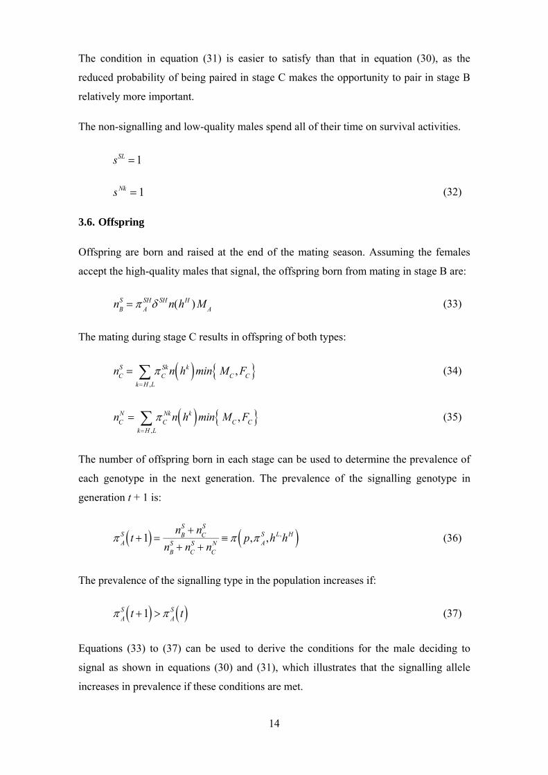
3.6. Offspring

Offspring are born and raised at the end of the mating season. Assuming the females

accept the high-quality males that signal, the offspring born from mating in stage B are:

nBS

ASH SH n(hH )M

A (33)

The mating during stage C results in offspring of both types:

nCS

kH ,L C

Skn hk min MC , FC (34)

nCN

kH ,LC

Nk n hk min MC , FC (35)

The number of offspring born in each stage can be used to determine the prevalence of

each genotype in the next generation. The prevalence of the signalling genotype in

generation t + 1 is:

AS t 1 nB

S nCS

nBS nC

S nCN p, A

S ,hL,hH

(36)

The prevalence of the signalling type in the population increases if:

AS t 1 A

S t (37)

Equations (33) to (37) can be used to derive the conditions for the male deciding to

signal as shown in equations (30) and (31), which illustrates that the signalling allele

increases in prevalence if these conditions are met.

15

3.7. Signalling equilibrium

In our specification of the model, we assume that there is a separating equilibrium

where only high-quality signalling males engage in conspicuous consumption, that

females use this signal for mate choice, and that females choose to mate only with high-

quality males in stage B. This section establishes the basis for those assumptions.

As shown by Grafen (1990a, 1990b), the core condition for the emergence of a

separating equilibrium on the basis of a signalling handicap is that the signallers of

different quality experience different costs (or benefits) to their signalling behaviour.

The low quality male must experience greater costs (or lower benefits) for the same size

signal as that produced by a high-quality signaller.

This is illustrated in Figure 1, which shows the costs and benefits of signalling for

males. The cost of a certain amount of conspicuous consumption is larger for the

low-quality male as they receive a lower wage for their labour and must sacrifice a

greater quantity of subsistence activity to match a high-quality male’s signal. The slope

of the cost curve for each quality of male is 1⁄ . The benefit of conspicuous

consumption, which is shown by the horizontal line, is the same for all males,

irrespective of their quality. The mating benefit is constant because the female decision

to mate is binary. The benefit as drawn in the chart is hypothetical, and would drop to

zero for any signal strength that a female decides to reject.

Accordingly, there is a range of signal strength that a low-quality male will not match as

the cost is above the mating benefit, while the lower cost for the high-quality male

makes signalling worthwhile. A low-quality male will set conspicuous consumption at

or below c*, while a high-quality male is prepared to signal up to a level of c’.

16

Figure 1: Costs and benefits of signalling

The threshold level that females will set can also be determined. Females set the

signal above the level at which a low-quality male is willing to signal. That is, they will

set the signal threshold above level c*. For any signal threshold up to c’, high-quality

males will be willing to signal to the observing female. If the female sets the threshold

at or below c*, both high and low-quality males would signal and the conspicuous

consumption would not be useful for mate choice. Above c’, there will be no signals.

Combining the preferred male and female strategies, it can be observed that the level of

conspicuous consumption of high-quality males will be between c* and c’ and females

will mate with males who signal in this range. However, high-quality males do not wish

to signal more than necessary and they have first mover advantage as they set the signal

before the female decides whether to mate. Therefore, high-quality males will signal at

the level (or an infinitesimal amount above) that low-quality males are indifferent about.

In other words, high-quality males will set the signal just above c*.

The females can trust this signal as it is marginally above that which a low-quality male

can copy. In this case, no-one has an incentive to deviate. If high-quality males signal at

a higher level, they reduce their survival for no mating gain, while a lower signal size

will result in no mating benefit as females cannot trust the signal. Low-quality males

will not copy the signal, as its cost exceeds its benefit to them. Females will not raise

their threshold level of acceptance as they would then miss the opportunity to mate with

17

high-quality males, while a reduction in threshold would make cheating attractive to

low-quality males.

Given = c*, we can use equation (29) to determine the proportion of time that a

high-quality male will allocate to subsistence activities. If we denote the level of

subsistence activity of a low-quality male at which he is indifferent between signalling

or not as , we can derive equation (38).

rs q

BM q

CM r qC

M

(38)

If , the relationship is:

rs 1

2 r

(39)

If the relationship is:

rs r 1ASH rs

1 r 1ASH (40)

We can then use equation (9), which describes the trade-off between subsistence

activity and conspicuous consumption, to state the relationship between survival

activities of the high-quality and low-quality types and to determine the level of

subsistence activities by the high-quality signalling type:

sSH 1 1 s hL

hH s p,

AS ,hL ,hH (41)

The level of signalling by the high-quality signalling male can be derived from

equations (39) and (40) using equation (41). Specification of a function for will allow

the values of and to be solved.

To determine which of equations (39) and (40) will apply, we must consider whether

there will be more males or females in stage C. Using equations (11) and (23),

if:

rsSH 1 1 A

SH r 2 A

SH

(42)

18

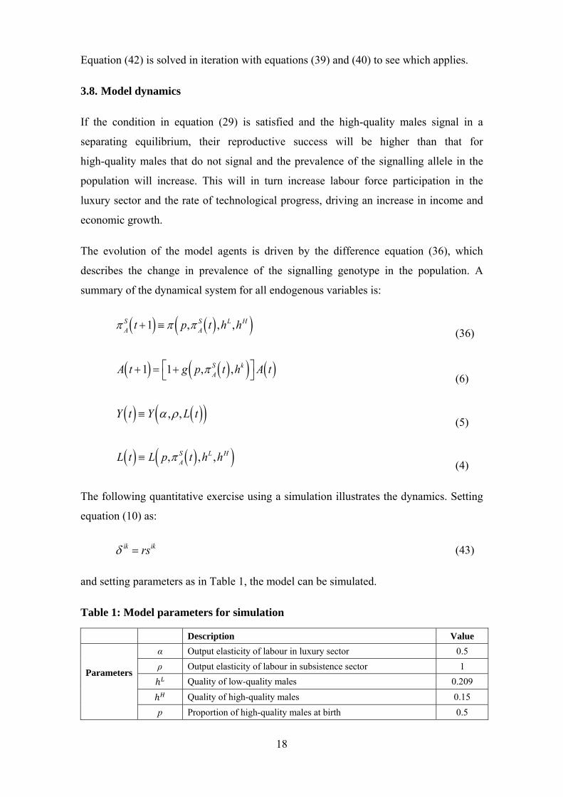
Equation (42) is solved in iteration with equations (39) and (40) to see which applies.

3.8. Model dynamics

If the condition in equation (29) is satisfied and the high-quality males signal in a

separating equilibrium, their reproductive success will be higher than that for

high-quality males that do not signal and the prevalence of the signalling allele in the

population will increase. This will in turn increase labour force participation in the

luxury sector and the rate of technological progress, driving an increase in income and

economic growth.

The evolution of the model agents is driven by the difference equation (36), which

describes the change in prevalence of the signalling genotype in the population. A

summary of the dynamical system for all endogenous variables is:

AS t 1 p,

AS t ,hL ,hH (36)

A t 1 1 g p, AS t ,hk

A t

(6)

Y t Y ,, L t (5)

L t L p,AS t ,hL ,hH (4)

The following quantitative exercise using a simulation illustrates the dynamics. Setting

equation (10) as:

ik rsik (43)

and setting parameters as in Table 1, the model can be simulated.

Table 1: Model parameters for simulation

Description Value

Parameters

α Output elasticity of labour in luxury sector 0.5

ρ Output elasticity of labour in subsistence sector 1

Quality of low-quality males 0.209

Quality of high-quality males 0.15

p Proportion of high-quality males at birth 0.5

19

Initial values

Initial prevalence of signalling allele 0.00001

A Level of technology 1

Y Income 1

g Rate of technological progress 0

X Land 1

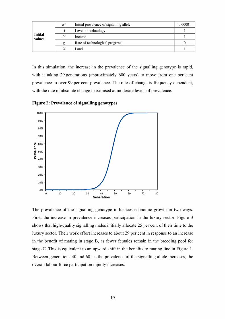
In this simulation, the increase in the prevalence of the signalling genotype is rapid,

with it taking 29 generations (approximately 600 years) to move from one per cent

prevalence to over 99 per cent prevalence. The rate of change is frequency dependent,

with the rate of absolute change maximised at moderate levels of prevalence.

Figure 2: Prevalence of signalling genotypes

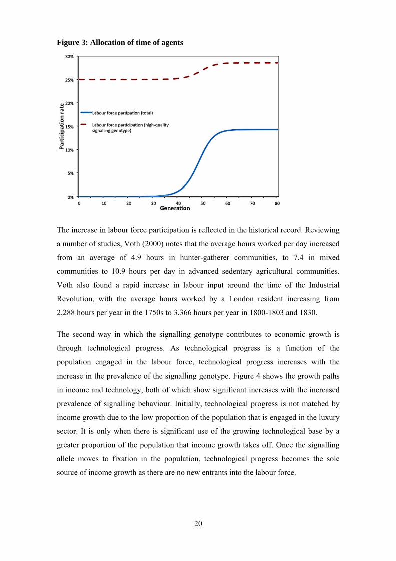
The prevalence of the signalling genotype influences economic growth in two ways.

First, the increase in prevalence increases participation in the luxury sector. Figure 3

shows that high-quality signalling males initially allocate 25 per cent of their time to the

luxury sector. Their work effort increases to about 29 per cent in response to an increase

in the benefit of mating in stage B, as fewer females remain in the breeding pool for

stage C. This is equivalent to an upward shift in the benefits to mating line in Figure 1.

Between generations 40 and 60, as the prevalence of the signalling allele increases, the

overall labour force participation rapidly increases.

20

Figure 3: Allocation of time of agents

The increase in labour force participation is reflected in the historical record. Reviewing

a number of studies, Voth (2000) notes that the average hours worked per day increased

from an average of 4.9 hours in hunter-gatherer communities, to 7.4 in mixed

communities to 10.9 hours per day in advanced sedentary agricultural communities.

Voth also found a rapid increase in labour input around the time of the Industrial

Revolution, with the average hours worked by a London resident increasing from

2,288 hours per year in the 1750s to 3,366 hours per year in 1800-1803 and 1830.

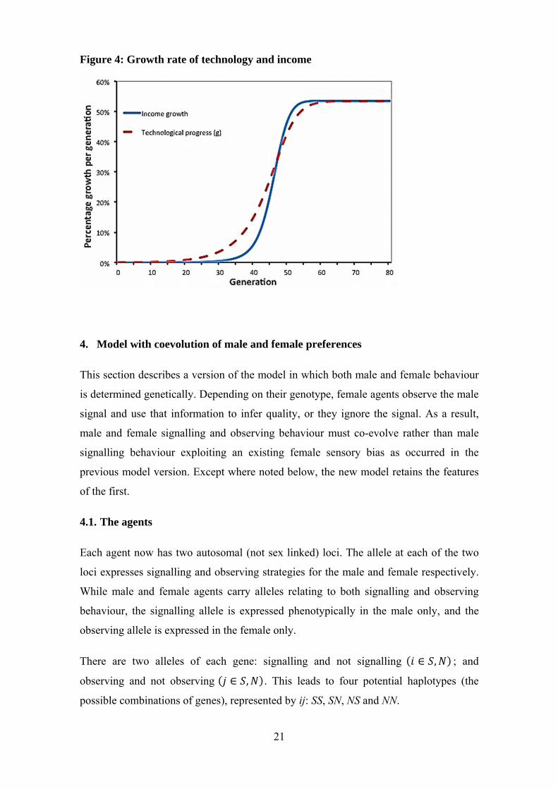
The second way in which the signalling genotype contributes to economic growth is

through technological progress. As technological progress is a function of the

population engaged in the labour force, technological progress increases with the

increase in the prevalence of the signalling genotype. Figure 4 shows the growth paths

in income and technology, both of which show significant increases with the increased

prevalence of signalling behaviour. Initially, technological progress is not matched by

income growth due to the low proportion of the population that is engaged in the luxury

sector. It is only when there is significant use of the growing technological base by a

greater proportion of the population that income growth takes off. Once the signalling

allele moves to fixation in the population, technological progress becomes the sole

source of income growth as there are no new entrants into the labour force.

21

Figure 4: Growth rate of technology and income

4. Model with coevolution of male and female preferences

This section describes a version of the model in which both male and female behaviour

is determined genetically. Depending on their genotype, female agents observe the male

signal and use that information to infer quality, or they ignore the signal. As a result,

male and female signalling and observing behaviour must co-evolve rather than male

signalling behaviour exploiting an existing female sensory bias as occurred in the

previous model version. Except where noted below, the new model retains the features

of the first.

4.1. The agents

Each agent now has two autosomal (not sex linked) loci. The allele at each of the two

loci expresses signalling and observing strategies for the male and female respectively.

While male and female agents carry alleles relating to both signalling and observing

behaviour, the signalling allele is expressed phenotypically in the male only, and the

observing allele is expressed in the female only.

There are two alleles of each gene: signalling and not signalling ∈ , ; and

observing and not observing ∈ , . This leads to four potential haplotypes (the

possible combinations of genes), represented by ij: SS, SN, NS and NN.

22

The frequency of each male phenotype by quality is denoted by ∈ , ; ∈

, ; ∈ , , while for females it is denoted by ∈ , ; ∈ , ; . denotes

the prevalence of males of genotype ij of either level of quality. Finally, the number of

males of type i is:

Ai A

ij

jS ,N (44)

while the number of females of type j is:

Aj

Aij

iS ,N (45)

The utility function of a male is the number of children they father. Similarly, the utility

function of a female is the number of children they bear, which is equal to the quality of

the male with whom they mate, as in equations (1) and (2). Children inherit the allele at

each locus with equal probability from each parent.

4.2. The economy

The economy in the two-locus model is the same as in the single locus model. The one

substantive difference is that there are more male genotypes as males also carry the gene

that expresses female observing behaviour. Accordingly, the number of efficiency units

of labour in the subsistence and luxury sectors are:

S t M t Aijksijkhk

jS ,N

iS ,N

kH ,L (46)

L t M t hH ASjH

jS ,N (1 sSjH

jS ,N ) (47)

4.3. The mating season

As for the single-locus model, each generation lives for one mating season, which

comprises three stages. Equal numbers of males and females are born, so before

signalling and mortality, the number of each sex is equal.

Males signal subject to a budget constraint and then experience mortality based on the

level of subsistence activities. The budget constraint and probability of survival are:

23

cijk whk 1 sSjk (48)

ik rsijk

sik rsijk 0

ssik rsijk 0 (49)

0 0 r 1

As the probability of survival of a male is not affected by the observing allele at locus j,

the j subscript is dropped.

After pre-breeding mortality in stage A, the number of males who are available to mate

in stage B is:

M B Aijk ik

jS ,N

iS ,N

kH ,L M A (50)

The prevalence of surviving males of each type is:

Bijk

Aijk ik M

A

MB

(51)

i S , N j S , N k H , L

The number of females does not change between stage A and B, as there is no female

mortality.

A male always agrees to mate with the female he is matched with, as there is no cost to

mating for males. The probability of being matched in stage B is one for a male, as male

mortality ensures that there are more males than females. The probability of a female

being matched with a male is:

qBF A

ijk ik

jS ,N

iS ,N

kH ,L (52)

If a female is paired in stage B, a female of the observing phenotype (SS or NS)

observes the signal of the male and uses that signal to determine whether she will mate

with the male. If she does choose to mate, the female exits the mating pool. If she is of

the non-observing phenotype (SN or NN), she will mate with the male regardless of his

signal or quality. Accordingly, non-observing females are only present in stage C if they

are not paired in stage B.

24

The number of males and the ratio of types of males do not change between stages B

and C.

Cijk B

ijk (53)

The number of females available for mating in stage C decreases by the number who

mate in stage B. Females exit the breeding pool if they are a observing genotype and are

matched with a high-quality signalling male, or, if they are not a observing genotype

and are matched at all.

FC

BS 1 q

BF

BSjH

jS ,N

BN 1 q

BF

F

B (54)

The proportion of females of each phenotype present in stage C is:

CS

BS 1 q

BF

BSjH

jS ,N

FB

FC

(55)

CN

BN 1 q

BF F

B

FC

(56)

It is possible for males and females to be unmatched in stage C (as in equations (18) and

(19)). In stage C, males and females will mate with whoever they are matched, as

females will have no further opportunities to mate. Offspring from the mating in stages

B and C form the next generation.

4.4. Female optimisation

A female carrying the observing allele (haplotype SS and NS) will mate in stage B if the

benefit exceeds the expected benefit of waiting. The future benefit is a function of the

probability that she will be matched to a male in stage C and the expected quality of that

male. She will mate with the male of quality hk in stage B if:

n hk qCF C

ijH n hH CijLn hL

jS ,N

iS ,N (57)

25

This will only be satisfied for a low-quality male if:

n hL q

CF

CijH

jS ,N

iS ,N

1 qCF

CijL

jS ,N

iS ,N

n hH (58)

As for the single-locus model and the similar condition stated in equation (21), we

assume that equation (58) is not satisfied. This is a weaker assumption in the current

model due to paired, non-observing females exiting the breeding pool with certainty in

stage B, making it unlikely that there will be excess females in stage C. As in the earlier

model, the decision of the female is binary, based on the threshold level of conspicuous

consumption that is given in equation (22).

4.5. Male optimisation

The male’s utility (fitness) function is:

u

tSjk Sk c

tijk B

S BN qB

M qCM n hk (59)

u

tNk Sk

BN q

BM q

CM n hk (60)

Substituting equation (9) into equations (59) and (60), a male of generation t faces the

following optimisation problem:

stSjk argmax Sk wthk 1 st

Sjk BS B

N qBM qC

M n hk

(61)

stNjk argmax NkqC

M n hk (62)

Solving equation (61) for the signalling genotype gives:

sSk B

S BN qB

M qCM Sk wth

k sqBM (63)

As before, the male invests in conspicuous consumption until the marginal gain in

fitness through additional mating opportunity is equal to the marginal loss through

decreased survival.

26

Since the female decision is binary, a high-quality signalling male will signal where the

following condition holds:

q

BM q

CM SH

AN q

CM NH

(64)


2 SH NH

AN 1 (65)

This condition reflects that high-quality, signalling males mate with certainty in both

periods, while all other male phenotypes mate in stage B if they are paired with a

non-choosy female, and with certainty in stage C. If most females are of the observing

genotype, a male will be willing to sacrifice only a small probability of survival to

signal to females.


1 q

CM SH

AN q

CM NH (66)

The condition in equation (66) is easier to satisfy than that in equation (65). This is

because the reduced probability of being paired in stage C makes the opportunity to pair

in stage B relatively more important.

For the non-signalling and low-quality phenotypes, they spend all of their time on

survival activities.

stNjk 1

stSjL 1 (67)

27

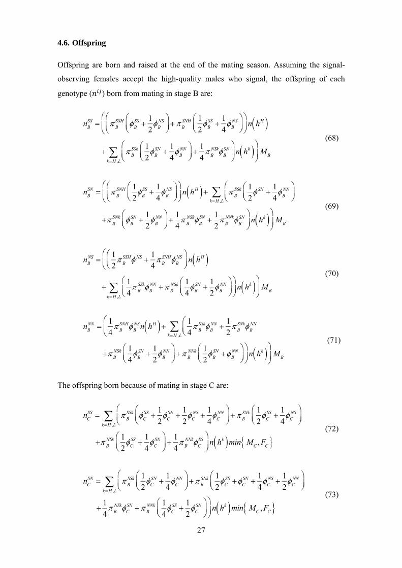
4.6. Offspring

Offspring are born and raised at the end of the mating season. Assuming the signal-

observing females accept the high-quality males who signal, the offspring of each

genotype ( ) born from mating in stage B are:

nBSS

BSSH

BSS

1

2

BNS

BSNH 1

2

BSS

1

4

BNS

n hH

kH ,L

BSSk 1

2

BSN

1

4

BNN

1

4

BNSk

BSN

n hk

M

B

(68)

nBSN

BSNH 1

2

BSS

1

4

BNS

n hH

BSSk 1

2 SN

1

4

BNN

kH ,L

BSNk

BSN

1

2

BNN

1

4

BNSk

BSN

1

2

BNNk

BSN

n hk

M

B

(69)

nBNS

12

BSSH NS

14

BSNH

BNS

n hH

kH ,L

1

4

BSSk

BNN

BNSk 1

4

BSN

1

2

BNN

n hk

M

B

(70)

nBNN

1

4

BSNH

BNS n hH 1

4

BSSk

BNN

1

2

BSNk

BNN

kH ,L

BNSk 1

4

BSN

1

2

BNN

BNNk 1

2

BSN

BNN

n hk

M

B

(71)

The offspring born because of mating in stage C are:

nCSS

kH ,L B

SSk CSS

1

2C

SN 1

2C

NS 1

4C

NN

B

SNk 1

2C

SS 1

4C

NS

BNSk 1

2

CSS

1

4

CSN

1

4

BNNk

CSS

n hk min M

C, F

C (72)

nCSN

kH ,L B

SSk 1

2C

SN 1

4C

NN

B

SNk 1

2C

SS CSN

1

4C

NS 1

2C

NN

1

4

BNSk

CSN

BNNk 1

4

CSS

1

2

CSN

n hk min M

C, F

C (73)

28

nCNS

kH ,L

BSSk 1

2

CNS

1

4

CNN

1

4

BSNk

CNS

BNSk 1

2

CSS

1

4

CSN

CNS

1

2

CNN

BNNk 1

4

CSS

1

2

CNS

n hk min M

C, F

C

(74)

nCNN

kH ,L

1

4 B

SSkCNN B

SNk 1

4C

NS 1

2C

NN

B

NSk 1

4C

SN 1

2C

NN

BNNk 1

4

CSS

1

2

CSN

1

2

CNS

CNN

n hk min M

C, F

C (75)

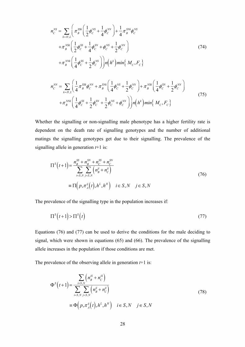
Whether the signalling or non-signalling male phenotype has a higher fertility rate is

dependent on the death rate of signalling genotypes and the number of additional

matings the signalling genotypes get due to their signalling. The prevalence of the

signalling allele in generation t+1 is:

S t 1 nBSS n

BSN n

CSS n

CSN

nBij n

Cij

jS ,N

iS ,N

p,Aij t ,hL ,hH i S, N j S, N

(76)

The prevalence of the signalling type in the population increases if:

S t 1 S t (77)

Equations (76) and (77) can be used to derive the conditions for the male deciding to

signal, which were shown in equations (65) and (66). The prevalence of the signalling

allele increases in the population if those conditions are met.

The prevalence of the observing allele in generation t+1 is:

S t 1 n

BiS n

CiS

iS ,N

nBij n

Cij

jS ,N

iS ,N

p, Aij t ,hL ,hH iS , N j S , N

(78)

29

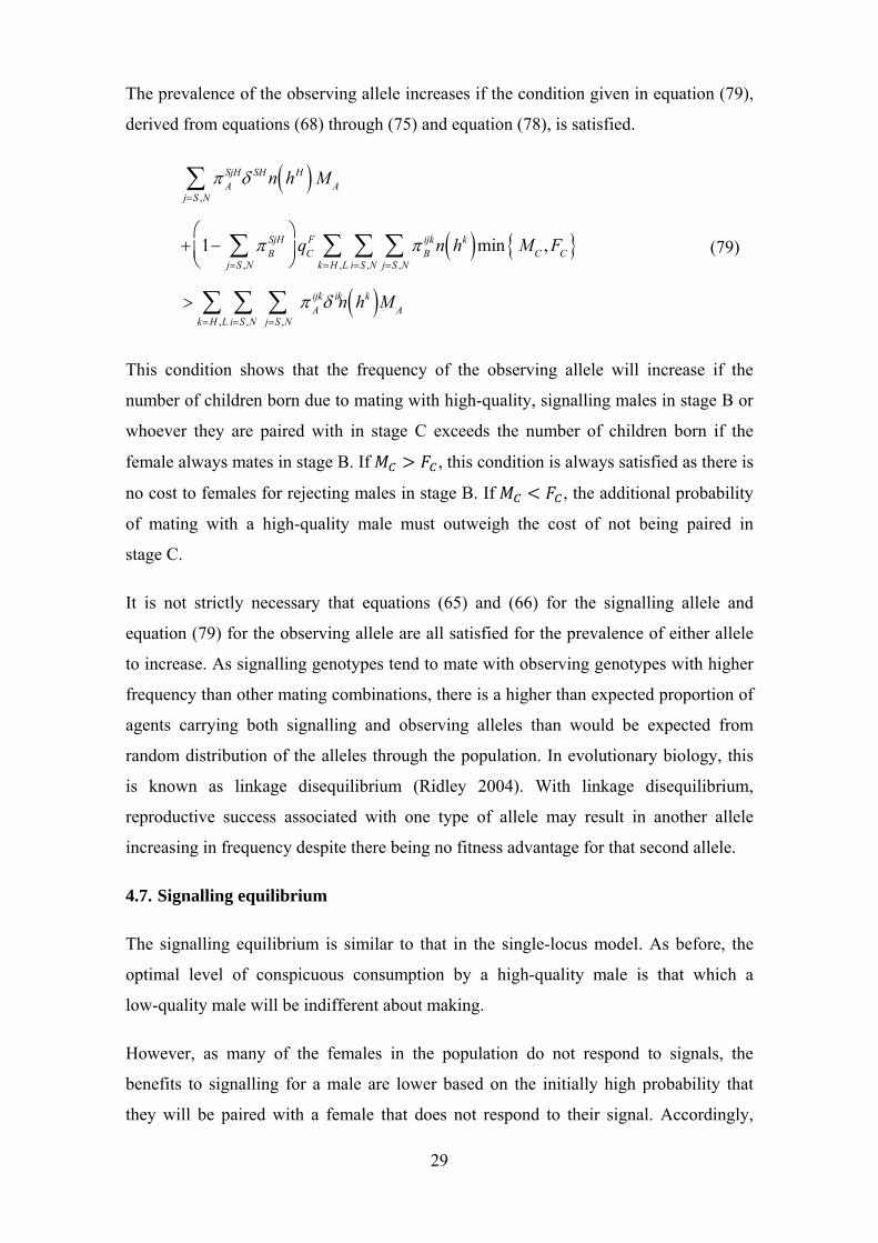
The prevalence of the observing allele increases if the condition given in equation (79),

derived from equations (68) through (75) and equation (78), is satisfied.

ASjH

jS ,N SH n hH M

A

1 BSjH

jS ,N

q

CF

Bijkn hk

jS ,N

iS ,N

kH ,L min M

C, F

C

Aijk ikn hk

jS ,N

iS ,N M

AkH ,L

(79)

This condition shows that the frequency of the observing allele will increase if the

number of children born due to mating with high-quality, signalling males in stage B or

whoever they are paired with in stage C exceeds the number of children born if the

female always mates in stage B. If , this condition is always satisfied as there is

no cost to females for rejecting males in stage B. If , the additional probability

of mating with a high-quality male must outweigh the cost of not being paired in

stage C.

It is not strictly necessary that equations (65) and (66) for the signalling allele and

equation (79) for the observing allele are all satisfied for the prevalence of either allele

to increase. As signalling genotypes tend to mate with observing genotypes with higher

frequency than other mating combinations, there is a higher than expected proportion of

agents carrying both signalling and observing alleles than would be expected from

random distribution of the alleles through the population. In evolutionary biology, this

is known as linkage disequilibrium (Ridley 2004). With linkage disequilibrium,

reproductive success associated with one type of allele may result in another allele

increasing in frequency despite there being no fitness advantage for that second allele.

4.7. Signalling equilibrium

The signalling equilibrium is similar to that in the single-locus model. As before, the

optimal level of conspicuous consumption by a high-quality male is that which a

low-quality male will be indifferent about making.

However, as many of the females in the population do not respond to signals, the

benefits to signalling for a male are lower based on the initially high probability that

they will be paired with a female that does not respond to their signal. Accordingly,

30

high-quality signalling males tend to signal through a lower level of conspicuous

consumption until the prevalence of observing females increases.

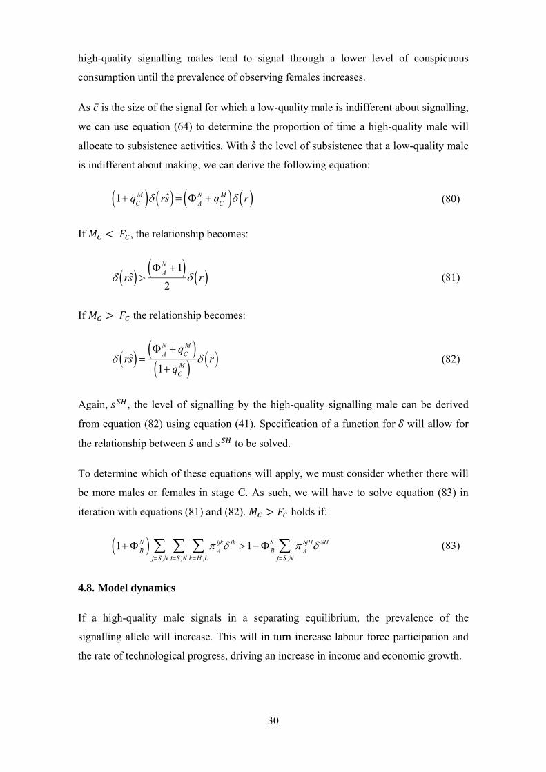
As is the size of the signal for which a low-quality male is indifferent about signalling,

we can use equation (64) to determine the proportion of time a high-quality male will

allocate to subsistence activities. With the level of subsistence that a low-quality male

is indifferent about making, we can derive the following equation:

1 q

CM rs

AN q

CM r

(80)

If , the relationship becomes:

rs

AN 1 2

r (81)

If the relationship becomes:

rs A

N qCM

1 qCM r (82)

Again, , the level of signalling by the high-quality signalling male can be derived

from equation (82) using equation (41). Specification of a function for will allow for

the relationship between and to be solved.

To determine which of these equations will apply, we must consider whether there will

be more males or females in stage C. As such, we will have to solve equation (83) in

iteration with equations (81) and (82). holds if:

1BN A

ijk ik

kH ,L

iS ,N

jS ,N 1B

S ASjH

jS ,N SH

(83)

4.8. Model dynamics

If a high-quality male signals in a separating equilibrium, the prevalence of the

signalling allele will increase. This will in turn increase labour force participation and

the rate of technological progress, driving an increase in income and economic growth.

31

The dynamics of the evolution of the model agents is determined by the difference

equations (76) and (78). A summary of the dynamical system for all endogenous

variables is:

Aij t 1 p,

Aij t ,hL ,hH iS , N j S, N

(76)

Aij t 1 A

ij t 1 iS, N j S, N (78)

A t 1 1 g p, ASj t , iS t ,hk

A t i S , N ; j S , N

(6)

Y t Y ,, L t (5)

L t L p,ASj t , iS t ,hL ,hH iS , N ; j S, N

(47)

Again, the model is simulated using equation (43) for survival probability, and setting

the parameters as in Table 2.

Table 2: Model parameters for simulation

Description Value

Parameters

Output elasticity of labour 0.5

ρ Output elasticity of labour in subsistence sector 1

Quality of low-quality males 0.209

Quality of high-quality males 0.15

p Proportion of high-quality males at birth 0.5

Initial values

Initial prevalence of signalling allele (S) 0.01

Initial prevalence of observing allele (S) 0.01

A Level of technology 1

Y Income 1

g Rate of technological progress 0

X Land 1

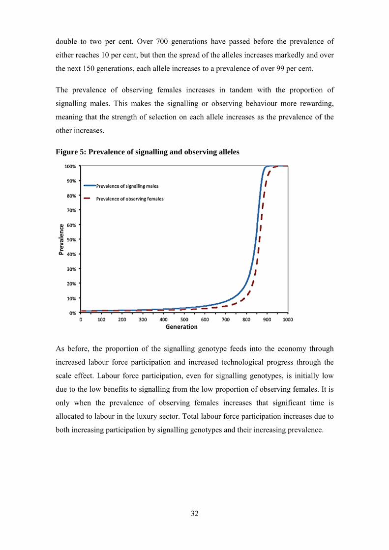
Figure 5 shows the proportion of signalling and observing alleles in the population. The

increase in prevalence of the signalling allele is significantly slower than that in the first

model in which all females have a genetic predisposition to observe male conspicuous

consumption. It takes approximately 350 generations for the prevalence of the

signalling allele and almost 500 generations for the prevalence of the observing allele to

32

double to two per cent. Over 700 generations have passed before the prevalence of

either reaches 10 per cent, but then the spread of the alleles increases markedly and over

the next 150 generations, each allele increases to a prevalence of over 99 per cent.

The prevalence of observing females increases in tandem with the proportion of

signalling males. This makes the signalling or observing behaviour more rewarding,

meaning that the strength of selection on each allele increases as the prevalence of the

other increases.

Figure 5: Prevalence of signalling and observing alleles

As before, the proportion of the signalling genotype feeds into the economy through

increased labour force participation and increased technological progress through the

scale effect. Labour force participation, even for signalling genotypes, is initially low

due to the low benefits to signalling from the low proportion of observing females. It is

only when the prevalence of observing females increases that significant time is

allocated to labour in the luxury sector. Total labour force participation increases due to

both increasing participation by signalling genotypes and their increasing prevalence.

33

Figure 6: Allocation of time of agents

Figure 7 shows the growth paths in technology and income. For the first 500

generations, the rate of technological progress exceeds income growth due to the low

proportion of the population that is engaged in the luxury sector. It is only when there is

significant use of the growing technological base by a greater proportion of the

population that income growth takes off. Once the signalling allele moves to fixation in

the population, technological progress becomes the sole source of income growth, as

there are no new entrants into the labour force.

Figure 7: Growth rate of technology and income

34

5. Discussion

The two models presented above provide a basis for the hypothesis that the male

signalling behaviour necessary to attract potential mates underpins modern levels of

economic growth. As females prefer males who conspicuously consume, an increasing

proportion of males engage in innovation, labour and other productive activities in order

to engage in conspicuous consumption. These activities contribute to technological

progress and economic growth.

Which of the two versions of the model is more realistic is unclear. Positive responses

to expensive watches and cars, to which females have had limited exposure in our

evolutionary history, suggest significant flexibility over short timeframes in human

perception of what is a reliable signal. Conversely, anthropological evidence and the

ubiquity of conspicuous consumption in human society suggest a deep evolutionary

basis to this trait, which may have developed over significant time (Sundie et al. 2011).

The core condition for a handicap to be an honest signal is different costs (or benefits)

of signalling between high and low-quality signallers. In our model, the difference in

costs to signalling arises from the difference in wages that each high and low-quality

male can earn in the luxury sector of the economy, which produces conspicuous

consumption goods. Even if there was no such wage difference, the necessary condition

for existence of the handicap as an honest signal could have been met through

alternative means. The models could be reframed so that high and low-quality males

experienced different costs to allocating time away from subsistence activities, with the

survival probability for low-quality males declining faster. By amending the survival

equation (10) to also be a function of quality and stating the second order equation as a

strict inequality, as shown in equation (84), the condition for the handicap principle

would hold even in the absence of a wage differential. The increased survival cost faced

by a low-quality male would allow a separating equilibrium to exist.

ik rsik hk

sik rsik hk 0

ssik rsik hk 0 (84)

0 0 r 1 1

35

If it were assumed that the “quality” trait affected multiple areas, including survival

probability and labour efficiency, the condition for the handicap would be met in

multiple dimensions.

The two models differ greatly in the speed at which the conspicuous consumption

behaviour spreads through the population. The first model produces significant changes

in economic behaviour within one to two hundred years, resulting a rapid take-off in

economic growth, similar to that which occurred around the time of the Industrial

Revolution. The second model gives rise to longer-term trends in economic growth,

which, when combined with population growth, may not result in observable per capita

income changes for long periods.

In both models, sexual selection does not affect the quality of the agents. Quality is

allocated randomly at birth, which made the model tractable for an analysis of the

handicap principle. If quality were genetically transmitted between generations,

selection of high-quality individuals would tend to drive the genes associated with high

quality to fixation, at which point female choice would become obsolete. A more

realistic but complicated scenario would be to introduce multiple genes associated with

quality and allow mutations of these genes. This would allow selection by females to

remain important, while allowing qualitative population changes to occur. We consider

that this scenario would be more representative of the human evolutionary history, with

the propensity for conspicuous consumption and qualitative traits both being selected

for in the population.

In addition to being a signal of quality, conspicuous consumption is a signal of

underlying wealth, which is likely to be of value to a female in itself. Female interest in

wealth accumulation is likely to play a significant role in the evolution of a preference

for conspicuous consumption. In the models in this paper, agents do not accumulate

wealth as there is no capital and there is no transmission of resources from males to

females. The ability to accumulate wealth may change the inherent trade-offs between

quality and signalling ability, particularly if resources can be transmitted to children.

One omission is the positive effect on survival of the activities undertaken to support

conspicuous consumption. The labour and innovation of previous centuries has not only

improved the methods to acquire resources for conspicuous consumption, but has also

affected basic survival probability. In modern developed-country economies, survival to

36

adulthood is likely with probability above 99 per cent (Department of Economic and

Social Affairs 2011). Since conspicuous consumption imposes no real cost on survival

in modern contexts, everyone engages in conspicuous consumption to the extent their

wealth permits. This might be incorporated into the model through allowing some

portion of returns to conspicuous consumption to eventually be used to improve

survival probability or by providing for spill-over of technological progress into the

subsistence sector.

This is not to say, however, that conspicuous consumption can have no survival cost

today. Conspicuous consumption also occurs in poor societies, often at significant cost

to the signallers. It has been theorised that conspicuous consumption is more important

in poor societies than in societies with higher income as in developed countries people

can signal through career, qualifications or other costly methods of demonstrating

quality (Moav & Neeman 2012).

References

Andersson, M 1994, Sexual Selection, Princeton University Press, Princeton.

Basolo, AL 1990, ‘Female Preference Predates the Evolution of the Sword in Swordtail Fish’, Science, vol. 250, no. 4982, pp. 808–810.

Bateman, AJ 1948, ‘Intra-sexual selection in Drosophila’, Heredity, vol. 2, no. 3, pp. 349–368.

Borgerhoff Mulder, M 1990, ‘Kipsigis Women’s Preferences for Wealthy Men: Evidence for Female Choice in Mammals’, Behavioral Ecology and Sociobiology, vol. 27, no. 4, pp. 255–264.

Brown, GR, Laland, KN & Mulder, MB 2009, ‘Bateman’s principles and human sex roles’, Trends in Ecology and Evolution, vol. 24, no. 6, pp. 297–304.

Clark, G 2007, A Farewell to Alms: A Brief Economic History of the World, Princeton University Press, Princeton and Oxford.

Cronk, L 1991, ‘Wealth, Status, and Reproductive Success among the Mukogodo of Kenya’, American Anthropologist, vol. 93, no. 2, pp. 345–360.

Darwin, C 1871, The Descent of Man and Selection in Relation to Sex, John Murray, London.

Department of Economic and Social Affairs 2011, 2009-10 Demographic Yearbook, United Nations, New York.

37

Fisher, RA 1930, The Genetical Theory of Natural Selection, Clarendon Press, Oxford.

De Fraja, G 2009, ‘The origin of utility: Sexual selection and conspicuous consumption’, Journal of Economic Behavior & Organization, vol. 72, no. 1, pp. 51–69.

Frank, RH 1999, Luxury Fever, The Free Press, New York.

Galor, O & Michalopoulos, S 2011, ‘Evolution and the Growth Process: Natural Selection of Entrepreneurial Traits’, Journal of Economic Theory.

Galor, O & Moav, O 2002, ‘Natural Selection and the Origin of Economic Growth’, Quarterly Journal of Economics, vol. 117, no. 4, pp. 1133–1191.

Grafen, A 1990a, ‘Biological signals as handicaps’, Journal of Theoretical Biology, vol. 144, no. 4, pp. 517–546.

Grafen, A 1990b, ‘Sexual selection unhandicapped by the fisher process’, Journal of Theoretical Biology, vol. 144, no. 4, pp. 473–516.

Griskevicius, V, Tybur, JM, Sundie, JM, Cialdini, RB, Miller, GF & Kenrick, DT 2007, ‘Blatant benevolence and conspicuous consumption: When romantic motives elicit strategic costly signals.’, Journal of Personality and Social Psychology, vol. 93, no. 1, pp. 85–102.

Hopcroft, RL 2006, ‘Sex, status, and reproductive success in the contemporary United States’, Evolution and Human Behaviour, vol. 27, no. 2, pp. 104–120.

Kremer, M 1993, ‘Population Growth and Technological Change: One Million B.C. to 1990’, Quarterly Journal of Economics, vol. 108, no. 3, pp. 681–716.

Maynard Smith, J 1978, The Evolution of Sex, Cambridge University Press, Cambridge.

Miller, GF 1999, ‘Waste is good’, Prospect, no. 38.

Miller, GF 2001, The Mating Mind: How Sexual Choice Shaped the Evolution of Human Nature, Anchor, New York.

Moav, O & Neeman, Z 2012, ‘Saving Rates and Poverty: The Role of Conspicuous Consumption and Human Capital’, The Economic Journal, p. no.

Mulder, MB 1987, ‘On Cultural and Reproductive Success: Kipsigis Evidence’, American Anthropologist, vol. 89, no. 3, pp. 617–634.

R Development Core Team 2010, R: A Language and Environment for Statistical Computing, R Foundation for Statistical Computing, Vienna, Austria.

Ridley, M 2004, Evolution, Blackwell Publishing, Malden.

Romer, PM 1990, ‘Endogenous Technological Change’, Journal of Political Economy, vol. 98, no. 5, pp. S71–S102.

Ryan, MJ 1990, ‘Sexual selection, sensory systems and sensory exploitation’, Oxford Surveys in Evolutionary Biology, vol. 7, pp. 157–195.

38

Ryan, MJ 1998, ‘Sexual Selection, Receiver Biases, and the Evolution of Sex Differences’, Science, vol. 281, no. 5385, pp. 1999–2003.

Saad, G 2007, The Evolutionary Bases of Consumption, Lawrence Erlbaum Associates, Mahwah.

Spence, M 1973, ‘Job Market Signaling’, The Quarterly Journal of Economics, vol. 87, no. 3, pp. 355–374.

Sundie, JM, Kenrick, DT, Griskevicius, V, Tybur, JM, Vohs, KD & Beal, DJ 2011, ‘Peacocks, Porsches, and Thorstein Veblen: Conspicuous Consumption as a Sexual Signaling System’, Journal of Personality and Social Psychology, vol. 100, no. 4, pp. 664–680.

Trivers, RL 1972, ‘Parental investment and sexual selection’, in, Sexual Selection and the Descent of Man 1871-1971, Aldine Publishing Company, Chicago.

Veblen, T 1899, The Theory of the Leisure Class, Macmillan, New York, London.

Voth, H-J 2000, Time and Work in England 1750-1830, Oxford University Press, Oxford.

Wade, MJ 1979, ‘Sexual Selection and Variance in Reproductive Success’, The American Naturalist, vol. 114, no. 5, pp. 742–747.

Wade, MJ & Shuster, SM 2004, ‘Estimating the Strength of Sexual Selection From Y‐Chromosome And Mitochondrial DNA Diversity’, Evolution, vol. 58, no. 7, pp. 1613–1616.

Zahavi, A 1975, ‘Mate selection--A selection for a handicap’, Journal of Theoretical Biology, vol. 53, no. 1, pp. 205–214.

Zak, PJ & Park, KW 2002, ‘Population Genetics and Economic Growth’, Journal of Bioeconomics, vol. 4, no. 1, pp. 1–38.

39

Appendix A: R code for simulations

[For the reviewer only – not for publication]

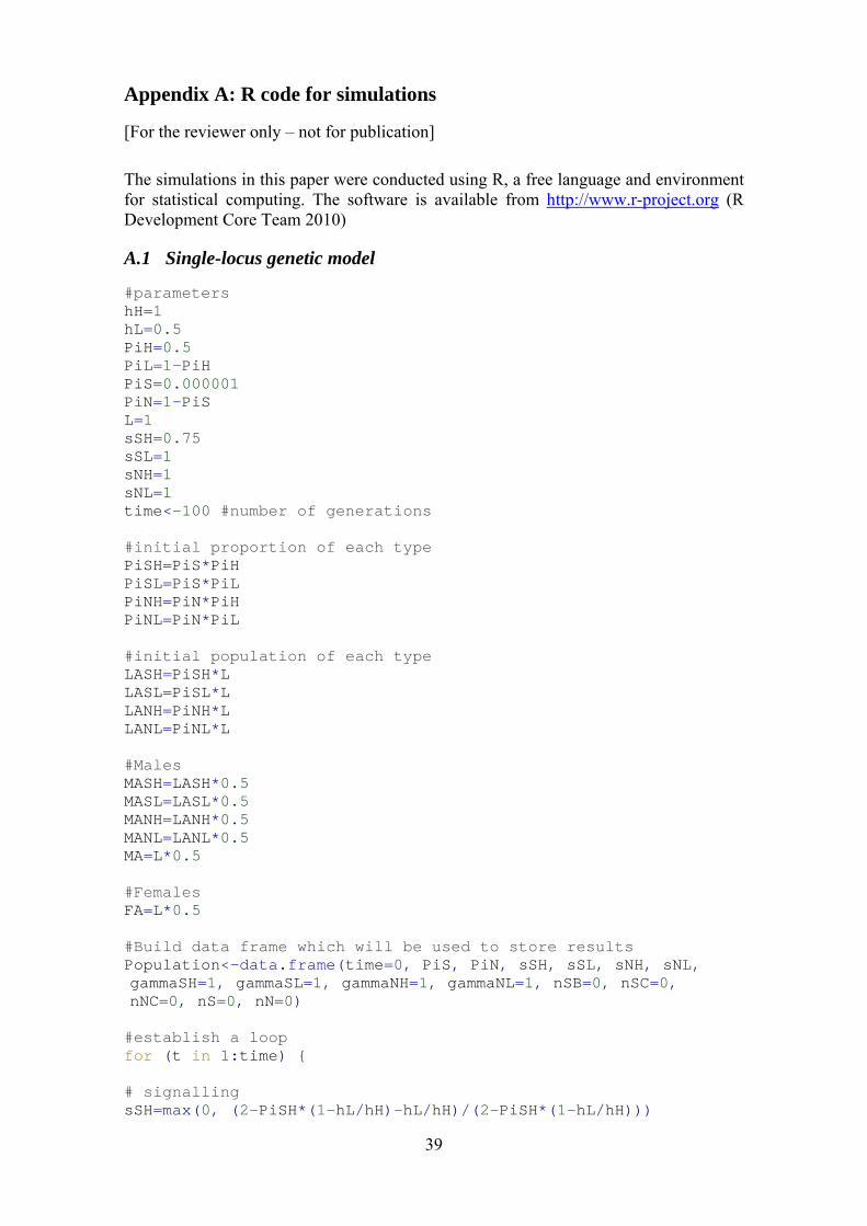
The simulations in this paper were conducted using R, a free language and environment for statistical computing. The software is available from http://www.r-project.org (R Development Core Team 2010)

A.1 Single-locus genetic model

#parameters hH=1 hL=0.5 PiH=0.5 PiL=1-PiH PiS=0.000001 PiN=1-PiS L=1 sSH=0.75 sSL=1 sNH=1 sNL=1 time<-100 #number of generations #initial proportion of each type PiSH=PiS*PiH PiSL=PiS*PiL PiNH=PiN*PiH PiNL=PiN*PiL #initial population of each type LASH=PiSH*L LASL=PiSL*L LANH=PiNH*L LANL=PiNL*L #Males MASH=LASH*0.5 MASL=LASL*0.5 MANH=LANH*0.5 MANL=LANL*0.5 MA=L*0.5 #Females FA=L*0.5 #Build data frame which will be used to store results Population<-data.frame(time=0, PiS, PiN, sSH, sSL, sNH, sNL, gammaSH=1, gammaSL=1, gammaNH=1, gammaNL=1, nSB=0, nSC=0, nNC=0, nS=0, nN=0) #establish a loop for (t in 1:time) { # signalling sSH=max(0, (2-PiSH*(1-hL/hH)-hL/hH)/(2-PiSH*(1-hL/hH)))

40

sSL=1 sNH=1 sNL=1 #survival gammaSH=sSH gammaSL=sSL gammaNH=sNH gammaNL=sNL #surviving males MBSH=MASH*gammaSH MBSL=MASL*gammaSL MBNH=MANH*gammaNH MBNL=MANL*gammaNL MB=MBSH+MBSL+MBNH+MBNL #proportion surviving by type PiSH=MBSH/MB PiSL=MBSL/MB PiNH=MBNH/MB PiNL=MBNL/MB #number of children in Stage B nSB=MBSH*hH #Number of females available in Stage C FC=max(0,FA-MBSH) #number of children in Stage C #note - always more males than females in Stage C under parameters chosen nSC=(PiSH*hH+PiSL*hL)*FC nNC=(PiNH*hH+PiNL*hL)*FC #total number of children of each type nS=nSB+nSC nN=nNC n=nS+nN #proportion of each type of children (next generation) PiS=nS/n PiN=nN/n #population by type and quality next generation (currently written to ignore population change) PiSH=PiS*PiH PiSL=PiS*PiL PiNH=PiN*PiH PiNL=PiN*PiL LA=1 LASH=PiSH*LA LASL=PiSL*LA LANH=PiNH*LA LANL=PiNL*LA MA=LA*0.5 FA=LA*0.5

41

MASH=PiSH*MA MASL=PiSL*MA MANH=PiNH*MA MANL=PiNL*MA #Bind the new generation of results to the data frame Population<-rbind(Population, c(t, PiS, PiN, sSH, sSL, sNH, sNL, gammaSH, gammaSL, gammaNH, gammaNL, nSB, nSC, nNC, nS, nN)) #close loop } Population

A.2 Two-locus genetic model

#parameters hH=1 hL=0.5 PiH=0.5 PiL=1-PiH PiSj=0.01 PiNj=1-PiSj PhiiS=0.01 PhiiN=1-PhiiS LA=1 sSjH=1 sSjL=1 sNjH=1 sNjL=1 time<-1000 #number of generations #initial proportion of each type of male PiSS=PiSj*PhiiS PiSN=PiSj*PhiiN PiNS=PiNj*PhiiS PiNN=PiNj*PhiiN #initial proportion of each type of female PhiSS=PhiiS*PiSj PhiSN=PhiiN*PiSj PhiNS=PhiiS*PiNj PhiNN=PhiiN*PiNj #Build data frame which will be used to store results Population<-data.frame(time=0, PiSj, PiNj, PhiiS, PhiiN, sSjH, sSjL, sNjH, sNjL, gammaSjH=1, gammaSjL=1, gammaNjH=1, gammaNjL=1, nSS=0, nSN=0, nNS=0, nNN=0) #establish a loop for (t in 1:time) { #population by type and quality next generation (currently written to ignore population change) PiSSH=PiSS*PiH PiSSL=PiSS*PiL

42

PiSNH=PiSN*PiH PiSNL=PiSN*PiL PiNSH=PiNS*PiH PiNSL=PiNS*PiL PiNNH=PiNN*PiH PiNNL=PiNN*PiL PiSjH=PiSj*PiH PiSjL=PiSj*PiL PiNjH=PiNj*PiH PiNjL=PiNj*PiL #as proportions of males and females equal before signalling PhiSS=PiSS PhiSN=PiSN PhiNS=PiNS PhiNN=PiNN #population level MA=LA*0.5 FA=LA*0.5 #number of males MASSH=PiSSH*MA MASNH=PiSNH*MA MASSL=PiSSL*MA MASNL=PiSNL*MA MANSH=PiNSH*MA MANNH=PiNNH*MA MANSL=PiNSL*MA MANNL=PiNNL*MA #number of females FASS=PhiSS*FA FASN=PhiSN*FA FANS=PhiNS*FA FANN=PhiNN*FA # signalling - determine signalling for male shortage in Stage C, check male/female ratio and amend if required sSjHtest1=1-(PhiiS/2)*(hL/hH) sSjHtest2=(1+PhiiS*(1-PiSjH)*(1-hL/hH))/(1+PhiiS*(1-PiSjH*(1-hL/hH))) sSjH=max(0, if(sSjHtest1<PiSjH-PhiiN*(1-PiSjH)/(2*PiSjH)) sSjHtest1 else sSjHtest2) sSjL=1 sNjH=1 sNjL=1 #test variable for whether Mc>Fc #survival gammaSjH=sSjH gammaSjL=sSjL gammaNjH=sNjH gammaNjL=sNjL

43

#surviving males MBSSH=MASSH*gammaSjH MBSNH=MASNH*gammaSjH MBSSL=MASSL*gammaSjL MBSNL=MASNL*gammaSjL MBNSH=MANSH*gammaNjH MBNNH=MANNH*gammaNjH MBNSL=MANSL*gammaNjL MBNNL=MANNL*gammaNjL MB=MBSSH+MBSNH+MBSSL+MBSNL+MBNSH+MBNNH+MBNSL+MBNNL #proportion surviving by type PiSSH=MBSSH/MB PiSNH=MBSNH/MB PiSjH=PiSSH+PiSNH PiSSL=MBSSL/MB PiSNL=MBSNL/MB PiNSH=MBNSH/MB PiNNH=MBNNH/MB PiNSL=MBNSL/MB PiNNL=MBNNL/MB #proportion of males to females in Stage B qFB=MB/FA #number of children in Stage B nSSB=((PiSSH*(PhiSS+0.5*PhiNS)+PiSNH*(0.5*PhiSS+0.25*PhiNS))*hH+(PiSSH*(0.5*PhiSN+0.25*PhiNN)+0.25*PiNSH*PhiSN)*hH+(PiSSL*(0.5*PhiSN+0.25*PhiNN)+0.25*PiNSL*PhiSN)*hL)*MB nSNB=(PiSNH*(0.5*PhiSS+0.25*PhiNS)*hH+(PiSSH*(0.5*PhiSN+0.25*PhiNN)+PiSNH*(PhiSN+0.5*PhiNN)+0.25*PiNSH*PhiSN+0.5*PiNNH*PhiSN)*hH+(PiSSL*(0.5*PhiSN+0.25*PhiNN)+PiSNL*(PhiSN+0.5*PhiNN)+0.25*PiNSL*PhiSN+0.5*PiNNL*PhiSN)*hL)*MB nNSB=((0.5*PiSSH*PhiNS+0.25*PiSNH*PhiNS)*hH+(0.25*PiSSH*PhiNN+PiNSH*(0.25*PhiSN+0.5*PhiNN))*hH+(0.25*PiSSL*PhiNN+PiNSL*(0.25*PhiSN+0.5*PhiNN))*hL)*MB nNNB=(0.25*PiSNH*PhiNS*hH+(0.25*PiSSH*PhiNN+0.5*PiSNH*PhiNN+PiNSH*(0.25*PhiSN+0.5*PhiNN)+PiNNH*(0.5*PhiSN+PhiNN))*hH+(0.25*PiSSL*PhiNN+0.5*PiSNL*PhiNN+PiNSL*(0.25*PhiSN+0.5*PhiNN)+PiNNL*(0.5*PhiSN+PhiNN))*hL)*MB #Number of females available in Stage C FC=max(0,FA*((PhiSS+PhiNS)*(1-qFB*PiSjH)+(PhiSN+PhiNN)*(1-qFB))) MC=MB #Number of females of each type: FCSS=FASS*(1-qFB*PiSjH) FCSN=FASN*(1-qFB) FCNS=FANS*(1-qFB*PiSjH) FCNN=FANN*(1-qFB) #Proportion of females of each type PhiSS=FCSS/FC PhiSN=FCSN/FC

44

PhiNS=FCNS/FC PhiNN=FCNN/FC #number of children in Stage C nSSC=((PiSSH*(PhiSS+0.5*PhiSN+0.5*PhiNS+0.25*PhiNN)+PiSNH*(0.5*PhiSS+0.25*PhiNS)+PiNSH*(0.5*PhiSS+0.25*PhiSN)+0.25*PiNNH*PhiSS)*hH+(PiSSL*(PhiSS+0.5*PhiSN+0.5*PhiNS+0.25*PhiNN)+PiSNL*(0.5*PhiSS+0.25*PhiNS)+PiNSL*(0.5*PhiSS+0.25*PhiSN)+0.25*PiNNL*PhiSS)*hL)*min(MC,FC) nSNC=((PiSSH*(0.5*PhiSN+0.25*PhiNN)+PiSNH*(0.5*PhiSS+PhiSN+0.25*PhiNS+0.5*PhiNN)+0.25*PiNSH*PhiSN+PiNNH*(0.25*PhiSS+0.5*PhiSN))*hH+(PiSSL*(0.5*PhiSN+0.25*PhiNN)+PiSNL*(0.5*PhiSS+PhiSN+0.25*PhiNS+0.5*PhiNN)+0.25*PiNSL*PhiSN+PiNNL*(0.25*PhiSS+0.5*PhiSN))*hL)*min(MC,FC) nNSC=((PiSSH*(0.5*PhiNS+0.25*PhiNN)+0.25*PiSNH*PhiNS+PiNSH*(0.5*PhiSS+0.25*PhiSN+PhiNS+0.5*PhiNN)+PiNNH*(0.25*PhiSS+0.5*PhiNS))*hH+(PiSSL*(0.5*PhiNS+0.25*PhiNN)+0.25*PiSNL*PhiNS+PiNSL*(0.5*PhiSS+0.25*PhiSN+PhiNS+0.5*PhiNN)+PiNNL*(0.25*PhiSS+0.5*PhiNS))*hL)*min(MC,FC) nNNC=((0.25*PiSSH*PhiNN+PiSNH*(0.25*PhiNS+0.5*PhiNN)+PiNSH*(0.25*PhiSN+0.5*PhiNN)+PiNNH*(0.25*PhiSS+0.5*PhiSN+0.5*PhiNS+PhiNN))*hH+(0.25*PiSSL*PhiNN+PiSNL*(0.25*PhiNS+0.5*PhiNN)+PiNSL*(0.25*PhiSN+0.5*PhiNN)+PiNNL*(0.25*PhiSS+0.5*PhiSN+0.5*PhiNS+PhiNN))*hL)*min(MC,FC) #total number of children of each type nSS=nSSB+nSSC nSN=nSNB+nSNC nNS=nNSB+nNSC nNN=nNNB+nNNC n=nSS+nSN+nNS+nNN #proportion of each type of children (next generation) PiSS=nSS/n PiSN=nSN/n PiNS=nNS/n PiNN=nNN/n PiSj=PiSS+PiSN PiNj=PiNS+PiNN PhiiS=PiSS+PiNS PhiiN=PiSN+PiNN #normalise population LA=1 #Bind the new generation of results to the data frame Population<-rbind(Population, c(t, PiSj, PiNj, PhiiS, PhiiN, sSjH, sSjL, sNjH, sNjL, gammaSjH, gammaSjL, gammaNjH, gammaNjL, nSS, nSN, nNS, nNN)) #close loop } Population

45

Appendix B: Mathematical derivations


B.1 Equations (30) and (31) derived using equations (36) and (37)

nBS nC

S

nBS nC

S nCN A

S

ASH SH n(hH )M

A

kH ,L

CSk n hk min M

C, F

C

ASH SH n(hH )M

A

kH ,L

CSk n hk min M

C, F

C kH ,L

CNk n hk min M

C, F

C

AS

Multiply through denominator and expand sums:

ASH SH n(hH )M A A

SH SH n hH ASL SLn hL min MC , FC

AS

ASH SH n(hH )M

A A

SH SH ANH NH n hH A

SL SL ANL NL n hL min MC , FC

ANk

ASH SH n(hH )M

A

AN

ASH SH n hH A

SL SLn hL n hk min MA, F

C

MA

MB

AS A

NH NH n hH ANL NLn hL min M A , FC

MA

M B

As the death rates are the same for the SL and NL genotypes and substitute p and 1-p for

the proportions of the high and low- quality types

pAN

AS SH n(hH )M

A

AN p

AS SH n hH 1 p A

S NLn hL min MA, F

C

MA

MB

AS p A

N NH n hH 1 p AN NLn hL min M A , FC

MA

M B

46

p SH n(hH )MA

p SH n hH 1 p NLn hL min MA, F

C

MA

MB

p NH n hH 1 p NLn hL min M A , FC

MA

M B

p SH n(hH )MA p SH n hH min M

A, F

C

M A

MB

p NH n hH min M A, FC

MA

M B

SH M A SH min M A , FC

MA

M B

NH min M A, FC

MA

M B

If , the proportion of the signalling allele is increasing if:

2 SH NH

If , the proportion of the signalling allele is increasing if:

SH SH FC

MB

NH FC

MB

SH 1F

C

MC

NH F

C

MC

SH 1M

C

FC

NH

SH 1

ASk Sk

ANk Nk

kH ,L

1 ASk Sk

kH ,L

NH

47

B.2 Equation (40)

rs q

BM q

CM r qC

M

rs 1F

C

M B

r F

C

M B

rs MB F

C r FC

rs r 1

ASH rs

ASk Sk

ANk Nk

kH ,L 1

ASH rs

rs r 1ASH rs

1 r 1ASH

B.3 Equation (42) derived using equations (11) and (23)

M F where:

kH ,L A

Sk Sk ANk Nk M A 1 qB

F BSH FB

kH ,L A

Sk Sk ANk Nk M A 1

MB

FB

ASH rs M

A

M B

FA

ASL

ASL

ASL r A

SH rs 1ASH rs

1

ASH r 2

ASH rs 1

rs

1 1 ASH r

2 ASH

48

B.4 Derivation of equations (65) and (66) using equations (76) and (77)

For the frequency of the signalling allele to be increasing, the following must be

satisfied and as there is no expression of the gene at the first locus in

females:

nBSj nC

Sj

nBSj nB

Nj nCSj nC

NjjS ,N A

S

BSjH

jS ,N

ASS

1

2

ANS

n hH BSjk

ASN

1

2

ANN

1

2

BNjk

ASN

n hk

jS ,N

kH ,L

M

B

ASjk

jS ,N Sk

ASj

1

2

ANj

jS ,N

1

2

ANjk

jS ,N Nk

ASj

jS ,N

n hk

kH ,L min M

A,

MA

MC

FC

AS B

SjH ASS

1

2A

NS

n hH M B BSjk A

SN 1

2A

NN

1

2 B

NjkASN

n hk

kH ,L M B

ASjk

jS ,N Sk

ASj

1

2

ANj

jS ,N

1

2

ANjk

jS ,N Nk

ASj

jS ,N

n hk

kH ,L min M

A,

MA

MC

FC

1

2 B

SjH

jS ,N A

NS n hH M B 1

2 B

Sjk

jS ,N A

NN BNjk

jS ,N 1

2A

SN ANN

n hk

kH ,L M B

1

2

ASjk

jS ,N Sk

ANj

jS ,N

ANjk

jS ,N Nk 1

2

ASj

ANj

jS ,N

n hk

kH ,L min M

A,

MA

MC

FC

As there is no selection on the low-quality agents, regardless of phenotype, the portions

of the above condition relating to the low-quality agents should cancel out. Separating

them from the remainder of the equation:

49

BSjL

jS ,N

ASN

1

2

ANN

1

2

BNL

ASN

n hL M

B

ASL SL A

Sj 1

2A

Nj

jS ,N

1

2 A

NjL

jS ,N NL A

Sj

jS ,N

n hL min M A,

M A

MC

FC

AS

BSjL

jS ,N

ASN

1

2

ANN

1

2

BNjL

jS ,N

ASN

n hL M

B

ASjL

jS ,N SL

ASj

1

2

ANj

jS ,N

1

2

ANjL

jS ,N NL

ASj

jS ,N

n hL min M

A,

MA

MC

FC

1

2

BSjL

jS ,N

ANN

BNjL

jS ,N 1

2

ASN

ANN

n hL M

B

1

2

ASjL

jS ,N SL

ANj

jS ,N

ANjL

jS ,N NL 1

2

ASj

ANj

jS ,N

n hL min M

A,

MA

MC

FC

Cancel out and (1-p) for low-quality, equate death rate for SL with NL as death

rate the same for each, and simplify:

ANA

S ASN

1

2A

NN

1

2A

NANA

SN

M A

AN

AS

ASj

1

2

ANj

jS ,N

1

2

AN

AN

ASj

jS ,N

min M

A,

MA

MC

FC

AS 1

2A

SANN M A A

N 1

2A

SN ANN

M A

1

2

AS

ANj

jS ,N

AN 1

2

ASj

ANj

jS ,N

min M

A,

M A

MC

FC

AN

AS 1

2

ASN

1

2

ANN

1

2

AN

AN

ASN

M

A

AN

AS 1

2

ASj

1

2

ANj

jS ,N

1

2

AN

AN

ASj

jS ,N

min M

A,

M A

MC

FC

1

2

AS

AS

ANN M

A

1

2

AS

AS

ANj

jS ,N min M

A,

MA

MC

FC

50

As and ∑ , ∑ ,

AN

AS

ASN

ANN A

NAN

AS

AN M

A

AN

AS

AS

AN A

NAN

AS min M

A,

M A

MC

FC

ASA

SANA

N M A ASA

SAN min M A ,

M A

MC

FC

AS

ASN

ANN A

NAS

AN M

A

AS

AS

AN A

NAS min M

A,

M A

MC

FC

ASA

SAN M A A

SAS min M A ,

M A

MC

FC

AS A

SN ANN A

NASA

N M A ASA

SAN M A

AS

ASN

ANN A

NAS

AN

AS

AS

AN

ASN

ANN

AN

AN

AS

AN

AS

AN

AN

AN

AN

AN

AS

AN

All terms cancel out.

51

After eliminating the alleles relating to the low-quality males, the remainder of the

inequality becomes:

p BS

ASS

1

2

ANS

n hH BS

ASN

1

2

ANN

n hH 1

2

BN

ASN n hH

M

B

p AS SH

ASj

1

2

ANj

n hH 1

2

AN NH

ASjn hH

min M

A,

MA

MC

FC

pAS

BS

ASS

1

2

ANS

n hH BS

ASN

1

2

ANN

n hH 1

2

BN

ASN n hH

M

B

AS SH A

Sj 1

2A

Nj

n hH 1

2A

N NHASjn hH

min M A ,

MA

MC

FC

1

2

BS

ANS n hH 1

2

BS

ANN n hH B

N 1

2

ASN

ANN

n hH

M

B

1

2A

S SHANjn hH A

N NH 1

2A

Sj ANj

n hH

min M A,

M A

MC

FC

Cancel out and p for high quality, and simplify:

ANA

S SH ASS

1

2A

NS

A

NAS SH A

SN 1

2A

NN

1

2A

NAN NHA

SN

M A

AN

AS SH

ASj

1

2

ANj

1

2

AN

AN NH

ASj

min M

A,

M A

MC

FC

1

2

AS

AS SH

ANS

1

2

AS

AS SH

ANN

AS

AN NH 1

2

ASN

ANN

M

A

1

2

AS

AS SH

ANj

AS

AN NH 1

2

ASj

ANj

min M

A,

MA

MC

FC

ANA

S SH ASS

1

2A

NS ASN

1

2A

NN

1

2A

NAN NHA

SN

M A

AN

AS SH 1

2

ASj

1

2

ANj

1

2

AN

AN NH

ASj

min M

A,

M A

MC

FC

1

2

AS

AS SH

ANS

1

2

AS

AS SH

ANN

AS

AN NH 1

2

ASN

ANN

M

A

AS

AN NH 1

2

ASj

ANj

min MA,

MA

MC

FC

52

As :

ANA

S SH AS

1

2A

N

1

2A

NAN NHA

SN

M A

AN

AS SH 1

2

AS

1

2

AN

1

2

AN

AN NH

AS

min M

A,

M A

MC

FC

1

2

AS

AS SH

ANS

1

2

AS

AS SH

ANN

AS

AN NH 1

2

ASN

ANN

M

A

AS

AN NH 1

2

AS

AN

min MA,

MA

MC

FC

ANA

SAS SH

1

2A

NASA

N SH 1

2A

NANA

SAN NH

M A

1

2

AN

AS

AS SH

1

2

AN

AS

AN SH

1

2

AN

AN

AS NH

min MA,

MA

MC

FC

1

2A

SASA

NAS SH

1

2A

SASA

NAN SH

1

2

AS

AN

AS

AN NH

AS

AN

AN

AN NH

M

A

1

2

AS

AS

AN NH

AS

AN

AN NH

min MA,

MA

MC

FC

1

2A

NASA

S SH 1

2A

NASA

N SH

M A

1

2

AN

AS

AS SH

1

2

AN

AS

AN SH

min MA,

MA

MC

FC

1

2A

SANA

SAN NH

1

2A

SANA

NAN NH

M A

1

2

AS

AS

AN NH

1

2

AS

AN

AN NH

min MA,

MA

MC

FC

AS SH

AN SH M

A

AS SH

AN SH min M

A,

M A

MC

FC

ASA

N NH ANA

N NH M A AS NH A

N NH min M A,M

A

MC

FC

53

AS

AN SH M

A

AS

AN SH min M

A,

M A

MC

FC

AS A

N AN NH M A

AS

AN NH min M

A,

MA

MC

FC

SH M A SH min M A ,

MA

MC

FC

A

N NH M A NH min M A ,

MA

MC

FC

If MC

< FC

:

2 SH NH

AN 1

If MC >FC:

SH SH FC

MC

AN NH NH F

C

MC

1 q

CM SH

AN q

CM NH

B.5 Equation (79)

Increasing if

nBiS nC

iS

nBiS nB

iN nCiS nC

iN A

S

54

BSSH

AS

1

2

BSNH

AS

n hH 1

2

BSSk

AN

1

2

BNSk

AN

n hk kH ,L

M

B

BSSk

CS

1

2

CN

1

2

BSNk

CS

BNSk

CS

1

2

CN

1

2

BNNk

CS

n hk min M

C, F

C kH ,L

AS

BSSH

AS

1

2

BSNH

AS

1

2

BSNH

AS

n hH 1

2

BSSk

AN

1

2

BNSk

AN

n hk kH ,L

1

2

BSSk

AN

BSNk

AN

1

2

BNSk

AN

BNNk

AN

n hk kH ,L

M

B

BSSk

CS

1

2

CN

1

2

BSNk

CS

BNSk

CS

1

2

CN

1

2

BNNk

CS

n hk

kH ,L min M

C, F

C

1

2

BSSk

CN

BSNk 1

2

CS

CN

1

2

BNSk

CN

BNNk 1

2

CS

CN

n hk

kH ,L min M

C, F

C

BSSH

AS

1

2

BSNH

AS

n hH 1

2

BSSk

AN

1

2

BNSk

AN

n hk kH ,L

M

B

BSSk

CS

1

2

CN

1

2

BSNk

CS

BNSk

CS

1

2

CN

1

2

BNNk

CS

n hk min M

C, F

C kH ,L

AS

AS

BSSH

BSNH n hH A

N BSjk

BNjk

jS ,N n hk

kH ,L

M

B

BSjk B

Njk n hk jS ,N

kH ,L min MC , FC

1

2 B

SNHAS n hH 1

2 B

SSkAN

1

2 B

NSkAN

n hk kH ,L

M B

BSSk

CS

12

CN

12

BSNk

CS

BNSk

CS

12

CN

12

BNNk

CS

n hk

kH ,L min M

C, F

C

AS

AN

BSjk

BNjk n hk

jS ,N

kH ,L M

B

AS

BSjk

BNjk n hk

jS ,N

kH ,L min M

C, F

C

55

1

2 B

SNHAS n hH 1

2 B

SSkAN

1

2 B

NSkAN

n hk kH ,L

M B

BSSk 1

2

12

CS

12

BSNk

CS

BNSk 1

2

12

CS

12

BNNk

CS

n hk

kH ,L min M

C, F

C

AS

AN

BSjk

BNjk n hk

jS ,N

kH ,L M

B

AS

BSjk

BNjk n hk

jS ,N

kH ,L min M

C, F

C

1

2 B

SNHAS n hH M B

1

2C

S BSjk B

Njk n hk jS ,N

kH ,L min MC , FC

1

2A

SAN B

Sjk BNjk n hk

jS ,N

kH ,L M A

1

2A

S BSjk B

Njk n hk jS ,N

kH ,L min MC , FC

BSNH n hH M B 1 qB

F BSjH

jS ,N

FB

FC

BSjk B

Njk n hk jS ,N

kH ,L min MC , FC

AN

BSjk

BNjk

jS ,N n hk

kH ,L M

B

BSjk

BNjk

jS ,N n hk

kH ,L min M

C, F

C

BSNH n hH M

B 1 q

BF

BSjH

jS ,N

F

B

FC

1

BSjk

BNjk n hk

jS ,N

kH ,L min M

C, F

C

AN

BSjk

BNjk n hk

jS ,N

kH ,L M

B

BSNH n hH M

B 1 q

BF

BSjH

jS ,N

FC

FB

F

B

FC

BSjk

BNjk n hk

jS ,N

kH ,L min M

C, F

C

AN

BSjk

BNjk n hk

jS ,N

kH ,L M

B

BSNH n hH M

B 1 q

BF

BSjH

jS ,N

AS 1 q

BF

BSjH

jS ,N

AN 1 qB

F FB

FC

BSjk B

Njk n hk jS ,N

kH ,L min MC , FC

AN

BSjk

BNjk n hk

jS ,N

kH ,L M

B

56

AN B

SjH n hH M B

AS 1 qB

F BSjH

jS ,N

AN q

BF

FB

FC

BSjk

BNjk n hk

jS ,N

kH ,L min M

C, F

C

AN

BSjk

BNjk n hk

jS ,N

kH ,L M

B

BSjH

jS ,N n hH M B qB

F BSjH

jS ,N qB

F

FB

FC

BSjk B

Njk n hk jS ,N

kH ,L min MC , FC

BSjk

BNjk n hk

jS ,N

kH ,L M

B

BSjH n hH M B qB

F 1 BSjH

jS ,N

FB

FC

BSjk B

Njk n hk jS ,N

kH ,L min MC , FC

BSjk

BNjk n hk

jS ,N

kH ,L M

B

BSjH

jS ,N n hH M B 1 B

SjH

jS ,N

M B

FB

FB

FC

BSjk B

Njk n hk jS ,N

kH ,L min MC , FC

BSjk

BNjk n hk

jS ,N

kH ,L M

B

BSjH

jS ,N n hH M B 1 B

SjH

jS ,N

qC

F BSjk B

Njk n hk jS ,N

kH ,L min MC , FC

BSjk

BNjk n hk

jS ,N

kH ,L M

B

If :

ASjH

jS ,N SH n hH M A 1 B

SjH

jS ,N

qC

F ASjk Sjk A

Sjk Sk n hk jS ,N

kH .L M A

ASjk Sjk

ASjk Sk n hk

jS ,N

kH ,L

ASjH

jS ,N SH n hH 1 B

SjH

jS ,N

qC

F ASjk Sjk A

Sjk Sk jS ,N n hk

kH ,L

ASjk Sjk

ASjk Sk n hk

jS ,N

kH ,L

57

ASjH

jS ,N SH n hH 1 B

SjH

jS ,N

qC

F ASjk Sjk A

Sjk Sk n hk jS ,N

kH ,L

ASjk Sjk

ASjk Sk n hk

jS ,N

kH ,L

If :

ASjH

jS ,N SH n hH M

A 1

BSjH qC

F BSjk

BNjk n hk

jS ,N

kH ,L F

C

ASjk Sk A

Njk Nk n hk jS ,N M A

kH ,L

ASjH


SjH

jS ,N

MC

FC

BSjk B

Njk n hk jS ,N

kH ,L FC

ASjk Sk

ANjk Nk n hk

jS ,N M

AkH ,L

ASjH


SjH

jS ,N

B

Sjk BNjk n hk

jS ,N

kH ,L MB

ASjk Sk

ANjk Nk n hk

jS ,N M

AkH ,L

ASjH

jS ,N SH n hH 1 B

SjH

jS ,N

A

Sjk Sk ASjk Sk n hk

jS ,N

kH ,L

ASjk Sk

ANjk Nk n hk

jS ,N

kH ,L

ASjH

jS ,N SH n hH B

SjH

jS ,N A

Sjk Sk ANjk Nk n hk

jS ,N

kH ,L

ASjH

jS ,N SH n hH A

SjH

jS ,N SH M

A

M B

ASjk Sk A

Njk Nk n hk jS ,N

kH ,L

BSjk B

Njk jS ,N

kH ,L n hH B

Sjk BNjk

jS ,N

kH ,L n hk

This condition always holds.

58

Appendix C: Simulation notes


C.1 Single-locus genetic model

To determine the level of signalling by the high-quality male, solve equations (39) and

(40) as an equality.

Let and setting ρ = 1, so r = 1, equation (39) becomes:

s 1

2 (85)

s 11

2

hL

hH (86)

Equation (40) becomes:

s 1 A

SH s

2 ASH

(87)

Substitute equation (41) into equation (87):

s 1 A

SH 1 1 s hL

hH

2ASH

s 1 A

SH 1hL

hH

s A

SH hL

hH

2ASH

s 1 A

SH hL

hH

2ASH

1ASH 1

hL

hH

2ASH

s 2ASH 1

hL

hH

1

ASH 1

hL

hH

59

s 1 A

SH 1hL

hH

2 ASH 1

hL

hH

(88)

Solving for in equation (88):

s 1 11

ASH 1

hL

hH

2ASH 1

hL

hH

hL

hH

s 11

2ASH 1

hL

hH

hL

hH

s 2 A

SH 1hL

hH

hL

hH

2 ASH 1

hL

hH

(89)

To determine whether is greater than , the agent will need to check whether

equation (42) holds:

SH 1 1 SH 1

2 ASH

SH 1

2

With , the signalling level determined from equation (39) is always such that,

while equals one half, is higher, meaning that will always exceed . Hence,

equation (40) must be used to determine the level of signalling by the high-quality,

signalling male.

60

C.2 Two-locus genetic model

Using equation (81) and setting and ρ = 1, so r = 1, gives:

s

AN 1 2

(90)

To solve for , substitute equation (90) into equation (41):

s 1A

S

2

hL

hH

From equation (82) and :

s A

N qCM

1 qCM

s

AN

BS 1 q

BF

BSjH B

N 1 qBF

ASjk Sk

ANjk Nk

jS ,N

kH ,L

1

BS 1 q

BF

BSjH

jS ,N

BN 1 q

BF

ASjk Sk

ANjk Nk

jS ,N

kH ,L

s

AN A

Sjk Sk ANjk Nk

jS ,N

kH ,L B

S 1 qBF B

SjH

jS ,N

B

N 1 qBF

ASjk Sk A

Njk Nk jS ,N

kH ,L B

S 1 qBF B

SjH

jS ,N

B

N 1 qBF

s

AN A

Sjk Sk ANjk Nk

jS ,N

kH ,L B

S 1 ASjH

jS ,N SH

B

N 1M B

FB

ASjk Sk

ANjk Nk

jS ,N

kH ,L

BS 1

ASjH

jS ,N SH

BN 1

MB

FB

s

BS 1 A

SjH

jS ,N SH

A

N

1BN

ASjk Sk

ANjk Nk

jS ,N

kH ,L

BS 1

ASjH

jS ,N SH

BN

61

s 1

BS

ASjH

jS ,N SH

1BN

ASjk Sk

ANjk Nk

jS ,N

kH ,L 1

BS

ASjH

jS ,N SH

s 1B

S ASjH SH

1AS A

SjH SH AS A

Sjk Sk ANjk Nk

jS ,N

kH ,L

s 1

BS

ASjH

jS ,N s

1AS

ASjH s

AS

ASjH s

ASjL

ANjH

ANjL

jS ,N

s 1

AS

ASjH

jS ,N s

1AS

ASjL

ANjH

ANjL

jS ,N

(91)

Substitute equation (41) into equation (91):

s 1

AS

ASjH

jS ,N 1 1 s hL

hH

1AS A

SjL ANjH A

NjL jS ,N

s 1

AS

ASjH

jS ,N

AS

ASjH

jS ,N hL

hH

AS

ASjH

jS ,N s

hL

hH

1AS A

SjL ANjH A

NjL jS ,N

s 1

AS

ASjH

jS ,N

AS

ASjH

jS ,N hL

hH

1AS A

SjL ANjH A

NjL jS ,N

AS

ASjH

jS ,N s

hL

hH

1AS A

SjL ANjH A

NjL jS ,N

s 1

AS

ASjH

jS ,N hL

hH

1AS

ASjL

ANjH

ANjL

jS ,N

1

AS

ASjH

jS ,N

AS

ASjH

jS ,N hL

hH

1 AS

ASjL

ANjH

ANjL

jS ,N

62

s 1AS

ASjL

ANjH

ANjL

jS ,N

AS

ASjH

jS ,N hL

hH

1AS

ASjH

jS ,N

AS

ASjH

jS ,N hL

hH

s 1A

S ASjH

jS ,N A

S ASjH

jS ,N hL

hH

1AS A

SjH

jS ,N A

S ASjH

jS ,N hL

hH

s 1A

S ASjH

jS ,N 1

hL

hH

1AS A

SjH

jS ,N 1

hL

hH

(92)

Using equations (41) and (91):

s 1 11A

S ASjH

jS ,N s

1AS

ASjL

ANjH

ANjL

jS ,N

hL

hH

s 1 11

1AS

ASjL

ANjH

ANjL

jS ,N

hL

hH

AS A

SjH

jS ,N s

1AS

ASjL

ANjH

ANjL

jS ,N

hL

hH

s 1 1

hL

hH

AS

ASjL

ANjH

ANjL

jS ,N

1AS A

SjL ANjH A

NjL jS ,N

AS

ASjH

jS ,N s

1AS A

SjL ANjH A

NjL jS ,N

hL

hH

s 1

AS

ASjH

jS ,N

1AS

ASjL

ANjH

ANjL

jS ,N

hL

hH

1 1

hL

hH

A

S ASjL A

NjH ANjL

jS ,N

1AS

ASjL

ANjH

ANjL

jS ,N

63

s

1AS A

SjL ANjH A

NjL jS ,N A

S ASjH

jS ,N hL

hH

1AS

ASjL

ANjH

ANjL

jS ,N

1 1

hL

hH

AS

ASjL

ANjH

ANjL

jS ,N

1AS

ASjL

ANjH

ANjL

jS ,N

s 1 1

hL

hH

AS

ASjL

ANjH

ANjL

jS ,N

1AS A

SjL ANjH A

NjL jS ,N A

S ASjH

jS ,N hL

hH

s

1 1hL

hH

A

S 1 ASjH

jS ,N

1AS 1

ASjH

jS ,N

AS

ASjH

jS ,N hL

hH

s

1AS 1

ASjH

jS ,N

1

hL

hH

1AS 1

ASjH

jS ,N 1

hL

hH

(93)

To determine whether is greater than , the agent will need to check whether

equation (83) holds:

1BN A

Sjk Sk ANjk Nk

kH ,L

jS ,N 1B

S ASjH

jS ,N SH

1BN A

SjH s ASjL A

NjH ANjL

jS ,N 1B

S ASjH

jS ,N s

2 ASjH

jS ,N s 1B

N ASjL A

NjH ANjL

jS ,N 1

s 1 1

BN

ASjL

ANjH

ANjL

jS ,N2 A

SjH

jS ,N

64

s

1 1 ASjH

jS ,N

AN 1

ASjH

jS ,N

2 ASjH

jS ,N

s

ASjH

jS ,N

AN 1

ASjH

jS ,N

2 ASjH

jS ,N (94)

65

ECONOMICS DISCUSSION PAPERS

2010

DP NUMBER AUTHORS TITLE

10.01 Hendry, D.F. RESEARCH AND THE ACADEMIC: A TALE OF TWO CULTURES

10.02 McLure, M., Turkington, D. and Weber, E.J. A CONVERSATION WITH ARNOLD ZELLNER

10.03 Butler, D.J., Burbank, V.K. and

Chisholm, J.S.

THE FRAMES BEHIND THE GAMES: PLAYER’S PERCEPTIONS OF PRISONER’S DILEMMA, CHICKEN, DICTATOR, AND ULTIMATUM GAMES

10.04 Harris, R.G., Robertson, P.E. and Xu, J.Y. THE INTERNATIONAL EFFECTS OF CHINA’S GROWTH, TRADE AND EDUCATION BOOMS

10.05 Clements, K.W., Mongey, S. and Si, J. THE DYNAMICS OF NEW RESOURCE PROJECTS A PROGRESS REPORT

10.06 Costello, G., Fraser, P. and Groenewold, N. HOUSE PRICES, NON-FUNDAMENTAL COMPONENTS AND INTERSTATE SPILLOVERS: THE AUSTRALIAN EXPERIENCE

10.07 Clements, K. REPORT OF THE 2009 PHD CONFERENCE IN ECONOMICS AND BUSINESS

10.08 Robertson, P.E. INVESTMENT LED GROWTH IN INDIA: HINDU FACT OR MYTHOLOGY?

10.09 Fu, D., Wu, Y. and Tang, Y. THE EFFECTS OF OWNERSHIP STRUCTURE AND INDUSTRY CHARACTERISTICS ON EXPORT PERFORMANCE

10.10 Wu, Y. INNOVATION AND ECONOMIC GROWTH IN CHINA

10.11 Stephens, B.J. THE DETERMINANTS OF LABOUR FORCE STATUS AMONG INDIGENOUS AUSTRALIANS

10.12 Davies, M. FINANCING THE BURRA BURRA MINES, SOUTH AUSTRALIA: LIQUIDITY PROBLEMS AND RESOLUTIONS

10.13 Tyers, R. and Zhang, Y. APPRECIATING THE RENMINBI

10.14 Clements, K.W., Lan, Y. and Seah, S.P. THE BIG MAC INDEX TWO DECADES ON AN EVALUATION OF BURGERNOMICS

10.15 Robertson, P.E. and Xu, J.Y. IN CHINA’S WAKE: HAS ASIA GAINED FROM CHINA’S GROWTH?

10.16 Clements, K.W. and Izan, H.Y. THE PAY PARITY MATRIX: A TOOL FOR ANALYSING THE STRUCTURE OF PAY

10.17 Gao, G. WORLD FOOD DEMAND

10.18 Wu, Y. INDIGENOUS INNOVATION IN CHINA: IMPLICATIONS FOR SUSTAINABLE GROWTH

10.19 Robertson, P.E. DECIPHERING THE HINDU GROWTH EPIC

10.20 Stevens, G. RESERVE BANK OF AUSTRALIA-THE ROLE OF FINANCE

10.21 Widmer, P.K., Zweifel, P. and Farsi, M. ACCOUNTING FOR HETEROGENEITY IN THE MEASUREMENT OF HOSPITAL PERFORMANCE

66

10.22 McLure, M. ASSESSMENTS OF A. C. PIGOU’S FELLOWSHIP THESES

10.23 Poon, A.R. THE ECONOMICS OF NONLINEAR PRICING: EVIDENCE FROM AIRFARES AND GROCERY PRICES

10.24 Halperin, D. FORECASTING METALS RETURNS: A BAYESIAN DECISION THEORETIC APPROACH

10.25 Clements, K.W. and Si. J. THE INVESTMENT PROJECT PIPELINE: COST ESCALATION, LEAD-TIME, SUCCESS, FAILURE AND SPEED

10.26 Chen, A., Groenewold, N. and Hagger, A.J. THE REGIONAL ECONOMIC EFFECTS OF A REDUCTION IN CARBON EMISSIONS

10.27 Siddique, A., Selvanathan, E.A. and Selvanathan, S.

REMITTANCES AND ECONOMIC GROWTH: EMPIRICAL EVIDENCE FROM BANGLADESH, INDIA AND SRI LANKA

67


2011

DP NUMBER AUTHORS TITLE

11.01 Robertson, P.E. DEEP IMPACT: CHINA AND THE WORLD ECONOMY

11.02 Kang, C. and Lee, S.H. BEING KNOWLEDGEABLE OR SOCIABLE? DIFFERENCES IN RELATIVE IMPORTANCE OF COGNITIVE AND NON-COGNITIVE SKILLS

11.03 Turkington, D. DIFFERENT CONCEPTS OF MATRIX CALCULUS

11.04 Golley, J. and Tyers, R. CONTRASTING GIANTS: DEMOGRAPHIC CHANGE AND ECONOMIC PERFORMANCE IN CHINA AND INDIA

11.05 Collins, J., Baer, B. and Weber, E.J. ECONOMIC GROWTH AND EVOLUTION: PARENTAL PREFERENCE FOR QUALITY AND QUANTITY OF OFFSPRING

11.06 Turkington, D. ON THE DIFFERENTIATION OF THE LOG LIKELIHOOD FUNCTION USING MATRIX CALCULUS

11.07 Groenewold, N. and Paterson, J.E.H. STOCK PRICES AND EXCHANGE RATES IN AUSTRALIA: ARE COMMODITY PRICES THE MISSING LINK?

11.08 Chen, A. and Groenewold, N. REDUCING REGIONAL DISPARITIES IN CHINA: IS INVESTMENT ALLOCATION POLICY EFFECTIVE?

11.09 Williams, A., Birch, E. and Hancock, P. THE IMPACT OF ON-LINE LECTURE RECORDINGS ON STUDENT PERFORMANCE

11.10 Pawley, J. and Weber, E.J. INVESTMENT AND TECHNICAL PROGRESS IN THE G7 COUNTRIES AND AUSTRALIA

11.11 Tyers, R. AN ELEMENTAL MACROECONOMIC MODEL FOR APPLIED ANALYSIS AT UNDERGRADUATE LEVEL

11.12 Clements, K.W. and Gao, G. QUALITY, QUANTITY, SPENDING AND PRICES

11.13 Tyers, R. and Zhang, Y. JAPAN’S ECONOMIC RECOVERY: INSIGHTS FROM MULTI-REGION DYNAMICS

11.14 McLure, M. A. C. PIGOU’S REJECTION OF PARETO’S LAW

11.15 Kristoffersen, I. THE SUBJECTIVE WELLBEING SCALE: HOW REASONABLE IS THE CARDINALITY ASSUMPTION?

11.16 Clements, K.W., Izan, H.Y. and Lan, Y. VOLATILITY AND STOCK PRICE INDEXES

11.17 Parkinson, M. SHANN MEMORIAL LECTURE 2011: SUSTAINABLE WELLBEING – AN ECONOMIC FUTURE FOR AUSTRALIA

11.18 Chen, A. and Groenewold, N. THE NATIONAL AND REGIONAL EFFECTS OF FISCAL DECENTRALISATION IN CHINA

11.19 Tyers, R. and Corbett, J. JAPAN’S ECONOMIC SLOWDOWN AND ITS GLOBAL IMPLICATIONS: A REVIEW OF THE ECONOMIC MODELLING

11.20 Wu, Y. GAS MARKET INTEGRATION: GLOBAL TRENDS AND IMPLICATIONS FOR THE EAS REGION

68

11.21 Fu, D., Wu, Y. and Tang, Y. DOES INNOVATION MATTER FOR CHINESE HIGH-TECH EXPORTS? A FIRM-LEVEL ANALYSIS

11.22 Fu, D. and Wu, Y. EXPORT WAGE PREMIUM IN CHINA’S MANUFACTURING SECTOR: A FIRM LEVEL ANALYSIS

11.23 Li, B. and Zhang, J. SUBSIDIES IN AN ECONOMY WITH ENDOGENOUS CYCLES OVER NEOCLASSICAL INVESTMENT AND NEO-SCHUMPETERIAN INNOVATION REGIMES

11.24 Krey, B., Widmer, P.K. and Zweifel, P. EFFICIENT PROVISION OF ELECTRICITY FOR THE UNITED STATES AND SWITZERLAND

11.25 Wu, Y. ENERGY INTENSITY AND ITS DETERMINANTS IN CHINA’S REGIONAL ECONOMIES

69


2012

DP NUMBER

AUTHORS TITLE

12.01 Clements, K.W., Gao, G., and Simpson, T. DISPARITIES IN INCOMES AND PRICES INTERNATIONALLY

12.02 Tyers, R. THE RISE AND ROBUSTNESS OF ECONOMIC FREEDOM IN CHINA

12.03 Golley, J. and Tyers, R. DEMOGRAPHIC DIVIDENDS, DEPENDENCIES AND ECONOMIC GROWTH IN CHINA AND INDIA

12.04 Tyers, R. LOOKING INWARD FOR GROWTH

12.05 Knight, K. and McLure, M. THE ELUSIVE ARTHUR PIGOU

12.06 McLure, M. ONE HUNDRED YEARS FROM TODAY: A. C. PIGOU’S WEALTH AND WELFARE

12.07 Khuu, A. and Weber, E.J. HOW AUSTRALIAN FARMERS DEAL WITH RISK

12.08 Chen, M. and Clements, K.W. PATTERNS IN WORLD METALS PRICES

12.09 Clements, K.W. UWA ECONOMICS HONOURS

12.10 Golley, J. and Tyers, R. CHINA’S GENDER IMBALANCE AND ITS ECONOMIC PERFORMANCE

12.11 Weber, E.J. AUSTRALIAN FISCAL POLICY IN THE AFTERMATH OF THE GLOBAL FINANCIAL CRISIS

12.12 Hartley, P.R. and Medlock III, K.B. CHANGES IN THE OPERATIONAL EFFICIENCY OF NATIONAL OIL COMPANIES

12.13 Li, L. HOW MUCH ARE RESOURCE PROJECTS WORTH? A CAPITAL MARKET PERSPECTIVE

12.14 Chen, A. and Groenewold, N. THE REGIONAL ECONOMIC EFFECTS OF A REDUCTION IN CARBON EMISSIONS AND AN EVALUATION OF OFFSETTING POLICIES IN CHINA

12.15 Collins, J., Baer, B. and Weber, E.J. SEXUAL SELECTION, CONSPICUOUS CONSUMPTION AND ECONOMIC GROWTH

12-15 Sexual Selection, Conspicuous Consumption and ... · sexual selection, conspicuous...

Documents

Transcript of 12-15 Sexual Selection, Conspicuous Consumption and ... · sexual selection, conspicuous...