119041358 Introduction to Structural Dynamics and Aeroelasticity
271
INTRODUCTION TO STRUCTURAL DYNAMICS AND AEROELASTICITY, SECOND EDITION This text provides an introduction to structural dynamics and aeroelasticity, with an em- phasis on conventional aircraft. The primary areas considered are structural dynamics, static aeroelasticity, and dynamic aeroelasticity. The structural dynamics material em- phasizes vibration, the modal representation, and dynamic response. Aeroelastic phe- nomena discussed include divergence, aileron reversal, airload redistribution, unsteady aerodynamics, flutter, and elastic tailoring. More than one hundred illustrations and ta- bles help clarify the text, and more than fifty problems enhance student learning. This text meets the need for an up-to-date treatment of structural dynamics and aeroelasticity for advanced undergraduate or beginning graduate aerospace engineering students. Praise from the First Edition “Wonderfully written and full of vital information by two unequalled experts on the subject, this text meets the need for an up-to-date treatment of structural dynamics and aeroelasticity for advanced undergraduate or beginning graduate aerospace engineering students.” – Current Engineering Practice “Hodges and Pierce have written this significant publication to fill an important gap in aeronautical engineering education. Highly recommended.” – Choice “. . . a welcome addition to the textbooks available to those with interest in aeroelas- ticity.... As a textbook, it serves as an excellent resource for advanced undergraduate and entry-level graduate courses in aeroelasticity.... Furthermore, practicing engineers interested in a background in aeroelasticity will find the text to be a friendly primer.” – AIAA Bulletin Dewey H. Hodges is a Professor in the School of Aerospace Engineering at the Georgia Institute of Technology. He is the author of more than 170 refereed journal papers and three books, Nonlinear Composite Beam Theory (2006), Fundamentals of Struc- tural Stability (2005, with G. J. Simitses), and Introduction to Structural Dynamics and Aeroelasticity, First Edition (2002, with G. Alvin Pierce). His research spans the fields of aeroelasticity, dynamics, computational structural mechanics and structural dynamics, perturbation methods, computational optimal control, and numerical analysis. The late G. Alvin Pierce was Professor Emeritus in the School of Aerospace Engineering at the Georgia Institute of Technology. He is the coauthor of Introduction to Structural Dynamics and Aeroelasticity, First Edition with Dewey H. Hodges (2002).
Transcript of 119041358 Introduction to Structural Dynamics and Aeroelasticity

INTRODUCTION TO STRUCTURAL DYNAMICSAND AEROELASTICITY, SECOND EDITION
This text provides an introduction to structural dynamics and aeroelasticity, with an em-phasis on conventional aircraft. The primary areas considered are structural dynamics,static aeroelasticity, and dynamic aeroelasticity. The structural dynamics material em-phasizes vibration, the modal representation, and dynamic response. Aeroelastic phe-nomena discussed include divergence, aileron reversal, airload redistribution, unsteadyaerodynamics, flutter, and elastic tailoring. More than one hundred illustrations and ta-bles help clarify the text, and more than fifty problems enhance student learning. Thistext meets the need for an up-to-date treatment of structural dynamics and aeroelasticityfor advanced undergraduate or beginning graduate aerospace engineering students.
Praise from the First Edition
“Wonderfully written and full of vital information by two unequalled experts on thesubject, this text meets the need for an up-to-date treatment of structural dynamics andaeroelasticity for advanced undergraduate or beginning graduate aerospace engineeringstudents.”
– Current Engineering Practice
“Hodges and Pierce have written this significant publication to fill an important gap inaeronautical engineering education. Highly recommended.”
– Choice
“. . . a welcome addition to the textbooks available to those with interest in aeroelas-ticity. . . . As a textbook, it serves as an excellent resource for advanced undergraduateand entry-level graduate courses in aeroelasticity. . . . Furthermore, practicing engineersinterested in a background in aeroelasticity will find the text to be a friendly primer.”
– AIAA Bulletin
Dewey H. Hodges is a Professor in the School of Aerospace Engineering at the GeorgiaInstitute of Technology. He is the author of more than 170 refereed journal papersand three books, Nonlinear Composite Beam Theory (2006), Fundamentals of Struc-tural Stability (2005, with G. J. Simitses), and Introduction to Structural Dynamics andAeroelasticity, First Edition (2002, with G. Alvin Pierce). His research spans the fieldsof aeroelasticity, dynamics, computational structural mechanics and structural dynamics,perturbation methods, computational optimal control, and numerical analysis.
The late G. Alvin Pierce was Professor Emeritus in the School of Aerospace Engineeringat the Georgia Institute of Technology. He is the coauthor of Introduction to StructuralDynamics and Aeroelasticity, First Edition with Dewey H. Hodges (2002).


Cambridge Aerospace Series
Editors: Wei Shyy and Michael J. Rycroft
1. J. M. Rolfe and K. J. Staples (eds.): Flight Simulation2. P. Berlin: The Geostationary Applications Satellite3. M. J. T. Smith: Aircraft Noise4. N. X. Vinh: Flight Mechanics of High-Performance Aircraft5. W. A. Mair and D. L. Birdsall: Aircraft Performance6. M. J. Abzug and E. E. Larrabee: Airplane Stability and Control7. M. J. Sidi: Spacecraft Dynamics and Control8. J. D. Anderson: A History of Aerodynamics9. A. M. Cruise, J. A. Bowles, C. V. Goodall, and T. J. Patrick: Principles of Space
Instrument Design10. G. A. Khoury and J. D. Gillett (eds.): Airship Technology11. J. P. Fielding: Introduction to Aircraft Design12. J. G. Leishman: Principles of Helicopter Aerodynamics, 2nd Edition13. J. Katz and A. Plotkin: Low-Speed Aerodynamics, 2nd Edition14. M. J. Abzug and E. E. Larrabee: Airplane Stability and Control: A History of
the Technologies that made Aviation Possible, 2nd Edition15. D. H. Hodges and G. A. Pierce: Introduction to Structural Dynamics and
Aeroelasticity, 2nd Edition16. W. Fehse: Automatic Rendezvous and Docking of Spacecraft17. R. D. Flack: Fundamentals of Jet Propulsion with Applications18. E. A. Baskharone: Principles of Turbomachinery in Air-Breathing Engines19. D. D. Knight: Numerical Methods for High-Speed Flows20. C. A. Wagner, T. Huttl, and P. Sagaut (eds.): Large-Eddy Simulation for
Acoustics21. D. D. Joseph, T. Funada, and J. Wang: Potential Flows of Viscous and
Viscoelastic Fluids22. W. Shyy, Y. Lian, H. Liu, J. Tang, D. Viieru: Aerodynamics of Low Reynolds
Number Flyers23. J. H. Saleh: Analyses for Durability and System Design Lifetime24. B. K. Donaldson: Analysis of Aircraft Structures, 2nd Edition25. C. Segal: The Scramjet Engine: Processes and Characteristics26. J. F. Doyle: Guided Explorations of the Mechanics of Solids and Structures27. A. K. Kundu: Aircraft Design28. M. I. Friswell, J. E. T. Penny, S. D. Garvey, A. W. Lees: Dynamics of Rotating
Machines29. B. A. Conway (ed): Spacecraft Trajectory Optimization30. R. J. Adrian and J. Westerweel: Particle Image Velocimetry31. G. A. Flandro, H. M. McMahon, and R. L. Roach: Basic Aerodynamics32. H. Babinsky and J. K. Harvey: Shock Wave–Boundary-Layer Interactions


Introduction to Structural Dynamicsand Aeroelasticity
Second Edition
Dewey H. HodgesGeorgia Institute of Technology
G. Alvin PierceGeorgia Institute of Technology

cambridge university pressCambridge, New York, Melbourne, Madrid, Cape Town,Singapore, Sao Paulo, Delhi, Tokyo, Mexico City
Cambridge University Press32 Avenue of the Americas, New York, NY 10013-2473, USA
www.cambridge.orgInformation on this title: www.cambridge.org/9780521195904
First edition c© Dewey H. Hodges and G. Alvin Pierce 2002Second edition c© Dewey H. Hodges and G. Alvin Pierce 2011
This publication is in copyright. Subject to statutory exceptionand to the provisions of relevant collective licensing agreements,no reproduction of any part may take place without the writtenpermission of Cambridge University Press.
First published 2002Second edition published 2011
Printed in the United States of America
A catalog record for this publication is available from the British Library.
Library of Congress Cataloging in Publication data
Hodges, Dewey H.Introduction to structural dynamics and aeroelasticity / Dewey H. Hodges, G. Alvin Pierce. – 2nd ed.
p. cm. – (Cambridge aerospace series ; 15)Includes bibliographical references and index.ISBN 978-0-521-19590-4 (hardback)1. Space vehicles – Dynamics. 2. Aeroelasticity. I. Pierce, G. Alvin. II. Title.TL671.6.H565 2011629.134′31–dc22 2011001984
ISBN 978-0-521-19590-4 Hardback
Cambridge University Press has no responsibility for the persistence or accuracy of URLs for external orthird-party Internet Web sites referred to in this publication and does not guarantee that any content onsuch Web sites is, or will remain, accurate or appropriate.

Contents
Figures page xi
Tables xvii
Foreword xix
1 Introduction . . . . . . . . . . . . . . . . . . . . . . . . . . . . . . . . . . . . . . . . 1
2 Mechanics Fundamentals . . . . . . . . . . . . . . . . . . . . . . . . . . . . . . . . 6
2.1 Particles and Rigid Bodies 72.1.1 Newton’s Laws 72.1.2 Euler’s Laws and Rigid Bodies 82.1.3 Kinetic Energy 82.1.4 Work 92.1.5 Lagrange’s Equations 9
2.2 Modeling the Dynamics of Strings 102.2.1 Equations of Motion 102.2.2 Strain Energy 132.2.3 Kinetic Energy 142.2.4 Virtual Work of Applied, Distributed Force 15
2.3 Elementary Beam Theory 152.3.1 Torsion 152.3.2 Bending 18
2.4 Composite Beams 202.4.1 Constitutive Law and Strain Energy for Coupled Bending
and Torsion 212.4.2 Inertia Forces and Kinetic Energy for Coupled Bending
and Torsion 212.4.3 Equations of Motion for Coupled Bending and Torsion 22
2.5 The Notion of Stability 232.6 Systems with One Degree of Freedom 24
2.6.1 Unforced Motion 242.6.2 Harmonically Forced Motion 26
vii
viii Contents
2.7 Epilogue 28Problems 29
3 Structural Dynamics . . . . . . . . . . . . . . . . . . . . . . . . . . . . . . . . . . 30
3.1 Uniform String Dynamics 313.1.1 Standing Wave (Modal) Solution 313.1.2 Orthogonality of Mode Shapes 363.1.3 Using Orthogonality 383.1.4 Traveling Wave Solution 413.1.5 Generalized Equations of Motion 443.1.6 Generalized Force 483.1.7 Example Calculations of Forced Response 50
3.2 Uniform Beam Torsional Dynamics 553.2.1 Equations of Motion 563.2.2 Boundary Conditions 573.2.3 Example Solutions for Mode Shapes and Frequencies 623.2.4 Calculation of Forced Response 69
3.3 Uniform Beam Bending Dynamics 703.3.1 Equation of Motion 703.3.2 General Solutions 713.3.3 Boundary Conditions 723.3.4 Example Solutions for Mode Shapes and Frequencies 803.3.5 Calculation of Forced Response 92
3.4 Free Vibration of Beams in Coupled Bending and Torsion 923.4.1 Equations of Motion 923.4.2 Boundary Conditions 93
3.5 Approximate Solution Techniques 943.5.1 The Ritz Method 943.5.2 Galerkin’s Method 1013.5.3 The Finite Element Method 106
3.6 Epilogue 115Problems 116
4 Static Aeroelasticity . . . . . . . . . . . . . . . . . . . . . . . . . . . . . . . . . . 127
4.1 Wind-Tunnel Models 1284.1.1 Wall-Mounted Model 1284.1.2 Sting-Mounted Model 1314.1.3 Strut-Mounted Model 1344.1.4 Wall-Mounted Model for Application to Aileron Reversal 135
4.2 Uniform Lifting Surface 1394.2.1 Steady-Flow Strip Theory 1404.2.2 Equilibrium Equation 1414.2.3 Torsional Divergence 1424.2.4 Airload Distribution 145

Contents ix
4.2.5 Aileron Reversal 1484.2.6 Sweep Effects 1534.2.7 Composite Wings and Aeroelastic Tailoring 163
4.3 Epilogue 167Problems 168
5 Aeroelastic Flutter . . . . . . . . . . . . . . . . . . . . . . . . . . . . . . . . . . 175
5.1 Stability Characteristics from Eigenvalue Analysis 1765.2 Aeroelastic Analysis of a Typical Section 1825.3 Classical Flutter Analysis 188
5.3.1 One-Degree-of-Freedom Flutter 1895.3.2 Two-Degree-of-Freedom Flutter 192
5.4 Engineering Solutions for Flutter 1945.4.1 The k Method 1955.4.2 The p-k Method 196
5.5 Unsteady Aerodynamics 2015.5.1 Theodorsen’s Unsteady Thin-Airfoil Theory 2035.5.2 Finite-State Unsteady Thin-Airfoil Theory of Peters et al. 206
5.6 Flutter Prediction via Assumed Modes 2115.7 Flutter Boundary Characteristics 2175.8 Structural Dynamics, Aeroelasticity, and Certification 220
5.8.1 Ground-Vibration Tests 2215.8.2 Wind Tunnel Flutter Experiments 2225.8.3 Ground Roll (Taxi) and Flight Tests 2225.8.4 Flutter Flight Tests 224
5.9 Epilogue 225Problems 225
Appendix A: Lagrange’s Equations . . . . . . . . . . . . . . . . . . . . . . . 231
A.1 Introduction 231A.2 Degrees of Freedom 231A.3 Generalized Coordinates 231A.4 Lagrange’s Equations 232A.5 Lagrange’s Equations for Conservative Systems 236A.6 Lagrange’s Equations for Nonconservative Systems 239
References 241
Index 243


Figures
1.1 Schematic of the field of aeroelasticity page 22.1 Schematic of vibrating string 102.2 Differential element of string showing displacement components and
tension force 102.3 Beam undergoing torsional deformation 162.4 Cross-sectional slice of beam undergoing torsional deformation 162.5 Schematic of beam for bending dynamics 182.6 Schematic of differential beam segment 182.7 Cross section of beam for coupled bending and torsion 222.8 Character of static-equilibrium positions 232.9 Character of static-equilibrium positions for finite disturbances 242.10 Single-degree-of-freedom system 242.11 Response for system with positive k and x(0) = x′(0) = 0.5, ζ = 0.04 262.12 Response for system with positive k and x(0) = x′(0) = 0.5, ζ = −0.04 262.13 Response for system with negative k and x(0) = 1, x′(0) = 0,
ζ = −0.05, ζ = 0, ζ = 0.05 or ζ = −0.05, 0, and 0.05 272.14 Magnification factor |G(i�)| versus �/ω for various values of ζ for a
harmonically excited system 282.15 Excitation f (t) (solid line) and response x(t) (dashed line) versus �t
(in degrees) for ζ = 0.1 and �/ω = 0.9 for a harmonically excitedsystem 28
3.1 First three mode shapes for vibrating string 353.2 Initial shape of plucked string 403.3 Schematic of moving coordinate systems xL and xR 433.4 Example initial shape of wave 443.5 Shape of traveling wave at various times 453.6 Concentrated force acting on string 493.7 Approaching the Dirac delta function 503.8 Distributed force f (x, t) acting on string 513.9 String with concentrated force at mid-span 533.10 Clamped end of a beam 58
xi
xii Figures
3.11 Free end of a beam 583.12 Schematic of the x = � end of the beam, showing the twisting moment
T, and the equal and opposite torque acting on the rigid body 593.13 Schematic of the x = 0 end of the beam, showing the twisting moment
T, and the equal and opposite torque acting on the rigid body 603.14 Example with rigid body and spring 613.15 Elastically restrained end of a beam 613.16 Inertially restrained end of a beam 623.17 Schematic of clamped-free beam undergoing torsion 633.18 First three mode shapes for clamped-free beam vibrating in torsion 643.19 Schematic of free-free beam undergoing torsion 653.20 First three elastic mode shapes for free-free beam vibrating in torsion 673.21 Schematic of torsion problem with spring 673.22 Plots of tan(α�) and −α�/ζ versus α� for ζ = 5 683.23 Plot of the lowest values of αi versus ζ for a clamped-spring-restrained
beam in torsion 693.24 First three mode shapes for clamped-spring-restrained beam in
torsion, ζ = 1 703.25 Schematic of pinned-end condition 733.26 Schematic of sliding-end condition 743.27 Example beam undergoing bending with a spring at the x = 0 end 743.28 Schematic of beam with translational spring at both ends 753.29 Example of beam undergoing bending with a rotational spring at right
end 753.30 Schematic of beam with rotational springs at both ends 763.31 Schematic of rigid body (a) attached to end of a beam, and (b)
detached showing interactions 773.32 Example with rigid body attached to the right end of beam
undergoing bending 783.33 Example with mechanism attached to the left end of beam undergoing
bending 793.34 Free-body diagram for example with mechanism attached to the left
end of beam undergoing bending 803.35 Schematic of pinned-pinned beam 813.36 Schematic of clamped-free beam 823.37 First three free-vibration mode shapes of a clamped-free beam in
bending 843.38 Schematic of spring-restrained, hinged-free beam 853.39 Mode shapes for first three modes of a spring-restrained, hinged-free
beam in bending; κ = 1, ω1 = (1.24792)2√
EI/(m�4),
ω2 = (4.03114)2√
EI/(m�4), and ω3 = (7.13413)2√
EI/(m�4) 873.40 Variation of lowest eigenvalues αi� versus dimensionless spring
constant κ 87

Figures xiii
3.41 Mode shape for fundamental mode of the spring-restrained,
hinged-free beam in bending; κ = 50, ω1 = (1.83929)2√
EI/(m�4) 883.42 Schematic of free-free beam 883.43 First three free-vibration elastic mode shapes of a free-free beam in
bending 903.44 Schematic of a nonuniform beam with distributed twisting moment
per unit length 1063.45 Schematic of a nonuniform beam with internal torques discretized 1073.46 Assumed twist distribution for all nodal values equal to zero except θi 1083.47 Schematic of a nonuniform beam with distributed force and bending
moment per unit length 1123.48 First elastic mode shape for sliding-free beam (Note: the “zeroth”
mode is a rigid-body translation mode) 1203.49 Variation versus κ of (αi�)2 for i = 1, 2, and 3, for a beam that is free
on its right end and has a sliding boundary condition spring-restrainedin translation on its left end 120
3.50 First mode shape for a beam that is free on its right end and has asliding boundary condition spring-restrained in translation on its leftend with κ = 1 121
3.51 First mode shape for a beam that is clamped on its left end and pinnedwith a rigid body attached on its right end with μ = 1 121
3.52 Approximate fundamental frequency for a clamped-free beam with aparticle of mass m� attached at x = r� 125
4.1 Planform view of a wind-tunnel model on a torsionally elastic support 1284.2 Airfoil for wind-tunnel model 1294.3 Relative change in lift due to aeroelastic effect 1314.4 Plot of 1/θ versus 1/q 1324.5 Schematic of a sting-mounted wind-tunnel model 1324.6 Detailed view of the clamped-free beam 1334.7 Detailed view of the sting-mounted wing 1334.8 Schematic of strut-supported wind-tunnel model 1344.9 Cross section of strut-supported wind-tunnel model 1354.10 Schematic of the airfoil section of a flapped two-dimensional wing in a
wind tunnel 1364.11 Uniform unswept clamped-free lifting surface 1394.12 Cross section of spanwise uniform lifting surface 1404.13 Plot of twist angle for the wing tip versus q for αr + αr = 1◦ 1444.14 Rigid and elastic wing-lift distributions holding αr constant 1474.15 Rigid and elastic wing-lift distributions holding total lift constant 1474.16 Schematic of a rolling aircraft 1514.17 Section of right wing with positive aileron deflection 1514.18 Roll-rate sensitivity versus λ� for e = 0.25c, c�β
= 0.8, and cmβ= −0.5,
showing the reversal point at λ� = 0.984774 152

xiv Figures
4.19 Contributions to rolling moment R (normalized) from the three termsof Eq. (4.86) 153
4.20 Schematic of swept wing (positive �) 1544.21 Divergence dynamic pressure versus � 1564.22 Lift distribution for positive, zero, and negative � 1574.23 τD versus βD for coupled bending-torsion divergence; solid lines
(exact solution) and dashed line (Eq. 4.104) 1594.24 τD versus r for coupled bending-torsion divergence; solid lines (exact
solution) and dashed lines (Eq. 4.107 and τD = −27r2/4 in fourthquadrant) 160
4.25 τD versus r for coupled bending-torsion divergence; solid lines (exactsolution) and dashed lines (Eq. 4.107) 160
4.26 Normalized divergence dynamic pressure for an elastically uncoupled,swept wing with GJ/EI = 1.0 and e/� = 0.02 162
4.27 Normalized divergence dynamic pressure for an elastically uncoupled,swept wing with GJ/EI = 0.2 and e/� = 0.02 163
4.28 Normalized divergence dynamic pressure for an elastically coupled,swept wing with GJ/EI = 0.2 and e/� = 0.02; κ = −0.4 (dots anddashes), κ = 0 (solid lines), κ = 0.4 (dashed lines) 167
4.29 Sweep angle for which divergence dynamic pressure is infinite for awing with GJ/EI = 0.5; solid line is for e/� = 0.01; dashed line is fore/� = 0.04 168
4.30 Sweep angle for which divergence dynamic pressure is infinite for awing with e/� = 0.02; solid line is for GJ/EI = 1.0; dashed line is forGJ/EI = 0.25 168
5.1 Behavior of typical mode amplitude when �k �= 0 1815.2 Schematic showing geometry of the wing section with pitch and
plunge spring restraints 1825.3 Plot of the modal frequency versus V for a = −1/5, e = −1/10,
μ = 20, r2 = 6/25, and σ = 2/5 (steady-flow theory) 1865.4 Plot of the modal damping versus V for a = −1/5, e = −1/10, μ = 20,
r2 = 6/25, and σ = 2/5 (steady-flow theory) 1865.5 Schematic of the airfoil of a two-dimensional wing that is
spring-restrained in pitch 1905.6 Comparison between p and k methods of flutter analysis for a twin-jet
transport airplane (from Hassig [1971] Fig. 1, used by permission) 1995.7 Comparison between p and p-k methods of flutter analysis for a
twin-jet transport airplane (from Hassig [1971] Fig. 2, used bypermission) 200
5.8 Comparison between p-k and k methods of flutter analysis for ahorizontal stabilizer with elevator (from Hassig [1971] Fig. 3, used bypermission) 201
5.9 Plot of the real and imaginary parts of C(k) for k varying from zero,where C(k) = 1, to unity 204

Figures xv
5.10 Plot of the real and imaginary parts of C(k) versus 1/k 2045.11 Schematic showing geometry of the zero-lift line, relative wind, and
lift directions 2075.12 Plot of the modal frequency versus U/(bωθ ) for a = −1/5, e = −1/10,
μ = 20, r2 = 6/25, and σ = 2/5; solid lines: p method, aerodynamicsof Peters et al.; dashed lines: steady-flow aerodynamics 211
5.13 Plot of the modal damping versus U/(bωθ ) for a = −1/5, e = −1/10,μ = 20, r2 = 6/25, and σ = 2/5; solid lines: p method, aerodynamicsof Peters et al.; dashed lines: steady-flow aerodynamics 211
5.14 Plot of dimensionless flutter speed versus mass ratio for the caseσ = 1/
√10, r = 1/2, xθ = 0, and a = −3/10 217
5.15 Plot of dimensionless flutter speed versus frequency ratio for the caseμ = 3, r = 1/2, and a = −1/5, where the solid line is for xθ = 0.2 andthe dashed line is for xθ = 0.1 218
5.16 Plot of dimensionless flutter speed versus e for the case μ = 10,σ = 1/
√2, and r = 1/2; the solid line is for a = 0 and the dashed line
is for a = 0.2 2195.17 Flight envelope for typical Mach 2 fighter 2205.18 Plot of ω1,2/ωθ versus U/(bωθ ) using the k method and Theodorsen
aerodynamics with a = −1/5, e = −1/10, μ = 20, r2 = 6/25, andσ = 2/5 228
5.19 Plot of g versus U/(bωθ ) using the k method and Theodorsenaerodynamics with a = −1/5, e = −1/10, μ = 20, r2 = 6/25, andσ = 2/5 228
5.20 Plot of estimated value of �1,2/ωθ versus U/(bωθ ) using the p-kmethod with Theodorsen aerodynamics (dashed lines) and the pmethod with the aerodynamics of Peters et al. (solid lines) fora = −1/5, e = −1/10, μ = 20, r2 = 6/25, and σ = 2/5 229
5.21 Plot of estimated value of �1,2/ωθ versus U/(bωθ ) using the p-kmethod with Theodorsen aerodynamics (dashed lines) and the pmethod with the aerodynamics of Peters et al. (solid lines) fora = −1/5, e = −1/10, μ = 20, r2 = 6/25, and σ = 2/5 229
A.1 Schematic for the mechanical system of Example 5 237A.2 Schematic for the mechanical system of Example 6 238


Tables
3.1 Values of αi�, (2i − 1)π/2, and βi for i = 1, . . . , 5 for the clamped-freebeam page 83
3.2 Values of αi�, (2i + 1)π/2, and βi for i = 1, . . . , 5 for the free-freebeam 89
3.3 Approximate values of ω1
√m�4
EIfor clamped-free beam with tip mass
of μm� using n clamped-free modes of Section 3.3.4, Eq. (3.258) 99
3.4 Approximate values of ω2
√m�4
EIfor clamped-free beam with tip mass
of μm� using n clamped-free modes of Section 3.3.4, Eq. (3.258) 99
3.5 Approximate values of ω1
√m�4
EIfor clamped-free beam with tip mass
of μm� using n polynomial functions 100
3.6 Approximate values of ω2
√m�4
EIfor clamped-free beam with tip mass
of μm� using n polynomial functions 101
3.7 Approximate values of ωi
√m�4
EIfor i = 1, 2, and 3, for a clamped-free
beam using n polynomial functions 104
3.8 Approximate values of ωi
√m�4
EIfor i = 1, 2, and 3 for a clamped-free
beam using n terms of a power series with a reduced-order equation ofmotion 105
3.9 Finite-element results for the tip rotation caused by twist of a beamwith linearly varying GJ (x) such that GJ (0) = GJ 0 = 2GJ (�),r(x, t) = r = const., and constant values of GJ within each element 112
3.10 Approximate values of ω1
√m�4
EIfor pinned-free beam having a root
rotational spring with spring constant of κ EI/� using one rigid-bodymode (x) and n − 1 clamped-free modes of Section 3.3.4, Eq. (3.258) 122
3.11 Approximate values of ω2
√m�4
EIfor pinned-free beam having a root
rotational spring with spring constant of κ EI/� using one rigid-bodymode (x) and n − 1 clamped-free modes of Section 3.3.4, Eq. (3.258) 122
3.12 Approximate values of ω1
√m�4
EIfor pinned-free beam having a root
rotational spring with spring constant of κ EI/� using one rigid-body
xvii
http://ebooks.cambridge.org/ebook.jsf?bid=CBO9780511997112

xviii Tables
mode (x) and n − 1 polynomials that satisfy clamped-free beamboundary conditions 123
3.13 Approximate values of ω2
√m�4
EIfor pinned-free beam having a root
rotational spring with spring constant of κ EI/� using one rigid-bodymode (x) and n − 1 polynomials that satisfy clamped-free beamboundary conditions 123
3.14 Approximate values of ωi
√m0�4
EI0for a tapered, clamped-free beam
based on the Ritz method with n polynomials that satisfy all theboundary conditions of a clamped-free beam 124
3.15 Approximate values of ωi
√m0�4
EI0for a tapered, clamped-free beam
based on the Ritz method with n terms of the form (x/�)i+1,i = 1, 2, . . . , n 124
3.16 Approximate values of ωi
√m0�4
EI0for a tapered, clamped-free beam
based on the Galerkin method applied to Eq. (3.329) with n terms ofthe form (x/�)i+1, i = 1, 2, . . . , n 125
3.17 Finite element results for the natural frequencies of a beam in bendingwith linearly varying EI(x), such that EI(0) = EI0 = 2EI(�) andvalues of EI are taken as linear within each element 126
5.1 Types of motion and stability characteristics for various values of �k
and �k 1815.2 Variation of mass ratio for typical vehicle types 218

Foreword
From First Edition
A senior-level undergraduate course entitled “Vibration and Flutter” was taughtfor many years at Georgia Tech under the quarter system. This course dealt withelementary topics involving the static and/or dynamic behavior of structural ele-ments, both without and with the influence of a flowing fluid. The course did notdiscuss the static behavior of structures in the absence of fluid flow because this istypically considered in courses in structural mechanics. Thus, the course essentiallydealt with the fields of structural dynamics (when fluid flow is not considered) andaeroelasticity (when it is).
As the name suggests, structural dynamics is concerned with the vibration anddynamic response of structural elements. It can be regarded as a subset of aero-elasticity, the field of study concerned with interaction between the deformation ofan elastic structure in an airstream and the resulting aerodynamic force. Aeroelasticphenomena can be observed on a daily basis in nature (e.g., the swaying of trees inthe wind and the humming sound that Venetian blinds make in the wind). The mostgeneral aeroelastic phenomena include dynamics, but static aeroelastic phenomenaare also important. The course was expanded to cover a full semester, and thecourse title was appropriately changed to “Introduction to Structural Dynamics andAeroelasticity.”
Aeroelastic and structural-dynamic phenomena can result in dangerous staticand dynamic deformations and instabilities and, thus, have important practical con-sequences in many areas of technology. Especially when one is concerned with thedesign of modern aircraft and space vehicles—both of which are characterized bythe demand for extremely lightweight structures—the solution of many structuraldynamics and aeroelasticity problems is a basic requirement for achieving an oper-ationally reliable and structurally optimal system. Aeroelastic phenomena can alsoplay an important role in turbomachinery, civil-engineering structures, wind-energyconverters, and even in the sound generation of musical instruments.
xix
xx Foreword
Aeroelastic problems may be classified roughly in the categories of responseand stability. Although stability problems are the principal focus of the material pre-sented herein, it is not because response problems are any less important. Rather,because the amplitude of deformation is indeterminate in linear stability problems,one may consider an exclusively linear treatment and still manage to solve manypractical problems. However, because the amplitude is important in response prob-lems, one is far more likely to need to be concerned with nonlinear behavior whenattempting to solve them. Although nonlinear equations come closer to representingreality, the analytical solution of nonlinear equations is problematic, especially inthe context of undergraduate studies.
The purpose of this text is to provide an introduction to the fields of structuraldynamics and aeroelasticity. The length and scope of the text are intended to beappropriate for a semester-length, senior-level, undergraduate course or a first-yeargraduate course in which the emphasis is on conventional aircraft. For curricula thatprovide a separate course in structural dynamics, an ample amount of material hasbeen added to the aeroelasticity chapters so that a full course on aeroelasticity alonecould be developed from this text.
This text was built on the foundation provided by Professor Pierce’s coursenotes, which had been used for the “Vibration and Flutter” course since the 1970s.After Professor Pierce’s retirement in 1995, when the responsibility for the coursewas transferred to Professor Hodges, the idea was conceived of turning the notesinto a more substantial text. This process began with the laborious conversion ofProfessor Pierce’s original set of course notes to LaTeX format in the fall of 1997.The authors are grateful to Margaret Ojala, who was at that time Professor Hodges’sadministrative assistant and who facilitated the conversion. Professor Hodges thenbegan the process of expanding the material and adding problems to all chapters.Some of the most substantial additions were in the aeroelasticity chapters, partlymotivated by Georgia Tech’s conversion to the semester system. Dr. Mayuresh J.Patil,1 while he was a Postdoctoral Fellow in the School of Aerospace Engineering,worked with Professor Hodges to add material on aeroelastic tailoring and unsteadyaerodynamics mainly during the academic year 1999–2000. The authors thankProfessor David A. Peters of Washington University for his comments on thesection that treats unsteady aerodynamics. Finally, Professor Pierce, while enjoyinghis retirement and building a new house and amid a computer-hardware failureand visits from grandchildren, still managed to add material on the history ofaeroelasticity and on the k and p-k methods in the early summer of 2001.
Dewey H. Hodges and G. Alvin PierceAtlanta, GeorgiaJune 2002
1 Presently, Dr. Patil is Associate Professor in the Department of Aerospace and Ocean Engineeringat Virginia Polytechnic and State University.

Foreword xxi
Addendum for Second Edition
Plans for the second edition were inaugurated in 2007, when Professor Pierce wasstill alive. All his colleagues at Georgia Tech and in the technical community at largewere saddened to learn of his death in November 2008. Afterward, plans for thesecond edition were somewhat slow to develop.
The changes made for the second edition include additional material alongwith extensive reorganization. Instructors may choose to omit certain sectionswithout breaking the continuity of the overall treatment. Foundational materialin mechanics and structures was somewhat expanded to make the treatmentmore self-contained and collected into a single chapter. It is hoped that this neworganization will facilitate students who do not need this review to easily skip it, andthat students who do need it will find it convenient to have it consolidated into onerelatively short chapter. A discussion of stability is incorporated, along with a reviewof how single-degree-of-freedom systems behave as key parameters are varied.More detail is added for obtaining numerical solutions of characteristic equationsin structural dynamics. Students are introduced to finite-element structural models,making the material more commensurate with industry practice. Material on controlreversal in static aeroelasticity has been added. Discussion on numerical solutionof the flutter determinant via MathematicaTM replaces the method presented inthe first edition for interpolating from a set of candidate reduced frequencies. Thetreatment of flutter analysis based on complex eigenvalues is expanded to includean unsteady-aerodynamics model that has its own state variables. Finally, the roleof flight-testing and certification is discussed. It is hoped that the second editionwill not only maintain the text’s uniqueness as an undergraduate-level treatment ofthe subject, but that it also will prove to be more useful in a first-year graduate course.
Dewey H. HodgesAtlanta, Georgia


INTRODUCTION TO STRUCTURAL DYNAMICSAND AEROELASTICITY, SECOND EDITION


1 Introduction
“Aeroelasticity” is the term used to denote the field of study concerned with theinteraction between the deformation of an elastic structure in an airstream andthe resulting aerodynamic force. The interdisciplinary nature of the field is bestillustrated by Fig. 1.1, which originated with Professor A. R. Collar in the 1940s. Thistriangle depicts interactions among the three disciplines of aerodynamics, dynamics,and elasticity. Classical aerodynamic theories provide a prediction of the forcesacting on a body of a given shape. Elasticity provides a prediction of the shape of anelastic body under a given load. Dynamics introduces the effects of inertial forces.With the knowledge of elementary aerodynamics, dynamics, and elasticity, studentsare in a position to look at problems in which two or more of these phenomenainteract. The field of flight mechanics involves the interaction between aerodynamicsand dynamics, which most undergraduate students in an aeronautics/aeronauticalengineering curriculum have studied in a separate course by their senior year. Thistext considers the three remaining areas of interaction, as follows:
� between elasticity and dynamics (i.e., structural dynamics)� between aerodynamics and elasticity (i.e., static aeroelasticity)� among all three (i.e., dynamic aeroelasticity)
Because of their importance to aerospace system design, these areas are also ap-propriate for study in an undergraduate aeronautics/aeronautical engineering cur-riculum. In aeroelasticity, one finds that the loads depend on the deformation (i.e.,aerodynamics) and that the deformation depends on the loads (i.e., structural me-chanics/dynamics); thus, one has a coupled problem. Consequently, prior study of allthree constituent disciplines is necessary before a study in aeroelasticity can be un-dertaken. Moreover, a study in structural dynamics is helpful in developing conceptsthat are useful in solving aeroelasticity problems, such as the modal representation.
It is of interest that aeroelastic phenomena played a major role throughout thehistory of powered flight. The Wright brothers utilized controlled warping of thewings on their Wright Flyer in 1903 to achieve lateral control. This was essential totheir success in achieving powered flight because the aircraft was laterally unstabledue to the significant anhedral of the wings. Earlier in 1903, Samuel Langley made
1

2 Introduction
Figure 1.1. Schematic of the field of aeroelasticity
two attempts to achieve powered flight from the top of a houseboat on the PotomacRiver. His efforts resulted in catastrophic failure of the wings caused by their beingoverly flexible and overloaded. Such aeroelastic phenomena, including torsionaldivergence, were major factors in the predominance of the biplane design until theearly 1930s, when “stressed-skin” metallic structural configurations were introducedto provide adequate torsional stiffness for monoplanes.
The first recorded and documented case of flutter in an aircraft occurred in 1916.The Handley Page O/400 bomber experienced violent tail oscillations as the result ofthe lack of a torsion-rod connection between the port and starboard elevators—anabsolute design requirement of today. The incident involved a dynamic twisting ofthe fuselage to as much as 45 degrees in conjunction with an antisymmetric flappingof the elevators. Catastrophic failures due to aircraft flutter became a major designconcern during the First World War and remain so today. R. A. Frazer and W. J.Duncan at the National Physical Laboratory in England compiled a classic documenton this subject entitled, “The Flutter of Aeroplane Wings” as R&M 1155 in August1928. This small document (about 200 pages) became known as “The Flutter Bible.”Their treatment for the analysis and prevention of the flutter problem laid thegroundwork for the techniques in use today.
Another major aircraft-design concern that may be classified as a static-aeroelastic phenomenon was experienced in 1927 by the Bristol Bagshot, a twin-engine, high-aspect-ratio English aircraft. As the speed was increased, the aileroneffectiveness decreased to zero and then became negative. This loss and reversalof aileron control is commonly known today as “aileron reversal.” The incident

Introduction 3
was successfully analyzed and design criteria were developed for its prevention byRoxbee Cox and Pugsley at the Royal Aircraft Establishment in the early 1930s.Although aileron reversal generally does not lead to a catastrophic failure, it can bedangerous and therefore is an essential design concern. It is of interest that duringthis period of the early 1930s, it was Roxbee Cox and Pugsley who proposed thename “aeroelasticity” to describe these phenomena, which are the subject of thistext.
In the design of aerospace vehicles, aeroelastic phenomena can result in a fullspectrum of behavior from the near benign to the catastrophic. At the near-benignend of the spectrum, one finds passenger and pilot discomfort. One moves fromthere to steady-state and transient vibrations that slowly cause an aircraft structureto suffer fatigue damage at the microscopic level. At the catastrophic end, aeroelasticinstabilities can quickly destroy an aircraft and result in loss of human life withoutwarning. Aeroelastic problems that need to be addressed by aerospace system de-signers can be mainly static in nature—meaning that inertial forces do not play asignificant role—or they can be strongly influenced by inertial forces. Although notthe case in general, the analysis of some aeroelastic phenomena can be undertakenby means of small-deformation theories. Aeroelastic phenomena may strongly affectthe performance of an aircraft, positively or negatively. They also may determinewhether its control surfaces perform their intended functions well, poorly, or evenin the exact opposite manner of that which they are intended to do. It is clear thenthat all of these studies have important practical consequences in many areas ofaerospace technology. The design of modern aircraft and space vehicles is charac-terized by the demand for extremely lightweight structures. Therefore, the solutionof many aeroelastic problems is a basic requirement for achieving an operationallyreliable and structurally optimal system. Aeroelastic phenomena also play an im-portant role in turbomachinery, in wind-energy converters, and even in the soundgeneration of musical instruments.
The most commonly posed problems for the aeroelastician are stability prob-lems. Although the elastic moduli of a given structural member are independent ofthe speed of the aircraft, the aerodynamic forces strongly depend on it. It is there-fore not difficult to imagine scenarios in which the aerodynamic forces “overpower”the elastic restoring forces. When this occurs in such a way that inertial forces havelittle effect, we refer to this as a static-aeroelastic instability—or “divergence.” Incontrast, when the inertial forces are important, the resulting dynamic instability iscalled “flutter.” Both divergence and flutter can be catastrophic, leading to suddendestruction of a vehicle. Thus, it is vital for aircraft designers to know how to designlifting surfaces that are free of such problems. Most of the treatment of aeroelasticityin this text is concerned with stability problems.
Much of the rest of the field of aeroelasticity involves a study of aircraft responsein flight. Static-aeroelastic response problems constitute a special case in whichinertial forces do not contribute and in which one may need to predict the liftdeveloped by an aircraft of given configuration at a specified angle of attack ordetermine the maximum load factor that such an aircraft can sustain. Also, problems

4 Introduction
of control effectiveness and aileron reversal fall in this category. When inertial forcesare important, one may need to know how the aircraft reacts in turbulence or in gusts.Another important phenomenon is buffeting, which is characterized by transientvibration induced by wakes behind wings, nacelles, or other aircraft components.
All of these problems are treatable within the context of a linear analysis. Math-ematically, linear problems in aeroelastic response and stability are complementary.That is, instabilities are predictable from examining the situations under which ho-mogeneous equations possess nontrivial solutions. Response problems, however,are generally based on the solution of inhomogeneous equations. When the sys-tem becomes unstable, a solution to the inhomogeneous equations ceases to exist,whereas the homogeneous equations and boundary conditions associated with astable conguration do not have a nontrivial solution.
Unlike the predictions from linear analyses, in actual aircraft, it is possible forself-excited oscillations to develop, even at speeds less than the flutter speed. More-over, large disturbances can “bump” a system that is predicted to be stable by linearanalyses into a state of large oscillatory motion. Both situations can lead to steady-state periodic oscillations for the entire system, called “limit-cycle oscillations.” Insuch situations, there can be fatigue problems leading to concerns about the life ofcertain components of an aircraft as well as passenger comfort and pilot endurance.To capture such behavior in an analysis, the aircraft must be treated as a nonlinearsystem. Although of great practical importance, nonlinear analyses are beyond thescope of this textbook.
The organization of the text is as follows. The fundamentals of mechanics arereviewed in Chapter 2. Later chapters frequently refer to this chapter for the for-mulations embodied therein, including the dynamics of particles and rigid bodiesalong with analyses of strings and beams as examples of simple structural elements.Finally, the behavior of single-degree-of-freedom systems is reviewed along with aphysically motivated discussion of stability.
To describe the dynamic behavior of conventional aircraft, the topic of struc-tural dynamics is introduced in Chapter 3. This is the study of dynamic properties ofcontinuous elastic configurations, which provides a means of analytically represent-ing a flight vehicle’s deformed shape at any instant of time. We begin with simplesystems, such as vibrating strings, and move up in complexity to beams in torsionand finally to beams in bending. The introduction of the modal representation andits subsequent use in solving aeroelastic problems is the main emphasis of Chapter 3.A brief introduction to the methods of Ritz and Galerkin is also included.
Chapter 4 addresses static aeroelasticity. The chapter is concerned with staticinstabilities, steady airloads, and control-effectiveness problems. Again, we beginwith simple systems, such as elastically restrained rigid wings. We move to wingsin torsion and swept wings in bending and torsion and then finish the chapter witha treatment of swept composite wings undergoing elastically coupled bending andtorsional deformation.
Finally, Chapter 5 discusses aeroelastic flutter, which is associated with dynamic-aeroelastic instabilities due to the mutual interaction of aerodynamic, elastic, and

Introduction 5
inertial forces. A generic lifting-surface analysis is first presented, followed by illus-trative treatments involving simple “typical-section models.” Engineering solutionmethods for flutter are discussed, followed by a brief presentation of unsteady-aerodynamic theories, both classical and modern. The chapter concludes with anapplication of the modal representation to the flutter analysis of flexible wings, adiscussion of the flutter-boundary characteristics of conventional aircraft, and anoverview of how structural dynamics and aeroelasticity impact flight tests and cer-tification. It is important to note that central to our study in the final two chaptersare the phenomena of divergence and flutter, which typically result in catastrophicfailure of the lifting surface and may lead to subsequent destruction of the flightvehicle.
An appendix is included in which Lagrange’s equations are derived and illus-trated, as well as references for structural dynamics and aeroelasticity.

2 Mechanics Fundamentals
Although to penetrate into the intimate mysteries of nature and thence to learn thetrue causes of phenomena is not allowed to us, nevertheless it can happen that acertain fictive hypothesis may suffice for explaining many phenomena.
—Leonard Euler
As discussed in Chapter 1, both structural dynamics and aeroelasticity are built onthe foundations of dynamics and structural mechanics. Therefore, in this chapter, wereview the fundamentals of mechanics for particles, rigid bodies, and simple struc-tures such as strings and beams. The review encompasses laws of motion, expressionsfor energy and work, and background assumptions. The chapter concludes with abrief discussion of the behavior of single-degree-of-freedom systems and the notionof stability.
The field of structural dynamics addresses the dynamic deformation behaviorof continuous structural configurations. In general, load-deflection relationships arenonlinear, and the deflections are not necessarily small. In this chapter, to facilitatetractable, analytical solutions, we restrict our attention to linearly elastic systemsundergoing small deflections—conditions that typify most flight-vehicle operations.
However, some level of geometrically nonlinear theory is necessary to arrive ata set of linear equations for strings, membranes, helicopter blades, turbine blades,and flexible rods in rotating spacecraft. Among these problems, only strings arediscussed herein. Indeed, linear equations of motion for free vibration of stringscannot be obtained without initial consideration and subsequent careful eliminationof nonlinearities.
The treatment goes beyond material generally presented in textbooks whenit delves into the modeling of composite beams. By virtue of the inclusion of thissection, readers obtain more than a glimpse of the physical phenomena associatedwith these evermore pervasive structural elements to the point that such beams canbe treated in a simple fashion suitable for use in aeroelastic tailoring (see Chapter 4).The treatment follows along with the spirit of Euler’s quotation: in mechanics, weseek to make certain assumptions (i.e., fictive hypotheses) that although they donot necessarily provide knowledge of true causes, they do afford us a mathematical
6

2.1 Particles and Rigid Bodies 7
model that is useful for analysis and design. The usefulness of such models is onlyas good as can be validated against experiments or models of higher fidelity. Forexample, defining a beam as a slender structural element in which one dimension ismuch larger than the other two, we observe that many aircraft wings do not have thegeometry of a beam. If the aspect ratio is sufficiently large, however, a beam modelmay suffice to describe the overall behavioral characteristics of a wing.
2.1 Particles and Rigid Bodies
The simplest dynamical systems are particles. The particle is idealized as a “point-mass,” meaning that it takes up no space even though it has nonzero mass. Theposition vector of a particle in a Cartesian frame can be characterized in terms ofits three Cartesian coordinates—for example, x, y, and z. Particles have velocityand acceleration but they do not have angular velocity or angular acceleration.Introducing three unit vectors, i, j, and k, which are regarded as fixed in a Cartesianframe F , one may write the position vector of a particle Q relative to a point O fixedin F as
pQ = xi + yj + zk (2.1)
The velocity of Q in F can then be written as a time derivative of the position vectorin which one regards the unit vectors as fixed (i.e., having zero time derivatives) inF , so that
vQ = xi + yj + zk (2.2)
Finally, the acceleration of Q in F is given by
aQ = xi + yj + zk (2.3)
2.1.1 Newton’s Laws
An inertial frame is a frame of reference in which Newton’s laws are valid. The onlyway to ascertain whether a particular frame is sufficiently close to being inertial isby comparing calculated results with experimental data. These laws may be statedas follows:
1st Particles with zero resultant force acting on them move with constant velocityin an inertial frame.
2nd The resultant force on a particle is equal to its mass times its acceleration in aninertial frame. In other words, this acceleration is defined as in Eq. (2.3), withthe frame F being an inertial frame.
3rd When a particle P exerts a force on another particle Q, Q simultaneously exertsa force on P with the same magnitude but in the opposite direction. This law isoften simplified as the sentence: “To every action, there is an equal and oppositereaction.”

8 Mechanics Fundamentals
2.1.2 Euler’s Laws and Rigid Bodies
Euler generalized Newton’s laws to systems of particles, including rigid bodies. Arigid body B may be regarded kinematically as a reference frame. It is easy to showthat the position of every point in B is determined in a frame of reference F if (a)the position of any point fixed in B, such as its mass center C, is known in the frameof reference F ; and (b) the orientation of B is known in F .
Euler’s first law for a rigid body simply states that the resultant force acting ona rigid body is equal to its mass times the acceleration of the body’s mass center inan inertial frame. Euler’s second law is more involved and may be stated in severalways. The two ways used most commonly in this text are as follows:
� The sum of torques about the mass center C of a rigid body is equal to the timerate of change in F of the body’s angular momentum in F about C, with F beingan inertial frame.
� The sum of torques about a point O that is fixed in the body and is also inertiallyfixed is equal to the time rate of change in F of the body’s angular momentumin F about O, with F being an inertial frame. We subsequently refer to O as a“pivot.”
Consider a rigid body undergoing two-dimensional motion such that the masscenter C moves in the x-y plane and the body has rotational motion about the z axis.Assuming the body to be “balanced” in that the products of inertia Ixz = Iyz = 0,Euler’s second law can be simplified to the scalar equation
TC = IC θ (2.4)
where TC is the moment of all forces about the z axis passing through C, IC is themoment of inertia about C, and θ is the angular acceleration in an inertial frame ofthe body about z. This equation also holds if C is replaced by O.
2.1.3 Kinetic Energy
The kinetic energy K of a particle Q in F can be written as
K = m2
vQ · vQ (2.5)
where m is the mass of the particle and vQ is the velocity of Q in F . To use thisexpression for the kinetic energy in mechanics, F must be an inertial frame.
The kinetic energy of a rigid body B in F can be written as
K = m2
vC · vC + 12ωB · IC · ωB (2.6)
where m is the mass of the body, IC is the inertia tensor of B about C, vC is thevelocity of C in F , and ωB is the angular velocity of B in F . In two-dimensionalmotion of a balanced body, we may simplify this to
K = m2
vC · vC + IC
2θ2 (2.7)

2.1 Particles and Rigid Bodies 9
where IC is the moment of inertia of B about C about z, θ is the angular velocityof B in F about z, and z is an axis perpendicular to the plane of motion. A similarequation also holds if C is replaced by O, a pivot, such that
K = IO
2θ2 (2.8)
where IO is the moment of inertia of B about an axis z passing through O. To usethese expressions for kinetic energy in mechanics, F must be an inertial frame.
2.1.4 Work
The work W done in a reference frame F by a force F acting at a point Q, which maybe either a particle or a point on a rigid body, may be written as
W =∫ t2
t1F · vQdt (2.9)
where vQ is the velocity of Q in F , and t1 and t2 are arbitrary fixed times. When thereare contact and distance forces acting on a rigid body, we may express the work doneby all such forces in terms of their resultant R, acting at C, and the total torque T ofall such forces about C, such that
W =∫ t2
t1(R · vC + T · ωB) dt (2.10)
The most common usage of these formulae in this text is the calculation of virtualwork (i.e., the work done by applied forces through a virtual displacement).
2.1.5 Lagrange’s Equations
There are several occasions to make use of Lagrange’s equations when calculatingthe forced response of structural systems. Lagrange’s equations are derived in theAppendix and can be written as
ddt
(∂L
∂ξi
)− ∂L
∂ξi= �i (i = 1, 2, . . .) (2.11)
where L = K − P is called the “Lagrangean”—that is, the difference between thetotal kinetic energy, K, and the total potential energy, P, of the system. The general-ized coordinates are ξi ; the term on the right-hand side, �i , is called the “generalizedforce.” The latter represents the effects of all nonconservative forces, as well as anyconservative forces that are not treated in the total potential energy.
Under many circumstances, the kinetic energy can be represented as a functionof only the coordinate rates so that
K = K(ξ1, ξ2, ξ3, . . .) (2.12)
The potential energy P consists of contributions from strain energy, discrete springs,gravity, applied loads (conservative only), and so on. The potential energy is afunction of only the coordinates themselves; that is
P = P(ξ1, ξ2, ξ3, . . .) (2.13)

10 Mechanics Fundamentals
Figure 2.1. Schematic of vibrating string
Thus, Lagrange’s equations can be written as
ddt
(∂K
∂ξi
)+ ∂ P
∂ξi= �i (i = 1, 2, . . .) (2.14)
2.2 Modeling the Dynamics of Strings
Among the continuous systems to be considered in other chapters, the string is thesimplest. Typically, by this time in their undergraduate studies, most students havehad some exposure to the solution of string-vibration problems. Here, we present forfuture reference a derivation of the governing equation, the potential energy, and thekinetic energy along with the virtual work of an applied distributed transverse force.
2.2.1 Equations of Motion
A string of initial length �0 is stretched in the x direction between two walls separatedby a distance � > �0. The string tension, T(x, t), is considered high, and the transversedisplacement v(x, t) and slope β(x, t) are eventually regarded as small. At any giveninstant, this system can be illustrated as in Fig. 2.1. To describe the dynamic behaviorof this system, the forces acting on a differential length dx of the string can beillustrated by Fig. 2.2. Note that the longitudinal displacement u(x, t), transversedisplacement, slope, and tension at the right end of the differential element are
Figure 2.2. Differential element of string showing displacement components and tension force

2.2 Modeling the Dynamics of Strings 11
represented as a Taylor series expansion of the values at the left end. Because thestring segment is of a differential length that can be arbitrarily small, the series istruncated by neglecting terms of the order of dx2 and higher.
Neglecting gravity and any other applied loads, two equations of motion canbe formed by resolving the tension forces in the x and y directions and settingthe resultant force on the differential element equal to its mass mdx times theacceleration of its mass center. Neglecting higher-order differentials, we obtain theequations of motion as
∂
∂x[T cos(β)] = m
∂2u∂t2
∂
∂x[T sin(β)] = m
∂2v
∂t2(2.15)
where for a string homogeneous over its cross section
m =∫ ∫A
ρdA = ρ A (2.16)
is the mass per unit length. From Fig. 2.2, ignoring second and higher powers of dxand letting ds = (1 + ε)dx where ε is the elongation, we can identify
cos(β) = 11 + ε
(1 + ∂u
∂x
)
sin(β) = 11 + ε
∂v
∂x
(2.17)
Noting that cos2(β) + sin2(β) = 1, we can find the elongation ε as
ε = ∂s∂x
− 1 =√(
1 + ∂u∂x
)2
+(
∂v
∂x
)2
− 1 (2.18)
Finally, considering the string as homogeneous, isotropic, and linearly elastic, wecan write the tension force as a linear function of the elongation, so that
T = EAε (2.19)
where EA is the constant longitudinal stiffness of the string. This completes thesystem of nonlinear equations that govern the vibration of the string. To developanalytical solutions, we must simplify these equations.
Let us presuppose the existence of a static-equilibrium solution of the stringdeflection so that
u(x, t) = u(x)
v(x, t) = 0
β(x, t) = 0
ε(x, t) = ε(x)
T(x, t) = T(x)
(2.20)

12 Mechanics Fundamentals
We then find that such a solution exists and that if u(0) = 0
T(x) = T0
ε(x) = ε0 = T0
EA= δ
�0
u(x) = ε0x
(2.21)
where T0 and ε0 are constants and δ = � − �0 is the change in the length of the stringbetween its stretched and unstretched states.
If the steady-state tension T0 is sufficiently high, the perturbation deflectionsabout the static-equilibrium solution are very small. Thus, we can assume
u(x, t) = u(x) + u(x, t)
v(x, t) = v(x, t)
β(x, t) = β(x, t)
ε(x, t) = ε(x) + ε(x, t)
T(x, t) = T(x) + T(x, t)
(2.22)
where the ˆ( ) quantities are taken to be infinitesimally small. Furthermore, from thesecond of Eqs. (2.17), we can determine β in terms of the other quantities; that is
β = 11 + ε0
∂v
∂x(2.23)
Substituting the perturbation expressions of Eqs. (2.22) and (2.23) into Eqs. (2.15)while ignoring all squares and products of the ˆ( ) quantities, we find that the equationsof motion can be reduced to two linear partial differential equations
EA∂2u∂x2
= m∂2u∂t2
T0
1 + ε0
∂2v
∂x2= m
∂2v
∂t2
(2.24)
Thus, the two nonlinear equations of motion in Eqs. (2.15) for the free vibrationof a string have been reduced to two uncoupled linear equations: one for longitudinalvibration and the other for transverse vibrations. Because it is typically true thatEA� T0, longitudinal motions have much smaller amplitudes and much highernatural frequencies; thus, they are not usually of interest. Moreover, the fact thatEA� T0 leads to the observations that ε0 � 1 and δ � �0 (see Eqs. 2.21). Thus, thetransverse motion is governed by
T0∂2v
∂x2= m
∂2v
∂t2(2.25)

2.2 Modeling the Dynamics of Strings 13
For convenience, we drop the ˆ( )s and the subscript, thereby yielding the usualequation for string vibration found in texts on vibration
T∂2v
∂x2= m
∂2v
∂t2(2.26)
This is called the one-dimensional “wave equation,” and it governs the structuraldynamic behavior of the string in conjunction with boundary conditions and initialconditions. The fact that the equation is of second order both temporally and spatiallyindicates that two boundary conditions and two initial conditions need to be specified.The boundary conditions at the ends of the string correspond to zero displacement,as described by
v(0, t) = v(�, t) = 0 (2.27)
where it is noted that the distinction between �0 and � is no longer relevant. Thegeneral solution to the wave equation with these homogeneous boundary conditionscomprises a simple eigenvalue problem; the solution, along with a treatment of theinitial conditions, is in Section 3.1.
2.2.2 Strain Energy
To solve problems involving the forced response of strings using Lagrange’s equa-tion, we need an expression for the strain energy, which is caused by extension ofthe string, viz.
P = 12
∫ �0
0EAε2dx (2.28)
where, as before
ε = ∂s∂x
− 1 =√(
1 + ∂u∂x
)2
+(
∂v
∂x
)2
− 1 (2.29)
and the original length is �0. To pick up all of the linear terms in Lagrange’s equa-tions, we must include all terms in the energy up through the second power ofthe unknowns. Taking the pertinent unknowns to be perturbations relative to thestretched but undeflected string, we can again write
ε(x, t) = ε(x) + ε(x, t)
u(x, t) = u(x) + u(x, t)
v(x, t) = v(x, t)
(2.30)
For EAequal to a constant, the strain energy is
P = EA2
∫ �0
0
(ε2 + 2εε + ε2)dx (2.31)
From Eqs. (2.21), we know that T = T0 and ε = ε0, where T0 and ε0 are constants.Thus, the first term of P is a constant and can be ignored. Because T0 = EAε0, the

14 Mechanics Fundamentals
strain energy simplifies to
P = T0
∫ �0
0ε dx + EA
2
∫ �0
0ε2 dx (2.32)
Using Eqs. (2.29) and (2.30), we find that the longitudinal strain becomes
ε = ∂u∂x
+ 12(1 + ε0)
(∂v
∂x
)2
+ · · · (2.33)
where the ellipsis refers to terms of third and higher degree in the spatial partialderivatives of u and v. Then, when we drop all terms that are of third and higherdegree in the spatial partial derivatives of u and v, the strain energy becomes
P = T0
∫ �0
0
∂u∂x
dx + T0
2(1 + ε0)
∫ �0
0
(∂v
∂x
)2
dx + EA2
∫ �0
0
(∂u∂x
)2
dx + · · · (2.34)
Assuming u (0) = u (�0) = 0, we find that the first term vanishes. Because perturba-tions of the transverse deflections are the unknowns in which we are most interested,and because perturbations of the longitudinal displacements are uncoupled fromthese and involve oscillations with much higher frequency, we do not need the lastterm. This leaves only the second term. As before, noting that ε0 � 1 and droppingthe ˆ and subscripts for convenience, we obtain the potential energy for a vibratingstring
P = T2
∫ �
0
(∂v
∂x
)2
dx (2.35)
as found in vibration texts.In any continuous system—whether a string, beam, plate, or shell—we may ac-
count for an attached spring by regarding it as an external force and thus determiningits contribution to the generalized forces. Such attached springs may be either dis-crete (i.e., at a point) or distributed. Conversely, we may treat them as added partsof the system by including their potential energies (see Problem 5). Be careful to notcount forces twice; the same is true for any other entity as well.
2.2.3 Kinetic Energy
To solve problems involving the forced response of strings using Lagrange’s equa-tion, we also need the kinetic energy. The kinetic energy for a differential length ofstring is
dK = m2
[(∂u∂t
)2
+(
∂v
∂t
)2]
dx (2.36)
Recalling that the longitudinal displacement u was shown previously to be lesssignificant than the transverse displacement v and to uncouple from it for small-perturbation motions about the static-equilibrium state, we may now express the

2.3 Elementary Beam Theory 15
kinetic energy of the whole string over length � as
K = 12
∫ �
0m(
∂v
∂t
)2
dx (2.37)
2.2.4 Virtual Work of Applied, Distributed Force
To solve problems involving the forced response of strings using Lagrange’s equa-tion, we also need a general expression for the virtual work of all forces not accountedfor in the potential energy. These applied forces and moments are identified mostcommonly as externally applied loads, which may or may not be a function of theresponse. They also include any dissipative loads, such as those from dampers. Todetermine the contribution of distributed transverse loads, denoted by f (x, t), thevirtual work may be computed as the work done by applied forces through a virtualdisplacement, viz.
δW =∫ �
0f (x, t)δv(x, t)dx (2.38)
where the virtual displacement δv also may be thought of as the Lagrangean variationof the displacement field. Such a variation may be thought of as an increment of thedisplacement field that satisfies all geometric constraints.
2.3 Elementary Beam Theory
Now that we have considered the fundamental aspects of structural dynamics analysisfor strings, these same concepts are applied to the dynamics of beam torsional andbending deformation. The beam has many more of the characteristics of typicalaeronautical structures. Indeed, high-aspect-ratio wings and helicopter rotor bladesare frequently idealized as beams, especially in conceptual and preliminary design.Even for low-aspect-ratio wings, although a plate model may be more realistic, thebending and torsional deformation can be approximated by use of beam theory withadjusted stiffness coefficients.
2.3.1 Torsion
In an effort to retain a level of simplicity that promotes tractability, the St. Venanttheory of torsion is used and the problem is idealized to the extent that torsionis uncoupled from transverse deflections. The torsional rigidity, denoted by GJ ,is taken as given and may vary with x. For homogeneous and isotropic beams,GJ = GJ , where G denotes the shear modulus and J is a constant that depends onlyon the geometry of the cross section. To be uncoupled from bending and other typesof deformation, the x axis must be along the elastic axis and also must coincide withthe locus of cross-sectional mass centroids. For isotropic beams, the elastic axis isalong the locus of cross-sectional shear centers.
For such beams, J can be determined by solving a boundary-value problemover the cross section, which requires finding the cross-sectional warping caused by

16 Mechanics Fundamentals
Figure 2.3. Beam undergoing torsional deformation
torsion. Although analytical solutions for this problem are available for simple cross-sectional geometries, solving for the cross-sectional warping and torsional stiffnessis, in general, not a trivial exercise and possibly requires a numerical solution ofLaplace’s equation over the cross section. Moreover, when the beam is inhomo-geneous with more than one constituent material and/or when one or more of theconstituent materials is anisotropic, we must solve a more involved boundary-valueproblem over the cross-sectional area. For additional discussion of this point, seeSection 2.4.
Equation of Motion. The beam is considered initially to have nonuniform propertiesalong the x axis and to be loaded with a known, distributed twisting moment r(x, t).The elastic twisting deflection, θ , is positive in a right-handed sense about this axis, asillustrated in Fig. 2.3. In contrast, the twisting moment, denoted by T, is the structuraltorque (i.e., the resultant moment of the tractions on a cross-sectional face aboutthe elastic axis). Recall that an outward-directed normal on the positive x face isdirected to the right, whereas an outward-directed normal on the negative x face isdirected to the left. Thus, a positive torque tends to rotate the positive x face in adirection that is positive along the x axis in the right-hand sense and the negativex face in a direction that is positive along the −x axis in the right-hand sense, asdepicted in Fig. 2.3. This affects the boundary conditions, which are discussed inconnection with applications of the theory in Chapter 3.
Letting ρ Ipdx be the polar mass moment of inertia about the x axis of thedifferential beam segment in Fig. 2.4, we can obtain the equation of motion byequating the resultant twisting moment on both segment faces to the rate of changeof the segment’s angular momentum about the elastic axis. This yields
T + ∂T∂x
dx − T + r(x, t)dx = ρ Ipdx∂2θ
∂t2(2.39)
Figure 2.4. Cross-sectional slice of beam undergoing torsional deformation

2.3 Elementary Beam Theory 17
or
∂T∂x
+ r(x, t) = ρ Ip∂2θ
∂t2(2.40)
where the polar mass moment of inertia is
ρ Ip =∫ ∫A
ρ(y2 + z2) dA (2.41)
Here, A is the cross section of the beam, y and z are cross-sectional Cartesiancoordinates, and ρ is the mass density of the beam. When ρ is constant over thecross section, then ρ Ip = ρ Ip, where Ip is the polar area moment of inertia per unitlength. In general, however, ρ Ip may vary along the x axis.
The twisting moment can be written in terms of the twist rate and the St. Venanttorsional rigidity GJ as
T = GJ∂θ
∂x(2.42)
Substituting these expressions into Eq. (2.40), we obtain the partial-differentialequation of motion for the nonuniform beam given by
∂
∂x
(GJ
∂θ
∂x
)+ r(x, t) = ρ Ip
∂2θ
∂t2(2.43)
Strain Energy. The strain energy of an isotropic beam undergoing pure torsionaldeformation can be written as
U = 12
∫ �
0GJ
(∂θ
∂x
)2
dx (2.44)
This is also an appropriate expression of torsional strain energy for a compositebeam without elastic coupling.
Kinetic Energy. The kinetic energy of a beam undergoing pure torsional deforma-tion can be written as
K = 12
∫ �
0ρ Ip
(∂θ
∂t
)2
dx (2.45)
Virtual Work of Applied, Distributed Torque. The virtual work of an applied dis-tributed twisting moment r(x, t) on a beam undergoing torsional deformation maybe computed as
δW =∫ �
0r(x, t)δθ(x, t)dx (2.46)
where δθ is the variation of θ(x, t), the angle of rotation caused by twist. Note that δθ
may be thought of as an increment of θ(x, t) that satisfies all geometric constraints.

18 Mechanics Fundamentals
Figure 2.5. Schematic of beam for bending dynamics
2.3.2 Bending
As in the case of torsion, the beam is initially treated as having nonuniform propertiesalong the x axis. The x axis is taken as the line of the individual cross-sectionalneutral axes associated with pure bending in and normal to the plane of the diagramin Fig. 2.5. For simplicity, however, we consider only uncoupled bending in the x-yplane, thus excluding initially twisted beams from the development. The bendingdeflections are denoted by v(x, t) in the y direction. The x axis is presumed to bestraight, thus excluding initially curved beams. We continue to assume for now thatthe properties of the beam allow the x axis to be chosen so that bending and torsionare both structurally and inertially uncoupled. Therefore, in the plane(s) in whichbending is taking place, the loci of both shear centers and mass centers must alsocoincide with the x axis. Finally, the transverse beam displacement, v, is presumedsmall to permit a linearly elastic representation of the deformation.
Equation of Motion. A free-body diagram for the differential-beam segment shownin Fig. 2.6 includes the shear force, V, and the bending moment, M. Recall from ourprevious discussion on torsion that an outward-directed normal on the positive x faceis directed to the right, and an outward-directed normal is directed to the left on thenegative x face. By this convention, V is the resultant of the transverse shear stresses
Figure 2.6. Schematic of differential beam segment

2.3 Elementary Beam Theory 19
in the positive y direction (upward in Fig. 2.6) on a positive x cross-sectional faceand in the negative y direction on a negative x cross-sectional face. In other words,a positive shear force tends to displace the positive x face upward and the negativex face downward, as depicted in Fig. 2.6. The bending moment, M, is the moment ofthe longitudinal stresses about a line parallel to the z axis (perpendicular to the planeof the diagram in Fig. 2.6) at the intersection between the cross-sectional plane andthe neutral surface. Thus, a positive bending moment tends to rotate the positive xface positively about the z axis (in the right-handed sense) and the negative x facenegatively about the zaxis. This affects the boundary conditions, which are examinedin detail in connection with applications of the theory in Chapter 3. The distributedloading (with units of force per unit length) is denoted by f (x, t). The equation ofmotion for transverse-beam displacements can be obtained by setting the resultantforce on the segment equal to the mass times the acceleration, which yields
f (x, t)dx − V +(
V + ∂V∂x
dx)
= mdx∂2v
∂t2(2.47)
and leads to
∂V∂x
+ f (x, t) = m∂2v
∂t2(2.48)
where m is the mass per unit length, given by ρ A for homogeneous cross sections.We must also consider the moment equation. We note here that the cross-sectionalrotational inertia about the z axis will be ignored because it has a small effect. Takinga counterclockwise moment as positive, we sum the moments about the point a toobtain
−M +(
M + ∂ M∂x
dx)
+(
V + ∂V∂x
dx)
dx +(
f − m∂2v
∂t2
)(dx)2
2= 0 (2.49)
which, after we neglect the higher-order differentials (i.e., higher powers of dx),becomes
∂ M∂x
+ V = 0 (2.50)
Recall that the bending moment is proportional to the local curvature; therefore
M = EI∂2v
∂x2(2.51)
where EI may be regarded as the effective bending stiffness of the beam at aparticular cross section and hence may vary with x. Note that for isotropic beams,calculation of the bending rigidity is a straightforward integration over the crosssection, given by
EI =∫ ∫A
Ey2dA (2.52)

20 Mechanics Fundamentals
where E is the Young’s modulus. When the beam is homogeneous the Young’smodulus may be moved outside the integration so that EI = EI where I is the cross-sectional area moment of inertia about the z axis for a particular cross section. Here,the origin of the y and z axes is at the sectional centroid. However, when one or moreof the constituent materials is anisotropic, determination of the effective bendingrigidity becomes more difficult to perform rigorously. For additional discussion ofthis point, see Section 2.4.
Substitution of Eq. (2.51) into Eq. (2.50) and of the resulting equation intoEq. (2.48) yields the partial differential equation of motion for a spanwise nonuni-form beam as
∂2
∂x2
(EI
∂2v
∂x2
)+ m
∂2v
∂t2= f (x, t) (2.53)
Strain Energy. The strain energy of an isotropic beam undergoing pure bendingdeformation can be written as
U = 12
∫ �
0EI
(∂2v
∂x2
)2
dx (2.54)
This is also an appropriate expression for the bending strain energy for a compositebeam without elastic coupling.
Kinetic Energy. The kinetic energy of a beam undergoing bending deformation canbe written as
K = 12
∫ �
0m(
∂v
∂t
)2
dx (2.55)
just as for a vibrating string. For a spanwise nonuniform beam, m may vary with x.
Virtual Work of Applied, Distributed Force. The virtual work of an applied dis-tributed force f (x, t) on a beam undergoing bending deformation may be computedas
δW =∫ �
0f (x, t)δv(x, t)dx (2.56)
just as for a vibrating string.
2.4 Composite Beams
Recall that the x axis (i.e., the axial coordinate) for homogeneous, isotropic beamsis generally chosen as the locus of cross-sectional shear centers. This choice is fre-quently denoted as the “elastic axis” because it structurally uncouples torsion fromboth transverse shearing deformation and bending. Thus, transverse forces actingthrough this axis do not twist the beam. However, even for spanwise uniform com-posite beams, when transverse shear forces act through any axis defined as the locusof a cross-sectional property, it is still possible that these forces will twist the beam

2.4 Composite Beams 21
because bending-twist coupling may be present. For the type of composite-beamanalysis presented herein, we still choose the x axis to be along the locus of shearcenters; but, for composite beams, this choice uncouples only torsion and transverseshear deformation. Therefore, although transverse shear forces acting through thex axis do not directly induces twist, the bending moment induced by the shear forcestill induces twist when bending-twist coupling is present.
2.4.1 Constitutive Law and Strain Energy for Coupled Bending and Torsion
A straightforward way to introduce such coupling in the elementary beam equationspresented previously is to alter the “constitutive law” (i.e., the relationship betweencross-sectional stress resultants and the generalized strains). So, we change
{T
M
}=[
GJ 0
0 EI
]⎧⎪⎪⎨⎪⎪⎩
∂θ
∂x∂2v
∂x2
⎫⎪⎪⎬⎪⎪⎭ (2.57)
to {T
M
}=[
GJ −K
−K EI
]⎧⎪⎪⎨⎪⎪⎩
∂θ
∂x∂2v
∂x2
⎫⎪⎪⎬⎪⎪⎭ (2.58)
where EI is the effective bending stiffness, GJ is the effective torsional stiffness, andK is the effective bending-torsion coupling stiffness (with the same dimensions asEI and GJ ). Whereas EI and GJ are strictly positive, K may be positive, negative,or zero. A positive value of K implies that when the beam is loaded with an upwardvertical force at the tip, the resulting positive bending moment induces a positive (i.e.,nose-up) twisting moment. Values of GJ , EI, and K are best found by cross-sectionalcodes such as VABS,TM a commercially available computer program developed atGeorgia Tech (Hodges, 2006).
Now, given Eq. (2.58), it is straightforward to write the strain energy as
U = 12
∫ �
0
⎧⎪⎪⎨⎪⎪⎩
∂θ
∂x∂2v
∂x2
⎫⎪⎪⎬⎪⎪⎭
T [GJ −K
−K EI
]⎧⎪⎪⎨⎪⎪⎩
∂θ
∂x∂2v
∂x2
⎫⎪⎪⎬⎪⎪⎭dx (2.59)
where the 2 × 2 matrix must be positive-definite for physical reasons. This meansthat of necessity, K2 < EI GJ .
2.4.2 Inertia Forces and Kinetic Energy for Coupled Bending and Torsion
In general, there is also inertial coupling between bending and torsional deflections.This type of coupling stems from d, the offset of the cross-sectional mass centroidfrom the x axis shown in Fig. 2.7 and given by
md = −∫ ∫A
ρ z dA (2.60)

22 Mechanics Fundamentals
Figure 2.7. Cross section of beam for coupled bending and torsion
so that the acceleration of the mass centroid is
aC =(
∂2v
∂t2+ d
∂2θ
∂t2
)j (2.61)
For inhomogeneous beams, the offset d may be defined as the distance from the xaxis to the cross-sectional mass centroid, positive when the mass centroid is towardthe leading edge from the x axis.
Similarly, if one neglects rotary inertia of the cross-sectional plane about the zaxis, the angular momentum of the cross section about C is
HC =(
ρ Ip∂θ
∂t+ md
∂v
∂t
)k (2.62)
where, for beams in which the material density varies over the cross section, we maycalculate the cross-sectional mass polar moment of inertia as
ρ Ip =∫ ∫A
ρ(y2 + z2)dA (2.63)
The kinetic energy follows from similar considerations and can be written di-rectly as
K = 12
∫ �
0
[m(
∂v
∂t
)2
+ 2md∂θ
∂t∂v
∂t+ ρ Ip
(∂θ
∂t
)2]
dx (2.64)
2.4.3 Equations of Motion for Coupled Bending and Torsion
Using the coupled constitutive law and inertia forces, the partial differential equa-tions of motion for coupled bending and torsion of a composite beam become
ρ Ip∂2θ
∂t2+ md
∂2v
∂t2− ∂
∂x
(GJ
∂θ
∂x− K
∂2v
∂x2
)= r(x, t)
m(
∂2v
∂t2+ d
∂2θ
∂t2
)+ ∂2
∂x2
(EI
∂2v
∂x2− K
∂θ
∂x
)= f (x, t)
(2.65)
where we see the structural coupling through K and the inertial coupling through d.Of course, we may simplify these equations for isotropic beams undergoing
coupled bending and torsion simply by setting K = 0.

2.5 The Notion of Stability 23
Figure 2.8. Character of static-equili-brium positions
2.5 The Notion of Stability
Consider a structure undergoing external loads applied quasistatically. In such acase, static equilibrium is maintained as the elastic structure deforms. If now atany level of the external force a “small” external disturbance is applied, and thestructure reacts by simply performing oscillations about the deformed equilibriumstate, the equilibrium state is said to be stable. This disturbance can be in the formof deformation or velocity; by “small,” we mean “as small as desired.” As a result ofthis latter definition, it is more appropriate to say that the equilibrium is stable for asmall disturbance. In addition, we stipulate that when the disturbance is introduced,the level of the external forces is kept constant. Conversely, if the elastic structureeither (a) tends to and remains in the disturbed position, or (b) diverges from theequilibrium state, the equilibrium is said to be unstable. Some authors prefer todistinguish these two conditions and call the equilibrium “neutrally stable” for case(a) and “unstable” for case (b). When either of these two cases occurs, the level ofthe external forces is referred to as “critical.”
This is illustrated using the system shown in Fig. 2.8. This system consists of aball of weight W resting at different points on a surface with zero curvature normal tothe plane of the figure. Points of zero slope on the surface denote positions of staticequilibrium (i.e., points A, B, and C). Furthermore, the character of equilibriumat these points is substantially different. At A, if the system is disturbed throughinfinitesimal disturbances (i.e., small displacements or small velocities), it simplyoscillates, about the static-equilibrium position A. Such an equilibrium positionis called stable for small disturbances. At point B, if the system is disturbed, ittends to move away from the static-equilibrium position B. Such an equilibriumposition is called unstable for small disturbances. Finally, at point C, if the system isdisturbed, it tends to remain in the disturbed position. Such an equilibrium positionis called neutrally stable or indifferent for small disturbances. The expression “forsmall disturbances” is used because the definition depends on the small size of theperturbations and is the foundational reason we may use linearized equations toconduct the analysis. If the disturbances are allowed to be of finite magnitude, thenit is possible for a system to be unstable for small disturbances but stable for largedisturbances (i.e., point B, Fig. 2.9a) or stable for small disturbances but unstablefor large disturbances (i.e., point A, Fig. 2.9b).1
1 Portions of section 2.5 including figures 2.8 and 2.9 are excerpted from Simitses and Hodges (2006)and (2010), used with permission.

24 Mechanics Fundamentals
Figure 2.9. Character of static-equilibrium positions for finite disturbances
2.6 Systems with One Degree of Freedom
The behavior of systems with one degree of freedom is of interest in its own right.Through the various forms of modal approximations, such as the Ritz and Galerkinmethods (see Section 3.5), the behavior of complex systems frequently can be re-duced to a set of equations each having the form of a single-degree-of-freedomsystem. Therefore, it is worthwhile to explore the various types of behavior weassociate with such systems.
Consider a particle of mass m, restrained by a spring with elastic constant k anda damper with damping constant c, and forced with a function f (t) (Fig. 2.10). Thegoverning equation can be written
mx + cx + kx = f (t) (2.66)
where x(t) is the single unknown, typically a displacement or rotation but not limitedto such. Here, the mass m, the damping c, and the stiffness kare the system parametersand f (t) is a forcing function. Our interest in this system is limited for now in twospecial cases: (1) unforced motion, with f (t) as identically zero; and (2) harmonicallyforced motion.
2.6.1 Unforced Motion
Eq. (2.66) for unforced motion is given by
mx + cx + kx = 0 (2.67)
Figure 2.10. Single-degree-of-freedom system

2.6 Systems with One Degree of Freedom 25
An exhaustive treatment of this equation is beyond the scope of this text. Suffice it tosay that for our purposes, we are concerned with the qualitative aspects of the motionfor various combinations of parameter values. We are interested in both positive andnegative stiffness and damping. To facilitate exploration of the behavior, we definethe natural frequency ω such that k = mω2, divide the equation by m, and introducethe damping ratio ζ so that c = 2mζω. Then, the equation of motion reduces to
x + 2ζωx + ω2x = 0 (2.68)
another advantageous step is to introduce dimensionless time ψ = ωt , derivativeswith respect to which are denoted by ( )′. With this, Eq. (2.68) becomes
x′′ + 2ζ x′ + x = 0 (2.69)
We are mostly concerned about the response of systems with small dampingratios, in which ζ < 1. For this case, the general solution is
x(ψ) = e−ζψ[a cos
(√1 − ζ 2ψ
)+ b sin
(√1 − ζ 2ψ
)]x′(ψ) = e−ζψ
[(b√
1 − ζ 2 − ζa) cos(√
1 − ζ 2ψ)
− (ζb + a√
1 − ζ 2) sin(√
1 − ζ 2ψ)] (2.70)
The responses caused by arbitrary initial displacement and velocity can be con-structed by combining the responses to unit initial displacement and unit initialvelocity. For the first, we let x(0) = 1 and x′(0) = 0, which together imply that a = 1and b = ζ/
√1 − ζ 2. For the second, we let x(0) = 0 and x′(0) = 1, which together
imply a = 0 and b = 1/√
1 − ζ 2. In all cases, the displacement and velocity bothexhibit an oscillatory character with a decaying amplitude for ζ > 0 and a growingamplitude for ζ < 0. Positive damping leads to a decaying response signal (Fig. 2.11)and negative damping to a growing response signal (Fig. 2.12).
Actual mechanical systems always have positive stiffness. However, with theadvent of active materials, it is possible to have a negative effective stiffness. Also,in the field of aeroelasticity, aerodynamics can contribute a negative stiffening effectthat possibly overpowers the positive stiffness from the structure or the support.When a system has a negative effective stiffness, the response can be written as
x(ψ) = e−ζ t[a cosh
(t√
1 + ζ 2)
+ b sinh(
t√
1 + ζ 2)]
(2.71)
This function is only slightly affected by the sign of ζ and the initial conditions. Typ-ical results are shown in Fig. 2.13. Response for negative stiffness is nonoscillatorydivergent motion. Damping makes little difference when the stiffness is negative,although response is slightly larger for negative damping. In summary, when in-stabilities are encountered, the system response is divergent and may be eithernonoscillatory or oscillatory.

26 Mechanics Fundamentals
5 10 15 20 25
0.6
0.4
0.2
0.2
0.4
0.6
x ψ
ψ
Figure 2.11. Response for system with positive k and x(0) = x′(0) = 0.5, ζ = 0.04
2.6.2 Harmonically Forced Motion
We now consider the case of harmonically forced motion, where f (t) is a harmonicfunction of the form f (t) = kAcos(�t). The response to harmonically excited mo-tion is a subject worthy of study, but we hardly “scratch the surface” in this briefdiscussion. For the present purpose, we consider the equation of motion written as
mx + cx + kx = kAcos(�t) (2.72)
Dividing through by m, we find
x + 2ζωx + ω2x = Aω2 cos(�t) = Aω2ei�t (2.73)
5 10 15 20 25
1.5
1.0
0.5
0.5
1.0
1.5
x
ψ
ψ
Figure 2.12. Response for system with positive k and x(0) = x′(0) = 0.5, ζ = −0.04

2.6 Systems with One Degree of Freedom 27
Figure 2.13. Response for system with negative k and x(0) = 1, x′(0) = 0, ζ = −0.05, 0,and 0.05.
with X as a complex variable and the actual displacement being found as the realpart of x. Considering only the steady-state part of the response, we may assume
x = Xei�t (2.74)
Substitution of Eq. (2.74) into Eq. (2.73) yields
XA
= G(i�) = 1
1 − (�ω
)2 + 2iζ �ω
(2.75)
where G(i�) is the frequency response. This form allows us to write the solution as
x = A|G(i�)| cos(�t − φ) (2.76)
where |G(i�)| is known as the magnification factor, given by
|G(i�)| = 1√4(
�ω
)2ζ 2 +
[1 − (
�ω
)2]2
(2.77)
and plotted in Fig. 2.14. The phase angle
φ = tan−1
(2ζ �
ω
1 − (�ω
)2
)(2.78)
shows the delay between the peaks in f (t) at t = 2nπ/�, and the peaks in x(t) att = φ/� + 2nπ/� for n = 0, 1, . . . .
Now, as an example, we may consider a harmonic forcing function f (t) withA= 1 plotted along with x(t) for a particular choice ζ and �/ω in Fig. 2.15. Here,the phase lag is noticeable as the response peaks are shifted approximately 43.45degrees to the right.

28 Mechanics Fundamentals
0.5 1.0 1.5 2.0 2.5 3.0 ω
1
2
3
4
5
G i
Figure 2.14. Magnification factor |G(i�)| versus �/ω for various values of ζ for a harmonicallyexcited system
Harmonically forced systems also may exhibit a large and possibly dangerousresponse in the case of resonance, where the driving frequency � is very near ω. Forundamped systems, the response grows as
A2
[t sin(ωt) + cos(ωt)] (2.79)
whereas the response amplitude reaches 1/(2ζ ) for lightly damped systems.
2.7 Epilogue
In this chapter, we laid out the foundational theories of mechanics that are neededfor an introductory treatment of structural dynamics and aeroelasticity. It is hoped
200 400 600 800 1000t, degrees
3
2
1
1
2
3
x t , f t
Figure 2.15. Excitation f (t) (solid line) and response x(t) (dashed line) versus �t (in degrees)for ζ = 0.1 and �/ω = 0.9 for a harmonically excited system

Problems 1–4 29
that students find it helpful to be able to refer to these treatments as they are appliedthroughout the remainder of the text. Structural dynamics and aeroelasticity analysesof realistic aircraft structural elements may require more sophisticated theories, suchas plate and shell theory and full three-dimensional finite-element analysis; however,such treatments are beyond the scope of this text.
Problems
1. Show that the equation of motion for longitudinal vibration of a uniform beamis the same as that for a string, viz.
EA∂2u∂x2
= m∂2u∂t2
2. Show that the strain energy for longitudinal deformation of a beam is the sameas that for a string, viz.
P =∫ �
0EA
(∂u∂x
)2
dx
3. Show that the kinetic energy for longitudinal deformation of a beam is the sameas that for a string, viz.
K =∫ �
0m(
∂u∂t
)2
dx
4. Show that Eqs. (2.65) are the equations of motion for coupled bending-torsionbehavior of a composite beam.

3 Structural Dynamics
O students, study mathematics, and do not build without foundations. . . .—Leonardo da Vinci
The purpose of this chapter is to convey to students a small introductory portion ofthe theory of structural dynamics. Much of the theory to which the students will beexposed in this treatment was developed by mathematicians during the time betweenNewton and Rayleigh. The grasp of this mathematical foundation is therefore a goalthat is worthwhile in its own right. Moreover, as implied by the da Vinci quotation,a proper use of this foundation enables the advance of technology.
Structural dynamics is a broad subject, encompassing determination of naturalfrequencies and mode shapes (i.e., the so-called free-vibration problem), responsedue to initial conditions, forced response in the time domain, and frequency response.In the following discussion, we deal with all except the last category. For responseproblems, if the loading is at least in part of aerodynamic origin, then the response issaid to be aeroelastic. In general, the aerodynamic loading then will depend on thestructural deformation, and the deformation will depend on the aerodynamic load-ing. Linear aeroelastic problems are considered in subsequent chapters, and linearstructured dynamics problems are considered in the present chapter. Other impor-tant phenomena, such as limit-cycle oscillations of lifting surfaces, must be treatedwith sophisticated nonlinear-analysis methodology; however, they are beyond thescope of this text.
The value of structural dynamics to the general study of aeroelastic phenomena isits ability to provide a means of quantitatively describing the deformation pattern atany instant in time for a continuous structural system in response to external loading.Although there are many methods of approximating the structural-deformationpattern, several of the widely used methods are reducible to what is called a “modalrepresentation” as long as the underlying structural modeling is linear. The purposeof this chapter is to establish the concept of modal representation and show how itcan be used to describe the dynamic behavior of continuous elastic systems. Alsoincluded is an introductory treatment of the Ritz and Galerkin methods, techniquesthat use assumed modes or similar sets of functions to obtain approximate solutions in
30

3.1 Uniform String Dynamics 31
a simple way. Indeed, both methods are close relatives of the finite element method,a widely used approximate method that can accurately analyze realistic structuralconfigurations. Only the basics of applying the finite element method to beams arecovered herein; details of this method are in books that offer a more advancedperspective on structural analysis, several of which are listed in the references.
The analytical developments presented in this chapter are conceptually similarto the methods of analysis conducted on complete flight vehicles. In an effort tomaintain analytical simplicity, the continuous structural configurations to be exam-ined are all uniform and one-dimensional. Although such structures may appearimpractical relative to conventional aircraft, they exhibit structural dynamic prop-erties and representations that are essentially the same as those of full-scale flightvehicles.
3.1 Uniform String Dynamics
To more easily understand a mathematical description of the mechanics associatedwith the structural dynamics of continuous elastic systems, the classical “vibrating-string problem” is first considered. Although the free-vibration of a string can bedescribed by the linear second-order partial differential equation in one dimen-sion derived in Chapter 2 (see Eq. 2.26), it is typically descriptive of the morecomplex linearly elastic systems of aerospace vehicles. After the fundamental con-cepts are reviewed for the string, other components that are more representativeof these vehicles are discussed. Although the free vibration of a string can be ana-lyzed using equations of motion of the same form as those governing uniform beamextensional and torsional vibrations, the string is chosen as our first example pri-marily because—in contrast to the behavior of the other structures—string behaviorcan be visualized easily. Moreover, typically by this time in their undergraduatestudies, most students have had some exposure to the solution of string-vibrationproblems.
3.1.1 Standing Wave (Modal) Solution
The wave equation governing transverse vibration of a nonuniform string was de-rived in Eq. (2.26) for uniform strings. Here, we repeat it for convenience, with aslight generalization
T∂2v
∂x2= m(x)
∂2v
∂t2(3.1)
Here, the mass distribution m(x) is allowed to vary along the string. This partialdifferential equation of motion with two independent variables may be reducedto two ordinary differential equations by making a “separation of variables.” Thedependent variable of transverse displacement is represented by
v(x, t) = X(x)Y(t) (3.2)

32 Structural Dynamics
This product form is now substituted into the wave equation, Eq. (3.1). To simplifythe notation, let ( )′ and ˙( ) denote ordinary derivatives with respect to x and t . Thus,the wave equation becomes
TX ′′(x)Y(t) = m(x)X(x)Y(t) (3.3)
Rearranging terms as
TX ′′(x)m(x)X(x)
= Y(t)Y(t)
(3.4)
we observe that the left-hand side of this equation is a function of only the singleindependent variable x and the right-hand side is a function of only t . The presence ofm(x) reflects material density and/or geometry that varies along the string, whereasconstant T is consistent with approximations used in deriving Eq. (3.1). Becauseeach side of the equation is a function of different independent variables, the onlyway that the equality can be valid is for each side to be equal to a common constant.Let this constant be −ω2, so that
TX ′′(x)m(x)X(x)
= Y(t)Y(t)
= −ω2 (3.5)
This yields two ordinary differential equations, given by
TX ′′(x) + m(x)ω2 X(x) = 0
Y(t) + ω2Y(t) = 0(3.6)
Both of these equations are linear, ordinary differential equations. The second of thetwo equations has constant coefficients and is the governing equation for a harmonicoscillator with frequency ω. Because the first equation has a variable coefficient m(x)in its second term, however, it can be solved in closed form only in special cases.
Specifically, when the mass per unit length m is a constant, the first of Eqs. (3.6)has a familiar solution. In this case, it is expedient to introduce
α2 = mω2
T(3.7)
so that the two ordinary differential equations are of the same form; that is
X ′′(x) + α2 X(x) = 0
Y(t) + ω2Y(t) = 0(3.8)
Because the general solutions to these linear, second-order differential equationsare well known, they are written without any further justification as
X(x) = Asin(αx) + Bcos(αx)
Y(t) = C sin (ωt) + Dcos (ωt)(3.9)
where
ω = α
√Tm
(3.10)
Recall that these solutions are only valid when α �= 0.

3.1 Uniform String Dynamics 33
The boundary conditions on the string are given in Eqs. (2.27). The boundarycondition on the left end of the string, where x = 0, can be written as
v(0, t) = X(0)Y(t) = 0 (3.11)
which is satisfied when
X(0) = 0 (3.12)
so that
B = 0 (3.13)
The boundary condition on the right end is
v(�, t) = X(�)Y(t) = 0 (3.14)
which is satisfied when
X(�) = 0 (3.15)
and so
Asin(α�) = 0 (3.16)
If A= 0, the displacement is identically zero for all x and t . Although this is anacceptable solution, it is of little interest and therefore is referred to as a “trivialsolution.” Of more concern is when
sin(α�) = 0 (3.17)
This relationship is called the “characteristic equation” and has a denumerablyinfinite set of solutions known as “eigenvalues.” These solutions can be written as
αi = iπ�
(i = 1, 2, . . .) (3.18)
where, recalling that α �= 0 is a requirement for this solution, we must exclude theroot corresponding to i = 0. To ascertain whether a nontrivial α = 0 solution exists,we must return to the first of Eqs. (3.8) and determine whether a nontrivial solutionexists with α = 0 that also satisfies all the boundary conditions—that is, whetherthere is a nontrivial solution to X ′′ = 0 for which X(0) = X(�) = 0. Obviously, thereis no such solution for this problem. Solutions associated with α = 0 are addressedin more detail when we consider problems for which rigid-body modes may exist.
Therefore, for each integer value of the index i , there is an eigenvalue αi andan associated solution Xi , called the “eigenfunction.” It contributes to the generalsolution based on the corresponding value of Yi . Thus, its total contribution can bewritten as
vi (x, t) = Xi (x)Yi (t) (3.19)

34 Structural Dynamics
where
Xi (x) = Ai sin(αi x)
Yi (t) = Ci sin (ωi t) + Di cos (ωi t)(3.20)
The constants Ai , Ci , and Di may have different numerical values for each eigenvalue;thus, they are subscripted with the index. The most general solution for the stringdisplacement would have contributions associated with all the eigenvalues. Thus,the general solution can be written as a sum of the complete set as
v(x, t) =∞∑
i=1
vi (x, t)
=∞∑
i=1
sin(
iπx�
)[Ei sin (ωi t) + Fi cos (ωi t)]
(3.21)
where
ωi = iπ�
√Tm
(3.22)
Note that the original constants were combined as
Ei = Ai Ci
Fi = Ai Di
(3.23)
Close inspection of this total string displacement indicates that at any giveninstant, the transverse deflection is represented by summation over a denumerablyinfinite set of shapes. Each shape is of indeterminate amplitude and is associatedwith a particular eigenfunction; these shapes are also called “mode shapes” in thefield of structural dynamics. They are represented here by φi (x). Thus, for transversedeflection of a string, the mode shapes may be written as
φi (x) = sin(
iπx�
)(3.24)
or any constant times φi (x). It can be observed from this function (Fig. 3.1) thatthe higher the mode number i , the more crossings of the zero axis on the interval0 < x < �. These crossings are sometimes referred to as “nodes.” The trend of in-creasing numbers of nodes with an increase in the mode number is generally true instructural dynamics.
In the previous solution for the total displacement, each mode shape is multipliedby a function of time. This multiplier is called the “generalized coordinate” and isrepresented here by ξi (t). For this specific problem, the generalized coordinates are
ξi (t) = Ei sin (ωi t) + Fi cos (ωi t) (3.25)
and thus are seen to be simple harmonic functions of time with frequencies ωi .Because there were no external loads applied to the string, the preceding result is

3.1 Uniform String Dynamics 35
0.2 0.4 0.6 0.8 1
x0.2
0.4
0.6
0.8
11 x
0.2 0.4 0.6 0.8 1
x
1
0.5
0.5
12 x
0.2 0.4 0.6 0.8 1
x
1
0.5
0.5
13 x
Figure 3.1. First three mode shapes for vibrating string
called the “homogeneous solution.” Had there been an external loading, the resultingtime dependency of the generalized coordinates would reflect it.
Thus, the total string displacement can be written as a sum of “modal” contri-butions of the form
v(x, t) =∞∑
i=1
φi (x)ξi (t) (3.26)
This expression can be interpreted as a weighted sum of the mode shapes, each ofwhich has a modal amplitude (i.e., the generalized coordinate) that is a function oftime. For the homogeneous solution obtained here, this time dependency is simpleharmonic at a frequency that is unique for each mode or eigenvalue. These are calledthe “natural frequencies” of the modes, or “modal frequencies,” and are representedby ωi . For the string, they are
ωi = iπ�
√Tm
i = 1, 2, . . . ,∞ (3.27)
with the lowest frequencies given by the lowest mode numbers. Indeed, just as theincrease in the number of nodes with the mode number is generally true, so it is with

36 Structural Dynamics
the natural frequency. When the physical and geometric parameters of the problemare expressed in any consistent1 set of units, the units of the natural frequency arerad/sec. Division by 2π converts the units of frequency into “cycles per second,” orHertz. The inverse of the natural frequency in Hertz is the period of the oscillatorymotion.
To summarize what has been accomplished in solving the wave equation, it maybe said that the string displacement as a function of both x and t can be representedas a sum of modal contributions. Each mode in this representation is a structuraldynamic property of the given system (i.e., string) and can be described completelyby mode shape and modal frequency. Such “modes of vibration” can be formulatedfor any linearly elastic structure that is a conservative system. This statement includestwo restrictions that must be observed for a modal representation: (1) linearity, whichis satisfied here by the linear wave equation; and (2) the system must be conservative,which means that there can be no addition or dissipation of energy in free vibration.A typical violation of the second restriction is the existence of damping, such asstructural or aerodynamic damping. When damping is present, it can be adequatelytreated as an external loading. Mode shapes are determined only by the solution ofhomogeneous equations and, in general, they are real only for self-adjoint equations.
3.1.2 Orthogonality of Mode Shapes
A most significant property of the mode shapes derived for the string is that they forma set of orthogonal mathematical functions. If the mass distribution is nonuniformalong x, then the mode shapes are no longer sin(iπx/�); instead, they must be foundby solving the first of Eqs. (3.6). The resulting mode shapes, however, may not beexpressible in closed form. Nonetheless, they are orthogonal but with respect to themass distribution as a weighting function. In such a case, this condition of functionalorthogonality can be described analytically as
∫ �
0m(x)φi (x)φ j (x) dx = 0 (i �= j)
�= 0 (i = j)
(3.28)
To prove that the mode shapes obtained for the string problem are orthogonal, anindividual modal contribution given by
vi (x, t) = φi (x)ξi (t) (3.29)
where φi (x) is a normalized solution of the first of Eqs. (3.6). Substituting vi (x, t)into the governing differential equation (i.e., wave equation), we obtain
T∂2vi
∂x2= m
∂2vi
∂t2(3.30)
1 For example, with SI units, one has the units of T as N, m as kg/m, and � as m. With English units,one has the units of T as lb, m as slugs/ft, and � as ft.

3.1 Uniform String Dynamics 37
or
Tφ′′i (x)ξi (t) = m(x)φi (x)ξi (t) (3.31)
Because the general (i.e., homogeneous) solution for the generalized coordinate isa simple harmonic function, then we may write
ξi = −ω2i ξi (3.32)
Thus, the wave equation becomes
Tφ′′i (x)ξi (t) = −m(x)φi (x)ω2
i ξi (t) (3.33)
so that
Tφ′′i (x) = −m(x)φi (x)ω2
i (3.34)
If this procedure is repeated by substituting the jth modal contribution into the waveequation, a similar result
Tφ′′j (x) = −m(x)φ j (x)ω2
j (3.35)
is obtained. After multiplying Eq. (3.34) by φ j and Eq. (3.35) by φi , subtracting, andintegrating the result over the length of the string, we obtain
(ω2
i − ω2j
) ∫ �
0m(x)φi (x)φ j (x)dx = T
∫ �
0
[φi (x)φ′′
j (x) − φ′′i (x)φ j (x)
]dx (3.36)
The integral on the right-hand side can be integrated by parts using∫ b
audv = uv
∣∣∣∣b
a−∫ b
avdu (3.37)
by letting
u = φi du = φ′i dx
v = φ′j dv = φ′′
j dx(3.38)
for the first term and
u = φ j du = φ′j dx
v = φ′i dv = φ′′
i dx(3.39)
for the second. The result becomes
(ω2
i − ω2j
) ∫ �
0m(x)φi (x)φ j (x)dx
= T(φiφ
′j − φ′
iφ j)∣∣�
0− T
∫ �
0(φ′
iφ′j − φ′
iφ′j )dx = 0
(3.40)
Every term on the right-hand side is zero: the first and second because the modeshape is zero at both ends by virtue of the boundary conditions given by Eqs. (2.27),

38 Structural Dynamics
and the integral because of cancellation. It may now be concluded that when i �= j ,because ωi �= ω j , it follows that
∫ �
0m(x)φi (x)φ j (x)dx = 0 (3.41)
This relationship thus demonstrates that the mode shapes for a string that is fixed atboth ends form an orthogonal set of functions. However, when i = j
∫ �
0m(x)φ2
i (x)dx = Mi (3.42)
The value of this integral, Mi , is referred to as the “generalized mass” of the ithmode. The numerical values of the generalized masses depend on the normalizationscheme used for the mode shapes φi (x).
This development is for a string of nonuniform mass per unit length and con-stant tension force. It is important to note that it readily can be generalized tomore involved developments for beam torsional and bending deformation. In suchcases, the structural stiffnesses—which are analogous to the tension force in thestring problem—also may be nonuniform along the span. Although the struc-tural stiffnesses may not be taken outside the integrals in such cases, the rest ofthe development remains similar. See Problems 8(a) and 10(a) at the end of thischapter.
For uniform strings and the mode shapes normalized as in Eq. (3.24), it is showneasily for all i and j that the orthogonality condition and generalized mass, Eqs. (3.41)and (3.42), respectively, reduce to
∫ �
0φi (x)φ j (x)dx = 0 Mi = m�
2only for m = const. (3.43)
3.1.3 Using Orthogonality
The property of orthogonality is useful in many aspects of structural-dynamics anal-ysis. As an illustration, consider the response of an unforced uniform string to initialconditions. In this case, there are no external loads on the string, but it is presumedto have an initial deflection shape and an initial velocity distribution. Let these initialconditions be represented as
v(x, 0) = f (x)
∂v
∂t(x, 0) = g(x)
(3.44)
where both f (x) and g(x) must be compatible with the boundary conditions.

3.1 Uniform String Dynamics 39
Using Eq. (3.21), these initial conditions can be written in terms of the modalrepresentation as
v(x, 0) =∞∑
i=1
Fi sin(
iπx�
)= f (x)
∂v
∂t(x, 0) =
∞∑i=1
Ei iπ�
√Tm
sin(
iπx�
)= g(x)
(3.45)
Both of these relationships are multiplied by sin ( jπx/�) dx and integrated over thelength of the string. The first relationship yields∫ �
0f (x) sin
(jπx�
)dx =
∞∑i=1
Fi
∫ �
0sin
(iπx�
)sin
(jπx�
)dx
= Fj
∫ �
0sin2
(jπx�
)dx
= Fj�
2
(3.46)
where the evaluation used the orthogonality property of the mode shapes, whichcauses every term in the infinite sum to be zero except where i = j . The mass perunit length is constant for this case and hence does not appear under the integral.The second relationship can be reduced in a similar manner, so that∫ �
0g(x) sin
(jπx�
)dx =
∞∑i=1
Ei iπ�
√Tm
∫ �
0sin
(iπx�
)sin
(jπx�
)dx
= Ej jπ�
√Tm
∫ �
0sin2
(jπx�
)dx
= Ej jπ2
√Tm
(3.47)
This treatment of the initial conditions therefore permits a direct evaluation ofthe unknown constants (Ei and Fi ) in the modal representation of the total stringdisplacement; that is
Ei = 2iπ
√mT
∫ �
0g(x) sin
(iπx�
)dx
Fi = 2�
∫ �
0f (x) sin
(iπx�
)dx
(3.48)
Thus, for the prescribed initial conditions given by f (x) and g(x), the resulting stringdisplacement can be described as
v(x, t) =∞∑
i=1
sin(
iπx�
)[Ei sin(ωi t) + Fi cos(ωi t)] (3.49)

40 Structural Dynamics
Figure 3.2. Initial shape of plucked string
Example: Response Due to Given Initial Shape. To further illustrate this proce-dure, consider the case of the plucked string with zero initial velocity. Let the initialshape be as shown in Fig. 3.2. If we assume the initial velocity to be zero, theng(x) = 0 and Ei = 0 for all i . The string displacement becomes
v(x, t) =∞∑
i=1
Fi sin(
iπx�
)cos(ωi t) (3.50)
To evaluate the constants, Fi , the initial string shape is written as
f (x) = 2h( x
�
)0 ≤ x ≤ �
2
= 2h(1 − x
�
)�2 ≤ x ≤ �
(3.51)
Substitution of this function into the preceding integral yields
Fi = 4h�2
[∫ �2
0x sin
(iπx�
)dx +
∫ �
�2
(� − x) sin(
iπx�
)dx
]
= 8h(iπ)2
sin(
iπ2
) (3.52)
It may be noted that sin(iπ/2) is zero for all even values of the index and that it iseither +1 or −1 for odd values. If desired, these constants can be written as
Fi =⎧⎨⎩
8h(iπ)2
(−1)i−1
2 (i odd)
0 (i even)(3.53)
The fact that Fi = 0 for all even values of i is indicative of the symmetry of theinitial string displacement about the midpoint. That is, because the initial shape issymmetric about x = �/2, no antisymmetric modes of vibration are thereby excited.The total string displacement becomes
v(x, t) = 8hπ2
∞∑i=1,3,...
(−1)i−1
2
i2sin
(iπx�
)cos(ωi t) (3.54)
where
ωi = iπ�
√Tm
(3.55)

3.1 Uniform String Dynamics 41
It should be noted from this solution that the modal contributions to the totaldisplacement significantly decrease as the mode number (i.e., the index i) increases.This can be observed by the dependence of Fi on i and is characteristic of almost allstructural-dynamics response problems; thus, it permits a truncation of the infinitesum to a finite number of the lower-order modes. This solution indicates that thestring will vibrate forever, with the string periodically returning to its initial shape.In actual systems, however, there are always dissipative phenomena that cause themotion to die out in time. This is considered when we address aeroelastic flutter inChapter 5.
3.1.4 Traveling Wave Solution
In the preceding section, a modal solution was obtained for the string problem.The solution depicted the total displacement as a summation of specific shapes asmeasured relative to the ends of the string. Each shape had an amplitude that was,in general, a function of time. When these individual modal contributions were ofconstant amplitude at their modal frequency, they appeared as standing or fixedwaves along the string.
Another interpretation of the string response is now considered by examiningthe solution obtained for a string with an initial displacement but zero initial velocityand external loading. In this case, the Ei s were all zero so that the displacement waswritten as
v(x, t) =∞∑
i=1
sin(
iπx�
)Fi cos
(√Tm
iπ t�
)(3.56)
The Fi s can be determined from the initial shape, f (x), as
Fi = 2�
∫ �
0f (x) sin
(iπx�
)dx (3.57)
It also may be noted that the initial shape can be represented by
v(x, 0) = f (x) =∞∑
i=1
Fi sin(
iπx�
)(3.58)
Equation (3.58) is known as the Fourier sine series representation of the functionf (x). Additional information on the Fourier series may be found in more advancedtextbooks on structural dynamics and applied mathematics. Now, to rewrite thegeneral solution for this problem, the two well-known identities
sin(α + β) = sin(α) cos(β) + cos(α) sin(β)
sin(α − β) = sin(α) cos(β) − cos(α) sin(β)(3.59)
can be added to yield another identity as
sin(α) cos(β) = 12
[sin(α + β) + sin(α − β)] (3.60)

42 Structural Dynamics
This identity can be used to rewrite the general solution given by Eq. (3.56) as
v(x, t) = 12
∞∑i=1
Fi
{sin
[iπ�
(x +
√Tm
t
)]+ sin
[iπ�
(x −
√Tm
t
)]}(3.61)
Equation (3.58) gives the functional form of f (x) as an infinite sum of sine func-tions with coefficients Fi . The two terms on the right-hand side of Eq. (3.61) are ofthe same form as the sum in Eq. (3.58) and can be identified as having the func-tional form of f (x) but with different arguments. It is therefore possible to rewriteEq. (3.61) as
v(x, t) = 12
[f
(x +
√Tm
t
)+ f
(x −
√Tm
t
)](3.62)
This is the principal result of the traveling-wave solution. In reality, it is mathemati-cally identical to the previously given standing-wave solution in Eq. (3.56); the onlydifference is point of view.
To illustrate how Eq. (3.62) represents traveling waves along the string, the twoarguments of the shape function are replaced by new spatial coordinates, the originsof which are time dependent. The new coordinates are defined as
xL(x, t) ≡ x +√
Tm
t
xR(x, t) ≡ x −√
Tm
t
(3.63)
Equation (3.62) becomes
v(x, t) = 12
[ f (xL) + f (xR)] (3.64)
which indicates that the time-dependent string shape is the sum of two shapes of aform identical to the initial shape but of one half its magnitude. Initially, at t = 0,the origins of the xL and xR coincide with the x origin as
xL(x, 0) = 0 at x = 0
xR(x, 0) = 0 at x = 0(3.65)
At any later time t > 0, the origins of xL and xR can be located by
xL(x, t) = 0 at x = −√
Tm
t
xR(x, t) = 0 at x =√
Tm
t
(3.66)
These results indicate that the xL coordinate system is moving to the left with aspeed
√T/m and the xR coordinate system is moving to the right with the same
speed. These origin positions are indicated in Fig. 3.3. As a consequence of thesemoving origins, the shape f (xL)/2 appears to propagate to the left and the shape

3.1 Uniform String Dynamics 43
Figure 3.3. Schematic of moving coordinate systems xL and xR
f (xR)/2 appears to propagate to the right. Both of these shapes will move at aconstant propagation speed of
V =√
Tm
(3.67)
so that Eq. (3.62) may be written in the form
v(x, t) = 12
[ f (x + Vt) + f (x − Vt)] (3.68)
This is also called D’Alembert’s form of the equation.When these shapes reach one of the walls, the deflection must go to zero to satisfy
the boundary conditions. This condition at each wall causes the shapes to be reflectedin the opposite direction. These reflections appear as inverted shapes propagatingaway from the walls, again with the speed V = √
T/m. This reflected-wave behavioris inherent to the Fourier sine series representation of f (x) given in Eq. (3.58).Determination of the string displacement at times subsequent to t = 0 requires theevaluation of f (x ± Vt) in Eq. (3.62). Although the function f (x) is defined only forthe range 0 ≤ x ≤ �, the arguments x + Vt and x − Vt significantly exceed this range.The Fourier sine series for f (x), Eq. (3.58), possesses two distinct mathematicalproperties that permit evaluation of the function throughout the extended range ofthe argument and demonstrate the reflected-wave behavior.
First Property of f (x). Because all terms in the Fourier sine series for f (x) are oddfunctions of x, f (x) must also be an odd function. This property can be described as
f (−x) = −f (x) (3.69)
It is immediately seen that this is a description of the reflected-wave behavior at thex = 0 wall.
Second Property of f (x). Because all terms in the Fourier sine series for f (x) areperiodic in x with a period of 2�, then f (x) also must be periodic in x with a periodof 2�. This property can be described as
f (x) = f (x + 2n�) for n = 0,±1,±2, . . . (3.70)
This relationship, in conjunction with the previously noted “odd” functionality off (x), describes the reflected-wave behavior at the x = � wall.

44 Structural Dynamics
Figure 3.4. Example initial shape of wave
General Evaluation of f (x ± V t). These two properties can be applied simulta-neously for the evaluation of f (x + Vt) and f (x − Vt) for any value of theirargument—say, x ± Vt . When this argument lies within the range
n� ≤ x ± Vt ≤ (n + 1)� (3.71)
where
n = 0,±1,±2, . . . (3.72)
then
f (x ± Vt) = (−1)n f{
(−1)n[
x ± Vt + (−1)n − 2n − 12
�
]}(3.73)
We used Eq. (3.70) to reduce the range of motion, which was initially −∞ ≤ x ≤ +∞,down to the range 0 ≤ x ≤ �, our physical space (i.e., where the string actually ismounted).
Example of Traveling Wave. The initial string shape is given in Fig. 3.4. At subse-quent times, the string shape appears as shown in Fig. 3.5. The absolute distanceeach of the half shapes has traveled at time t is denoted by x. The faint lines arethe displacements associated with the two constituent waves after transformationto bring them into the range 0 ≤ x ≤ �, and the bold line is the sum of these twodisplacements. The displacement during the time �
√m/T ≤ t ≤ 2�
√m/T is a mirror
image of the progression revealed in Fig. 3.5 with a return to the original shape att = 2�
√m/T. The motion is periodic thereafter with period 2�
√m/T.
3.1.5 Generalized Equations of Motion
Once the free-vibration modes have been determined for a linear, conservativesystem, it is a straightforward procedure to determine the system’s response toany external loading. This is accomplished by treating each mode of vibration as adimensional degree of freedom whose scalar coordinate is the mode’s generalizedcoordinate. For each of these modal degrees of freedom, a “generalized equationof motion” can be formulated from Lagrange’s equations (see the Appendix andSection 2.1.5). The generalized equations of motion for the string problem can beformulated by substituting expressions for the potential and kinetic energies into

3.1 Uniform String Dynamics 45
Figure 3.5. Shape of traveling wave at various times
Lagrange’s equations; see Eq. (2.14), repeated here for convenience as
ddt
(∂K
∂ξi
)+ ∂ P
∂ξi= �i (i = 1, 2, . . .) (3.74)
In the energy expressions, the string displacement is represented in terms of itsgeneralized coordinates and mode shapes as
v(x, t) =∞∑
i=1
φi (x)ξi (t) (3.75)

46 Structural Dynamics
Because gravitational effects are being neglected, the potential energy of thestring consists of only the strain energy caused by extension of the string. RecallingSection 2.2.2, we can express this as
P = T2
∫ �
0
(∂v
∂x
)2
dx (3.76)
In terms of the mode shapes as represented in Eq. (3.75), the total potential energythen can be written as
P = T2
∫ �
0
( ∞∑i=1
φ′iξi
)2
dx (3.77)
Before evaluating this integral, it should be noted that the square of a sum (asappearing in the integrand) can be written in terms of a double sum. This can bedemonstrated by the following simple example:
(3∑
i=1
ai
)2
= (a1 + a2 + a3)2
= a21 + a2
2 + a23 + 2a1a2 + 2a2a3 + 2a3a1
= a1 (a1 + a2 + a3) + a2 (a1 + a2 + a3) + a3 (a1 + a2 + a3)
= a1
3∑i=1
ai + a2
3∑i=1
ai + a3
3∑i=1
ai
=3∑
j=1
a j
3∑i=1
ai =3∑
i=1
3∑j=1
ai a j
(3.78)
Thus, the potential energy becomes
P = T2
∞∑i=1
∞∑j=1
ξiξ j
∫ �
0φ′
iφ′j dx (3.79)
For the string, the mode shapes and their first derivatives are sinusoidal functions;consequently, they form an orthogonal set.2 That is
∫ �
0φ′
i (x)φ′j (x)dx = 0 (i �= j) (3.80)
Thus, the potential energy relationship can be simplified to
P = T2
∞∑i=1
ξ 2i
∫ �
0φ′
i2dx (3.81)
2 It is not true in general that the derivatives of mode-shape functions form an orthogonal set.

3.1 Uniform String Dynamics 47
The integral in this expression can be integrated by parts as∫ �
0φ′
iφ′i dx = φ′
iφi
∣∣∣∣�
0−∫ �
0φi (x)φ′′
i (x)dx (3.82)
By virtue of the boundary conditions at both ends, the first term is zero. Substitutionof Eq. (3.34) into the last term (i.e., the integral) shows that
T∫ �
0φ′
i2dx = ω2
i
∫ �
0m(x)φ2
i dx = Miω2i (3.83)
where we recall that ωi is the natural frequency of the ith mode and that Mi is thegeneralized mass (see Eq. [3.42]). (Note that the ith generalized mass depends onthe mode shape of the ith mode and on how that mode shape is normalized.) Thus,the potential energy becomes
P = 12
∞∑i=1
Miω2i ξ
2i (3.84)
Recalling the kinetic energy from Eq. (2.37), repeated here for convenience as
K =∫ �
0
[m2
(∂v
∂t
)2]
dx (3.85)
we may now use the modal representation to write
K = 12
∫ �
0m
( ∞∑i=1
φi ξi
)2
dx (3.86)
With the double-sum notation, the kinetic energy simplifies to
K = 12
∫ �
0
∞∑i=1
∞∑j=1
φi ξiφ j ξ j m(x) dx
= 12
∞∑i=1
∞∑j=1
ξi ξ j
∫ �
0m(x)φiφ j dx
(3.87)
Because the mode shapes are orthogonal functions where
∫ �
0m(x)φi (x)φ j (x)dx =
{0 (i �= j)Mi �= 0 (i = j)
(3.88)
the total kinetic energy becomes
K = 12
∞∑i=1
Mi ξ2i (3.89)
The “generalized equations of motion” now can be obtained by substitution ofthe kinetic energy of Eq. (3.89) and the potential energy of Eq. (3.84) into Lagrange’s

48 Structural Dynamics
equations given as Eqs. (3.74). The resulting equations are then
Mi(ξi + ω2
i ξi) = �i (i = 1, 2, . . .) (3.90)
When using a modal representation, we may use equations of this form for thedynamic analysis of any linearly elastic structure. The generalized mass and naturalfrequencies, of course, will differ depending on whether the structure is a string, abeam in torsion or bending, a plate or shell, or a complete aircraft. The left-handside of this equation has at least these terms regardless of the system being analyzed.Kinetic and potential energies also may contain contributions from discrete elementssuch as added particles, rigid bodies, or springs. Finally, additional terms could arisefrom potential energy of conservative applied loads, such as gravity.
The right-hand side, conversely, is highly problem-dependent and is addressednext. The case of a vibrating structure without external forces is a special case,previously discussed in Section 3.1.3. When there are no external forces, �i = 0 forall i . The resulting general solution of Eq. (3.90) is the same as that presented inSection 3.1.3, which was obtained without reference to the generalized equations ofmotion and yields results depending only on the initial conditions. When including anentity such as a spring in the potential energy, we are enlarging the boundary of thesystem to include a new element. However, when the same entity is included throughits contribution to the generalized forces, it is being treated as a source of externalforces, something external to the system. Despite this philosophical distinction, theend result is the same (see Problem 5). Any effect that can be included in thegeneralized equations of motion through potential energy can be included insteadthrough the generalized force. It is extremely important to not count the same effecttwice (e.g., including the same entity through both potential energy and generalizedforces).
3.1.6 Generalized Force
The generalized force, �i (t)—which appears on the right-hand side of the general-ized equations of motion—represents the effective loading associated with all forcesand moments not accounted for in P, which includes any nonconservative forcesand moments. These forces and moments are most commonly identified as exter-nally applied loads, which may or may not be a function of modal response. Theyalso include any dissipative loads such as those from dampers. To determine thecontribution of distributed loads, denoted by f (x, t), the virtual work is computedfrom Eq. (2.38), repeated here for convenience as
δW =∫ �
0f (x, t)δv(x, t)dx (3.91)
The term δv(x, t) represents a variation of the displacement field, typically re-ferred to as the “virtual displacement,” which can be written in terms of the

3.1 Uniform String Dynamics 49
Figure 3.6. Concentrated force acting on string
generalized coordinates and mode shapes as
δv(x, t) =∞∑
i=1
φi (x)δξi (t) (3.92)
where δξi (t) is an arbitrary increment in the ith generalized coordinate. Thus, thevirtual work becomes
δW =∫ �
0
∞∑i=1
f (x, t)φi (x)δξi (t)dx
=∞∑
i=1
δξi (t)∫ �
0f (x, t)φi (x)dx
(3.93)
Identifying the generalized force as
�i (t) =∫ �
0f (x, t)φi (x)dx (3.94)
we find that the virtual work reduces to
δW =∞∑
i=1
�i (t) δξi (t) (3.95)
The loading f (x, t) in this development is a distributed load with units of forceper unit length. If instead this loading is concentrated at one or more points—say,as Fc(t) with units of force acting at x = xc as shown in Fig. 3.6—then its functionalrepresentation must include the Dirac delta function, δ(x − xc), which is similar tothe impulse function in the time domain. In this case, the distributed load can bewritten as
f (x, t) = Fc(t)δ(x − xc) (3.96)
Recall that the Dirac delta function can be thought of as the limiting case of arectangular shape with area held constant and equal to unity as its width goes tozero (Fig. 3.7). Thus, it may be defined by its integral property; for example, fora < x0 < b ∫ b
aδ(x − x0)dx = 1
∫ b
af (x)δ(x − x0)dx = f (x0)
(3.97)

50 Structural Dynamics
Figure 3.7. Approaching the Dirac delta function
As a consequence, this integral expression for the generalized force can be appliedto the concentrated load so that
�i (t) =∫ �
0Fc(t)δ(x − xc)φi (x)dx
= Fc(t)∫ �
0δ(x − xc)φi (x)dx
= Fc(t)φi (xc)
= Fc(t) sin(
iπxc
�
)(3.98)
3.1.7 Example Calculations of Forced Response
In this section, we present two examples of forced-response calculations. Theseexamples also appropriately are called “initial-value problems.” The first has zeroinitial displacement and velocity; the second has nonzero initial displacement andzero initial velocity.
Example: Calculation of Forced Response. An example of a dynamically loadeduniform string is considered to illustrate the generalized force computation andsubsequent solution for the string displacement. The specific example is a uniformlydistributed load (in space) of simple harmonic amplitude (in time) shown in Fig. 3.8with
f (x, t) = F sin(ωt) (3.99)

3.1 Uniform String Dynamics 51
Figure 3.8. Distributed force f (x, t) act-ing on string
The initial string displacement and velocity are taken as zero. Computation of thegeneralized force is simply
�i =∫ �
0F sin(ωt) sin
(iπx�
)dx
= F�
iπsin(ωt)[1 − cos(iπ)]
(3.100)
Considering the even- and odd-indexed modes separately, we have
�i =⎧⎨⎩
2F�
iπsin(ωt) (i odd)
0 (i even)(3.101)
With this equation, the generalized equations of motion become
Mi (ξi + ω2i ξi ) =
⎧⎨⎩
2F�
iπsin(ωt) (i odd)
0 (i even)(3.102)
Because the initial conditions on displacement and velocity are both identically zero,that is
v(x, 0) = ∂v
∂t(x, 0) = 0 (3.103)
it follows that the response is governed only by the generalized forces. Thus, theeven-indexed modes are not excited because their generalized forces are also zero.For the odd-indexed modes, the general solution to their equation of motion is
ξi = Ai sin(ωi t) + Bi cos(ωi t) + Ci sin(ωt) (3.104)
Note that the first two terms correspond to the homogeneous portion of the solu-tion, whereas the third term represents the particular solution. In this example, theparticular solution has the same form of time dependence as the generalized force.
To evaluate the constants Ai and Bi of the homogeneous solution, a procedurecan be followed that is similar to the one used in Section 3.1.2 for solution ofthe homogeneous initial-condition problem. The initial displacement of the presentexample can be written as
v(x, 0) =∞∑
i=1,3,...
φi (x)ξi (0) =∞∑
i=1,3,...
Bi sin(
iπx�
)= 0 (3.105)
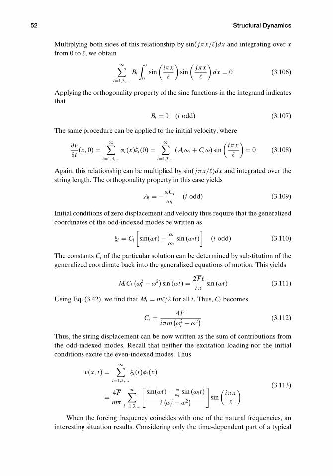
52 Structural Dynamics
Multiplying both sides of this relationship by sin( jπx/�)dx and integrating over xfrom 0 to �, we obtain
∞∑i=1,3,...
Bi
∫ �
0sin
(iπx�
)sin
(jπx�
)dx = 0 (3.106)
Applying the orthogonality property of the sine functions in the integrand indicatesthat
Bi = 0 (i odd) (3.107)
The same procedure can be applied to the initial velocity, where
∂v
∂t(x, 0) =
∞∑i=1,3,...
φi (x)ξi (0) =∞∑
i=1,3,...
(Aiωi + Ciω) sin(
iπx�
)= 0 (3.108)
Again, this relationship can be multiplied by sin( jπx/�)dx and integrated over thestring length. The orthogonality property in this case yields
Ai = −ωCi
ωi(i odd) (3.109)
Initial conditions of zero displacement and velocity thus require that the generalizedcoordinates of the odd-indexed modes be written as
ξi = Ci
[sin(ωt) − ω
ωisin (ωi t)
](i odd) (3.110)
The constants Ci of the particular solution can be determined by substitution of thegeneralized coordinate back into the generalized equations of motion. This yields
Mi Ci(ω2
i − ω2) sin (ωt) = 2F�
iπsin (ωt) (3.111)
Using Eq. (3.42), we find that Mi = m�/2 for all i . Thus, Ci becomes
Ci = 4F
iπm(ω2
i − ω2) (3.112)
Thus, the string displacement can be now written as the sum of contributions fromthe odd-indexed modes. Recall that neither the excitation loading nor the initialconditions excite the even-indexed modes. Thus
v(x, t) =∞∑
i=1,3,...
ξi (t)φi (x)
= 4Fmπ
∞∑i=1,3,...
[sin(ωt) − ω
ωisin (ωi t)
i(ω2
i − ω2)
]sin
(iπx�
) (3.113)
When the forcing frequency coincides with one of the natural frequencies, aninteresting situation results. Considering only the time-dependent part of a typical

3.1 Uniform String Dynamics 53
Figure 3.9. String with concentratedforce at mid-span
term in the series of Eq. (3.113), that is
sin(ωt) − ωωi
sin (ωi t)
i(ω2
i − ω2) (3.114)
we find that when ω → ωi , the term becomes indeterminate. To see what its value isin the limit, we let ωi = ω + εi , which gives
sin(ωt) − ωω+εi
sin [(ω + εi ) t]
i[(ω + εi )
2 − ω2] (3.115)
Invoking l’Hopital’s rule to take the limit as εi → 0, we obtain
sin(ωt) − ωt cos(ωt)2iω2
(3.116)
The second term tends to infinity as time increases with a linearly increasing ampli-tude. This phenomenon is called “resonance” and, because of its destructive nature,should be avoided. That is, when a structure is excited using harmonic excitation, theforcing frequency must not be too near any of the structure’s natural frequencies.
Example: Calculation of Forced Response with Nonzero-Initial Conditions. A sec-ond example is considered to illustrate the treatment of a concentrated force andinitial conditions that are not identically zero. In this case, a concentrated step-function force of magnitude F0 is applied to the center of the string, as illustrated inFig. 3.9. Recall that the unit-step function, 1(t), is defined by
1(t) = 0 (t < 0)
= 1 (t ≥ 0)(3.117)
The initial shape of the string is given as
v(x, 0) = h sin(
4πx�
)(3.118)
and the initial velocity as zero.
54 Structural Dynamics
The generalized force can be determined from the integral of a distributedloading as
�i =∫ �
0f (x, t)φi (x)dx
=∫ �
0F01(t)δ
(x − �
2
)φi (x)dx
= F01(t)φi
(�
2
)
= F01(t) sin(
iπ2
)(3.119)
because
sin(
iπ2
)= 0 (i even)
= (−1)i−1
2 (i odd)(3.120)
the generalized equations of motion become
Mi (ξi + ω2i ξi ) = 0 (i even)
Mi (ξi + ω2i ξi ) = F01(t)(−1)
i−12 (i odd)
(3.121)
The corresponding general solutions are
ξi = Ai sin (ωi t) + Bi cos (ωi t) (i even)
ξi = Ai sin (ωi t) + Bi cos (ωi t) + Ci (i odd)(3.122)
Consider the finite, initial displacement
v(x, 0) =∞∑
i=1
ξi (0)φi (x)
=∞∑
i=2,4,...
Bi sin(
iπx�
)+
∞∑i=1,3,...
(Bi + Ci ) sin(
iπx�
)
= h sin(
4πx�
)(3.123)
This last equality is multiplied by sin( jπx/�)dx and integrated over the length of thestring to yield
h∫ �
0sin
(4πx�
)sin
(jπx�
)dx =
∞∑i=2,4,...
Bi
∫ �
0sin
(iπx�
)sin
(jπx�
)dx
+∞∑
i=1,3,...
(Bi + Ci )∫ �
0sin
(iπx�
)sin
(jπx�
)dx
(3.124)

3.2 Uniform Beam Torsional Dynamics 55
These integrals can be evaluated easily by noting the orthogonality property of thesine functions. The result gives the following values for the constants Bi :
B4 = h
Bi = 0 (i even but �= 4) (3.125)
Bi = −Ci (i odd)
The initial velocity being zero requires that
∂v
∂t(x, 0) =
∞∑i=1
ξi (0)φi (x) =∞∑
i=1
ωi Ai sin(
iπx�
)= 0 (3.126)
Multiplication by sin( jπx/�)dx and integration results in determining that Ai = 0for all i . These results can be summarized by noting that ξi = 0 for all even values ofi except
ξ4 = h cos (ω4t) (3.127)
and for odd i
ξi = Ci [1 − cos (ωi t)] (i odd) (3.128)
The constants Ci can be determined by substitution of the odd generalizedcoordinates back into the equations of motion
Mi Ciω2i = F0(−1)
i−12 t ≥ 0 (3.129)
Given that Mi = m�/2, this yields
Ci = 2�F0(−1)i−1
2
T(iπ)2(3.130)
so that the complete string displacement becomes
v(x, t) =∞∑
i=1
ξi (t)φi (x)
= h cos (ω4t) sin(
4πx�
)+ 2�F0
Tπ2
∞∑i=1,3,...
(−1)i−1
2
i2 [1 − cos (ωi t)] sin(
iπx�
)
(3.131)
Thus, the first term is the response due to initial displacement, and the sum over theodd-indexed modes is the response due to the forcing function.
3.2 Uniform Beam Torsional Dynamics
Although vibrating strings are easy to visualize and exhibit many of the features ofvibrating aerospace structures, to analyze such structures, more realistic models areneeded. In this section, we apply the concepts related to the modal representation

56 Structural Dynamics
to the dynamics of beams in torsion. A beam is a structural member in which onedimension is much larger than the other two. It is thus understandable to idealize thetwisting and bending of high-aspect-ratio wings and helicopter rotor blades in termsof beam theory, especially in conceptual and preliminary design. Because manybehavioral characteristics of typical aeronautical structures are found in beams, thetorsion of beam-like lifting surfaces plays a vital role in both static and dynamicaeroelasticity.
3.2.1 Equations of Motion
For free vibration of a beam in torsion, we specialize the equation of motion derivedin Section 2.3.1 by setting r(x, t) = 0 to obtain
∂
∂x
[GJ (x)
∂θ
∂x
]= ρ Ip(x)
∂2θ
∂t2(3.132)
Other than the quantities that multiply the partial derivatives, this equation of motionis similar to that for the dynamic behavior of a string. The difference is that thestiffness coefficient GJ (x), unlike the tension in the string, may not be constant.Specialization to the spanwise uniform case is undertaken to obtain a closed-formsolution. Properties varying with x are not an obstacle for application of the varietyof approximate methods discussed in Section 3.5, but here we are concerned withobtaining closed-form solutions to aid in understanding the results. As shown whenwe explore the boundary conditions in detail, there are more interesting possibilitiesfor the boundary conditions for beams in torsion than there are for the string.
As before, we apply separation of variables, by substituting
θ(x, t) = X(x)Y(t) (3.133)
into the partial differential equation of motion and arranging the terms so thatdependencies on x and t are separated across the equality. This yields[
GJ (x)X ′(x)]′
ρ Ip(x)X(x)= Y(t)
Y(t)(3.134)
Thus, each side must equal a constant—say, −ω2—so that[GJ (x)X ′(x)
]′ρ Ip(x)X(x)
= Y(t)Y(t)
= −ω2 (3.135)
Two ordinary differential equations then follow; namely
[GJ (x)X ′(x)]′ + ρ Ip(x)ω2 X(x) = 0
Y(t) + ω2Y(t) = 0(3.136)
The first of Eqs. (3.136) has variable coefficients in x and—except for certain specialcases such as spanwise uniformity—does not possess a closed-form solution. Thesecond, however, is the same as the second of Eqs. (3.6), the solution of which is wellknown.

3.2 Uniform Beam Torsional Dynamics 57
Some specialization is necessary in order to proceed further. Therefore, weconsider only beams with spanwise uniform properties. Eqs. (3.136) then become
X ′′ + α2 X = 0
Y + ω2Y = 0(3.137)
where α2 = ρ Ipω2/GJ . For α �= 0, the solutions can be written as
X(x) = Asin(αx) + Bcos(αx)
Y(t) = C sin (ωt) + Dcos (ωt)(3.138)
To complete the solutions, constants A and B can be determined to within a mul-tiplicative constant from the boundary conditions at the ends of the beam; C andD can be found as a function of the initial beam deflection and rate of deflection.Because the partial differential equations of motion governing both transverse vibra-tion of uniform strings and torsional vibration of uniform beams are one-dimensionalwave equations, we rightfully can expect all of the previously discussed propertiesof standing and traveling waves to exist here as well.
Note that the special case of α = 0 is an important special case with a differentset of general solutions. It is addressed in more detail in Section 3.2.3.
3.2.2 Boundary Conditions
For a beam undergoing pure torsion, one boundary condition is required at each end.Mathematically, boundary conditions may affect θ as well as its partial derivatives,such as ∂θ/∂x and ∂2θ/∂t2, at the ends of the beam. In the context of the separationof variables, these conditions lead to corresponding conditions on X and/or X ′ atthe ends. These relationships are necessary and sufficient for determination of theconstants Aand B to within a multiplicative constant.
The nature of the boundary condition at an end stems from how that end isrestrained. When an end cross section is unrestrained, the tractions on it are identi-cally zero. Conversely, the most stringent condition is a perfect clamp, which allowsno rotation of an end cross section. Although this is a common idealization, it ispractically impossible to achieve in practice.
Cases that only partially restrain an end cross section involve elastic and/orinertial reactions. For example, an aircraft wing attached to a flexible support, suchas a fuselage, is not a perfect clamped condition; the root of the wing experiencessome rotation because of inherent flexibility at the point of attachment. A boundarycondition that is idealized in terms of a rotational spring may be used to createa more realistic model for the support flexibility. Appropriate values for supportflexibility can be estimated from static tests. Boundary conditions involving inertialreactions may stem from attached rigid bodies to model the effects of fuel tanks,engines, armaments, and so on.

58 Structural Dynamics
Figure 3.10. Clamped end of a beam
In this section, we consider two boundary conditions of the “primitive” type andtwo examples of derived boundary conditions that can be imposed at the ends of thebeam to determine the constants Aand B.
Clamped End. In this first primitive case (Fig. 3.10), the x = � end of the beam isassumed to be clamped or rigidly attached to an immovable support. As a conse-quence, there is no rotation due to elastic twist at this end of the beam, and theboundary condition is
θ(�, t) = 0 = X(�)Y(t) (3.139)
which is identically satisfied when
X(�) = 0 (3.140)
Free End. For the second primitive case, we consider the x = � end cross section ofthe beam to be free of stress (Fig. 3.11). Therefore, the twisting moment resultanton the end cross section must be zero
T(�, t) = GJ (�)∂ θ
∂x(�, t) = 0 (3.141)
Because GJ (�) > 0, this specializes to
∂θ
∂x(�, t) = X ′(�)Y(t) = 0 (3.142)
Thus, the specific condition to be satisfied is
X ′(�) = 0 (3.143)
Other Forms of End Restraint. In any cross section of a beam undergoing deforma-tion, there is a set of tractions on the plane of a typical cross section; a traction is aprojection of the stress (three-dimensional) onto a surface (two-dimensional). Fromtractions at a given cross section, we can define the resultant force and moment atthat station of the beam. When the end of a beam is connected to a rigid body, the
Figure 3.11. Free end of a beam

3.2 Uniform Beam Torsional Dynamics 59
=
Figure 3.12. Schematic of the x = � end of thebeam, showing the twisting moment T, and theequal and opposite torque acting on the rigid body
body exerts forces and moments on the beam that are balanced by the distributedtraction on the end cross section. That is, the force and moment resultants on theend cross section are reacted by equal and opposite forces and moments on the rigidbody. These facts, along with application of suitable laws of motion for the attachedbody, allow us to determine the boundary conditions.
In the case of torsion, for any cross section, the resultant moment about x oftractions caused by transverse shearing stress has the sense of a twisting moment, T,given by
T ≡ GJ∂θ
∂x(3.144)
With x directed to the right and the outward-directed normal along the positive xdirection at the end of the beam where x = �, a positive twisting moment is directedalong x in the right-handed sense. To avoid coupling with transverse motion, westipulate that the mass center C of the attached rigid body lies on the x axis (i.e., theelastic axis of the beam). The body has a mass moment of inertia IC about C so thatit contributes a concentrated rotational inertia effect on the beam. The free-bodydiagram for the problem is then as shown in Fig. 3.12. By Newton’s third law, thebeam’s twisting moment produces an equal and opposite torque on the rigid body.
Recall that Euler’s second law for a rigid body is stated precisely in Section 2.1.2.The only forces acting on the rigid body here3 are the contact forces from the beam.So, the x component of the left-hand side of Euler’s law is the sum of all momentsacting on the body; that is (∑
Mc
)x
≡ −T(�, t) (3.145)
where the sign in front of T is negative because of the free-body diagram and the signconvention, which has moments acting on the body as positive in the same directionas the rotation of the body—along x in the right-handed sense. The x component ofthe right-hand side is the inertial time derivative of the inertial angular momentumabout C, here simply the moment of inertia times the angular acceleration:( F dHc
dt
)x
≡ IC∂2θ
∂t2(�, t) (3.146)
where the left superscript on the left-hand side reflects the fact that the time deriva-tive is taken in the inertial frame F , defined in Section 2.1.2. Euler’s law for this rigid
3 Recall that we normally ignore gravity for free-vibration problems.

60 Structural Dynamics
=
Figure 3.13. Schematic of the x = 0 end of thebeam, showing the twisting moment T, and theequal and opposite torque acting on the rigid body
body is then expressed by equating these two very different quantities, yielding
−T(�, t) = IC∂2θ
∂t2(�, t) (3.147)
or
−GJ∂θ
∂x(�, t) = IC
∂2θ
∂t2(�, t) (3.148)
This equation then expresses the boundary condition of a beam undergoing uncou-pled torsional vibration with a rigid body attached at x = �.
When the body is attached to the x = 0 end, there is a subtle but importantdifference. With x directed to the right and the outward-directed normal along thenegative x direction at the x = 0 end of the beam, a positive twisting moment isdirected along −x in the right-handed sense. The free-body diagram for the problemis then as shown in Fig. 3.13. By Newton’s third law, the twisting moment producesan equal and opposite torque on the rigid body, which is in the direction of a positiverotation for the body. Therefore, Euler’s law (and the resulting boundary condition)is written as
T(0, t) = IC∂2θ
∂t2(0, t) (3.149)
or
GJ∂θ
∂x(0, t) = IC
∂2θ
∂t2(0, t) (3.150)
Thus, this equation expresses the boundary condition of a beam undergoing uncou-pled torsional vibration with a rigid body attached at x = 0.
The following example illustrates a convenient way to think about the contri-bution of a spring to the boundary of a beam undergoing only torsional rotation.Consider a beam with an attached rigid body at its x = � end, such that the rigidbody is, in turn, restrained by a light torsional spring attached to the ground. Therotational sign convention does not change; θ is always positive in the x direction(i.e., to the right in the sense of the right-hand rule). The rigid body, because it isattached to the end of the beam, rotates by θ(�, t). Thus, the rotational spring reactsagainst that rotation, and the moment applied by the spring to the body is oppositeto the direction of the rotation (Fig. 3.14). The boundary condition for the beamresults from applying Euler’s second law to the rigid body, so that
−kθ(�, t) − T(�, t) = IC∂2θ
∂t2(�, t) (3.151)

3.2 Uniform Beam Torsional Dynamics 61
θ
θ
=
Figure 3.14. Example with rigid body and spring
If the body-spring mechanism is instead on the x = 0 end of the beam, then themoment exerted by the spring is still in the same direction. However, what constitutesa positive twisting moment on the beam has the opposite sense, and the boundarycondition changes to
−kθ(0, t) + T(0, t) = IC∂2θ
∂t2(0, t) (3.152)
Clearly, if the body is absent, one may set IC = 0. Then, the problem reducesto the elastically restrained boundary condition, as shown in Fig. 3.15. The twistingmoment at the beam end must be equal and opposite to the spring reaction for anyfinite rotation due to twist at the x = � end, so that
−T(�, t) = −GJ∂θ
∂x(�, t) = kθ(�, t) (3.153)
At the x = 0 end, however
T(0, t) = GJ∂θ
∂x(0, t) = kθ(0, t) (3.154)
To be useful for separation of variables, we must determine the correspondingboundary condition on X. Thus, we write θ(x, t) as X(x)Y(t) as before, yielding
GJ X ′(�)Y(t) = −kX(�)Y(t) (3.155)
which requires that
GJ X ′(�) = −kX(�) (3.156)
Readers should verify that the same type of boundary condition at the other endwould yield
GJ X ′(0) = kX(0) (3.157)
where the sign change comes about by virtue of the switch in the direction notedpreviously for a positive twisting moment.
Figure 3.15. Elastically restrained end of abeam

62 Structural Dynamics
=
Figure 3.16. Inertially restrained end of a beam
Conversely, if the spring is absent, we may set k = 0, and the problem reducesto the inertially restrained case with only a rigid body attached to the x = � end(Fig. 3.16). The twisting moment at the beam end must be equal and opposite to theinertial reaction of the concentrated inertia for any finite angular acceleration of theend. Therefore
−GJ∂θ
∂x(�, t) = IC
∂2θ
∂t2(�, t) (3.158)
Expressing this condition in terms of X(x), Y(t), and their derivatives, we find that
−GJ X ′(�)Y(t) = IC X(�)Y(t) (3.159)
From separation of variables, it was determined from the second of Eqs. (3.137) thatfor free vibration (i.e., no external forces), we may regard Y(t) as describing simpleharmonic motion; that is
Y(t) = −ω2Y(t) = −α2GJ
ρ IpY(t) (3.160)
Substitution into the preceding condition then yields
GJ X ′(�)Y(t) = α2 GJ
ρ IpIC X(�)Y(t) (3.161)
which requires that
ρ Ip X ′(�) = α2 IC X(�) (3.162)
As before, readers should verify that the same type of boundary condition at theother end would yield
ρ Ip X ′(0) = −α2 IC X(0) (3.163)
It is appropriate to note that the use of Eq. (3.160) allows us to express Eq. (3.158)as
GJ∂θ
∂x(�, t) = ω2 ICθ(�, t) (3.164)
with the caveat that this condition holds true only for simple harmonic motion.
3.2.3 Example Solutions for Mode Shapes and Frequencies
In this section, we consider several examples of the calculation of natural frequen-cies and mode shapes of vibrating beams in torsion. We begin with the clamped-free

3.2 Uniform Beam Torsional Dynamics 63
θ
= =
Figure 3.17. Schematic of clamped-free beam undergoing torsion
case, often referred to as “cantilevered.” Next, we consider the free-free case, illus-trating the concept of the rigid-body mode. Finally, we consider a case that requiresnumerical solution of the transcendental characteristic equation: a beam clamped atits root and restrained with a rotational spring at the tip.
Example Solution for Clamped-Free Beam. To illustrate the application of theseboundary conditions, consider the case of a uniform beam that is clamped at x = 0and free at x = �, as shown in Fig. 3.17. The boundary conditions for this case are
X(0) = X ′(�) = 0 (3.165)
Recall that the general solution was previously determined as
θ(x, t) = X(x)Y(t) (3.166)
where X and Y are given in Eqs. (3.138). For α �= 0, the first of those equations hasthe solution
X(x) = Asin(αx) + Bcos(αx) (3.167)
It is apparent that the boundary conditions lead to the following
X(0) = 0 requires B = 0
X ′(�) = 0 requires Aα cos(α�) = 0(3.168)
If A= 0, a trivial solution is obtained, such that the deflection is identically zero.Because α �= 0, a nontrivial solution requires that
cos(α�) = 0 (3.169)
This is called the “characteristic equation,” the solutions of which consist of a denu-merably infinite set called the “eigenvalues” and are given by
αi� = (2i − 1)π2
(i = 1, 2, . . .) (3.170)
The Y(t) portion of the general solution is observed to have the form of simpleharmonic motion, as indicated in Eq. (3.160), so that the natural frequency is
ω = α
√GJ
ρ Ip(3.171)

64 Structural Dynamics
0.2 0.4 0.6 0.8 1
x0.2
0.4
0.6
0.8
11 x
0.2 0.4 0.6 0.8 1
x
1
0.5
0.5
12 x
0.2 0.4 0.6 0.8 1
x
1
0.5
0.5
13 x
Figure 3.18. First three mode shapes for clamped-freebeam vibrating in torsion
Because α can have only specific values, the frequencies also take on specific numer-ical values given by
ωi = αi
√GJ
ρ Ip= (2i − 1)π
2�
√GJ
ρ Ip(3.172)
These are the natural frequencies of the beam. Associated with each frequency is a“mode shape” as determined from the x-dependent portion of the general solution.The mode shapes (or eigenfunctions) can be written as
φi (x) = sin(αi x) = sin[
(2i − 1)πx2�
](3.173)
or any constant times φi (x). The first three of these mode shapes are plotted inFig. 3.18. The zero derivative at the free end is indicative of the vanishing twistingmoment at the free end.
Example Solution for Free-Free Beam. A second example, which exhibits bothelastic motion as described previously and motion as a rigid body, is the case of a

3.2 Uniform Beam Torsional Dynamics 65
θ= =
Figure 3.19. Schematic of free-free beam undergoing torsion
beam that is free at both ends, as shown in Fig. 3.19. The boundary conditions are
X ′(0) = X ′(�) = 0 (3.174)
From the general solution for X(x) in Eqs. (3.138), we find that for α �= 0
X ′(x) = Aα cos(αx) − Bα sin(αx) (3.175)
Thus, the condition at x = 0 requires that
Aα = 0 (3.176)
For A= 0, the condition at x = � requires that
sin(α�) = 0 (3.177)
because a null solution (θ ≡ 0) is obtained if B = 0. This characteristic equation issatisfied by
αi� = iπ (i = 1, 2, . . .) (3.178)
and the corresponding natural frequencies become
ωi = iπ�
√GJ
ρ Ip(3.179)
The associated mode shapes are determined from the corresponding X(x) as
φi (x) = cos(αi x) = cos(
iπx�
)(3.180)
These frequencies and mode shapes describe the normal mode of vibration for theelastic degrees of freedom of the free-free beam in torsion.
Now, if in the previous analysis the separation constant, α, is taken as zero, thenthe governing ordinary differential equations are changed to
X ′′
X= ρ Ip
GJ
YY
= 0 (3.181)
or
X ′′(x) = 0 and Y(t) = 0 (3.182)
The general solutions to these equations can be written as
X(x) = ax + b
Y(t) = ct + d(3.183)
The arbitrary constants, a and b, in the spatially dependent portion of the solutionagain can be determined from the boundary conditions. For the present case of the

66 Structural Dynamics
free-free beam, the conditions are
X ′(0) = 0 requires a = 0
X ′(�) = 0 requires a = 0(3.184)
Because both conditions are satisfied without imposing any restrictions on the con-stant b, this constant can be anything, which implies that the torsional deflection canbe nontrivial for α = 0. From X(x) with a = 0, it is apparent that the correspondingvalue of θ is independent of the coordinate x. This means that this motion for α = 0is a “rigid-body” rotation of the beam.
The time-dependent solution for this motion, Y(t), also is different from thatobtained for the elastic motion. Primarily, the motion is not oscillatory; thus, therigid-body natural frequency is zero. The arbitrary constants, c and d, can be ob-tained from the initial values of the rigid-body orientation and angular velocity. Tosummarize the complete solution for the free-free beam in torsion, a set of general-ized coordinates can be defined by
θ(x, t) =∞∑
i=0
φi (x)ξi (t) (3.185)
where
φ0 = 1
φi = cos(
iπx�
)(i = 1, 2, . . .)
(3.186)
The first three elastic mode shapes are plotted in Fig. 3.20. The zero derivative at bothends is indicative of the vanishing twisting moment there. The natural frequenciesassociated with these mode shapes are
ω0 = 0
ωi = iπ�
√GJ
ρ Ip(i = 1, 2, . . .)
(3.187)
Note that the rigid-body generalized coordinate, ξ0(t), represents the radian measureof the rigid-body rotation of the beam about the x axis.
A quick way to verify the existence of a rigid-body mode is to substitute ω = 0and X = a constant into the differential equation, and boundary conditions for X.A rigid-body mode exists if and only if all are satisfied. Caution: Do not try to arguethat there is a rigid-body mode because α = 0 satisfies the characteristic equation,Eq. (3.177). To obtain that equation, we presupposed that α �= 0!
Example Solution for Clamped-Spring-Restrained Beam. A final example forbeam torsion is given by the system shown in Fig. 3.21. The beam is clamped atthe root (x = 0) end, and the other end is restrained with a rotational spring havingspring constant k = ζ GJ/�, where ζ is a dimensionless parameter. The boundary

3.2 Uniform Beam Torsional Dynamics 67
0.2 0.4 0.6 0.8 1
x
1
0.5
0.5
11 x
0.2 0.4 0.6 0.8 1
x
1
0.5
0.5
12 x
0.2 0.4 0.6 0.8 1
x
1
0.5
0.5
13 x
Figure 3.20. First three elastic mode shapes for free-freebeam vibrating in torsion
conditions on X are thus
X(0) = 0
GJ X ′(�) = −kX(�) = −GJ�
ζ X(�) → �X ′(�) + ζ X(�) = 0(3.188)
When these boundary conditions are substituted into the general solution found inEqs. (3.138), we see that the first condition requires that B = 0; the second condition,along with the requirement for a nontrivial solution, leads to
ζ tan(α�) + α� = 0 (3.189)
Figure 3.21. Schematic of torsion problem withspring

68 Structural Dynamics
2 4 6 8 10
4
2
2
4
ζ, tan α
α
α
Figure 3.22. Plots of tan(α�) and −α�/ζ versus α� for ζ = 5
This transcendental equation has a denumerably infinite set of roots that cannot befound in closed form. However, as many of these roots as desired can be found usingnumerical procedures found in commercially available software packages such asMathematica,TM Maple,TM and MATLAB.TM
To facilitate this sort of root-finding in general, we may need to specify initialguesses for the values of α�. These can be found using graphical means by plotting,for example, tan(α�) and −α�/ζ versus α� for a specified value of ζ = 5, as shownin Fig. 3.22. The points where these curves intersect (indicated by dots in the figure)are the solutions, the locations of which are seen to be approximately at α� = 2.6,5.4, and 8.4. These values, when used as initial guesses in a root-finding application,provide quick convergence to α1� = 2.65366, α2� = 5.45435, and α3� = 8.39135. Asan alternative approach for this particular example, we may solve Eq. 3.189 for ζ
and plot it versus α� to find the roots without iteration.Thus, the roots of Eq. (3.189) are functions of ζ , and the first four such roots are
plotted versus ζ in Fig. 3.23. Denoting these roots by αi , with i = 1, 2, . . . , we obtainthe corresponding natural frequencies
ωi = αi
√GJ
ρ Ip(i = 1, 2, . . .) (3.190)
From the plots (and from Eq. 3.189), we note that as ζ tends toward zero, α1� tendstoward π/2, which means that the fundamental natural frequency is
ω1 = π
2�
√GJ
ρ Ip(ζ → 0) (3.191)
which is the natural frequency of a clamped-free beam in torsion (as shown herein).We also can show that as ζ tends to infinity, α1� tends toward π so that the

3.2 Uniform Beam Torsional Dynamics 69
20 40 60 80 100
2
4
6
8
10
12
i
Figure 3.23. Plot of the lowest values of αi versus ζ for a clamped-spring-restrained beam intorsion
fundamental natural frequency is
ω1 = π
�
√GJ
ρ Ip(ζ → ∞) (3.192)
which is the natural frequency of a clamped-clamped beam in torsion. Recalling thesimilarity of the governing equations and boundary conditions, the determination ofthe natural frequencies of a clamped-clamped beam in torsion follows directly fromthe previous solution for natural frequencies of a string fixed at both ends.
To obtain the corresponding mode shapes, we take the solutions for αi andsubstitute back into X, recalling that we can arbitrarily set A= 1 and that B = 0.The resulting mode shape is
φi = sin(αi x) (i = 1, 2, . . .) (3.193)
The first three modes for ζ = 1 are shown in Fig. 3.24. As expected, neither the twistangle nor its derivative are equal to zero at the tip. Close examination of Fig. 3.24illustrates that for higher and higher frequencies, the spring-restrained ends behavemore and more like free ends.
3.2.4 Calculation of Forced Response
The formulation of initial-value problems for beams in torsion is almost identicalto that for strings, presented in Section 3.1.7. We first should determine the virtualwork done by the applied loads, such as a distributed twisting moment per unitlength discussed in Section 2.3.1. From this, we may find the generalized forcesassociated with torsion. Once the generalized forces are known, we may solve thegeneralized equations of motion, which are of the form in Eq. (3.90). The resultinginitial-value problem then can be solved by invoking orthogonality to obtain values

70 Structural Dynamics
0.2 0.4 0.6 0.8 1
x0.2
0.4
0.6
0.8
11 1
0.2 0.4 0.6 0.8 1
x
1
0.5
0.5
12 1
0.2 0.4 0.6 0.8 1
x
1
0.5
0.5
13 1
Figure 3.24. First three mode shapes for clamped-spring-restrained beam in torsion, ζ = 1
of the arbitrary constants in the general and particular solutions, as illustrated in theexamples in Section 3.1.7.
3.3 Uniform Beam Bending Dynamics
The free vibration of a beam in bending is often referred to as “transverse vibration.”This type of motion differs from the transverse dynamics of strings and the torsionaldynamics of beams in that the governing equations of motion are of a differentmathematical form. Although these equations are different, their solutions are ob-tained in a similar manner and exhibit similar physical characteristics. Again, westart with the properties varying with x and specialize when we must. Observe thatwhereas most aerospace structures experience combined or simultaneous bendingand torsional dynamic behavior, we have here chosen certain configuration variablesto uncouple these types of motion.
3.3.1 Equation of Motion
From Section 2.3.2, Eq. (2.53) is repeated here for convenience
∂2
∂x2
(EI
∂2v
∂x2
)+ m
∂2v
∂t2= f (x, t) (3.194)
3.3 Uniform Beam Bending Dynamics 71
In the following sections, we treat the special case of free vibration for whichf (x, t) = 0.
3.3.2 General Solutions
A solution to the equation of motion for the transverse vibrations of beams can beobtained by a separation of the independent variables. This separation is denoted as
v(x, t) = X(x)Y(t) (3.195)
which, when substituted into the equation of motion, yields
(EI X ′′)′′
mX= − Y
Y(3.196)
Because the dependencies on x and t were separated across the equality, each sidemust equal a constant—say, ω2. The resulting ordinary differential equations thenbecome
(EI X ′′)′′ − mω2 X = 0
Y + ω2Y = 0(3.197)
For simplicity, we specialize the equations for the case of spanwise uniformityof all properties so that the first of Eqs. (3.197) simplifies to
X ′′′′ = α4 X (3.198)
where
α4 = mω2
EI(3.199)
is a constant.For α �= 0, the general solution to the second of Eqs. (3.197) can be written as
in the cases for the string and beam torsion; namely
Y(t) = Asin(ωt) + Bcos(ωt) (3.200)
For α �= 0, the general solution to the spatially dependent equation can beobtained by presuming a solution of the form
X(x) = exp(λx) (3.201)
Substitution of this assumed form into the fourth-order differential equation forX(x) yields
λ4 − α4 = 0 (3.202)
which can be factored to
(λ − iα)(λ + iα)(λ − α)(λ + α) = 0 (3.203)
indicating a general solution of the form
X(x) = C1 exp(iαx) + C2 exp(−iαx) + C3 exp(αx) + C4 exp(−αx) (3.204)

72 Structural Dynamics
Rewriting the exponential functions as trigonometric and hyperbolic sine and cosinefunctions yields an alternative form of the general solution as
X(x) = D1 sin(αx) + D2 cos(αx) + D3 sinh(αx) + D4 cosh(αx) (3.205)
Eventual determination of the constants Di (i = 1, 2, 3, and 4) and α requires spec-ification of appropriate boundary conditions. To facilitate this procedure, this lastsolution form can be rearranged to provide, in some cases, a slight advantage in thealgebra, so that
X(x) = E1[sin(αx) + sinh(αx)] + E2[sin(αx) − sinh(αx)]
+ E3[cos(αx) + cosh(αx)] + E4[cos(αx) − cosh(αx)](3.206)
To complete the solution, the constants Aand B can be determined from the initialdeflection and rate of deflection of the beam. The remaining four constants, Ci , Di ,or Ei (i = 1, 2, 3, and 4), can be evaluated from the boundary conditions, which mustbe imposed at each end of the beam. As was true for torsion, the important specialcase of α = 0 is connected with rigid-body modes for beam bending and is addressedin more detail in Section 3.3.4.
3.3.3 Boundary Conditions
For the beam-bending problem, it is necessary to impose two boundary conditionsat each end of the beam. Mathematically, boundary conditions may affect v and itspartial derivatives, such as ∂v/∂x, ∂2v/∂x2, ∂3v/∂x3, ∂2v/∂t2, and ∂3v/∂x∂t2. In thecontext of the separation of variables, these conditions lead to corresponding con-straints on some or all of the following at the ends: X, X ′, X ′′, and X ′′′. The resultingfour boundary conditions on X and its derivatives are necessary and sufficient fordetermination of the four constants Ci , Di , or Ei (i = 1, 2, 3, and 4) to within amultiplicative constant.
As with torsion, the nature of the boundary conditions at an end stems fromhow that end is restrained. When an end cross section is unrestrained, the tractionson it are identically zero. Again, the most stringent condition is a perfect clamp,which for bending allows neither translation nor rotation of an end cross section.Like the clamped-end condition in torsion, the clamped end in bending is a commonidealization, although nearly impossible to achieve in practice.
For the bending problem, a wide variety of cases that only partially restrainan end cross section is possible. The cases typically involve elastic and/or inertialreactions. A boundary condition that is idealized in terms of both translational androtational springs may be used to more realistically account for support flexibility.Appropriate values for both translational and rotational flexibility of the supportcan be estimated from static tests. Finally, we can use rigid bodies and springs incombination to model attached hardware such as fuel tanks, engines, armaments,and laboratory fixtures.

3.3 Uniform Beam Bending Dynamics 73
=
Figure 3.25. Schematic of pinned-end condition
In this section, we consider the four “primitive” boundary conditions; four de-rived boundary conditions involving individual elastic and inertial restraints; andtwo examples of derived boundary conditions that involve combinations of v and itspartial derivatives that can be imposed at the ends of the beam for determination ofthe four arbitrary constants of the general solution for X.
A boundary condition can be written as a linear relationship involving one ormore of the following: the beam deflection, its first three spatial partial derivatives,and its first two temporal partial derivatives. Although it is not a mathematicalrequirement, the particular combination of conditions to be specified at a beamend should represent a physically realizable constraint. The various spatial partialderivatives of the beam deflection can be associated with particular beam states atany arbitrary point along the beam. There are four such states of practical interest:
1. Deflection = v(x, t) = X(x)Y(t)2. Slope = β(x, t) = ∂v
∂x (x, t) = X ′(x)Y(t)
3. Bending Moment = M(x, t) = EI(x) ∂2v∂x2 (x, t) = EI(x)X ′′(x)Y(t)
4. Shear = V(x, t) = − ∂∂x
[EI(x) ∂2v(x,t)
∂x2
]= −[EI(x)X ′′(x)]′Y(t)
When relating these beam states, the positive convention for deflection and slopeis the same at both ends of the beam. In contrast, the sign conventions on shearand bending moment differ at opposite beam ends, as illustrated by the free-bodydifferential beam element used to obtain the equation of motion (see Fig. 2.6).
The most common conditions that can occur at the beam ends involve vanish-ing pairs of individual states. Typical of such conditions are the following classicalconfigurations (specialized for spanwise uniformity):
� Clamped or built-in end, which implies zero deflection and slope, is illustratedin Fig. 3.10 and has v(�, t) = ∂v
∂x (�, t) = 0 so that X(�) = X ′(�) = 0.� Free end, which corresponds to zero bending moment and shear, is illustrated
in Fig. 3.11 and has M(�, t) = V(�, t) = 0 so that X ′′(�) = X ′′′(�) = 0.� Simply supported, hinged, or pinned end, which indicates zero deflection and
bending moment, is denoted by the triangular symbol in Fig. 3.25 and hasv(�, t) = M(�, t) = 0 so that X(�) = X ′′(�) = 0.
� Sliding end, which corresponds to zero shear and slope, is illustrated in Fig. 3.26and has ∂v
∂x (�, t) = V(�, t) = 0 so that X ′(�) = X ′′′(�) = 0.
All of these conditions can occur in the same form at x = 0.

74 Structural Dynamics
Figure 3.26. Schematic of sliding-end condition
In addition to these zero-state conditions, we derive boundary conditions corre-sponding to linear-constraint reactions associated with elastic and inertial elements.The simplest of these are of the following four basic types:
� translational elastic constraint� rotational elastic constraint� translational inertia constraint� rotational inertia constraint
Two additional examples are presented that are more involved because they entailcombinations of these four types.
Translational Elastic Constraint. Consider a beam undergoing bending with a trans-lational spring with elastic constant k attached to the x = 0 end of a beam, as shownin Fig. 3.27. Assuming that this end of the beam is deflected by the amount v(0, t),then the spring tries to pull the end of the beam back to its original position byexerting a downward force at the end, the magnitude of which is equal to kv(0, t).Because the transverse-shear force at the left end (on the negative x face) is positivedown, the boundary condition becomes
V(0, t) = kv(0, t) (3.207)
Using the definition of the shear force, we obtain
− ∂
∂x
(EI
∂2v
∂x2
)(0, t) = kv(0, t) (3.208)
To be useful for separation of variables, we must make the substitution v(x, t) =X(x)Y(t), yielding
[EI(0)X(0)′′]′ = −kX(0) (3.209)
Figure 3.27. Example beam undergoing bending with a spring at the x = 0 end

3.3 Uniform Beam Bending Dynamics 75
= =
Figure 3.28. Schematic of beam with translational spring at both ends
which further simplifies for a spanwise uniform beam to
EI X ′′′(0) = −kX(0) (3.210)
If the spring were at x = � instead, the direction of the spring force at x = �
would be the same (i.e., downward), but the shear force is positive upward becausethis is the positive x face. Thus
V(�, t) = −kv(�, t) (3.211)
and
[EI(�)X(�)′′]′ = kX(�) (3.212)
which further simplifies for a spanwise uniform beam to
EI X ′′′(�) = kX(�) (3.213)
These conditions must be augmented by one additional condition at each endbecause two are required. For example, consider a beam with translational springsat both ends, as shown in Fig. 3.28. At each end, the other conditions for this casewould be that the bending moment is equal to zero.
Rotational Elastic Constraint. Consider now a beam with a rotational spring at theright end, as depicted in Fig. 3.29. For a rotation of the end cross-sectional plane of∂v/∂x at x = �, which is positive in the counterclockwise direction, the spring exertsa moment in the opposite direction (i.e., clockwise). Because the bending moment atthe right end of the beam is positive in the counterclockwise direction, the boundarycondition then becomes
M(�, t) = −k∂v
∂x(�, t) (3.214)
Figure 3.29. Example of beam undergoing bending with a rotational spring at right end

76 Structural Dynamics
= =
Figure 3.30. Schematic of beam with rotational springs at both ends
Using the definition of bending moment, we find
EI∂2v
∂x2(�, t) = −k
∂v
∂x(�, t) (3.215)
The boundary condition on X then becomes
EI X ′′(�) = −kX ′(�) (3.216)
As with the shear force, the sign convention on bending moment differs atthe opposite end. Here, at the left end, the spring still exerts a clockwise moment;however, the bending moment is also positive in the clockwise direction. Thus, wemay write
M(0, t) = k∂v
∂x(0, t)
EI∂2v
∂x2(0, t) = k
∂v
∂x(0, t)
(3.217)
for the condition on v(x, t) and its partial derivatives and
EI X ′′(0) = kX ′(0) (3.218)
for that on X(x) and its derivatives. As before, one more condition is required ateach end. Consider, for example, a beam with rotational springs at both ends, shownin Fig. 3.30. Here, it is necessary to set the shear forces at both ends equal to zero.
Translational and Rotational Inertia Constraints. The translational inertia con-straint stems from the inertial reaction force associated with the translational motionof either a rigid body or a particle attached to an end of a beam. Similarly, the ro-tational inertia constraint results from the inertial reaction moment associated withrotational motion of a rigid body attached to an end of a beam.
Consider the beam shown in Fig. 3.31, to which is attached a rigid body of massmc and mass moment of inertia about the mass center C equal to IC. The pointC is located on the x axis at x = 0, and the beam is assumed to be undergoingbending deformation. The set of all contact forces exerted on the body by thebeam can be replaced by a single force applied at the point C, and the moment ofthose contact forces about C. The resultant of all of those contact forces is simplythe shear force V(0, t); their moment about C is the bending moment M(0, t).

3.3 Uniform Beam Bending Dynamics 77
=
Figure 3.31. Schematic of rigid body (a) attached to end of a beam, and (b) detached showinginteractions
Therefore, Euler’s first and second laws take on the form
V(0, t) = mc∂2v
∂t2(0, t)
M(0, t) = IC∂2v
∂x∂t2(0, t)
(3.219)
which in terms of v and its partial derivatives become, respectively,
− ∂
∂x
[EI(0)
∂2v
∂x2(0, t)
]= mc
∂2v
∂t2(0, t)
EI(0)∂2v
∂x2(0, t) = IC
∂2v
∂x∂t2(0, t)
(3.220)
To determine the boundary conditions on X, we first substitute v(x, t) = X(x)Y(t)as before, yielding
−[EI(0)X ′′(0)]′Y(t) = mc X(0)Y(t)
EI(0)X ′′(0)Y(t) = IC X ′(0)Y(t)(3.221)
Recalling from the second of Eqs. (3.197) that Y + ω2Y = 0, these relationshipssimplify to
−[EI(0)X ′′(0)]′ = −mcω2 X(0)
EI(0)X ′′(0) = − ICω2 X ′(0)(3.222)
which, for a spanwise uniform beam, may be simplified to
mX ′′′(0) = mcα4 X(0)
mX ′′(0) = − ICα4 X ′(0)(3.223)
Eqs. (3.223) apply when a rigid body is attached to a free end. For a particle, we maysimply set IC = 0. Finally, at the opposite end of the beam, we need only change thesigns of the stress resultants, so that
−V(�, t) = mc∂2v
∂t2(0, t)
−M(�, t) = IC∂3v
∂x∂t2(0, t)
(3.224)

78 Structural Dynamics
=
Figure 3.32. Example with rigid body attached to the right end of beam undergoing bending
from which we may express boundary conditions on X for a spanwise uniform beam,given by
mX ′′′(�) = −mcα4 X(�)
mX ′′(�) = ICα4 X ′(�)(3.225)
It is appropriate to note that the use of the second of Eqs. (3.225) allows us toexpress Eqs. (3.197) as
V(�, t) = mcω2v(0, t)
M(�, t) = ICω2 ∂v
∂x(0, t)
(3.226)
subject to the restriction that these conditions hold true only for free vibration.
Other Boundary Configurations. We now turn our attention to two more examples,which are only slightly more involved. First, we consider a beam with an attachedrigid body of mass mc and moment inertia about C given by IC. The body has amass center that is offset from the point of attachment (at x = �) by a distance e, asshown in Fig. 3.32. (This is unlike the previous case in which the body mass centerC is located at x = � and thus has e = 0; see Fig. 3.31.) The body mass center Cis assumed to be on the x axis so that transverse vibrations do not excite torsionalvibrations and vice versa. The sum of all forces acting on the body is(∑
F)
y≡ −V(�, t) (3.227)
Euler’s first law says that this should be equated to the mass times the accelerationof C. The acceleration of C in the y direction can be written as
aCy = ∂2v
∂t2(�, t) + e
∂3v
∂t2∂x(�, t) (3.228)
where the body’s angular acceleration about the z axis (normal to the plane of thepaper) is
αz = ∂3v
∂t2∂x(�, t) (3.229)
Thus, Euler’s first law for the body is
−V(�, t) = mc
[∂2v
∂t2(�, t) + e
∂3v
∂t2∂x(�, t)
](3.230)

3.3 Uniform Beam Bending Dynamics 79
Figure 3.33. Example with mechanism attached to the left end of beam undergoing bending
The sum of the moments about C in the z direction(∑MC
)z≡ −M(�, t) + eV(�, t) (3.231)
Euler’s second law says that this should be equated to the moment of inertia aboutC times the angular acceleration about the z axis, so that
−M(�, t) + eV(�, t) = IC∂3v
∂t2∂x(�, t) (3.232)
Eqs. (3.230) and (3.232) can be combined to solve for V(�, t) and M(�, t), yielding
M(�, t) = −(IC + mce2)∂3v
∂t2∂x(�, t) − mce
∂2v
∂t2(�, t)
V(�, t) = −mc
[∂2v
∂t2(�, t) + e
∂3v
∂t2∂x(�, t)
] (3.233)
where the beam reactions are
M(�, t) ≡ EI(�)∂2v
∂x2(�, t)
V(�, t) ≡ − ∂
∂x
[EI(�)
∂2v
∂x2(�, t)
] (3.234)
The last example involves a mechanism attached to the left end of a beam witha pinned connection to ground, as shown in Fig. 3.33. The massless rigid rod is oflength h and the particle has mass mc; this combination should be considered a rigidbody with mass mc and moment of inertia about the pivot mch2. The massless rodis embedded in the left end of the beam and rotates with it. A positive rotationof the x = 0 cross-sectional plane about the normal to the page (i.e., the z axis) iscounterclockwise and has the value
β(0, t) = ∂v
∂x(0, t) (3.235)
This rotation results in the downward motion of the particle by the distance hβ(0, t)and leads to the upward force exerted by the spring, khβ(0, t). Thus, this body hasa free-body diagram, as shown in Fig. 3.34. A rotation of the rigid body is positivein the counterclockwise direction. Denoting the pivot as O, we find that the sum ofmoments on the mechanism is(∑
MO
)z≡ M(0, t) − kh2 ∂v
∂x(0, t) (3.236)
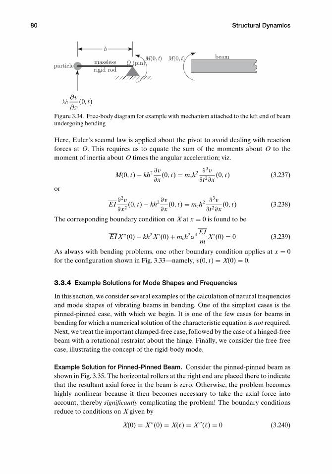
80 Structural Dynamics
Figure 3.34. Free-body diagram for example with mechanism attached to the left end of beamundergoing bending
Here, Euler’s second law is applied about the pivot to avoid dealing with reactionforces at O. This requires us to equate the sum of the moments about O to themoment of inertia about O times the angular acceleration; viz.
M(0, t) − kh2 ∂v
∂x(0, t) = mch2 ∂3v
∂t2∂x(0, t) (3.237)
or
EI∂2v
∂x2(0, t) − kh2 ∂v
∂x(0, t) = mch2 ∂3v
∂t2∂x(0, t) (3.238)
The corresponding boundary condition on X at x = 0 is found to be
EI X ′′(0) − kh2 X ′(0) + mch2α4 EIm
X ′(0) = 0 (3.239)
As always with bending problems, one other boundary condition applies at x = 0for the configuration shown in Fig. 3.33—namely, v(0, t) = X(0) = 0.
3.3.4 Example Solutions for Mode Shapes and Frequencies
In this section, we consider several examples of the calculation of natural frequenciesand mode shapes of vibrating beams in bending. One of the simplest cases is thepinned-pinned case, with which we begin. It is one of the few cases for beams inbending for which a numerical solution of the characteristic equation is not required.Next, we treat the important clamped-free case, followed by the case of a hinged-freebeam with a rotational restraint about the hinge. Finally, we consider the free-freecase, illustrating the concept of the rigid-body mode.
Example Solution for Pinned-Pinned Beam. Consider the pinned-pinned beam asshown in Fig. 3.35. The horizontal rollers at the right end are placed there to indicatethat the resultant axial force in the beam is zero. Otherwise, the problem becomeshighly nonlinear because it then becomes necessary to take the axial force intoaccount, thereby significantly complicating the problem! The boundary conditionsreduce to conditions on X given by
X(0) = X ′′(0) = X(�) = X ′′(�) = 0 (3.240)

3.3 Uniform Beam Bending Dynamics 81
Figure 3.35. Schematic of pinned-pinned beam
Substituting the first two boundary conditions into the general solution as found inEq. (3.205), we find that
D2 + D4 = 0
α2(−D2 + D4) = 0(3.241)
Recall that the constant α cannot be zero. To consider the α = 0 case we must takea solution in the form of a cubic polynomial, and the boundary conditions for thiscase do not yield a nontrivial solution of that form. Therefore, D2 = D4 = 0, and thesolution for X becomes
X(x) = D1 sin(αx) + D3 sinh(αx) (3.242)
Using the last two of the boundary conditions, we obtain a set of homogeneousalgebraic equations in D1 and D3[
sin(α�) sinh(α�)
−sin(α�) sinh(α�)
]{D1
D3
}={
0
0
}(3.243)
A nontrivial solution can exist only if the determinant of the coefficients is equal tozero; therefore
2 sin(α�) sinh(α�) = 0 (3.244)
Because α �= 0, we know that the only way this characteristic equation can be satisfiedis for
sin(α�) = 0 (3.245)
which has a denumerably infinite set of roots given by
αi = iπ�
(i = 1, 2, . . .) (3.246)
Although this is the same set of eigenvalues that we found for the string problem,the relationship to the natural frequencies is quite different; viz.
ω2i = EIα4
i
m(3.247)
so that
ωi = α2i
√EIm
=(
iπ�
)2√
EIm
= (iπ)2
√EIm�4
(3.248)

82 Structural Dynamics
Figure 3.36. Schematic of clamped-free beam
As observed in the cases of the string and beam torsion, there is associatedwith the ith natural frequency a unique deformation shape called the mode shape(or eigenfunction). Each mode shape can be obtained from the spatially dependentportion of the solution by evaluating the function, Xi (x), for any known value of αi .To find Xi , we substitute any value for αi back into either of the two scalar equationsrepresented by the matrix equation in Eq. (3.243). It is important to recognize thatthe constants D1 and D3 now should be written as D1i and D3i . Using the first ofthese equations along with the knowledge that sinh(αi�) �= 0, we find that D3i = 0,leaving
Xi = D1i sin(
iπx�
)(i = 1, 2, . . .) (3.249)
where D1i can be any nonzero constant. For example, choosing D1i = 1, we find themode shape to be
φi = sin(
iπx�
)(i = 1, 2, . . .) (3.250)
which is the same mode shape as obtained previously for the vibrating string.
Example Solution for Clamped-Free Beam. Consider the clamped-free beam asshown in Fig. 3.36, the boundary conditions of which reduce to conditions on Xgiven by
X(0) = X ′(0) = X ′′(�) = X ′′′(�) = 0 (3.251)
As in the previous example, we can show that this problem does not exhibit anontrivial solution for the case of α = 0. Thus, we use the form of the general solutionin Eq. (3.206) for which α �= 0. Along with the first two boundary conditions, thisyields
X(0) = 0 → E3 = 0
X ′(0) = 0 → E1 = 0(3.252)
The remaining boundary conditions yield two homogeneous algebraic equations thatmay be reduced to the form[
sinh(α�) + sin(α�) cosh(α�) + cos(α�)
cosh(α�) + cos(α�) sinh(α�) − sin(α�)
]{E2
E4
}={
0
0
}(3.253)
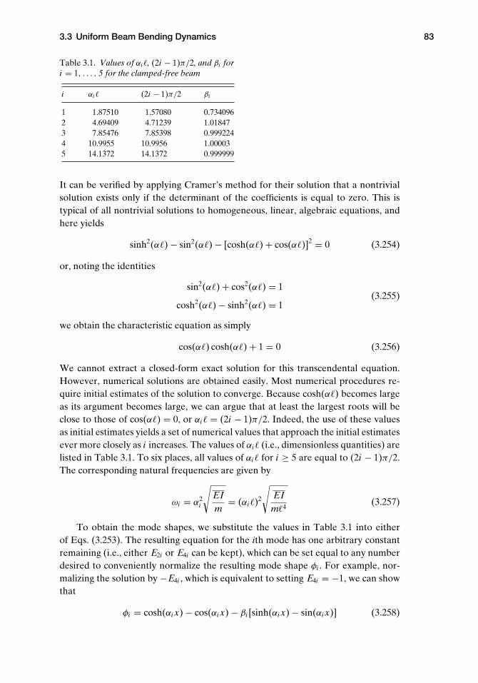
3.3 Uniform Beam Bending Dynamics 83
Table 3.1. Values of αi�, (2i − 1)π/2, and βi fori = 1, . . . , 5 for the clamped-free beam
i αi � (2i − 1)π/2 βi
1 1.87510 1.57080 0.7340962 4.69409 4.71239 1.018473 7.85476 7.85398 0.9992244 10.9955 10.9956 1.000035 14.1372 14.1372 0.999999
It can be verified by applying Cramer’s method for their solution that a nontrivialsolution exists only if the determinant of the coefficients is equal to zero. This istypical of all nontrivial solutions to homogeneous, linear, algebraic equations, andhere yields
sinh2(α�) − sin2(α�) − [cosh(α�) + cos(α�)]2 = 0 (3.254)
or, noting the identities
sin2(α�) + cos2(α�) = 1
cosh2(α�) − sinh2(α�) = 1(3.255)
we obtain the characteristic equation as simply
cos(α�) cosh(α�) + 1 = 0 (3.256)
We cannot extract a closed-form exact solution for this transcendental equation.However, numerical solutions are obtained easily. Most numerical procedures re-quire initial estimates of the solution to converge. Because cosh(α�) becomes largeas its argument becomes large, we can argue that at least the largest roots will beclose to those of cos(α�) = 0, or αi� = (2i − 1)π/2. Indeed, the use of these valuesas initial estimates yields a set of numerical values that approach the initial estimatesever more closely as i increases. The values of αi� (i.e., dimensionless quantities) arelisted in Table 3.1. To six places, all values of αi� for i ≥ 5 are equal to (2i − 1)π/2.The corresponding natural frequencies are given by
ωi = α2i
√EIm
= (αi�)2
√EIm�4
(3.257)
To obtain the mode shapes, we substitute the values in Table 3.1 into eitherof Eqs. (3.253). The resulting equation for the ith mode has one arbitrary constantremaining (i.e., either E2i or E4i can be kept), which can be set equal to any numberdesired to conveniently normalize the resulting mode shape φi . For example, nor-malizing the solution by −E4i , which is equivalent to setting E4i = −1, we can showthat
φi = cosh(αi x) − cos(αi x) − βi [sinh(αi x) − sin(αi x)] (3.258)

84 Structural Dynamics
0.2 0.4 0.6 0.8 1
x
0.5
1
1.5
21
0.2 0.4 0.6 0.8 1
x
21.5
10.5
0.51
1.52
0.2 0.4 0.6 0.8 1
x
10.5
0.51
1.52
3
Figure 3.37. First three free-vibration mode shapes of aclamped-free beam in bending
where
βi = − E2i
E4i= cosh(αi�) + cos(αi�)
sinh(αi�) + sin(αi�)(3.259)
The values of βi also are tabulated in Table 3.1. For this particular normalization
∫ �
0φ2
i dx = �
φi (�) = 2(−1)i+1
(3.260)
the first of which is left to the reader to show (see Prob. 10d). The first three modeshapes are depicted in Fig. 3.37. Note that as with previous results, the higher themode number, the more nodes (i.e., crossings of the zero-displacement line).
Example Solution for Spring-Restrained, Hinged-Free Beam. This sample prob-lem for which modes of vibration are determined is for a uniform beam that ishinged at the right-hand end and restrained there by a rotational spring with elastic

3.3 Uniform Beam Bending Dynamics 85
==
Figure 3.38. Schematic of spring-restrained,hinged-free beam
constant k = κ EI/�. The left-hand end is free, as illustrated in Fig. 3.38. The bound-ary conditions for this case require that
X ′′(0) = 0
X ′′′(0) = 0
X(�) = 0
EI X ′′(�) = −kX ′(�) or �X ′′(�) = −κ X ′(�)
(3.261)
The spatially dependent portion of the general solution is used in the form ofEq. (3.206). The two conditions of zero bending moment and shear at x = 0 re-quire that
X ′′(0) = 0 → E4 = 0
X ′′′(0) = 0 → E2 = 0(3.262)
The third boundary condition, that of zero displacement at x = �, can now be indi-cated by
X(�) = E1 [sin(α�) + sinh(α�)] + E3 [cos(α�) + cosh(α�)] = 0 (3.263)
The fourth boundary condition, a rotational elastic constraint at x = �, can be writtenas
�2 X ′′(�) + κ�X ′(�) = 0 (3.264)
so that
(α�)2 {E1 [−sin(α�) + sinh(α�)] + E3 [−cos(α�) + cosh(α�)]}
+ κα�{
E1 [cos(α�) + cosh(α�)] + E3 [−sin(α�) + sinh(α�)]} = 0
(3.265)
This relationship can be rearranged as
E1
{cos(α�) + cosh(α�) + α�
κ[−sin(α�) + sinh(α�)]
}
+ E3
{−sin(α�) + sinh(α�) + α�
κ[− cos(α�) + cosh(α�)]
}= 0
(3.266)
The simultaneous solution of Eqs. (3.263) and (3.266) for nonzero values of E1 andE3 requires that the determinant of the 2×2 array formed by their coefficients must

86 Structural Dynamics
be zero. Setting the determinant formed from Eqs. (3.263) and (3.266) to zero, wefind
[sin(α�) + sinh(α�)]{
sin(α�) − sinh(α�) + α�
κ[cos(α�) − cosh(α�)]
}
+ [cos(α�) + cosh(α�)]{
cos(α�) + cosh(α�) + α�
κ[− sin(α�) + sinh(α�)]
}= 0
(3.267)
After executing the indicated multiplications and applying the identities ofEqs. (3.255), the relationship becomes(
α�
κ
)[sin(α�) cosh(α�) − cos(α�) sinh(α�)] = 1 + cos(α�) cosh(α�) (3.268)
This is the characteristic equation. As in the previous example, it is a transcendentalequation that cannot be solved analytically. Note that for specified finite and nonzerovalues of κ , we may calculate numerically a denumerably infinite set of the eigen-values αi� (for i = 1, 2, . . .) by a suitable iterative procedure. For such an iterativesolution, we need initial estimates for the α�s. Note, however, that this equation is aspecial case in which we may solve for κ as a function of α� without iteration.
In the limit as κ tends to infinity, we find eigenvalues in agreement with theclamped-free case, as expected. In the limit as κ tends to zero, we can show thata rigid-body mode exists. The next example illustrates a procedure by which wemay prove the existence of one or more rigid-body modes. It is important to note,however, that it is incorrect to try to infer the existence of a rigid-body mode becauseα� = 0 satisfies Eq. (3.268) in the limit as κ tends to zero; our general solution for Xis valid only when α �= 0.
For specified values of m, EI, �, and the stiffness parameter κ , the eigenvaluescan be used to determine the natural frequencies as
ωi = α2i
√EIm
= (αi�)2
√EIm�4
(i = 1, 2, . . .) (3.269)
and the ith mode shape can be defined as
φi (x) = Xi (x)E1i
= sin(αi x) + sinh(αi x) + βi [cos(αi x) + cosh(αi x)]
(3.270)
The modal parameter βi = E3i/E1i can be obtained from the zero-displacementboundary condition at x = �, Eq. (3.263). When evaluated for the ith mode, βi
becomes
βi = E3i
E1i= − sin(αi�) + sinh(αi�)
cos(αi�) + cosh(αi�)(3.271)
numerical values of which can be found once αi� is known for specific values of κ .A sample set of numerical results for this example is shown in Figs. 3.39 through
3.41. The first three mode shapes are shown for κ = 1 in Fig. 3.39. Fig. 3.40 shows thevariation of αi� versus κ for i = 1, 2, and 3, illustrating the fact that the frequencies of

3.3 Uniform Beam Bending Dynamics 87
0.2 0.4 0.6 0.8 1
x
2
1.5
1
0.5
1
0.2 0.4 0.6 0.8 1
x
21.5
10.5
0.51
2
0.2 0.4 0.6 0.8 1
x
21.5
10.5
0.51
3
Figure 3.39. Mode shapes for first three modes of aspring-restrained, hinged-free beam in bending; κ = 1,
ω1 = (1.24792)2√
EI/(m�4), ω2 =(4.03114)2
√EI/(m�4), and ω3 = (7.13413)2
√EI/(m�4)
the higher modes are much less sensitive to the spring constant than that of the firstmode. Indeed, the first mode frequency (proportional to the square of the smallestplotted quantity in Fig. 3.40) tends to zero as κ tends toward zero in the limit.This can be interpreted as the lowest-frequency mode transitioning to a rigid-bodymode, which exists only when the spring constant is identically zero. In the limit as κ
becomes infinite, in contrast, the eigenvalues tend toward those of the clamped-freebeam, as expected. Indeed, as Fig. 3.41 shows, when κ = 50 the mode shape starts
2 4 6 8 10
1
2
3
4
5
6
7
i
Figure 3.40. Variation of lowest eigenvalues αi� ver-sus dimensionless spring constant κ

88 Structural Dynamics
0.2 0.4 0.6 0.8 1
2.5
2
1.5
1
0.5
1 x
Figure 3.41. Mode shape for fundamentalmode of the spring-restrained, hinged-free beam in bending; κ = 50, ω1 =(1.83929)2
√EI/(m�4)
to look more like that of a clamped-free beam (with the fixity being on the right endin this example).
Example Solution for Free-Free Beam. The case of a uniform beam that is uncon-strained at both ends, Fig. 3.42, may be considered as a crude first approximation toa freely flying vehicle. Their elastic and rigid dynamic properties are quite similar. Inboth instances, these properties can be described in terms of a modal representation.
The boundary conditions for this case require that
X ′′(0) = X ′′′(0) = X ′′(�) = X ′′′(�) = 0 (3.272)
The spatially dependent portion of the general solution to be used here again involvesthe sums and differences of the trigonometric and hyperbolic functions. Two of theEi s can be eliminated by applying the boundary conditions at x = 0 so that
X ′′(0) = 0 → E4 = 0
X ′′′(0) = 0 → E2 = 0(3.273)
The conditions at x = � of zero bending moment and zero shear X ′′(�) = 0, andX ′′′(�) = 0, respectively, yield the following relationships:
E1 [− sin(α�) + sinh(α�)] + E3 [− cos(α�) + cosh(α�)] = 0
E1 [− cos(α�) + cosh(α�)] + E3 [sin(α�) + sinh(α�)] = 0(3.274)
Here again, the nontrivial solution to these equations requires that the determinantof the E1 and E3 coefficients be zero. This relationship becomes
sinh2(α�) − sin2(α�) − [cosh(α�) − cos(α�)]2 = 0 (3.275)
which simplifies to
cos(α�) cosh(α�) = 1 (3.276)
= =
Figure 3.42. Schematic of free-free beam

3.3 Uniform Beam Bending Dynamics 89
Table 3.2. Values of αi�, (2i + 1)π/2, and βi fori = 1, . . . , 5 for the free-free beam
i αi � (2i + 1)π/2 βi
1 4.73004 4.71239 0.9825022 7.85320 7.85398 1.000783 10.9956 10.9956 0.9999664 14.1372 14.1372 1.000005 17.2788 17.2788 1.00000
For large α�, the roots tend to values that make cos(α�) = 0. Unlike the clamped-freecase, however, there is no root near π/2, and the first nonzero root occurs near 3π/2.Indeed, the ith root is near (2i + 1)π/2. Thus, the roots of this characteristic equationreadily can be computed numerically to yield the eigenvalues αi� in Table 3.2. Fromthese numerical values, the natural frequencies can be found as
ωi = α2i
√EIm
(3.277)
The mode shape associated with each eigenvalue can be defined as
φi (x) = Xi (x)E3i
= cos(αi x) + cosh(αi x) − βi [sin(αi x) + sinh(αi x)]
(3.278)
The numerical value of the modal parameter βi = −E1i/E3i , also tabulated in Ta-ble 3.2, can be obtained from either of the boundary conditions given in Eqs. (3.274).Using the first of those equations as an example, we obtain
βi = − E1i
E3i= cosh(αi�) − cos(αi�)
sinh(αi�) − sin(αi�)(3.279)
It can be shown that the first of Eqs. (3.274) would yield the same result by usingthe characteristic equation as an identity. The first three of these mode shapes areshown in Fig. 3.43.
In addition to these modal properties that can be used to describe the elasticbehavior of the beam, there are also modal properties that describe the rigid be-havior of the beam. These modes are associated with zero values of the separationconstant α. Recall that a similar result was obtained for torsional deflections of afree-free beam. When α is zero, the governing ordinary differential equations forbeam bending, Eqs. (3.197), become
X ′′′′ = 0 Y = 0 (3.280)
The general solutions to these equations can be written as
X = b x3
6+ c x2
2+ d x + e
Y = f t + g
(3.281)

90 Structural Dynamics
0.2 0.4 0.6 0.8 1
x
1
0.5
0.5
1
1.5
21
0.2 0.4 0.6 0.8 1
x
2
1
1
22
0.2 0.4 0.6 0.8 1
x
10.5
0.51
1.52
3
Figure 3.43. First three free-vibration elastic modeshapes of a free-free beam in bending
where the arbitrary constants, b through e, in the spatially dependent portion of thesolution can be established from the boundary conditions. These conditions of zerobending moment and shear at the ends of the beam yield the following:
X ′′(0) = 0 → c = 0
X ′′′(0) = 0 → b = 0
X ′′(�) = 0 → b� + c = 0
X ′′′(�) = 0 → b = 0
(3.282)
It is apparent that all four boundary conditions can be satisfied with b = c = 0.Because no restrictions are placed on the constants d and e, they can be arbitrary.Thus, a general description of the solution in this case is
X = d x + e (3.283)
An important characteristic of this solution is that no relationship has been estab-lished between d and e. Therefore, they can be presumed to represent two inde-pendent motions of the beam. As written previously, e represents a rigid verticaltranslation of the beam because it is independent of x. The d x term, being linear

3.3 Uniform Beam Bending Dynamics 91
in x, represents a rigid rotation of the beam about the left end. It can be shownthat when the rotational motion is taken to be about the mass centroid, it and thetranslation are orthogonal with respect to one another and with respect to the elasticmodes. This suggests that the modal representation for these rigid-body degrees offreedom can be described by
vrigid =0∑
i=−1
φi (x)ξi (t) (3.284)
where
φ−1 = 1 and ξ−1(t) = translation
φ0 = x − �
2and ξ0(t) = rotation angle
(3.285)
The time-dependent portion of the solution for these rigid-body motions is seen tobe aperiodic. This means that natural frequencies for both rigid-body modes arezero. The two arbitrary constants contained in Y(t) can be evaluated from the initialrigid-body displacement and velocity associated with the translation and rotation.Thus, the complete solution for the free-free beam-bending problem can now bewritten in terms of all of its modes as
v =∞∑
i=−1
φi (x)ξi (t) (3.286)
This example provides a convenient vehicle for further discussion of symmetry.It was already noted in the case of a vibrating string that systems exhibiting geo-metric symmetry have two distinct types of mode shapes—namely, those that aresymmetric about the midpoint and those that are antisymmetric about the midpoint.As can be seen in the results, this is indeed true for the modes of the free-free beam.In particular, the rigid-body translation mode and the first and third elastic modesare clearly symmetric about the midpoint of the beam, whereas the rigid-body rota-tion mode and the second elastic mode are antisymmetric about the midpoint (seeFig. 3.43).
This observation suggests that the symmetric mode shapes could be obtained bycalculating the mode shapes of a beam that is half the length of the original beamand that has the sliding condition at one end and is free at the other. Similarly,the antisymmetric modes could be obtained by calculating the mode shapes of abeam with half the length of the original beam and that has one end pinned and theother free. It also should be evident that a symmetric aircraft with high-aspect-ratiowings, modeled as beams and attached to a rigid-body fuselage, could be representedsimilarly in terms of the symmetric and antisymmetric modes of the combined bodyand wing system. That is, we may model the whole system by considering only onewing attached to a rigid body with half the mass and half the rotational inertia withappropriate boundary conditions.

92 Structural Dynamics
3.3.5 Calculation of Forced Response
The formulation of initial-value problems for beams in bending is almost identicalto that for beams in torsion and for strings; see Sections 3.1.7 and 3.2.4, respectively.We should first determine the virtual work done by the applied loads, such as adistributed transverse force per unit length. From this, we may find the generalizedforces associated with bending. Once they are known, one may solve the generalizedequations of motion, which are in the form of Eq. (3.90). The resulting initial-value problem then can be solved by invoking orthogonality to obtain values ofthe arbitrary constants in the general and particular solutions, as illustrated in theexamples in Section 3.1.7.
3.4 Free Vibration of Beams in Coupled Bending and Torsion
In this section, the analytical treatment of coupled bending–torsion vibration ofcomposite beams is briefly considered. The treatment is restricted to uniform beamsand to the presentation of governing equations, sample boundary conditions, andsuggestions for solution.
3.4.1 Equations of Motion
First, we specialize Eqs. (2.65) for spanwise uniformity and free vibration, yielding
ρ Ip∂2θ
∂t2+ md
∂2v
∂t2− GJ
∂2θ
∂x2+ K
∂3v
∂x3= 0
md∂2θ
∂t2+ m
∂2v
∂t2+ EI
∂4v
∂x4− K
∂3θ
∂x3= 0
(3.287)
Because these are linear equations with constant coefficients, for free vibration wemay assume simple harmonic motion. In the spirit of separation of variables, thesolutions for v and θ are written as
v(x, t) = v(x) exp(iωt)
θ(x, t) = θ(x) exp(iωt)(3.288)
with the mode shapes being of the form
v = v exp(αx)
θ = θ exp(αx)(3.289)
which allows us to write the system of equations in matrix form as
[EIα4 − mω2 −Kα3 − mdω2
Kα3 − mdω2 −GJα2 − ρ Ipω2
]{v
θ
}={
00
}(3.290)

3.4 Free Vibration of Beams in Coupled Bending and Torsion 93
For there to be a nontrivial solution, the determinant of the coefficient matrix mustvanish, yielding
(EI GJ − K2)α6 + ρ Ip EIω2α4 − mGJω2α2 − (mρ Ip − m2d2)ω4 = 0 (3.291)
This cubic equation in α2 may be solved for arbitrary ω2. When d and K are nonzero,finding the exact, closed-form solution “by hand” is problematic. However, with theaid of symbolic computational tools such as MathematicaTM , we may easily extractthe six roots denoted here by αi for i = 1, 2, . . . , 6, as functions of ω2. Note thatαi+3 = −αi for i = 1, 2, and 3.
Therefore, when K, d �= 0, the solution for the mode shape may be written as
v = C1 exp(α1x) + C2 exp(α2x) + C3 exp(α3x)
+ C4 exp(−α1x) + C5 exp(−α2x) + C6 exp(−α3x)
θ = D1 exp(α1x) + D2 exp(α2x) + D3 exp(α3x)
+ D4 exp(−α1x) + D5 exp(−α2x) + D6 exp(−α3x)
(3.292)
where
Di = Ci
(Kα3
i − mdω2
GJα2i + ρ Ipω2
)i = 1, 2, . . . , 6 (3.293)
Now, with six boundary conditions (i.e., three at each end), we may find six homo-geneous algebraic equations for Ci . The condition for a nontrivial solution leads tothe characteristic equation for ω2. There is a denumerably infinite set of roots for ω2,so that for any value determined for ω2, we may find any five of the Ci coefficientsin terms of the sixth and thus determine the mode shapes. In general, each modeshape involves both v and θ . For small couplings (i.e., such that K2 � GJ EI andmd2 � ρ Ip), one “branch” of these roots is near the uncoupled bending frequenciesand the other is near the uncoupled torsional frequencies.
3.4.2 Boundary Conditions
The boundary conditions for coupled bending and torsion range from very simple tosomewhat complex, depending on the type of restraint(s) imposed on the ends. Forexample, for a clamped end, we have v = ∂v/∂x = θ = 0, the same as for uncoupledbending and torsion. Similarly, a free end has zero bending moment, shear force,and twisting moment, respectively written as M = V = T = 0. Note the definitionsof M and T in Eqs. (2.58) and that V = −∂ M/∂x. Equations governing other re-straints may be determined by appropriate kinematical or physical relationships.For example, a pinned connection may imply specification of an axis about whichthe moment vector (i.e., combination of bending and twisting moments) vanishesand perpendicular to which components of the rotation vector (i.e., combination ofbending and twisting rotations) vanish. Relationships for both elastic and inertialrestraints may be developed using Euler’s laws, as in the uncoupled cases herein.

94 Structural Dynamics
The complexity of this class of problem provides excellent motivation for theintroduction of approximate methods, which is undertaken in the next section.
3.5 Approximate Solution Techniques
There are several popular methods that make use of a set of modes or other functionsto approximate the dynamic behavior of systems. In this section, without goinginto detail about the theories associated with this subject, we illustrate within theframework already established how we can use a truncated set of modes or anotherset of functions to obtain an approximate solution. Details of the theories behindmodal approximation methods are found in texts that treat structural dynamics atthe graduate level. The two main approaches are (1) Galerkin’s method, appliedto ordinary or partial differential equations; and (2) the Ritz method, applied toLagrange’s equations or the principle of virtual work. These two methods yieldidentical results in certain situations. Thus, if time is limited, it would be necessary todiscuss only one of the two methods to give students an introduction to the methodand an appreciation of results that can be obtained this way. The Ritz method ispreferred in the present context because of the ease with which it can be presentedwithin the framework of Lagrange’s equations. Nevertheless, both of these methodsare presented at a level suitable for undergraduate students.
3.5.1 The Ritz Method
Building on the previous treatment, we start with Lagrange’s equations, given by
ddt
(∂L
∂ξi
)− ∂L
∂ξi= �i i = 1, 2, . . . , n (3.294)
where in the Lagrangean, L = K − P, the total kinetic energy is K, the total potentialenergy is P, n is the number of generalized coordinates retained, the generalizedcoordinates are ξi , and �i is the generalized force. Although it can be helpful, asdiscussed herein, it is not necessary to make use of potential energy, which canaccount only for conservative forces. The generalized force, however, can be used toinclude the effects of any loads. So as not to count the same physical effects more thanonce, the generalized force should include only those forces that are not accountedfor in the potential energy. The generalized forces stem from virtual work, whichcan be written as
δW =n∑
i=1
�iδξi (3.295)
where δξi is an arbitrary increment in the ith generalized coordinate.Consider a beam in bending as an example. The total kinetic energy must include
that of the beam as well as any attached particles or rigid bodies. The contribution

3.5 Approximate Solution Techniques 95
of the beam is
Kbeam = 12
∫ �
0m(
∂v
∂t
)2
dx (3.296)
where m is the mass per unit length of the beam. The total potential energy P =U + V comprises the internal strain energy of the beam, denoted by U, plus anyadditional potential energy, V, attributed to gravity, springs attached to the beam,or applied static loads. All other loads, such as aerodynamic loads, damping, andfollower forces, must be accounted for in �i .
The strain energy for a beam in bending is given by
U = 12
∫ �
0EI
(∂2v
∂x2
)2
dx (3.297)
The expression for V varies depending on the problem being addressed, as does thevirtual work of all forces other than those accounted for in V. The virtual work ofan applied distributed force per unit length f (x, t) can be written as
δW =∫ �
0f (x, t)δv(x, t)dx (3.298)
where δv is an increment of v in which time is held fixed and f (x, t) is positive in thedirection of positive v.
To apply the Ritz method, we need to express P, K, and δW in terms of a seriesof functions with one or more terms. For a beam in bending, this means that
v(x, t) =n∑
i=1
ξi (t)φi (x) (3.299)
There are several characteristics that these “basis functions” φi must possess, asfollows:
1. Each function must satisfy at least all boundary conditions on displacement androtation (often called the “geometric” boundary conditions). It is not necessarythat they satisfy the force and moment boundary conditions, but satisfaction ofthem may improve accuracy. However, it is not easy, in general, to find functionsthat satisfy all boundary conditions.
2. Each function must be continuous and p times differentiable, where p is theorder of the highest spatial derivative in the Lagrangean. The pth derivative ofat least one function must be nonzero. Here, from Eq. (3.297), p = 2.
3. If more than one function is used, they must be chosen from a set of functionsthat is complete. This means that any function on the interval 0 ≤ x ≤ � with thesame boundary conditions as the problem under consideration can be expressedto any degree of accuracy as a linear combination of the functions in the set.

96 Structural Dynamics
Examples of complete sets of functions on the interval 0 ≤ x ≤ � include
1, x, x2, . . .
sin(πx
�
), sin
(2πx�
), sin
(3πx�
), . . .
a set of mode shapes for any problem
Completeness also implies that there can be no missing terms between the lowestand highest terms used in any series.
4. The set of functions must be linearly independent. This means that
n∑i=0
aiφi (x) = 0 ⇒ ai = 0 for all i (3.300)
A set of functions that satisfies all of these criteria is said to be “admissible.”By use of the series approximation, we reduced a problem with an infinite
number of degrees of freedom to one with n degrees of freedom. Instead of beinggoverned by a partial differential equation, the behavior of this system is now definedby n second-order, ordinary differential equations in time. This reduction froma continuous system modeled by a partial differential equation with an infinitenumber of degrees of freedom to a system described by a finite number of ordinarydifferential equations in time is sometimes called spatial discretization. The numbern is usually increased until convergence is obtained. (Note that if inertial forces arenot considered so that the kinetic energy is identically zero, then a system describedby an ordinary differential equation in a single spatial variable is reduced by the Ritzmethod to a system described by n algebraic equations.)
Now, let us illustrate how the approximating functions are actually used. Let φi ,i = 1, 2, . . . , ∞, be a complete set of p-times differentiable, linearly independentfunctions that satisfy the displacement and rotation boundary conditions. Thus, Ucan be written as
U = 12
n∑i=1
n∑j=1
ξiξ j
∫ �
0EIφ′′
i φ′′j dx (3.301)
The contributions of any springs that restrain the structure, as well as conservativeloads, must be added to obtain the full potential energy P.
The kinetic energy of the beam is
Kbeam = 12
n∑i=1
n∑j=1
ξi ξ j
∫ �
0mφiφ j dx (3.302)
Contributions of any additional particles and rigid bodies must be added to obtainthe complete kinetic energy K.

3.5 Approximate Solution Techniques 97
The virtual work must account for distributed and concentrated forces resultingfrom all other sources, such as damping and aerodynamics. This can be written as
δW =n∑
i=1
δξi
[∫ �
0f (x, t)φi dx + Fc(x0, t)φi (x0)
](3.303)
where x0 is a value of x at which a concentrated force is located. Here, the firstterm accounts for a distributed force f (x, t) on the interior of the beam, and thesecond term accounts for a concentrated force on the interior (see Eq. 3.96). Inaeroelasticity, the loads f (x, t) and Fc(x0, t) may depend on the displacement in acomplicated manner.
The integrands in these quantities all involve the basis functions and their deriva-tives over the length of the beam. Note that these integrals involve only known quan-tities and often can be evaluated analytically. Sometimes they are too complicated toundertake analytically, however, and they must be evaluated numerically. Numeri-cal evaluation is often facilitated by nondimensionalization. Symbolic computationtools such as MathematicaTM and MapleTM may be helpful in both situations.
With all such things considered, the equations of motion can be written in a formthat is quite common; viz.
[M]{ξ}+ [C]
{ξ}+ [K] {ξ} = {F} (3.304)
where {ξ} is a column matrix of the generalized coordinates, {F} is a column matrix ofthe generalized force terms that do not depend on ξi , (˙) is the time derivative of ( ),[M] is the mass matrix, [C] is the gyroscopic/damping matrix, and [K] is the stiffnessmatrix. The most important contribution to [M] is from the kinetic energy, and thiscontribution is symmetric. The most important contribution to [K] is from the strainenergy of the structure and potential energy of any springs that restrain the motionof the structure. There can be contributions to all terms in the equations of motionfrom kinetic energy and virtual work. For example, there are contributions fromkinetic energy to [C] and [K] when there is a rotating coordinate system. Dampingmakes contributions to [C] through the virtual work. Finally, because aerodynamicloads, in general, depend on the displacement and its time derivatives, aeroelasticanalyses may contain terms in [M], [C], and [K] that stem from aerodynamic loads.
An interesting special case of this method occurs when the system is conser-vatively loaded. The resulting method is usually referred to as the Rayleigh–Ritzmethod, and many theorems can be proved about the convergence of approxima-tions to the natural frequency. Indeed, one of the most powerful of such theoremsstates that the approximate natural frequencies are always upper bounds; anotherstates that adding more terms to a given series always lowers the approximate naturalfrequencies (i.e., making them closer to the exact values).
A further specialized case is the simplest approximation, in which only one termis used. Then, an approximate expression for the lowest natural frequency can bewritten as a ratio called the “Rayleigh quotient.” This simplest special case is of morethan merely academic interest: It is not at all uncommon that a rough estimate ofthe lowest natural frequency is needed early in the design of flexible structures.

98 Structural Dynamics
Example: The Ritz Method Using Clamped-Free Modes. In the first example, weconsider a uniform, clamped-free beam that we modify by adding a tip mass ofmass μm�. The exact solution can be obtained easily for this modified problemusing the methodology described previously. However, it is desired here to illustratethe Ritz method, and we already calculated the modes for a clamped-free beam(i.e., without a tip mass) in Section 3.3.4. These mode shapes are solutions of aneigenvalue problem; therefore, provided we do not omit any modes between thelowest and highest mode number that we use, this set is automatically complete.The set is also orthogonal and therefore linearly independent. Of course, thesemodes automatically satisfy the boundary conditions on displacement and rotationfor our modified problem (because they are the same as for the clamped-free beam),and they are infinitely differentiable. Hence, they are admissible functions for themodified problem. Moreover, they satisfy the condition of zero moment at the freeend, which is a boundary condition for our modified problem. However, becauseof the presence of the tip mass in the modified problem, the shear force—whichreaders will recall is proportional to the third derivative of the displacement—doesnot vanish as it does for clamped-free mode shapes.
The strain energy becomes
U = 12
n∑i=1
n∑j=1
ξiξ j
∫ �
0EIφ′′
i φ′′j dx (3.305)
Substituting the mode shapes of Eq. (3.258) into Eq. (3.305) and taking advantageof orthogonality, we can simplify it to
U = �EI2
n∑i=1
ξ 2i α4
i (3.306)
where αi is the set of constants in Table 3.1. Similarly, accounting for the tip mass,the kinetic energy of which is
Ktip mass = 12μm�
[∂v
∂t(�, t)
]2
= 12μm�
n∑i=1
n∑j=1
ξi ξ jφi (�)φ j (�)
(3.307)
we obtain the total kinetic energy as
K = 12
n∑i=1
n∑j=1
ξi ξ j
[∫ �
0mφiφ j dx + μm�φi (�)φ j (�)
](3.308)
With the use of the mode shapes in Eq. (3.258), we find that φi (�) = 2(−1)i+1;therefore, the kinetic energy simplifies to
K = m�
2
n∑i=1
n∑j=1
ξi ξ j[δi j + 4μ(−1)i+ j ] (3.309)

3.5 Approximate Solution Techniques 99
Table 3.3. Approximate values of ω1
√m�4
EIfor
clamped-free beam with tip mass of μm� using nclamped-free modes of Section 3.3.4, Eq. (3.258)
n μ = 1 μ = 10 μ = 100
1 1.57241 0.549109 0.1755812 1.55964 0.542566 0.1733983 1.55803 0.541748 0.1731264 1.55761 0.541536 0.1730555 1.55746 0.541458 0.173029Exact 1.55730 0.541375 0.173001
where the Kronecker symbol δi j = 1 for i = j and δi j = 0 for i �= j . For free vibration,there are no additional forces. Thus, Lagrange’s equations now can be written inmatrix form as
[M]{ξ}+ [K] {ξ} = 0 (3.310)
where [`K`] is a diagonal matrix with the diagonal elements given by
Kii = EI�α4i i = 1, 2, . . . , n (3.311)
and [M] is a symmetric matrix with elements given by
Mi j = m�[δi j + 4μ(−1)i+ j ] i, j = 1, 2, . . . , n (3.312)
Assuming ξ = ξ exp(iωt), we can write Eq. (3.310) as an eigenvalue problem ofthe form [
[K] − ω2[M]] {
ξ} = 0 (3.313)
Results for the first modal frequency are shown in Table 3.3 and compared thereinwith the exact solution. As we can see, the approximate solution agrees with the exactsolution to within engineering accuracy with only two terms. For contrast, resultsfor the second modal frequency are shown in Table 3.4; these results are not nearlyas accurate. Results for the higher modes (not shown) are even less accurate. Thisis one of the problems with modal-approximation methods; fortunately, however,
Table 3.4. Approximate values of ω2
√m�4
EIfor
clamped-free beam with tip mass of μm� using nclamped-free modes of Section 3.3.4, Eq. (3.258)
n μ = 1 μ = 10 μ = 100
2 16.5580 15.8657 15.78673 16.3437 15.6191 15.53674 16.2902 15.5576 15.47445 16.2708 15.5353 15.4518Exact 16.2501 15.5115 15.4277

100 Structural Dynamics
Table 3.5. Approximate values of ω1
√m�4
EIfor
clamped-free beam with tip mass of μm� usingn polynomial functions
n μ = 1 μ = 10 μ = 100
1 1.55812 0.541379 0.1730012 1.55733 0.541375 0.1730013 1.55730 0.541375 0.1730014 1.55730 0.541375 0.1730015 1.55730 0.541375 0.173001Exact 1.55730 0.541375 0.173001
aeroelasticians and structural dynamicists frequently are interested in only the lower-frequency modes. Note that the one-term approximation (i.e., the Rayleigh quotient)is within 1.1% for all values of μ displayed.
Example: The Ritz Method Using a Simple Power Series. As an alternative to usingthe mode shapes of a closely related problem, let us repeat the previous solutionusing a simple power series to construct a series of functions φi . Because the momentvanishes at the free end where x = �, we can make the second derivative of all termsproportional to � − x. To obtain a complete series, we can multiply this term bya complete power series 1, x, x2, and so on. Thus, we then may write the secondderivative of the ith function as
φ′′i = 1
�2
(1 − x
�
) (x�
)i−1(3.314)
With the boundary conditions on displacement and rotation being φi (0) = φ′i (0) = 0,
we then can integrate to find an expression for the ith function as
φi =( x
�
)i+1 [2 + i − i( x
�
)]i (1 + i) (2 + i)
(3.315)
Because the chosen admissible functions have nonzero third derivatives at the tip,they offer the possibility of satisfying the nonzero shear condition in combinationwith one another. Such admissible functions are sometimes called “quasi-comparisonfunctions.”
In this case, the stiffness matrix becomes
Ki j = 2EI�3 (i + j − 1) (i + j) (1 + i + j)
i, j = 1, 2, . . . , n (3.316)
and the mass matrix
Mi j = 2m�[3(i2 + j2) + 7i j + 23(i + j) + 40
]i j (i + 1) (i + 2) ( j + 1) ( j + 2) (i + j + 3) (i + j + 4) (i + j + 5)
+ 4 μm�
i j (i + 1) (i + 2) ( j + 1) ( j + 2)i, j = 1, 2, . . . , n
(3.317)
Results from this calculation are given in Tables 3.5 and 3.6 for the first twomodes. It is clear that these results are much better than those obtained with the

3.5 Approximate Solution Techniques 101
Table 3.6. Approximate values of ω2
√m�4
EIfor
clamped-free beam with tip mass of μm� usingn polynomial functions
n μ = 1 μ = 10 μ = 100
2 16.2853 15.5443 15.46053 16.2841 15.5371 15.45244 16.2505 15.5119 15.42805 16.2501 15.5116 15.4277Exact 16.2501 15.5115 15.4277
clamped-free beam modes. It is not unusual for polynomial functions to providebetter results than those obtained with beam mode shapes. However, here it is worthnoting that the beam mode shapes are at a disadvantage for this problem. Unlikethe problem being solved (and the polynomials chosen), the beam mode shapesare constrained to have zero shear force at the free end and thus are not quasi-comparison functions for the problem with a tip mass. This one-term polynomialapproximation (i.e., the Rayleigh quotient) is within 0.05%, which is exceptionallygood given its simplicity.
It is sometimes suggested that the mode shapes of a closely related problemare—at least, in some sense—superior to other approximate sets of functions. Forexample, in the first example, we saw that the orthogonality of the modes used re-sulted in a diagonal stiffness matrix, which provides a slight advantage in the ease ofcomputing the eigenvalues. However, for the low-order problems of the sort we arediscussing, that advantage is hardly noticeable. Indeed, symbolic computation toolssuch as MathematicaTM and MapleTM are capable of calculating the eigenvalues forproblems of the size of this example in but a few seconds. Moreover, in some cases,the simplicity of carrying out the integrals that result in approximate formulations isa more important factor in deciding which set of functions to use in a standard im-plementation of the Ritz method. Indeed, polynomial functions are generally mucheasier to deal with analytically than free-vibration modes such as those illustrated inSection 3.5.1, which frequently involve transcendental functions.
Alternatives to the standard Ritz method include the methods of Galerkin, fi-nite elements, component mode synthesis, flexibility influence coefficients, methodsof weighted residuals, collocation methods, and integral equation methods. We in-troduce Galerkin’s method and the finite element method in the next two sections.Detailed descriptions of other approaches are found in more advanced texts onstructural dynamics and aeroelasticity.
3.5.2 Galerkin’s Method
Rather than making use of energy and Lagrange’s equation as in the Ritz method,Galerkin’s method starts with the partial differential equation of motion. Let usdenote this equation by
L[v(x, t)] = 0 (3.318)

102 Structural Dynamics
whereL is an operator on the unknown function v(x, t) with maximum spatial partialderivatives of the order q. For the structural dynamics problems addressed so far,the operator L is linear and q = 2p, where p is the maximum order of spatial partialderivative in the Lagrangean. It is important to note, however, that it is not true, ingeneral, that q = 2p; indeed, we do not need to consider the Lagrangean at all withthis method.
To apply Galerkin’s method, we need to express v(x, t) and, hence, the operatorL in terms of a series of functions with one or more terms. For a beam in bending,for example, this means that, as before
v(x, t) =n∑
j=1
ξ j (t)φ j (x) (3.319)
Relative to the basis functions used in the Ritz method, the characteristics that thesefunctions φi must possess for use in Galerkin’s method are more stringent, as follows:
1. Each function must satisfy all boundary conditions. Note that it is not easy, ingeneral, to find functions that satisfy all boundary conditions.
2. Each function must be at least q times differentiable. The qth derivative of atleast one function must be nonzero.
3. If more than one function is used, they must be chosen from a set of functionsthat is complete.
4. The set of functions must be linearly independent.
Functions that satisfy all of these criteria are said to be “comparison functions.”The original partial differential equation then is multiplied by φi and integrated overthe domain of the independent variable (e.g., 0 ≤ x ≤ �). Thus, a set of n ordinarydifferential equations is obtained from the original partial differential equation.(Note that if the original equation is an ordinary differential equation in x, thenGalerkin’s method yields n algebraic equations.)
Consider a beam in bending as an example. The equation of motion can bewritten as in Eq. (3.194), with a slight change, as
∂2
∂x2
(EI
∂2v
∂x2
)+ m
∂2v
∂t2− f (x, t) = 0 (3.320)
where EI is the flexural rigidity, m is the mass per unit length, and the boundaryconditions and loading term f (x, t) must reflect any attached particles or rigid bodies.In aeroelasticity, the loads f (x, t) may depend on the displacement in a complicatedmanner.
With all of the components as described herein considered, the discretized equa-tions of motion can be written in the same form as in the Ritz method; that is
[M]{ξ}+ [C]
{ξ}+ [K] {ξ} = {F} (3.321)
where {ξ} is a column matrix of the generalized coordinates, {F} is a column matrixof the generalized force terms that do not depend on ξi , (˙) is the time derivativeof ( ), [M] is the mass matrix, [C] is the gyroscopic/damping matrix, and [K] is the

3.5 Approximate Solution Techniques 103
stiffness matrix. As before, inertial forces contribute to [M], there are contributionsfrom the inertial forces to [C] and [K] when there is a rotating coordinate system,and damping also contributes to [C]. Finally, because aeroelastic loads, in general,depend on the displacement and its time derivatives, aerodynamics can contributeterms to [M], [C], and [K].
Example: Galerkin’s Method for a Beam in Bending. Now, we illustrate how theapproximating functions are actually used. Let φi , i = 1, 2, . . . , ∞ be a completeset of q-times differentiable, linearly independent functions that satisfy all of theboundary conditions. Substituting Eq. (3.319) into Eq. (3.320), multiplying by φi (x),and integrating over x from 0 to �, we obtain
∫ �
0φi
⎡⎣ n∑
j=1
ξ j (EIφ′′j )′′ +
n∑j=1
ξ j mφ j − f (x, t)
⎤⎦ dx = 0 i = 1, 2, . . . , n (3.322)
After reversing the order of integration and summation and integrating the firstterm by parts, and taking into account that the functions φi satisfy all the boundaryconditions, this equation becomes
n∑j=1
(ξ j
∫ �
0EIφ′′
i φ′′j dx + ξ j
∫ �
0mφiφ j dx
)−∫ �
0f φi dx = 0 i = 1, 2, . . . , n
(3.323)
When we compare the first two terms with the previous derivation by the Ritzmethod, we see the close relationship between these approaches. Indeed, if thestarting partial differential equation is derivable from energy—which implies thatq = 2p—and the same approximating functions φi are used in both cases, the result-ing discretized equations are the same.
Considering the clamped-free case, for example, we can develop a set of com-parison functions by starting with
φ′′i = 1
�2
(1 − x
�
)2 (x�
)i−1(3.324)
With the boundary conditions on displacement and rotation being φi (0) = φ′i (0) = 0,
we then can integrate to find an expression for the ith function as
φi =
(x�
)1+i{
6 + i2(
1 − x�
)2+ i
[5 − 6x
�+(x
�
)2]}
i(1 + i)(2 + i)(3 + i)(3.325)
Elements of the stiffness matrix are found as
Ki j =∫ �
0EIφ′′
i φ′′j dx
= 24EI�3 (i + j − 1) (i + j) (1 + i + j) (2 + i + j) (3 + i + j)
(3.326)

104 Structural Dynamics
Table 3.7. Approximate values of ωi
√m�4
EIfor
i = 1, 2, and 3, for a clamped-free beam usingn polynomial functions
n Mode 1 Mode 2 Mode 3
1 3.53009 – –2 3.51604 22.7125 –3 3.51602 22.0354 66.25624 3.51602 22.0354 61.76755 3.51602 22.0345 61.7395exact 3.51602 22.0345 61.6972
Similarly, the elements of the mass matrix are found as
Mi j =∫ �
0mφiφ j dx
= m�p1
p2
(3.327)
where
p1 = 30,240 + 28,512(i + j) + 9,672(i2 + j2) + 1,392(i3 + j3) + 72(i4 + j4)
+ 20,040i j + 4,520(i2 j + i j2) + 320(i3 j + i j3) + 520i2 j2
p2 = i(1 + i)(2 + i)(3 + i) j(1 + j)(2 + j)(3 + j)(3 + i + j)
(4 + i + j)(5 + i + j)(6 + i + j)(7 + i + j)(3.328)
The fact that the governing equation is derivable from energy is reflected in thesymmetry of [M] and [K]. Results for free vibration (i.e., with f = 0) are given inTable 3.7. As with the Ritz method, we see monotonic convergence from above andaccuracy comparable to that achieved via the Ritz method. However, unlike the Ritzmethod, we do not always obtain results for free-vibration problems that convergefrom above.
Example: Galerkin’s Method for a Beam in Bending Using an Alternative Formof the Equation of Motion. Consider again a clamped-free beam. To obtain analternative equation of motion, we integrate the equation of motion twice and usethe boundary conditions of zero shear and bending moment to obtain an integro-partial differential equation
EI∂2v
∂x2+∫ �
x(x − ζ )
[f (ζ, t) − m
∂2v(ζ, t)∂t2
]dζ = 0 (3.329)
where ζ is a dummy variable. Although this equation of motion is somewhat morecomplicated, it is only a second-order equation. Thus, it has only two boundaryconditions, which are zero displacement and slope at x = 0. Thus, a much simpler

3.5 Approximate Solution Techniques 105
Table 3.8. Approximate values of ωi
√m�4
EIfor
i = 1, 2, and 3 for a clamped-free beam using nterms of a power series with a reduced-orderequation of motion
n Mode 1 Mode 2 Mode 3
1 7.48331 – –2 3.84000 57.2822 –3 3.44050 24.1786 188.6774 3.52131 20.3280 69.38195 3.51698 22.0793 53.25586 3.51607 22.1525 61.0295exact 3.51602 22.0345 61.6972
set of comparison functions can be used, such as a simple power series; that is
φi =(x
�
)i+1i = 1, 2, . . . , n (3.330)
We should not expect greater accuracy from this simple set of functions, but theanalytical effort is considerably less. Indeed, the elements of the stiffness matrix are
Ki j =∫ �
0EIφiφ
′′j dx
= EI j( j + 1)�(i + j + 1)
(3.331)
and the elements of the mass matrix are
Mi j =∫ �
0φi
∫ �
x(ζ − x)mφ j (ζ )dζ dx
= m�3
(2 + i)(3 + i)(5 + i + j)
(3.332)
Note that these matrices are not symmetric. Moreover, the results presented inTable 3.8 are not as accurate as those obtained in Table 3.7, and the convergence isnot monotonic from above.
The partial differential equations derived previously for free vibration of strings,beams in torsion, and beams in bending can be derived from energy-based ap-proaches, such as Hamilton’s principle. (The use of Hamilton’s principle is beyondthe scope of this text, but detailed treatments are found in numerous graduate-leveltexts on structural dynamics.) In those cases, the Ritz and Galerkin’s methods givethe same results when used with the same approximating functions. As shown here,however, Galerkin’s method provides a viable alternative to the Ritz method incases where the equations of motion are not of the form presented previously in thischapter.

106 Structural Dynamics
Figure 3.44. Schematic of a nonuniform beam with distributed twisting moment per unitlength
3.5.3 The Finite Element Method
The finite element method is, by far, the most popular way of solving realisticstructural dynamics and aeroelasticity problems in industry. The name derives fromthe breaking of a structure into a large number of small elements, modeling themapproximately, and connecting them together appropriately. Because of this way ofdiscretizing the geometry, it is possible to accurately capture modeling details thatother methods cannot.
In one sense, the finite element method can be regarded as a special case of Ritzand Galerkin methods, one in which the generalized coordinates are themselves dis-placements and/or rotations at points along the structure. It typically makes use ofpolynomial shape functions over each of the finite elements into which the originalstructure is broken. Equations based on the finite element method have the samestructure as Eq. (3.304); however, they are typically of large order, with n beingon the order of 102 to 107. What keeps the computational effort from being overlyburdensome is that the matrices have a narrow-banded structure, which allows spe-cialized software to be used in solving the equations of motion that takes advantageof this structure, reducing both memory and floating-point operations and resultingin significant computational advantages.
Here, we present only a simple outline of the method as applied to beams intorsion and in bending, leaving more advanced topics such as plates and shells totextbooks devoted to the finite element method, such as those by Reddy (1993) andZienkiewicz and Taylor (2005).
Application to Beams in Torsion. Here, we use the finite element method to analyzethe behavior of a nonuniform beam in torsion. Similar to the application of the Ritzmethod, we make use of Lagrange’s equation. Regardless of how finite elements arederived, however, for a sufficiently fine mesh, the results should approach the exactstructural behavior. This development encompasses both forced response and freevibration.
Consider a clamped-free beam subjected to a distributed torque r(x, t) as de-picted in Fig. 3.44. Note that the x coordinate is along the beam. The strain energy
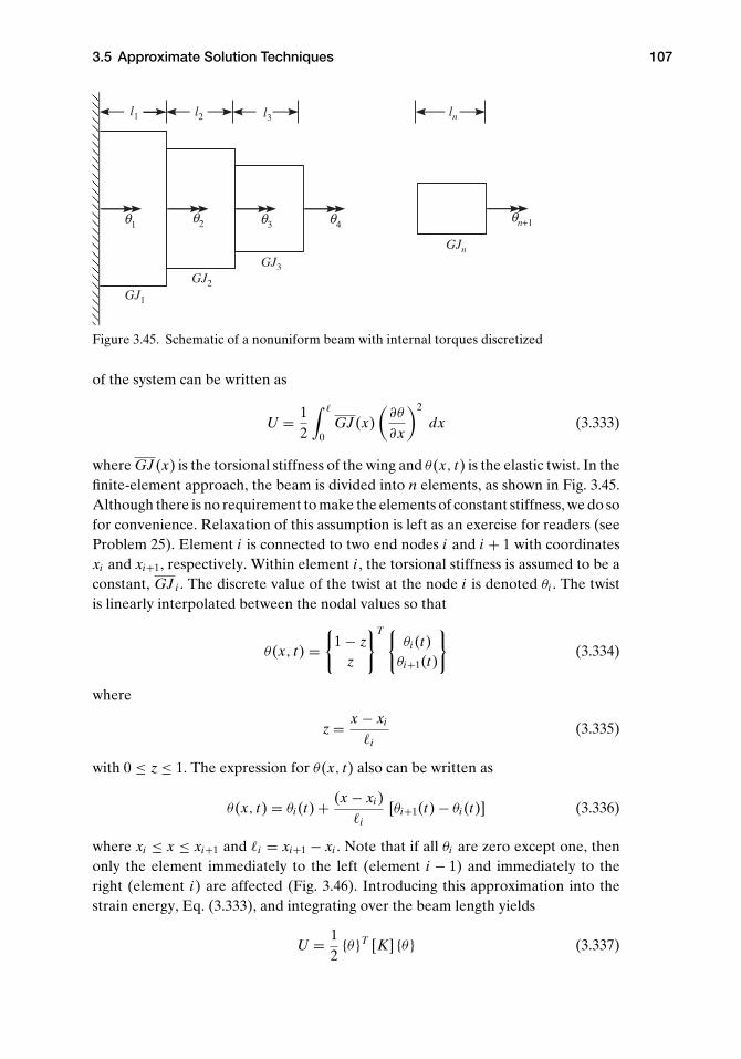
3.5 Approximate Solution Techniques 107
GJ1
GJ2
GJ3
GJn
θ1 θ2 θ4 θn+1
l1 l2 l3 ln
θ3
Figure 3.45. Schematic of a nonuniform beam with internal torques discretized
of the system can be written as
U = 12
∫ �
0GJ (x)
(∂θ
∂x
)2
dx (3.333)
where GJ (x) is the torsional stiffness of the wing and θ(x, t) is the elastic twist. In thefinite-element approach, the beam is divided into n elements, as shown in Fig. 3.45.Although there is no requirement to make the elements of constant stiffness, we do sofor convenience. Relaxation of this assumption is left as an exercise for readers (seeProblem 25). Element i is connected to two end nodes i and i + 1 with coordinatesxi and xi+1, respectively. Within element i , the torsional stiffness is assumed to be aconstant, GJ i . The discrete value of the twist at the node i is denoted θi . The twistis linearly interpolated between the nodal values so that
θ(x, t) ={
1 − zz
}T {θi (t)
θi+1(t)
}(3.334)
where
z = x − xi
�i(3.335)
with 0 ≤ z ≤ 1. The expression for θ(x, t) also can be written as
θ(x, t) = θi (t) + (x − xi )�i
[θi+1(t) − θi (t)] (3.336)
where xi ≤ x ≤ xi+1 and �i = xi+1 − xi . Note that if all θi are zero except one, thenonly the element immediately to the left (element i − 1) and immediately to theright (element i) are affected (Fig. 3.46). Introducing this approximation into thestrain energy, Eq. (3.333), and integrating over the beam length yields
U = 12
{θ}T [K] {θ} (3.337)

108 Structural Dynamics
Figure 3.46. Assumed twist distribution for all nodal values equal to zero except θi
where the array {θ} stores the values of the twist at the nodes
{θ(t)
}T = ⌊θ1(t) θ2(t) · · · θn+1(t)
⌋(3.338)
The resulting stiffness matrix [K] may be written as
[K] =
⎡⎢⎢⎢⎢⎢⎢⎢⎢⎢⎢⎢⎢⎢⎢⎢⎢⎢⎢⎢⎢⎣
GJ 1�1
− GJ 1�1
0 0 0 0 · · ·− GJ 1
�1
GJ 1�1
+ GJ 2�2
− GJ 2�2
0 0 0 · · ·0 − GJ 2
�2
GJ 2�2
+ GJ 3�3
− GJ 3�3
0 0 · · ·
0 0 − GJ 3�3
GJ 3�3
+ GJ 4�4
− GJ 4�4
. . .. . .
0 0 0 − GJ 4�4
GJ 4�4
+ GJ 5�5
. . .. . .
0 0 0. . .
. . .. . .
. . .
......
.... . .
. . .. . .
. . .
⎤⎥⎥⎥⎥⎥⎥⎥⎥⎥⎥⎥⎥⎥⎥⎥⎥⎥⎥⎥⎥⎦
(3.339)
Note that we could add the potential energy of springs attached to ground at anynodes to represent elastic restraints.
The kinetic energy may be written as
K = 12
∫ �
0ρ Ip(x)
(∂θ
∂t
)2
dx (3.340)
Using the same interpolation for θ(x, t) and a constant mass polar moment of inertiaper unit length in ρ Ipi in element i , we obtain a discretized kinetic energy of theform
K = 12
{θ}T
[M]{θ}
(3.341)

3.5 Approximate Solution Techniques 109
where the mass matrix [M] is given by
[M] =
⎡⎢⎢⎢⎢⎢⎢⎢⎢⎢⎢⎢⎢⎢⎢⎢⎢⎢⎢⎢⎢⎣
ρ Ip1 �1
3ρ Ip1 �1
6 0 0 0 0 · · ·ρ Ip1 �1
6ρ Ip1 �1
3 + ρ Ip2 �2
3ρ Ip2 �2
6 0 0 0 · · ·0
ρ Ip2 �2
6ρ Ip2 �2
3 + ρ Ip3 �3
3ρ Ip3 �3
6 0 0 · · ·
0 0ρ Ip3 �3
6ρ Ip3 �3
3 + ρ Ip4 �4
3ρ Ip4 �4
6
. . .. . .
0 0 0ρ Ip4 �4
6ρ Ip4 �4
3 + ρ Ip5 �5
3
. . .. . .
0 0 0. . .
. . .. . .
. . .
......
.... . .
. . .. . .
. . .
⎤⎥⎥⎥⎥⎥⎥⎥⎥⎥⎥⎥⎥⎥⎥⎥⎥⎥⎥⎥⎥⎦
(3.342)We also could add concentrated inertia at any nodes to represent the inertia of anyattached rigid bodies.
The contribution of the applied torque r(x, t) comes into the analysis through thegeneralized force, which may be extracted from the virtual work, given by Eq. (2.46)and repeated here for convenience as
δW =∫ �
0r(x, t)δθ(x, t)dx (3.343)
Here, it is helpful to represent the twisting moment using the same shape functionsas for θ , viz.
r(x, t) = ri (t) + (x − xi )�i
[ri+1(t) − ri (t)] (3.344)
with the array
{r}T = �r1 r2 · · · rn+1� (3.345)
representing the nodal values of the applied torque per unit span. The virtual workthen becomes
δW = {δθ}T [D]{r(t)
}(3.346)
so that the generalized force then may be put into the form
{�} = [D]{r(t)
}(3.347)

110 Structural Dynamics
with the loading matrix [D] given by
[D] =
⎡⎢⎢⎢⎢⎢⎢⎢⎢⎢⎢⎢⎢⎢⎢⎢⎢⎢⎢⎢⎣
�13
�16 0 0 0 0 · · ·
�16
�13 + �2
3�26 0 0 0 · · ·
0 �26
�23 + �3
3�36 0 0 · · ·
0 0 �36
�33 + �4
3�46
. . .. . .
0 0 0 �46
�43 + �5
3
. . .. . .
0 0 0. . .
. . .. . .
. . .
......
.... . .
. . .. . .
. . .
⎤⎥⎥⎥⎥⎥⎥⎥⎥⎥⎥⎥⎥⎥⎥⎥⎥⎥⎥⎥⎦
(3.348)
As for the boundary conditions, admissibility requires only that we satisfy thegeometric boundary conditions (see Section 3.5.1). If we consider, for example, aclamped-free beam, we need only set θ1 = 0. The boundary condition at the freeend (i.e., zero twisting moment) is a “natural” (i.e., a force or moment) boundarycondition, not a geometric condition. Therefore, it need not be taken into account ina solution by this approach. As a consequence, the first elements of column matrices{θ} and {r} are removed; the reason the first element of the latter is removed is thatδθ1 = 0, in keeping with the requirement that the virtual displacements and rotationsmust satisfy the geometric boundary conditions. This has the effect of removing thefirst row and column from each of the matrices [M] and [K], and the first row from[D].
The equations of motion now may be formed by use of Lagrange’s equation, aswith the Ritz method. Given the approximation of the twist field in Eq. (3.336), theonly unknowns of the problem are the nodal twist angles θi . Thus, the equations ofmotion may be written as:
ddt
(∂K
∂{θ})
+ ∂U∂ {θ} = {�} (3.349)
or
[M]{θ}+ [K] {θ} = [D]
{r(t)
}(3.350)
Although the size of the system matrices in the finite element method can be verylarge, these matrices possess important properties. First, as noted previously in thediscussion of the Ritz method (see Section 3.5.1), they are symmetric, which here is areflection of their having been derived from energy methods applied to conservativesystems. Second, they are banded; that is, the nonvanishing entries are concentratedaround the diagonals of the matrices. Third, [M] is positive definite and [K] is atleast positive semidefinite. In the absence of rigid-body modes, [K] is positive definitebecause it results from the computation of the strain energy of the structure, itself apositive-definite quantity when rigid-body motion is excluded.

3.5 Approximate Solution Techniques 111
With these equations, we may look at several types of problems for the nonuni-form beam in torsion. For example:
1. The static response of the beam may be found if {r} is not a function of time.For this, we do not need the mass matrix [M]. Thus
[K] {θ} = [D] {r} (3.351)
2. The free-vibration characteristics of the beam may be found by setting r = 0,assuming simple harmonic motion such that {θ} = {θ} exp(iωt) and solving theeigenvalue problem
[K]{θ} = ω2 [M]
{θ}
(3.352)
3. If {r(t)} has the form {r} exp(i�t) with {r} and � specified constants, thesteady-state response to harmonic excitation may be found by assuming {θ}(t) ={θ} exp(i�t) and solving the algebraic equations[
[K] − �2 [M]] {
θ} = [D] {r} (3.353)
4. Finally, the forced response of the structure may be determined by numericalintegration of Eqs. (3.350) subject to appropriate initial conditions—that is,specified values for θi (0) and θi (0).
Complex structures including entire aircraft can be modeled with the finiteelement method. The resulting discretized equations are similar to Eq. (3.350),where {θ} is an array of nodal displacements and/or rotations,
{r(t)
}an array of
nodal forces and/or torques, [K] is a stiffness matrix characterizing the elastic be-havior of the entire structure, and [M] is a mass matrix characterizing the iner-tia properties of the entire structure. As the complexity of the model increases,the various arrays increase in size. For the most general types of models, such asthose based on three-dimensional brick elements, hundreds of thousands of de-grees of freedom or more may be required to accurately model a complete wingstructure.
As an illustrative example, results obtained for the tip rotation caused bytwisting of a beam with linearly varying GJ (x) with GJ (0) = GJ 0 = 2GJ (�),r(x, t) = r = const., and constant values of GJ within each element are presentedin Table 3.9. The convergence is monotonic, and the answers are evidently upperbounds.
Application to Beams in Bending. As another example of applying the finite ele-ment method, we next turn to its application to beams in bending. The theory ofbending for beams was presented in terms of strain energy, kinetic energy, and vir-tual work; this framework is sufficient for constructing a finite-element model fornonuniform beams in bending. Again, strictly for simplicity, we assume the bendingstiffness and mass per unit length to be constants, respectively equal to EIi and mi
within element i . Allowing for linearly varying EI and m within each element is

112 Structural Dynamics
Table 3.9. Finite-element results for the tiprotation caused by twist of a beam with linearlyvarying GJ (x) such that GJ (0) = GJ 0 = 2GJ (�),r(x, t) = r = const., and constant values of GJwithin each element
nr�2
GJ 0
1 0.6666672 0.6285713 0.6204914 0.6175605 0.6161846 0.6154317 0.614976exact 0.613706
left as an exercise for readers (see Problem 26). We consider a beam loaded with adistributed force per unit length f (x, t) and a distributed bending moment per unitlength q(x, t) as shown in Fig. 3.47.
As with the beam in torsion, we now develop the stiffness matrix from the strainenergy. The strain energy is given by
U = 12
∫ �
0EI
(∂2v
∂x2
)2
dx (3.354)
where v(x, t) is represented in terms of nodal displacements vi (t) and rotationsβi (t). The latter is in the sense of the bending slope β(x, t) = ∂v(x, t)/∂x. When x isbetween nodes i and i + 1, v(x, t) is approximated as
v(x, t) =
⎧⎪⎪⎪⎨⎪⎪⎪⎩
2z3 − 3z2 + 1z3 − 2z2 + z
3z2 − 2z3
z3 − z2
⎫⎪⎪⎪⎬⎪⎪⎪⎭
T ⎧⎪⎪⎪⎨⎪⎪⎪⎩
vi (t)βi (t)
vi+1(t)βi+1(t)
⎫⎪⎪⎪⎬⎪⎪⎪⎭
(3.355)
Figure 3.47. Schematic of a nonuniform beam with distributed force and bending momentper unit length

3.5 Approximate Solution Techniques 113
where
z = x − xi
�i(3.356)
with 0 ≤ z ≤ 1. The four cubic polynomials in Eq. (3.355) are called “Hermite poly-nomials.” They have the property that one of their values or derivatives at the ends(i.e., where z = 0 or z = 1) is equal to unity whereas the other three are equal tozero. This way, the element degrees of freedom are displacements or rotations atthe ends of the element. With this interpolation of v(x, t), the strain energy can bewritten as
U = 12
{ξ}T [K] {ξ} (3.357)
where the degrees of freedom are arranged in the column matrix {ξ(t)} of length2n + 2 so that
{ξ(t)
} =
⎧⎪⎪⎪⎪⎪⎪⎪⎪⎪⎪⎨⎪⎪⎪⎪⎪⎪⎪⎪⎪⎪⎩
v1(t)β1(t)v2(t)β2(t)
...vn+1(t)βn+1(t)
⎫⎪⎪⎪⎪⎪⎪⎪⎪⎪⎪⎬⎪⎪⎪⎪⎪⎪⎪⎪⎪⎪⎭
(3.358)
and the stiffness matrix [K] has the form
[K] =
⎡⎢⎢⎢⎢⎢⎢⎢⎢⎢⎢⎢⎢⎢⎢⎢⎣
12EI1
�31
6EI1
�21
− 12EI1
�31
6EI1
�21
0 0
6EI1
�21
4EI1�1
− 6EI1
�21
2EI1�1
0 0
− 12EI1
�31
− 6EI1
�21
12EI1
�31
+ 12EI2
�32
6EI2
�22
− 6EI1
�21
− 12EI2
�32
6EI2
�22
6EI1
�21
2EI1�1
6EI2
�22
− 6EI1
�21
4EI1�1
+ 4EI2�2
− 6EI2
�22
2EI2�2
0 0 − 12EI2
�32
− 6EI2
�22
12EI2
�32
− 6EI2
�22
0 0 6EI2
�22
2EI2�2
− 6EI2
�22
4EI2�2
⎤⎥⎥⎥⎥⎥⎥⎥⎥⎥⎥⎥⎥⎥⎥⎥⎦
(3.359)
for the two-element case. Note that the contributions from element 1 are all in theupper-left 4×4 submatrix, whereas the contributions from element 2 are all in thelower-right 4×4 submatrix. The two overlap at the 2×2 submatrix in the middle fordegrees of freedom associated with the node at the right end of element 1 and atthe left end of element 2. With this pattern in mind, it is a straightforward matter toexpand the matrix to an arbitrary number of elements.
The kinetic energy is given by
K = 12
∫ �
0m(
∂v
∂t
)2
dx (3.360)

114 Structural Dynamics
that with the specified interpolation can be written in discretized form as
K = 12
{ξ}T [M]
{ξ}
(3.361)
with the mass matrix given by
[M] =
⎡⎢⎢⎢⎢⎢⎢⎢⎢⎢⎢⎢⎢⎢⎢⎢⎣
1335 �1m1
11210 �2
1m1970 �1m1 − 13
420 �21m1 0 0
11210 �2
1m11
105 �31m1
13420 �2
1m1 − 1140 �3
1m1 0 0
970 �1m1
13420 �2
1m11335 (l1m1 + l2m2) − 11
210
(l21 m1 − l2
2 m2) 9
70 �2m2 − 13420 �2
2m2
− 13420 �2
1m1 − 1140 �3
1m1 − 11210
(l21 m1 − l2
2 m2) 1
105
(m1�
31 + l3
2 m2) 13
420 �22m2 − 1
140 �32m2
0 0 970 �2m2
13420 �2
2m21335 �2m2 − 11
210 �22m2
0 0 − 13420 �2
2m2 − 1140 �3
2m2 − 11210 �2
2m21
105 �32m2
⎤⎥⎥⎥⎥⎥⎥⎥⎥⎥⎥⎥⎥⎥⎥⎥⎦
(3.362)
again for the two-element case. This pattern is the same as that of the stiffness matrix,so it is also a straightforward matter to expand the mass matrix to an arbitrary numberof elements.
Finally, the contributions of the applied distributed force and bending momentare determined using the virtual work. If we interpolate both f (x, t) and q(x, t) inthe same way that r(x, t) was treated for torsion, viz.
f (x, t) = fi (t) + (x − xi )�i
[ fi+1(t) − fi (t)]
q(x, t) = qi (t) + (x − xi )�i
[qi+1(t) − qi (t)]
(3.363)
with the arrays{
f (t)}
and{q(t)
}representing the nodal values of the applied force
and bending moment per unit span
{ f }T = � f1 f2 · · · fn+1�{q}T = �q1 q2 · · · qn+1�
(3.364)
the virtual work then becomes
δW = {δv}T [Df ]{
f (t)}+ {δβ}T [Dq]
{q(t)
}(3.365)
so that the generalized force may be put into the form
{�} = [Df ]{
f (t)}+ [Dq]
{q(t)
}(3.366)
3.6 Epilogue 115
and loading matrices for the two-element case given by
[Df ] =
⎡⎢⎢⎢⎢⎢⎢⎢⎢⎢⎢⎢⎢⎣
720�1
320�1 0
120�2
11
30�21 0
320�1
720 (�1 + �2) 3
20�2
− 130�2
11
20
(�2
2 − �21
) 130�2
2
0 320�2
720�2
0 − 130�2
2 − 120�2
2
⎤⎥⎥⎥⎥⎥⎥⎥⎥⎥⎥⎥⎥⎦
[Dq] =
⎡⎢⎢⎢⎢⎢⎢⎢⎢⎢⎢⎢⎢⎣
− 12 − 1
2 0
112�1 − 1
12�1 0
12 0 − 1
2
− 112�1
112 (�1 + �2) − 1
12�2
0 12
12
0 − 112�2
112�2
⎤⎥⎥⎥⎥⎥⎥⎥⎥⎥⎥⎥⎥⎦
(3.367)
The contributions from element 1 are all in the upper-left 4 × 2 matrix; those fromelement 2 are in the lower-right 4 × 2 matrix with overlap in the 2 × 1 matrix at thecenter (i.e., the two middle rows of the middle column).
Because the approach is based on the Ritz method, only the geometric boundaryconditions need to be satisfied. For a clamped-free beam, this means v1 = β1 = 0,so that the first two rows and columns must be removed from [M] and [K]. Asfor the loading matrices, Df and Dq, the first two rows must be removed becauseδv1 = δβ1 = 0. The accuracy of finite elements for beam bending is illustrated inProblem 26.
3.6 Epilogue
In this chapter, we considered the free-vibration analysis and modal representa-tion for flexible structures, along with methods for solving initial-value and forced-response problems associated therewith. Moreover, the approximation techniquesof the Ritz method, the Galerkin method, and the finite element method were intro-duced. This sets the stage for consideration of aeroelastic problems in Chapters 4 and5. The static-aeroelasticity problem, addressed in Chapter 4, results from interactionof structural and aerodynamic loads. These loads are a subset of those involved indynamic aeroelasticity, which includes inertial effects. One aspect of dynamic aeroe-lasticity is flutter, which is discussed in Chapter 5, where it is shown that both themodal representation and the modal approximation methods apply equally well toboth types of problems.

116 Structural Dynamics
Problems
1. By evaluating the appropriate integrals, prove that each function in the followingtwo sets of functions is orthogonal to all other functions in its set over the interval0 ≤ x ≤ �:(a) sin
( nπx�
)for n = 1, 2, 3, . . .
(b) cos( nπx
�
)for n = 0, 1, 2, . . .
Use of a table of integrals may be helpful.2. Considering Eq. (3.54), plot the displacement at time t = 0 for a varying number
of retained modes, showing that as more modes are kept, the shape more closelyresembles the initial shape of the string given in Fig. 3.2.
3. Compute the propagation speed of elastic torsional deflections along prismatic,homogeneous, isotropic beams with circular cross sections and made of(a) aluminum (2014-T6)(b) steel
Hint: Compare the governing wave equation with that for the uniform-stringproblem, noting that for beams with a circular cross section, J = Ip.Answers: (may vary slightly depending on properties used)(a) 3,140 m/s(b) 3,110 m/s
4. For a uniform string attached between two walls with no external loads, deter-mine the total string deflection v(x, t) for an initial string deflection of zero andan initial transverse velocity distribution given by
∂v
∂t(x, 0) = V
[1 − cos
(2πx�
)]
Answer: v(x, t) = −16V�
π2
√mT
∞∑n=1,3,...
1n2(n2 − 4)
sin(nπx
�
)sin (ωnt), where
ωn = nπ
�
√Tm
5. Consider a uniform string of length � and mass per unit length m that has beenstretched between two walls with tension T. Transverse vibration of the stringis restrained at its midpoint by a linear spring with spring constant k. The springis unstretched when the string is undeflected. Write the generalized equationof motion for the ith mode, giving particular attention to the writing of thegeneralized force �i . As a check, derive the equation taking into account thespring through the potential energy instead of through the generalized force.

Problems 5–7 117
Answer: Letting ωi = iπ�
√Tm
, we find that the generalized equations of motionare
ξi + ω2i ξi + 2k
m�(−1)
i−12
∞∑j=1,3,...
(−1)j−12 ξ j = 0 i = 1, 3, . . . ,∞
ξi + ω2i ξi = 0 i = 2, 4, . . . ,∞
6. Consider a uniform string of length � with mass per unit length m that has beenstretched between two walls with tension T. Until the time t = 0, the string isundeflected and at rest. At time t = 0, concentrated loads of magnitude F0 sin �tare applied at x = �/3 and x = 2�/3 in the positive (up) and negative (down)directions, respectively. In addition, a distributed force
F = F[
1 − sin(
3πx�
)]cos(�t)
is applied to the string. What is the total string displacement v(x, t) for timet > 0?
Answer: Letting ωn = nπ
�
√Tm
, we find that
v(x, t) =∞∑
n=2,4,...
{Cn
[sin (�t) − �
ωnsin (ωnt)
]sin
(nπx�
)}
+∞∑
n=1,3,...
{Dn [cos (�t) − cos (ωnt)] sin
(nπx�
)}
where
Cn = 2F0
m� (ω2n − �2)
[sin
(nπ
3
)− sin
(2nπ
3
)]
Dn = 2Fm(ω2
n − �2)
(2
nπ− δn3
2
)
and where the Kronecker symbol δi j = 1 for i = j and δi j = 0 for i �= j .
7. Consider a uniform circular rod of length �, torsional rigidity GJ , and massmoment of inertia per unit length ρ J . The beam is clamped at the end x = 0,and it has a concentrated inertia IC at its other end where x = �.(a) Determine the characteristic equation that can be solved for the torsional
natural frequencies for the case in which IC = ρ J�ζ , where ζ is a dimen-sionless parameter.
(b) Verify that the characteristic equation obtained in part (a) approachesthat obtained in the text for the clamped-free uniform rod in torsion as ζ
approaches zero.(c) Solve the characteristic equation obtained in part (a) for numerical values
of the first four eigenvalues, αi�, i = 1, 2, 3, and 4, when ζ = 1.

118 Structural Dynamics
(d) Solve the characteristic equation obtained in part (a) for the numericalvalue of the first eigenvalue, α1�, when ζ = 1, 2, 4, and 8. Make a plotof the behavior of the lowest natural frequency versus the value of theconcentrated inertia. Note that α1� versus ζ is the same in terms ofdimensionless quantities.
Answer:(a) ζα� tan(α�) = 1
(c, d) Sample result: α1� = 0.860334 for ζ = 1
8. Consider a clamped-free beam undergoing torsion:(a) Prove that the free-vibration mode shapes are orthogonal, regardless of
whether the beam is uniform.(b) Given that the kinetic energy is
K = 12
∫ �
0ρ Ip
(∂θ
∂t
)2
dx
show that K can be written as
K = 12
∞∑i=1
Mi ξ2i
where Mi is the generalized mass of the ith mode and ξi is the generalizedcoordinate for the ith mode.
(c) Given that the potential energy is the internal (i.e., strain) energy; that is
P = 12
∫ �
0GJ
(∂θ
∂x
)2
dx
show that P can be written as
P = 12
∞∑i=1
Miω2i ξ
2i
where ωi is the natural frequency.(d) Show that for a uniform beam and for φi as given in the text, Mi = ρ Ip�/2
for all i .
9. Consider a uniform free-free beam undergoing torsion:(a) Given the mode shapes in the text, find an expression for P in terms of GJ ,
�, and the generalized coordinates.(b) Given the mode shapes in the text, find an expression for K in terms of ρ Ip,
�, and the time derivatives of the generalized coordinates.(c) Substitute results from parts (a) and (b) into Lagrange’s equations and
identify the resulting generalized masses.Answer:
(a) P = 12
GJ∞∑
i=1
(iπ)2
2�ξ 2
i
(b) K = 12ρ Ip�
(ξ 2
0 + 12
∞∑i=1
ξ 2i
)
(c) M0 = ρ Ip�; Mi = 12ρ Ip� for i = 1, 2, . . .

Problems 10–12 119
10. Consider a clamped-free beam undergoing bending:(a) Prove that the free-vibration mode shapes are orthogonal, regardless of
whether the beam is uniform.(b) Given the kinetic energy as
K = 12
∫ �
0m(
∂v
∂t
)2
dx
show that K can be written as
K = 12
∞∑i=1
Mi ξ2i
where Mi is the generalized mass of the ith mode and ξi is the generalizedcoordinate for the ith mode.
(c) Given that the potential energy is the internal (i.e., strain) energy; that is
P = 12
∫ �
0EI
(∂2v
∂x2
)2
dx
show that P can be written as
P = 12
∞∑i=1
Miω2i ξ
2i
where ωi is the natural frequency.(d) Show that for a uniform beam and for φi as given in the text, Mi = m� for
all i .
11. Consider a uniform beam with the boundary conditions shown in Fig. 3.38undergoing bending vibration:(a) Using the relationships derived in the text, plot the square of characteristic
value (α1�)2, which is proportional to the fundamental frequency, versus κ
from 0 to 100. Check your results versus those given in Fig. 3.40.(b) Plot the fundamental mode shape for values of κ of 0.01, 0.1, 1, 10, and 100.
Suggestion: use Eq. (3.270). Check your results for κ = 1 with those givenin Fig. 3.39; your results for κ = 100 will not differ significantly from thosein Fig. 3.41, in which κ = 50.
12. Find the free-vibration frequencies and plot the mode shapes for the firstfive modes of a beam of length �, having bending stiffness EI and mass perunit length m, that is free at its right end, and that has the sliding condition(see Fig. 3.26) at its left end. Normalize the mode shapes to have unit de-flection at the free end and determine the generalized mass for the first fivemodes.Answer: ω0 = 0, ω1 = 5.59332
√EI/(m�4), ω2 = 30.2258
√EI/(m�4), ω3 =
74.6389√
EI/(m�4), ω4 = 138.791√
EI/(m�4); M0 = m� and Mi = m�/4 fori = 1, 2, . . . ,∞. As a sample of the mode shapes, the first elastic mode isplotted in Fig. 3.48.

120 Structural Dynamics
0.2 0.4 0.6 0.8 1.0
x
0.5
0.5
1.0
φ1
Figure 3.48. First elastic mode shape for sliding-free beam (Note: the “zeroth” mode is arigid-body translation mode)
13. Consider the beam in Problem 12. Add to it a translational spring restraint at theleft end, having spring constant k = κ EI/�3. Find the first three free-vibrationfrequencies and mode shapes for the cases in which κ takes on values of 0.01, 1,and 100. Plot the mode shapes, normalizing them to have unit deflection at thefree end.Answer: Sample results: A plot versus κ of (αi�)2 for i = 1, 2, and 3 is shown in
Fig. 3.49, and the first mode shape for κ = 1 is shown in Fig. 3.50.
14. Consider a beam that at its left end is clamped and at its right end is pinned witha rigid body attached to it. Let the mass moment of inertia of the rigid body begiven by IC = μm�3 where C coincides with the pin (i.e., a pirot).(a) Find the first two free-vibration frequencies for values of μ equal to 0.01,
0.1, 1, 10, and 100. Comment on the variation of the natural frequenciesversus μ.
5 10 15 20 25 30
5
10
15
20
25
30
i2
Figure 3.49. Variation versus κ of (αi�)2
for i = 1, 2, and 3, for a beam that is freeon its right end and has a sliding bound-ary condition spring-restrained in trans-lation on its left end

Problems 14–15 121
0.2 0.4 0.6 0.8 1
0.2
0.4
0.6
0.8
11φ
Figure 3.50. First mode shape for a beamthat is free on its right end and has a slid-ing boundary condition spring-restrainedin translation on its left end with κ = 1
(b) Choose any normalization that is convenient and plot the first mode shapefor these same values of μ. Comment on the variation of the mode shapesversus μ.
Answer:(a) Sample result: ω1 = 1.99048
√EI
m�4 for μ = 1.(b) Sample result: The first mode shape for μ = 1 is shown in Fig. 3.51.
15. Consider a uniform clamped-free beam of length �, bending rigidity EI , andmass per unit length m. Until time t = 0, the beam is undeflected and at rest. Attime t = 0, a transverse concentrated load of magnitude F cos(�t) is applied atx = �.(a) Write the generalized equations of motion.(b) Determine the total beam displacement v(x, t) for time t > 0.(c) For the case when � = 0, determine the tip displacement of the beam.
Ignoring those terms that are time dependent (they would die out in a realbeam because of dissipation), plot the tip displacement versus the numberof mode shapes retained in the solution up to five modes. Show the statictip deflection from elementary beam theory on the plot. (This part of theproblem illustrates how the modal representation can be applied to static-response problems.)
0.2 0.4 0.6 0.8 1
0.02
0.04
0.06
0.08
0.1
0.12
0.141φ
Figure 3.51. First mode shape for a beam that isclamped on its left end and pinned with a rigid bodyattached on its right end with μ = 1

122 Structural Dynamics
Table 3.10. Approximate values of ω1
√m�4
EIfor pinned-free
beam having a root rotational spring with spring constant ofκ EI/� using one rigid-body mode (x) and n − 1clamped-free modes of Section 3.3.4, Eq. (3.258)
n κ = 1 κ = 10 κ = 100
1 1.73205 5.47723 17.32052 1.55736 2.96790 3.447663 1.55730 2.96784 3.447664 1.55730 2.96784 3.447665 1.55730 2.96784 3.44766Exact 1.55730 2.96784 3.44766
Answer:(a) The ith equation is
ξi + ω2i ξi = 2(−1)i+1 F
m�cos(�t)
(b) With φi (x) given by Eq. (3.258), ωi = (αi�)2√
EIm�4 , and αi� as given in Ta-
ble 3.1, we find that
v(x, t) = 2Fm�
∞∑i=1
(−1)i+1
ω2i − �2
[cos(�t) − cos(ωi t)] φi (x)
(c) The result converges within engineering accuracy to F�3
3EIusing only a few
terms.
16. Consider a free-free beam with bending stiffness EI , mass per unit length m, andlength �. Applying the Ritz method, write the equations of motion for a systemthat consists of the beam plus identical rigid bodies attached to the ends, whereeach body has a moment of inertia IC and mass mc. Use as assumed modes thoseof the exact solution of the free-free beam without the attached bodies, obtainedin the text. Note the terms that provide inertial coupling.
17. Consider a pinned-free beam with the rotation about the hinge restrained bya light spring of modulus κ EI/�. Use a rigid-body rotation plus the set ofclamped-free modes as the assumed modes of the Ritz method. Compare the
Table 3.11. Approximate values of ω2
√m�4
EIfor pinned-free
beam having a root rotational spring with spring constant ofκ EI/� using one rigid-body mode (x) and n − 1clamped-free modes of Section 3.3.4, Eq. (3.258)
n κ = 1 κ = 10 κ = 100
2 22.8402 37.9002 103.1733 16.2664 19.3632 21.62024 16.2512 19.3563 21.62005 16.2502 19.3559 21.6200Exact 16.2501 19.3558 21.6200

Problems 17–20 123
Table 3.12. Approximate values of ω1
√m�4
EIfor pinned-free beam
having a root rotational spring with spring constant of κ EI/�using one rigid-body mode (x) and n − 1 polynomials that satisfyclamped-free beam boundary conditions
n κ = 1 κ = 10 κ = 100
1 1.73205 5.47723 17.32052 1.55802 2.97497 3.460643 1.55730 2.96784 3.447684 1.55730 2.96784 3.44766Exact 1.55730 2.96784 3.44766
results for the first two modes using a varying number of terms for κ = 1, 10,and 100.Answer: See Tables 3.10 and 3.11.
18. Repeat Problem 17 using a set of polynomial admissible functions. Use onerigid-body mode (x) and a varying number of polynomials that satisfy all theboundary conditions of a clamped-free beam.Answer: See Tables 3.12 and 3.13.
19. Consider a clamped-free beam of length � for which the mass per unit lengthand bending stiffness vary according to
m = m0
(1 − x
�+ μ
x�
)EI = EI0
(1 − x
�+ κ
x�
)Using the comparison functions in Eq. (3.325), apply the Ritz method to de-termine approximate values for the first three natural frequencies, varying thenumber of terms from one to five. Let μ = κ = 1/2.Answer: See Table 3.14.
20. Rework Problem 19 using the Ritz method and the set of polynomial admissiblefunctions (x/�)i+1, i = 1, 2, . . ., nAnswer: See Table 3.15.
Table 3.13. Approximate values of ω2
√m�4
EIfor pinned-free beam
having a root rotational spring with spring constant of κ EI/�using one rigid-body mode (x) and n − 1 polynomials that satisfyclamped-free beam boundary conditions
n κ = 1 κ = 10 κ = 100
2 24.8200 41.1049 111.7433 16.4047 19.7070 22.23384 16.2508 19.3565 21.6208Exact 16.2501 19.3558 21.6200

124 Structural Dynamics
Table 3.14. Approximate values of ωi
√m0�4
EI0for a tapered,
clamped-free beam based on the Ritz method with npolynomials that satisfy all the boundary conditions of aclamped-free beam
n ω1
√m0�4
EI0ω2
√m0�4
EI0ω3
√m0�4
EI0
1 4.36731 – –2 4.31571 24.7653 –3 4.31517 23.5267 69.87114 4.31517 23.5199 63.24415 4.31517 23.5193 63.2415Exact 4.31517 23.5193 63.1992
21. Rework Problem 19 using Eq. (3.329) with f = 0 as the equation of motion andthe set of polynomial comparison functions (x/�)i+1, i = 1, 2, . . ., n.Answer: See Table 3.16.
22. Consider a clamped-free beam to which is attached at spanwise location x = �ra particle of mass μm�. Using a two-term Ritz approximation based on thefunctions in Eq. (3.325), plot the approximate value for the fundamental naturalfrequency as a function of r for μ = 1.ans.: See Fig. 3.52.
23. Consider a clamped-free beam undergoing coupled bending and torsion. Setup an approximate solution based on the Ritz method for the dimensionlessfrequency parameter
λ2 = m�4ω2
EI
using the uncoupled bending and torsional mode shapes as assumed modes,and with the parameters ρ Ip = 0.01m�2, md2 = 0.25ρ Ip, K2 = 0.25GJ EI, andGJ/EI = 5. Answer these questions: How do the signs of d and K affect thefrequencies? How do they affect the predicted mode shapes?
Table 3.15. Approximate values of ωi
√m0�4
EI0for a tapered,
clamped-free beam based on the Ritz method with n terms ofthe form (x/�)i+1, i = 1, 2, . . ., n
n ω1
√m0�4
EI0ω2
√m0�4
EI0ω3
√m0�4
EI0
1 5.07093 – –2 4.31883 33.8182 –3 4.31732 23.6645 110.5294 4.31523 23.6640 64.83955 4.31517 23.5226 64.7821Exact 4.31517 23.5193 63.1992

Problems 24–26 125
Table 3.16. Approximate values of ωi
√m0�4
EI0for a tapered,
clamped-free beam based on the Galerkin method applied toEq. (3.329) with n terms of the form (x/�)i+1, i = 1, 2, . . . , n
n ω1
√m0�4
EI0ω2
√m0�4
EI0ω3
√m0�4
EI0
1 7.88811 – –2 4.45385 54.5221 –3 4.19410 24.3254 175.6234 4.33744 21.4784 67.12655 4.31379 23.8535 53.6214Exact 4.31517 23.5193 63.1992
24. Repeat Problem 23 using an appropriate power series for bending and fortorsion.
25. Develop a finite-element solution for the static twist of a clamped-free beam intorsion, accounting for linearly varying GJ (x) within each element. Compareresults for the tip rotation caused by twisting, with identical loading and proper-ties (i.e., GJ (0) = GJ 0 = 2GJ (�), r(x, t) = r = const.). Note that the results inSection 3.5.3 approximate the linearly varying GJ as piecewise constant withinelements, whereas here you are to assume piecewise linearly varying GJ withinelements.Answer: The results do not change; see Table 3.9.
26. Set up a finite-element solution for the dimensionless natural frequencies of abeam in bending m(0)�4ω2/[EI(0)] from Section 3.5.3, accounting for linearly
0.0 0.2 0.4 0.6 0.8 1.0r
0.5
1.0
1.5
2.0
2.5
3.0
3.5
ω1
m 4
EI
Figure 3.52. Approximate fundamental frequency for a clamped-free beam with a particle ofmass m� attached at x = r�

126 Structural Dynamics
Table 3.17. Finite-element results for the natural frequenciesof a beam in bending with linearly varying EI(x), such thatEI(0) = EI0 = 2EI(�) and values of EI are taken as linearwithin each element
n ω1
√m0�4
EI0ω2
√m0�4
EI0ω3
√m0�4
EI0
1 4.31883 33.8182 –2 4.31654 23.6457 75.92553 4.31549 23.5835 63.87564 4.31528 23.5430 63.65285 4.31522 23.5296 63.41286 4.31519 23.5244 63.3088Exact 4.31517 23.5193 63.1992
varying EI(x) and m(x) within each element. Compare [M] and [K] matricesobtained for the case developed in the text (i.e., piecewise constant EI andm within elements) with those obtained for linearly varying within elements.Tabulate dimensionless frequencies for the first three modes, assuming elementsof constant length, EI(�) = 0.5EI(0), and m(�) = 0.5m(0).Answer: See Table 3.17.

4 Static Aeroelasticity
I discovered that with increasing load, the angle of incidence at the wing tips increasedperceptibly. It suddenly dawned on me that this increasing angle of incidence wasthe cause of the wing’s collapse, as logically the load resulting from the air pressurein a steep dive would increase faster at the wing tips than at the middle. The resultingtorsion caused the wings to collapse under the strain of combat maneuvers.
—A. H. G. Fokker in The Flying Dutchman, Henry Holt and Company, 1931
The field of static aeroelasticity is the study of flight-vehicle phenomena associatedwith the interaction of aerodynamic loading induced by steady flow and the resultingelastic deformation of the lifting-surface structure. These phenomena are character-ized as being insensitive to the rates and accelerations of the structural deflections.There are two classes of design problems that are encountered in this area. The firstand most common to all flight vehicles is the effects of elastic deformation on the air-loads, as well as effects of airloads on the elastic deformation, associated with normaloperating conditions. These effects can have a profound influence on performance,handling qualities, flight stability, structural-load distribution, and control effective-ness. The second class of problems involves the potential for static instability of thelifting-surface structure to result in a catastrophic failure. This instability is oftentermed “divergence” and it can impose a limit on the flight envelope. Simply stated,divergence occurs when a lifting surface deforms under aerodynamic loads in sucha way as to increase the applied load, and the increased load deflects the structurefurther—eventually to the point of failure. Such a failure is not simply the resultof a load that is too large for the structure as designed; instead, the aerodynamicforces actually interact with the structure to create a loss of effective stiffness. Thisphenomenon is explored in more detail in this chapter.
The material presented in this chapter is an introduction to some of these staticaeroelastic phenomena. To illustrate clearly the mechanics of these problems and yetmaintain a low level of mathematical complexity, relatively simple configurations areconsidered. The first items treated are rigid aerodynamic models that are elasticallymounted in a wind-tunnel test section; such elastic mounting is characteristic of mostload-measurement systems. The second aeroelastic configuration to be treated is
127
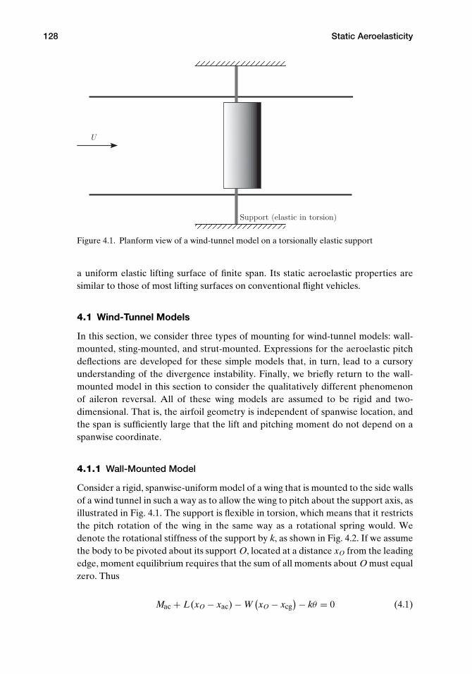
128 Static Aeroelasticity
Figure 4.1. Planform view of a wind-tunnel model on a torsionally elastic support
a uniform elastic lifting surface of finite span. Its static aeroelastic properties aresimilar to those of most lifting surfaces on conventional flight vehicles.
4.1 Wind-Tunnel Models
In this section, we consider three types of mounting for wind-tunnel models: wall-mounted, sting-mounted, and strut-mounted. Expressions for the aeroelastic pitchdeflections are developed for these simple models that, in turn, lead to a cursoryunderstanding of the divergence instability. Finally, we briefly return to the wall-mounted model in this section to consider the qualitatively different phenomenonof aileron reversal. All of these wing models are assumed to be rigid and two-dimensional. That is, the airfoil geometry is independent of spanwise location, andthe span is sufficiently large that the lift and pitching moment do not depend on aspanwise coordinate.
4.1.1 Wall-Mounted Model
Consider a rigid, spanwise-uniform model of a wing that is mounted to the side wallsof a wind tunnel in such a way as to allow the wing to pitch about the support axis, asillustrated in Fig. 4.1. The support is flexible in torsion, which means that it restrictsthe pitch rotation of the wing in the same way as a rotational spring would. Wedenote the rotational stiffness of the support by k, as shown in Fig. 4.2. If we assumethe body to be pivoted about its support O, located at a distance xO from the leadingedge, moment equilibrium requires that the sum of all moments about O must equalzero. Thus
Mac + L(xO − xac) − W(xO − xcg
)− kθ = 0 (4.1)

4.1 Wind-Tunnel Models 129
U W O
k
c
xcg
xac
xO
Macα
L
Figure 4.2. Airfoil for wind-tunnel model
Were the support rigid, the angle of attack would be αr, positive nose-up. Theelastic part of the pitch angle is denoted by θ , which is also positive nose-up. The wingangle of attack is then α ≡ αr + θ . In anticipation of using linear aerodynamics, weassume the angle of attack, α, to be a small angle, such that sin(α) ≈ α and cos(α) ≈ 1.It also is necessary to restrict the analysis to “thin” airfoils (i.e., small thickness tochord and small camber). The treatment herein is restricted to incompressible flow,but compressibility effects may be taken into account by means of Prandtl-Glauertcorrections to the airfoil coefficients. For this, the freestream Mach number mustremain less than roughly 0.8 to avoid transonic effects.
For linear aerodynamics, the lift for a rigid support is simply
Lrigid = qSCLααr (4.2)
whereas the lift for an elastic support is
L = qSCLα(αr + θ) (4.3)
where q = 12ρ∞U2 is the freestream dynamic pressure (i.e., in the far field—often
denoted by q∞), U is the freestream air speed, ρ∞ is the freestream air density, Sis the planform area, and CLα
is the wing lift-curve slope. Note that L �= Lrigid; forpositive θ , L > Lrigid. We can express the moment of aerodynamic forces about theaerodynamic center as
Mac = qScCMac (4.4)
If the angle of attack is small, CMac can be regarded as a constant. Note here thatlinear aerodynamics implies that the lift-curve slope CLα
is a constant. A furthersimplification may be that CLα
= 2π in accordance with two-dimensional thin-airfoiltheory. If experimental data or results from computational fluid dynamics providean alternative value, then it should be used.
Using Eqs. (4.3) and (4.4), the equilibrium equation, Eq. (4.1), can be expandedas
qScCMac + qSCLα(αr + θ) (xO − xac) − W
(xO − xcg
) = kθ (4.5)
130 Static Aeroelasticity
Solving Eq. (4.5) for the elastic deflection, we obtain
θ = qScCMac + qSCLααr (xO − xac) − W
(xO − xcg
)k − qSCLα
(xO − xac)(4.6)
When αr and q are specified, the total lift can be determined.When the lift acts upstream of point O, an increase in lift increases α that, in
turn, increases lift. Thus, lift is a destabilizing influence counteracting the restrainingaction of the spring when xO > xac. Recalling the discussion of stability in Section2.5, when a system is perturbed from a state of equilibrium and tends to divergefurther from its equilibrium state, we say that the system is unstable. Such is the casewhen the moment of the lift about point O exceeds the restoring moment from thespring. This is one of the simplest examples of the static aeroelastic instability called“divergence.” Now, from Eq. (4.6), we see that the aerodynamic center is forward ofthe support point O when xac < xO, making it possible for the denominator to vanishor for θ to blow up when q is sufficiently large. The denominator of the expressionfor θ is a sort of effective stiffness, which decreases as q of increases. When thedenominator vanishes, divergence occurs. The divergence dynamic pressure—ordynamic pressure at which divergence occurs—is then denoted by
qD = kSCLα
(xO − xac)(4.7)
From this, the divergence speed—or the air speed at which divergence occurs—canbe found as
UD =√
2kρ∞SCLα
(xO − xac)(4.8)
It is evident that when the aerodynamic center is coincident with the pivot, sothat xO = xac, the divergence dynamic pressure becomes infinite. Also, when theaerodynamic center is aft of the pivot so that xO < xac, the divergence dynamicpressure becomes negative. Because for physical reasons dynamic pressure must bepositive and finite, it is clear in either case that divergence is impossible.
To further pursue the character of this instability, consider the case of a symmet-ric airfoil (CMac = 0). Furthermore, let xO = xcg so that the weight term drops outof the equation for θ . From Eq. (4.7), we can let k = qDSCLα
(xO − xac); therefore,θ can be written simply as
θ = αrqDq − 1
(4.9)
The lift is proportional to αr + θ . Thus, the change in lift divided by the rigid lift isgiven by
�LLrigid
= θ
αr=
qqD
1 − qqD
(4.10)
Both θ and �L/Lrigid clearly approach infinity as q → qD. Indeed, a plot of the latteris given in Fig. 4.3 and shows the large change in lift caused by the aeroelastic effect.The lift evidently starts from its “rigid” value—that is, the value it would have were

4.1 Wind-Tunnel Models 131
0.0 0.2 0.4 0.6 0.8
q
qD
1
2
3
4
5
6
L
L rigid
Figure 4.3. Relative change in lift due to aeroelastic effect
the support rigid—and increases to infinity as q → qD. However, remember thatthere are limitations on the validity of both expressions. Namely, the lift will notcontinue to increase as stall is encountered. Moreover, because the structure will nottolerate infinite deformation, failure takes place at some finite value of θ—generallyat a dynamic pressure well below the divergence dynamic pressure.
When the system parameters are within the bounds of validity for linear theory,another fascinating feature of this problem emerges. We can invert the expressionfor θ to obtain
1θ
= qD
αr
(1q
− 1qD
)(4.11)
making it evident that 1/θ is proportional to 1/q (Fig. 4.4). Therefore, for a modelof this type, only two data points are needed to extrapolate the line down and to theleft until it intercepts the 1/q axis at a distance 1/qD from the origin. As shown inthe figure, the slope of this line also can be used to estimate qD. The form of thisplot is of great practical value because estimates of qD can be extrapolated from datataken at speeds far below the divergence speed. This means that qD can be estimatedeven when the values of the model parameters are not precisely known, therebycircumventing the need to risk destruction of the model by testing all the way up tothe divergence boundary.
4.1.2 Sting-Mounted Model
A second configuration of potential interest is a rigid model mounted on an elasticsting. A simplified version of this kind of model is shown in Figs. 4.5 through 4.7, inwhich the sting is modeled as a uniform, elastic, clamped-free beam with bending

132 Static Aeroelasticity
α
Figure 4.4. Plot of 1/θ versus 1/q
stiffness EI and length λc, where λ is a dimensionless parameter. The model ismounted in such a way as to have angle of attack of αr when the beam is undeformed.Thus, as before, α = αr + θ , where θ is the nose-up rotation of the wing resultingfrom bending of the sting, as shown in Fig. 4.6. Also in Fig. 4.6, we denote the tipdeflection of the beam as δ, although we do not need it for this analysis. Note theequal and opposite directions on the force F0 and moment M0 at the trailing edge ofthe wing in Fig. 4.7 versus at the tip of the sting in Fig. 4.6.
Figure 4.5. Schematic of a sting-mounted wind-tunnel model

4.1 Wind-Tunnel Models 133
δ
θ
Figure 4.6. Detailed view of the clamped-free beam
From superposition, we can deduce the total bending slope at the tip of the stingas the sum of contributions from the tip force F0 and tip moment M0, denoted by θF
and θM, respectively, so that
θ = θF + θM (4.12)
From elementary beam theory, these constituent parts can be written as
θF = F0(λc)2
2EI
θM = M0(λc)
EI
(4.13)
so that
F0 = 2EI θF
(λc)2
M0 = EI θM
λc
(4.14)
Two static aeroelastic equilibrium equations now can be written for the deter-mination of θF and θM. Using Eqs. (4.3) and (4.4) for the lift and pitching moment,
α-
Figure 4.7. Detailed view of the sting-mounted wing

134 Static Aeroelasticity
Figure 4.8. Schematic of strut-supported wind-tunnel model
the force equilibrium equation can be written as
qSCLα(αr + θF + θM) − W − F0 = 0 (4.15)
and the sum of moments about the trailing edge yields
qScCMac + qSCLα(αr + θF + θM) (c − xac) − W
(c − xcg
)− M0 = 0 (4.16)
Substitution of Eqs. (4.14) into Eqs. (4.15) and (4.16), simultaneous solution for θF
and θM, and use of Eq. (4.12) yields
θ =W(λ + 2 − 2rcg
)− 2qSCMac
qSCLα
− αr (λ + 2 − 2rac)
λ + 2 − 2rac − 2EIλc2qSCLα
(4.17)
where rac = xac/c and rcg = xcg/c. Here again, the condition for divergence can beobtained by setting the denominator to zero, so that
qD = 2EIc2Sλ (λ + 2 − 2rac) CLα
(4.18)
However, unlike the previous example, we cannot make the divergence dynamicpressure infinite or negative (thereby making divergence mathematically impos-sible) by choice of configuration parameters because xac/c ≤ 1. For a given wingconfiguration, we are left only with the possibility of increasing the sting’s bendingstiffness or decreasing λ to make the divergence dynamic pressure larger.
4.1.3 Strut-Mounted Model
A third configuration of a wind-tunnel mount is a strut system, as illustrated inFigs. 4.8 and 4.9. The two linearly elastic struts have the same extensional stiffness, k,and are mounted at the leading and trailing edges of the wing. The model is mountedin such a way as to have an angle of attack of αr when the springs are both unde-formed. Thus, as before, the angle of attack is α = αr + θ . As illustrated in Fig. 4.9,the elastic part of the pitch angle, θ , can be related to the extension of the two struts as
θ = δ1 − δ2
c(4.19)

4.1 Wind-Tunnel Models 135
δ δ
Figure 4.9. Cross section of strut-supported wind-tunnel model
The sum of the forces in the vertical direction shows that
L− W − k(δ1 + δ2) = 0 (4.20)
The sum of the moments about the trailing edge yields
Mac + L(c − xac) − W(c − xcg) − kcδ1 = 0 (4.21)
Again, using Eqs. (4.3) and (4.4) for the lift and pitching moment, the simultaneoussolution of the force and moment equations yields
θ =αr(1 − 2 xac
c
)+ 2 CMacCLα
− WqSCLα
(1 − 2
xcgc
)kc
qSCLα− (
1 − 2 xacc
) (4.22)
As usual, the divergence condition is indicated by the vanishing of the denominator,so that
qD = kc
SCLα
(1 − 2 xac
c
) (4.23)
It is evident for this problem as specified that when the aerodynamic center is infront of the mid-chord (as it is in subsonic flow), the divergence condition cannotbe eliminated. However, divergence can be eliminated if the leading-edge springstiffness is increased relative to that of the trailing-edge spring. This is left as anexercise for readers (see Problem 5).
4.1.4 Wall-Mounted Model for Application to Aileron Reversal
Before leaving the wind-tunnel-type models discussed so far in this chapter, weconsider the problem of aileron reversal. “Aileron reversal” is the reversal of theaileron’s expected response due to structural deformation of the wing. For exam-ple, wing torsional flexibility can cause ailerons to gradually lose their effectivenessas dynamic pressure increases; beyond a certain dynamic pressure that we call the“reversal dynamic pressure,” they start to function in a manner that is opposite totheir intended purpose. The primary danger posed by the loss of control effectiveness

136 Static Aeroelasticity
U
β
α
Figure 4.10. Schematic of the airfoil section of a flapped two-dimensional wing in a windtunnel
is that the pilot cannot control the aircraft in the usual way. There are additionalconcerns for aircraft, the missions of which depend on their being highly maneu-verable. For example, when control effectiveness is lost, the pilot may not be ableto count on the aircraft’s ability to execute evasive maneuvers. This loss in controleffectiveness and eventual reversal is the focus of this section.
Consider the airfoil section of a flapped two-dimensional wing, shown in Fig. 4.10.Similar to the model discussed in Section 4.1.1, the wing is pivoted and restrained bya rotational spring with spring constant k. The main differences are that (1) a trailing-edge flap is added such that the flap angle β can be arbitrarily set by the flight-controlsystem; and (2) we need not consider gravity to illustrate this phenomenon, so theweight is not shown in the figure. Moment equilibrium for this system about thepivot requires that
Mac + eL = kθ (4.24)
The lift and pitching moment for a two-dimensional wing can be written asbefore; namely
L = qSCL
Mac = qcSCMac(4.25)
When β �= 0, the effective camber of the airfoil changes, inducing changes in bothlift and pitching moment. For a linear theory, both α and β should be small angles,so that
CL = CLαα + CLβ
β
CMac = CM0 + CMββ
(4.26)
where, as before, the angle of attack is α = αr + θ . Note that CMβ< 0; for conve-
nience, we assume a symmetric airfoil (CM0 = 0).Note that we may most directly determine the divergence dynamic pressure by
writing the equilibrium equation without the inhomogeneous terms; that is
(k − eqSCLα)θ = 0 (4.27)

4.1 Wind-Tunnel Models 137
A nontrivial solution exists when the coefficient of θ vanishes, yielding the divergencedynamic pressure as
qD = keSCLα
(4.28)
Clearly, the divergence dynamic pressure is unaffected by the aileron.Conversely, the response is significantly affected by the aileron, as we now show.
We can solve the response problem by substituting Eqs. (4.25) into the moment-equilibrium equation, Eq. (4.24), making use of Eqs. (4.26), and determining θ
to be
θ = qS[eCLα
αr + (eCLβ
+ cCMβ
)β]
k − eqSCLα
(4.29)
We see that because of the flexibility of the model in pitch (representative of torsionalflexibility in a wing), θ is a function of β. We then find the lift as follows:
1. Substitute Eq. (4.29) into α = αr + θ to obtain α.2. Substitute α into the first of Eqs. (4.26) to obtain the lift coefficient.3. Finally, substitute the lift coefficient into the first of Eqs. (4.25) to obtain an
expression for the aeroelastic lift:
L =qS
[CLα
αr + CLβ
(1 + cqSCLα CMβ
kCLβ
)β]
1 − eqSCLα
k
(4.30)
It is evident from the two terms in the coefficient of β in this expression that lift is afunction of β in two counteracting ways. Ignoring the effect of the denominator, wesee that the first term in the numerator that multiplies β is purely aerodynamic andleads to an increase in lift with β because of a change in the effective camber. Thesecond term is aeroelastic. Recalling that CMβ
< 0, we see that as β is increased, theeffective change in the camber also induces a nose-down pitching moment that—because the model is flexible in pitch—tends to decrease θ and in turn decrease lift.At low speed, the purely aerodynamic increase in lift overpowers the aeroelastictendency to decrease the lift, so that the lift indeed increases with β (and the aileronworks as advertised). However, as dynamic pressure increases, the aeroelastic effectbecomes stronger; there is a point at which the net rate of change of lift with respectto β vanishes so that
∂L∂β
= 0 =qSCLβ
(1 + cqSCLα CMβ
kCLβ
)1 − eqSCLα
k
(4.31)
Thus, we find that the dynamic pressure at which the reversal occurs is
qR = − kCLβ
cSCLαCMβ
(4.32)
Notice that because CMβ< 0, qR > 0. Obviously, a stiffer k gives a higher reversal
speed, and a model that is rigid in pitch (analogous to a torsionally rigid wing) will

138 Static Aeroelasticity
not undergo reversal. For dynamic pressures above qR (but still below the divergencedynamic pressure), a positive β will actually decrease the lift.
Now let us consider the effect of both numerator and denominator. As discussedpreviously, the divergence dynamic pressure also can be found by setting the denom-inator of L or θ equal to zero, resulting in the same expression for qD as found inEq. (4.27). Equations (4.27) and (4.32) can be used to simplify the expression for thelift in Eq. (4.30) to obtain
L =qS
[CLα
αr + CLβ
(1 − q
qR
)β]
1 − qqD
(4.33)
It is clear from this expression that the coefficient of β can be positive, negative, orzero. Thus, a positive β could increase the lift, decrease the lift, or not change the liftat all. The aileron’s lift efficiency, η, can be thought of as the aeroelastic (i.e., actual)change in lift per unit change in β divided by the change in lift per unit change in β
that would result were the model not flexible in pitch; that is
η = change in lift per unit change in β for elastic wingchange in lift per unit change in β for rigid wing
Using this, we can easily find that
η =1 − q
qR
1 − qqD
(4.34)
which implies that the wing will remain divergence-free and control efficiency willnot be lost as long as q < qD ≤ qR. Obviously, were the model rigid in pitch, both qD
and qR would become infinite and η = 1.Thinking unconventionally for the moment, let us allow the possibility of qR �
qD. This will result in aileron reversal at a low speed, of course. Although theaileron now works opposite to the usual way at most operational speeds of theaircraft, this type of design should not be ruled out on these grounds alone. Activeflight-control systems certainly can compensate for this. Moreover, we can obtainconsiderably more (negative) lift for positive β in this unusual regime than positivelift for positive β in the more conventional setting. This concept is a part of the designof the Kaman “servo-flap rotor,” the blades of which have trailing-edge flaps that flapup for increased lift. It also may have important implications for the design of highlymaneuverable aircraft. Exactly what other potential advantages and disadvantagesexist from following this strategy—particularly in this era of composite materials,smart structures, and active controls—is not presently known and is the subject ofcurrent research.
We revisit this problem in Section 4.2.5 from the point of view of a flexible beammodel for the wing.

4.2 Uniform Lifting Surface 139
Figure 4.11. Uniform unswept clamped-free lifting surface
4.2 Uniform Lifting Surface
So far, our aeroelastic analyses focused on rigid wings with a flexible support. Theseidealized configurations provide insight into the aeroelastic stability and response,but practical analyses must take into account flexibility of the lifting surface. That be-ing the case, in this section, we address flexible wings, albeit with simplified structuralrepresentation.
Consider an unswept uniform elastic lifting surface as illustrated in Figs. 4.11and 4.12. The lifting surface is modeled as a beam and, in keeping with historicalpractice in the field of aeroelasticity, the spanwise coordinate along the elastic axisis denoted by y. The beam is presumed to be built in at the root (i.e., y = 0, torepresent attachment to a wind-tunnel wall or a fuselage) and free at the tip (i.e.,y = �). The y axis corresponds to the elastic axis, which may be defined as the line ofeffective shear centers, assumed here to be straight. Recall that for isotropic beams,a transverse force applied at any point along this axis results in bending with noelastic torsional rotation about the axis. This axis is also the axis of twist in responseto a pure twisting moment applied to the wing. Because the primary concern here

140 Static Aeroelasticity
M 'ac
Figure 4.12. Cross section of spanwise uniform lifting surface
is the determination of the airload distributions, the only elastic deformation thatinfluences these loads is rotation due to twist about the elastic axis.
4.2.1 Steady-Flow Strip Theory
In Section 4.1, wings are assumed to be rigid and two-dimensional. That is, the airfoilgeometry including incidence angle is independent of spanwise location, and thespan is sufficiently large that lift and pitching moment are not functions of a spanwisecoordinate. In turning our attention to wings that can be modeled as isotropic beams,the incidence angle now may be a function of the spanwise coordinate because of thepossibility of elastic twist. We need the distributed lift force and pitching momentper unit span exerted by aerodynamic forces along a slender beam-like wing. At thisstage, however, we ignore the three-dimensional tip effects associated with wings offinite length; the aerodynamic loads at a given spanwise location do not depend onthose at any other.
The total applied, distributed, twisting moment per unit span about the elasticaxis is denoted as M′(y), which is positive leading-edge-up and given by
M′ = M′ac + eL′ − Nmgd (4.35)
where L′ and M′ac are the distributed spanwise lift and pitching moment (i.e., the lift
and pitching moment per unit length), mg is the spanwise weight distribution (i.e.,the weight per unit length), and N is the “normal load factor” for the case in whichthe wing is level (i.e., the z axis is directed vertically upward). Thus, N can be writtenas
N = LW
= 1 + Az
g(4.36)
where Az is the z component of the wing’s inertial acceleration, W is the total weightof the aircraft, and L is the total lift.
The distributed aerodynamic loads can be written in coefficient form as
L′ = qcc�
M′ac = qc2cmac
(4.37)

4.2 Uniform Lifting Surface 141
where the freestream dynamic pressure, q, is
q = 12ρ∞U2 (4.38)
Note that the sectional lift c� and moment cmac coefficients are written here inlower case to distinguish them from lift and pitching moment coefficients for a two-dimensional wing, which are normally written in upper case. Finally, the primes areincluded with L′, M′, and M′
ac to reflect that these are distributed quantities (i.e., perunit span).
The sectional lift and pitching-moment coefficients can be related to the angle ofattack α by an appropriate aerodynamic theory as some functions c�(α) and cmac(α),where the functional relationship generally involves integration over the planform.To simplify the calculation, the wing can be broken up into spanwise segments ofinfinitesimal length, where the local lift and pitching moment can be estimated fromtwo-dimensional theory. This theory, commonly known as “strip theory,” frequentlyuses a table for efficient calculation. Here, however, for small values of α, we mayuse an even simpler form in which the lift–curve slope is assumed to be a constantalong the span, so that
c�(y) = aα(y) (4.39)
where a denotes the constant sectional lift–curve slope, and the sectional-momentcoefficient cmac(α) is assumed to be a constant along the span.
The angle of attack is represented by two components. The first is a rigid con-tribution, αr, from a rigid rotation of the surface (plus any built-in twist, althoughnone is assumed to exist here). The second component is the elastic angle of twistθ(y). Hence
α(y) = αr + θ(y) (4.40)
where, as is appropriate for strip theory, the contribution from downwash associatedwith vortices at the wing tip is neglected. Therefore, associated with the angle ofattack at each infinitesimal section is a component of sectional-lift coefficient givenby strip theory as
c�(y) = a[αr + θ(y)] (4.41)
4.2.2 Equilibrium Equation
Because we are analyzing the static behavior of this wing, it is appropriate to simplifythe fundamental constitutive relationship of torsional deformation, Eq. (2.42), toread
T = GJdθ
dy(4.42)
where GJ is the effective torsional stiffness and T is the twisting moment aboutthe elastic axis. Now, a static equation of moment equilibrium about the elastic axis

142 Static Aeroelasticity
can be obtained by equating the rate of change of twisting moment to the negativeof the applied torque distribution. This is a specialization of Eq. (2.43) in whichtime-dependent terms are ignored, yielding
dTdy
= ddy
(GJ
dθ
dy
)= −M′ (4.43)
Recognizing that uniformity implies GJ is constant over the length; substitutingEqs. (4.37) into Eq. (4.35) to obtain the applied torque; and, finally, substituting theapplied torque and Eq. (4.42) for the internal torque into the equilibrium equation,Eq. (4.43), we obtain
GJd2θ
dy2= −qc2cmac − eqcc� + Nmgd (4.44)
Eq. (4.41) now can be substituted into the equilibrium equation to yield an in-homogeneous, second-order, ordinary differential equation with constant coefficients
d2θ
dy2+ qcae
GJθ = − 1
GJ
(qc2cmac + qcaeαr − Nmgd
)(4.45)
A complete description of this equilibrium condition requires specification of theboundary conditions. Because the surface is built in at the root and free at the tip,these conditions can be written as
y = 0: θ = 0 (zero deflection)
y = �:dθ
dy= 0 (zero twisting moment)
(4.46)
Obviously, these boundary conditions are valid only for the clamped-free condition.The boundary conditions for other end conditions for beams in torsion are given inSection 3.2.2.
4.2.3 Torsional Divergence
If it is presumed that the configuration parameters of the uniform wing are known,then it is possible to solve Eq. (4.45) to determine the resulting twist distribution andassociated airload. To simplify the notation, let
λ2 ≡ qcae
GJ
λ2αr ≡ 1
GJ
(qc2cmac − Nmgd
) (4.47)
so that
αr = ccmac
ae− Nmgd
qcae(4.48)

4.2 Uniform Lifting Surface 143
Note that λ2 and αr are independent of y because the wing is assumed to be uniform.The static-aeroelastic equilibrium equation now can be written as
d2θ
dy2+ λ2θ = −λ2 (αr + αr) (4.49)
The general solution to this linear ordinary differential equation is
θ = Asin(λy) + Bcos(λy) − (αr + αr) (4.50)
subject to the condition that λ �= 0. Applying the boundary conditions, we find that
θ(0) = 0: B = αr + αr
θ ′(�) = 0: A= B tan(λ�)(4.51)
where ( )′ = d( )/dy. Thus, the elastic-twist distribution becomes
θ = (αr + αr) [tan(λ�) sin(λy) + cos(λy) − 1] (4.52)
Because θ is now known, the spanwise-lift distribution can be found using therelationship
L′ = qca(αr + θ) (4.53)
It is important to note from the expression for elastic twist that θ becomesinfinite as λ� approaches π/2. This phenomenon is called “torsional divergence” anddepends on the numerical value of
λ =√
qcae
GJ(4.54)
Thus, it is apparent that there exists a value of the dynamic pressure q = qD, at whichλ� equals π/2, where the elastic twist theoretically becomes infinite. The value qD iscalled the “divergence dynamic pressure” and is given by
qD = GJeca
( π
2�
)2(4.55)
Noting now that we can write
λ� = π
2
√q (4.56)
with
q = qqD
(4.57)
the twist angle of the wing at the tip can be written as
θ(�) = (αr + αr) [sec(λ�) − 1]
= (αr + αr)[sec
(π
2
√q)
− 1] (4.58)

144 Static Aeroelasticity
0.2 0.4 0.6 0.8 1.0q
2
4
6
8
10
θtip degrees
Figure 4.13. Plot of twist angle for the wing tip versus q for αr + αr = 1◦
where Eq. (4.48) now can be written as
αr = ccmac
ae− 4�2 Nmgd
GJπ2q(4.59)
Letting d be zero so that αr becomes independent of q, we can examine the behaviorof θ(�) versus q. Such a function is plotted in Fig. 4.13, where we see that the tip-twistangle goes to infinity as q approaches unity. Note that the character of the plot inFig. 4.13 is similar to the prebuckling behavior of columns that have imperfections.It is of practical interest to note that the tip-twist angle may become sufficiently largeto warrant concern about the structural integrity for dynamic pressures well belowqD. In practice, designers normally require the divergence dynamic pressure to beoutside of the vehicle’s flight envelope—perhaps by specifying an appropriate factorof safety.
Because this instability occurs at a dynamic pressure that is independent of theright-hand side of Eq. (4.49), as long as the right-hand side is nonzero, it seemspossible that the divergence condition could be obtained from the homogeneousequilibrium equation
d2θ
dy2+ λ2θ = 0 (4.60)
The general solution to this eigenvalue problem of the Sturm–Liouville type is
θ = Asin(λy) + Bcos(λy) (4.61)
for λ �= 0. Applying the boundary conditions, we obtain
θ(0) = 0: B = 0
θ ′(�) = 0: Aλ cos(λ�) = 0(4.62)
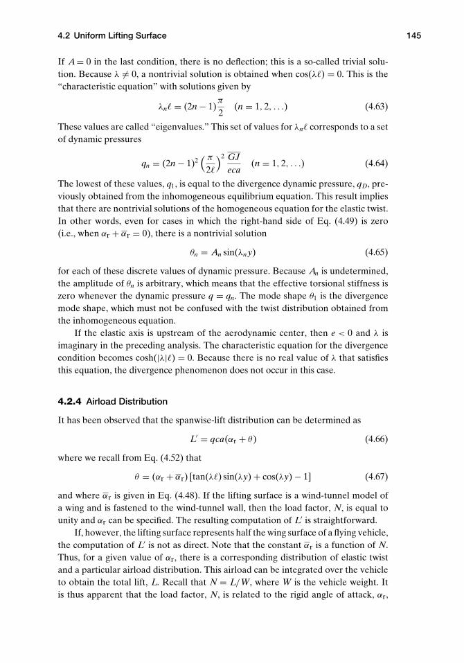
4.2 Uniform Lifting Surface 145
If A= 0 in the last condition, there is no deflection; this is a so-called trivial solu-tion. Because λ �= 0, a nontrivial solution is obtained when cos(λ�) = 0. This is the“characteristic equation” with solutions given by
λn� = (2n − 1)π
2(n = 1, 2, . . .) (4.63)
These values are called “eigenvalues.” This set of values for λn� corresponds to a setof dynamic pressures
qn = (2n − 1)2( π
2�
)2 GJeca
(n = 1, 2, . . .) (4.64)
The lowest of these values, q1, is equal to the divergence dynamic pressure, qD, pre-viously obtained from the inhomogeneous equilibrium equation. This result impliesthat there are nontrivial solutions of the homogeneous equation for the elastic twist.In other words, even for cases in which the right-hand side of Eq. (4.49) is zero(i.e., when αr + αr = 0), there is a nontrivial solution
θn = An sin(λn y) (4.65)
for each of these discrete values of dynamic pressure. Because An is undetermined,the amplitude of θn is arbitrary, which means that the effective torsional stiffness iszero whenever the dynamic pressure q = qn. The mode shape θ1 is the divergencemode shape, which must not be confused with the twist distribution obtained fromthe inhomogeneous equation.
If the elastic axis is upstream of the aerodynamic center, then e < 0 and λ isimaginary in the preceding analysis. The characteristic equation for the divergencecondition becomes cosh(|λ|�) = 0. Because there is no real value of λ that satisfiesthis equation, the divergence phenomenon does not occur in this case.
4.2.4 Airload Distribution
It has been observed that the spanwise-lift distribution can be determined as
L′ = qca(αr + θ) (4.66)
where we recall from Eq. (4.52) that
θ = (αr + αr) [tan(λ�) sin(λy) + cos(λy) − 1] (4.67)
and where αr is given in Eq. (4.48). If the lifting surface is a wind-tunnel model ofa wing and is fastened to the wind-tunnel wall, then the load factor, N, is equal tounity and αr can be specified. The resulting computation of L′ is straightforward.
If, however, the lifting surface represents half the wing surface of a flying vehicle,the computation of L′ is not as direct. Note that the constant αr is a function of N.Thus, for a given value of αr, there is a corresponding distribution of elastic twistand a particular airload distribution. This airload can be integrated over the vehicleto obtain the total lift, L. Recall that N = L/W, where W is the vehicle weight. Itis thus apparent that the load factor, N, is related to the rigid angle of attack, αr,

146 Static Aeroelasticity
through the elastic twist angle, θ . For this reason, either of the two variables αr andN can be specified; the other then can be obtained from the total lift L. Assuming atwo-winged vehicle with all the lift being generated from the wings, we find
L = 2∫ �
0L′ dy (4.68)
Substituting for L′ and αr as given herein yields
L = 2qca∫ �
0
{αr + (αr + αr) [tan(λ�) sin(λy) + cos(λy) − 1]
}dy
= 2qca�
{(αr + αr)
[tan(λ�)
λ�
]− αr
} (4.69)
Because N = L/W, this expression can be divided by the vehicle weight to yielda relationship for N in terms of αr and αr. This relationship then can be solvedsimultaneously with the preceding expression for αr, Eq. (4.48), in terms of αr andN. In this manner, αr can be eliminated, providing either a relationship that expressesN in terms of αr, given by
N =2GJ (λ�)2
{aeαr + ccmac
[1 − λ�
tan(λ�)
]}
ae�{
Weλ�tan(λ�) + 2mg�d
[1 − λ�
tan(λ�)
]} (4.70)
or a relationship that expresses αr in terms of N
αr = NW�e
2GJλ� tan(λ�)+[
1 − λ�
tan(λ�)
] [Nmg�2d
GJ (λ�)2− ccmac
ae
](4.71)
These relationships permit us to specify a constant αr and find N(q) or, alternatively,to specify a constant N and find αr(q). We find that N(q) starts out at zero for q = 0.Conversely, αr(q) starts out at infinity for q = 0. The limiting values as q → qD
depend on the other parameters. These equations can be used to find the torsionaldeformation and the resulting airload distribution for a specified flight condition.
The calculation of the spanwise aeroelastic airload distribution is immenselypractical and is used in industry in two separate ways. First, it is used to satisfy arequirement of aerodynamicists or performance engineers who need to know thetotal force and moment on the flight vehicle as a function of altitude and flightcondition. In this instance, the dynamic pressure q (and altitude or Mach number)and αr are specified, and the load factor N or total lift L is computed using Eq. (4.70).
A second requirement is that of structural engineers, who must ensure the struc-tural integrity of the lifting surface for a specified load factor N and flight condition.Such a specification normally is described by what is called a V-N diagram. Forthe conditions of given load factor and flight condition, it is necessary for structuralengineers to know the airload distribution to conduct a subsequent loads and stressanalysis. When q (and altitude or Mach number) and N are specified, αr is thendetermined from Eq. (4.71). Knowing q, αr, and N, we then use Eq. (4.48) to find αr.The torsional deformation, θ , then follows from Eq. (4.67) and the spanwise-airload

4.2 Uniform Lifting Surface 147
Figure 4.14. Rigid and elastic wing-lift distribu-tions holding αr constant
distribution follows from Eq. (4.66). From this, the distributions of torsional andbending moments along the wing can be found, leading directly to the maximumstress in the wing, generally somewhere in the root cross section.
Observe that the overall effect of torsional flexibility on the unswept liftingsurface is to significantly change the spanwise-airload distribution. This effect can beseen as the presence of the elastic part of the lift coefficient, which is proportional toθ(y). Because this elastic torsional rotation generally increases as the distance fromthe root (i.e., out along the span), so also does the resultant airload distribution.The net effect depends on whether αr or N is specified. If αr is specified, as in thecase of a wall-mounted elastic wind-tunnel model (N = 1) or as in performancecomputations, then the total lift increases with the additional load appearing in theoutboard region, as shown in Fig. 4.14.
In the other case, when N is specified by a structural engineer, the total lift (i.e.,area under L′ versus y) is unchanged, as shown in Fig. 4.15. The addition of lift inthe outboard region must be balanced by a decrease inboard. This is accomplishedby decreasing αr as the surface is made more flexible.
Figure 4.15. Rigid and elastic wing-lift distribu-tions holding total lift constant

148 Static Aeroelasticity
All of the preceding equations for torsional divergence and airload distribu-tion were based on a strip-theory aerodynamic representation. A slight numericalimprovement in their predictive capability can be obtained if the two-dimensionallift–curve slope, a, is replaced everywhere by the total (i.e., three-dimensional) lift–curve slope. Although there is little theoretical justification for this modification, italters the numerical results in the direction of the exact answer. Also, it is importantto note that the lift distributions depicted in Figs. 4.14 and 4.15 cannot be generatedwith strip-theory aerodynamics because strip theory fails to pick up the dropoff ofthe airload to zero at the wing tip caused by three-dimensional effects. An aero-dynamic theory at least as sophisticated as Prandtl’s three-dimensional lifting-linetheory must be used to capture that effect. In such a case, closed-form expressionssuch as those of Eqs. (4.70) and (4.71) cannot be obtained; instead, it is necessary touse numerical methods to find N as a function of αr or αr as a function of N.
4.2.5 Aileron Reversal
In Section 4.1.4, an example illustrating aileron reversal is presented based on a rigid,two-dimensional wing with a flexible support. In this section, we examine the samephysical phenomenon using a torsionally flexible wing model. With the geometryand boundary conditions of the uniform, torsionally flexible lifting surface as before,we can derive the reversal dynamic pressure for a clamped-free wing. Two logicalchoices are presented regarding the defining condition. One is to define reversaldynamic pressure as that dynamic pressure at which the change of total lift withrespect to the aileron deflection is equal to zero. Another equally valid definition isto define it as the dynamic pressure at which the change in root-bending moment withrespect to the aileron deflection is equal to zero. Finally, we look at the effectivenessof ailerons for roll control—often termed the “roll effectiveness”—of a simplifiedflying aircraft model.
Note that the presence of an aileron requires that we modify the sectional liftand pitching moment coefficients, so that
c� = aα + c�ββ
cmac = cmββ
(4.72)
Using these coefficients and setting αr equal to zero, the sectional lift and pitchingmoment are given by
L′ = qc(aθ + c�β
β)
M′ = eL′ + qc2cmββ
(4.73)
where we assume that the aileron extends along the entire length of the wing. As-suming the weight to have a negligible effect on the reversal condition, the modifiedversion of Eq. (4.49) is written as
d2θ
dy2+ λ2θ = −λ2ψβ (4.74)
4.2 Uniform Lifting Surface 149
where
ψ = e c�β+ c cmβ
a e(4.75)
and, as before
λ2 ≡ qcaeGJ
(4.76)
With the boundary conditions of a clamped-free beam, the solution for θ is given by
θ = −ψβ [1 − cos(λy) − sin(λy) tan(λ�)] (4.77)
The total lift for the uniform lifting surface then is obtained as
L =∫ �
0L′dy = qc�
e
[(e c�β
+ c cmβ
) tan(λ�)λ�
− c cmβ
]β (4.78)
Therefore, from the first definition of aileron reversal
∂L∂β
= 0 ⇒ tan (λ�)λ�
= ccmβ
ccmβ+ ec�β
(4.79)
which, given e/c and the sectional coefficients,1 may be solved numerically for λ�.The smallest value of λ� denoted by λ1� yields the reversal dynamic pressure as
qR = (λ1�)2GJeca�2
(4.80)
We may refine the theoretical result by considering a simplified correction fromthree-dimensional effects by use of a tip-loss factor, typically chosen as B = 0.97.Instead of obtaining the total lift by integrating the sectional lift over the entire winglength from y = 0 to y = �, we integrate only from y = 0 to y = B�.
Similarly, we may account for an aileron that does not extend over the entirelength of the wing. Suppose that the aileron starts at y = r� and extends to y = R�
with 0 ≤ r < R ≤ 1. This means that there are as many as three segments to beanalyzed. There is no inhomogeneous term for the segments between y = r� andy = R�, so instead of Eq. (4.74), we write
d2θ1
dy2+ λ2θ1 = 0 0 ≤ y ≤ r�
d2θ2
dy2+ λ2θ2 = − λ2ψβ r� ≤ y ≤ R�
d2θ3
dy2+ λ2θ3 = 0 R� ≤ y ≤ �
(4.81)
1 Estimated values of the airfoil coefficients may be obtained from experiment or from XFOIL,a computer code based on a panel method for design and analysis of subsonic isolated airfoils(see Drela, 1992).
150 Static Aeroelasticity
and obtain the resulting six arbitrary constants by imposing the six boundaryconditions
θ1(0) = 0
θ1(r�) = θ2(r�)
dθ1
dy(r�) = dθ2
dy(r�)
θ2(R�) = θ3(R�)
dθ2
dy(R�) = dθ3
dy(R�)
dθ3
dy(�) = 0
(4.82)
Calculation of the reversal dynamic pressure from the second definition (i.e., theone in terms of the root-bending-moment criterion) is left as an exercise for readers(see Problem 20).
This treatment can be generalized easily to consider the roll effectiveness ofa complete aircraft model. Similar problems can be posed in the framework ofdynamics, in which the objective is, say, to predict the angular acceleration causedby deflection of a control surface, or the time to change the orientation of the aircraftfrom one roll angle to another. Depending on the aircraft and the maneuver, it maybe necessary to consider nonlinearities. Here, however, only a static, linear treatmentis included.
Consider a rolling aircraft with unswept wings, the right half of which is shownin Fig. 4.16, with a constant roll rate denoted by p. As shown in Fig. 4.17, the wingsection has an incidence angle with respect to the freestream velocity of αr + θ(y). Ina roll maneuver with p > 0, the right wing moves upward while the left wing movesdownward. The right wing then “sees” an additional component of wind velocityequal to py perpendicular to the freestream velocity and downward. As shown inFig. 4.17, because py � U, the angle of attack is reduced from the incidence angleto αr + θ − py/U.
Some contributions to the lift and pitching moment are the same (opposite) onboth sides of the aircraft; these are referred to as symmetric (antisymmetric) com-ponents. Separate problems can be posed in terms of symmetric and antisymmetricparts, which are generally uncoupled from one another. In particular, we can treatthe roll problem as an antisymmetric problem noting that all symmetric componentscancel out in pure roll. Hence, we can discard them a priori. For example, in therelationship
α = ���0
αr + θ(y) − pyU
(4.83)
the first term, αr, drops out because of symmetry. Both θ(y) and the roll-rate termare antisymmetric because θ and β have the opposite sense across the mid-plane ofthe aircraft. The last term, which represents the increment in the angle of attack from
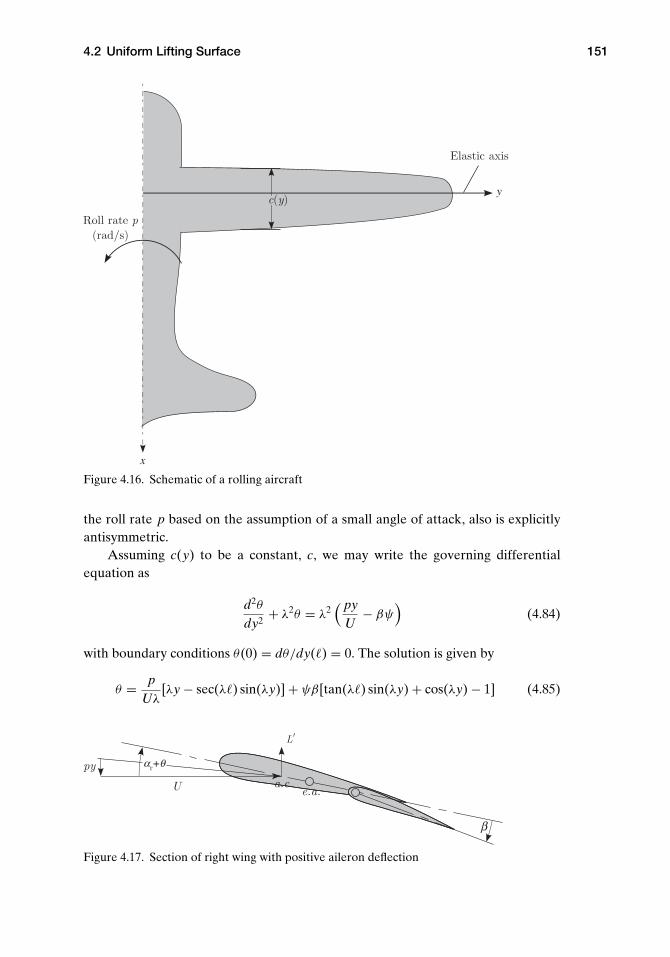
4.2 Uniform Lifting Surface 151
y
x
Figure 4.16. Schematic of a rolling aircraft
the roll rate p based on the assumption of a small angle of attack, also is explicitlyantisymmetric.
Assuming c(y) to be a constant, c, we may write the governing differentialequation as
d2θ
dy2+ λ2θ = λ2
( pyU
− βψ)
(4.84)
with boundary conditions θ(0) = dθ/dy(�) = 0. The solution is given by
θ = pUλ
[λy − sec(λ�) sin(λy)] + ψβ[tan(λ�) sin(λy) + cos(λy) − 1] (4.85)
β
α θ
Figure 4.17. Section of right wing with positive aileron deflection

152 Static Aeroelasticity
0.2 0.4 0.6 0.8 1.0λ
0.05
0.10
0.15
p
U
Figure 4.18. Roll-rate sensitivity versus λ� for e = 0.25c, c�β= 0.8, and cmβ
= −0.5, showingthe reversal point at λ� = 0.984774
Now, because the aircraft is in a steady-state rolling motion, the total rolling momentmust be equal to zero. Thus, ignoring the offset of the wing root from the mid-planeof the aircraft, we may find the moment of the lift about the mid-plane of the aircraftas ∫ �
0yL′(y)dy =
∫ �
0yqc
[a(θ − py
U
)+ c�ββ
]dy (4.86)
which, when set equal to zero, can be solved for the constant roll rate p. (Note thatthe three terms in Eq. [4.86] are the contributions toward the rolling moment dueto the elastic twist, the roll rate p, and the aileron deflection β, respectively.) Thisresult, written here in dimensionless form as p�/U, is given by
p�
U= λ�
{ccmβ
[(λ�)2 − 2 sec(λ�) + 2
]− 2ec�β[sec(λ�) − 1]
}β
2ae[λ� − tan(λ�)](4.87)
which is proportional to β. At a certain dynamic pressure, we are unable to changethe roll rate by changing β. This dynamic pressure occurs when the sensitivity of theroll rate to β vanishes; viz.
∂(
p�
U
)∂β
= λ�{ccmβ
[(λ�)2 − 2 sec(λ�) + 2
]− 2ec�β[sec(λ�) − 1]
}2ae[λ� − tan(λ�)]
= 0 (4.88)
For specific values of e/c and the sectional airfoil coefficients c�βand cmβ
, we maynumerically solve this equation for a set of roots for λ�. The lowest value is associatedthe aileron reversal. Alternatively, we simply may plot the quantity in Eq. (4.88)versus λ� until it changes sign, which is the reversal point.
For a specific case (i.e., e = 0.25c, c�β= 0.8, and cmβ
= −0.5), the roll-rate sen-sitivity is shown versus λ�, which is proportional to the speed U, in Fig. 4.18, whichshows the reversal point at λ� = 0.984774. Notice that the curve at low speed starts

4.2 Uniform Lifting Surface 153
Figure 4.19. Contributions to rolling moment R (normalized) from the three terms ofEq. (4.86)
as relatively flat and monotonically decreases until the reversal point is reached.This shape is a typical result and shows the importance of static aeroelasticity in thisaspect of flight mechanics. It is also interesting to observe the relative contributionsto the rolling moment from the elastic twist, the rolling motion, and the ailerondeflections depicted in Fig. 4.19. At the reversal point, p vanishes, and the rollingmoment contributions from elastic twist and from aileron deflection exactly cancelout one another.
4.2.6 Sweep Effects
To observe the effect of sweeping a wing aft or forward on the aeroelastic charac-teristics, it is presumed that the swept geometry is obtained by rotating the surfaceabout the root of the elastic axis, as illustrated in Fig. 4.20. The aerodynamic re-actions depend on the angle of attack as measured in the streamwise direction as
α = αr + θ (4.89)
where θ is the change in the streamwise angle of attack caused by elastic deformation.To develop a kinematical relationship for θ , we introduce the unit vectors a1 and a2,aligned with the y axis and the freestream, respectively. Another set of unit vectors,b1 and b2, is obtained by rotating a1 and a2 by the sweep angle �, as shown inFig. 4.20, so that b1 is aligned with the elastic axis (i.e., the y axis). From Fig. 4.20,we see that
b1 = cos(�)a1 + sin(�)a2
b2 = − sin(�)a1 + cos(�)a2
(4.90)
Observe that the total rotation of the local wing cross-sectional frame caused byelastic deformation can be written as the combination of rotations caused by wing

154 Static Aeroelasticity
dw
dy θ
Figure 4.20. Schematic of swept wing (positive �)
torsion, θ about b1, and wing bending, dw/dy about b2, where w is the bendingdeflection (positive up, which in Fig. 4.20 is out of the paper). Now, θ is the componentof this total rotation about a1; that is
θ =(
θ b1 + dwdy
b2
)· a1
= θ cos(�) − dwdy
sin(�)
(4.91)
From this relationship, it can be noted that as the result of sweep, the effective angleof attack is altered by bending. This coupling between bending and torsion affectsboth the static aeroelastic response of the wing in flight as well as the conditionsunder which divergence occurs. Also, it can be observed that for combined bendingand torsion of a swept, elastic wing, the section in the direction of the streamwiseairflow exhibits a change in camber—a higher-order effect that is here neglected.
To facilitate direct comparison with the previous unswept results, to the extentpossible, the same structural and aerodynamic notation is retained as was used forthe unswept planform. To determine the total elastic deflection, two equilibriumequations are required: one for torsional moment equilibrium as in the unswept caseand one for transverse force equilibrium (associated with bending). These equationscan be written as
ddy
(GJ
dθ
dy
)= −qecaα − qc2cmac + Nmgd
d2
dy2
(EI
d2w
dy2
)= qcaα − Nmg
(4.92)

4.2 Uniform Lifting Surface 155
In these equilibrium equations, a is used to denote the two-dimensional lift–curveslope of the swept surface and cmac to represent the two-dimensional pitching-moment coefficient of the swept surface. These aerodynamic constants are relatedto their unswept counterparts by
a = a cos(�)
cmac = cmac cos2(�)(4.93)
for moderate- to high-aspect-ratio surfaces. Substituting for a, α = αr + θ and, inturn, the dependence of θ on θ and w from Eq. (4.91), specializing for spanwiseuniformity so that GJ and EI are constants, and letting ( )′ denote d( )/dy, weobtain two coupled, ordinary differential equations for torsion and bending given by
θ′′ + qeca
GJθ cos2(�) − qeca
GJw′ sin(�) cos(�)
= − 1
GJ
[qecaαr cos(�) + qc2cmac cos2(�) − Nmgd
]w′′′′ + qca
EIw′ sin(�) cos(�) − qca
EIθ cos2(�) = 1
EI[qcaαr cos(�) − Nmg] (4.94)
Because the surface is built in at the root and free at the tip, the following boundaryconditions must be imposed on the solution:
y = 0: θ = 0 (zero torsional rotation)w = 0 (zero deflection)w′ = 0 (zero bending slope)
y = �: θ′ = 0 (zero twisting moment)
w′′ = 0 (zero bending moment)w′′′ = 0 (zero shear force)
(4.95)
Bending-torsion coupling is exhibited in Eqs. (4.94) through the term involving w inthe torsion equation and through the term involving θ in the bending equation.
There are two special cases of interest in which the coupling either vanishes oris much simplified so that we can solve the equations analytically. The first is for thecase of vanishing sweep in which the uncoupled torsion equation (i.e., the first ofEqs. [4.94]) is the same as previously discussed and clearly leads to solutions foreither the torsional divergence condition or the torsional deformation and air-load distribution as discussed (see Sections 4.2.3 and 4.2.4, respectively). In thelatter case, once the torsional deformation is obtained, the solution for θ = θ canbe substituted into the bending equation (i.e., the second of Eqs. [4.94]). Integra-tion of the resulting ordinary differential equation and application of the boundaryconditions lead to the shear force, bending moment, bending slope, and bendingdeflection.
A second special case occurs when e = 0. In this case, torsional divergence doesnot take place, and a polynomial solution for θ can be found from the θ equation andboundary conditions. Substitution of this solution into the bending equation leads

156 Static Aeroelasticity
ΛFigure 4.21. Divergence dynamic pressure versus �
to a fourth-order, ordinary differential equation for w with a polynomial forcingfunction; note that the θ terms are now part of that forcing function. This equationand accompanying boundary conditions can be solved for the bending deflection,but the solution is not straightforward. Alternatively, to solve this equation for adivergence condition, we need only the homogeneous part, which can be written asa third-order equation in ζ = w′; namely
ζ ′′′ + qca
EIζ sin(�) cos(�) = 0 (4.96)
For the clamped-free boundary conditions ζ (0) = ζ ′(�) = ζ ′′(�) = 0, this equationhas a known analytical solution that yields a divergence dynamic pressure of
qD = −6.32970EI
ac�3 sin(�) cos(�)(4.97)
The minus sign implies that this bending-divergence instability takes place only forforward-swept wings; that is, where � < 0.
Examination of Eqs. (4.94) illustrates that there are two ways in which the sweepinfluences the aeroelastic behavior. One way is the loss of aerodynamic effectiveness,as exhibited by the change in the second term of the torsion equations from
qeca
GJθ to
qeca
GJθ cos2(�) (4.98)
Note that this effect is independent of the direction of sweep. The second effectis the influence of bending slope on the effective angle of attack (see Eq. 4.91),which leads to bending-torsion coupling. This coupling has a strong influence onboth divergence and load distribution. The total effect of sweep depends stronglyon whether the surface is swept backward or forward. This can be illustrated by itsinfluence on the divergence dynamic pressure, qD, as shown in Fig. 4.21. It is apparentthat forward sweep causes the surface to be more susceptible to divergence, whereasbackward sweep increases the divergence dynamic pressure. Indeed, a small amountof backward sweep (i.e., for the idealized case under consideration, depending one/� and GJ/EI , only 5 or 10 degrees) can cause the divergence dynamic pressureto become sufficiently large that it ceases to be an issue. Specific cases are discussedlater in this section in conjunction with an approximate solution of the governingequations.

4.2 Uniform Lifting Surface 157
Λ
Λ>
Λ<Figure 4.22. Lift distribution for positive, zero,and negative �
The overall effect of sweep on the aeroelastic-load distribution also stronglydepends on whether the surface is swept forward or backward. This is illustrated inFig. 4.22, which shows spanwise load distributions for an elastic surface for which thetotal lift (or N) is held constant by adjusting αr. From the standpoint of structuralloads, it is apparent that the root bending moment is significantly greater for forwardsweep than for backward sweep at a given value of total lift.
The primary motivation for sweeping a lifting surface is to improve the vehicleperformance through drag reduction, although some loss in lifting capability may beexperienced. However, these aeroelastic considerations can have a significant impacton design decisions. From an aeroelastic standpoint, forward sweep exacerbatesdivergence instability and increases structural loads, whereas backward sweep canalleviate these concerns. The advent of composite lifting surfaces enabled the useof bending-twist elastic coupling to passively stabilize forward sweep, making itpossible to use forward-swept wings. Indeed, the X-29 could not have been flownwithout a means to stabilize the wings against divergence. We discuss this further inSection 4.2.7.
Exact Solution for Bending-Torsion Divergence. Extraction of the analytical solu-tion of the set of coupled, ordinary differential equations in Eqs. (4.94) is compli-cated. The exact analytical solution is obtained most easily by first converting thecoupled set of equations into a single equation governing the elastic component ofthe angle of attack. For calculation of only the divergence dynamic pressure, we canconsider just the homogeneous parts of Eqs. (4.94):
θ′′ + qeca
GJθ cos2(�) − qeca
GJw′ sin(�) cos(�) = 0
w′′′′ + qca
EIw′ sin(�) cos(�) − qca
EIθ cos2(�) = 0
(4.99)
To obtain a single equation, we differentiate the first equation with respect to y andmultiply it by cos(�). From this modified first equation, we subtract sin(�) times the
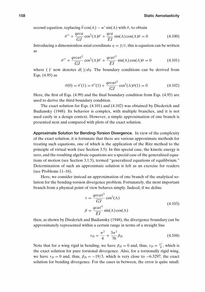
158 Static Aeroelasticity
second equation, replacing θ cos(�) − w′ sin(�) with θ , to obtain
θ ′′′ + qeca
GJcos2(�)θ ′ + qca
EIsin(�) cos(�)θ = 0 (4.100)
Introducing a dimensionless axial coordinate η = y/�, this is equation can be writtenas
θ ′′′ + qeca�2
GJcos2(�)θ ′ + qca�3
EIsin(�) cos(�)θ = 0 (4.101)
where ( )′ now denotes d( )/dη. The boundary conditions can be derived fromEqs. (4.95) as
θ(0) = θ ′(1) = θ ′′(1) + qeca�2
GJcos2(�)θ(1) = 0 (4.102)
Here, the first of Eqs. (4.99) and the final boundary condition from Eqs. (4.95) areused to derive the third boundary condition.
The exact solution for Eqs. (4.101) and (4.102) was obtained by Diederich andBudiansky (1948). Its behavior is complex, with multiple branches, and it is notused easily in a design context. However, a simple approximation of one branch ispresented next and compared with plots of the exact solution.
Approximate Solution for Bending-Torsion Divergence. In view of the complexityof the exact solution, it is fortunate that there are various approximate methods fortreating such equations, one of which is the application of the Ritz method to theprinciple of virtual work (see Section 3.5). In this special case, the kinetic energy iszero, and the resulting algebraic equations are a special case of the generalized equa-tions of motion (see Section 3.1.5), termed “generalized equations of equilibrium.”Determination of such an approximate solution is left as an exercise for readers(see Problems 11–16).
Here, we consider instead an approximation of one branch of the analytical so-lution for the bending-torsion divergence problem. Fortunately, the most importantbranch from a physical point of view behaves simply. Indeed, if we define
τ = qeca�2
GJcos2(�)
β = qca�3
EIsin(�) cos(�)
(4.103)
then, as shown by Diederich and Budiansky (1948), the divergence boundary can beapproximately represented within a certain range in terms of a straight line
τD = π2
4+ 3π2
76βD (4.104)
Note that for a wing rigid in bending, we have βD = 0 and, thus, τD = π2
4 , which isthe exact solution for pure torsional divergence. Also, for a torsionally rigid wing,we have τD = 0 and, thus, βD = −19/3, which is very close to −6.3297, the exactsolution for bending divergence. For the cases in between, the error is quite small.

4.2 Uniform Lifting Surface 159
30 20 10 10 20 30βD
10
10
20
30
40
50
60
τD
Figure 4.23. τD versus βD for coupled bending-torsion divergence; solid lines (exact solution)and dashed line (Eq. 4.104)
It is important to note that the sign of τ is driven by the sign of e, whereas the sign ofβ is driven by the sign of �. The approximate solution in Eq. (4.104) is plotted alongwith some branches of the exact solution in Fig. 4.23. Note the excellent agreementbetween the straight-line approximation and the exact solution near the origin. Notealso that the intersections of the solution with the τD axis (where βD = 0) coincidewith the squares of the roots previously obtained in Section 4.2.3, Eq. (4.63), as(2n − 1)2π2/4 for n = 1, 2, . . . , ∞ (i.e., π2/4, 9π2/4, . . .).
A more convenient way of depicting the behavior of the divergence dynamicpressure is to plot τD versus a parameter that depends on only the configuration.This can be accomplished by introducing the dimensionless parameter r , given by
r ≡ β
τ= �
eGJ
EItan(�) (4.105)
which can be positive, negative, or zero. Equation (4.104) can then be written as
τD = π2
4+ 3π2r
76τD (4.106)
Thus, we can solve for τD such that
τD = π2
4(
1 − 3π2r76
) (4.107)
or alternatively for qD, equal to
qD = GJπ2
4eca�2 cos2(�)[1 − 3π2
76�e
GJEI
tan(�)] (4.108)
Several branches of the exact solution of Eqs. (4.101) and (4.102) for the smallestabsolute values of τD versus r are plotted as solid lines in Fig. 4.24. Note that there is

160 Static Aeroelasticity
10 5 5 10r
250
200
150
100
50
50
100
D
Figure 4.24. τD versus r for coupled bending-torsion divergence; solid lines (exact solution)and dashed lines (Eq. 4.107 and τD = −27r 2/4 in fourth quadrant)
at least one branch in all quadrants except the third, and there is only one branch inthe fourth quadrant. The approximate solutions for τD versus r from Eq. (4.107) areplotted as dashed hyperbolae in the first, second, and fourth quadrants. Moreover,as r becomes large, the solution in the fourth quadrant asymptotically approachesthe parabola τD = −27r2/4, also shown as a dashed curve. Note that as in Fig. 4.23,the intersections of the roots with the τD axis are π2/4, 9π2/4, 25π2/4, and so on. Theconfiguration of any wing fixes the value of r . For positive e, we consider only positivevalues of τD. Thus, we start from zero and proceed in the positive τD direction onthis plot (i.e., at constant r) to find the first intersection with a solid line. This valueof τD is the normalized dynamic pressure at which divergence occurs. In Fig. 4.25,
10 5 5 10r
10
7.5
5
2.5
2.5
5
7.5
10D
Figure 4.25. τD versus r for coupled bending-torsion divergence; solid lines (exact solution)and dashed lines (Eq. 4.107)

4.2 Uniform Lifting Surface 161
an enlargement of these results in a more practical range is shown. It is easily seenthat the dashed lines in the first and second quadrants are close to the solid lineswhen r < 1.5. Note that when e < 0, a negative value of τD leads to a positive valueof qD. In this case, we should proceed along a line of constant r in the negative τD
direction.It is interesting that the approximate solution, despite its proximity to the exact
solution, exhibits a qualitatively different behavior mathematically. The approximatesolution exhibits an asymptotic behavior, with τD tending to plus infinity from theleft and to minus infinity from the right at the value of r that causes the denominatorto vanish—namely, when r = 76/(3π2) = 2.56680. If the approximate solution wereexact, mathematically it would mean that divergence is not possible at that valueof r . Moreover, physically it would mean that divergence is not possible for e > 0and r ≥ 76/(3π2) [or for e < 0 and r ≤ 76/(3π2)]. Actually, however, the exactsolution exhibits an instability of the “limit-point” variety. For e > 0, this means thatdivergence occurs for small and positive values of r . Moreover, as r is increased in thefirst quadrant, τD also increases until a certain point is reached, at which two thingshappen: (1) above this value of τD, the curve turns back to the left instead of reachingan asymptote; and (2) any slight increase in r beyond this point causes the solutionto jump to a higher branch. This point is called a limit point. On the main branchof the curve in the first quadrant, for example, the limit point is at r = 1.59768 andτD = 10.7090. It is shown in the plot in Fig. 4.24 that any slight increase in r causesthe solution to jump from the lower branch—where its value is 10.7090—to a higherbranch, where its value is 66.8133, at which point τD is rapidly increasing with r . So,although there is no value of r that results in an infinite exact value of the divergencedynamic pressure, practically speaking, divergence in the vicinity of the limit-pointvalue of r is all but eliminated. Thus, it is sufficient for practical purposes to say thatdivergence is not possible near those points where the approximate solution blowsup, and we may regard the approximate solution as sufficiently close to the exactsolution for design purposes. The limit point in the fourth quadrant is appropriatefor the situation in which e < 0—namely, when the aerodynamic center is behindthe elastic axis. There, the exact limit point is at r = 3.56595 and τD = −14.8345.Note that the negative values of e and τD yield a positive qD. It is left to readers asan exercise to explore this possibility further (see Problem 18).
Although there are qualitative differences, as noted, between the exact and ap-proximate solutions, within the practical range of interest, this linear approximationof the divergence boundary in terms of τD and βD is numerically accurate and leadsto a simple expression for the divergence dynamic pressure in terms of the structuralstiffnesses, e/�, and the sweep angle (i.e., Eq. [4.108]). This approximate formulacan be used in design to explore the behavior of the divergence dynamic pressureas a function of the various configuration parameters therein. For the purpose ofdisplaying results for the divergence dynamic pressure when e > 0, it is convenientto normalize qD with its value at zero sweep angle; namely
qD0 = π2GJ4eca�2
(4.109)

162 Static Aeroelasticity
Figure 4.26. Normalized divergence dynamic pres-sure for an elastically uncoupled, swept wing withGJ/EI = 1.0 and e/� = 0.02
so thatqD
qD0
= 1 + tan2(�)
1 − 3π2
76�e
GJEI
tan(�)(4.110)
Thus, for a wing structural design with given values of e, GJ , EI, and �, there arevalues of sweep angle � for which the divergence dynamic pressure goes to infinityor becomes negative, implying that divergence is not possible at those values of �.Some values of � make the numerator infinite because tan(�) blows up, whereasother values make the denominator vanish or switch signs. Therefore, within theprincipal range of −90◦ ≤ � ≤ 90◦, we can surmise that divergence can take placeonly for cases in which |�| �= 90◦ and 3π2r �= 76. Sign changes have the followingconsequences: Divergence is possible only if −90◦ < � < �∞, where
tan (�∞) = 76EIe
3π2GJ�(4.111)
Thus, Eq. (4.110) can be written as
qD
qD0
= 1 + tan2 (�)
1 − tan(�)tan(�∞)
(4.112)
In other words, we avoid divergence by choosing � ≥ �∞, and the divergence dy-namic pressure drops drastically as � is decreased below �∞. Because �∞ is likely tobe small, this frequently means that backswept wings are free of divergence and thatdivergence dynamic pressure drops drastically for forward-swept wings. Because �∞is the asymptotic value of � from the approximate solution, which is greater thanthe limit-point value of � from the exact solution, we may surmise that the approx-imate solution provides a conservative design. Figure 4.26 shows the behavior ofdivergence dynamic pressure for a wing with GJ/EI = 1.0 and e/� = 0.02. The plot,as expected, passes through unity when the sweep angle is zero. Because �∞ is verysmall for this case, the divergence dynamic pressure goes to infinity for a very smallpositive value of sweep angle. Thus, even a small angle of backward sweep can makedivergence impossible. Figure 4.27 shows the result of decreasing GJ/EI to 0.2 andholding e/� constant. Because �∞ increases, the wing must be swept back fartherthan in the previous case to avoid divergence.

4.2 Uniform Lifting Surface 163
Figure 4.27. Normalized divergence dynamic pres-sure for an elastically uncoupled, swept wing withGJ/EI = 0.2 and e/� = 0.02
Because e can be positive, negative, or zero, qD0 also may be positive, negative,or zero. Thus, by normalizing qD by qD0 , we may obfuscate the role of the sign of eon qD. In such cases and perhaps others, it is more convenient to write Eq. (4.112)in a form that does not depend on qD0 . One way to accomplish this is to eliminateqD0 from the expression for qD using Eqs. (4.109) and (4.111), yielding
qDac�3
EI= 19
[1 + tan2 (�)
]3 [tan(�∞) − tan(�)]
(4.113)
making it clearer that divergence occurs only when −90◦ < � < �∞, regardless ofthe sign of e. This form of the formula also shows more explicitly that EI has a rolein the design of swept wings that are free of divergence.
4.2.7 Composite Wings and Aeroelastic Tailoring
Aeroelastic tailoring is the design of wings using the directional properties of com-posite materials to optimize aeroelastic performance. The concept of aeroelastictailoring is relatively new and came into the forefront during the design of forward-swept wings in the 1980s. Equation (4.112) shows that qD drops dramatically forforward-swept, untailored wings. The low divergence speed was a major hurdle inthe design of wings with forward sweep. As discussed in this section, use of compos-ite materials can help remove the disadvantages of forward sweep. Currently, aero-elastic tailoring is an integral part of the design of composite wings and can be usedto improve performance in a variety of ways.
Composite materials are anisotropic, which implies different material charac-teristics (e.g., stiffness) in different directions. A simple beam model is helpful indeveloping an understanding of the behavior of composite wings. Such models mayexhibit bending-torsion elastic coupling. Analysis of beams with elastic coupling ismore involved, but it leads to helpful results.
Let us introduce such coupling in our beam equations. For anisotropic beamswith bending-torsion coupling, the “constitutive law” (i.e., the relationship between

164 Static Aeroelasticity
cross-sectional stress resultants and the generalized strains) changes from{TM
}=[
GJ 00 EI
]{θ
′
w′′
}(4.114)
to {TM
}=[
GJ −K−K EI
]{θ
′
w′′
}(4.115)
where K is the bending-torsion coupling stiffness (with the same dimensions as EIand GJ ) and ( )′ indicates the derivative with respect to y. A positive value of Kmeans that a positive bending deflection will be accompanied by a nose-up twist ofthe wing, which is normally destabilizing for cases with the elastic axis behind theaerodynamic center.
Using the coupled constitutive law, the equations of equilibrium become(GJθ
′ − Kw′′)′
= − qecaα − qc2cmac + Nmgd(EIw′′ − Kθ
′)′′= qcaα − Nmg
(4.116)
Consider again a wing that is clamped at the root and free at the tip, so that theboundary conditions that must be imposed on the solution are
y = 0: θ = 0 (zero torsional rotation)w = 0 (zero deflection)w′ = 0 (zero bending slope)
y = �: T = 0 (zero twisting moment)M = 0 (zero bending moment)M′ = 0 (zero shear force)
(4.117)
For composite beams, the offsets d and e may be defined in a manner similarto the way they were defined for isotropic beams: d is the distance from the y axisto the cross-sectional mass centroid, positive when the mass centroid is toward theleading edge from the y axis; and e is the distance from the y axis to the aerodynamiccenter, positive when the aerodynamic center is toward the leading edge from the yaxis. Recall that for composite beams, the y axis must have different properties fromthose it has for isotropic beams, and the term “elastic axis” has a different meaning.For a spanwise uniform isotropic beam, the elastic axis is along the y axis and isthe locus of cross-sectional shear centers; transverse forces acting through this axisdo not twist the beam. For spanwise uniform composite beams with bending-twistcoupling, no axis can be defined as the locus of a cross-sectional property throughwhich transverse shear forces can act without twisting the beam. For such beams, wemust place the y axis along the locus of shear centers, a point in the cross section atwhich transverse shear forces are structurally decoupled from the twisting moment.Although transverse shear forces acting at the y axis do not directly induce twist, thebending moment induced by the shear force still induces twist when K �= 0.

4.2 Uniform Lifting Surface 165
We can now write the homogeneous part of the equations of equilibrium as
θ′′ − K
GJw′′′ + qeca
GJθ cos(�) = 0
w′′′′ − K
EIθ
′′′ − qca
EIθ cos(�) = 0
(4.118)
Differentiating the first equation with respect to y and transforming the set of equa-tions so that they are uncoupled in the highest derivative terms θ
′′′and w′′′′, we
obtain
θ′′′ + EI GJ
EI GJ − K2
qeca
GJθ ′ cos(�) − K EI
EI GJ − K2
qca
EIθ cos(�) = 0
w′′′′ + K GJ
EI GJ − K2
qeca
GJθ ′ cos(�) − EI GJ
EI GJ − K2
qca
EIθ cos(�) = 0
(4.119)
Multiplying the first equation by cos(�) and the second equation by sin(�) andsubtracting the second equation from the first, we obtain a single equation in termsof θ = θ cos(�) − w′ sin(�) as
θ ′′′ + EI GJ
EI GJ − K2
qeca�2
GJcos2(�)
[1 − K
EItan(�)
]θ ′
+ EI GJ
EI GJ − K2
qca�3
EIsin(�) cos(�)
[1 − K
GJ
1tan(�)
]θ = 0
(4.120)
where ( )′ now denotes d( )/dη as in the parallel development for the elasticallyuncoupled wing discribed previously.
The boundary conditions can be derived from Eqs. (4.117) as
θ(0) = θ ′(1) = θ ′′(1) + EI GJ
EI GJ − K2
qeca�2
GJcos2(�)
[1 − K
EItan(�)
]θ(1) = 0
(4.121)
The aeroelastic divergence problem with structural coupling has the same math-ematical form as the problem without coupling, an approximate solution of whichis given in the previous section. We can see that the parameters τ and β can beredefined as
τ = EI GJ
EI GJ − K2
qeca�2
GJcos2(�)
[1 − K
EItan(�)
]
β = EI GJ
EI GJ − K2
qca�3
EIsin(�) cos(�)
[1 − K
GJ
1tan(�)
] (4.122)
and, again, the divergence boundary can be expressed approximately in terms of theline
τD = π2
4+ 3π2
76βD (4.123)

166 Static Aeroelasticity
Using the expressions for the parameters in the equation of the divergence boundary,we have
qD = π2
4EI GJ − K2
EI GJ
GJeca�2 cos2(�)
1{1 − K
EItan(�) − 3π2
76�e
GJEI
[tan(�) − K
GJ
]}(4.124)
We can simplify this by introducing the dimensionless parameter
κ = K√EI GJ
(4.125)
so that
qD = π2GJ (1 − κ2)
4eca�2 cos2(�){
1 − κ
√GJEI
tan(�) − 3π2
76�e
GJEI
[tan(�) − κ
√EIGJ
]} (4.126)
With Eq. (4.126), we may determine the divergence dynamic pressure with sufficientaccuracy to ascertain its trends versus sweep angle � and elastic-coupling parameterκ . The formula shows that there is a strong relationship between these two quantities.
To illustrate the utility of this analysis, let us first normalize qD with the value itwould have at zero sweep angle and zero coupling—namely, qD0 , so that
qD
qD0
= (1 − κ2)[1 + tan2(�)
]1 − κ
√GJEI
tan(�) − 3π2
76�e
GJEI
[tan(�) − κ
√EIGJ
] (4.127)
As before, when the denominator of the expression for divergence dynamic pres-sure vanishes, it corresponds to infinite divergence dynamic pressure; crossing this“boundary” means crossing from a regime in which divergence occurs to one inwhich it does not. Setting the denominator to zero and solving for the tangent of thesweep angle, we obtain
tan(�∞) =1 + 3π2
76
√GJEI
�e κ
3π2
76GJEI
�e +
√GJEI
κ
(4.128)
where �∞ is the sweep angle at which the divergence dynamic pressure goes toinfinity. With this definition, we can rewrite Eq. (4.127) as
qD
qD0
= (1 − κ2)[1 + tan2(�)
](
1 + 3π2
76
√GJEI
�e κ
) [1 − tan(�)
tan(�∞)
] (4.129)
Again, divergence is possible only if −90◦ < � < �∞. Thus, because of the presenceof κ as an additional design parameter, designers can at least partially compensatefor the destabilizing effect of forward sweep by appropriately choosing κ < 0, whichfor an increment of upward bending of the wing provides an increment of nose-downtwisting. There is a limit to how much coupling can be achieved, however, becausetypically |κ| < 0.86.
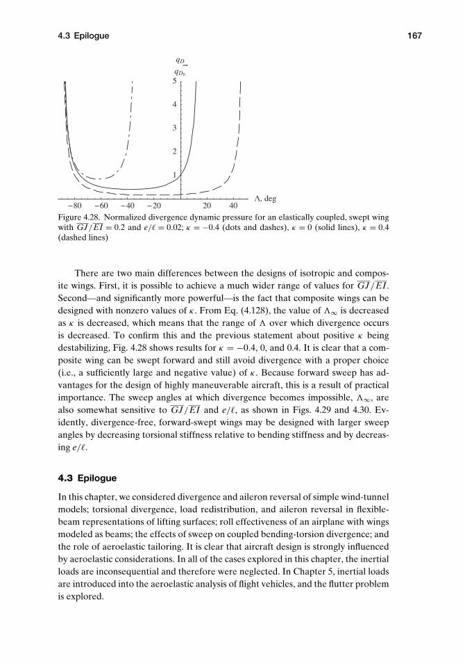
4.3 Epilogue 167
Figure 4.28. Normalized divergence dynamic pressure for an elastically coupled, swept wingwith GJ/EI = 0.2 and e/� = 0.02; κ = −0.4 (dots and dashes), κ = 0 (solid lines), κ = 0.4(dashed lines)
There are two main differences between the designs of isotropic and compos-ite wings. First, it is possible to achieve a much wider range of values for GJ/EI .Second—and significantly more powerful—is the fact that composite wings can bedesigned with nonzero values of κ . From Eq. (4.128), the value of �∞ is decreasedas κ is decreased, which means that the range of � over which divergence occursis decreased. To confirm this and the previous statement about positive κ beingdestabilizing, Fig. 4.28 shows results for κ = −0.4, 0, and 0.4. It is clear that a com-posite wing can be swept forward and still avoid divergence with a proper choice(i.e., a sufficiently large and negative value) of κ . Because forward sweep has ad-vantages for the design of highly maneuverable aircraft, this is a result of practicalimportance. The sweep angles at which divergence becomes impossible, �∞, arealso somewhat sensitive to GJ/EI and e/�, as shown in Figs. 4.29 and 4.30. Ev-idently, divergence-free, forward-swept wings may be designed with larger sweepangles by decreasing torsional stiffness relative to bending stiffness and by decreas-ing e/�.
4.3 Epilogue
In this chapter, we considered divergence and aileron reversal of simple wind-tunnelmodels; torsional divergence, load redistribution, and aileron reversal in flexible-beam representations of lifting surfaces; roll effectiveness of an airplane with wingsmodeled as beams; the effects of sweep on coupled bending-torsion divergence; andthe role of aeroelastic tailoring. It is clear that aircraft design is strongly influencedby aeroelastic considerations. In all of the cases explored in this chapter, the inertialloads are inconsequential and therefore were neglected. In Chapter 5, inertial loadsare introduced into the aeroelastic analysis of flight vehicles, and the flutter problemis explored.

168 Static Aeroelasticity
0.4 0.2 0.2 0.4κ
30
20
10
10
20
30
40
Figure 4.29. Sweep angle for which divergence dynamic pressure is infinite for a wing withGJ/EI = 0.5; solid line is for e/� = 0.01; dashed line is for e/� = 0.04
Problems
1. Consider a rigid, wind-tunnel model of a uniform wing, which is pivoted inpitch about the mid-chord and elastically restrained in pitch by a linear springwith spring constant of 225 lb/in mounted at the trailing edge. The model has asymmetric airfoil, a span of 3 feet, and a chord of 6 inches. The total lift–curve
0.4 0.2 0.2 0.4κ
40
20
20
40
Figure 4.30. Sweep angle for which divergence dynamic pressure is infinite for a wing withe/� = 0.02; solid line is for GJ/EI = 1.0; dashed line is for GJ/EI = 0.25

Problems 1–7 169
slope is 6 per rad. The aerodynamic center is located at the quarter-chord, andthe mass centroid is at the mid-chord.(a) Calculate the divergence dynamic pressure at sea level.(b) Calculate the divergence airspeed at sea level.
Answers: qD = 150 lb/ft2; UD = 355 ft/sec
2. For the model in Problem 1, for a dynamic pressure of 30 lb/ft2, compute thepercentage change in lift caused by the aeroelastic effect.Answer: 25%
3. For the model of Problem 1, propose design changes in the support system thatwould double the divergence dynamic pressure by(a) changing the stiffness of the restraining spring(b) relocating the pivot point
Answers: (a) k = 450 lb/in; (b) xO = 2.513 in
4. For the model of Problem 1 as altered by the design changes of Problem 3,calculate the percentage change in lift caused by the aeroelastic effect for adynamic pressure of 30 lb/ft2, a weight of 3 lb, αr = 0.5◦, and for(a) the design change of Problem 3a(b) the design change of Problem 3b
Answers: 11.11%; 17.91%
5. Consider a strut-mounted wing similar to the one discussed in Section 4.1.3,except that the two springs may have different stiffnesses. Denoting the leading-edge spring constant by k1 and the trailing-edge spring constant by k2, and assum-ing that the aerodynamic center is at the quarter-chord, show that divergencecan be eliminated if k1/k2 ≥ 3.
6. Using Excel or a similar tool, plot a family of curves that depict the relationship ofthe aileron-elastic efficiency, η, versus normalized dynamic pressure, q = q/qD,for various values of R = qR/qD and 0 < q < 1. Make two plots on the followingscales to reduce confusion:(a) Plot R < 1 using axes −3 < η < 3(b) Plot R > 1 using axes −3 < η < 3
Hint: Do not compute values for the cases in which 1 < R < 1.1; Excel does nothandle these well and you may get confused. For some cases, you may want toplot symbols only and nicely sketch the lines that form the curves.
Answer the following questions: Where does aileron reversal occur? If you hadto design a wing, what R would you try to match (or approach) and why? Whathappens when qR = qD? How does the efficiency change as q approaches qR?Why do you think this happens? What other pertinent features can you extractfrom these plots? Explain how you came to these conclusions.
7. Consider a torsionally elastic (GJ = 8,000 lb in2) wind-tunnel model of a uni-form wing, the ends of which are rigidly fastened to the wind-tunnel walls.The model has a symmetric airfoil, a span of 3 feet, and a chord of 6 inches.

170 Static Aeroelasticity
The sectional lift-curve slope is 6 per rad. The aerodynamic center is locatedat the quarter-chord, and both the mass centroid and the elastic axis are at themid-chord.(a) Calculate the divergence dynamic pressure at sea level.(b) Calculate the divergence airspeed at sea level.
Answers: (a) qD = 162.46 lb/ft2; (b) UD = 369.65 ft/sec
8. For the model in Problem 7, propose design changes in the model that woulddouble the divergence dynamic pressure by(a) changing the torsional stiffness of the wing(b) relocating the elastic axis
Answers: GJ = 16,000 lb in2; xea = 2.25 in
9. For the model of Problem 7, for a dynamic pressure of 30 lb/ft2, compute thepercentage increase in the sectional lift at mid-span caused by the aeroelasticeffect.Answer: 28.09%
10. For the model in Problem 7, for a dynamic pressure of 30 lb/ft2, compute thepercentage increase in the total lift caused by the aeroelastic effect.Answer: 18.58%
11. Consider a swept clamped-free wing, as described in Section 4.2.6. The governingpartial differential equations are given in Eqs. (4.94) and the boundary condi-tions in Eqs. (4.95). An approximate solution is sought for a wing with a symmet-ric airfoil, using a truncated set of assumed modes and the generalized equationsof equilibrium: a specialized version of the generalized equations of motion forwhich all time-dependent terms are zero. Note that what is being asked for hereis equivalent to the application of the Ritz method to the principle of virtualwork (see Section 3.5). With the wing weight ignored, only structural and aero-dynamic terms are involved. The structural terms of the generalized equations ofequilibrium are based on the potential energy (here, the strain energy) given by
P = 12
∫ �
0
(EIw′′2 − 2Kw′′θ
′ + GJ θ′2)
dy
and the bending and torsion deformation is represented in terms of a truncatedseries, such that
w =Nw∑i=1
ηi�i (y)
θ =Nθ∑
i=1
φi�i (y)
where Nw and Nθ are the numbers of assumed modes used to represent bendingand torsion, respectively; ηi and φi are the generalized coordinates associatedwith bending and torsion, respectively; and �i and �i are the assumed mode

Problems 11–15 171
shapes for bending and torsion, respectively. Determine the potential energyin terms of the generalized coordinates using as assumed modes the uncoupled,clamped-free, free-vibration modes of torsion and bending. For torsion
�i =√
2 sin
[π(i − 1
2
)y
�
]
For bending, according to Eq. (3.258), �i is given as
�i = cosh(αi y) − cos(αi y) − βi [sinh(αi y) − sin(αi y)]
with αi and βi as given in Table 3.1.12. Work Problem 11, but for assumed modes, instead of using the expressions
given therein, use
�i =(
y�
)i
�i =(
y�
)i+1
recalling that these functions are not orthogonal.13. Work Problem 11, but use the finite element method to represent both bending
and torsion.14. Referring to Problem 11, 12, or 13, starting with the virtual work of the aero-
dynamic forces as
δW =∫ �
0
(L′δw + M′δθ
)dy
where L′ and M′ are the sectional lift and pitching-moment expressions usedto develop Eqs. (4.94), assuming a symmetric airfoil and using the givendeformation modes, find the generalized forces �i , i = 1, 2, . . ., N = Nw + Nθ .As discussed in the text, generalized forces are the coefficients of the variationsof the generalized coordinates in the virtual-work expression. (Hint: Neglectingthe weight terms on the right-hand sides of Eqs. 4.92, we find L′ is the right-handside of the second of those equations, whereas M′ is the negative of theright-hand side of the first and equal to eL′.)
15. Referring to Problems 14 and 11, 12, or 13, determine the generalized equationsof equilibrium in the form
[K]{ξ} = q{[A]{ξ} + {�0}
}where q is the dimensionless dynamic pressure given by q/qD0 ; qD0 is the tor-sional divergence dynamic pressure of the unswept clamped-free wing, given byEq. (4.55); {ξ} is the column matrix of all unknowns ηi = ηi/�, i = 1, 2, . . ., Nw ,and φi , i = 1, 2, . . ., Nθ ; and {�0} is an N × 1 column matrix containing the partsof the aerodynamic generalized forces that do not depend on any unknowns; andN = Nw + Nθ . (Note that in application of the finite element, Nw = Nθ refersto the number of finite elements, and N = 2Nw + Nθ .) The N × N matrices [K]

172 Static Aeroelasticity
and [A] are the stiffness and aerodynamic matrices, respectively. If Problem 11is the basis for solution and elastic coupling is ignored, then the stiffness matrix[K] is diagonal because the normal modes used to represent the wing structuralbehavior are orthogonal with respect to the stiffness properties of the wing.
16. Referring to Problem 15, perform the following numerical studies:a. Divergence: To determine the divergence dynamic pressure, write the
homogeneous generalized equations of equilibrium in the form
1q
{ξ} = [K]−1[A]{ξ}
which is obviously an eigenvalue problem with 1/q as the eigenvalue.After solving the eigenvalue problem, the largest 1/q provides thelowest dimensionless critical divergence dynamic pressure qD = qD/qD0
at the sweep angle under consideration. By numerical experimentation,determine Nw and Nθ to obtain the divergence dynamic pressure to withinplotting accuracy. Plot the divergence dynamic pressure versus sweepangle for a range of values for the sweep angle −45◦ ≤ � ≤ 45◦ and valuesof the dimensionless parameters e/� (0.05 and 0.1), EI/GJ (1 and 5),and κ = 0,±0.5. Compare your results with those obtained in Eq. (4.129).Comment on the accuracy of the approximate solution in the text versusyour Ritz or finite element solution. Which one should be more accurate?Discuss the trends of divergence dynamic pressure that you see regardingthe sweep angle, stiffness ratio, and location of the aerodynamic center.
b. Response: For the response, you need to consider the inhomogeneousequations, which should be put into the form
[[K] − q[A]] {ξ} = q {�0}Letting αr = 1◦, obtain the response by solving the linear system ofequations represented in this matrix equation. Plot the response of thewing tip (i.e., w and θ at y = �) for varying dynamic pressures up toq = 0.95qD for the above values of e/�, EI/GJ , and κ with � = −25◦ and0◦. Plot the lift, twist, and bending-moment distributions for the case withthe largest tip-twist angle. Comment on this result and on the trends ofstatic-aeroelastic response that you see regarding the sweep angle, stiffnessratio, location of the aerodynamic center, and elastic coupling.
17. Consider the divergence of an unswept composite wing with κ = 0,GJ/EI = 0.2, and e/� = 0.025. Using Eq. (4.126), determine the value ofκ , as defined by Eq. (4.125), needed to keep the divergence dynamic pressureunchanged for forward-swept wings with various values of � < 0. Plot thesevalues of κ versus �.
18. Using the approximate formula found in Eq. (4.126), derive a formula forqDac�3/EI analogous to Eq. (4.113) and use it to determine the divergencedynamic pressure for swept composite wings when e < 0. Discuss the situationsin which we might encounter a negative value of e. Which sign of κ would you

Problems 18–20 173
expect to be stabilizing in this case? Plot this normalized divergence dynamicpressure for a swept composite wing with GJ/EI = 0.2 and e/� = −0.025versus � for κ = 0 and ±0.4.
19. Consider the divergence of a swept composite wing. Show that the governingequation and boundary conditions found in Eqs. (4.120) and (4.121) can bewritten as a second-order, integro-differential equation of the form
θ ′′ + τθ − rτ
∫ 1
η
θ(ξ)dξ = 0
with boundary conditions θ(0) = θ ′(1) = 0 and with r = β/τ . Determine thetwo simplest polynomial comparison functions for this reduced-order equationand boundary conditions. Use Galerkin’s method to obtain one- and two-termapproximations to the divergence dynamic pressure τD versus r . Plot yourapproximate solutions for the case in which GJ/EI = 0.2, e/� = 0.02, andκ = −0.4, depicted in Fig. 4.28, and compare these with the approximate solu-tion given in the text. For the two-term approximation, determine the limit pointfor positive e, noting that the exact values are r = 1.59768 and τD = 10.7090.
Answer: The one-term approximation is
τD = 3012 − 5r
The two-term approximation is
τD = 1260
282 − 105r ± √3√
15r(197r − 1,036) + 17,408
The approximate limit point in the first quadrant is at r = 1.61804 andτD = 11.2394. Within plotting accuracy, the two-term approximation isvirtually indistinguishable from the exact solution when −10 ≤ τD ≤ 10.
20. Consider a uniform, torsionally flexible wing of length � with torsional stiffnessGJ and with the aileron extending from y = r� to y = R�.
(a) Find the expression that must be solved for λ� using the criterion foraileron reversal that the change in root-bending moment with respectto aileron deflection vanish. Use a tip-loss factor of B.
(b) Assuming that e = 0.25c, c�β= 0.8, cmβ
= −0.5, and R = 1, andconsidering both r = 0 and r = 0.5 and B = 0.97 and B = 1, find λ1�.Discuss the effect of r and B.
(c) Determine λ1� from Eq. (4.79). Comparing this to your results forthe case of r = 0, R = 1, and B = 1, explain how it is possible forthe reversal dynamic pressure extracted from the bending-momentcriterion to be different from that extracted for the total lift criterion.
Answer: For example, when r = 0, R = 1, and B = 1: sec(λ�) =e c�β
+ c cmβ
[1 + (λ�)2
2
]e c�β
+ c cmβ
; λ1� = 0.984774

174 Static Aeroelasticity
21. Consider a rigid body that represents the fuselage of a symmetric aircraft,to which are attached uniform, torsionally flexible wings that have the sameproperties as those in Problem 20. Assuming the aircraft is flying at constantspeed with a constant roll rate, develop solutions for the same sets of parametersas asked for in Problem 20.

5 Aeroelastic Flutter
The pilot of the airplane . . . succeeded in landing with roughly two-thirds of hishorizontal tail surface out of action; some others have, unfortunately, not been solucky. . . . The flutter problem is now generally accepted as a problem of primary con-cern in the design of current aircraft structures. Stiffness criteria based on flutter re-quirements are, in many instances, the critical design criteria. . . . There is no evidencethat flutter will have any less influence on the design of aerodynamically controlledbooster vehicles and re-entry gliders than it has, for instance, on manned bombers.
—R. L. Bisplinghoff and H. Ashley in Principles of Aeroelasticity, John Wileyand Sons, Inc., 1962
Chapter 3 addressed the subject of structural dynamics, which is the study of phe-nomena associated with the interaction of inertial and elastic forces in mechanicalsystems. In particular, the mechanical systems considered were one-dimensional,continuous configurations that exhibit the general structural-dynamic behavior offlight vehicles. If in the analysis of these structural-dynamic systems aerodynamicloading is included, then the resulting dynamic phenomena may be classified asaeroelastic. As observed in Chapter 4, aeroelastic phenomena can have a significantinfluence on the design of flight vehicles. Indeed, these effects can greatly alter thedesign requirements that are specified for the disciplines of performance, structuralloads, flight stability and control, and even propulsion. In addition, aeroelastic phe-nomena can introduce catastrophic instabilities of the structure that are unique toaeroelastic interactions and can limit the flight envelope.
Recalling the diagram in Fig. 1.1, we can classify aeroelastic phenomena as eitherstatic or dynamic. Whereas Chapter 4 addressed only static aeroelasticity, in thischapter, we examine dynamic aeroelasticity. Although there are many other dynamicaeroelastic phenomena that could be treated, we focus entirely on the instabilitycalled “flutter,” which generally leads to a catastrophic structural failure of a flightvehicle. A formal definition of aeroelastic flutter is as follows: a dynamic instabilityof a flight vehicle associated with the interaction of aerodynamic, elastic, and inertialforces. From this definition, it is apparent that any investigation of flutter stabilityrequires an adequate knowledge of the system’s structural dynamic and aerodynamicproperties. To further elaborate, flutter is a self-excited and potentially destructive
175

176 Aeroelastic Flutter
oscillatory instability in which aerodynamic forces on a flexible body couple with itsnatural modes of vibration to produce oscillatory motions with increasing amplitude.In such cases, the level of vibration will increase, resulting in oscillatory motion withamplitude sufficiently large to cause structural failure.
Because of this, structures exposed to aerodynamic forces—including wings andairfoils but also chimneys and bridges—must be carefully designed to avoid flutter.In complex systems in which neither the aerodynamics nor the mechanical propertiesare fully understood, the elimination of flutter can be guaranteed only by throughtesting. Of the various phenomena that are categorized as aeroelastic flutter, lifting-surface flutter is most often encountered and most likely to result in a catastrophicstructural failure. As a result, it is required that lifting surfaces of all flight vehiclesbe analyzed and tested to ensure that this dynamic instability will not occur for anycondition within the vehicle’s flight envelope.
If the airflow about the lifting surface becomes separated during any portionof an unstable oscillatory cycle of the angle of attack, the governing equationsbecome nonlinear and the instability is referred to as “stall flutter.” Stall fluttermost commonly occurs on turbojet compressor and helicopter rotor blades. Otherphenomena that result in nonlinear behavior include large deflections, mechanicalslop, and nonlinear control systems. Nonlinear phenomena are not considered in thepresent treatment. Even with this obvious paring down of the problem, however, westill find that linear-flutter analysis of clean lifting surfaces is complicated. Thus, wecan offer only a simplified discussion of the theory of flutter. Readers are urged toconsult the references for additional information on the subject.
This chapter begins by using the modal representation to set up a lifting-surfaceflutter analysis as a linear set of ordinary differential equations. These are trans-formed into an eigenvalue problem, and the stability characteristics are discussed interms of the eigenvalues. Then, as an example of this methodology, a two-degree-of-freedom “typical-section” analysis is formulated using the simple steady-flowaerodynamic model used in Chapter 4. The main shortcoming of this simple analysisis the neglect of unsteady effects in the aerodynamic model. Motivated by the need toconsider unsteady aerodynamics in a meaningful but simple way, we then introduceclassical flutter analysis. Engineering solutions that partially overcome the shortcom-ings of classical flutter analysis follow. To complete the set of analytical tools neededfor flutter analysis, two different unsteady-aerodynamic theories are outlined: onesuitable for use with classical flutter analysis and its derivatives; the other suitablefor eigenvalue-based flutter analysis. After illustrating how to approach the flutteranalysis of a flexible wing using the assumed-modes method, the chapter concludeswith a discussion of flutter-boundary characteristics.
5.1 Stability Characteristics from Eigenvalue Analysis
The lifting-surface flutter of immediate concern can be described by a linear set ofstructural dynamic equations that include a linear representation of the unsteadyairloads in terms of the elastic deformations. The surface could correspond to a

5.1 Stability Characteristics from Eigenvalue Analysis 177
wing or stabilizer either with or without control surfaces. Analytical simulation ofthe surface is sometimes made more difficult by the presence of external stores,engine nacelles, landing gear, or internal fuel tanks. Although such complexitiescomplicate the analysis, they do not alter significantly the physical character of theflutter instability. For this reason, the following discussion is limited to a “clean”lifting surface.
When idealized for linear analysis, the nature of flutter is such that the flow overthe lifting surface creates not only steady components of lift and pitching momentbut also dynamic forces in response to small perturbations of the lifting-surfacemotion. The wing airfoil at a local cross section undergoes pitch and plunge motionsfrom lifting-surface torsional and bending deformation, respectively. When a liftingsurface that is statically stable below its flutter speed is disturbed, the oscillatorymotions caused by those disturbances die out in time with exponentially decreasingamplitudes. That is, we could say that the air provides damping for all such motions.Above the flutter speed, however, rather than damping out the motions due to smallperturbations in the configuration, the air can be said to provide negative damping.Thus, these oscillatory motions grow with exponentially increasing amplitudes. Thisqualitative description of flutter can be observed in a general discussion of stabilitycharacteristics based on complex eigenvalues.
Before attempting to conduct an analysis of flutter, it is instructive to first ex-amine the possible solutions to a structural-dynamic representation in the presenceof airloads. We presume that a flight vehicle can be represented in terms of itsnormal modes of vibration. We illustrate this with the lifting surface modeled as aplate rather than a beam. This is more realistic for low-aspect-ratio wings but, inthe present framework, this increased realism presents little increase in complexitybecause of the modal representation. For displacements w(x, y, t) in the z directionnormal to the plane of the planform (i.e., the x-y plane), the normal mode shapes canbe represented by φi (x, y) and the associated natural frequencies by ωi . A typicaldisplacement of the structure can be written as
w(x, y, t) =n∑
i=1
ξi (t)φi (x, y) (5.1)
where ξi (t) is the generalized coordinate of the ith mode. For simplicity, both rigid-body and elastic modes are included in this set without special notation to distinguishthem from one another. The set of generalized equations of motion for the flightvehicle can be written as
Mi (ξi + ω2i ξi ) = �i (i = 1, 2, . . . , n) (5.2)
where Mi is the generalized mass associated with the mass distribution m(x, y) andcan be determined as
Mi =∫ ∫
planform
m(x, y)φ2i (x, y)dxdy (5.3)

178 Aeroelastic Flutter
The generalized force �i (t), associated with the external loading F(x, y, t), can beevaluated as
�i (t) =∫ ∫
planform
F(x, y, t)φi (x, y)dxdy (5.4)
Recall that of the set of natural frequencies ωi , any that are associated with rigid-bodymodes are equal to zero.
To examine the stability properties of the flight vehicle, the only external loadingto be considered is from the aerodynamic forces, which can be represented as a linearfunction of w(x, y, t) and its partial derivatives, plus a set of additional states thatmay be needed to represent pertinent aspects of the flow field, such as the inducedflow or downwash. It is presumed that all other external disturbances have beeneliminated. Such external disturbances normally would include atmospheric gusts,store-ejection reactions, and so forth. Recalling that the displacement can be repre-sented as a summation of the modal contributions, the induced-pressure distribution,�p(x, y, t), can be described as a linear function of the generalized coordinates,their derivatives, and the flow-field states. Such a relationship can be written as
�p(x, y, t) =n∑
j=1
[a j (x, y)ξ j (t) + bj (x, y)ξ j (t) + c j (x, y)ξ j (t)
]+N∑
j=1
dj (x, y)λ j (t)
(5.5)
where the λs are state variables associated with the flow field, sometimes called“augmented” states or “lag” states, written here so as to have the same units as thegeneralized coordinates. The number of these states is denoted by N ≥ 0, whichmay be distinct from n. The corresponding generalized force of the ith mode nowcan be determined from
�i (t) =∫ ∫
planform
�p(x, y, t)φi (x, y)dxdy
=n∑
j=1
ξ j (t)∫ ∫
planform
a j (x, y)φi (x, y)dxdy
+n∑
j=1
ξ j (t)∫ ∫
planform
bj (x, y)φi (x, y)dxdy
+n∑
j=1
ξ j (t)∫ ∫
planform
c j (x, y)φi (x, y)dxdy
+N∑
j=1
λ j (t)∫ ∫
planform
dj (x, y)φi (x, y)dxdy
= ρ∞U2
b2
⎡⎣ n∑
j=1
(ai jξ j + b
Ubi j ξ j + b2
U2ci j ξ j
)+
N∑j=1
di jλ j
⎤⎦
(5.6)

5.1 Stability Characteristics from Eigenvalue Analysis 179
Following the convention in some published work, we factored out the freestreamair density ρ∞ and U2/b2 from the aerodynamic generalized force expression.Although not necessary, this step enables analysts to identify altitude effects morereadily. It also shows explicitly that all aerodynamic effects vanish in a vacuumwhere ρ∞ vanishes. Moreover, the normalization involving powers of b/U—whereb is a reference semi-chord of the lifting surface—allows the matrices [a], [b], [c],and [d] to have the same units, simplifying the equations in terms of dimensionlessvariables that follow later. Any inhomogeneous terms in the generalized forcescan be eliminated by redefinition of the generalized coordinates so that they aremeasured with respect to a different reference configuration. Thus, the generalizedequations of motion can be written as a homogeneous set of differential equationswhen this form of the generalized force is included. They are
b2
U2
(Mi ξi + Miω
2i ξi)− ρ∞
b2
U2
n∑j=1
ci j ξ j − ρ∞bU
n∑j=1
bi j ξ j
− ρ∞n∑
j=1
ai jξ j − ρ∞N∑
j=1
di jλ j = 0 (i = 1, 2, . . . , n)
(5.7)
If N > 0, then N additional equations are needed for the λs. Such equationsgenerally have the form
N∑j=1
Ai j λ j + Ub
⎛⎝λi −
n∑j=1
Ei jξ j
⎞⎠ = 0 (i = 1, 2, . . . , N) (5.8)
or
[A]{λ} + Ub
{{λ} − [E]{ξ}} = 0 (5.9)
Matrices [A] and [E] can be obtained from unsteady-aerodynamic theories as wellas from computational fluid dynamics or test data. Note that matrix [E] may be anoperator that differentiates {ξ} one or more times.
This system consists of n + N equations—that is, the number of structural modes(including both elastic and rigid-body modes) plus the number of aerodynamicstates, respectively. The general solution to this set of linear ordinary differentialequations can be described as a simple exponential function of time because theyare homogeneous. The form of this solution is taken as
ξi (t) = ξ i exp(νt) λi (t) = λi exp(νt) (5.10)
Substituting this expression into Eqs. (5.7) and (5.8), we obtain a set of algebraicequations, each term of which contains exp(νt). After factoring out this term, theresult is n + N simultaneous linear, homogeneous, algebraic equations for the ξs,which may be written in matrix form as[
p2[`M`] + b2
U2[`Mω2
`]]
{ξ} − ρ∞[
p2[c] + p[b] + [a]] {ξ} − ρ∞[d]{λ} = {0}
[p[A] + [I]]{λ}− [E]
{ξ} = {0} (5.11)

180 Aeroelastic Flutter
where p = bν/U is the unknown dimensionless eigenvalue, and the symbol [`M`]denotes a diagonal matrix with elements Mi . For a nontrivial solution of the general-ized coordinate amplitudes, the determinant of the array formed by the coefficientsof ξ i and λi must be zero. It is apparent that this determinant is a polynomial of de-gree 2n + N in p. The subsequent solution of this polynomial equation for p yields2n + N roots consisting of nc complex conjugate pairs and nr real numbers where2nc + nr = 2n + N. A typical complex root has the form
νk = Upk
b= �k ± i�k k = 1, 2, . . . , nc (5.12)
whereas the roots νk with k = nc + 1, nc + 2, . . . , nc + nr are real. In other words,any root can be written as νk so that, �k = 0 for nc < k ≤ nc + nr .
For each root pk, there are corresponding complex column matrices ξ(k)j , j =
1, 2, . . . , n, and λ(k)j , j = 1, 2, . . . , N. Thus, the solution for the displacement field
from the generalized equations of motion with the aerodynamic coupling can bewritten as
w(x, y, t) =nc+nr∑k=1
{wk(x, y) exp [(�k + i�k)t] + wk(x, y) exp [(�k − i�k)t]
}(5.13)
where wk is the complex conjugate of wk. This expression for w(x, y, t) turns out tobe real, as expected. Each wk represents a unique linear combination of the modeshapes of the structure; viz.
wk(x, y) =n∑
i=1
ξ(k)i φi (x, y) (k = 1, 2, . . . , nc + nr ) (5.14)
Note that only the relative values of ξ(k)i can be determined unless the initial dis-
placement and rate of displacement are specified.It is apparent from the general solution for w(x, y, t), Eq. (5.13), that the kth
component of the summation represents a simple harmonic oscillation that is modi-fied by an exponential function. The nature of this dynamic response to any specifiedinitial condition is strongly dependent on the sign of each �k. Typical response be-havior is illustrated in Fig. 5.1 for positive, zero, and negative values of �k when �k isnonzero. We note that the negative of �k is sometimes called the “modal damping”of the kth mode, and �k is called the “modal frequency.” It is also possible to classifythese motions from the standpoint of stability. The convergent oscillations when�k < 0 are termed “dynamically stable” and the divergent oscillations for �k > 0are “dynamically unstable.” The case of �k = 0 represents the boundary betweenthe two and is often called the “stability boundary.” If these solutions are for anaeroelastic system, the dynamically unstable condition is called “flutter” and thestability boundary corresponding to simple harmonic motion is called the “flutterboundary.”
Recall from Eq. (5.13) that the total displacement is a sum of all modal con-tributions. It is therefore necessary to consider all possible combinations of �k and�k, where �k can be < 0, = 0, or > 0 and �k can be = 0 or �= 0. The corresponding

5.1 Stability Characteristics from Eigenvalue Analysis 181
Γ
Γ
Γ
Γ <0
Γ =0
Γ >0
Figure 5.1. Behavior of typical mode amplitude when �k �= 0
type of motion and stability characteristics are indicated in Table 5.1 for variouscombinations of �k and �k. Although the primary concern here is in regard to thedynamic instability referred to as flutter, for which �k �= 0, Table 5.1 shows that thegeneralized equations of motion also can provide solutions to the static-aeroelasticproblem of divergence. This phenomenon is indicated by the unstable condition for�k = 0, and the divergence boundary occurs when �k = �k = 0.
In many published works on flutter analysis, the method outlined in this sec-tion based on determination of stability from complex eigenvalues is known as the
Table 5.1. Types of motion and stability characteristics forvarious values of �k and �k
�k �k Type of motion Stability characteristic
< 0 �= 0 Convergent Oscillations Stable= 0 �= 0 Simple Harmonic Stability Boundary> 0 �= 0 Divergent Oscillations Unstable< 0 = 0 Continuous Convergence Stable= 0 = 0 Time Independent Stability Boundary> 0 = 0 Continuous Divergence Unstable

182 Aeroelastic Flutter
θ
θ
Figure 5.2. Schematic showing geometry of the wing section with pitch and plunge springrestraints
“p method.” It is named for the dimensionless complex eigenvalue p = bν/U thatappears in Eq. (5.11); p is frequently termed a “reduced eigenvalue.” To provide anaccurate prediction of flutter characteristics, the p method must use an aerodynamictheory that accurately represents the loads induced by transient motion of the liftingsurface. Depending on the theory, augmented aerodynamic states may or may notbe necessary; for example, the theory outlined in Section 5.5.2 uses them, whereasthe theory in the next section does not; rather it uses the simplest steady-flow theoryfor which no claim of accuracy is made. The sole purpose of doing so is to illustratethe use of the p method to analyze a simple configuration.
5.2 Aeroelastic Analysis of a Typical Section
In this section, we demonstrate the flutter analysis of a linear aeroelastic system. Todo this, a simple model is needed. In the older literature on aeroelasticity, flutteranalyses often were performed using simple, spring-restrained, rigid-wing modelssuch as the one shown in Fig. 5.2. These were called “typical-section models” and arestill appealing because of their physical simplicity. This configuration could representthe case of a rigid, two-dimensional wind-tunnel model that is elastically mountedin a wind-tunnel test section, or it could correspond to a typical airfoil section alonga finite wing. In the latter case, the discrete springs would reflect the wing structuralbending and torsional stiffnesses, and the reference point would represent the elasticaxis.
Of interest in such models are points P, C, Q, and T, which refer, respectively,to the reference point (i.e., where the plunge displacement h is measured), the centerof mass, the aerodynamic center (i.e., presumed to be the quarter-chord in subsonicthin-airfoil theory), and the three-quarter-chord (i.e., an important chordwise loca-tion in thin-airfoil theory). The dimensionless parameters e and a (i.e., −1 ≤ e ≤ 1and −1 ≤ a ≤ 1) determine the locations of the points C and P: when these parame-ters are zero, the points lie on the mid-chord, and when they are positive (negative),the points lie toward the trailing (leading) edge. In the literature, the chordwise

5.2 Aeroelastic Analysis of a Typical Section 183
offset of the center of mass from the reference point often appears in the equationsof motion. It is typically made dimensionless by the airfoil semi-chord b and denotedby xθ = e − a. This so-called static-unbalance parameter is positive when the centerof mass is toward the trailing edge from the reference point. The rigid plunging andpitching of the model is restrained by light, linear springs with spring constants kh
and kθ .It is convenient to formulate the equations of motion from Lagrange’s equa-
tions. To do this, we need kinetic and potential energies, as well as the generalizedforces resulting from aerodynamic loading. We immediately can write the potentialenergy as
P = 12
khh2 + 12
kθ θ2 (5.15)
To deduce the kinetic energy, we need the velocity of the mass center C, whichcan be found as
vC = vP + θ b3 × b [(1 + a) − (1 + e)] b1 (5.16)
where the inertial velocity of the reference point P is
vP = −hi2 (5.17)
and thus
vC = −hi2 + bθ(a − e)b2 (5.18)
The kinetic energy then is given by
K = 12
mvC · vC + 12
IC θ2 (5.19)
where IC is the moment of inertia about C. By virtue of the relationship between b2
and the inertially fixed unit vectors i1 and i2, assuming θ to be small, we find that
K = 12
m(h2 + b2x2
θ θ2 + 2bxθ hθ
)+ 12
IC θ2
= 12
m(h2 + 2bxθ hθ
)+ 12
IP θ2
(5.20)
where IP = IC + mb2x2θ .
The generalized forces associated with the degrees of freedom h and θ are de-rived easily from the work done by the aerodynamic lift through a virtual displace-ment of the point Q and by the aerodynamic pitching moment about Q through avirtual rotation of the model. The velocity of Q is
vQ = −h i2 + b θ
(12
+ a)
b2 (5.21)
The virtual displacement of the point Q can be obtained simply by replacing the dotover each unknown in Eq. (5.21) with a δ in front of it; that is
δpQ = −δh i2 + b δθ
(12
+ a)
b2 (5.22)

184 Aeroelastic Flutter
where δpQ is the virtual displacement at Q. The angular velocity of the wing is θ b3;therefore, the virtual rotation of the wing is simply δθ b3. Hence, the virtual work ofthe aerodynamic forces is
δW = L[−δh + b
(12
+ a)
δθ
]+ M1
4δθ (5.23)
and the generalized forces become
Qh = −L
Qθ = M14+ b
(12
+ a)
L(5.24)
It is clear that the generalized force associated with h is the negative of the lift,whereas the generalized force associated with θ is the pitching moment about thereference point P.
Lagrange’s equations (see the Appendix, Eqs. A.35) are specialized here for thecase in which the kinetic energy K depends on only q1, q2, . . .; therefore
ddt
(∂K∂qi
)+ ∂ P
∂qi= Qi (i = 1, 2, . . . , n) (5.25)
Here, n = 2, q1 = h, and q2 = θ and the equations of motion become
m(h + bxθ θ
)+ khh = −L
IP θ + mbxθ h + kθ θ = M14+ b
(12
+ a)
L(5.26)
For the aerodynamics, the steady-flow theory used previously gives
L = 2πρ∞bU2θ
M14
= 0(5.27)
where, in accord with thin-airfoil theory, we have taken the lift–curve slope to be 2π .Assuming this representation to be adequate for now, we can apply the p methodbecause the aerodynamic loads are specified for arbitrary motion. (We subsequentlyconsider more sophisticated aerodynamic theories.)
To simplify the notation, we introduce the uncoupled, natural frequencies atzero airspeed, defined by
ωh =√
kh
mωθ =
√kθ
IP(5.28)
Substituting Eqs. (5.27) into Eqs. (5.26), using the definitions in Eqs. (5.28), andrearranging the equations of motion into matrix form, we obtain[
mb2 mb2xθ
mb2xθ IP
]{hb
θ
}+[
mb2ω2h 2πρ∞b2U2
0 IPω2θ − 2
( 12 + a
)πρ∞b2U2
]{hb
θ
}={
00
}
(5.29)

5.2 Aeroelastic Analysis of a Typical Section 185
Note that the first equation was multiplied through by b and the variable h wasdivided by b to make every term in both equations have the same units. Followingthe p method as outlined previously, we now make the substitutions h = h exp(νt)and θ = θ exp(νt), which yields[
mb2ν2 + mb2ω2h mb2ν2xθ + 2πρ∞b2U2
mb2ν2xθ Ipω2θ + Ipν
2 − 2(a + 12 )πρ∞b2U2
]{hb
θ
}={
0
0
}(5.30)
Although this eigenvalue problem can be solved as it is written, it is more convenientto introduce dimensionless variables to further simplify the problem. To this end,we first let ν = pU/b, where p is the unknown dimensionless, complex eigenvalue;divide all equations by mU2; and finally introduce the dimensionless parameters
r2 = IPmb2 σ = ωh
ωθ
μ = mρ∞πb2 V = U
bωθ
(5.31)
Here, r is the dimensionless radius of gyration of the section about the referencepoint P with r2 > x2
θ ; σ is the ratio of uncoupled plunge and pitch frequencies; μ isthe mass-ratio parameter reflecting the relative importance of the model mass to themass of the air affected by the model; and V is the dimensionless freestream speedof the air, sometimes called the “reduced velocity.” As a result, the equations thensimplify to [
p2 + σ 2
V2 xθ p2 + 2μ
xθ p2 r2 p2 + r2
V2 − 2μ
(a + 12 )
]{hb
θ
}={
0
0
}(5.32)
For a nontrivial solution to exist, the determinant of the coefficient matrix mustbe set equal to zero. There are typically two complex conjugate pairs of roots—forexample
p1 = bν1
U= b
U(�1 ± i�1)
p2 = bν2
U= b
U(�2 ± i�2)
(5.33)
A more convenient way to present these roots is to multiply them by the reducedvelocity V, yielding
Vp1 = bU
(�1 ± i�1)U
bωθ
= �1
ωθ
± i�1
ωθ
Vp2 = bU
(�2 ± i�2)U
bωθ
= �2
ωθ
± i�2
ωθ
(5.34)
This way, they are now tied to a specified system parameter ωθ instead of the varyingspeed U.
For a given configuration and altitude, we must look at the behavior of thecomplex roots as functions of V and find the smallest value of V to give divergent

186 Aeroelastic Flutter
0.5 1 1.5 2 2.5 3
U
b
0.2
0.4
0.6
0.8
1
Ωωθ
ωθ
Figure 5.3. Plot of the modal frequency versusV for a = −1/5, e = −1/10, μ = 20, r 2 = 6/25,and σ = 2/5 (steady-flow theory)
oscillations in accordance with Table 5.1. That value is VF = UF/(bωθ ), where UF isthe flutter speed.
We may find the divergence speed by setting p = 0 in Eq. (5.32), which leads tosetting the coefficient of θ in the θ equation equal to zero and solving the resultingexpression for V. This value is the dimensionless divergence speed VD, given by
VD = UD
bωθ
= r√
μ
1 + 2a(5.35)
This is the same answer that we would obtain with analyses similar to those presentedin Chapter 4.
For looking at flutter, we consider a specific configuration defined by a = −1/5,e = −1/10, μ = 20, r2 = 6/25, and σ = 2/5. The divergence speed for this configu-ration is VD = 2.828 (or UD = 2.828 bωθ ). Plots of the imaginary and real parts ofthe roots versus V are shown in Figs. 5.3 and 5.4, respectively. The negative of � isthe modal damping and � is the modal frequency. We consider first the imaginaryparts, �, as shown in Fig. 5.3. When V = 0, we expect the two dimensionless fre-quencies to be near unity and σ for pitching and plunging oscillations, respectively.Even at V = 0, these modes are lightly coupled because of the nonzero off-diagonalterms proportional to xθ in the mass matrix. As V increases, the frequencies start to
0.5 1 1.5 2 2.5 3
U
b
− 0.6
− 0.4
− 0.2
0.2
0.4
0.6
Γωθ
ωθ
Figure 5.4. Plot of the modal dampingversus V for a = −1/5, e = −1/10, μ =20, r 2 = 6/25, and σ = 2/5 (steady-flowtheory)

5.2 Aeroelastic Analysis of a Typical Section 187
approach one another, and their respective mode shapes exhibit increasing couplingbetween plunge and pitch. Flutter occurs when the two modal frequencies coalesce,at which point the roots become complex conjugate pairs. At this condition, bothmodes are highly coupled pitch–plunge oscillations. The dimensionless flutter speedis VF = UF/(bωθ ) = 1.843 and the flutter frequency is �F/ωθ = 0.5568. The realparts, �, are shown in Fig. 5.4 and remain zero until flutter occurs. When flutteroccurs, the real part of one of the roots is positive and the other is negative.
Comparing results from this analysis with experimental data, we find that a fewelements of realism are at least qualitatively captured. For example, the analysispredicts that flutter occurs at a value of V = VF < VD, which is correct for thespecified configuration. Furthermore, it shows a coalescence of the pitching andplunging frequencies as V approaches VF , which is not only correct for the specifiedconfiguration but also is frequently observed in connection with flutter analysis.However, the previous analysis is deficient in its ability to accurately predict flutterspeed. Moreover, the damping of all modes below the flutter speed is predicted tobe zero, which is known to be incorrect. Finally, the steady-flow theory exhibits acoalescence characterized by the two roots being exactly equal to one another at thepoint of flutter. This condition is not met at all in data obtained from experimentsand flight testing.
These deficiencies in predictive capability stem from deficiencies in the aero-dynamic theory. The steady-flow aerodynamic theory of Chapter 4 was used. Al-though this aerodynamic theory has obvious deficiencies (e.g., linearity and two-dimensionality), a most significant deficiency concerning flutter analysis is that itneglects unsteady effects. To obtain an accurate prediction of flutter speed, it isnecessary to include unsteadiness in the aerodynamic theory; this demands a moresophisticated aerodynamic theory.
Unfortunately, development of unsteady-aerodynamic theories is no small un-dertaking. Unsteady-aerodynamic theories can be developed most simply when sim-ple harmonic motion is assumed a priori. Although such limited theories cannot beused in the p method of flutter analysis described in Section 5.1, they can be usedin classical flutter analysis, described in the next section. As will be shown, classi-cal flutter analysis can predict the flutter speed and flutter frequency, but it cannotpredict values of modal damping and frequency away from the flutter condition. Toobtain a reasonable sense of modal damping and frequencies at points other thanthe flutter condition, two approximate schemes are discussed in Section 5.4.
If these approximations turn out to be inadequate for predicting modal dampingand frequencies, we have no choice but to carry out a flutter analysis that doesnot assume simple harmonic motion, which in turn requires a still more powerfulaerodynamic theory. One such approach that fits easily into the framework of Sec-tion 5.1 is the finite-state theory of Peters et al. (1995). Such a theory not onlyfacilitates the calculation of subcritical eigenvalues; because it is a time-domainmodel, it also can be used in control design.
Hence, in the following sections, we first look at classical flutter analysis andthe approximate techniques associated therewith and then turn to a more detailed

188 Aeroelastic Flutter
discussion of unsteady aerodynamics, including one theory that assumes simpleharmonic motion (i.e., the Theodorsen theory) and one that does not (i.e., the Petersfinite-state theory).
5.3 Classical Flutter Analysis
Until at least the late 1970s, the aircraft industry performed most lifting-surfaceflutter analyses based on what is commonly called “classical flutter analysis” basedon the flutter determinant. The objective of such an analysis is to determine the flightconditions that correspond to the flutter boundary. It was previously noted that theflutter boundary corresponds to conditions for which one of the modes of motionhas a simple harmonic time dependency. Because this is considered to be a stabilityboundary, it is implied that all modes of motion are convergent (i.e., stable) for lesscritical flight conditions (i.e., lower airspeed). Moreover, all modes other than thecritical one are convergent at the flutter boundary.
The method of analysis is not based on solving the generalized equations ofmotion as described in Section 5.1. Rather, it is presumed that the solution involvessimple harmonic motion. With such a solution specified, the equations of motionare then solved for the flight condition(s) that yields such a solution. Whereas inthe p method we determine the eigenvalues for a set flight condition—the real partsof which provide the modal damping—it is apparent that classical flutter analysiscannot provide the modal damping for an arbitrary flight condition. Thus, it cannotprovide any definitive measure of flutter stability other than the location of thestability boundary. Although this is the primary weakness of such a method, itsprimary strength is that it needs only the unsteady airloads for simple harmonicmotion of the surface, which for a given level of accuracy are derived more easilythan those for arbitrary motion.
To illustrate classical flutter analysis, it is necessary to consider an appropriaterepresentation of unsteady airloads for simple harmonic motion of a lifting surface.Because these oscillatory motions are relatively small in amplitude, it is sufficientto use a linear-aerodynamic theory for the computation of these loads. These aero-dynamic theories usually are based on linear potential-flow theory for thin airfoils,which presumes that the motion and thickness of the wing structure create a smalldisturbance in the flow field and that perturbations in the flow velocity are small rela-tive to the freestream speed. For purposes of demonstration, it suffices to reconsiderthe typical section of a two-dimensional lifting surface that is experiencing simulta-neous translational and rotational motions, as illustrated in Fig. 5.2. The motion issimple harmonic; thus, h and θ are represented as
h(t) = h exp(iωt)
θ(t) = θ exp(iωt)(5.36)
where ω is the frequency of the motion. Although the h and θ motions are of thesame frequency, they are not necessarily in phase. This can be taken into account

5.3 Classical Flutter Analysis 189
mathematically by representing the amplitude θ as a real number and h as a complexnumber. Because a linear aerodynamic theory is to be used, the resulting lift, L, andthe pitching moment about P, denoted by M, where
M = M14+ b
(12
+ a)
L (5.37)
also are simple harmonic with frequency ω, so that
L(t) = Lexp(iωt)
M(t) = M exp(iωt)(5.38)
The amplitudes of these airloads can be computed as complex linear functions ofthe amplitudes of motion as
L = −πρ∞b3ω2
[�h(k, M∞)
hb
+ �θ (k, M∞)θ
]
M = πρ∞b4ω2
[mh(k, M∞)
hb
+ mθ (k, M∞)θ
] (5.39)
Here, the freestream air density is represented as ρ∞ and the four complex func-tions contained in the square brackets represent the dimensionless aerodynamiccoefficients for the lift and moment resulting from plunging and pitching. Thesecoefficients in general, are, functions of the two parameters k and M∞, where
k = bω
U(reduced frequency)
M∞ = Uc∞
(freestream Mach number)(5.40)
As in the case of steady airloads, compressibility effects are reflected here by thedependence of the coefficients on M∞. The reduced frequency k is unique to unsteadyflows. This dimensionless frequency parameter is a measure of the unsteadiness ofthe flow and normally has a value between zero and unity for conventional flightvehicles. Also note that for any specified values of k and M∞, each coefficient can bewritten as a complex number. As in the case of h relative to θ , the fact that lift andpitching moment are complex quantities reflects their phase relationships relativeto the pitch angle (where we can regard θ as a real number, for convenience). Thespeed at which flutter occurs corresponds to specific values of k and M∞ and mustbe found by iteration. Examples of how this process can be carried out for one- andtwo-degree-of-freedom systems are given in the following subsections.
5.3.1 One-Degree-of-Freedom Flutter
To illustrate the application of classical flutter analysis, a simple configuration istreated first. This example is a one-degree-of-freedom aeroelastic system consistingof a rigid two-dimensional wing that is permitted to rotate in pitch about a specified

190 Aeroelastic Flutter
−
k θ
θ
Figure 5.5. Schematic of the airfoil of a two-dimensional wing that is spring-restrained in pitch
reference point. This is a special case of the typical-section configuration shown inFig. 5.2 for which the plunge degree of freedom is equal to zero, as depicted inFig. 5.5. The system equations of motion reduce to one equation that can be writtenas
IP θ + kθ θ = M (5.41)
To be consistent with classical flutter analysis, the motion of the system is pre-sumed to be simple harmonic as
θ = θ exp(iωt) (5.42)
The aerodynamic pitching moment, M, in the equation of motion is in response tothis simple harmonic pitching displacement. As previously discussed, this airload canbe described by
M = M exp(iωt) (5.43)
where
M = πρ∞b4ω2mθ (k, M∞)θ (5.44)
Substituting these simple harmonic functions into the equation of motion yields analgebraic relationship between the coefficients of θ as
kθ − ω2 IP = πρ∞b4ω2mθ (k, M∞) (5.45)
Introducing the natural frequency of the system at zero airspeed
ωθ =√
kθ
IP(5.46)
and rearranging the algebraic relationship, we obtain the final equation to be solvedfor the flight condition at the flutter boundary as
IP
πρ∞b4
[1 −
(ωθ
ω
)2]
+ mθ (k, M∞) = 0 (5.47)

5.3 Classical Flutter Analysis 191
To solve this equation, it is presumed that the configuration parameters IP, ωθ , and bare known. The unknown parameters that describe the motion and flight conditionare ω, ρ∞, k, and M∞. These four unknowns must be determined from the singlealgebraic equation, Eq. (5.47). Because the aerodynamic coefficient, mθ (k, M∞), iscomplex, it can be written as
mθ (k, M∞) = �[mθ (k, M∞)] + i�[mθ (k, M∞)] (5.48)
As a consequence, both the real and imaginary parts of the algebraic relationshipmust be zero, thus providing two real equations to determine the four unknowns.Therefore, two of the unknown parameters should be specified. A fixed altitude ischosen that specifies the freestream atmospheric density, ρ∞. The second parameterto be fixed is the Mach number, which can be given a temporary value of zero. This,of course, implies that the flow is incompressible and the aerodynamic-momentcoefficient is then only a function of the reduced frequency. The governing algebraicequation now can be written as
IP
πρ∞b4
[1 −
(ωθ
ω
)2]
+ �[mθ (k, 0)] + i�[mθ (k, 0)] = 0 (5.49)
Equating the imaginary part of the left-hand side to zero gives a relationship thatcan be solved for the reduced frequency, kF , at the flutter boundary; that is
�[mθ (kF , 0)] = 0 (5.50)
With kF known, �[mθ (kF , 0)] can be numerically evaluated. Equating the real partof the left-hand side to zero now enables the frequency, ωF , to be determined from(
ωθ
ωF
)2
= 1 + πρ∞b4�[mθ (kF , 0)]IP
(5.51)
Now that kF and ωF have been determined, it is possible to compute the flutter speedas
UF = bωF
kF(5.52)
The flutter speed determined by the previous procedure corresponds to theoriginally specified altitude and is based on an incompressible representation ofthe airloads. After this speed has been determined, the speed of sound, c∞, at thespecified altitude can be used to find the flutter Mach number as
MF = UF
c∞(5.53)
If this flutter Mach number is sufficiently small to justify the use of incompressibleaerodynamic coefficients, then the altitude–speed combination obtained is a pointon the flutter boundary. If the flutter Mach number is too high to validate the in-compressible approximation, then the entire procedure should be repeated usingaerodynamic coefficients that are based on the initially computed flutter Mach num-ber. Using the standard atmospheric model, which relates density and the speed ofsound, this iterative scheme converges to a flight condition on the flutter boundary.

192 Aeroelastic Flutter
5.3.2 Two-Degree-of-Freedom Flutter
The analysis of multi-degree-of-freedom systems for determination of the flutterboundary can be demonstrated adequately by the simple two-degree-of-freedomconfiguration in Fig. 5.2. The equations of motion, already derived as Eqs. (5.26),are repeated here as follows:
m(h + bxθ θ
)+ khh = −L
IP θ + mbxθ h + kθ θ = M(5.54)
where, as before
M = M14+ b
(12
+ a)
L (5.55)
The next step in classical flutter analysis is to presume that the motion is simpleharmonic as represented by
h = h exp(iωt)
θ = θ exp(iωt)(5.56)
The corresponding lift and moment can be written as
L = Lexp(iωt)
M = M exp(iωt)(5.57)
Substituting these time-dependent functions into the equations of motion, we obtaina pair of algebraic equations for the amplitudes of h and θ in the form
−ω2mh − ω2mbxθ θ + mω2hh = −L
−ω2mbxθ h − ω2 IPθ + IPω2θ θ = M
(5.58)
where we recall that
L = −πρ∞b3ω2
[�h (k, M∞)
hb
+ �θ (k, M∞) θ
]
M = πρ∞b4ω2
[mh (k, M∞)
hb
+ mθ (k, M∞) θ
] (5.59)
Substituting these lift and moment amplitudes into Eqs. (5.58) and then rearranging,we obtain a pair of homogeneous, linear, algebraic equations for h and θ , given by{
mπρ∞b2
[1 −
(ωh
ω
)2]
+ �h (k, M∞)}
hb
+[
mxθ
πρ∞b2+ �θ (k, M∞)
]θ = 0
[mxθ
πρ∞b2+ mh (k, M∞)
]hb
+{
IP
πρ∞b4
[1 −
(ωθ
ω
)2]
+ mθ (k, M∞)}
θ = 0
(5.60)

5.3 Classical Flutter Analysis 193
The coefficients in these equations that involve the inertia terms are symbolicallysimplified by defining the dimensionless parameters used previously; namely
μ = mπρ∞b2
(mass ratio)
r =√
IP
mb2(mass radius of gyration about P)
(5.61)
Using these parameters allows us to rewrite the previous two homogeneous equa-tions in a simpler way:
{μ
[1 −
(ωh
ω
)2]
+ �h
}hb
+ (μxθ + �θ ) θ = 0
(μxθ + mh)hb
+{μr2
[1 −
(ωθ
ω
)2]
+ mθ
}θ = 0
(5.62)
The third step in the flutter analysis is to solve these algebraic equations for theflight condition(s) for which the presumed simple harmonic motion is valid. Thisresult corresponds to the flutter boundary. If it is presumed that the configurationparameters m, e, a, IP, ωh, ωθ , and b are known, then the unknown quantities h, θ ,ω, ρ∞, M∞, and k describe the motion and flight condition. Because Eqs. (5.62) arelinear and homogeneous in h/b and θ , the determinant of their coefficients must bezero for a nontrivial solution for the motion to exist. This condition can be writtenas
∣∣∣∣∣∣μ[1 − σ 2
(ωθ
ω
)2]
+ �h μxθ + �θ
μxθ + mh μr2[1 − (
ωθ
ω
)2]
+ mθ
∣∣∣∣∣∣ = 0 (5.63)
The determinant in this relationship is called the “flutter determinant.” Note thatthe parameter σ = ωh/ωθ was introduced so that a common term that is explicit in ω
is available—namely, ωθ/ω. Thus, expansion of the determinant yields a quadraticpolynomial in the unknown λ = (ωθ/ω)2.
To complete the solution for the flight condition at the flutter boundary, itmust be recognized that four unknowns remain: ωθ/ω, μ = m/(πρ∞b2), M∞, andk = bω/U. The one equation available for their solution is the second-degree poly-nomial characteristic equation from setting the determinant equal to zero. However,because the aerodynamic coefficients are complex quantities, this complex equationrepresents two real equations, wherein both the real and imaginary parts must beidentically zero for a solution to be obtained. This means that two of the four un-knowns must be specified. A procedure to solve for and map the flutter boundary isoutlined as follows:
1. Specify an altitude, which fixes the parameter μ.2. Specify an initial guess for M∞ of, say, zero.

194 Aeroelastic Flutter
3. Recalling that setting the flutter determinant equal to zero yields a quadraticequation in λ, use a root-finding application1 to find the value of k at which theimaginary part of one of the two roots for λ vanishes, which is kF . This can becarried out easily with computerized symbolic manipulation software such asMathematicaTM or Maple.TM
4. Set ωθ/ωF = √λ(kF ) using the root for which λ(kF ) is real.
5. Determine UF = bωF/kF and M∞F = UF/c∞.6. Repeat steps 3–5 with the value of M∞F obtained in step 5 until converged values
are obtained for M∞F , kF , and UF for flutter at a given μ.7. Repeat the entire procedure for various values of μ (i.e., an indication of the
altitude for a given aircraft) to determine the flutter boundary in terms of, say,altitude versus M∞F , kF , and UF .
5.4 Engineering Solutions for Flutter
It was noted in the preceding section that the presumption of simple harmonicmotion in classical flutter analysis has both advantages and disadvantages. The primeargument for specification of simple harmonic time dependency is, of course, itscorrespondence to the stability boundary. Identification of the flight conditions alongthis boundary requires the execution of a tedious, iterative process such as the oneoutlined in Section 5.3. This type of solution can be attributed to Theodorsen (1934),who presented the first comprehensive flutter analysis with his development of theunsteady airloads on a two-dimensional wing in incompressible potential flow.
Although unsteady-aerodynamics analyses for simple harmonic motion are notsimple to formulate and execute, they are far more tractable than those for oscillatorymotions with varying amplitude. Since the work of Theodorsen, numerous unsteady-aerodynamic formulations have been developed for simple harmonic motion oflifting surfaces. These techniques have proven to be adequate for compressible flowsin both the subsonic and supersonic regimes. They also have been developed forthree-dimensional surfaces and, in some cases, with surface-to-surface interaction.This availability of relatively accurate unsteady-aerodynamic theories for simpleharmonic motion was the stimulus for further development of flutter analyses beyondthat of the classical flutter analysis described in Section 5.3.
1 If one does not have ready access to a root-finding application, this step may be replaced by thefollowing four steps:
(a) Specify a set of trial k values—say, from 0.001 to 1.0.(b) For each value of k (and the specified value of M∞), calculate the functions �h, �θ , mh, and mθ .(c) Solve the flutter determinant, which is a quadratic equation with complex coefficients, for the
values of λ = (ωθ/ω)2 that correspond to each of the selected values of k. Note that theseroots are complex in general, the real part an approximation of (ωθ/ω)2 and the imaginary partrelated to the damping of the mode.
(d) Interpolate to find the value of k at which the imaginary part of one of the roots becomes zero.This can be done approximately by plotting the imaginary parts of both roots versus k, so thatthe value of k at which one of the imaginary parts crosses the zero axis can be determined. Thisvalue of k is an approximation of kF , making the value of λ real when k = kF .

5.4 Engineering Solutions for Flutter 195
There are two other important considerations of practicing engineers. The firstis to obtain an understanding of the margin of stability at flight conditions in thevicinity of the flutter boundary. The second—and possibly the more important—isto obtain an understanding of the physical mechanism that causes the instability.With this information, engineers can propose design variations that may alleviateor even eliminate the instability. When a suitable unsteady-aerodynamic theory isavailable, the p method can address these considerations. In this section, we examinealternative ways that engineers have addressed these problems when unsteady-aerodynamic theories that assume simple harmonic motion must be used.
5.4.1 The k Method
Subsequent to Theodorsen’s analysis of the flutter problem, numerous schemeswere devised to extract the roots of the “flutter determinant” and thereby identifythe stability boundary. Scanlan and Rosenbaum (1951) presented a brief overviewof these techniques as they were offered during the 1940s. It was fairly commonto include in the flutter analysis a parameter that simulated the effect of structuraldamping. Observations at that time indicated that the energy removed per cycleduring a simple harmonic oscillation was nearly proportional to the square of theamplitude but independent of the frequency. This behavior can be characterized by adamping force that is proportional to the displacement but in phase with the velocity.
To incorporate this form of structural damping into the analysis of Section 5.3.2,Eqs. (5.54) can be written as
m(h + bxθ θ
)+ khh = −L+ Dh
IP θ + mbxθ h + kθ θ = M + Dθ
(5.64)
where the dissipative structural damping terms are
Dh = Dh exp(iωt)
= −ighmω2hh exp(iωt)
Dθ = Dθ exp(iωt)
= −igθ IPω2θ θ exp(iωt)
(5.65)
Proceeding as before, Eqs. (5.62) become{μ
[1 −
(ωh
ω
)2(1 + igh)
]+ �h
}hb
+ (μxθ + �θ ) θ = 0
(μxθ + mh)hb
+{μr2
[1 −
(ωθ
ω
)2(1 + igθ )
]+ mθ
}θ = 0
(5.66)
The damping coefficients gh and gθ have representative values from 0.01 to 0.05depending on the structural configuration. Most early analysts who incorporated thistype of structural damping model into their flutter analyses specified the coefficientvalues a priori with the intention of improving the accuracy of their results.

196 Aeroelastic Flutter
Scanlan and Rosenbaum (1948) suggested that the damping coefficients betreated as unknown together with ω. In this instance, the subscripts on g can beremoved. Writing σ = ωh/ωθ as before, and introducing
Z =(ωθ
ω
)2(1 + ig) (5.67)
we obtain the flutter determinant as∣∣∣∣∣μ(1 − σ 2 Z
)+ �h μxθ + �θ
μxθ + mh μr2 (1 − Z) + mθ
∣∣∣∣∣ = 0 (5.68)
which is a quadratic equation in Z. The two unknowns of this quadratic equation arecomplex, denoted by
Z1,2 =(
ωθ
ω1,2
)2
(1 + ig1,2) (5.69)
The computational strategy for solving Eq. (5.68) proceeds in a manner similar tothe one outlined for Eq. (5.63). The primary difference is that the numerical resultsconsist of two pairs of real numbers, (ω1, g1) and (ω2, g2), which can be plotted versusairspeed U or a suitably normalized value such as U/(bωθ ) or “reduced velocity” 1/k.
Plots of the damping coefficients g1 and g2 versus airspeed can indicate themargin of stability at conditions near the flutter boundary, where g1 or g2 is equal tozero. These plots proved to be of such significance that the technique of incorporatingthe unknown structural damping was initially called the “U-g method.” Recallingthat the methodology presumes simple harmonic motion throughout, the numericalvalues of g1 and g2 that are obtained for each kcan be interpreted only as the requireddamping coefficients (of the specified form) to achieve simple harmonic motion atfrequencies ω1 and ω2, respectively. The damping as modeled does not really exist;it was introduced as an artifice to produce the desired motion—truly an artificialstructural damping.
The plots of frequency versus airspeed in conjunction with the damping plotscan, in many cases, provide an indication of the physical mechanism that leads to theinstability. The values of frequency along the U = 0 axis correspond to the coupledmodes of the original structural dynamic system. As the airspeed increases, theindividual behavior or interaction of these roots can indicate the transfer of energyfrom one mode to another. Such observations could suggest a way to delay the onsetof the instability. To confirm identification of the modes of motion for any specifiedreduced frequency, it is only necessary to substitute the corresponding eigenvalues,ωi and gi , into the homogeneous equations of motion to compute the associatedeigenvector (h/b, θ). Because this is a complex number, it can provide the relativemagnitude and phase of the original deflections h and θ .
5.4.2 The p-k Method
The k method is still popular in industry largely because of its speed. Although itprovides significant advantages to the practicing aeroelastician, it is a mathematically

5.4 Engineering Solutions for Flutter 197
improper formulation. The impropriety of imposing simple harmonic motion withthe introduction of artificial damping precipitated many heated discussions through-out the industry. It has been argued that for conditions other than the g = 0 case,the frequency and damping characteristics do not correctly represent the systembehavior. As a result, design changes that are made based on these characteristicscan lead to expensive and potentially dangerous results.
In 1971, Hassig presented definitive numerical results that clearly indicated thatthe k method of flutter analysis can exhibit an improper coupling among the modesof motion. His presentation utilized a simple form of unsteady aerodynamics in ak method analysis, and then he compared the results with those from a p methodanalysis. Recall that the p method presented in Section 5.1 is already establishedas the most accurate solution. Here, we show how both k and p-k methods relateto it.
In the p method, the general solution to the homogeneous modal equations ofmotion given by Eqs. (5.7) can be written in terms of a dimensionless eigenvalueparameter p = bν/U, where
ξi (t) = ξ i exp(νt) (5.70)
Substitution of this expression into Eqs. (5.7) yields n + N linear, homogeneousequations for the n ξ i s and the N λs given as Eqs. (5.11). After eliminating theλs using the second of Eqs. (5.11), we may rewrite the first of those equationssymbolically as
[p2[`M`] + b2
U2[`M`][`ω
2`] − ρ∞[A(p)]
] {ξ} = 0 (5.71)
where [`M`] and [`ω2`] are diagonal matrices with elements M1, M2, . . . , Mn and
ω21, ω2
2, . . . , ω2n, respectively; n is the number of modes; and the unsteady aerody-
namics operator matrix [A(p)] can be expressed in terms of the other matrices inEqs. (5.11)—namely, in terms of [a], [b], [c], [d], [A], and [E]. The complex matrix[A(p)] is made up of so-called aerodynamic-influence coefficients (AICs). Thesecoefficients are functions of p and possibly of the Mach number, depending on thesophistication of the aerodynamic theory.
If the λs are actually eliminated, then the problem, in general, cannot be ex-pressed as a standard eigenvalue problem. This is not a serious obstacle, however,because we can always solve Eqs. (5.11) as a standard eigenvalue problem. Thepurpose here for eliminating the λs is only to provide a convenient segue into thek and p-k methods and show explicitly the differences among the three methods.The important thing to note is not the procedure used to obtain Eq. (5.71); rather,it is the form of this equation that is most important at this stage. The coefficientsA(p) frequently can be determined or identified in other ways. This equation isthe basis for the p method in one of its usual forms. For a nontrivial solution ofthe generalized coordinate amplitudes, the determinant of the coefficient matrix in

198 Aeroelastic Flutter
Eq. (5.71) must be zero, so that∣∣∣∣p2[`M`] + b2
U2[`M`][`ω
2`] − ρ∞[A(p)]
∣∣∣∣ = 0 (5.72)
For a given speed and altitude, this flutter determinant can be solved for p. Theresult typically yields a set of complex conjugate pairs and real roots, the formerrepresented as
p = γ k ± ik (5.73)
where k is the reduced frequency of Eqs. (5.40), γ is the rate of decay, given by
γ = 12π
ln(
am+1
am
)(5.74)
and where am and am+1 represent the amplitudes of successive cycles.Application of the kmethod to this modal representation can be readily achieved
by letting p = ik in the preceding formulation. This yields a flutter determinantcomparable to Eq. (5.72) as∣∣∣∣−k2[`M`] + b2
U2[`M`][`ω
2`] − ρ∞[A(ik)]
∣∣∣∣ = 0 (5.75)
At selected values of reduced frequency and altitude, Eq. (5.75) can be solved forthe complex roots of b2/U2, denoted by λr + iλi . These roots may be interpreted as
λr + iλi =(
b2
U2
)(1 + ig) (5.76)
where g is the structural damping required to sustain simple harmonic motion. Thisstructural-damping parameter can be related to the rate of decay parameter of thep method as
g ∼= 2γ (5.77)
This is a good approximation for small damping as in the case of flight vehicles. Thek method is posed easily as a standard eigenvalue problem, which is clear fromEq. (5.75). This alone gives it a significant advantage over the classical flutter-determinant method outlined in Section 5.3.
Another important aspect in making any correlation between the p and k meth-ods is the matter of adequate inclusion of compressibility effects in the unsteady-aerodynamic terms. In the p method, the flutter determinant is solved for selectedcombinations of speed and altitude. Consequently, the appropriate Mach numbercan be used for the aerodynamic terms at the outset of the computation. In contrast,the k method preselects combinations of reduced frequency and altitude. As a resultof then computing the airspeed as an unknown, λr , the Mach number cannot beaccurately specified a priori. The result is that an iterative process similar to the onedescribed in Section 5.3 must be conducted to ensure that compressibility effects areadequately incorporated in the k method.

5.4 Engineering Solutions for Flutter 199
γπ
=⎛ ⎝⎜
⎞ ⎠⎟
Figure 5.6. Comparison between p andk methods of flutter analysis for a twin-jet transport airplane (from Hassig [1971]Fig. 1, used by permission)
Hassig applied the p and k methods of flutter analysis to a realistic aircraftconfiguration. By incorporating the same unsteady-aerodynamic representation ineach analysis, he was able to make a valid comparison of the results. His observationsare typified by Fig. 5.6 (which is his Fig. 1). Note from this figure that not only isthe modal coupling wrongly predicted by the k method but also, more important,the wrong mode is predicted to become unstable. The only consistently valid resultbetween the two analyses is that of the flutter speed for which g = γ = 0. Despite theinconsistent modal coupling exhibited by the k method, it permits the use of simpleharmonic modeling of the unsteady aerodynamic terms. As previously mentioned,the accuracy of simple harmonic airload predictions exceeds the accuracy of airloadpredictions for transient motions. It is for this reason that a compromise betweenthe two models was suggested.
The p-k method is such a compromise. It is based on conducting a p-methodtype of analysis with the restriction that the unsteady-aerodynamics matrix is forsimple harmonic motion. Using an arbitrary value of k in computing [A(ik)], we findthe flutter determinant to be
∣∣∣∣p2[M] + b2
U2[M][ω2] − ρ∞[A(ik)]
∣∣∣∣ = 0 (5.78)
Given a set of initial guesses for k—say, k0 = bωi/U for the ith root—this equationcan be solved for p. Moreover, it can be posed as a standard eigenvalue problemfor p because p appears only in a simple way. The typical result is a set of complex

200 Aeroelastic Flutter
γ
γ
γπ
=⎛ ⎝⎜
⎞ ⎠⎟
Figure 5.7. Comparison between p and p-kmethods of flutter analysis for a twin-jet trans-port airplane (from Hassig [1971] Fig. 2, usedby permission)
conjugate pairs of roots and possibly some real roots. Selecting one of the complexroots and denoting the initial solution as
k1 = ∣∣�(p)∣∣ γ1 = �(p)
k1(5.79)
we can compute [A(ik1)]. Using this new matrix in Eq. (5.78) leads to another set ofps, so that
k2 = ∣∣�(p)∣∣ γ2 = �(p)
k2(5.80)
Continual updating of the aerodynamic matrix in this way provides an iterativescheme that is convergent for each of the roots, negative γ being a measure of themodal damping. The earliest presentation of this technique was offered by Irwin andGuyett in 1965. For low-order problems, it is straightforward to use a root-findingprocedure in which the determinant obtained from setting k = ∣∣�(p)
∣∣ is required tovanish.
Hassig applied the p-k method to the configuration in Fig. 5.6. As illustratedby Fig. 5.7 (which is his Fig. 2), the p-k method appears to yield approximately thesame result as the p method. This, of course, simply validates the convergence of thescheme. Its greatest advantage is that it can utilize airloads that have been formulatedfor simple harmonic motion. Another comparison offered by Hassig was betweenthe widely used k method and the p-k method for a horizontal stabilizer/elevatorconfiguration. This example of a strongly coupled system provided the results given

5.5 Unsteady Aerodynamics 201
γπ
=⎛ ⎝⎜
⎞ ⎠⎟
Figure 5.8. Comparison between p-k and kmethods of flutter analysis for a horizontalstabilizer with elevator (from Hassig [1971]Fig. 3, used by permission)
in Fig. 5.8 (which is his Fig. 3). Here again, as in the k versus p comparison inFig. 5.6, widely differing conclusions can be drawn regarding the modal coupling. Inaddition to the easily interpreted frequency and damping plots versus airspeed forstrongly coupled systems, a second advantage is offered by the p-k method regardingcomputational effort. The k method requires numerous computer runs at constantdensity to ensure matching of the Mach number with airspeed and altitude. The p-kmethod does not have this requirement.
The accuracy of the p-kmethod depends on the level of damping in any particularmode. It is left as an exercise for readers (see Problem 14) to show that the p-kmethoddamping is only a good approximation for the damping in lightly damped modes.Fortunately, these are the modes about which we care the most. Methods presentlyused in industry are described by Goodman (2001). Currently, most flutter analysesin the aircraft industry are performed using k and/or p-k methods. Although the kmethod remains popular because of its speed, when accuracy is important and the pmethod is not feasible, industry users seem to favor the p-k method, especially thosewho run the NASTRANTM aeroelasticity package.
5.5 Unsteady Aerodynamics
In Section 5.2, flutter analysis was conducted using an aerodynamic theory for steadyflow. The lift and pitching moment used were functions only of the instantaneous
202 Aeroelastic Flutter
pitch angle, θ . On deeper investigation, however, it is easy to see that the angle ofattack is not simply equal to θ . For example, recalling that the airfoil reference pointis plunging with velocity h, at least for small angles, we can justify modifying theangle of attack to include the effect of plunge; viz.
α = θ + hU
(5.81)
where this follows from an argument similar to the one used in Section 4.2.5 regardingthe influence of aircraft roll on the wing’s angle of attack. However, we must becautious about such ad hoc reasoning because there may be other effects of the sameorder that we are overlooking.
Indeed, there are other effects of equal importance that must be included. Fung(1955) suggested an easy experiment to demonstrate that things are not so simple asindicated by Eq. (5.81): Attempt to rapidly move a stick in a straight line throughwater and notice the results. In the wake of the stick, there is a vortex pattern, withvortices being shed alternately from each side of the stick. This shedding of vorticesinduces a periodic force perpendicular to the stick’s line of motion, causing the stickto tend to wobble back and forth in your hand. A similar phenomenon happenswith the motion of a lifting surface through a fluid and must be accounted for inunsteady-aerodynamic theories.
We can observe that lift and pitching moment consist of two parts from twophysically different phenomena: noncirculatory and circulatory effects. Circulatoryeffects are generally more important for aircraft wings. Indeed, in steady flight, itis the circulatory lift that keeps the aircraft aloft. Vortices are an integral part ofthe process of generation of circulatory lift. Basically, there is a difference in thevelocities on the upper and lower surfaces of an airfoil. Such a velocity profile canbe represented as a constant velocity flow plus a vortex. In a dynamic situation,the strength of the vortex (i.e., the circulation) is changing with time, as are boththe magnitude and direction of the relative wind vector because of airfoil motion.However, the circulatory forces of steady-flow theories do not include the effects ofthe vortices shed into the wake. Restricting our discussion to two dimensions andpotential flow, we recall an implication of the Helmholtz theorem: The total vorticitywill always vanish within any closed curve surrounding a particular set of fluidparticles. Thus, if a clockwise vorticity develops about the airfoil, a counterclockwisevortex of the same strength must be shed into the flow. As it moves along, this shedvortex changes the flow field by inducing an unsteady flow back onto the airfoil.This behavior is a function of the strength of the shed vortex and its distance awayfrom the airfoil. Thus, accounting for the effect of shed vorticity is, in general, acomplex undertaking and would necessitate knowledge of each vortex shed in theflow. However, if we assume that the vortices shed in the flow move with the flow,then we can estimate the effect of these vortices.
Noncirculatory effects, also called apparent mass and inertia effects, are sec-ondary in importance. They are generated when the wing has nonzero acceleration

5.5 Unsteady Aerodynamics 203
so that it must carry with it some of the surrounding air. That air has finite mass,which leads to inertial forces opposing its acceleration.
In summary, then, unsteady-aerodynamic theories need to account for at leastthree separate physical phenomena, as follows:
1. Because of the airfoil’s unsteady motion relative to the air, the relative windvector is not fixed in space. This is only partly addressed by corrections such asin Eq. (5.81). The changing direction of the relative wind changes the effectiveangle of attack and thus changes the lift.
2. As Fung’s experiment shows, the airfoil motion disturbs the flow and causes avortex to be shed at the trailing edge. The downwash from this vortex, in turn,changes the flow that impinges on the airfoil. This unsteady downwash changesthe effective angle of attack and thus changes the lift.
3. The motion of the airfoil accelerates air particles near the airfoil surface, thuscreating the need to account for the resulting inertial forces (although this“apparent-inertia” effect is less significant than that of the shed vorticity). Theapparent-inertia effect does not change the angle of attack but it does, in general,affect both lift and pitching moment.
Additional phenomena that may affect flutter but which are beyond the scope ofthis text include three-dimensional effects, compressibility, airfoil thickness, flowseparation, and stall.
In this section, we present two types of unsteady-aerodynamic theories, both ofwhich are based on potential-flow theory and take into account the effects of shedvorticity, the motion of the airfoil relative to the air, and the apparent-mass effects.The simpler theory is appropriate for classical flutter analysis as well as for the k andp-k methods. The other is a finite-state theory cast in the time domain, appropriatefor the eigenvalue analysis involved in the p method as well as for the time-domainanalysis required in control design.
5.5.1 Theodorsen’s Unsteady Thin-Airfoil Theory
Theodorsen (1934) derived a theory of unsteady aerodynamics for a thin (meaninga flat-plate) airfoil undergoing small, simple harmonic oscillations in incompressibleflow. The derivation is based on linear potential-flow theory and is presented indetail along with mathematical subtleties in the textbook by Bisplinghoff, Ashley,and Halfman (1955). The lift contains both circulatory and noncirculatory terms,whereas the pitching moment about the quarter-chord is entirely noncirculatory.According to Theodorsen’s theory, the lift and pitching moment are given by
L = 2πρ∞UbC(k)[
h + Uθ + b(
12
− a)
θ
]+ πρ∞b2 (h + Uθ − baθ
)
M14
= −πρ∞b3[
12
h + Uθ + b(
18
− a2
)θ
] (5.82)

204 Aeroelastic Flutter
0.2 0.4 0.6 0.8 1Re C k
0.2
0.175
0.15
0.125
0.1
0.075
0.05
0.025
Im C k
Figure 5.9. Plot of the real and imaginary parts of C(k) for k varying from zero, whereC(k) = 1, to unity
where the generalized forces are given in Eqs. (5.24). The function C(k) is a complex-valued function of the reduced frequency k, given by
C(k) = H(2)1 (k)
H(2)1 (k) + i H(2)
0 (k)(5.83)
where H(2)n (k) are Hankel functions of the second kind, which can be expressed in
terms of Bessel functions of the first and second kind, respectively, as
H(2)n (k) = Jn(k) − iYn(k) (5.84)
The function C(k) = F(k) + iG(k) is called Theodorsen’s function and is plottedin Figs. 5.9 and 5.10. Note that C(k) is real and equal to unity for the steady case
20 40 60 80 1001/k
0.2
0.4
0.6
0.8
1
F(k), G(k)
-G(k)
F(k)
Figure 5.10. Plot of the real and imaginary parts of C(k) versus 1/k

5.5 Unsteady Aerodynamics 205
(i.e., k = 0). As k increases, we find that the imaginary part increases in magnitudewhereas the real part decreases. As k tends to infinity, C(k) approaches 1/2. However,for practical situations, k rarely exceeds unity. Hence, the plot in Fig. 5.9 only extendsto k = 1. The large k behavior is shown in Fig. 5.10. When any harmonic functionis multiplied by C(k), its magnitude is reduced and a phase lag is introduced. Anexample of this phenomenon is given herein.
A few things are noteworthy concerning Eqs. (5.82). First, in Theodorsen’stheory, the lift-curve slope is equal to 2π . Thus, the first of the two terms in thelift is the circulatory lift without the effect of shed vortices multiplied by C(k). Themultiplication by C(k) is a consequence of the theory having considered the effectof shed vorticity. The noncirculatory terms (i.e., the second term in the lift as wellas the entire pitching-moment expression) depend on the acceleration and angularacceleration of the airfoil and are mostly apparent-mass/apparent-inertia terms. Thecirculatory lift is the more significant of the two terms in the lift. Note that thecoefficient of h in the lift is the mass per unit length of the air contained in aninfinitely long circular cylinder of radius b. This quantity reflects how much air isimparted an acceleration by motion of the airfoil.
For steady flow, the circulatory lift is linear in the angle of attack; however,for unsteady flow, there is no single angle of attack because the flow directionvaries along the chordline as the result of the induced flow varying along the chord.However, just so we can discuss the concept for unsteady flow, it is helpful tointroduce an effective angle of attack. For simple harmonic motion, it can be inferredfrom Theodorsen’s theory that an effective angle of attack is
α = C(k)[θ + h
U+ b
U
(12
− a)
θ
](5.85)
As shown in Section 5.5.2 by comparison with the finite-state aerodynamic modelintroduced therein, α is the angle of attack measured at the three-quarter chordbased on an averaged value of the induced flow over the chord. Recall that in thecase of steady-flow aerodynamics of two-dimensional wings, the angle of attack isthe pitch angle θ . Here, however, α depends on θ as well as on h, θ , and k. Becauseof these additional terms and because of the behavior of C(k), we expect changesin magnitude and phase between θ and α. These carry over into changes in themagnitude and phase of the lift relative to that of θ . Indeed, the function C(k) issometimes called the lift-deficiency function because it reduces the magnitude of theunsteady lift relative to the steady lift. It also introduces an important phase shiftbetween the peak values of pitching oscillations and corresponding oscillations in lift.
When we see the dots over h and θ in the lift and pitching-moment expressions,it is tempting to think of them as time-domain equations. However, the presence ofC(k) is nonsensical in a time-domain equation. Therefore, Theodorsen’s theory withthe C(k) present must be recognized as valid only for simple harmonic motion.
Note that an approximation of Theodorsen’s theory in which C(k) is set equal tounity is called a “quasi-steady” thin-airfoil theory. Such an approximation has valueonly for cases in which k is restricted to be very small. For slow harmonic oscillations

206 Aeroelastic Flutter
or slowly varying motion that is not harmonic, the quasi-steady theory may be usedin the time domain.
As an example to show the decrease in magnitude and change of phase, considerthat the dominant term in the lift is proportional to α. In the time domain, lift is realand so are α and θ . However, when we regard θ as harmonic; viz.
θ = θ exp(iωt) (5.86)
then we must realize that to recover the time-domain behavior, we need
θ = �[θ exp(iωt)] (5.87)
Similarly, we must recover the time-domain behavior of α using the relationship
α = �[C(k)θ exp(iωt)] (5.88)
Now, assuming θ = 1 so that in the time domain θ = cos(ωt), we find that
α = �[C(k)θ exp(iωt)]
= �[C(k) exp(iωt)]
= F(k) cos(ωt) − G(k) sin(ωt)
= [F2(k) + G2(k)
] 12 cos(ωt − φ)
= |C(k)| cos(ωt − φ)
(5.89)
where
tan(φ) = −G(k)F(k)
(5.90)
Because |C(k)| < 1 and φ(k) > 0, having the amplitude of θ equal to unity impliesthat α has an amplitude less than unity; having the peak of θ at t = 0 implies α has itspeak shifted to t = φ/ω. For example, when k = 1/3, C(k) = 0.649739 − 0.174712 iso that |C(k)| = 0.672819, implying a magnitude reduction of nearly 33%, and φ =15.0506 degrees.
Theodorsen’s theory may be used in classical flutter analysis. There, the reducedfrequency of flutter is not known a priori. We can find k at the flutter condition usingthe method described in Section 5.3. Theodorsen’s theory also may be used in the kand p-k methods, as described in Sections 5.4.1 and 5.4.2, respectively.
5.5.2 Finite-State Unsteady Thin-Airfoil Theory of Peters et al.
Although Theodorsen’s theory is an excellent choice for classical flutter analysis,there are situations in which an alternative approach is needed. First, we frequentlyneed to calculate the modal damping in subcritical flight conditions. Second, there isa growing interest in the active control of flutter, and design of controllers requiresthat the system be represented in state-space form. To meet these requirements,we need to represent the actual aerodynamic loads (which are in the frequency

5.5 Unsteady Aerodynamics 207
α
Figure 5.11. Schematic showing geometry of the zero-lift line, relative wind, and lift directions
domain in Theodorsen’s theory) in terms of time-domain differential equations.Finite-state theories approximate the actual infinite-state aerodynamic model towithin engineering accuracy. One such approach is the finite-state, induced-flowtheory for inviscid, incompressible flow of Peters et al. (1995).
Consider a typical section of a rigid, symmetric wing (see Fig. 5.2) and theadditional vectorial directions defined in Fig. 5.11. To begin the presentation of thistheory, we first relate the three sets of unit vectors, as follows:
1. A set fixed in the inertial frame, i1 and i2, such that the air is flowing at velocity−U i1
2. A set fixed in the wing, b1 and b2, with b1 directed along the zero-lift line towardthe leading edge and b2 perpendicular to b1
3. A set a1 and a2 associated with the local relative wind vector at the three-quarterchord, such that a1 is along the relative wind vector and a2 is perpendicular to it,in the assumed direction of the lift
The relationships among these unit vectors can be stated simply as{b1
b2
}=[
cos(θ) sin(θ)−sin(θ) cos(θ)
]{i1
i2
}(5.91)
and {a1
a2
}=[
cos(α) −sin(α)sin(α) cos(α)
]{b1
b2
}(5.92)
and i3 = a3 = b3 = b1 × b2.Induced-flow theories approximate the effects of shed vortices based on changes
they cause in the flow field near the airfoil. Thus, the velocity field near the airfoilconsists of the freestream velocity plus an additional component to account for the

208 Aeroelastic Flutter
induced flow. Although the induced flow varies throughout the flow field, we ap-proximate its value near the airfoil as an average value along the chordline. Thus,the local inertial velocity of the air is written approximately as −U i1 − λ0b2, whereλ0 is the average induced flow (perpendicular to the airfoil zero-lift line). Accord-ing to classical thin-airfoil theory, we should calculate the angle of attack using theinstantaneous relative wind-velocity vector as calculated at T. To represent therelative wind-velocity vector at T, we can write the relative wind vector (i.e.,the velocity of the wing with respect to the air) as Wa1 and set it equal to theinertial velocity of T minus the inertial air velocity; that is
Wa1 = vT − (−U i1 − λ0b2)
= vT + U i1 + λ0b2
(5.93)
where vT is the inertial velocity of the three-quarter chord, given by
vT = vP + θ b3 × rPT (5.94)
and rPT is the position vector from P to T. Fig. 5.2 shows that
rPT =[
b2
+ (1 + a)b − 2b]
b1 = b(
a − 12
)b1 (5.95)
Thus,
vT = vP + θ b3 × b(
a − 12
)b1 (5.96)
The inertial velocity of the reference point P is
vP = −hi2 (5.97)
whereas θ b3 is the inertial angular velocity of the wing. Carrying out the cross productin Eq. (5.96), we obtain
vT = −hi2 + bθ
(a − 1
2
)b2 (5.98)
so that the relative wind can be written as
Wa1 = U i1 − hi2 +[
bθ
(a − 1
2
)+ λ0
]b2 (5.99)
Alternatively, we may write the relative wind in terms of its components along b1
and b2; that is
Wa1 = W cos(α)b1 − W sin(α)b2 (5.100)
where α is given by (see Fig. 5.11)
tan(α) = − a1 · b2
a1 · b1(5.101)

5.5 Unsteady Aerodynamics 209
Using Eq. (5.99), we find that
Wa1 · b1 = U cos(θ) − h sin(θ)
Wa1 · b2 = −U sin(θ) − h cos(θ) + b(
a − 12
)θ + λ0
(5.102)
Assuming small angles, we now may show that
α = θ + hU
+ bU
(12
− a)
θ − λ0
U
W = U + higher-order terms
(5.103)
According to this derivation, α is an effective angle of attack based on the relativewind vector at the three-quarter chord, which, in turn, is based on the average valueof the induced flow λ0 over the wing chordline. Note that α is not equal to the pitchangle θ . Because of the motion of the wing and the induced flow field, the relativewind direction is not fixed in inertial space. Therefore, the effective angle of attackdepends on the pitch rate, the plunge velocity, and the induced flow. Moreover, thelift is assumed to be perpendicular to the relative wind vector. This assumption isadequate for the calculation of lift and pitching moment, which are both first-orderin the motion variables. However, sufficiently rapid plunge motion (e.g., as in theflapping wings of an insect) can result in a value of α that is not small, and wewould need to make “small but finite” angle assumptions to calculate the drag (orpropulsive force equal to negative drag) that could be encountered in such situations.
The total lift and moment expressions including the noncirculatory forces are
L = πρ∞b2 (h + Uθ − baθ)+ 2πρ∞Ub
[h + Uθ + b
(12
− a)
θ − λ0
]
M14
= −πρ∞b3[
12
h + Uθ + b(
18
− a2
)θ
] (5.104)
Note the similarity between Eqs. (5.104) and (5.82). In particular, by studying thecirculatory lift in both lift equations, we then can see the basis for identifying α,calculated as in the first of Eqs. (5.103) with the expression in Eq. (5.85).
The lift and pitching moment then are used to form the generalized forces fromEqs. (5.24) and, in turn, are used in the structural equations in Eqs. (5.26). Even so,these two equations are incomplete, having more than two unknowns. The induced-flow velocity λ0 must be expressed in terms of the airfoil motion. The induced-flowtheory of Peters et al. does that, representing the average induced-flow velocity λ0
in terms of N induced-flow states λ1, λ2, . . . , λN as
λ0 ≈ 12
N∑n=1
bnλn (5.105)
where the bn are found by the least-squares method. The induced-flow dynamicsthen are derived from the assumption that the shed vortices stay in the plane ofthe airfoil and travel downstream with the same velocity as the flow. Introducing a

210 Aeroelastic Flutter
column matrix {λ} containing the values of λn, we can write the set of N first-orderordinary differential equations governing {λ} as
[A]{λ}+ U
b{λ} = {c}
[h + Uθ + b
(12
− a)
θ
](5.106)
where the matrices [A] and {c} can be derived for a user-defined number of induced-flow states. The expressions of the matrices used here are given for N finite states as
[A] = [D] + {d}{b}T + {c}{d}T + 12{c}{b}T (5.107)
where
Dnm = 12n n = m + 1
= − 12n n = m − 1
= 0 n �= m ± 1
(5.108)
bn = (−1)n−1 (N+n−1)!(N−n−1)!
1(n!)2 n �= N
= (−1)n−1 n = N(5.109)
dn = 12 n = 1
= 0 n �= 1(5.110)
and
cn = 2n
(5.111)
The resulting aeroelastic model is in the time domain, in contrast to classicalflutter analysis, which is in the frequency domain (see Section 5.3). Thus, it can beused for flutter analysis by the p method, as well as in the design of control systemsto alleviate flutter.
Results using the finite-state, induced-flow model (i.e., Eqs. 5.106 and 5.26 withgeneralized forces given by Eqs. 5.24 with lift and pitching moment given by Eqs.5.104) for the problem analyzed previously in Section 5.2 (recall that a = −1/5,e = −1/10, μ = 20, r2 = 6/25, and σ = 2/5) are given here. These results are basedon use of N = 6 induced-flow states.2 The frequency and damping results are shownin Figs. 5.12 and 5.13, respectively. As before, a frequency coalescence is observednear the instability, but the flutter condition is marked by the crossing of the realpart of one of the roots into positive territory. The flutter speed obtained is VF =UF/(bωθ ) = 2.165, and the flutter frequency is �F/ωθ = 0.6545. Although this valueof the flutter speed is close to that observed previously using the simpler theory, theunsteady-aerodynamics theory produces complex roots for all V �= 0 so that there ismodal damping in all of the modes below the flutter speed. The equations containdamping terms proportional to the velocity that account for the initial increase in
2 It should be noted that a larger number of induced-flow states is not necessary. The use of too manymay degrade the accuracy of the model because of ill-conditioning.

5.6 Flutter Prediction via Assumed Modes 211
0.5 1 1.5 2 2.5 3
U
b
0.2
0.4
0.6
0.8
1
ωθ
ωθ
Ω
Figure 5.12. Plot of the modal frequency versus U/(bωθ ) for a = −1/5, e = −1/10, μ = 20,r 2 = 6/25, and σ = 2/5; solid lines: p method, aerodynamics of Peters et al.; dashed lines:steady-flow aerodynamics
damping. At higher velocities, however, the destabilizing circulatory term (i.e., thenonsymmetric term in the stiffness matrix that also is present in the steady-flowtheory) overcomes the damping caused by the unsteady terms, resulting in flutter.
It is left to readers as an exercise to show the equivalence of the theories ofPeters et al. and Theodorsen (see Problem 16).
5.6 Flutter Prediction via Assumed Modes
As previously noted, in industry it is now typical to use the finite element method as ameans to realistically represent aircraft structural dynamics. Although it is certainly
0.5 1 1.5 2 2.5 3
U
b
− 0.6
− 0.4
− 0.2
0.2
0.4
0.6
ωθ
ωθ
Figure 5.13. Plot of the modal damping versus U/(bωθ ) for a = −1/5, e = −1/10, μ = 20,r 2 = 6/25, and σ = 2/5; solid lines: p method, aerodynamics of Peters et al.; dashed lines:steady-flow aerodynamics

212 Aeroelastic Flutter
possible to conduct full finite-element flutter analyses, flutter analysis based on atruncated set of the modes of the stucture is still helpful and relatively simple; forthose reasons alone, it often is done. In this section, we show how such an analysiscan be performed within the framework of the Ritz method, an explanation of whichis in Section 3.5.
Consider an unswept wing mounted to a wind-tunnel wall that is modeled as auniform cantilevered beam of length �. For the structural model, we adopt the samenotation used in Chapter 4. Thus, for a beam with bending rigidity EI and torsionalrigidity GJ , the strain energy becomes
U = 12
∫ �
0
[EI
(∂2w∂y2
)2
+ GJ(
∂θ
∂y
)2]
dy (5.112)
To obtain the kinetic energy, we first consider the airfoil section shown in Fig.4.12. Denoting the mass per unit volume of the material by ρ and noting that thevelocity of a typical point within the cross-sectional plane is
v = z∂θ
∂ti +
(∂w∂t
− x∂θ
∂t
)k (5.113)
where i and k are unit vectors in the x and z directions, respectively, we can writethe kinetic energy as
K = 12
∫ �
0
∫ ∫A
ρ
[(∂w∂t
− x∂θ
∂t
)2
+ z2(
∂θ
∂t
)2]
dx dzdy (5.114)
Straightforward evaluation of the cross-sectional integrals yields
K = 12
∫ �
0
[m(
∂w∂t
)2
+ 2md∂w∂t
∂θ
∂t+ mb2r2
(∂θ
∂t
)2]
dy (5.115)
where m is the mass per unit length, d is the offset of the mass centroid from theelastic axis (i.e., positive when the mass centroid is toward the leading edge), b is thesemi-chord, and br is the cross-sectional mass radius of gyration about the elasticaxis.
Finally, we need the virtual work of the aerodynamic forces, which can be writtenas
δW =∫ �
0[L′δw + (M′
ac + eL′) δθ ] dy (5.116)
where, as before, L′ and M′ac are the distributed lift and pitching moment per unit
length of the wing.Due to long-standing conventions in the literature of unsteady aerodynamics,
this notation is not compatible with what has been used so far in this chapter. Thus,we rewrite these three expressions (i.e., strain energy, kinetic energy, and virtualwork) in terms of the notation of this chapter. In particular, we can show that the

5.6 Flutter Prediction via Assumed Modes 213
following replacements can be made for the notation used in Fig. 4.12:
d → −bxθ
e →(
12
+ a)
b
L′ → L′
M′ac → M′
14
Thus, the strain energy is unchanged from before. The kinetic energy becomes
K = 12
∫ �
0
[m(
∂w∂t
)2
− 2mbxθ
∂w∂t
∂θ
∂t+ mb2r2
(∂θ
∂t
)2]
dy (5.117)
and the virtual work becomes
δW =∫ �
0
{L′δw +
[M′
14+(
12
+ a)
bL′]
δθ
}dy (5.118)
A reasonable choice for the assumed modes is the set of uncoupled cantilevered-beam, free-vibration modes for bending and torsion, such that
w(y, t) =Nw∑i=1
ηi (t)�i (y)
θ(y, t) =Nθ∑
i=1
φi (t)�i (y)
(5.119)
where Nw and Nθ are the numbers of modes used to represent bending and torsion,respectively; ηi and φi are the generalized coordinates associated with bending andtorsion, respectively; and �i and �i are the bending and torsion mode shapes,respectively. Here, �i is given by
�i =√
2 sin (γi y) (5.120)
where
γi = π(i − 1
2
)�
(5.121)
and, according to Eq. (3.258), �i is given as
�i = cosh(αi y) − cos(αi y) − βi [sinh(αi y) − sin(αi y)] (5.122)
with αi and βi as given in Table 3.1.The next step in the application of the Ritz method is to discretize spatially the
expressions for strain energy, kinetic energy, and virtual work. Because of the ortho-gonality of both the bending and torsion modes, the strain energy simplifies to
U = 12
[EI�3
Nw∑i=1
(αi�)4η2i + GJ
�
Nθ∑i=1
(γi�)2φ2i
](5.123)

214 Aeroelastic Flutter
Similarly, the kinetic energy is simplified considerably because of the ortho-gonality of both the bending and torsion modes and can be written as
K = m�
2
⎛⎝ Nw∑
i=1
η2i + b2r2
Nθ∑i=1
φ2i − 2bxθ
Nθ∑i=1
Nw∑j=1
Ai j φi η j
⎞⎠ (5.124)
where
Ai j = 1�
∫ �
0�i� j dy i = 1, 2, . . . , Nθ j = 1, 2, . . . , Nw (5.125)
Inertial coupling between bending and torsion motion is reflected by the term in-volving Ai j , which is a fully populated matrix because the bending and torsion modesare not orthogonal to one another.
The virtual-work expression
δW =Nw∑i=1
�wi δηi +Nθ∑
i=1
�θi δφi (5.126)
can be used to identify the generalized forces. Thus
�wi =∫ �
0�i L′ dy
�θi =∫ �
0�i
[M′
14+(
12
+ a)
bL′]
dy
(5.127)
where expressions for L′ and M′14
can be found by taking expressions for L and M14
in Eqs. (5.82) or (5.104) and replacing h with −w and dots with partial derivativeswith respect to time. This we carry out for illustrative purposes using Theodorsen’stheory, for which
L′ = 2πρ∞UbC(k)[
Uθ − ∂w∂t
+ b(
12
− a)
∂θ
∂t
]+ πρ∞b2
(U
∂θ
∂t− ∂2w
∂t2− ba
∂2θ
∂t2
)
M′14
= −πρ∞b3[
U∂θ
∂t− 1
2∂2w∂t2
+ b(
18
− a2
)∂2θ
∂t2
](5.128)
Substituting Eqs. (5.119) into Eqs. (5.128), we obtain expressions for the generalizedforces that can be put easily into matrix form:{�w
�θ
}= −πρ∞b2�
[[�] ba[A]T
ba[A] b2(a2 + 1
8
)[�]
]{η
φ
}
−πρ∞bU�
[2C(k)[�] −b
[1 + 2
( 12 − a
)C(k)
][A]T
2b( 1
2 + a)
C(k)[A] b2( 1
2 − a) [
1 − 2( 1
2 + a)
C(k)]
[�]
]{η
φ
}
−πρ∞bU2�
[[0] −2C(k)[A]T
[0] −b(1 + 2a)C(k)[�]
]{η
φ
}(5.129)

5.6 Flutter Prediction via Assumed Modes 215
where [�] denotes an identity matrix and [0] denotes a matrix of zeros. Becauseof limitations inherent in the derivation of Theodorsen’s theory, this expression forthe generalized forces is valid only for simple harmonic motion. Note that the rect-angular submatrices in this equation are also referred to as aerodynamic-influencecoefficients (AICs).
All that now remains in the application of the Ritz method is to invoke La-grange’s equations to obtain the generalized equations of motion, which can bewritten in matrix form as
m�
[[�] −bxθ [A]T
−bxθ [A] b2r2[�]
]{η
φ
}+⎡⎣ EI
�3 [`B`] [0]
[0] GJ�
[`T`]
⎤⎦{η
φ
}={
�w
�θ
}(5.130)
where elements of the diagonal matrices [`B`] and [`T`] are given by
Bii = (αi�)4
Tii = (γi�)2(5.131)
The appearance of diagonal matrices [`B`] and [`T`] in the stiffness matrix and theappearances of � in the mass matrix and generalized forces are caused by theorthogonality of the chosen basis functions �i and �i . Such a choice is not necessarybut it simplifies the discretized equations.
Following the methodology of classical flutter analysis in Section 5.3, weset
η(t) = η exp(iωt)
φ(t) = φ exp(iωt)(5.132)
where ω is the frequency of the simple harmonic motion. This leads to a flutterdeterminant that can be solved by following steps similar to those outlined in Sec-tion 5.3, the only difference being that there are now more degrees of freedom ifeither Nw or Nθ exceeds unity.
Let us consider the case in which Nw = Nθ = 1. If we introduce dimensionlessconstants similar to those in Section 5.3, the equations of motion can be put in theform of Eqs. (5.62); that is
{μ
[1 −
(ωw
ω
)2]
+ �w
}η1
b+ (−μxθ + �θ ) A11φ1 = 0
(−μxθ + mw) A11η1
b+{μr2
[1 −
(ωθ
ω
)2]
+ mθ
}φ1 = 0
(5.133)

216 Aeroelastic Flutter
Here, �w , �θ , mw , and mθ are defined in a manner similar to the quantities on theright-hand side of Eqs. (5.39) with the loads from Theodorsen’s theory
�w = 1 − 2iC(k)k
�θ = a + ik
[1 + 2
(12
− a)
C(k)]
+ 2C(k)k2
mw = a − 2i( 1
2 + a)
C(k)
k
mθ = a2 + 18
−( 1
2 − a) [
1 − 2( 1
2 + a)
C(k)]
i
k+ 2
( 12 + a
)C(k)
k2
(5.134)
and the fundamental bending and torsion frequencies are
ωw = (α1�)2
√EIm�4
ωθ = π
2
√GJ
mb2r2�2
(5.135)
Finally, the constant A11 = 0.958641. It is clear that these equations are in the sameform as those solved previously for the typical section and that the influence of wingflexibility for this simplest two-mode case enters only in a minor way—namely, toadjust the coupling terms by a factor of less than 5%.
The main purpose of this example is to demonstrate how the tools alreadypresented can be used to conduct a flutter analysis of a flexible wing. Addition ofhigher modes certainly can affect the results, as can such things as spanwise variationsin the mass and stiffness properties and concentrated masses and inertias along thewing. Incorporation of these additional features into the analysis would make theanalysis more suitable for realistic flutter calculations.
However, to fully capture the realism afforded by these and other importantconsiderations—such as aircraft with delta-wing configurations or very-low-aspect-ratio-wings—a full finite-element analysis is necessary. Even in such cases, it is typicalthat flutter analyses based on assumed modes give analysts a reasonably good idea ofthe mechanisms of instability. Moreover, the full finite element method can be usedto obtain a realistic set of modes that, in turn, could be used in a Ritz-method analysisinstead of those used herein. This way, considerable realism can be incorporated intothe model without necessitating the model to be of large order. Present-day industrypractice uses both full finite-element models as well as assumed modes derived froma full finite-element model.
As for the unsteady aerodynamics, in industry, the AIC matrices usually are com-puted using panel codes based on unsteady potential flow, such as the doublet-latticemethod. The geometry of the panels, in general, is quite different from that of thestructural-finite elements. This gives rise to the need for transferring both motion andloads between these two models. One approach for transferal uses a spline matrix that

5.7 Flutter Boundary Characteristics 217
20 40 60 80 100
1
2
3
4
5
6
7
UF
b
Figure 5.14. Plot of dimensionless flutter speed versus mass ratio for the case σ = 1/√
10,r = 1/2, xθ = 0, and a = −3/10
interpolates the displacements at structural-finite-element grid points to those at thepanels of the aerodynamics code and transfers loads on the panels to the nodes of thefinite elements. Methodology has been developed that fosters straightforward cou-pling of structural and aerodynamic codes despite disparities in their meshes (Smith,Cesnik, and Hodges, 1995). Similar procedures also can be used to couple finite-element codes with more sophisticated computational fluid dynamics (CFD) codes.
5.7 Flutter Boundary Characteristics
The preceding sections describe procedures for the determination of the flutterboundary in terms of altitude, speed, and Mach number. For a standard atmosphere,any two of these conditions are sufficient to describe the flight condition. The finalflutter boundary is presented frequently in terms of a dimensionless flutter speed asUF/(bωθ ). The parameter U/(bωθ ) sometimes is referred to as the reduced velocity,although the reciprocal of the reduced frequency U/(bω) is also sometimes so des-ignated. A useful presentation of this reduced flutter speed as a function of the massratio, μ = m/(πρ∞b2), is illustrated in Fig. 5.14. It is immediately apparent that theflutter speed increases in a nearly linear manner with increasing mass ratio. This re-sult can be interpreted in either of two ways. For a given configuration, variations in μ
would correspond to changes in atmospheric density and, therefore, altitude. In sucha case, the mass ratio increases with increasing altitude. This implies that any flightvehicle is more susceptible to aeroelastic flutter at low rather than higher altitudes.
A second interpretation of the mass ratio is related to its numerical value forany fixed altitude. The value of μ depends on the type of flight vehicle, as re-flected by the mass per unit span of the lifting surface, m. Table 5.2 lists vehicleconfigurations and typical mass-ratio values for atmospheric densities between sealevel and 10,000 feet.

218 Aeroelastic Flutter
Table 5.2. Variation of mass ratio fortypical vehicle types
Vehicle type μ = mπρ∞b2
Gliders and Ultralights 5–15General Aviation 10–20Commercial Transports 15–30Attack Aircraft 25–55Helicopter Blades 65–110
The flutter boundary is sensitive to the dimensionless parameters. In Fig. 5.15,for example, we see a dramatic change in the flutter speed versus the frequencyratio σ = ωh/ωθ for a case with very small mass ratio. Even so, the significant dropin the flutter speed for xθ = 0.2 around σ = 1.4 is of utmost practical importance.There are certain frequency ratios at which the flutter speed becomes very small,depending on the values of the other parameters. This dip is observed in the plot offlutter speed versus frequency ratio for the wings of most high-performance aircraft,which have relatively large mass ratios and positive static unbalances. The chordwiseoffsets also have a strong influence on the flutter speed, as shown in Fig. 5.16. Indeed,a small change in the mass-center location can lead to a large increase in the flut-ter speed. The mass-center location, e, cannot be changed without simultaneouslychanging the dimensionless radius of gyration, r ; however, the relative change in theflutter speed for a small percentage change in the former is more than for a similarpercentage change in the latter. These facts led to a concept of mass-balancing wingsto alleviate flutter, similar to the way that control surfaces are mass-balanced. If thecenter of mass is moved forward of the reference point, the flutter speed is generally
0.0 0.5 1.0 1.5
ωh
0.5
1.0
1.5
2.0
2.5
3.0
UF
bωθ
ωθ
Figure 5.15. Plot of dimensionless flutter speed versus frequency ratio for the case μ = 3,r = 1/2, and a = −1/5, where the solid line is for xθ = 0.2 and the dashed line is for xθ = 0.1
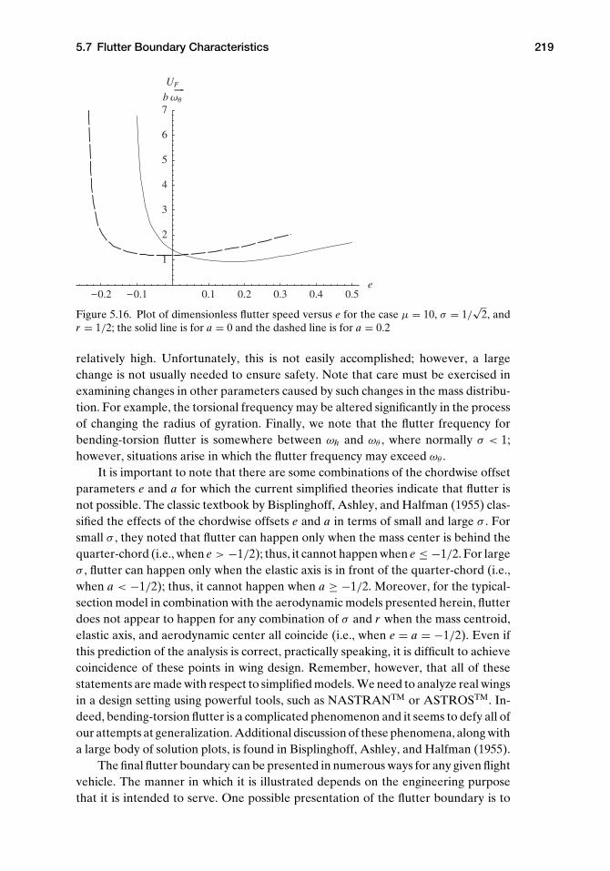
5.7 Flutter Boundary Characteristics 219
0.2 0.1 0.1 0.2 0.3 0.4 0.5e
1
2
3
4
5
6
7
UF
b
Figure 5.16. Plot of dimensionless flutter speed versus e for the case μ = 10, σ = 1/√
2, andr = 1/2; the solid line is for a = 0 and the dashed line is for a = 0.2
relatively high. Unfortunately, this is not easily accomplished; however, a largechange is not usually needed to ensure safety. Note that care must be exercised inexamining changes in other parameters caused by such changes in the mass distribu-tion. For example, the torsional frequency may be altered significantly in the processof changing the radius of gyration. Finally, we note that the flutter frequency forbending-torsion flutter is somewhere between ωh and ωθ , where normally σ < 1;however, situations arise in which the flutter frequency may exceed ωθ .
It is important to note that there are some combinations of the chordwise offsetparameters e and a for which the current simplified theories indicate that flutter isnot possible. The classic textbook by Bisplinghoff, Ashley, and Halfman (1955) clas-sified the effects of the chordwise offsets e and a in terms of small and large σ . Forsmall σ , they noted that flutter can happen only when the mass center is behind thequarter-chord (i.e., when e > −1/2); thus, it cannot happen when e ≤ −1/2. For largeσ , flutter can happen only when the elastic axis is in front of the quarter-chord (i.e.,when a < −1/2); thus, it cannot happen when a ≥ −1/2. Moreover, for the typical-section model in combination with the aerodynamic models presented herein, flutterdoes not appear to happen for any combination of σ and r when the mass centroid,elastic axis, and aerodynamic center all coincide (i.e., when e = a = −1/2). Even ifthis prediction of the analysis is correct, practically speaking, it is difficult to achievecoincidence of these points in wing design. Remember, however, that all of thesestatements are made with respect to simplified models. We need to analyze real wingsin a design setting using powerful tools, such as NASTRANTM or ASTROSTM. In-deed, bending-torsion flutter is a complicated phenomenon and it seems to defy all ofour attempts at generalization. Additional discussion of these phenomena, along witha large body of solution plots, is found in Bisplinghoff, Ashley, and Halfman (1955).
The final flutter boundary can be presented in numerous ways for any given flightvehicle. The manner in which it is illustrated depends on the engineering purposethat it is intended to serve. One possible presentation of the flutter boundary is to
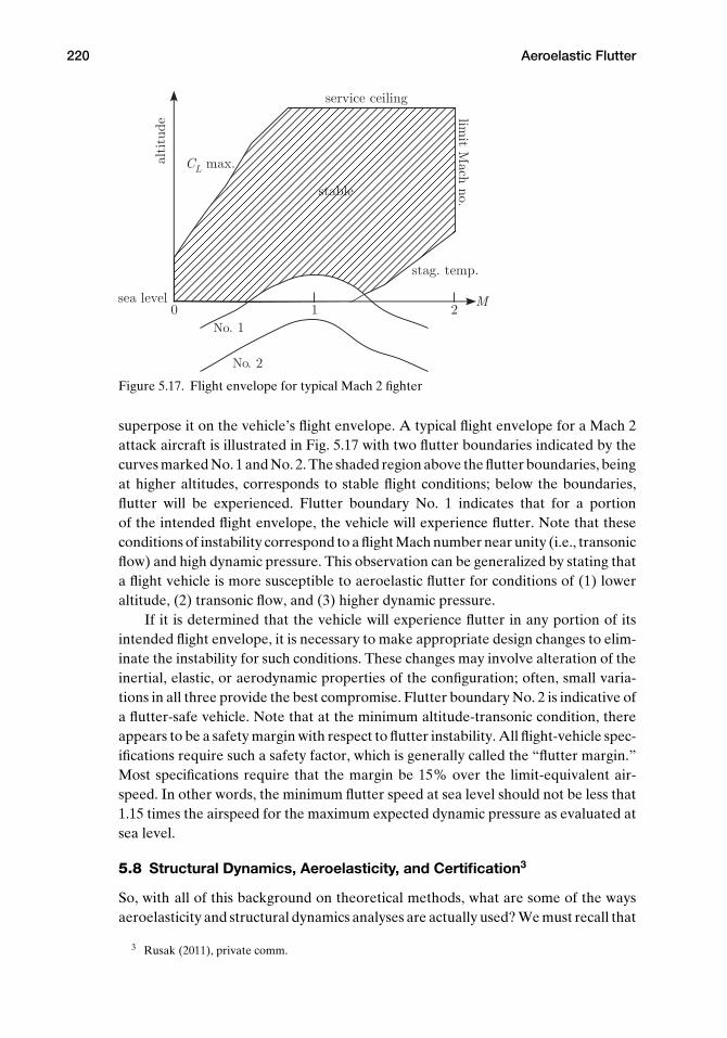
220 Aeroelastic Flutter
No
No
Figure 5.17. Flight envelope for typical Mach 2 fighter
superpose it on the vehicle’s flight envelope. A typical flight envelope for a Mach 2attack aircraft is illustrated in Fig. 5.17 with two flutter boundaries indicated by thecurves marked No. 1 and No. 2. The shaded region above the flutter boundaries, beingat higher altitudes, corresponds to stable flight conditions; below the boundaries,flutter will be experienced. Flutter boundary No. 1 indicates that for a portionof the intended flight envelope, the vehicle will experience flutter. Note that theseconditions of instability correspond to a flight Mach number near unity (i.e., transonicflow) and high dynamic pressure. This observation can be generalized by stating thata flight vehicle is more susceptible to aeroelastic flutter for conditions of (1) loweraltitude, (2) transonic flow, and (3) higher dynamic pressure.
If it is determined that the vehicle will experience flutter in any portion of itsintended flight envelope, it is necessary to make appropriate design changes to elim-inate the instability for such conditions. These changes may involve alteration of theinertial, elastic, or aerodynamic properties of the configuration; often, small varia-tions in all three provide the best compromise. Flutter boundary No. 2 is indicative ofa flutter-safe vehicle. Note that at the minimum altitude-transonic condition, thereappears to be a safety margin with respect to flutter instability. All flight-vehicle spec-ifications require such a safety factor, which is generally called the “flutter margin.”Most specifications require that the margin be 15% over the limit-equivalent air-speed. In other words, the minimum flutter speed at sea level should not be less that1.15 times the airspeed for the maximum expected dynamic pressure as evaluated atsea level.
5.8 Structural Dynamics, Aeroelasticity, and Certification3
So, with all of this background on theoretical methods, what are some of the waysaeroelasticity and structural dynamics analyses are actually used? We must recall that
3 Rusak (2011), private comm.

5.8 Structural Dynamics, Aeroelasticity, and Certification 221
for every aircraft, there may be dozens to several hundred combinations of fuel andpayloads that must be verified as stable within the aircraft’s flight envelope beforeclearance for flight is given. The use of computational results is crucial becausewe cannot possibly test every combination of fuel and hardware mounted on thefuselage and wings (e.g., stores, armaments, fuel tanks). Computational results thenbecome our main work tool for every go/no-go decision made in flight-testing andultimate airplane certification for flight.
To proceed with this monumental set of tasks, we first need to identify the mostcritical combinations (i.e., those with the lowest flutter speeds). If possible, theseshould be compared with previous experience in terms of computation and flight-testing. Once the most critical configurations are identified, we set them aside forspecial wind-tunnel and flight tests. In particular, we need to ascertain the fluttermode’s shape, frequency ωF , speed UF , and severity g′ = dg/dU, all evaluated atthe flutter speed (i.e., where g vanishes). Identification of all four items allows us todistinguish between various cases with comparable flutter speeds and, together withprevious experience, to decide about further needed ground and flight tests to verifycomputations and flight clearance.
5.8.1 Ground-Vibration Tests
The purpose of structural dynamics experiments on the ground is to validate the fre-quencies and mode shapes of a clean airplane or important airplane configurations.To accomplish this, the airplane is equipped with strain gages and accelerometersat the roots and tips of the wings, of the horizontal and vertical tails, and of the air-plane nose. The airplane is placed on soft supports to mimic the airplanes free-freestructural dynamics. Vertical actuators (i.e., shakers) are used at the tips of the wingand horizontal tail; both vertical and side shakers may be used at the tips of the noseand vertical tail. There is a variety of signal analysis methods to identify natural fre-quencies, mode shapes, and structural damping from the measurements. Generally,the actuators have a bandwidth up to 30 Hz, and a sweep of actuation frequencies isfirst conducted from 0.1 to 30 Hz to identify the symmetric and antisymmetric modesin this range. Classical techniques, such as Fast Fourier Transformation (FFT) andPower Spectral Density (PSD), are used for spectral analysis of unsteady elasticdeformation signals to identify the natural frequencies. At this point, we must con-tinue to study details of the dynamic response at the natural bending and torsionalfrequencies of interest for flutter or other aeroelastic phenomena. For each mode,this entails the following:
1. Induce oscillatory motion of the mode at a certain natural frequency, measurethe response, and perform an FFT analysis to identify the resonance frequencyand structural damping of that mode.
2. Induce a step-function command from oscillatory motion to zero, measure thedecay rate, and infer the structural damping of that mode.
3. Induce an impulsive function, measure the decay rate, and infer structural damp-ing of the mode.

222 Aeroelastic Flutter
Now we are ready to compare experimentally measured frequencies and modeshapes with detailed finite-element predictions. Using well-established techniques,we tune our finite element model to yield frequencies and mode shapes that fit theground-vibration test data.
5.8.2 Wind Tunnel Flutter Experiments
The design of wind tunnel models that accurately represent the flutter situations ofa real airplane is a complex task—quite possibly an art! The main challenge is tocompose a small-scale version of the aircraft with tuned structural dynamics and asufficiently detailed geometry that correctly reflects the aircraft’s static and unsteadyaerodynamic behavior. For these tests, the model is supported by soft cables andequipped with strain gages and accelerometers at the roots and tips of wings, at thetips of horizontal and vertical tails, and on the nose. Flow turbulence is used to excitethe model aeroelastic modes. FFT and PSD analysis of the various measured modeldeformations are used to estimate the flutter speed, frequency and severity.
The wind tunnel tests provide essential insight into the possible modes of flutterof an airplane. The tests help verify computed results as well as identify unknownaeroelastic phenomena related to the airplane configuration. However, it should berecognized that unsteady flow phenomena are strongly governed by scale, so thatreduced frequency, flow Reynolds number, separation between vortices, and interac-tions between shockwaves and boundary layers may not be correctly represented bysmall-scale models. In such experiments, results may lead to an inaccurate predictionof flutter occurrence in the full-scale airplane. In addition, testing of small-scale mod-els in the wind tunnel provides benchmark cases for improving the computationalmodels and tuning the unsteady aerodynamics analysis codes.
5.8.3 Ground Roll (Taxi) and Flight Tests
A special experimental aircraft is equipped with the capability of making realtimemeasurements of the amount of fuel, airspeed, Mach number, altitude, load factors,and control surface deflections. The aircraft is also instrumented as in the ground-vibration tests with strain gages and accelerometers. Special actuators are included tooperate the ailerons and elevators over a range of frequencies. A sweep of actuationfrequencies is first conducted to identify important modes. In addition, at certainfrequencies, responses to step and impulse commands are measured.
Ground Roll (Taxi) Measurements. Aircraft ground roll (taxi) provides the firstinsight into an airplane’s aeroelastic response. The relatively rough runway excitesthe airplane’s structural modes. In addition, here we conduct a sweep of frequenciesand FFT-PSD analyses of measurements and determine whether results match withanalysis predictions of aeroelastic behavior at near zero speeds. If they do not, wemust stop the test to correct and/or adjust the computational model until agreementis found, and then flutter predictions are reevaluated. Only when results do agree,may we then proceed to take off.

5.8 Structural Dynamics, Aeroelasticity, and Certification 223
Flight Tests. In this step, we take off and fly at the lowest speed at low altitude andin level flight. We measure the airplane’s response to air turbulence and conductFFT and PSD analyses. We determine whether these results match our analyticalpredictions for the tested speed. If they do not, we must again stop the test to correctand/or adjust the computational model until we find agreement. When they do agree,we then may proceed to activate the actuators for an impulse command. Next, wedetermine whether there is sufficient damping. If there is, we conduct a sweep offrequencies and conduct FFT and PSD analyses of frequencies and damping. Ifthese results match the analysis, then we may (cautiously!) activate actuators at thecalculated flutter frequency and conduct FFT and PSD analyses of the response.When the damping measurements match theoretical predictions, then we activateactuators for a step command. Next, we determine whether the response matchesthe analysis. When it does, we then collect and store data in the form of U-g-g′
diagrams. Only if and when there is reasonable agreement with analyses we proceedcautiously to perform maneuvers at various load factors at the same speed andaltitude. During each maneuver, we activate the actuators for an impulse commandto see whether there is sufficient damping. If there is, we move on to increase the loadfactor until the complete set of specified load factors within the flight envelope istested.
If our computed predictions are in agreement with the results obtained at anystage, only then is it safe to go to a higher speed (e.g., 25 knots faster) at the samealtitude. At this point we repeat all of the steps, collecting and storing data in the formof U-g-g′ diagrams. We systematically and cautiously increase the speed up to itsmaximum, checking at every increment to ensure that our analysis is valid. Similarly,we systematically increase altitude to its maximum and repeat the regimen. We stop(i.e., reduce speed to the previous safe speed) immediately whenever any one of thefollowing happens:
1. A modal damping coefficient g decreases below the level of damping requiredby regulations (5% in a civil aircraft).
2. Oscillations in at least one measurement diverge and grow beyond preapprovedlimits.
3. The dominant frequency deviates from its predicted value.
Thus, it is observed that the analysis of airplane flutter is strongly based ontheoretical studies. The theory is the work tool for analysis and decisions aboutcritical configurations and flight conditions. Ground vibration experiments are usedto tune the structural dynamics analysis to yield accurate structural modes, and windtunnel experiments to tune the unsteady aerodynamics code. Flutter flight tests areextremely dangerous. Real-time measurements and various actuation techniquesare used to estimate the damping of the airplane at various flight altitudes, speeds,and load factors and move from one point to another with much caution. Analysis,ground experiments and flight tests always go together to provide full clearance forflight without flutter problems.

224 Aeroelastic Flutter
5.8.4 Flutter Flight Tests
In this step, we take off and fly at the lowest speed at low altitude and in level flight.We then measure the response due to air turbulence and conduct FFT and PSDanalyses. We determine whether these results match our analytical predictions. Ifthey do not, we must again correct and/or adjust the model until we obtain agree-ment. When they eventually agree, we then may proceed to activate the actuatorsfor an impulse command. Next, we determine whether there is sufficient damping.If there is, we conduct a sweep of frequencies and conduct FFT and PSD analysesof frequencies and damping. If these results match the analyses, then we may (cau-tiously!) activate actuators at the calculated flutter frequency and conduct FFT andPSD analyses of the response. When the damping measurements match the theo-retical predictions, we activate actuators for a step command. Next, we determinewhether the response matches the analyses. When it does, we collect and store datain the form of U − g − g′ diagrams. Only if and when there is reasonable agreementwith analyses may we proceed to perform a 2g maneuver at the same speed andaltitude. At this level of gs, we activate the actuators for an impulse command to seewhether there is sufficient damping. If there is, we move on to 3g, then 4g, and soon, all at the same airspeed and altitude, until we have tested the complete set ofspecified load factors within the flight envelope.
If our model is still in agreement with the results obtained at any stage, only thenis it safe to go to a higher speed (e.g., 25 knots faster) at the same altitude. At thispoint, we repeat all of the steps and collect data in the form of U − g − g′ diagrams.We systematically and cautiously increase the speed up to its maximum, checkingat every increment to ensure that our analysis is valid. Similarly, we systematicallyincrease altitude to its maximum and repeat the regimen. We stop (i.e., reducespeed to the previous safe speed) immediately whenever any one of the followinghappens:
1. There is even the slightest indication that the damping coefficient g decreasesbelow 2% (5% in a civil aircraft).
2. Oscillations in at least one of the measurements diverge and tend to grow beyondpreapproved limits.
3. The dominant frequency deviates from the predicted mode frequency.
Thus, it is observed that the analysis of flutter is strongly based on theoreticalstudies. The theory is the work tool for analysis and decisions about critical config-urations and flight conditions. Ground-vibration experiments are used to tune theanalysis to yield accurate structural-dynamics modes and wind-tunnel experimentsto tune the unsteady-aerodynamics code.
Flutter flight tests are extremely dangerous. Real-time measurements and vari-ous actuation techniques are used to estimate the damping of the airplane at variousflight altitudes, speeds, and load factors, moving from one point to another withcaution. Analysis, ground experiments, and flight tests always go together to providefull clearance for flight without any flutter problems.

Problems 1–2 225
5.9 Epilogue
In this chapter, we consider the general problem of lifting-surface flutter. Severaltypes of flutter analysis were presented, including the p method, classical flutteranalysis, k method, and p-k method. The application of classical flutter analysis todiscrete one- and two-degree-of-freedom wind-tunnel models was presented. Stu-dents were exposed to Theodorsen’s unsteady thin-airfoil theory along with the moremodern finite-state thin-airfoil theory of Peters et al. Application of the assumed-modes method to construct a flutter analysis of a flexible wing was demonstrated aswell. The important parameters of the flutter problem were discussed, along withcurrent design practice, flight testing, and certification. With a good understandingof the material presented herein, students should be sufficiently equipped to applythese fundamentals to the design of flight vehicles.
Moreover, with appropriate graduate-level studies well beyond the scope ofmaterial presented herein, students will be able to conduct research in the excitingfield of aeroelasticity. Current research topics are quite diverse. With the increasedsophistication of controls technology, it has become more common to attack flutterproblems by active control of flaps or other flight-control surfaces. These so-calledflutter-suppression systems provide alternatives to costly design changes. One typeof system for which flutter-suppression systems are an excellent choice is a militaryaircraft that must carry weapons as stores. These aircraft must be free of flutterwithin their flight envelope for different configurations, sometimes many differentconfigurations. At times, avoidance of flutter by design changes is simply beyond thecapability of designers for such complex systems. There is also a body of researchto determine in flight when a flutter boundary is being approached. This could be ofgreat value for situations in which damage had altered the properties of the aircraftstructure—perhaps unknown to the pilot—thus shifting the flutter (or divergence)boundary and making the aircraft unsafe to operate within its original flight envelope.Other current problems of interest to aeroelasticians include improved analysismethodology for prediction of flutter, gust response, and limit-cycle oscillations;design of control systems to improve gust response and limit-cycle oscillations; andincorporation of aeroelastic analyses at an earlier stage of aircraft design.
Problems
1. Compute the flutter speed for the incompressible, one-degree-of-freedom flutterproblem with
mθ = i − 2k
− 10i
IP = 50πρ∞b4 ωθ = 10 Hz b = 0.5 ft
Answer: UF = 405.6 ft/sec
2. According to Theodorsen’s theory, the circulatory lift is proportional to a quan-tity that for simple harmonic motion can be shown to be equal to the effective

226 Aeroelastic Flutter
angle of attack given by
α = C(k)[θ + h
U+ b
U
(12
− a)
θ
]
For a = −1/2 and simple harmonic motion such that θ = 1 and h =bz [cos(φ) + i sin(φ)], find the amplitude and phase of α relative to θ and plot α
as a function of time for five periods for the following four cases:(a) z = 0.1; φ = 0◦; k = 0.01(b) z = 0.1; φ = 0◦; k = 1.0(c) z = 0.1; φ = 90◦; k = 1.0(d) z = 0.5; φ = 90◦; k = 1.0Comment on the behavior of α for increasing k, changing the phase angle from 0to 90 degrees, and increasing the plunge magnitude. Approximate Theodorsen’sfunction as
C(k) = 0.01365 + 0.2808ik − k2
2
0.01365 + 0.3455ik − k2
Answer: (a) amplitude: 0.9931; phase lead: 2.01◦
Answer: (b) amplitude: 0.7988; phase lag: 37.0◦
Answer: (c) amplitude: 0.7229; phase lag: 37.3◦
Answer: (d) amplitude: 0.6008; phase lag: 52.7◦
3. Show that the coefficients used in a classical flutter analysis, if based onTheodorsen’s theory, are
�h = 1 − 2iC(k)k
�θ = − a − ik
− 2C(k)k2
− 2i( 1
2 − a)
C(k)
k
mh = −a + 2i( 1
2 + a)
C(k)
k
mθ = 18
+ a2 − i( 1
2 − a)
k+ 2
( 12 + a
)C(k)
k2+ 2i
( 14 − a2
)C(k)
k
4. Consider a two-dimensional rigid wing in incompressible flow with freestreamspeed U and pivoted about the leading edge. The pitch motion is spring-restrained with spring constant kθ = IPω2
θ . Use the exact C(k) and(a) determine the flutter speed and flutter frequency for IP = 2,500πρ∞b4
(b) determine the minimum possible flutter speed and flutter frequencyAnswer: (a) UF = 28.2279 bωθ and ωF = 1.13879 ωθ ; (b) UF = 24.7877 bωθ and
ωF = ωθ
5. Consider an incompressible, two-degree-of-freedom flutter problem in whicha = −1/5, e = −1/10, μ = 20, r2 = 6/25, and σ = 2/5. Compute the flutter speed

Problems 5–14 227
and the flutter frequency using the classical flutter approach. For the aerody-namic coefficients, use those of Theodorsen’s theory with C(k) approximated asin Problem 2.Answer: UF = 2.170 bωθ and ωF = 0.6443 ωθ
6. Consider an incompressible, two-degree-of-freedom flutter problem in whicha = −1/5, μ = 3, and r = 1/2. Compute the flutter speed and flutter frequencyfor two cases xθ = e − a = 1/5 and xθ = e − a = 1/10, and let σ = 0.2, 0.4, 0.6,0.8, and 1.0. Use the classical flutter approach and, for the aerodynamic coeffi-cients, use those of Theodorsen’s theory with C(k) approximated as in Problem2. Compare with the results in Fig. 5.15.
7. Set up the complete set of equations for flutter analysis by the p method usingthe unsteady-aerodynamic theory of Peters et al. (1995), nondimensionalizingEqs. (5.106), and redefining λi as bωθλi .
8. Write a computer program using MATLABTM or MathematicaTM to set up thesolution of the equations derived in Problem 7.
9. Using the computer program written in Problem 8, solve for the dimensionlessflutter speed and flutter frequency for an incompressible, two-degree-of-freedomflutter problem in which a = −1/3, e = −1/10, μ = 50, r = 2/5, and σ = 2/5.Answer: UF = 2.807 bωθ and ωF = 0.5952 ωθ
10. Write a computer program using MATLABTM or MathematicaTM to set up thesolution of a two-degree-of-freedom flutter problem using the k method.
11. Use the computer program written in Problem 10 to solve a flutter problemin which a = −1/5, e = −1/10, μ = 20, r2 = 6/25, and σ = 2/5. Plot the valuesof ω1,2/ωθ and g versus U/(bωθ ) and compare your results with the quanti-ties plotted in Figs. 5.12 and 5.13. Noting how the quantities plotted in thesetwo sets of figures are different, comment on the similarities and differencesobserved in these plots and why those differences are there. Finally, explainwhy your predicted flutter speed is the same as that determined by the classicalmethod.Answer: See Figs. 5.18 and 5.19.
12. Show that the flutter determinant for the p-k method applied to the typicalsection using Theodorsen aerodynamics can be expressed as
∣∣∣∣∣∣p2 + σ 2
V2 − k2
μ+ 2ikC(k)
μ
p2μxθ +k(i+ak)+[2+ik(1−2a)]C(k)μ
p2μxθ+ak2−ik(1+2a)C(k)μ
8μr2(
p2+ 1V2
)+4i(1+2a)[2i−k(1−2a)]C(k)−k[k−4i+8a(i+ak)]
8μ
∣∣∣∣∣∣13. Write a computer program using MATLABTM or MathematicaTM to set up the
solution of a two-degree-of-freedom flutter problem using the p-k method andTheodorsen aerodynamics.
14. Use the computer program written in Problem 13 to solve a flutter problem inwhich a = −1/5, e = −1/10, μ = 20, r2 = 6/25, and σ = 2/5. Plot the values of

228 Aeroelastic Flutter
0.0 0.5 1.0 1.5 2.0 2.5
U
bωθ
0.2
0.4
0.6
0.8
1.0
ωθ
Figure 5.18. Plot of ω1,2/ωθ versus U/(bωθ ) using the k method and Theodorsen aerodynamicswith a = −1/5, e = −1/10, μ = 20, r 2 = 6/25, and σ = 2/5
the estimates of �1,2/ωθ and �1,2/ωθ versus U/(bωθ ) and compare your resultswith the quantities plotted in Figs. 5.12 and 5.13. Explain why the estimateddamping from the p-k method sometimes differs from that of the p method.Answer: See Figs. 5.20 and 5.21.
0.5 1.0 1.5 2.0 2.5
U
bωθ
0.8
0.6
0.4
0.2
0.2
g
Figure 5.19. Plot of g versus U/(bωθ ) using the k method and Theodorsen aerodynamics witha = −1/5, e = −1/10, μ = 20, r 2 = 6/25, and σ = 2/5

Problems 15–16 229
0.0 0.5 1.0 1.5 2.0 2.5
U
b ωθ
0.2
0.4
0.6
0.8
1.0
ωθ
Figure 5.20. Plot of estimated value of �1,2/ωθ versus U/(bωθ ) using the p-k method withTheodorsen aerodynamics (dashed lines) and the p method with the aerodynamics of Peterset al. (solid lines) for a = −1/5, e = −1/10, μ = 20, r 2 = 6/25, and σ = 2/5
15. Write a computer program using MATLABTM or MathematicaTM to set up thesolution of a two-degree-of-freedom flutter problem using the p-k method andthe aerodynamics of Peters et al.
16. Using the computer programs of Problems 13 and 15, show that the p-kmethod yields the same results regardless of whether Theodorsen’s theory or the
0.5 1.0 1.5 2.0 2.5
U
b ωθ
0.5
0.4
0.3
0.2
0.1
0.1
ωθ
Figure 5.21. Plot of estimated value of �1,2/ωθ versus U/(bωθ ) using the p-k method withTheodorsen aerodynamics (dashed lines) and the p method with the aerodynamics of Peterset al. (solid lines) for a = −1/5, e = −1/10, μ = 20, r 2 = 6/25, and σ = 2/5

230 Aeroelastic Flutter
aerodynamic theory of Peters et al. is used, assuming a sufficiently large numberof inflow states is used in the latter. You may do this for the case a = −1/5,e = −1/10, μ = 20, r2 = 6/25, and σ = 2/5. What does this imply about the twotheories?
17. Write a computer program to solve for the flutter speed of the problem set upin Section 5.6. Exercise the code for the parameters of Problem 16 and examinethe sensitivity of the results to the number of modes assumed.
18. Repeat the derivation in Section 5.6 but use the finite element method.19. Write a computer program based on Problem 18 and compare the answers
obtained with those of Problem 17 with one bending mode and one torsionmode. Determine the sensitivity of the predicted flutter speed and frequencyto the number of elements and the number of elements required for resultsconverged to four significant figures.
20. Repeat Problem 18 but use the aerodynamic theory of Peters et al. with a set ofstates located at points x = ri� with r1 < r2 < . . . < rm, where m is the numberof sets of aerodynamic states.
21. Write a computer program based on Problem 20. Determine the sensitivity ofthe results to the number and values of parameters ri , in which the latter areequally spaced along the span.
22. Comparing Eqs. (5.11) and (5.71), find an expression for [A(p)] in terms ofmatrices [a], [b], [c], [d], [A], and [E] for the special case when the only de-grees of freedom in the column matrix ξ are h/b and θ , and the unsteady-aerodynamic theory is based on the theory of Peters et al. with six states. As-suming simple harmonic motion, extract an approximation for C(k) from theseequations. Compare the real and imaginary parts of C(k) with those from theapproximation.

APPENDIX A
Lagrange’s Equations
A.1 Introduction
When we wish to use Newton’s laws to write the equations of motion of a particle ora system of particles, we must be careful to include all the forces of the system. TheLagrangean form of the equations of motion that we derive herein has the advantagethat we can ignore all forces that do no work (e.g., forces at frictionless pins, forcesat a point of rolling contact, forces at frictionless guides, and forces in inextensibleconnections). In the case of conservative systems (i.e., systems for which the totalenergy remains constant), the Lagrangean method gives us an automatic procedurefor obtaining the equations of motion provided only that we can write the kineticand potential energies of the system.
A.2 Degrees of Freedom
Before proceeding to develop the Lagrange equations, we must characterize ourdynamical systems in a systematic way. The most important property of this sort forour present purpose is the number of independent coordinates that we must knowto completely specify the position or configuration of our system. We say that asystem has n degrees of freedom if exactly n coordinates serve to completely defineits configuration.
EXAMPLE 1 A free particle in space has three degrees of freedom because wemust know three coordinates—x, y, z, for example – to locate it.
EXAMPLE 2 A wheel that rolls without slipping on a straight track has one degreeof freedom because either the distance from some base point or the total angleof rotation will enable us to locate it completely.
A.3 Generalized Coordinates
We usually think of coordinates as lengths or angles. However, any set of parametersthat enables us to uniquely specify the configuration of the system can serve as
231

232 Appendix A: Lagrange’s Equations
coordinates. When we generalize the meaning of the term in this manner, we callthese new quantities “generalized coordinates.”
EXAMPLE 3 Consider a bar rotating in a plane about a point O. The angle ofrotation with respect to some base line is suggested as an obvious coordinatefor specifying the position of the bar. However, the area swept over by thebar would do equally well and therefore could be used as a generalized co-ordinate.
If a system has n degrees of freedom, then n generalized coordinates are neces-sary and sufficient to determine the configuration.
A.4 Lagrange’s Equations
In deriving these equations, we consider systems having two degrees of freedom andhence are completely defined by two generalized coordinates q1 and q2. However,the results are easily extended to systems with any number of degrees of freedom.
Suppose our system consists of n particles. For each particle, we can write byNewton’s second law
Mi xi = Xi
Mi yi = Yi
Mi zi = Zi
(A.1)
where xi , yi , and zi are the rectangular Cartesian coordinates of the ith particle; Mi
is the mass; and Xi , Yi , and Zi are the resultants of all forces acting on it in the x, y,and z directions, respectively.
If we multiply both sides of Eqs. (A.1) by δxi , δyi , and δzi , respectively, and addthe equations, we have
Mi (xiδxi + yiδyi + ziδzi ) = Xiδxi + Yiδyi + Ziδzi (A.2)
The right-hand side of this equation represents the work done by all of the forcesacting on the ith particle during the virtual displacements δxi , δyi , and δzi . Hence,forces that do no work do not contribute to the right-hand side of Eq. (A.2) and maybe omitted from the equation. To obtain the corresponding equation for the entiresystem, we sum both sides of Eq. (A.2) for all particles. Thus
n∑i=1
Mi (xiδxi + yiδyi + ziδzi ) =n∑
i=1
(Xiδxi + Yiδyi + Ziδzi ) (A.3)
Now, because our system is completely located in space if we know the twogeneralized coordinates q1 and q2, we must be able to write xi , yi , and zi as well as

Appendix A: Lagrange’s Equations 233
their increments δxi , δyi , and δzi as functions of q1 and q2. Hence
xi = xi (q1, q2)
yi = yi (q1, q2)
zi = zi (q1, q2)
(A.4)
Differentiating Eq. (A.4) with respect to time gives
xi = ∂xi
∂q1q1 + ∂xi
∂q2q2
yi = ∂yi
∂q1q1 + ∂yi
∂q2q2
zi = ∂zi
∂q1q1 + ∂zi
∂q2q2
(A.5)
Similarly
δxi = ∂xi
∂q1δq1 + ∂xi
∂q2δq2
δyi = ∂yi
∂q1δq1 + ∂yi
∂q2δq2
δzi = ∂zi
∂q1δq1 + ∂zi
∂q2δq2
(A.6)
If we substitute these into Eq. (A.3) and rearrange the terms, we obtain
n∑i=1
[Mi
(xi
∂xi
∂q1+ yi
∂yi
∂q1+ zi
∂zi
∂q1
)δq1
+ Mi
(xi
∂xi
∂q2+ yi
∂yi
∂q2+ zi
∂zi
∂q2
)δq2
]
=n∑
i=1
[(Xi
∂xi
∂q1+ Yi
∂yi
∂q1+ Zi
∂zi
∂q1
)δq1
+(
Xi∂xi
∂q2+ Yi
∂yi
∂q2+ Zi
∂zi
∂q2
)δq2
]
(A.7)
From Eq. (A.5), we conclude that because xi , yi , and zi are functions of q1 and q2
but not of q1 and q2, then
∂ xi
∂q1= ∂xi
∂q1
∂ xi
∂q2= ∂xi
∂q2
∂ yi
∂q1= ∂yi
∂q1
∂ yi
∂q2= ∂yi
∂q2
∂ zi
∂q1= ∂zi
∂q1
∂ zi
∂q2= ∂zi
∂q2
(A.8)

234 Appendix A: Lagrange’s Equations
We substitute these relationships into the left-hand side of Eq. (A.7) to obtain
n∑i=1
[Mi
(xi
∂ xi
∂q1+ yi
∂ yi
∂q1+ zi
∂ zi
∂q1
)δq1
+ Mi
(xi
∂ xi
∂q2+ yi
∂ yi
∂q2+ zi
∂ zi
∂q2
)δq2
]
=n∑
i=1
[(Xi
∂xi
∂q1+ Yi
∂yi
∂q1+ Zi
∂zi
∂q1
)δq1
+(
Xi∂xi
∂q2+ Yi
∂yi
∂q2+ Zi
∂zi
∂q2
)δq2
]
(A.9)
Now, let us shift our attack on the problem and consider the kinetic energy ofthe system. This is
K = 12
n∑i=1
Mi(x2
i + y2i + z2
i
)(A.10)
Now calculate ∂K∂q1
and ∂K∂q2
to obtain
∂K∂q1
=n∑
i=1
Mi
(xi
∂ xi
∂q1+ yi
∂ yi
∂q1+ zi
∂ zi
∂q1
)(A.11)
∂K∂q1
=n∑
i=1
Mi
(xi
∂ xi
∂q1+ yi
∂ yi
∂q1+ zi
∂ zi
∂q1
)(A.12)
We next calculate the time derivative of ∂xi∂q1
, for which the chain rule gives
ddt
(∂xi
∂q1
)= ∂2xi
∂q21
q1 + ∂2xi
∂q1∂q2q2
= ∂
∂q1
(∂xi
∂q1q1 + ∂xi
∂q2q2
)
= ∂
∂q1(xi ) = ∂ xi
∂q1
(A.13)
Because from Eq. (A.8) we have
∂ xi
∂q1= ∂xi
∂q1(A.14)
we conclude from Eq. (A.13) that
ddt
(∂xi
∂q1
)= ∂ xi
∂q1(A.15)

Appendix A: Lagrange’s Equations 235
The following relationships can be proven in a similar manner:
ddt
(∂yi
∂q1
)= ∂ yi
∂q1
ddt
(∂zi
∂q1
)= ∂ zi
∂q1
(A.16)
Now let us use Eqs. (A.11), (A.12), (A.15), and (A.16) to calculate the function
ddt
(∂K∂q1
)− ∂K
∂q1(A.17)
for which the result is
ddt
(∂K∂q1
)− ∂K
∂q1=
n∑i=1
Mi
(xi
∂ xi
∂q1+ yi
∂ yi
∂q1+ zi
∂ zi
∂q1
)
+n∑
i=1
Mi
[xi
ddt
(∂ xi
∂q1
)+ yi
ddt
(∂ yi
∂q1
)+ zi
ddt
(∂ zi
∂q1
)]
−n∑
i=1
Mi
(xi
∂ xi
∂q1+ yi
∂ yi
∂q1+ zi
∂ zi
∂q1
)(A.18)
From Eqs. (A.15) and (A.16), the second and third terms on the right-hand side ofEq. (A.18) are equal and thus cancel, leaving
ddt
(∂K∂q1
)− ∂K
∂q1=
n∑i=1
Mi
(xi
∂ xi
∂q1+ yi
∂ yi
∂q1+ zi
∂ zi
∂q1
)(A.19)
A similar relationship holds for partial derivatives of K with respect to q2 and q2.Hence, Eq. (A.9) can be written[
ddt
(∂K∂q1
)− ∂K
∂q1
]δq1 +
[ddt
(∂K∂q2
)− ∂K
∂q2
]δq2
=n∑
i=1
(Xi
∂xi
∂q1+ Yi
∂yi
∂q1+ Zi
∂zi
∂q1
)δq1
+n∑
i=1
(Xi
∂xi
∂q2+ Yi
∂yi
∂q2+ Zi
∂zi
∂q2
)δq2
(A.20)
Because q1 and q2 are independent coordinates, they can be varied arbitrarily. Hence,we can conclude that
ddt
(∂K∂q1
)− ∂K
∂q1=
n∑i=1
(Xi
∂xi
∂q1+ Yi
∂yi
∂q1+ Zi
∂zi
∂q1
)
ddt
(∂K∂q2
)− ∂K
∂q2=
n∑i=1
(Xi
∂xi
∂q2+ Yi
∂yi
∂q2+ Zi
∂zi
∂q2
) (A.21)

236 Appendix A: Lagrange’s Equations
The right-hand side of Eq. (A.20) is the work done by all of the forces on thesystem when the coordinates of the ith particle undergo the small displacement δxi ,δyi , and δzi due to changes δq1 and δq2 in the generalized coordinates q1 and q2. Thecoefficients of δq1 and δq2 are known as the generalized forces Q1 and Q2 becausethey are the quantities by which the variations of the generalized coordinates mustbe multiplied to calculate the virtual work done by all the forces acting on the system.Hence
Q1 =n∑
i=1
(Xi
∂xi
∂q1+ Yi
∂yi
∂q1+ Zi
∂zi
∂q1
)
Q2 =n∑
i=1
(Xi
∂xi
∂q2+ Yi
∂yi
∂q2+ Zi
∂zi
∂q2
) (A.22)
and Eqs. (A.21) can be written
ddt
(∂K∂q1
)− ∂K
∂q1= Q1
ddt
(∂K∂q2
)− ∂K
∂q2= Q2
(A.23)
This is one form of Lagrange’s equations of motion. They apply to any system that iscompletely described by two and only two generalized coordinates, whether or notthe system is conservative. It can be shown by slightly more extended calculationthat they apply to systems of any finite number of degrees of freedom.
A.5 Lagrange’s Equations for Conservative Systems
If a system is conservative, the work done by the forces can be calculated fromthe potential energy P. We define the change in potential energy during a smalldisplacement as the negative of the work done by the forces of the system duringthe displacement. Because Q1δq1 + Q2δq2 is the work done by the forces, we have
δP = −Q1δq1 − Q2δq2 (A.24)
We have emphasized that q1 and q2 are independent and, hence, can be variedarbitrarily. If δq2 = 0, we have δP = −Q1δq1 so that
Q1 = − ∂ P∂q1
(A.25)
Similarly, it can be seen that
Q2 = − ∂ P∂q2
(A.26)

Appendix A: Lagrange’s Equations 237
Figure A.1. Schematic for the mechanical systemof Example 5
Replacing Q1 and Q2 in Eqs. (A.23) by these expressions, we have
ddt
(∂K∂q1
)− ∂K
∂q1+ ∂ P
∂q1= 0
ddt
(∂K∂q2
)− ∂K
∂q2+ ∂ P
∂q2= 0
(A.27)
These are Lagrange’s equations of motion for a conservative system. As before, theyhold for systems of any finite number of degrees of freedom.
EXAMPLE 4 Find the equations of motion of a particle of weight W moving inspace under the force of gravity.Solution: We need three coordinates to describe the position of the particle andcan therefore take x, y, and z as the generalized coordinates. Taking x and y inthe horizontal plane and z vertically upward with the origin at the earth’s surfaceand taking the origin as the zero position for potential energy, we obtain
K = W2g
(x2 + y2 + z2) P = Wz
∂K∂ x
= Wg
x∂K∂ y
= Wg
y∂K∂ z
= Wg
z∂K∂x
= ∂K∂y
= ∂K∂z
= 0
ddt
(∂K∂ x
)= W
gx
ddt
(∂K∂ y
)= W
gy
ddt
(∂K∂ z
)= W
gz
∂ P∂x
= ∂ P∂y
= 0∂ P∂z
= W
(A.28)
Hence, Lagrange’s equation, Eq. (A.27), gives
Wg
x = 0Wg
y = 0Wg
z + W = 0 (A.29)
Of course, these equations are more easily obtainable by the direct applica-tion of Newton’s second law; this example merely illustrates the application ofLagrange’s equations for a familiar problem.
EXAMPLE 5 Find the equation of motion of the sprung weight W sliding on asmooth horizontal plane (Fig. A.1).

238 Appendix A: Lagrange’s Equations
Figure A.2. Schematic for the mechanical sys-tem of Example 6
Solution: We may take x as the generalized coordinate and measure it from theequilibrium position. Then
K = W2g
x2 P = k2
x2
∂K∂ x
= Wg
xddt
(∂K∂ x
)= W
gx
∂K∂x
= 0∂ P∂x
= kx
(A.30)
Lagrange’s equation, Eq. (A.27), gives
Wg
x + kx = 0 (A.31)
as the equation of motion.
EXAMPLE 6 Obtain the equations of motion for the system shown in Fig. A.2.The bar is weightless.Solution: The coordinates x1 and x2 can be taken as generalized coordinates.Take as the zero datum the configuration for which the bar is horizontal and thespring is unstretched. Then
K = W2g
x21 + W
2gx2
2 P = Wx1 − Wx2 + 12
k(x2 − x1)2
∂K∂ x1
= Wg
x1∂K∂ x2
= Wg
x2∂K∂x1
= ∂K∂x2
= 0
ddt
(∂K∂ x1
)= W
gx1
ddt
(∂K∂ x2
)= W
gx2
∂ P∂x1
= W − k(x2 − x1)∂ P∂x2
= −W + k(x2 − x1)
(A.32)
The Lagrange equations are
Wg
x1 + W − k(x2 − x1) = 0
Wg
x2 − W + k(x2 − x1) = 0
(A.33)
This is an example of a two-degree-of-freedom conservative system.

Appendix A: Lagrange’s Equations 239
A.6 Lagrange’s Equations for Nonconservative Systems
If the system is nonconservative, then, in general, there are some forces (i.e., conser-vative) that are derivable from a potential function, P(q1, q2, . . .) and some forces(i.e., nonconservative) that are not. Those forces for which a potential function doesnot exist must be introduced by first determining their virtual work. The coefficientof the virtual displacement δqi in the virtual-work expression is the generalized force,here denoted by Qi (i = 1, 2, . . .). In this instance, it is convenient to introduce whatis called the Lagrangean as
L = K − P (A.34)
and write the general form of Lagrange’s equations as
ddt
(∂L∂qi
)− ∂L
∂qi= Qi (i = 1, 2, . . . , n) (A.35)
EXAMPLE 7 Rework Example 5 with a dashpot of constant c connected in parallelwith the spring.Solution: The system with a dashpot is nonconservative. Hence, we use Lag-range’s equations in the form of Eq. (A.35). The kinetic and potential energiesare the same as in Example 5. To calculate the Q for the dashpot force, use thedefinition that Q is the coefficient by which the generalized coordinates mustbe multiplied to obtain the work done. In any small displacement δx, the workdone by the dashpot force −cx is −cx δx. Hence, −cx is the generalized forceassociated with the dashpot. The Lagrangean is
L = Wx2
2g− kx2
2(A.36)
and
Q = −cx (A.37)
Lagrange’s equation then becomes
Wg
x + kx = −cx (A.38)


References
Structural Dynamics
1. Bisplinghoff, R. L., H. Ashley, and R. L. Halfman, Aeroelasticity, Addison-Wesley Pub-lishing Co., Inc., 1955.
2. Chen, Y., Vibrations: Theoretical Methods, Addison-Wesley Publishing Co., Inc., 1966.3. Frazer, R. A. and Duncan, W. J., “The Flutter of Aeroplane Wings,” R&M 1155, Aero-
nautical Research Council, August 1928.4. Fry’ba, L., Vibration and Solids and Structures under Moving Loads, Noordhoff Interna-
tional Publishing, 1972.5. Hodges, D. H., Nonlinear Composite Beam Theory, AIAA, 2006.6. Hurty, W. C., and M. F. Rubenstein, Dynamics of Structures, Prentice-Hall, Inc., 1964.7. Kalnins, A., and C. L. Dym, Vibration: Beams, Plates and Shells, Dowden, Hutchinson
and Ross, Inc., 1976.8. Lamb, H., The Dynamical Theory of Sound, 2nd Edition 1925 (reprinted by Dover).9. Leipholz, H., Direct Variational Methods and Eigenvalue Problems in Engineering,
Noordhoff International Publishing, 1977.10. Lin, Y. K., Probabilistic Theory of Structural Dynamics, McGraw-Hill, Inc., 1967,
reprinted by Robert E. Krieger Publishing Co., 1976.11. Meirovitch, L., Computational Methods in Structural Dynamics, Sijthoff and Noordhoff,
1980.12. Meirovitch, L., Principles and Techniques of Vibrations, Prentice-Hall, Inc., 1997.13. Pestel, E. C., and F. A. Leckie, Matrix Methods in Elastomechanics, McGraw-Hill Book
Co., Inc., 1963.14. Rayleigh, J. W. S., The Theory of Sound, Vol. I, 1877, The MacMillan Co., 1945 (reprinted
by Dover).15. Reddy, J. N., An Introduction to the Finite Element Method, McGraw-Hill Book Co., Inc.,
1993.16. Roxbee Cox, H., and Pugsley, A. G., “Theory of Loss of Lateral Control Due to Wing
Twisting,” R&M 1506, Aeronautical Research Council, October 1932.17. Scanlan, R. H., and R. Rosenbaum, Introduction to the Study of Aircraft Vibration and
Flutter, The MacMillan Co., 1951 (reprinted by Dover).18. Simitses, G. J., and D. H. Hodges, Structural Stability, Vol. 3, Pt. 13. In: Encyclopedia of
Aerospace Engineering, Eds. R. Blockley and W. Shyy, John Wiley & Sons, 2010.19. Snowdon, J. C., Vibration and Shock in Damped Mechanical Systems, John Wiley and
Sons, 1968.20. Steidel, R. F., Jr., An Introduction to Mechanical Vibrations, 2nd ed., John Wiley and
Sons, 1979.21. Thomson, W. T., and M. D. Dahleh, Theory of Vibration with Applications, 5th ed.,
Prentice-Hall, Inc., 1998.22. Timoshenko, S., and D. H. Young, Vibration Problems in Engineering, 3rd ed., Van
Nostrand Reinhold Co., 1955.
241

242 References
23. Tse, F. S., I. E. Morse, and R. T. Hinkle, Mechanical Vibrations: Theory and Applications,2nd ed., Allyn and Bacon, Inc., 1978.
24. Zienkiewicz, O. C., and Taylor, R. L., The Finite Element Method for Solid and StructuralMechanics, Elsevier Butterworth-Heinemann, 2005.
Aeroelasticity
1. Abramson, H. N., An Introduction to the Dynamics of Airplanes, Ronald Press Co., 1958(reprinted by Dover).
2. Anon., “Manual on Aeroelasticity,” six volumes by NATO Advisory Group for Aero-nautical Research and Development, 1956–1970.
3. Bisplinghoff, R. L., and H. Ashley, Principles of Aeroelasticity, John Wiley and Sons,Inc., 1962 (reprinted by Dover).
4. Bisplinghoff, R. L., H. Ashley, and R. L. Halfman, Aeroelasticity, Addison-Wesley Pub-lishing Co., Inc., 1955.
5. Collar, A. R., “The First Fifty Years of Aeroelasticity,” Aerospace, Vol. 5 (Paper No.545), February 1978, pp. 12–20.
6. Diederich, F. W., and B. Budiansky, “Divergence of Swept Wings,” NACA TN 1680,1948.
7. Dowell, E. H., Aeroelasticity of Plates and Shells, Noordhoff International Publishing,1975.
8. Dowell, E. H., E. F. Crawley, H. C. Curtiss, Jr., D. A. Peters, R. H. Scanlan, and F. Sisto,A Modern Course in Aeroelasticity, 3rd ed., Kluwer Academic Publishers, 1995.
9. Drela, M., “Transonic Low-Reynolds Number Airfoils,” Journal of Aircraft, Vol. 29,No. 6, 1992, pp. 1106–13.
10. Freberg, C. R., and E. N. Kemler, Aircraft Vibration and Flutter, John Wiley and Sons,Inc., 1944.
11. Fung, Y. C., An Introduction to the Theory of Aeroelasticity, John Wiley and Sons, Inc.,1955 (reprinted by Dover).
12. Garrick, I. E., and W. H. Reed III, “Historical Development of Aircraft Flutter,” Journalof Aircraft, Vol. 18, No. 11, Nov. 1981, pp. 897–912.
13. Goodman, C., “Accurate Subcritical Damping Solution of Flutter Equation Using Piece-wise Aerodynamic Function,” Journal of Aircraft, Vol. 38, No. 4, July-Aug. 2001,pp. 755–63.
14. Hassig, H. J., “An Approximate True Damping Solution of the Flutter Equation byDeterminant Iteration,” Journal of Aircraft, Vol. 8, No. 11, Nov. 1971, pp. 885–9.
15. Irwin, C. A. K., and P. R. Guyett, “The Subcritical Response and Flutter of a Swept WingModel,” Tech. Rept. 65186, Aug. 1965, Royal Aircraft Establishment, Farnborough, UK.
16. Peters, D. A., S. Karunamoorthy, and W.-M. Cao, “Finite State Induced-Flow Models;Part I: Two-Dimensional Thin Airfoil,” Journal of Aircraft, Vol. 32, No. 2, Mar.-Apr.1995, pp. 313–22.
17. Rusak, Zvi: Aeroelasticity Class Notes, Rensselaer Polytechnic Institute, Troy, NewYork, private communication, 2011.
18. Scanlan, R. H., and R. Rosenbaum, “Outline of an Acceptable Method of Vibration andFlutter Analysis for a Conventional Airplane,” CAA Aviation Safety Release 302, Oct.1948.
19. Scanlan, R. H., and R. Rosenbaum, Introduction to the Study of Aircraft Vibration andFlutter, The MacMillan Co., 1951 (reprinted by Dover).
20. Smith, M. J., Cesnik, C. E. S., and Hodges, D. H., “An Evaluation of Computational Al-gorithms to Interface Between CFD and CSD Methodologies,” WL-TR-96-3055, FlightDynamics Directorate, Wright Laboratory, Wright-Patterson Air Force Base, Ohio, Nov.1995.
21. Theodorsen, T., General Theory of Aerodynamic Instability and the Mechanism of Flutter,NACA TR 496, 1934.
22. Weisshaar, T. A. “Divergence of Forward Swept Composite Wings,” Journal of Aircraft,Vol. 17, No. 6, June 1980, pp. 442–8.

Index
admissible functions, 96, 98, 100, 123aerodynamic center, 129, 130, 135, 145, 161, 164,
169, 170, 172, 182, 219aerodynamic effectiveness, 156aerodynamic loads, distributed, 95, 97, 115, 127,
140, 184, 206aerodynamic influence coefficients, 197, 215aerodynamics, 1, 3, 4, 5, 25, 97, 103, 129, 148, 176,
184, 188, 194, 197, 199–212, 216, 217, 222, 223,226–228
finite-state, 187, 188, 203, 206, 207, 210,223
linear, 129, 188, 189quasi-steady, 205, 206steady-flow, 127, 140, 176, 182, 184, 186, 187,
201, 202, 205, 211strip theory, 140, 141, 148thin-airfoil theory, 129, 182, 184, 188, 203, 205,
206, 208, 223unsteady, 176, 179, 187–189, 194–212, 216,
221–223, 225, 229aeroelastic tailoring, 6, 163–167aileron reversal (see also control effectiveness),
2–4, 128, 135–138, 148–153, 167, 169, 173airfoil (see also thin-airfoil theory), 128–130, 136,
140, 149, 152, 168–170, 176, 177, 182–184, 188,190, 202, 203, 205–209, 212, 223
symmetric, 130, 136, 168–170airloads, 4, 127, 140, 142, 145–148, 155, 176, 177,
188–191, 194, 199, 200airloads distribution, 140, 142, 145–148, 155,
157angle of attack, 3, 129, 132, 134, 136, 141, 145, 150,
151, 153, 154, 156, 157, 176, 202, 203, 205, 206,209, 224
Ashley, H., 175, 203, 219, 220apparent mass/inertia, 202, 203, 205ASTROS, 219
beams, bending of, 4, 15, 18–22, 29, 38, 48, 56,70–95, 102–106, 111–115, 119, 121–126,131–134, 139, 147, 148, 150, 154–160, 163, 164,
166, 167, 170–173, 177, 182, 212–214, 216, 219,221, 227
composite, 4, 6, 17, 20–22, 29, 92, 138, 157, 163,164, 167, 172, 173
coupled bending-torsion of, 4, 20–22, 29, 92, 93,122, 153–157, 159, 160, 163–167, 213–217
extension of, 31torsion of, 2, 4, 15–18, 20–22, 29, 31, 38, 48,
55–57, 59–72, 78, 82, 89, 92, 93, 105–107, 111,112, 114, 116–118, 124, 125, 127, 128, 135, 137,139, 141–143, 145–148, 154–160, 163, 164, 167,169–171, 173, 174, 177, 182, 212–214, 216, 219,221, 227
bending, see beams, bending ofbending moment, 18, 19, 21, 73, 75, 76, 78–80, 85,
88, 90, 93, 98, 100, 104, 112, 114, 147, 148, 150,155, 157, 164, 172, 173
bending stiffness, 19, 119, 122, 123, 131, 132, 134,167, 182
Bessel functions, 204Bisplinghoff, R. L., 175, 203, 219, 220boundary conditions, 4, 13, 16, 19, 33, 37, 38, 43,
47, 56–67, 69, 72–82, 85, 86, 88–93, 95, 96, 98,100, 102–104, 110, 115, 119–121, 123, 124,142–144, 148–151, 155, 156, 158, 164–166, 170,173
force and moment, 95, 98, 101, 110geometric, 95, 110, 115number of, 13, 72, 104
Budiansky, B., 158buffeting, 4
center of gravity, see mass centercenter of mass, see mass centercharacteristic equation, 33, 63, 65, 66, 80, 81, 83,
86, 89, 93, 117–119, 145, 193clamped-free beams
bending of, 72, 73, 80, 82–84, 86–89, 93, 98–101,103–105, 115, 119, 121–125, 131, 133, 156, 164,170, 171
torsion of, 58, 62–64, 68, 72, 93, 106, 110, 117,118, 142, 148, 149, 164, 170, 171
243

244 Index
coalescence, 187, 210comparison functions, 102, 103, 105, 123, 124,
173composite beams, see beams, compositecomposite lifting surfaces, see beams, compositecomposite materials, 138, 163composite wings, see beams, compositecompressibility, 129, 189, 194, 198, 203conservative loads, see loads, conservativeconstraint, elastic, see elastic constraintconstraint, inertial, see inertial constraintcontrols, active, 138, 150, 176, 187, 203, 206, 210,
224control effectiveness, loss of (see also aileron
reversal), 2, 3, 4, 127, 135–138, 148–153coupling
bending-torsion aerodynamic, 154–167,212–216
bending-torsion elastic, 4, 17, 18, 20–22, 29, 92,93, 124, 157, 163–167
coupling, bending-torsion inertial, 18, 21, 22, 29,92, 93, 124, 212–216
damping, 95, 97, 103, 187, 197aerodynamic, 36, 177modal, see modal dampingstructural, 36, 195, 196, 198, 221viscous, 24, 25
damping matrix, see gyroscopic/damping matrixda Vinci, L., 30Diederich, F. W. , 148Dirac delta function, 49, 50dissipation, 15, 36, 41, 48, 121, 196divergence, 2, 3, 5, 25, 127, 128–138, 142–145, 148,
154–167bending, 156, 158coupled bending-torsion, 154, 156–167impossibility of, 130, 134, 135, 138, 145,
161–163, 166, 167torsional, 2, 142–145, 148, 155, 158
divergence boundary, 131, 156, 158–167divergence dynamic pressure, 130, 131, 134,
136–138, 143–145, 156, 157, 159, 161–167divergence speed, 130, 131driving frequency, see forcing frequencyDuncan, W. J., 2
efficiency, aileron lift, 138, 169eigenfunctions, 33, 34, 64, 82,eigenvalues, 13, 33–35, 63, 81, 86, 87, 89, 98, 99,
101, 111, 117, 118, 144, 145, 172, 176–182, 185,187, 188, 196–199, 203
elastic axis, 15, 16, 20, 59, 139–141, 145, 153, 161,164, 170, 182, 212, 219
elastic restraintrotational (bending), 73–75, 80, 84, 85–88, 93,
96, 97, 122rotational (torsion), 4, 57, 58, 60, 61, 63, 66, 69,
70, 93, 97, 129, 130, 136, 182, 183, 190, 225
translational, 4, 24, 73, 74, 80, 93, 96, 97, 116,120, 168, 169, 182, 183
energykinetic, 8, 9, 10, 14, 15, 17, 20, 21, 22, 47, 48,
94–98, 108, 113, 118, 119, 158, 183, 184,212–214, 234
potential, 9, 10, 14, 15, 46, 47, 48, 94–97, 108,116, 118, 119, 170, 171, 183, 236, 237
strain, 9, 13, 14, 17, 20, 21, 29, 46, 95,97, 98, 106, 107, 110–113, 118, 119, 170, 212,213
equationsequilibrium, 128, 129, 133, 134, 136, 137,
141–145, 154, 155, 158, 164, 165, 170–172homogeneous, 4, 35–37, 51, 81–83, 93, 136, 144,
145, 156, 157, 165, 172, 179, 192, 193, 196, 197inhomogeneous, 4, 136, 142, 145, 149, 172,
179equations of motion, 6, 10, 11, 12, 16–20, 22,
24–26, 29, 31, 44, 47, 48, 51, 52, 54, 55–57,69–71, 73, 92, 97, 102, 104–106, 110, 116, 117,121, 122, 124, 158, 170, 179–181, 183, 184, 188,190, 192, 196, 197, 215, 231, 236–238
generalized, 44, 47, 48, 51, 52, 54, 55, 69, 92, 116,117, 121, 122, 158, 170, 179–181, 188, 215
equilibrium equations, see equations, equilibriumEuler, L., 6, 8, 59, 60, 77–80, 93
fast Fourier transform, 221finite element method, 29, 31, 101, 106, 107, 110,
111, 116, 125, 126, 171, 172, 211, 212, 216, 217,222, 227
flight envelope, 127, 144, 175, 176, 220, 221, 223,224
flutter, 2–5, 41, 115, 167, 175–229flutter, avoidance of, 176,flutter analysis
classical, 176, 187, 188–194, 198, 203, 206, 208,210, 215, 223, 225, 226
k method, 195–201, 203, 223, 226,227
p method, 176–182, 184, 185, 187, 188, 195,197–201, 203, 210, 211, 223, 225, 227, 228
p-k method, 196, 197, 199–201, 203, 206, 223,226–228
flutter boundary, 176, 180, 181, 188, 190–196,217–220, 224
flutter determinant, 188, 193–196, 198, 199, 215,226
flutter frequency, 187, 191, 210, 219, 221, 222, 225,226
flutter Mach number, 191flutter reduced frequency, 191, 206,flutter speed, 4, 177, 186, 187, 191, 199, 210,
217–222, 224–227flutter suppression, 224Follower forces, see loads, followerforcing frequency, 28, 52, 53forcing function, 24, 27, 55, 156,

Index 245
Fourier series, 41, 43Frazer, R. A. , 2free-free beams
bending of, 80, 88–91, 122torsion of, 63–67, 118
free vibration, 6, 12, 30, 31, 36, 44, 56, 59, 62, 70,71, 78, 84, 90, 92, 93, 99, 101, 104–106, 111,115, 118–120, 171, 213
frequency ratio, 185, 186, 193, 196, 210, 211,217–219, 225–228
frequency response, 27, 30Fung, Y. C., 202, 203
Galerkin’s method, 4, 24, 30, 94, 101–106, 115,125, 173
generalized coordinates, 9, 34, 35, 37, 44, 45, 49,52, 55, 66, 94, 97, 102, 106, 118, 119, 170, 171,177–180, 197, 213, 231, 232, 236–239
generalized equations of equilibrium, seeequations, equilibrium
generalized equations of motion, see equations ofmotion, generalized
generalized force, 9, 14, 48–51, 54, 69, 92, 94, 97,102, 109, 114, 116, 171, 178, 179, 183, 184, 204,209, 210, 214, 215, 236, 239
generalized mass, 38, 47, 48, 118, 119, 177general solution, see solution, generalgust response, 4, 178, 224Guyett, P. R., 200gyroscopic/damping matrix, 97, 102, 103
Halfman, R. L., 203, 219, 220,Hamilton’s principle, 105Hankel function, 204Hassig, H. J., 197, 199–201homogeneous solution, see solution, general
incompressibility, 129, 191, 194, 203, 207,224–226
induced flow, 178, 205, 207–210inertial restraint
bending, 72–80torsion, 57, 59, 62
initial conditions, 13, 25, 30, 38–42, 44, 48, 50–55,57, 66, 69, 72, 91, 92, 111, 115, 116, 180
Irwin, C. A. K. , 200
Kronecker delta, 99, 117
Lagrangean, 9, 15, 94, 95, 102, 231, 239Lagrange’s equation, 5, 9, 10, 13–15, 44, 45, 47, 94,
99, 101, 106, 110, 118, 183, 184, 215, 231–239Langley, S., 1lift, 3, 128–131, 133, 135–138, 140, 141, 143,
145–150, 152, 157, 169–173, 177, 183, 184, 189,192, 201–203, 205–210, 212, 224
lift-curve slope, 129, 141, 148, 155, 168, 170, 184,205
lift-deficiency function, 205
lifting-line theory, 148lifting surface, 3, 5, 30, 127, 128, 139–167, 176, 177,
179, 182, 188, 194, 202, 217, 223limit-cycle oscillations (LCO), 4, 30, 224limit point, 161, 162, 173load factor, 3, 140, 145, 146, 222, 223loads, 1, 4, 11, 15, 23, 34, 38, 48, 69, 94–97, 102,
103, 115–117, 127, 140, 146, 157, 167, 175–177,182, 184, 188, 189, 191, 194, 200, 206, 216, 217,221
aerodynamic (see also aerodynamics), 1, 4, 95,97, 102, 103, 115, 127, 140, 146, 176, 177, 182,184, 188, 189, 191, 194, 200, 206, 216, 217
Mach number, 129, 146, 189, 191, 197, 198, 201,217, 220, 222
MapleTM, 68, 97, 101, 194mass center/centroid, 8, 11, 15, 18, 21, 22, 59, 76,
78, 91, 164, 169, 170, 183, 212, 218, 219mass matrix, 97, 100, 102, 104, 105, 109, 111, 114,
186, 215mass ratio, 185, 186, 193–196, 210, 211, 215,
217–219, 225–228MathematicaTM, 68, 93, 97, 101, 194, 226,
227MATLABTM, 68, 226, 227modal damping, 180, 186–188, 200, 206, 210, 211,
221modal frequency, 36, 41, 99, 180, 186, 211modal representation/solution, 1, 4, 5, 30, 31, 36,
39, 41, 47, 48, 55, 88, 91, 115, 121, 176, 177,198,
modal truncation, 41mode shapes, 30, 34–39, 45–47, 49, 62, 64–67, 69,
70, 80, 82–84, 86–93, 96, 98, 100, 101, 118–121,124, 171, 172, 177, 180, 187, 213, 221, 222
rigid-body, 33, 63, 66, 72, 80, 86, 87, 91, 110, 122,123, 178, 179
moment of inertia, 8, 9, 16, 17, 19, 22, 59, 76, 79,80, 108, 117, 120, 122, 183
motionarbitrary/transient, 3, 4, 182, 184, 188,
199oscillatory, 4, 25, 36, 66, 176, 177, 188, 194, 221rigid-body, 91, 110simple harmonic, 62, 63, 92, 111, 180, 187, 188,
193–200, 205, 215, 224
NASTRANTM, 201, 219natural frequency, 12, 25, 30, 35, 36, 47, 48, 52, 53,
62–66, 68, 69, 80–83, 86, 89, 91, 97, 117–120,123–126, 177, 178, 184, 190, 221
Newton, I., 30Newton’s laws, 7, 8, 59, 60, 231node (as in finite element discretization), 107–109,
112, 113, 217node (as in modal crossings), 34, 35, 84nonconservative loads, see loads, nonconservativenonhomogeneous solution, see solution, particular

246 Index
nonlinearities, 6, 11, 12, 30, 80, 150, 176,nontrivial solution, see solution, nontrivialnormal modes, see mode shapesnormal, outward-directed, 16, 18, 59, 60
orthogonality, 36–39, 52, 55, 69, 92, 98, 101,213–215
partial differential equations, 12, 17, 20, 22, 31, 56,57, 94, 96, 101–105, 170
particle, 4, 6–9, 24, 48, 76, 77, 79, 94, 96, 102, 124,125, 202, 203, 231, 232, 236, 237
particular solution, see solution, particularperformance, 3, 127, 146, 147, 157, 163, 175, 218period, 36, 43, 44, 224perturbations, 12–14, 23, 130, 177, 188Peters, D. A., 187, 188, 206–211, 223, 225, 227–229phase, 27, 188, 189, 195, 196, 205, 206, 224, 225pinned-pinned beams, 80, 81pitching moment, 128, 133, 135–137, 140, 141, 148,
150, 171, 177, 183, 184, 189, 190, 201–203, 205,209, 210, 212
Plate, 14, 15, 29, 48, 106, 177, 203Pugsley, 3
radius of gyration, 185, 193, 212, 218, 219,Rayleigh, J. W. S., 30Rayleigh quotient, 97, 100, 101Rayleigh-Ritz method, 97reduced frequency, 189, 191, 196, 198, 204–206,
217reference point, 182–185, 190, 202, 208, 219reflected wave, 43resonance, 28, 53, 221response
free (i.e., due to initial conditions), 38, 40, 41,180
forced (see also gust response), 3, 4, 9, 13–15,25–28, 30, 44, 48, 50–55, 69, 92, 106, 111, 115,121, 177, 221, 222, 224
frequency, 27, 30, 111static, 111, 121, 135, 137, 139, 154, 172
rigid body, 8, 9, 58–62, 64, 66, 76–79, 91, 120, 121,174
rigid-body mode, see mode shapes, rigid-bodyrigid-body motion, see motion, rigid-bodyRitz method, 4, 24, 30, 94–106, 110, 115, 122–124,
158, 170, 172, 212, 213, 215, 216Rosenbaum, R. , 195, 196Roxbee Cox, 3
Saint Venant theory, 15, 17Scanlan, R. H. , 195, 196separation constant, 65, 89separation of variables, 31, 56, 57, 61, 62, 71, 72,
74, 92shear center, 18, 20, 21, 139, 164shear force, see transverse shearshear modulus, 15
simple harmonic motion, see motion, simpleharmonic
solutiongeneral, 13, 25, 32–34, 37, 41, 42, 48, 51, 54, 57,
63–65, 67, 71–73, 81, 82, 85, 86, 88, 89, 143,144, 179, 180, 197
homogeneous, 35, 37, 51inhomogeneous, 4, 136, 145, 149,
172nontrivial, 4, 33, 63, 67, 81–83, 88, 93, 137, 145,
180, 185, 193, 197particular, 51, 52, 70, 92standing wave, 31–36static equilibrium, 11, 12traveling wave, 41–44trivial, 33, 63, 145
spatial discretization, 96, 102, 103, 106–108, 111,114, 213, 215
stability, 3, 4, 6, 23, 24, 127, 128, 130, 139, 144, 156,157, 161, 175–181, 188, 194–196, 216, 220
standing wave solution, see solution, standingwave
static unbalance, 183, 218stiffness matrix, 97, 100, 101, 103, 105, 108,
111–113, 172, 211, 215stress, 2, 18, 19, 21, 58, 59, 77, 146, 147, 164string, 4, 6, 10–15, 20, 29, 31–57, 69–72, 81, 82, 91,
92, 102, 105, 116, 117strip theory, see aerodynamics, strip theorystructural integrity, loss of, 2, 3, 5, 127, 131, 144,
146, 175, 176sweep, 153–168, 172
Theodorsen, T., 194, 203Theodorsen function, 203–206, 214, 216, 224–226Theodorsen theory, 188, 195, 203–207, 211,
214–217, 224–228thin-airfoil theory, see aerodynamics, thin-airfoil
theorytime domain, 30, 49, 187, 203, 205–207, 210torsion, see beams, torsion oftorsional stiffness/flexibility, 2, 16, 21, 107, 135,
137, 141, 145, 147, 167, 170, 173, 182transcendental, 63, 68, 83, 86, 101transverse shear, 18–21, 59, 73–76, 85, 88, 90, 93,
98, 100, 101, 104, 139, 155, 164traveling wave solution, see solution, traveling
wavetrivial solution, see solution, trivialtwist, see beams, torsion oftwist, axis of, 139twisting moment, 16, 17, 21, 58–62, 64, 66, 69, 93,
106, 109, 110, 139–142, 155, 164
unit step, 53
virtual displacement, 9, 15, 48, 110, 183, 184, 232,239
virtual rotation, 17, 183, 184

Index 247
virtual work, 9, 15, 17, 20, 48, 49, 68, 69, 92, 94, 95,97, 109, 111, 114, 158, 170, 171, 184, 212–214,236, 239
V-N diagram, 146vorticity, 202, 203, 205
warping, 1, 15, 16wave equation, 13, 31, 32, 36, 37, 41–45, 57, 116Wright brothers, 1
Young’s modulus, 19, 20