MECHANICAL PROPERTIES OF SEA ICE ANDSEA ICE DEFORMATION IN THE NEARSHORE ZONE

by

Lewis H. Shapiro, Peter W. Barnes, Arnold Hanson, Earl R. Hoskins,Jerome B. Johnson, and Ronald C. Metzner

Geophysical InstituteUniversity of Alaska FairbanksFairbanks, Alaska 99775-0800

Final Report

Outer Continental Shelf Environmental Assessment ProgramResearch Unit 265

December 1987

357

This program was tided primarily by the Minerals Management Service,

Department of the Interior, through an Interagency Agreement with the National

Oceanic and Atmospheric Administration, Department of Comtnerce, as part of the

Alaska Outer Continental Shelf Environmental Assessment Program. Additional

funding support for the study titled “Vibration of Sea Ice Sheets” came from the

National Science Foundation. The Alaska Sea Grant Program contributed funds

for analysis of the radar data which were used in several studies. Timely support

from several industry groups was important for the conduct of the experimental

program on the mechanical properties of sea ice. Finally, additional funds from

the State of Alaska were used for preparation of reports.

359

ABSTRACT

The primary objectives of this program were (1) to develop and test

procedures and hardware required for in situ measurement of the strength and

other mechanical properties of sea ice, (2) to use the appropriate procedures to

determine the reformational behavior of ice, and (3) to combine the experimental

results with existing data for use as background in a search for an appropriate

stress-strain law and failure criterion for sea ice. In addition, to take advantage

of the extended field season required for meeting the objectives and the presence

of a radar system in the field area, a series of studies of fast ice deformation in

the nearshore area was conducted. The subjects under this part of the program

included ice-push, ice sheet vibration as an indicator of rising stress levels, ice

gouges, and other topics. The program results are described in the 10 technical

subsections (i.e., 2.2-2.5 and 3.1-3.6) of this report.

TABLE OF CONTENTS

Section P a g e

ACKNOWLEDGMENTS . . . . . . . . . . . . . . . . . . . . . . . . . . . . . . . . . . . . . ...359

ABSTRACT . . . . . . . . . . . . . . . . . . . . . . . . . . . . . . . . . . . . . . . . . . . . . . . ...361

LIST OF FIGURES . . . . . . . . . . . . . . . . . . . . . . . . . . . . . . . . . . . . . . . . . ...367

LIST OF TABLES . . . . . . . . . . . . . . . . . . . . . . . . . . . . . . . . . . . . . . . . . . ...371

1. EXECUTIVE SUMMARY . . . . . . . . . . . . . . . . . . . . . . . . . . . . . . . . . . ...373

2. MECHANICAL PROPERTIES OF SEA ICE . . . . . . . . . . . . . . . . . . . . ...378

2.1 INTRODUCTION . . . . . . . . . . . . . . . . . . . . . . . . . . . . . . . . . . . . . ...378

2.2 FIELD EXPERIMENTS ON THE MECHANICALPROPERTIES OF SEA NCE . . . . . . . . . . . . . . . . . . . . . . . . . . . . . ...381Abstract . . . . . . . . . . . . . . . . . . . . . . . . . . . . . . . . . . . . . . . . . . . . ...3812.2.1 Introduction . . . . . . . . . . . . . ., 00 . . . . . . .. O.. O.. .OO.O . ..3822.2.2 Loading System . . . . . . . . . . . . . . . . . . . . . . . . . . . . . . . . . . ..383

2.2.2.1 Flatjacks . . . . . . . . . . . . . . . . . . . . . . . . . . . . . . . . ...3832.2.2.2 Load Transmission and Flatjack Efficiency . . . . . . . . . 3842.2.2.3 Load Control . . . . . . . . . . . . . . . . . . . . . . . . . . . . . ...389

2.2.3 Deformation Measurements. . . . . . . . . . . . . . . . . . . . . . . . . ..3902.2.4 Uniaxial Compression Tests.. . . . . . . . . . . . . . . . . . . . . . . . . .394

2.2.4.1 Sample Preparation . . . . . . . . . . . . . . . . . . . . . . . . ..3942.2.4.2 Test Procedures . . . . . . . . . . . . . . . . . . . . . . . . . . ...3972.2.4.3 Temperature and Salinity Measurements . . . . . . . . . . 3992.2.4.4 Acoustic Emissions . . . . . . . . . . . . . . . . . . . . . . . . ...4002.2.4.5 Results ofExperiments in Utitial Compression. . . . . 4012.2.4.6 Discussion ofResultsofUtitid Compression Tests . . 419

2.2.4.6.1 Introduction . . . . . . . . . . . . . . . . . . . . . . ...4192.2.4.6.2 Strength vs. Stress Rate . . . . . . . . . . . . . . . . 4202.2.4.6.3 Long-termStrength . . . . . . . . . . . . . . . . . . . 4222.2.4.6.4 Effect of Grain Size and C-Axis

Orientation on Strength . . . . . . . . . . . . . ...4252.2.4.6.5 Comparison of the Strength of First

Year and Multiyear Ice...... . . . . . . . . . ..43o2.2.5 Direct Shear Tests . . . . . . . . . . . . . . . . . . . . . . . . . . . . . . . . ..4312.2.6 Indirect Tension (Brazil)Test. . . . . . . . . . . . . . . . . . . . . . . . . .4342.2.7 Biaxial Compression Tests.. . . . . . . . . . . . . . . . . . . . . . . . . ..4352.2.8 Summary and Discussion . . . . . . . . . . . . . . . . . . . . . . . . . . . ..4362.2.9 References Cited . . . . . . . . . . . . . . . . . . . . . . . . . . . . . . . ...439

363

TABLE OF CONTENTS (continued)

Sectio7z Page

2.3

2.4

2.5

A STRESS-STRAIN LAW AND l?AILURE CRITERIONFOR SEA ICE . . . . . . . . . . . . . . . . . . . . . . . . . . . . . . . . . . . . . . . ...441Abstract . . . . . . . . . . . . . . . . . . . . . . . . . . . . . . . . . . . . . . . . . . . . ...4412.3.12.3.22.3.3

2.3.4

2.3.5

2.3.62.3.72.3.8

Introduction . . . . . . . . . . . . . . . . . . . . . . . . . . . . . . . . . . . . . . .441Description of the 4-Parameter Fluid Model (4-PF) . . . . . . . . . . 444Description of the Distortional Strain EnergyDensity Yield Criterion (DSEC!) . . . . . . . . . . . . . . . . . . . . . ...448Application of the DSEC to the 4-PF Model . . . . . . . . . . . . . . . 4522.3.4.1 Upper and Lower Strength Limits . . . . . . . . . . . . . . . . 4522.3.4.2 Relationships at Failure . . . . . . . . . . . . . . . . . . . . ...455

2.3.4.2.1 Introduction . . . . . . . . . . . . . . . . . . . . . . ...4552.3.4.2.2 StrainatFailure . . . . . . . . . . . . . . . . . . ...4572.3.4.2.3 Strain Rate at Failure . . . . . . . . . . . . . . . . . 4602.3.4.2.4 Time-to-Failure . . . . . . . . . . . . . . . . . . . ...462

2.3.4.3 Summary oftheModel . . . . . . . . . . . . . . . . . . . . . ...464C!omparison with Data . . . . . . . . . . . . . . . . . . . . . . . . . . . . ...4662.3.5.1 Introduction . . . . . . . . . . . . . . . . . . . . . . . . . . . . . ...4662.3.5.2 Lower Limit of Strength . . . . . . . . . . . . . . . . . . . . ...4672.3.5.3 Upper Strength Limit........,.. . . . . . . . . . . . ...469Discussion and Conclusions . . . . . . . . . . . . . . . . . . . . . . . . ...470References Cited . . . . . . . . . . . . . . . . . . . . . . . . . . . . . . . . ...472Appendix . . . . . . . . . . . . . . . . . . . . . . . . . . . . . . . . . . . . . . ...474

FRACTURE TOUGHNESS OF SEA ICE . . . . . . . . . . . . . . . . . . . ...4872.4.1 Introduction . . . . . . . . . . . . . . . . . . . .’ . . . . . . . . . . . . . . . . . . .4872.4.2 Sample Description and Testing . . . . . . . . . . . . . . . . . . . . . ...4872.4.3 Results and Conclusions . . . . . . . . . . . . . . . . . . . . . . . . . . ...4892.4.4 References Cited . . . . . . . . . . . . . . . . . . . . . . . . . . . . . . . . ...492

STRAIN TRANSDUCER FOR LABORATORY MEASUREMENTS . . . 4932.5.12.5.22.5.32.5.42.5.52.5.6

Introduction . . . . . . . . . . . . . . . . . . . . . . . . . . . . . . . . . . . . . . .493Clip-type Strain Gages . . . . . . . . . . . . . . . . . . . . . . . . . . . . ...493Calculation of Arch-Gage Properties . . . . . . . . . . . . . . . . . . . . . 496Measurement ofGageResponse . . . . . . . . . . . . . . . . . . . . . . . . 497Discussion and Conclusions. . . . . . . . . . . . . . . . . . . . . . . . . ..500References Cited . . . . . . . . . . . . . . . . . . . . . . . . . . . . . . . . ...500

364

TABLE OF CONTENTS (continued)

Section Page

3. DEFORMATION OF SEA ICE IN THE NEARSHORE ZONE . . . . . . . . . . 501

3.1

3.2

3.3

3.4

3.5

FAST ICE SHEET DEFORMATION DURING ICE PUSH ANDSHORE ICE RIDE-UP . . . . . . . . . . . . . . . . . . . . . . . . . . . . . . . . . ...5013.1.1 Introduction . . . . . . . . . . . . . . . . . . . . . . . . . . . . . . . . . . . . ...5013.1.2 Summary of Data and Observations . . . . . . . . . . . . . . . . . . ...5023.1.3 Discussion . . . . . . . . . . . . . . . . . . . . . . . . . . . . . . . . . . . . . ...5043.1.4 Proposed Model . . . . . . . . . . . . . . . . . . . . . . . . . . . . . . . . . ...5073.1.5 Conclusions . . . . . . . . . . . . . . . . . . . . . . . . . . . . . . . . . . . . ...5103.1.6 References Cited . . . . . . . . . . . . . . . . . . . . . . . . . . . . . . . . . . .511

HISTORICAL REFERENCES TO ICE CONDITIONS ALONGTHE BEAUFORT SEA COAST OF ALASKA . . . . . . . . . . . . . . . . ...5123.2.1 Introduction . . . . . . . . . . . . . . . . . . . . . . . . . . . . . . . . . . . . . . .5123.2.2 Procedures . . . . . . . . . . . . . . . . . . . . . . . . . . . . . . . . . . . . . . ..5123.2.3 Summary and Discussion . . . . . . . . . . . . . . . . . . . . . . . . . . . ..5133.2.4 References Cited . . . . . . . . . . . . . . . . . . . . . . . . . . . . . . . . ...514

VIBRATION OF SEA ICE SHEETS . . . . . . . . . . . . . . . . . . . . . . . ...5153.3.1 Introduction . . . . . . . . . . . . . . . . . . . . . . . . . . . . . . . . . . . . . ..5153.3.2 Background . . . . . . . . . . . . . . . . . . . . . . . . . . . . . . . . . . . . ...5153.3.3 Wave Propagation in an Ice-Covered Sea . . . . . . . . . . . . . . . . . 5173.3.4 Summary . . . . . . . . . . . . . . . . . . . . . . . . . . . . . . . . . . . . . . ...5193.3.5 References Cited . . . . . . . . . . . . . . . . . . . . . . . . . . . . . . . . ...519

COEFFICIENTS OF FRICTION OF SEA ICEON BEACH GRAVEL . . . . . . . . . . . . . . . . . . . . . . . . . . . . . . . . . ...520Abstract . . . . . . . . . . . . . . . . . . . . . . . . . . . . . . . . . . . . . . . . . . . . ...5203.4.1 Introduction . . . . . . . . . . . . . . . . . . . . . . . . . . . . . . . . . . . . . ..5203.4.2 Procedure . . . . . . . . . . . . . . . . . . . . . . . . . . . . . . . . . . . . . ...5213.4.3 Resu.lts and Discussion . . . . . . . . . . . . . . . . . . . . . . . . . . . ...524

NIUUWHORE ICE CONDITIONS FROM RADAR DATA,POINT BARROW AREA, ALASKA... . . . . . . . . . . . . . . . . . . . . . ...528Abstract . . . . . . . . . . . . . . . . . . . . . . . . . . . . . . . . . . . . . . . . . . . . ...5283.5.1 Introduction . . . . . . . . . . . . . . . . . . . . . . . . . . . . . . . . . . . . . . .5293.5.2 Equipment and Methods . . . . . . . . . . . . . . . . . . . . . . . . . . . . . 529

3.5.2.1 Radar System and Data Recording . . . . . . . . . . . . . . . 5293.5.2.2 Data Analysis . . . . . . . . . . . . . . . . . . . . . . . . . . . . ...5323.5.2.3 Reflectors . . . . . . . . . . . . . . . . . . . . . . . . . . . . . . . ...5353.5.2.4 Measurement ofIceMotion . . . . . . . . . . . . . . . . . . . . . 536

365

TABLE OF CONTENTS (continued)

Section Page

3.5.3 Characteristic Ice Motion Patterns . . . . . . . . . . . . . . . . . . . . . . 5373.5.3.1 Introduction . . . . . . . . . . . . . . . . . . . . . . . . . . . . . ...5373.5.3.2 Generalized Drift Patirns . . . . . . . . . . . . . . . . . . . . . 5383.5.3.3 Flickering of Reflectors . . . . . . . . . . . . . . . . . . . . . ...540

3.5.4 Annual Cycle . . . . . . . . . . . . . . . . . . . . . . . . . . . . . . . . . . . ...5413.5.4.1 Introduction . . . . . . . . . . . . . . . . . . . . . . . . . . . . . ...5413.5.4.2 Open Water Season . . . . . . . . . . . . . . . . . . . . . . . . ...5423.5.4.3 Freeze-up . . . . . . . . . . . . . . . . . . . . . . . . . . . . . . . ...5433.5.4.4 Winter . . . . . . . . . . . . . . . . . . . . . . . . . . . . . . . . . . . .5463.5.4.5 Breakup . . . . . . . . . . . . . . . . . . . . . . . . . . . . . . . . ...5523.5.4.6 Relationship ofthe Annual Cycle to Climatic Data . . . 557

3.5.5 Summary and Conclusions . . . . . . . . . . . . . . . . . . . . . . . . . . . .5593.5.6 References Cited . . . . . . . . . . . . . . . . . . . . . . . . . . . . . . . . ...562

3.6 CORRELATION OF NEARSHORE ICE MOVEMENT WITHSEA-BED ICE GOUGES . . . . . . . . . . . . . . . . . . ..~ . . . . . . . . . . ...564Abstract . . . . . . . . . . . . . . . . . . . . . . . . . . . . . . . . . . . . . . . . . . . . ...5643.6.1 Introduction . . . . . . . . . . . . . . . . . . . . . . . . . . . . . . . . . . . . ...5643.6.2 Methods and Equipment . . . . . . . . . . . . . . . . . . . . . . . . . . . . .5663.6.3 Observations . . . . . . . . . . . . . . . . . . . . . . . . . . . . . . . . . ...” .5703.6.4 Discussion . . . . . . . . . . . . . . . . . . . . . . . . . . . . . . . . . . . . ..s.573

3.6.4.1 Ice Gouge OrientationandIce Motion . . . . . . . . . . . . . 5733.6.4.2 Ice Gouge Density and Depth . ● . ~ . . . . . . ● . ● “ ● . . s . . 580

3.6.5 Conclusions . . . . . . . . . . . . . . . . . . . . . . . . . . . . . ...””..” ..5823.6.6 References Cited . . . . . . . . . . . . . . . . . . . . . . . . . . . . . . . . ...583

366

Figure

2.2-1

2.2-2

2.2-3

2.2-4

2.2-5

2.2-6

2.2-7

2.2-8

2.2-9

2.2-1o

2.2-11

2.2-12

2.2-13

2.2-14

2.2-15

2.2-16

LIST OF FIGURES

Page

Plan view and cross-section of flatjack calibration experimentusing copper flatjack . . . . . . . . . . . . . . . . . . . . . . . . . . . . . . . . . . ...385

Results of calibration experiment in Figure 2.2-1 . . . . . . . . . . . . . . . . 387

Cross section of set-up for second calibration experiment . . . . . . . . . . 388

Set-up for uniaxial compression test illustrating the placementof linear potentiometers on pegs frozen into the sample . . . . . . . . . . . 393

Geometric relationships between the pegs and linear potentiometersused for strain relationships. . . . . . . . . . . . . . . . . . . . . . . . . . . . . ...394

Plan and end views of uniaxial compression test set-up usingtriangular flatjacks . . . . . . . . . . . . . . . . . . . . . . . . . . . . . . . . . . . . . . .396

Set-up for uniaxial compression test using 30 x 30 x 60 cmtest sample . . . . . . . . . . . . . . . . . . . . . . . . . . . . . . . . . . . . . . . . . . . .. 398

Plots of uniaxial compressive strength vs. stress rate forthree temperature ranges . . . . . . . . . . . . . . . . . . . . . . . . . . . . . . . . .. 421

Uniaxial compressive strength vs. time-to-failure and time tominimum strain rate for the temperature range -16 to - 19*C . . . . . . . 424

Uniaxial compressive strength vs. time-to-ftilure and time tominimum strain rate for the temperature range -5.5 to -7.5°C . . . . . . 425

Arrangement of samples collected for evaluation of uniaxialcompressive strength vs. grain size and c-axis orientation . . . . . . . . . . 426

Results of the 1979 series of tests of uniaxial compressive strengthvs. grain size andc-axis orientation . . . . . . . . . . . . . . . . . . . . . . . ...427

Results of the 1980 series of tests of uniaxial compressive strengthvs. grain size andc-axis orientation . . . . . . . . . . . . . . . . . . . . . . . ...429

Uniaxial compressive strength of first year and multiyear icevs. stress rate . . . . . . . . . . . . . . . . . . . . . . . . . . . . . . . . . . . . . . . . ...430

Set-up fordirect shear test . . . . . . . . . . . . . . . . . . . . . . . . . . . . . . ...432

Results of finite element analysis of a punch test and a directshear test . . . . . . . . . . . . . . . . . . . . . . . . . . . . . . . . . . . . . . . . . . . ...433

LIST OF FIGURES (continued)

Figure Page

2.3-1 Spring dashpot model of a 4-parameter linear viscoelasticity fluid . . . 445

2.3-2 Yield envelope in terms of the applied stress and the stress acrossthespring of the Voigt model . . . . . . . . . . . . . . . . . . . . . . . . . . . . ...454

2.3-3 Chart showing the relationships between the stress, strain, andstrain rate in each element of the 4-PF model at yield . . . . . . . . . . . . 458

2.3-4 Strain ratio vs. ratio at yield for the linear model . . . . . . . . . . . . . . . . 459

2.3-5 Stress vs. strain at yield for the non-linear 4-PF model describedin the text . . . . . . . . . . . . . . . . . . . . . . . . . . . . . . . . . . . . . . . . . . ...460

2.3-6 Stress ratio vs. strain rate at yield for the linear model . . . . . . . . . . . 461

2.3-7 Stress ratio vs. strain rate at yield for the non-linear 4-PF model . . . . 463

2.3-8 Stress ratio vs. time ratio at yield for the linear model . . . . . . . . . . . . 464

2.3-9 Strength vs. time-to-yield for the non-linear model . . . . . . . . . . . . . . . 465

2.3-10 Uniaxial compressive strength vs. time to minimum strainrate for CS tests and time to peak stress for CDR tests . . . . . . . . . . . 468

2.3-Al Strain ratio vs. time ratio for CS tests at various stress ratiosforthelinear 4-PFmodel . . . . . . . . . . . . . . . . . . . . . . . . . . . . . . . ...476

2.3-A2 Stress ratio vs. strain ratio for CSR tests at various stress ratesforthelinear 4-PFmodel . . . . . . . . . . . . . . . . . . . . . . . . . . . . . . . ...479

2.3-A3 Stress ratio vs. strain ratio for CDR tests at various strain ratesforthelinear 4-PFmodel . . . . . . . . . . . . . . . . . . . . . . . . . . . . . . . ...484

2.4-1 Schematic diagram of the four-point bending apparatus . . . . . . . . . . . 488

2.4-2 Fracture toughness vs. square root of brine volume . . . . . . . . . . . . . . 491

2.5-1 Schematic diagram of a clip gage in the form of asemi-circular arch . . . . . . . . . . . . . . . . . . . . . . . . . . . . . . . . . . . . . ...494

2.5-2 Schematic diagram of a typical channel-type clip gage . . . . . . . . . . . . 495

2.5-3 Bending of an arch clip gage as a result of sample shortening . . . . . . . 497

368

LIST OF FIGURES (continued)

Figure

2.5-4

2.5-5

3.1-1

3.1-2

3.4-1

3.4-2

3.4-3

3.5-1

3.5-2

3.5-3

3.5-4

3.5-6

3.5-7

3.5-8

3.6-1

3.6-2

3.6-3

Page

Voltage output per unit strain vs. thickness to diameter ratioforsix archgages . . . . . . . . . . . . . . . . . . . . . . . . . . . . . . . . . . . . . ...498

Plot of arch clip gage output vs. resistance gage output for thebending beam experiment . . . . . . . . . . . . . . . . . . . . . . . . . . . . . . . ...499

Relationships between shear lines and a rigid boundary fi-omPrandtl’s solution . . . . . . . . . . . . . . . . . . . . . . . . . . . . . . . . . . . . . ...505

Proposed model for the fi-acture and displacementof afast ice sheetduring anice-push event..,. . . . . . . . . . . . . . . . . . . . . . . . . . . . ...508

Geometry andweights oftest blocks. . . . . . . . . . . . . . . . . . . . . . . ...522

Schematic diagram of the experimental set-up . . . . . . . . . . . . . . . . . . 523

Plots of coefficients of fiction vs. test number for thethree test series . . . . . . . . . . . . . . . . . . . . . . . . . . . . . . . . . . . . . . ...525

Map of the Point Barrow area showing the location of theradar site . . . . . . . . . . . . . . . . . . . . . . . . . . . . . . . . . . . . . . . . . . . ...531

Typical frame ofradar dataat5.5km range . . . . . . . . . . . . . . . . . ...532

!3chematic diagram illustrating the possible senses ofice motionWithin the field-of-view of the radar . . . . . . . . . . . . . . . . . . . . . . . ...539

Pattern of shear ridges in fast ice which formed during a stormon January 1,1974 . . . . . . . . . . . . . . . . . . . . . . . . . . . . . . . . . . . . ...544

Displacement path of a hypothetical point on the pack ice surfaceduring the movement episode of March, 1974 . . . . . . . . . . . . . . . . . . . 549

Displacement path of a hypothetical point on the pack ice surfaceduring themovement episode of June, 1974 . . . . . . . . . . . . . . . . . . . . 555

Schematic diagram of an unusual ice movement pattern duringbreakup . . . . . . . . . . . . . . . . . . . . . . . . . . . . . . . . . . . . . . . . . . . . ...556

Location of study area

Tracldines of the 1977

Tracklines of the 1978

in the field-of-view of the radar system . . . . . . 566

side-scan sonar survey . . . . . . . . . . . . . . . . ...567

side-scan sonar survey . . . . . . . . . . . . . . . . ...568

369

3.6-4

3.6-5

3.6-6

3.6-7

3.6-8

3.6-9

3.6-10

3.6-11

Density

Density

LIST OF FIGURES

of ice gouges in 1977

of ice gouges in 1978

(continued)

Page

. . . . . . . . . . . . . . . . . . . . . . . . . . . . . . . 571

. . . . . . . . . . . . . . . . . . . . . . . . . . . . . . . 572

Locations of prominent ice ridges in the field-of-view of theradar system . . . . . . . . . . . . . . . . . . . . . . . . . . . . . . . . . . . . . . . . ...573

Maximum ice gouge incision

Maximum ice gouge incision

depth, 1977 . . . . . . . . . . . . . . . . . . . . ..574

depth, 1978 . . . . . . . . . . . . . . . . . . . ...575

Principal

Principal

orientationof ice gouges,

orientationof ice gouges,

1977 . . . . . . . . . . . . . . . . . . . . ...576

1978 . . . . . . . . . . . . . . . . . . . . ...577

Displacement vectors from the 1975 ice-push eventsuperimposed on principal ice gouge orientations mappedin the 1977 survey . . . . . . . . . . . . . . . . . . . . . . . . . . . . . . . . . . . . ...581

370

LIST OF TABLES

Table Page

2.2-1 Results ofconstant load rate tests, 1978 . . . . . . . . . . . . . . . . . . . . . . . 403

2.2-2 Resdtsofcreep-rupture tests, 1978 . . . . . . . . . . . . . . . . . . . . . . . . . . 407

2.2-3 Results ofcreeptests,1978 . . . . . . . . . . . . . . . . . . . . . . . . . . . . . ...409

2.2-4 Results of constant stress rate tests, 1979 . . . . . . . . . . . . . . . . . . . . . 410

2.2-5 Results of constant stress rate tests on multiyear ice in uniaxialcompression, 1979 . . . . . . . . . . . . . . . . . . . . . . . . . . . . . . . . . . . . ...412

2.2-6 Results ofcreep-rupture tests, 1979 . . . . . . . . . . . . . . . . . . . . . . . . . . 413

2.2-7 Results ofcreeptests,1979 . . . . . . . . . . . . . . . . . . . . . . . . . . . . . . ..413

2.2-8 Results of constant stress rate tests to evaluate the effect ofgrain size andc-axis orientation, 1979 . . . . . . . . . . . . . . . . . . . . . ...414

2.2-9 Results of constant stress rate tests, 1980 . . . . . . . . . . . . . . . . . . . . . 415

2.2-10 Results of constant stress rate tests to evaluate the effect ofgrain size andc-axis orientation, 1980 . . . . . . . . . . . . . . . . . . . . . ...417

2.3-Al Values of constants used in cakxilations of the response to

2.4-1

2.5-1

3.1-1

3.4-1

3.5-1

3.5-2

3.5-3

load of thenon-linear 4-PF model.. . . . . . . . ...-................486

Results of fkacture tcmghness tests . . . . . . . . . . . . . . . . . . . . . . . . . ...490

Characteristics of fabricated arch-type clip gages . . . . . . . . . . . . . . . . 495

Ice pile-up and ride-up events in the Point Barrow area,1975-1978 . . . . . . . . . . . . . . . . . . . . . . . . . . . . . . . . . . . . . . . . . . ...503

Values ofcoefficients of fkiction and standard deviations. . . . . . . . . . . 526

Total days ofradar coverage bymonth and year . . . . . . . . . . . . . . . . . 533

Icedrift directions bymonth . . . . . . . . . . . . . . . . . . . . . . . . . . . . . ...534

Climate data bymonth, 1966-1974.. . . . . . . . . . . . . . . . . . . . . . . ...558

371

1.EXECUTIVE SUNIM.&RY

This report describes the results of studies in two general subject areas:

(1) strength ~d mechanical properties of sea ice, and (2) ice deformation in the

nearshore area. During the course of the program, numerous studies were done

consistent with the two basic themes. The number of these studies is large enough

that it is not feasible to include complete reports on all of them here; in fact, most

have been described in reports or publications in the open literature. However, all

are summarized (or noted in passing) and references are provided to the earlier work.

Material which was not covered completely in previous reports and publications is, of

course, treated fully here. Thus, this report provides a complete record of the

program.

The primary objectives of this program were to (1) develop and test procedures

and hardware required for in situ measurement of the strength and other

mechanical properties of sea ice, (2) use the appropriate procedures to determine

some aspects of the deforrnational behavior of ice and, (3) combine the experimental

results with existing data for use in a search for an appropriate stress-strain law and

failure criterion for sea ice. In addition, in order to take advantage of the extended

field season required for the objectives above and the presence of a radar system in

the field area near Barrow, Alaska, several aspects of fast ice deformation in the

nearshore area were studied while tie the work of the first project was in progress.

Projects under this part of the program included studies of ice-push and ice-override,

ice sheet vibration as an indicator of rising stress levels, nearshore ice motion

patterns, correlation of ice movement with sea-bed ice gouges and other subjects.

The results of all aspects of the program are described in the ten technical sub-

sections of this report.

373

The rationale for the study and its relevance to problems of offshore

development follow from the premise that any permanent or semi-permanent

offshore structure off the Chukchi, Beaufort or (most of) the Bering Sea coast of

Alaska must contend with problems related to the presence of sea ice. A broad range

of potential problem areas were examined in this project. The purpose was to help

define some of the properties and processes in the ice cover which needed to be

considered in both the design and the evaluation of structures for offshore

exploration and development.

The major results of the program are:

(1) procedures and hardware for tests in uniaxial and biaxial compression,

direct shear and indirect tension were developed and tested. In all cases, flatjacks

were used to apply loads to samples in situ in the ice sheet. The samples were

intermediate in size between small-scale laboratory samples and the full thickness of

the ice sheet.

(2) An extensive series of uniaxial compression tests was conducted which

yielded data on strength vs. stress rate and stress vs. time-to- minimum strain rate

in constant stress tests. The data provide useful values and, in addition, they define

strength ranges which are important elements in the stress-strain law and failure

criterion developed to interpret the data.

(3) The stress-strain law under study is based on the model of a 4-parameter

viscoelastic fluid constrained by the distortional strain energy yield criterion. Both

linear and non-linear viscoelastic models have been considered, and the similarity of

the trends predicted by the theory are evident in the data. However, further

refinements are required in order for the results to agree quantitively.

(4) Two series of tests were conducted to examine the effect of grain size and

c-axis orientation on the uniaxial compressive strength of sea ice. In the first series,

the results were in general agreement with the results of small-scale laboratory

374

tesx the strength varied with loading direction relative to the dominant c-axis

orientation direction. However, the second series, which was done on ice which

clearly had a well-developed c-axis fabric, showed no variation of strength with

direction. We interpret this to indicate that there maybe a sharp limit to the

intensity of c-axis orientation required for the ice to become mechanically

anisotropic for loading in the plane of the ice sheet.

(5) A short series of tests were done to compare the uniaxial compressive

strength of first year and multiyear ice over a range of loading rates. The results

showed no significant differences over the range of loading rates used.

(6) There were opportunities to study several ice-push and ice-override events

in the field, including the first documented case of complete override of a barrier

island during an ice-push event. A model of the deformation pattern in the plane of

the fast ice sheet during an ice-push event was developed, based upon observations

made during the project. In the winter, when the fast ice is firmly in contact with

(md possibly frozen to) the beach, ice-push events originate with fracture of the ice

sheet in a pattern which resembles the shear lines in a plastic medium compressed

between rough plates. This pattern apparently serves to concentrate the distributed

stress from the pack ice-fast ice boundary to a smaller reach along the beach.

Subsequently, the fast ice sheet can advance as series of segments bounded by

fractures at high angles to the beach, which appear to originate at the shoreline and

extend offshore in response to the motion. Ice-push events during breakup, when

the ice is not frozen to the beach, do not display the initial pattern of shear

fracturing. Instead, the ice sheet simply advances by the mechanism of segmenting

along fractures at high angles to the beach.

(7) Several instances of ‘long” period vibration of the fast ice sheet as an

indicator (leading by periods of hours) of rising stress level were observed during the

project. Based upon these, a theoretical study was conducted of wave propagation in

375

an ice covered sea. The purpose of the study was to evaluate a model of the

relationship between the vibrations and the rising stress level, in order ta determine

whether the association could be useful as a warning of impending stress increase or

motion of the ice sheet. The study suggests that the model is reasonable. In

addition, some results were obtained which suggest guidelines for the safe transit of

vehicles over ice or, conversely, for the use of over-ice vehicles in ice breaking.

(8) Side-scan sonar surveys of the seafloor were done in two consecutive

summers within the field-of-view of the radar system near Barrow. The purpose was

to attempt to correlate the pattern of gouges in the sea floor with movement of the

ice as monitored by the radar. The results showed that the dominant ice gouge

direction was at a high angle b the isobaths (and the shoreline) in the area. This is

different from the pattern along the Beaufort Sea coast where the gouges tend to be

parallel to the isobaths (and the shore). The history of the ice cover in the area was

determined from the radar data for the years prior to and between the side-scan

sonar surveys and was used to interpret the gouge pattern. The results suggest that

the prominent gouge orientations in the area normally occupied by fast ice were

formed by the drag of keels during ice-push events, while the majority of the gouges

reflect incision during ridging.

(9) The imagery from the sea ice radar system was evaluated and used to

describe some of the processes and patterns of sea ice drift in the nearshore area. In

addition, ice conditions through a “typical” ice year in the Barrow area were defined.

The results of this work, while specific to the area, are used to point out the potential

utility of data of this type for any area where development in the nearshore zone is

anticipated.

(10) A short series of experiments were done to determine the coefficients of

static and kinetic friction between sea ice and unfrozen beach gravel. The

experiments involved dragging large blocks of ice (i.e., 10,000 to 12,000 kg) up the

376

beach slope with a bulldozer and monitoring the forces required. The results of 36

separate movements of the blocks gave values for the coefllcients of static and

kinetic friction of 0.50 and 0.39, respectively. These values should be applicable to

calculations of the forces required to drive an ice sheet on shore during an ice push

event.

Other completed work summarized in the report includes(1) the results of

preliminary measurements of the fracture toughness of sea ice, (2) the design of a

new strain transducer for laboratory studies of ice strength, and (3) the description of

a series of interviews with older residents of arctic Alaska regarding historical

occurrences of unusual or extreme events in the fast ice cover along the Beaufort

Sea coast.

377

2 .MECHANICAL PROPERTIES OF SEA ICE

2.1 INTRODUCTION

The problem of translating the results of laboratory tests of the mechanical

properties of natural materials into field application is well known in both soil and

rock mechanics, and is no less acute for the case of sea ice. In its natural state, sea

ice occurs as an ice sheet which, in the offshore areas of Alaska, may freeze to a

thickness of about 2 m through a winter. Within this vertical distance grain sizes

range from dimensions of a few millimeters at the surface to several centimeters at

the base. Often there is a tendency for strong preferred orientation of the grains by

alignment of c-axes in the horizontal plane (Weeks and Gow, 1978; Weeks and

Assur, 1967). Superimposed over this fabric are both horizontal and vertical

variations in salinity of the ice, and a temperature gradient reflecting temperature

differences which may be in excess of 40 ‘C between the top and bottom of an ice

sheet at various times during the winter.

Prior to the start of this projec~ the determination of the mechanical properties

of sea ice sheets under in-plane loading (as opposed to bending under vertical loads)

was approached from two directions. The first was through small-scale laboratory or

field tests involving large numbers of samples. The best example is the work of

Peyton (1966) in which the properties of an ice sheet were deduced by integrating the

results of tests on samples collected at different depths in an ice

sheet. The second approach was to test the full thickness of an ice sheet in crushing

(Croasdale, 1974; Croasdale et al., 1977). Obviously, the number of tests of this type

which could be done is limited, and not all properties or ice types of interest could be

tested. The objective of this project was to develop a series of tests through which the

strength and other mechanical properties of sea ice could be determined for samples

378

which were large relative to those normally used in laboratory testing programs.

The samples were to be loaded parallel to the surface of the ice sheet (as opposed to

vertical loading as in tests of bearing strength), and the tests were to be done in the

field under ambient conditions in a manner which minimized the disturbance to the

samples. Thus, the tests were required to be relatively easy to set-up and run. Once

the test procedures were developed, a program of measurements was to be conducted

to determine the strength and viscoelastic properties of the ice.

During the course of the program we developed procedures for doing uniaxial

and biaxial compression tests, direct shear tests and indirect tension (Brazil) tests.

This involved experiments to evaluate (1) the loading system, (2) strain measuring

devices, (3) the accuracy of temperature and salinity measurements, and (4) the

extent to which the samples represented the ambient conditions in the ice sheet. The

nature of the tests required that these experiments all be done as part of the field

program. Then, an extensive series of uniaxial compression tests was done in the

field to attempt to define the strength and reformational properties of sea ice in this

loading mode. Some experiments were also done in biaxial compression over a small

range of confining pressures. Late in the program a series of fracture toughness

measurements on small beams of sea ice were made in the laboratory, and

development work was done on an inexpensive strain gauge for use in testing small-

scale samples of sea ice in uniaxial compression. It was anticipated that this gauge

would be used in a series of tests to be done in the field using small samples collected

from the site at which the tests on the large samples were being conducted.

Unfortunately, the experimental phase of the project was terminated before this

could be done.

Along with the testing program, we undetiok a review of previous work on the

strength and mechanical properties of sea ice [most notably, the extensive series of

tests done by Peyton ( 1969)1. The objective was to combine these results with those

of the field testing program to develop a stress-strain law and failure criterion for sea

ice.

All of the experimental work done in the field is described in Section 2.2

including the equipment and procedures for the different types of field tes~ and the

results of experimental measurements of the strength of sea ice in uniaxial

compression at constant stress and constant stress rates. A discussion of the

progress made toward the development of a stress-strain law and failure criterion for

sea ice is then given in Section 2.3. Finally, the results of the laboratory

measurements of the fracture toughness of sea ice and the work the strain

transducer are described in Sections 2.3 and 2.4, respectively.

380

2.2 FIELD EXPERIMENTS ON THE MECHANICAL PROPERTIESOF SEA ICE

by

Lewis H. Shapiro, Ronald C. Metzner, and Earl R. Hoskins*

ABSTRACT

The purpose of these experiments was to develop procedures for conducting

field tests of the mechanical properties of sea ice. Stresses were to be applied in

the plane of the ice sheet and the samples were to be large in comparison to those

normally used in laboratory tests. Following this, tests were to be done to determine

aspects of the reformational behavior of sea ice for comparison with the results of

laboratory tests and for use in the development of a stress-strain law and failure

criterion for sea ice in uniaxial compression.

Procedures for tests in uniaxial compression, direct shear and indirect tension

were devised and a procedure for testing in biaxial compression was under

development when field work for the project was terminated. In all the tests, the

stresses were provided by flatjacks loaded by high-pressure gas through a pressure

regulator. The system permits tests in both constant stress rate and constant stress

to be conducted. Deformation was monitored by linear potentiometers mounted on

pegs frozen into the surface of the samples.

Uniaxial compression tests were conducted on samples with dimensions of 30 x

30x 60 cm at constant stress rates from about 0.4 to 4 x 104 kl?a/sec and in several

temperature ranges. The results follow the same trend of increasing strength with

loading rate as is found in constant stiain rate tests. Based upon the peak strengths

reached in tests of both types, the results suggest that there is no marked difference

in strength between the samples tested in this program and the smaller samples

usually used in laboratory testing programs.

*Department of Geophysics, Texas A & M University.

381

The results of uniaxial compression tests at constant stress define a

“transition” stress, bel~w which there is a rapid increase in the time which a sample

can sustain the applied stress without failure.

The trends in the results of tests to evaluate the effects of grain size and c-axis

orientation on the uniaxial compressive strength of sea ice generally agree with the

results of small-scale laboratory tests. However, the data acquired in this program

suggest that it is possible for ice which shows an apparently strong c-axis orientation

in thin section to be mechanically isotropic. This implies that there is a sharp limit

to the intensity of c-axis orientation that is required in order for the ice to be

mechanically anisotropic.

A short series of uniaxial compression tes@ was done to compare the strengths

of first year and multiyear sea ice. The results indicate that there is little difference

in strength over the range of temperatures and stress rates used in the experiments.

2.2.1 INTRODUCTION

The same basic approach was used in all of the tesks done in the field for this

program. The loading devices were flatjacks which were expanded under internal

pressure to provide a known force. In some tests, the geometry of the resulting stress

field was controlled by creating internal boundaries in the ice sheet using chain saw

cuts as free surfaces; these cuts defined the geometry of the samples. In other tests,

samples were removed from the ice sheet, shaped according to the type of test,

replaced and then loaded. In either case, the ice sheet served as the loading frame.

The tests were done by controlling the load or loading rate on the sample,

rather than the rate of deformation. This was a necessary choice, because the

equipment required to load large samples under controlled rates of deformation

Oarge hydraulic rams, pumps, an elaborate strain measuring system, automatic

controls, etc.), and the personnel to operate that equipment, were too costly. Various

382

loa&ngpa&s wereusedin expetimenk tidevelop tiekstprocedures. Constant

loading rates or constant loads were used in the experiments tn provide data to

determine the strength and mechanical properties of the ice.

Sensors of various types were used to monitor displacements from which

strains were calculated. Temperature and salinity measurements were made by

conventional methods, although some preliminary work was required to determine

the effect of the process of setting up the experiments on these parameters.

This section is devoted primarily to descriptions of the loading system and

strain measurement procedures. The reader is referred to Shapiro et al. (1979) for a

more complete discussion.

2.2.2 LOADING SYSTEM

2.2.2.1 Flatjacks

In all the experiments, the loads were introduced into the ice sheet by flatjacks.

These are simple devices which are inexpensive to construct, consisting only of an

envelope of thin, sheet metal (or other suitable material) welded together along the

edges. One or two nipples are installed along the edges of the envelopes. A fluid

under pressure is introduced through one nipple to expand the flatjack and transmit

a force to the surrounding ice. A pressure transducer can be attached to the other

nipple to monitor the pressure in the flatjack. The envelope can be constructed in

any suitable size and shape, depending upon the experiment to be done. During this

program, experiments were done using square, rectangular and triangular flatjacks

of various sizes. In addition, for the indirect tension test, the flatjacks were curved to

provide a load over part of a cylindrical surface. In all cases, the flatjacks were thin

enough to be inserted into a chain saw cut in the ice.

Loading is done by introducing a fluid under pressure into the envelope. The

properties of the fluid are not important, although, of course, it must not freeze. The

bulk of the experiments done on this program were loaded by high pressure nitrogen

383

gas through a pressure regulator, although a few tests were clone with hydraulic oil

loaded through a hand-operated hydraulic pump.

2.2.2.2 Load !lkmsmission and Fla~ack Efficiency

When under internal pressure, the flatjacks tend to expand, transmitting a

force to the surrounding ice. If the expansion were uniform, and if the contact area

between the flatjack and the ice remained constant, then the total force transmitted

would simply be the product of the internal pressure and the flatjack area. However,

the expansion of the flatjacks is not uniform because the edge welds prevent

expansion near the margins of the envelope. Thus, the force transmitted is not the

simple product described above. Instead, it depends upon the ratio of the flatjack

area to the edge length (Deklotz and Boison, 1970; Pratt et al., 1974), so that it is

necessary to calibrate flatjacks of different sizes and shapes.

Calibration experiments were done only for the 30x 30 cm flatjacks used in the

uniaxial compression testing program (Section 2.2.4) for which a knowledge of the

stress magnitudes was required. No calibrations were done for flatjacks used in the

experiments for developing techniques only.

Two separate calibration experiments were done. The first was described in

Shapiro et al. (1979) and is illustrated in Figure 2.2-1. A block of ice 30 x 32 x 60 cm

was prepared as if for a u.niaxial test (described in Section 2.2.4.1) with a double

layer of polyethylene sheeting at its base and a 30 x 30 cm steel flatjack at each end.

A 35 x 35 cm flatjack made of thin, sheet copper was installed in a chain saw cut

parallel to, and midway between, the steel flatjacks, with its top edge at the surface

of the ice. Chain saw cuts were then made to define the sides of the block as shown in

the figure, forming two blocks, 30x 30x 32 cm which separated the copper flatjack

from the steel flatjacks. The copper flatjack was then expanded slightly with

hydraulic oil, sealed, and the pressure allowed to relax back to near zero. In this

384

PLAN V I E W

~1~ ~i— - — — ——. - - — — ———

Chain Saw Cut ~

CROSS-SECTION ALONG CENTER LINE

Su rf ace-. +

SteelSteel Flatja~~ Flat jack

CopperFlat jack/

— ——— ——— — — — — ——

1

—

Plast ic Sheet ing

Figure 2.2-1 Plan view and cross-section of se~up for flatjack calibration experimentusing copper flatiack. The dimensions are in cm.

configuration, the full surface area of the steel flatjacks, and most of the surface area

of the copper flatjack, were in contact with the test block, while most of the edge of

the copper flatjack (with the exception of the edge at the surface) was outside the test

block, but confined in the surrounding ice. In its expanded condition, the copper

flatjack then acted as a pressure sensor to the load transmitted through the ice from

the steel flatjacks.

The steel flatjacks were loaded at rates of about 14 M%/sec (2 psi/see) and the

internal pressure of the copper flatjack was recorded. The results are shown in

Figure 2.2-2; the data points were acquired at 10 second intervals.

At the peak load the pressure in the steel flatjacks was held constant for about

1 minute, during which time the pressure in the copper flatjack drifted down. The

drift may have been in response to the gradual closure of the copper flatjack as the

fluid was squeezed toward the margins outside of the loaded surface. This was

indicated by the formation of tension fractures at the tips of the copper flatjack.

The efficiency “e” of the steel flatjacks can be calculated from the equation

eP~ As = PC &

where P~ and P~ are the internal pressures of the steel and copper flatjacks, AS is the

area of the steel flatjacks (30 x 30 cm) and&is the area of the copper flatjack which

is in contact with the test block (30x 32 cm). Over the linear portions of the loading

segments of the curves in Figure 2.2-2 the slopes average 0.63. Thus, using PC =

0.63PS, the efficiency “e” is found to be 67% for the range of pressures from about 0.2

MPa (30 psi) ta 1.38 MPa (200 psi). This is in agreement with the effkiency

determined by Deklotz and Boisen (1970) for flatjacks of this size.

The nature of the experimental se~up required that the calibration be done at

relatively low stresses. This was necessary to assure that the fluid was not squeezed

entirely out of the part of the copper flatjack which was in contact with the test block.

If this occurred, the copper flatjack would no longer serve as a pressure sensor.

386

coal-J

0.s

2’1

Q

0.1

PRESSURE - FLATJACK g 1 (PS 1)10 40 80 120 160 200

I 1 9 1 9 I t n # m i I I # #

o 0.2 0.4 0.6 0.8 1.0 1.2 MPRESSURE- FLATJACK s 1 [Mt’u)

o

Figure 2.2-2 Results of calibration ex eriment. Flatiack #1 is the steeliflatjack pair and flatjack 2 is the copper flatjack.

In order to extend the calibration to the higher loads reached in tests taken to

failure of the ice, a second experiment was done using different equipment. The

arrangement is shown in Figure 2.2-3. A load cell with a capacity of 1.03 GN

(150,000 lbs) was placed in contact with the flatjack at one end of a uniaxial

compression sample, through a spherical seat and a rigid plate with dimensions of 30

x 30 cm. The other end of the load cell was fixed to a reaction plate. The entire

apparatus was enclosed in an aluminum box for ease of handling and emplacement.

Shims

W“?%,..,.-,,:,—.. :’:;’. ,,: .: :.:

Load Cell ‘ ‘Polyethylene Sheeting

Figure 2.2-3 Cross-sectional view of the set-up for the second flatjack calibrationexperiment.

Once in position, the box was pressed close against the flatjack by shims driven

between the reaction plate and the ice, so that the pressure exerted by the flatjack

could be sensed by the load cell. The output from the load cell and the pressure

transducer on the flatjacks was recorded on an X-Y recorder. The ratio between

these values was the required measure of flatjack efficiency.

Experiments were done at several loading rates and the curves were generally

repeatable. For flatjack pressures above about 1.38 MPa (200 psi), the output stress

of the flatjacks was found to be represented by the equations

Output stress = 0.875 (flatjack pressure) -0.24

in units of MPa, or

388

Output stress = 0.875 (flatjack pressure) -35

in psi. For lower flatjack pressures the curves were similar to those determined in

the first experiment. The slopes of the curves between 0.35 MPa (50psi) and 1.38

MPa (200 psi) give an efficiency of approximately 70%, compared to the 67%

determined for this range of flatjack pressures in the first experiment.

The uniaxial compression test set-up requires that a double layer of

polyethylene sheeting be installed at the base of the sample to reduce the shear

stress between the sample and the ice sheet. This stress component was measured

during the second calibration experiment by loading the flatjacks separately and

attributing the difference in efficiency between the two flatjacks to the shear stress

transmitted across the base of the sample. The result was about 2% of the flatjack

pressure, so that the shear stress can be considered to be negligible.

2.2.2.3 Load Control

In all the experiments to determine ice properties, loading was done with high-

-pressure nitrogen gas from a pressurized gas bottle (initial pressure about 14 MPa or

2000 psi) controlled by a pressure regulator. Flatjacks at both ends of a test sample

were loaded simultaneously and at the same rate. The load was controlled by

monitoring the pressure at the gas bottle while the pressure in the flatjacks, which

was used for stress calculation, was monitored by a pressure transducer mounted on

the flatjacks. Comparison of the pressures measured at both sites indicated that the

pressure drop in the line between them was always less than 1%.

In creep tests (which are run at relatively low constant loads), the pressure

regulators proved capable of maintaining the desired pressures to within about 5% of

the selected value for up to 12 hours. Thus, long-term tests could be run without the

continuous presence of the experimenter

Creep-rupture tests (which require that a constant load be held until failure of

the sample) were run using two different methods of load control depending upon the

389

anticipated time to the inflection point in the strain-time curve. In creep-rupture

tests at low loads, the time required to apply the load is negligible compared to the

time to the minimum strain rate, so that the load was applied by a hand-operated

pressure regulator. At higher loads, the loading time can be significant with respect

to the time to the minimum strain rate, so that it must be applied rapidly. For tests

at high loads, a gas bottle was used as an accumulator and loaded to the desired test

pressure. Then, the gas was released rapidly through a ball valve, so that the only

limitation on the rate of loading was the rate at which the.gas could flow into the

flatjacks under the bottle pressure. A valving system was used to maintain the load

through the pressure regulator after the desired test pressure was reached.

Most of the constant loading rate tests were also controlled by a pressure

regulator. In this case it was operatid by hand to control the rate of application of

the load; the operator simply watched the time and pressure indicators and adjusted

the pressure regulator so that the pressure followed a selected path with time.

Loading rates that were accurate and repeatable to within a few percent were easily

achieved in this manner, although the actual stress rates varied because of

variations in sample size. The problem is discussed in Section 2.2.4.2.

Constant loading rate tests at rates greater than 20 Ml?A/sec (about 3000

psi/see) were also run by using a ball valve to release the gas directly from a bottle at

high pressure into the flatjacks

Flatjacks provide a relatively inexpensive and eflicient tool for introducing

controlled stresses into an ice sheet. The details of their installation for specific tests

are given in the appropriate sections below.

2.2.3 DEFORMATION MEASUREMENTS

Strain measurements presented particular problems in this program because

only the surface of the ice sheet was exposed for the installation of strain measuring

390

equipment. Restricting measurements to only one surface does not permit

corrections to be made for bending of the sample due to misalignment of the loading

surfaces. In the early stages of the field program, we attempted to overcome this

problem by measuring strain using wire strain gages embedded in cylinders of ice to

form “strain cells.” The gages (either 2.5 cm or 1.25 cm long) were waterproofed and

sealed with epoxy. They were then frozen into the centers of small cylinders

prepared from fine chips of sea ice frozen together with water with a salinity of 6

parts per thousand. The cylinders (diameter 5 cm and length 10 cm) were then

frozen into holes drilled in the ice samples with the strain gages oriented parallel to

the sample axes to measure axial strain, or normal to the axis for measurement of

lateral or vertical strain. The cylinders acted as inclusions of a relatively

homogeneous material with properties similar to those of the surrounding normal

sea ice. They deformed along with the sample when the load was applied. However,

stiain gages in the cylinders were in contact with many small, randomly oriented

grains, so that the measured strain was not dominated by the deformation of a few

large grains.

The strain gages prepared in this manner responded instantly to changes in

load and generally provided repeatable results for small strains. However, the time

required for preparation and installation of the gages made them impractical for use

in a program involving a large number of tests. The technique could be useful in

programs in which only a limited number of measurements are to be made, or when

it is necessary to monitor the strain variation through the entire thickness of a

sample or an ice sheet

An alternative method of monitoring strain was developed for use in the

uniaxial compression testing program, because the data were needed for identifying

the inflection point in creep-rupture tests. The method involved the use of linear

potentiometers (IF’s) attached to pegs frozen into the surface of the sample, so that,

as explained above, the measurements could not be corrected for bending.

391

The depth to which the pegs can be sunk varies with the sample size because, if

sunk too deeply, the pegs tend to reinforce the strength of the ice by restricting

vertical expansion of the sample during loading. For the 30-cm-thick samples used in

the uniaxial testing program, experiments showed that the pegs had no effect on the

strength if they were sunk to depths of 12 cm or less. Observations of samples during

and after testing showed that no identifiable patterns of fractures were associated

with the pegs.

The arrangement of the LP’s for uniaxial tests (described in Section 2.2.4.1) is

shown in Figure 2.2-4. The slide bars of the LP’s were held firmly to a flat plate by

springs, which left them free to rotate if the pegs rotated outward as the sample

surface expanded vertically. The LP’s were calibrated for displacements of 1 part in

10-5, so that over the gauge length of 20 cm, strains on the order of 10-6 could be

measured.

The geometric relations used in calculating the strain from displacement

measurements are shown in Figure 2.2-5. The strain ad is calculated from the

equation

6d = 6] -[(a-d)/(b-a)l(6U - 61)

where a and b are the heights from the ice surface of the lower and upper LP’s

respectively (5 and 20 cm in Figure 2.2-4), d is the depth at which the strain is

calculated and 6] and tlU are the displacements of the lower and upper LP’s. Note

that this equation is derived on the assumption that the LP’s remain horizontal

during deformation. However, it can be shown that for small strains, only a minor

correction is required to correct for peg rotation out of vertical as the surface of the

sample bends upward. For simplicity, the correction was neglected.

The strain measuring system shown in Figure 2.2-4 proved to be easy to set up

in the field, and the instrumentation was sufficiently rugged to withstand repeated

use.

PLAN VIEWFlat jack saw cut< Flat jack

m-kL 8

3 2 — A x i a l- - - - - A - - - - - - - - - - -Line

,b

CROSS-SECTION

-EiiEF-201I20

5f

I30

~Plastic Sheeting

Figure 2.2-4 Set-up forauniaxial compression tistillustiating tieplacementoflinear potentiometers on pegs frozen into the sample. Dimensions arein cm.

.

Figure 2.2-5 Geometric relationships between the pegs and linear otentiometersFused for strain calculations. a and b are the heights o the lower and

upper IFs respectively in Figure 2.2-4, and d is the depth at whichthe strain is calculated.

2.2.4 UNMU.AL COMPRESSION TESTS

2.2.4.1 Sample Preparation

Uniaxial compression test procedures were developed using specimens in

two geometries: triangular prisms and rectangular prisms. In the former,

triangular flatjacks are installed in the ice as shown in Figure 2.2-6. After freezing,

chain saw cuts are made connecting the ends of the flatjacks and dipping into the ice

sheet parallel to the edges of the jacks. This isolates a triangular prism of ice which

is attached to the ice sheet only through the flatjacks at the ends of the sample. The

test is relatively easy to set up using flatjacks of any size. However, it can be difficult

to control the angle of the chain saw cuts to assure that the test specimen has

smooth, straight sides. In addition, there are uncertainties in

394

interpreting the results of the tests, because of the unusual geometry of the samples

in relation to the ice fabric.

All of the data reported in the next section were done using test specimens in

the form of rectangular prisms with dimensions of 30 x 32 x 60 cm. Most were

collected from the surface of the ice sheet. Therefore, they included the slush layer,

with a maximum thickness of 10-15 cm, consisting of fine-grained ice with random c-

taxis orientation. Most of the remainder of the samples was ice of the transition zone

between the slush layer and the columnar ice zone below. In general, the ice in the

transition zone shows a tendency to increase in grain size with depth and to take on

the preferred orientation (if present) of the c-axes of the crystals of the columnar

zone. In a few cases, the ice at the base of the samples (30 cm depth) might properly

have been classified as part of the columnar zone, but the bulk of any particular

sample was always in the slush layer and transition zone. For consistency, samples

were always oriented along the dominant direction of c-axis orientation in the

columnar zone.

The completed test set up is shown in Figure 2.2-7. To prepare it, samples

about 40 cm wide were cut from the surface of the ice sheet and trimmed to a

thickness of30 cm and a length of 60 cm. Cutting was done with a chain saw and

various methods were used to assure that the sample ends were parallel and at a

right-angle to the base of the sample. This could not be done to the degree that would

be expected in laboratory tests. However, the results of experiments done under

similar conditions were generally repeatable, indicating that variations between

samples were relatively minor.

After a sample was removed from the ice sheet, the bottom of the hole from

which it was taken was filled with fresh water leaving a depth of 30 cm. When the

water was frozen, a double layer of plastic sheeting was placed at the bottom of the

hole and the test block was replaced. The plastic sheeting provided a low friction

PLAN VIEW

<Loadn

— . . – –—_tt=L=TA–_–_–’–- — . - —

1 Pressure*sea {

kTransducq ‘“

———-. — - -—-—————.—-———

E N D V I E W

Figure 2.2-6 Plan and end views of uniaxial compression test sebup usingtriangular flatjacks.

boundary at the base of the test block, across which only minimal shear stress could

be transmitted (see discussion of calibration in Section 2.2.2.2). Flatjacks (3o x

30 cm) were placed at the ends of the sample and fresh water was added to fill the

void spaces around the test block and flatjacks. Pegs for attachment of LP’s for

strain measurement were then installed. The samples were then left for a minimum

of several days to come to temperature equilibrium with the ice sheet (Shapiro and

Hoskins, 1975) so that testing was done at the ambient temperature gradient.

2.2.4.2 Test Procedures

In order to conduct a test, the sides of the sample were cut loose from the

surrounding ice sheet by removing thin slabs of ice with a chain saw. An allowance

of about 1 cm was made on each side of the sample to provide clearance so that the

flatjacks were not damaged by the chain saw during cutting. Thus, the final sample

width was approximately 32 cm (the actual width of each sample was measured so

that the cross-sectional area could be used for calculating the stress). Prepared in

this manner, the sample was isolated from the ice sheet along the sides, free at the

upper surface, and rested on a base across which friction was low. In most tests the

flatjacks were also wrapped with double layers of plastic sheeting to reduce friction

on the sample ends. On loading, the degree to which uniaxial compression was

approximated depended upon the ease with which the sample could expand upward,

particularly at the sample ends. Vertical expansion always occurred (except in tests

at high rates of loading), but we were notable to measure it.

As noted in Section 2.2.2.3, the loading system was capable of controlling the

rate of increase of internal flatjack pressure so that the curves of flatjack pressure vs.

time were virtually identical for different tests at the same rates. However, the

actual stress raks varied, because of the need to account for variations in width

between samples for stress calculations. As an example, tests at a loading rate of 6.9

PLAN VIEW

rr’’ack3 2 —

‘1

_L~_?*.,_.

. .

CROSS-SECTION

A x i a lLine

‘Saw Cur

~Plastic Sheeting

Figure 2.2-7 Set-up for a uniaxial compression test using a 30 x 30 x 60 cm testsample (same as Figure 2.2-4).

.

kPa/sec (1 psi/see) for flatjack pressure gave actual stress rates from about 4.9 to 5.3

kPa/sec.

The combined use of flatjacks to apply load and the ice sheet as a loading frame

gives the effect of a “soft” testing machine, so that samples tend to fail explosively.

However, it is not the release of strain energy stored in the ice sheet or the samples

which causes failure in this manner. Instead, it results from the fact that as failure

is approached the sample weakens and loses the capability to resist load. The

deformation rate then increases rapidly, reducing the constraint on the flatjacks.

This permits the flatjacks to expand rapidly with an accompanying stress drop. The

operator must then increase the rate of gas flow in order to keep the stress-rate

constant up to the point of failure. It was usual for the operator to have no more than

one or two seconds of warning that the sample was about to fail. If it was not

possible to stop the flow of gas and release the internal flatjack pressure within that

time, the flatjacks would expand rapidly and fail explosively, shattering the sample.

Thus, examination of samples for indications of the failure mechanisms was

generally not possible, other than in a few cases in which pressure was released

quickly enough to save the sample. However, in tests at very high loading rates the

samples generally failed along a few (or one) long cracks which traversed the sample,

with only minor shattering at the sample ends. Observations of failure mechanisms

are given in Section 2.2.4.6.2.

2.2.4.3 Temperature and Salinity Measurement@

The large number of tests run made it impractical to measure the temperature

profile of each sample at the time it was tested. Instead, a thermistor string (with

thermistors at the surface and at depths of 10,20 and 30 cm) was installed at a

central location within the test area. The ice surface at its location was regularly

cleared of snow to simulate test conditions. The readings from these thermistors at

the time a test was run were averaged to give the test temperature.

Salinities were determined by collecting a column of ice 5 x 5 x 30 cm deep

adjacent to each sample at the completion of a test. Each column was cut into 5 cm

cubes and the salinity was determined for each cube. The results were then averaged

to give an average salinity for the sample. The validity of the method was checked by

dividing one sample block into columns as described above, and determining the

range of salinities of these. The result showed that the salinity variation between

the columns within the single test sample was greater than that between the

representative columns for the individual test blocks through the entire field season,

indicating that the method was appropriate.

2.2.4.4 Acoustic Emissions

We conducted a short pilot program of monitoring rates of acoustic emissions

indicating sample cracking. The intent was to use simple, available equipment for a

feasibility study to determine whether usable data on fracture rates could be

obtained during field testing. If so, the tests were to regularly include such

measurements to provide additional data for interpretation of failure mechanisms.

The results were promising, but the project was terminated before the equipment

could be upgraded to provide data of the required quality.

For the pilot program, no attempt was made to determine the sensitivity of the

equipment to small cracking events. However, the system certainly recorded events

which were inaudible to an observer standing near the test samples.

The data were taken by freezing a piezoelectric crystal to the surface of a test

sample, and recording its output on a strip chart recorder. An event counter would

have been more desirabie for the purpose, but we were unable to acquire one because

of budget limitations. The strip chart recorder was adequate for discriminating

individual events at low rates of cracking. Each event was recorded as a peak on the

output chart. However, the rate at which the pen recovered toward zero after each

event was slow compared to the time between events, so that it seldom reached the

zero line before the next event occurred. As a result, the pen migrated across the

chart and eventually became pinned (usually at 50 to 60% of peak load) so that

individual events could no longer be discriminated.

The results suggest that, given proper recording equipment, measuring

acoustic emission rates on samples in the field is no more diflicult than doing so in

the laboratory (as described, for example, by St. Lawrence and Cole, 1982).

2.2.4.5 Results of Experiments in Uniaxial Compression

The results of all experiments in uniaxial compression on rectangular prisms

are presented in Tables 2.2-1 to 10. Samples were first year ice, except for those

listed in Table 2.2-5. The reported values of strength or applied stress were

calculated from the measured flatjack pressures using the equation

(JC = (P x Af)/(As)

where P is the output stress of the flatjack as determined from the calibration

equation (Section 2.2.2. 1), Af is the area of the flatjack and As is the cross-sectional

area of the sample. Stress rates were calculated as the strength divided by the

time-to-failure. The values should be close to the true loading rates because, as

noted in Section 2.2.2.4, loading curves were generally linear and repeatable. The

methods of measuring the average temperature and salinity for each sample were

given in Section 2.2.4.3. The average brine volume (Vave) was calculated from the

equation

VaVe = Save (0.532 - 49.15/Tave)

where Save and Tave are the average salinity and temperature.

Note that the time measurements in the tables are given in different degrees of

precision for different tests. The variation reflects the fact that different methods

were used, depending upon the expected duration of a particular test.

Procedures used in setting up individual tests varied through the first year of

the program as new materials or methods were introduced. These are described in

the keys to the column labeled “Se&up” in Tables 2.2-1 to 3; the key is given at the

end of Table 2.2-3. In subsequent field seasons all tests were done with the set-ups

described in either note 4 or 6 of the key.

The comments in the tables record particular features of some of the tests. As

an example, after some creep tests, the sample was allowed h relax for some time,

and then loaded as a constant loading rate test. The purpose was to attempt to

evaluate the effect of possible strain softening (or hardening) during creep.

However, the results were in consistent. Similarly, if one flatjack on a sample failed

(by splitting along one edge) before the s~ple ffiled, tie test was usually COrnPleted

with the one remaining flatjack. The results of these tests are presented here for the

sake of completeness; none are used h tie discussion of the results (Section 2.2.5.6).

The presence of thin silt layers (which were of various thicknesses, depths and

lateral extent) in the samples is also noted in the comments. These were always

associated with layers of fine-grained ice which served to break the smooth

downward transition from slush ice to columnar ice. The presence of silt layers had

the apparent effect of increasing the strength of the samples by up to (about) 20%

over silt-free samples tested under the same conditions. There are not enough

examples to permit any relationships to be established between the distribution and

thickness of the silt layers and the specific increase in strength. Hence, the data are

not included in the discussion in Section 2.2.5.6.

--

n-&—U3L-

IaUamCu

.

TAB1 2.2-1 (Cent’d

Avera e

#fBrin Vo ume

v (ppt)4.49

Sam le

‘1 I

Peak Stress Time to PeakNum er (MPA) Stress (sec.)

36 4.01 20 2nd loading aflerru ture of one flatiack

1’at ow stress

2

# #37 3.00 678 6.19

2.82 X 104

19.8 4.514.44

2

39 5.07 0.1840 3.95 0.14

19.4 22,82 X 104 19.4

12.714.3

4.42 2

43 4.62 0.16

47 3.58 677

2.89 z 104

5.296.305.39

66 Previous tree test at

10.61 MPa for 4 bra.

48 [ 2.33 I 5476 0.43 6 Previous tree test atr0.62 MPa for 8 bra.

50 4.66 1.50 31.1 18.8 4.71 6 Previous creep test atO. fllMPa for 20 bra.m 1

55 1.92 387 4.97 7.4 6.96 6161 2.59 I 514 5.04 18.4 4.66 6

462 1.72 36~

63 1.83 974

4.91

4.89

6.6

7.17.31

7.17 4m64 2.59 I 102 25.4 6.5 7.31 4

4.85

4.78

7.010.5

7.13

6.15

4

2Composite block, lowerhalves

6

69I

2.24I

463 64.84 9.9 6.24 Zcomposite block, upperha]ves

TABLE 2.2-1 (Cent’d)

Sam Ie[

Peak Stress Time to Peak S&d& se:-u:~reNum er (MPa) Stress (sec.) ~::p~yc) Br$$$)rne y Comments. Tab e 2.2-3)

70 2.45 489 6.01 9.8 6.20 6 Zcomposite block, uppelhalves

71 1.87 385 4.85 9.9 6.24 6 Zcomposik block, lowerhalves

77 1.41 3333 0.422 9.5 6.20 6

79 1.90 390 4.86 8.8 6.38 6

86 2.32 463 5.00 8.4 6.58 6 Silt rone 7.5-23 cm

87 1.87 376 4.97 8.3 6.55 6

88 1.85 973 4.97 8.1 6.48 6

90 1.88 385 4.89 8.3 6.58 6

91 2.54 48.8 52.0 7.9 6.77 6

93 2.07 418 4.95 8.1 6.95 6

94 2.11 424 4.98 8.3 6.76 6 Silt zone 5-20 cm

95 1.90 384 4.96 8.1 6.41 6

98 1.81 372 4.86 7.0 7.23 6 Tested 3 min. afterunloadin constant load

#test at O. 3 MPa for55,800 sec.; minimums train rate at 39.900 sec.

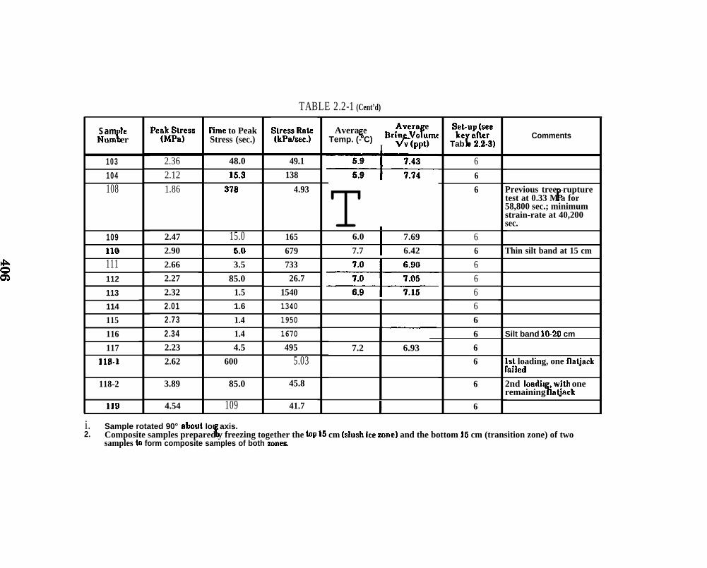
TABLE 2.2-1 (Cent’d)

Avera e

I

.Avera e%Temp. (- C) fBr,~~’p:mf

Sk:u:dSy

rTab e 2.2-3)Sam Ie

[Num erPe~~aess

2.362.12

1.86

I’ime to PeakStress (sec.) Comments

103104108

48.0

15.3

370

49.1

138

6

Previous tree -rupture!test at 0.33 M a for

58,800 sec.; minimumstrain-rate at 40,200sec.

Thin silt band at 15 cm

6

T4.93 6

2.47

2.90

15.0&o

165

679

s6.0 7.69109

1106n

7.7 6.42 6

111 2.66

2.27

2.32

3.5 733

26.7

1540 *

6112

113

114

85.0

1.5

6662.01

2.732.34

1.6 1340115

116

117

1.4

1.4

19501670

6

6 Silt band 10-20 cm

7.2 6.932.23

2.62

4.5 495 6

118.1 600 5.03 6 Ist loading, one tlatjackrailed

118-2

119

3.89

4.54

85.0

109

45.8

41.7

6 2nd losdin with one%-remaining atiack

6

i. Sample rotated 90° about Ion axis.2. tComposite samples prepared y freezing together the tip 15 cm (slush ice zone) and the bottom 15 cm (transition zone) of two

samples to form composite samples of both mnes.

TABLE 2.2-2

RESULTS OF CREEP-RWIVJRE TESTS INUNIAXLAL COMPRESSION -1978,

Time toMin.Str:::cafe 1 Comments

Strain atMinimumStrain rak

Avers e

?$Br” e 01.

v (ppt)

Se#g$re1’Tab e 2.2-3)

Time toRupture (aecl

MinimumStrain rata

Sam ie!Num er

Avera#eTemp (- C)

-

Streaa (MPa)

-

1.66

- 6.76 16

40 9.8 6.34

6.32

6.72

6.85

19

11 9.34 3.8

109.6

11.6

11.610.0

111

Silt &16 cm

)4 Sol19 1.90 70

900820230

296 1.46

1.46

2.34

2.94

17.9 4.79 2

638

20 3.2 x 10-6 18.442

65 18.6

16.0

lB.4

644w x 10”s 8.4 X 10-7 4.9646 0.89 3070 >18,000

1080170

6

4X% 649 2.34

2.99 20 1.4 x lo”~ 1.6 X 10-5 20.6 4.43 6 Siit 10-22 cm,previou8cmp:pr$rsg 0.2

61

62

68,900 sec.2.0 x 10-$1.23

1.17

410 108S $.7 X 10-6 20,020.016.018.9

4.494.52

4.9263 6960

736

9

3.4 x 10-32,2 x 10.s

i.!t X 10-61.6 x 10-6

68 1.66 264 6

8 Siit 10-22 Cmlpreviouscreep tes$0.66 MPa for27,000 sec.

4.4159 2.34 60 400

TABLE 2, 1 (Cent’d)

Minimum Avera e Avera e!

?$

se:-u:~reStrain rate Temp (- C) Br” e 01,

1’Comments

v (ppt) Tab e 2.2-9)

4.1 x 10.s 18.0 4.73 6

7.6 6.76 6

1.1 x 10-4 7.9 6.73 6

9.1 x 10-5 7.1 7.26 6

4.3 x 10-s 7.2 6.95 6

7.4 X 10-6 9.1 6.47 62.6 X 10-5 8.8 6.35 6

1.7 x 10-5 11.1 6.00 6

10.8 6.18 6

4.2 X 10-5 7.5 6.90 6

1.7 x 10-5 7.3 7.16 6 Silt, 10-20cm

5.0 x 10-5 &5 7.78 6 Silt, 5-17 cm2.8 X 10-6 7.0 7,37 68.1 X 10-9 7.0 7.25 69.3 x 10-7 6.9 7.14 69.6 X 10-5 6.5 7.361.7 x 10-8 6.5 7.74 6

Sam le Time to Min.

ENum er Streaa (MPa) strainateStrain atMinimumStrain rate

Time toRupture kc)

I

60 2.62 1 1066 1.72

100 1.1 x 10”386

53 1.8 X 10-367 1.72 I 13

72 1.45 20 140 1.8 X 10-3

EEEE 130245

9.2 x 10-4

1.5 x 10-3

175 2.1 x 10-3

1240683

6.5 X 103■ m

I 82 I 1.19 I

F=lw= 4.2 X 10-34.5 x 10-3

>305716

96 2.01 10

97 1.62 46

37174

1.210-3

1.6 X IO-s

8.5 x 10-498 0.33 3490099 0.85 480100 1.87 15108 0.33 40200

>558003127

49

>58800

1.4 x 10-34.1 x 10-4

TABLE 2.2-3RESUL’1% OF CREEP TESTS IN UNIAXIAL—

TestDurnLion I Avera e

(See) Temp (~C)Avera e

fI

Set-up (see‘ri~’’’p~me key belovd

Sfim IetNum er Stress (MPa)

I

St;::.yk Comments

w0.41 I

*

341

*

n81,900 14.34760.320 I 18.548

Siltzone 10-18cm

50

-+=t-=-

n4.43

I651

636457

69

*

**

7475

-+-i+-80 0,67 I 2.36 X 10-7 97,000 I 10.7

Set-up Key:1. No plastic sheeting on fla .ack~ wooden pegs, 1.3 cm diameter, 20 cm deep.

‘12. Plastic sheeting on IlatJac s; wooden pegs 10 cm deep.3. Plastic sheelin~ on flat]acka; aluminum pegs 1.3 cm diameter. 20 cm deep.4. Plastic sheetin~ on fla~acks; no pegs. - -

h6. No plastic sheeting on a “acks; aluminum pegs 12 cm deep.t6. Plastic sheeting on flatjac s aluminum pegs 12 cm deep.

——

——

——

—

UaN

410

TABLE 2.2-4 (Cent’d)

Averagestress rate(kPdsec)

-

274

5.20

.Avera ef‘r’w’;pim’

4.82

4.78

6.82

Avera e4temp. (- C)Sam le

[NUIU erTime to peak

stress (See) Comments

43 2.87 11,8

12.s6.05.s4.86.0

55044 4.21

2.61

3.16

15

49546

47 61 51.9

S.020.40

6.99

7.40

6.74

48

50

2.111.74

420

4350 Previoustree test at.96 &Pa for28,000 sec.

Low (?k -gasran out

during test

5.9 6.7660 3.92 72 54.4

262

2519.8

3.3

2.7

8.76

9.91

61 4.20

4.27

2.25

16

176263 Low; peak

stress notrecorded

0.15

0.40

15000 10.02

3.02.53.6

3.98 995010900

0.44

9.5064

65 4.37 0.40 10.158.6268 1.76 3960

SampleNumber hlY-

2

3

4

6

a9

1011

1213

14

15

TABLE 2.2-5RESULTS OF CONSTANT LOADING-RATE TESI’S IN

COMPRESSION -1979, MUL’1’i-YEAR* ICE.

4.762.72

1.942.68

4.26

&65

3.63

2.41

2.28

9.69

4.871.50

4.371.67

Time to peakstress (see)

518

4518

503

150.75

69

478456

66

0.599510

163990

Averagestress rats(kPs/see) I

T$:p~$&

I

0.43 11.2

7540 t’--m-

I

5.00 5.5

I

0.43 9.0

Comments

● Salinity <0.2 ppt for all samples.

TABLE 2.2-6RESUL’13 OF CREEP-RUPTURE TESTS IN UNIAXIAL

COMPRESSION -1979

5am Ie Time tomin.

ETime to Strain at Minimum

Streaa (Ml%) drafn rate min. strain Avera estrain rate Br$~~~e Comment9Num er (sec.) rupture (sec.) rate (see-l) Temp. (EC) v

4 1.19 6770 >14460 6.7 X 10”~ 6.23 X 10-7 16.2 4.36

6 0.90 14640 2.2 x 10-3 9.11X108 16.8 4.0697 1.48 840 >6007 2.4 X 10-3 2.18X lox 16.8 4.4298 2.04 220 878 2.9 X 10-5 1.18 X1OS 16.6 4.28

39 2.69 135 940 2.6 X 10-3 1.35 x 10s 19.0 4.11

41 1.79 2384 14.s 4.67

TABLE 2.2-7RESULTS OF CREEP TESTS IN UNIAXIAL

COMPRESSION -1979

Sam leLN u m r

8

14

16

16

46

Stress (MPa) sy~.~~

0.96 4.12 X 10-8

0.86 1.67 x 10-8

0.62 2.41 x 10-8

0.68 2.12 x 10-80.63 6.78 X 10-9

Test Duration

I I

Avers er Avers e(sec.) tTemp. -%3) ‘ r ’ % ’ ’ ; ! - -

76,300 17.6 4.09

202.200 17.6 4.04u m

47,800 17.8 4.22H n

61,300 18.0 4,301 m

147.100 13.9 I 4.72

TABLE 2.2-8RESULTS OF CONSTANT LOMIING, IUI’E ‘IZS’13 IN ~COI@RESSION - 197%

VARIATION WITH DEPTH AND ORIENTATION

l~ading 2col~ Average 3Average

Direction Dep~htnge Peyks:laaa T~~h&m(~ Brine(deg) Number stress rate

(kPa/see) 2V ume

v (ppt)r

0° 1 0-30 3.45 65 53.0 9.3630-60 3.97 76 52.3 9.2660-90 4.05 76 53.3 9.16

o“ 2 0-30 3.54 67 52.8 9.3630-60 4.06 81 50.1 9.26r60-90 4.46 83 53.7 9.16

o“ 3 1545 3.36 66 51.7 9.1945-75 4.49 86 52.2 9.20

75-10s

0° 4 1545 3.41 63 54.2 9.19

45-75 4.07 78 52.2 9.20

75-105 I 4.40 83 53.0 9.3245” 1 0-30 2.66 49 54.3 9.36

30-60 1.81 37 49.0 9.2660-90 2.08 41 50.8 9.16

45° 2 0-30 2.29 45 50.9 9.3630-60 2.34 47 49.9 9.2660-90 2.09 42 49.7 9.16

45” 3 1545 1.99 40 49.6 9.1945-75 1.97 40 49.1 9.20

75-105 2.00 40 50.0 9.3245” 4 1545 1.99 41 48.6 9.19

45-75 2.10 45 46.7 9.2075-105 2.22 44 50.5 9.32

90° 1 0-30 2.91 56 52.0 9.3630-60 3.90 75 51.9 9.2660-90 4.39 81 54.1 9.16

90” 2 0-30 3.42 64 53.4 9.2630-60 3.57 72 49.6 9.2660-90 4.36 76 57.4 9.16

90” 3 1545 3.84 70 54.9 9.1945-75 3.78 77 49.1 9.20

75-105 4.35 81 53.7 9.3290° 4 1545 4.00 73 54.8 9.19

45-75 4.12 74 55.6 9.2075-105 4.48 81 55.3 9.32

1 ~gle between average C.afis Orientation and direction Of load application.QSee Figure for sampling scheme.sAverage temperature -sac fOr d *S=.

414

TABLE 2.2-9RESULTS OF CONSTANT LOADIN(3 RATE TESTS IN

UNIAXiAL COMPRESSION- 1980

Sam le Pe~Jcc;sa Time to peak Average Avera e

[Avera eG %“

sm&t&p?Num er stress (sec.) slress rate

(kPa/sec.] Temp (- C) ‘“%[pp::ne below)

1 2.23 4’/9 4.66 12.3 4.8 1

2 2.52 505 4.99 12.4 4.8 13 9.12 12.4 251 4.8 8.6 24 2.31 476 4.86 8.8 5.6 1

5 2.06 9.0 229 4.1 8.6 2

6 1,87 3.3 568 4.7 8.6 27 2.47 5.2 476 4.7 8.6 29 2.15 427 5.02 19.1 4.6 3

10 2.13 415 5.14 13.1 4.6 311 2.63 54.2 48.5 8.4 5.6 312 2.51 56.8 44.3 8.4 5.6 313 1.73 380 4.56 8.7 5.5 315 1.84 9.75 4.90 8.7 6.5 916 12.9 3480 0.37 3.7 9.7 217 1,22 3387 0.36 3.7 9.7 218 2.38 48 49.5 4.9 8.5 219 2.3S 46 50.2 4.9 8.5 220 3.07 9.8 314 5.2 7.0 4

22 1.84 370 4.97 5.0 8.4 223 2.17 425 6.11 4.9 8.5 2

CommentsI

1 flatjack

Peak stress low, samplecrack ed across onecorner.

1 flatjack

1 flatiack

Load cell operatedluring teat

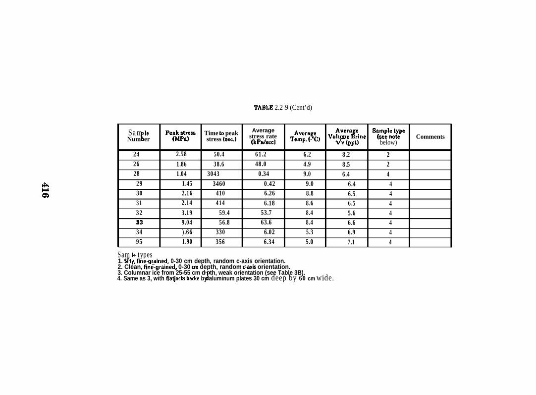
TABLE 2.2-9 (Cent’d)

Sam le\

Pe~~lt:;aa Time to peak AverageT~~p~%$) VoV~~~~ne

Sm#::~peNum er stress rate Commentsstress (Sec.) (kPa/aec) Y below)

24 2.58 50.4 61.2 6.2 8.2 226 1.86 38.6 48.0 4.9 8.5 228 1.04 3043 0.34 9.0 6.4 429 1.45 3460 0.42 9.0 6.4 430 2.16 410 6.26 8.8 6.5 431 2.14 414 6.18 8.6 6.5 432 3.19 59.4 53.7 8.4 5.6 433 9.04 56.8 63.6 8.4 6.6 434 ).66 330 6.02 5.3 6.9 495 1.90 356 6.34 5.0 7.1 4

Sam Ie types“r1. SI ty, fine-grained, 0-30 cm depth, random c-axis orientation.

2. Clean, fine-grained, 0-30 cm depth, random c’axis orientation.3. Columnar ice from 25-55 cm de th, weak orientation (see Table 3B).

t4. Same as 3, with flatjacks backe by aluminum plates 30 cm deep by 60 cm wide.

TABLE 2.2-10 (Cent’d)

45’ 85-115 45 2.4846 2.49

90° 25-55 59 2.3960 2,47

90° 40-70 56 2.6358 2.6377 2.02

78 2.16

90” 66-85 61 2.6862 2.81

90” 70-100 55 2.84n m

I 57 I 2.7490° 85-115 69 2.79

74 2.54

m

53.8 46.0 8.7 4.854.5 45.6 8.6 4.9S2.O 45.9 7.7 5.852.5 47.0 7.7 6.856.4 46.6 9.3 5.357.2 45.9 9.3 5.343.6 46.2 3.6 8.346.8 46.2 3.7 8.158.6 45.8 8.9 5.360.8 46.2 8.9 5.359.0 48.2 9.3 4.958.6 46.7 8.4 5.161.0 45.8 8.6 4.9

56.8 44.7 8.5 4.9

2.2.4.6 Discussion of Results of Uniaxial

2.2.4.6.1 I n t r o d u c t i o n

Compression Tests

The purpose of this section is to present and describe the results of the

experiments listed in the tables in the preceding section. The interpretations are

given strictly in terms of the data and the relevant background material. More

general interpretations in terms of the results of the theoretical study are given in

the appropriate subsections of Section 2.3.

Because the program was done entirely in the field under ambient conditions,

it was obviously not possible to control the temperature or the sample properties.

This leads to some difficulty in organizing the data because the range of variables

examined is limited to some extent. This is because it was generally not possible to

run large numbers of tests at the same temperatures. In general, tests were selected

depending upon the ice temperature on a particular day and the number and types of

tests already done at that temperature. The intent was to assemble the most

complete data set possible within a given temperature range. However, there was no

certainty that temperatures in a particular range would occur often enough to

permit an acceptable data set to be obtained. In addition, it was necessary to

duplicate (or triplicate) some tests in order to establish repeatability so that

variations in sample properties and set-up could be accounted for. This further

reduced the range of variables which could be covered with the available samples.

For these reasons, the results have been grouped into temperature ranges, which are

kept as small as possible while providing a reasonable sample size. This introduces

some scatter into the da-, but the trends are still apparent.

In the following sections data bearing on four aspects of sea ice properties in

uniaxial compression are described. These are (1) the relationship between strength

and stress rate in different temperature ranges, (2) the “long” term strength of sea

ice, (3) the effect of grain size and c-axis orientation on sea ice strength and (4)

comparison of the strength of first year and multi year ice in uniaxial compression.

2.2.4.6.2 ~trengf~ vs. Stress Rate

The results of measurements of strength vs. stress rate in three temperature

ranges are shown in Figure 2.2-8. The data show the anticipated increase of

strength with stress rate (although the scatter is large) as well as the increase in

strength with decreasing temperature. Peak strengths varied from 2.7 h!U?a for the

temperature range from -5.5° to -7.5”C, to about 4.5 MPa for -10° to -14°C to about 6.2

MPa for temperatures between -17° and -22”C.

The strength of 4.5 MPa for the temperature range of -10° to -14°C can be

compared to the peak strengths reached in Wang’s (1979) laboratory tests of the

uniaxial compressive strength of small-scale cylindrical (7.5x 15 cm) samples of

natural sea ice at constant strain rates and a temperature of -lO°C. For fine-grained

(<2 mm) ice, the peak strength was about 7.2 MPa, while for slightly larger grain

sizes (2-3 mm) the peak decreased to about 5.9 MPa. However, for unoriented

columnar ice, Wang found peak strengths of 4.8 and 3.8 MPa for grain sizes of 10 and

15 mm, respectively, which are similar to the value of 4.5 MPa reported above. It is

difficult to draw a conclusion from this, other than to speculate on the possibility

that the strengths reported here may reflect the strength of the ice in the transition

zone of the samples rather than the fine-grained slush ice near the surface.

In experimental programs in which samples are failed at high rates of

deformation, the strength of the ice often appears to decrease at strain rates in excess

of (about) 10-3/sec (the question is discussed more fhlly in Section 2.3.6). No such

decrease in strength is evident in the data in Figure 2.2-8, which raises the question

of whether the stress rates were high enough to reach the peak if, in fact, it is real.

There is no stress-strain law with which to accurately calculate the strain rate.

420

II

iI

II

d

o0.

0~

o“

o.

0:

00

.0P

1

●

●

●

●

●

00

0

o●

✘0

44

o0

●●

a

44

●o0

●

●

421

However, a lower limit to the strain rate can be calculated if it is assumed that the

ice deformed as a linear elastic solid at the higher stress rates. In that case, the

strain rate is related to the stress rate through the derivative of the one-dimensional

Hooke’s law,

t(t) = &(t)m

where E is Young’s modulus. At the higher rates used in this project (say, b = 104

kpahec), for a modulus of 9 GPa, the strain rate would have been on the order of

lo-s/see. This suggests that the data at the highest rates are probably close tO tie

peak and do not contribute to the resolution of the problem.

The variation in failure mechanism over the range of stress rates shown

followed the same pattern for all three data sets. At the lower rates, the ice failed by

the pervasive formation of small, stable cracks which progressively weakened the

sample until it could no longer sustain the load. Samples that were unloaded before

they failed explosively were milky-white, due to the distribution of small cracks. At

the higher rates, the failure always occurred by brittle fracture. Iu some cases the

fractures were through-going extension cracks aligned parallel to the sample axes.

In others, a single vertical shear crack extended across the sample at about 30° to

the axis. In either case, the ice between the main fractures was still clear, with no

small fractures such as were present in samples which were tested at lower rates.

2.2.4.6.3 Long-~erm Strength

Gold (1979) presented data for the time-to-failure of fresh water polycrystalline

ice in constant stress in which, for stresses above some “transition” range, the

samples passed through the inflection point between secondary and tertiary creep in

a relatively short time. Once in tertiary creep the strain rate accelerated until

422

failure occurred. However, the length of time the sample could sustain a stress

without passing to tefiary creep increased rapidly for stresses below the transition.

This suggested the possibility that the ice might have a “fundamental” strength;

that is, an upper limit of the range of stresses which the ice could sustain

“indefinitely” without failing. More recently, Jacka (1984) showed that even at low

constant stresses, the inflection point is ultimately reached, and ice passes into

tertiary creep.

A knowledge of the stress range over which the transition occurs could be

useful for engineering applications. It is not an indicator of a fundamental strength

in the sense defined above. However, it does define a stress below which the ice can

be expected to sustain a load for a relatively long time. In addition, the transition is

of interest for the theory described in Section 2.3.

Data relevant to the question of transition stress are shown in Figures 2.2-9

and 10. The data in Figure 2.2-9 show the time-to-minimum strain rate and time-to-

rupture for tests at constant stress in a relatively low temperature range. In

addition, the time-to-failure for several tests at constant stress rates, and the total

times of constant stress tests which did not reach the inflection point at the

minimum strain rate are also shown. The data show that linear projections of curves

of time-to-failure (for both the constant stress and constant stress rate tests) or time-

to-minimum strain rate must pass through shorter times than those for which the

samples were able to maintain lower stresses without reaching a minimum strain

rate. Thus, the stress vs. time-tu- minimum strain rate curve must flatten as

indicated on the figure, defining the “imnsition” stress. For the data shown, the

transition stress is approximately 1 MPa, and the data indicate that it is sharply

defined.

A similar data set at a higher temperature range is shown in Figure 2.2-10. In

this figure, the minimum strain rate was reached in even the longest tests, although

#Strength-Constant Stress Rate Test5 -

4 -~

Z3 “mm:2 _u)

t -

Constant Stress TestsA Minimum-Strain Ratem Rupture● Steady-State Creep (duration of test )

Average Temp. -f6°C to - f9°CSalinity 5.0 to 5.5 Yoo

o~IXIO1 IX102 IXI03 txloq IX105 1X106

TIME (SEC)

Figure 2.2-9 Uniaxial compressive strength vs. time-to-failure for constant stressrate tests and time-to-minimum strain rate and time-to-rupture atconstant stress in the temperature range -10° to -19°C.

it was not possible to hold the loads on the samples until rupture. The curves

through the data points are estimates (their shapes reflect the results discussed in

Section 2.3.4). The transition is less well defined in this figure, because the slope of

the stress vs. minimum strain rate curve is low compared to that in Figure 2.2-9.

However, a value of 0.5 MPa might be a reasonable estimate.

In general, samples which ruptured at constant stress failed by the pervasive

growth of small cracks, which gave the ice a whitish color. Few cracks were ever

observed to form in samples tested at stresses below the transition stress.

It is of interest to note that for constant stress tests, the time- to-rupture is

usually between a factor of 3 and 10 greater than the time-to-minimum strain rate,

with a tendency to increase at lower stresses. Similar data for ice in bending would

424

I 1 I I I 1 I I 11111 8 I 1 I I 1111 I I I I IIIIJ I 1 I I 11-

0

: q1 1 I I I 1 I I 11111 I I I I 11111 1 I I 1 11111 1 1 1 1 11{

. - 10 100 1000 10,0005 t (See)

Figure 2.2-10 Uniaxial compressive strength vs. time-to-failure for constant stressrate tests (open circles), and time-to-minimum strain rate (solidcircles) and time-to-rupture (solid triangles) for constant stresstests. Temperature range -5.5° to -7.5°C. Curves are estimatedbased on the results in Section 2.3.4.

have application to the problem of the length of time for which an ice sheet can be

expected to safely bear a load.

2.2.4.6.4 Effect of Grain Size and C-Axis Om”entation on Strength

Peyton (1966) and Wang (1979) both demonstrated the effect of strong

alignment of crystallographic c-axes of crystals in an ice sheet on the stiength of the

ice loaded in various orientations. In this study, similar measurements were made

to include the effect of depth (and therefore increasing grain size). To accomplish

this, samples were collected in 30-cm increments of depth down to 105 cm in the ice

sheet (Figure 2.2-11). These were oriented so that loading could be done at 0°,45° and

90° to the dominant c-axis direction on two samples collected for each orientation and

depth interval. The study was first done in 1979 and was repeated in 1980 in an

effort to collect data over a different temperature range. The results of the 1979

program are shown in Figure 2.2-12. Loading was done at a stress rate of about 52

kptisec (7.5 psi/see) which was similar to that used by Peyton (1966) in his work on

425

PLAN VIEW

Dominant C-Axis Direction

Do

90” 45°

C R O S S - S E C T I O N~ Datum,3

n

Wvm-

3 0

6 0

9 0 El3

5 H2

4

6

Samples 1-6

awa

Figure 2.2-11 Arrangement of samples collected for evaluation of uniaxialcompressive strength vs. grain size and c-axis orientation.

ice strength as a function of grain size and c-axis orientation. Average sample

temperatures during testing were -3°C ( +-/- 0.5”C).

The results of the 1979 study agree with those of Wang (1979) with respect to

the increase of strength with depth for the 0° and 90° orientations. However, they

contrast with the results of both Wang (1979) and Peyton (1966) which show that the

strength in the 0° direction is greater than that in the 90° direction. There maybe no

discrepancy with respect to Wang’s results because, at the loading rate used in this

program, the sample strain rates would probably have been in the range of 10-%ec

to 10-Vsec. At those rates, the difference between the strength in the 0° and 90°

directions in Wang’s (1979) data are small and possibly within the scatter of the

results in Figure 2.2-12.

426

.

b

■

m

❑

A

. 0° Loading Direction

. 900 41 II

A 45° Loading Direction

A

$

A

AA:A

A

I I I I I !O !5 30 45 60 75 90

DEPTH (CM)

Figure 2.2-12 Results of the 1979 series of tests of uniaxial compressive strengthvs. grain size and c-axis orientation.

It is likely that the discrepancy is real with respect to the data in Peyton

(1966) but, if SO, the same discrepancy exists between Wang’s and Peyton’s results.

In this case, the lack of agreement maybe due to the differences in the volume of

the samples used in the three studies.

Peyton’s tests were done on samples about 3.5 cm in diameter by 7 cm long. For

depths greater than about 30 to 60 cm in an ice sheet (particularly when the c-axes

are strongly oriented), samples of this size are probably closer to single crystals of ice

than to polycrystalline ice. For the 90° orientation, the brine planes in the ice were

aligned parallel to the sample axis. Thus, when loaded in uniaxial compression, the

brine planes were properly oriented to nucleate extension fractures which, in a large

sample might have been trapped at the grain boundaries and stabilized. However,

427

for Peyton’s small samples their size would have been significant compared to the

length of the sample, leading to weakening and premature fracture. In contrast, the

samples used by Wang (approximately, 7.5 x 15 cm) and in this study, were large

enough that the grain sizes were insignificant in comparison to the sample

volumes. Thus, small cracks parallel to the brine planes would have stabilized,

increasing the stress required to cause failure.

Note that for the 45° direction the strength decreased with depth initially, and

then remained constant (within the scatter) despite the increase in grain size with

increasing depth. An interpretation is suggested by the observation that, with the

exception of samples including the slush ice layer, failure in samples with this

orientation always occurred by shear fracture at 45° to the sample axis. Thus, the

fracture plane was always parallel to the orientation of the brine planes and in the

plane of maximum shear stress. This implies that once the orientation was

sufficiently strong for sliding to occur easily in the direction of orientation of the

brine planes, further intensification of the orientation had little effect on the

strength.

The results of the test series in 1980, in which the same test program was

repeated at average sample temperatures of -7 to -9°C “are shown in Figure 2.2-13.

These data indicate little or no variation in strength with depth or loading direction

relative to c-axis orientation. The results of additional tests at -3°C, which were run

to check the results of the first series, also indicate no difference in strength between

the 45° and 90° directions (Figure 2.2-13). The apparent reason for the absence of

any particular orientation effect in these results is that the orientation was simply

not developed strongly enough. There is no question that the ice tested in 1980

should be classified as “orien~d,” because an average c-axis orientation could easily

be identified in thin sections of the ice. However, thin section analysis showed that

in 1979, the ice at a depth of 32 cm had a maximum angular spread between c-axes of

428

Soiid Symbols Temp.-7°C to 9°COpen Symbols Temp. -3° C

● 0° Loading Directim● 90* la u● 45° Loading Direction

A

A

9A

A8 a

●

30 45 60 75 90 {05DEPTH (CM)

Figure 2.2-13 Results of the 1980 series of tests of uniaxial compressive strengthvs. grain size and c-axis orientation.

about 30°, decreasing b 15° at 1 m. In contrast, in 1980, the angular spread was up

to 66° at a depth of 75 cm. This large variation was apparently sufficient to

neutralize the effect of the average c-aws orientation, with the result that the ice in

1980 was essentially isotropic for loading in the horizontal plane. This result

indicates that there is some limit in the degree of orientation (i.e., some maximum

permissible spread of c-axis orientation) which is required before the ice will exhibit

mechanical anisotropy for loading in a horizontal plane. The fact that an average c-

taxis orientation can easily be identified in a sample does not assure that such a

mechanical anisotropy exists.

429

2.2.4.6.5 Compam”son of the Strength of First Year and Multiyear Ice

A series of tests was run to provide a comparison between the strength of first

year and multiyear sea ice in uniaxial compression at the same temperatures and

loading rates. The samples of multiyear ice were collected from a floe frozen into the

landfast ice sheet near the test site. Average ice temperatures ranged from -2° to -6°C

during the test program. Tests at each stress rate were run consecutively,

alternating between the two ice types. The results are shown in Figure 2.2-14 and

indicate that there is little difference in strength between the two ice types, except

possibly at the highest rate at which tests were conducted. This suggests that the

strength of multiyear ice maybe greater than that of first year ice in the brittle

range, but there is little difference over the remainder of the range of loading rates

used.

●

0●

0

0

●

00

TEMPERATURE -2°C tO - 6°C? o First Year Ice

● Multi-year Ice

0.!

Figure 2.2-14

i.o sTR~s:iRATE (k;%:c)IXI03 IXI04

Uniaxial compressive strength of first year and mdtiyear icevs. stress rate.

430

2.2.5 DIRECT SHEAR TESTS

A direct shear test (which is similar to a standard “shear box’* test) was

designed, and several preliminary experiments were run. The values are not

reported here because the flatjacks used for loading were not calibrated. However,

the test results were repeatable, and the procedure could form the basis for a test

program to evaluate the shear strength of sea ice. Details were described in Shapiro

et al. (1979) and are only summarized here.

The configuration of the testis shown in Figure 2.2-15. The sample is defined

by the relief slots which are cut h the depth “a” with a chain saw. The testis done by

loading the flatjack until failure occurs along the plane at the base of the block. The

shear strength is then calculated assuming that the stress is uniformly distributed

on the failure plane, as is done in the case with shear box experiments. Thus, if the

dimensions of the flatjacks are a and b, and the (calibrated) flatjack pressure at

failure is P, then the total force is Pab. This is assumed to be equal to z bc, where ~ is

the shear strength, and b and c are the dimensions of the block in the plane of the ice

sheet as outlined by the relief slots. In the tests done during the program, b and c

were equal, so that t = (tic)P. Experiments were done with the ratios W and a/c

equal to both 1/2 and 1/3, which gave similar values of z.

The geometry of the stress distribution in the test block was studied using a 2-

dimensional plane stress, finite element analysis. The results were compared to

similar calculations for the geometry of a punch test (Figure 2.2-16) which is oftin

used to determine the shear strength of materials. The calculations indicate that the

first crack to form in the shear test would likely be a tension crack propagating

downward under the flatjack into the ice sheet. Subsequently, the stress

configuration near the flatjack closely resembles that of the punch test as shown in

Figure 2.2-16. The vertical crack can be simulated at the time the testis setup by “

deepening the chain saw cut made to receive the flatjack and installing a piece of

Relief Slot

IL Ice Surface/)

*==--.=: .-.== z =+=-=-.-=.---.75/: -.-s::; 7

IceSurface

Trrb--- 1. . . . . . . ..- --------. + ,“

-----: . . . . . . ..- . . . . . . . . . --.Z .A~

Relief Slot Cross Section

Figure 2.2-15 Set-up for direct shear test.

stiff cardboard wrapped in polyethylene sheeting in the slot below the flatjack. This

would provide a low tensile strength bond, assuring that the first crack will

propagate downward.

Examination of the fracture zones which formed on the sheai plane as a result

of the tests, shows that the zones were generally thin, involving only the lower 20%

of the thickness of the blocks. Within the zone, the ice tended to shatter into flat

plates about 1 cm thick, with linear dimensions of several centimeters. The ftilure

plane in the ice sheet typically showed irregular “step” asperities oriented

transverse to the direction of motion of the failed block, with the riser of the step

facing the loading direction. Flat cracks extended down into the ice from the base of

each step, as evidenced by the distinct gray color of the ice in these areas. The failure

mode was similar to that in the fracture zone of rocks which fail in shear by brittle

fracture in uniaxial compression. The mechanism clearly indicates failure under the

influence of a shear stress parallel to the failure plane.

432

Punch—

P-

o.5P- ~ - - - - - - - - --- .-4~z~, 0“&

‘%-P- \\

\ ,

Figure 2.2-16

1 \ !

. . . —

Results of finite element analysis of punch test (solid line) anddirect shear test (dashed line). Calculations refer to a surfacejust below the dashed lines on the diagrams. The slot belowthe flatjack represents either the first crack or the prepared“crack” described in the text.

It should be noted that attempts to conduct direct shear tests using square

flatjacks and blocks with dimensions a = b = c invariably resulted in tensile failure

across the base of the specimen. Thus, cubical blocks simulate the bending of a thick

cantilever beam under a uniformly distributed load. However, tests in which the

width of the flatjack was at least twice the depth always failed in shear.

Finally, note that the test described above can be used to determine the shear

strength of the ice in any direction. This would involve quarrying samples from the

ice sheet, rotating them into the desired orientation, and then freezing them into

holes prepared in the surface of the ice sheet. A sample need only be large enough

that the set-up shown in Figure 2.2-15 can be made on its surface.

4 3 3

2.2.6 INDIRECT TENSION (BRAZIL) TEST

A procedure for running indirect tension tests in situ in the ice sheet was also

tried (Shapiro et al., 19791. Only two tests were required to duplicate failure

patterns obtained in the laboratory. In the first of these, a circle with a diameter of

59 cm was outlined on the ice surface and two 15-x 60-cIn flatjacks were installed on

the opposite ends of one of its diameters; the 15-cm edges of the flatjacks were at the

surface of the ice sheet. A chain saw cut 75 cm deep was made along the

circumference of the circle, and the flatjacks were then loaded until failure occurred.

The cylinder failed with a single crack along the diameter and minor secondary

cracks near the flatjacks. This is the typical mode of failure in laboratory tests of

this type when the cylinders are loaded by line loads on opposite ends of a diameter.

Curved flatjacks were used in the second test, in order to provide a load over 15”

arcs of the test specimen as discussed by Jaeger and Cook ( 1976). The purpose of

loading over the arc is to eliminate the secondary cracking near the points of

application of the line load, and assure that failure occurs along a single fracture

which originates near the center of the sample. The sample used for this test was

another cylinder of the same size as in the first test (diameter 59 cm, depth 75 cm).

The flatjacks were prepared by flattening two 46 cm lengths of 7.6 cm diameter

copper tubing, and then bending them to the curvature of the test specimen. The

ends of the flatjacks were sealed by silver soldering, with inlets for loading installed

atone end. The test was set up and run as described above, but in this case failure

occurred along a single crack with no secondary cracking near the flatjacks. Further,

when the sample was cut normal to the crack with a chain saw, it separated into two

blocks along the crack. There was no evidence of splaying of the crack with depth in

the ice sheet, which indicates that plane strain conditions were achieved over a

sufficient length of the sample to provide an adequate test.

434

The results show that large-scale, in situ indirect tension tests are relatively

easy to setup and run. and failure mechanisms duplicati those which typically occur

in laboratory tests. Thus, there should be no difficulty in conducting a larger

program of tests of this type if the results were needed.

2.2.7 BIAXIAL COMPRESSION TESTS

Experiments were done to develop a biaxial compression test using rectangular

prisms of sea ice of the same dimensions as those used in the uniaxial compression

tests (Shapiro et al., 1979). The tests differ only by the addition of a confhing

pressure applied through 30=x 6(km flatjacks installed along the sides of the

samples. The confining pressure was controlled by a loading system which was

separate from that used to apply the loads to the ends of the sample.

The tests were done by loading both pairs of flatjacks simultaneously, until the

selected confining pressure was reached. Then, the pressure in the confining

pressure flatjacks was held constant, while the pressure in the flatjacks at the ends

of the sample was increased at a constant rate until failure occurred.

The results of the experiments indicate that this testis likely to be useful only

when the ice temperature is low and the loading rate of the axial flatjacks is less

than 0.35 Ml?a/sec (50 psi/see). The limitations are due to the increase in the

strength of the samples with application of confining pressure. This allows the

pressure in the axial flatjacks b become so large that the ice sheet (the “loading

frame”), which is not under confining pressure, is not sufilciently strong to resist the

expansion of the flatjacks under internal pressure. As a result, the axial flatjacks

fail along the edge weld at the ice surface as the flatjack overexpands.

Additional work in progress when the field progrsm was terminated was

directed attesting the use of aluminum or steel plates installed behind the axial

flatjacks to spread the load and reduce the stress applied to the ice sheet by the

435

reaction pressure. A few experiments run under these conditions suggested that the

approach might lead to an increase in’ the range of pressures over which tests could

be done.

Since the procedure was never developed to the point of running a series of tests

to obtain numerical values of the strength, the flatjacks used to apply the confining

pressure were not calibrated. For the limited data obtained, the results suggest that

the increase in peak axial stress with increase in confining pressure is strongly

dependent on both the temperature and the rate of loading. In addition, it was never

possible to bring a sample to failure by the development of through-going cracks,

although a few tests were done at rates which, for uniaxial compression, would have

caused failure by that mechanism. Instead, cracking was always pervasive, turning

the sample milky-white, as occurred in uniaxial compression tests at low loading

rates (Section 2.2.4.6.2).

The procedure as described above could be used for conducting creep tests at

low flatjack pressures, but further development is required if the testis to be used to

establish the strength at higher rates of loading and confining pressures.

2.2.8 SUMMARY AND DISCUSSION

The physical properties of sea ice, and its mode of occurrence in nature require

that at least some determinations of the mechanical properties of the ice must be

conducted in situ in order to supplement laboratory results. In situ tests involving

vertical loading of an ice sheet (or of beams isolated within an ice sheet) had been

done previously, but the problem of testing under in-plane loading had received little

attention prior to this program. Therefore, one task was to investigate methods

through which the properties of sea ice could be determined on relatively large

samples under conditions of in-plane loading, and with minimal disturbance to the

samples being tested.

436

Flatjacks proved to be ideal devices for introducing controlled stress fields into

an ice sheet. They are relatively simple and inexpensive to construct in any shape,

and can be adapted to a variety of test types. Loading by high pressure gas controlled

by a pressure regulator proved to be satisfactory for tests at both constant load and

constant loading rate. For the latter, rates ranging from less than 1 M?tisec h

greater than 104 M%./sec were achieved.

Deformation measurements can be made using a variety of equipment but are

limited by the fact that, in the tests described here, only the face of the sample at the

ice surface can be instrumented. The result is that as the sample surface bulges

upward in response to the in-plane shortening, the measured strain on the single

exposed face ceases to be representative of the true shortening. The method of

attaching displacement measuring devices to pegs in the ice overcomes this difficulty

to some extent, but introduces the question of whether the pegs tiect the

deformation characteristics of the ice. The results presented here suggest that it is

possible to determine the conditions under which this does not occur. However, it

would still be desirable to verify the validity of the strain determinations by other

methods.

During the program, procedures for conducting tests in uniaxial compression

(triangular and prismatic specimens), direct shear and indirect tension were

designed and tested with satisfactory results. A biaxial compression test was also

tried. It is adequate for creep tests or for measurements of strength at low conilning

pressures (i.e., less than about 20% of the peak axial stress), but requires further

work if it is to be extended to higher confining pressure.

The data on uniaxial compressive strength as a function of loading rate follows

the same trend of increasing strength with increasing rate as established for

constant deformation rate tests. There is no stress- strain law available with which

to correlate between test types. However, estimates suggest that the data presented

here are comparable to those obtained by Wang (1979) on smaller samples, irnpl@ng

that there is no marked decrease in strength with increasing sample dimensions for

samples in which the c-axes are not strongly oriented.

The results of tests at constant stress verify that some transition stress range

exists for sea ice, below which the time that the ice can sustain a load increases

rapidly. The transition is defined by plots of stress vs. time-to-minimum strain rate

(the onset of the tertiary creep stage leading to rupture) for a series of tests. The data

indicate that the transition is sharp at low temperatures but becomes more gradual

as the temperature increases. The recognition of the transition range may have

engineering applications by defining the upper limit of the stress which the ice can

sustain for a relatively longtime. In addition, while any sample under load must

eventually fail, the data indicate that the time between the inflection point and

rupture of the sample is from 3 to 10 times as great as the time-to-minimum strain

rate. This may provide a basis for deriving safety factors for loads on ice sheets.

A series of determinations of sea ice strength as a function of depth in the ice

sheet (or, alternatively, grain size) and c-axis orientation follows trends indicating

strong mechanical anisotropy of the ice. The tests were done on strongly oriented

ice, and the trends are similar to those derived in laboratory measurements.

However, the results of a second series of tests raise the question of the intensity of c-

taxis orientation which is required in order for the anisotropic effects to become

important. In that series, the intensity of c-axis orientation of the ice was weaker

than that in the first series, but still strong enough to be easily recognized. The

results showed that the ice was essentially mechanically isotropic for loading in the

plane of the ice sheet, implying that there is a relatively sharp transition from

isotropy to anisotropy as the intensity of c-axis orientation increases.

438

Finally, a short series of measurements was done to compare the strengths of

first year and multi-year ice. The results showed no significant differences over the

range of loading rates and temperatures used in the experiments.

2.2.9 REFERENCES CITED

Croasdale, K. R. (1974) Crushing stiength of Arctic Ice; in Coast and Shelf of the

Beaufort Sea, Proceedings of a Symposium on Beaufort Sea Coast and Shelf

Research, J. C. Reed and J. E. Slater, eds., Arlington, Virginia, Arctic Institute

of North America, PP. 377-399.

Groasdale, K. R., Morgenstern, N. R. and Nuttall, J. B. (1977) Indentation tests to

investigate ice pressures on vertical piers; Jour. Glac., v. 19, no. 81, pp. 301-

312.

Deklotz, E. J. and Boisen, B. P. (1970) Development of Equipment for determining

deformation modulus on in situ stress by means of large flatjacks; in

Determination of the In Situ Modulus of Deformation of Rocks, ASTM STP 477,

pp. 117-125.

Gold, L. W. (1979) The process of failure of columnar-grained ice; Phil. Msg., v. 26,

no. 2, pp. 311-328.

Jacka, T. H. (1984) The time and strain required for development of minimum strain

rates in ice; Cold Regions Sci. and Tech. v. 8, pp. 261-268.

Jaeger, J. C. and Cook, N. G. W. (1976) Fundamentals of Rock Mechanics, 2nd cd.,

Halsted Press, New York, pp. 585.

Peyton, H. R. (1966) Sea ice strength; Geophysical Inst. U. of Alaska-Fairbanks

Report UAG R-182, pp. 273.

Pratt, H. R., Black, A. D., Brown, W. S. and Brace, W. F. (1974) A new technique for

determining the deformation frictional characteristics of in situ rock; in Field

Testing and Instrumentation of ~ck; ASTM STP 554, pp. 3-19.

4 3 9

Shapiro, L.H. and Hoskins, E. R. (1975) The use of flatjacks for the in situ

determination of the mechanical properties of sea ice; Proc. 3rd Conf. on Port

and ocean Eng. under Arctic Conditions, Fairbanks, Alaska, pp. 427-436.

Shapiro, L. H., Hoskins, E. R., Nelson, R. D. and Metzner, R. C. (1979) FlaQack

methods of in situ measurement of the mechanical properties of sea ice; Trans.,

A. S.M.E., Jour. Energy Resources Tech., v. 101, pp. 1996-2002.

St. Lawrence, W. F. and Cole, D. M. (1982) Acoustic emissions from polycrystalline

ice; Cold Regions Sci. and Tech. v. 5, pp. 183-199.

Wang, Y. S., 1979, Crystallographic studies and strength tests of field ice in the

Alaskan Beaufort Sea; Proc. 5th Conf. on Port and Ocean Eng. under Arctic

Conditions, Trondheim, Norway, pp. 651-655.

Weeks, W. F. and Assur, A. (1967) The mechanical properties of sea ice; USA CRREL

Cold Regions Science and Engineering, Part II, Section C, pp. 80.

Weeks, W. F. and Gow, A. J. (1978) Preferred crystal orientations in the fast ice

along the margins of the Arctic Ocean; USA CRREL Report 78-13.

4 4 0

2.3 A STRESS-STRAIN IAW AND FAILURE CRITERION FOR SEA ICE

by

Lewis H. Shapiro

ABSTRACT

The objective of this section is to describe the reformational behavior of the

spring-dashpot model of a 4parameter viscoelastic fluid constrained to fail according

to the distwtional strain energy density criterion. The results predict upper and

lower strength limits for the model, and permit curves to be derived which show the

relationships between the results of hypothetical tests on the models at different

loading paths and rates. Comparison of the analytical results to experimental data

for sea ice and polycrystalline fresh ice shows that the trends of the curves are

similar and that the strength limits may correspond to transitions in deformation

mechanisms. This suggests that the combination of a more realistic non-linear model

with the failure criterion could provide an accurate description of the stress-strain

relations and failure of ice under a range of loading conditions.

2.3.1 INTRODUCTION

A program of evaluation of previous work on the strength and”mechanical

properties of sea ice was conducted along with the experimental work described in

the last section of this report. The objective was to identify and characterize the

reformational behavior of sea ice, with the intent of using the results to indicate a

possible form of a stress-strain law and failure criteria for sea ice. Since most of the

available data are for loading in uniaxial compression (as are the results reported in

Section 2.2.4.5), the law was to be restricted to deformation in that loading mode.

However, examination of the published data for tests in other loading modes

suggests that the results may be applicable to some of these as well.

441

It is well known from experimental work that, for uniaxial compression tests,

most types of ice follow the same basic patterns of response to load. In general, the

strength and rate of deformation are non-linearly related to the load (in cons-t

load tests) or to the rate of loading (in constant load rate or constant deformation rate

tests). This is certainly true for sea ice, as shown by the data in the last section and

by the review of the literature. In addition, as has been previously noted (see, for

example, Mellor, 1980), the stress-strain curves for ice are qualitatively similar to

curves calculated for the response to load of the model of a linear 4-parameter

viscoelastic fluid (4-PF). This suggested that the stress-strain law for a 4-PF with

non-linear elements might provide realistic curves tQ match the data. Accordingly,

a series of stress-strain calculations were done for such a 4-PF model, and the work

was extended to consider the case where the model is constrained to fail under the

distortional strain energy criterion (DSEC). The results qualitatively predict the

relationships between tests along different loading paths and also provide a basis for

explaining many of the results of experimental programs. In addition, they lead to

suggestions for further experimental work.

The stress-strain law for the 4PF model with non-linear elements is

cumbersome and requires numerical values of the parameters for calculation of the

curves, so that it is difficult to generalize the results. In order to permit

generalizations to be made, and to exsmine the details of the behavior of the

combined 4-PF and DSEC model, it is preferable to use the model with linear

elements for which most-of the derivations can be done in closed form. The

presentation and discussion of the results of that work in terms of available data is

the subject of this report.

The remainder of this section is divided

istics and justification for the use of the 4-PF

in Sections 2.3.2 and 2.3.3, respectively. They

4 4 2

into five subsections. The character-

model and the DSEC are described

are then combined in Section 2.3.4

and the conditions for yield of the model under different loading programs are

derived without reference to experimental results. There are two reasons for this

approach. First, as noted above, the stress-strain laws for the elements in the model

are taken to be linear. This permits most of the derivations and proofs to be done in

closed form rather than numerically, which is convenient for qualitative comparison

between the deformation of the model and the available data. However, the results

of this analysis cannot be applied quantitatively h the non-linear behavior of sea ice.

The results of calculations based on the non-linear model are shown for comparison,

to illustrate that the trends of the relationships are independent of the form of the

laws. However, the results of this section are intended to be interpreted

qualitatively.

The second reason is to emphasize the fact that the model is simply a

mathematical device which may (or may not) represent the response to load of a real

material over some range of conditions. In effect, it is a mathematical entity which

is independent of any data set. Its utility for describing the reformational behavior

of a real material depends upon the extent to which the calculated deformation of the

model and the actual data agree. There is no a priori reason to expect these to agree

over any, or all, of the possible ranges of the variables; the degree to which they

correspond is a matter to be determined from examination of the data. The model

responses are discussed in terms of imaginary experiments on some ideal material

which the model represents. This is done so that uncertainties which arise in

experimental programs can be included in the interpretation of the calculated

results.

The results of the calculations are compared to the data on different ice

types in Section 2.3.5. This section relies heavily on the data for sea ice presented

in Sections 2.2.4.5 and 2.2.4.6, and on data from Hawkes and Mellor (1972),

Mellor and Cole (1982), and Jacka (1984) on polycrystalline fresh ice.

The summary, conclusions, and suggestions for ftiher work are given in

Section 2.3.6, which is followed by an appendix (Section 2.3.8) where the details of

the derivations appear.

In the equations which follow, the symbols o for stress and c for strain are

assumed to be functions of time. They are written as shown in the interest of brevity.

A dot over a time-dependent variable indicates the time derivative, and a zero

subscript always defines a constant value (i.e. co is a constant strain rate; U. is a

constant stress). The “constants” used in the model are constant with respect to

stress and strain, but would be expected to vary with the temperature and physical

properties of the medium they represent. That variability is not considered here.

2.3.2 DESCRIPTION OF THE 4-PARAMETER FLUID MODEL

The justification for the use of the 4PF model follows from the assumption

(commonly used in the analysis of deformation experiments on ice and other

materials) that the total deformation includes elements of instantaneous elastic

response to the applied load followed by both time-dependent elastic and plastic

behavior. Thus, the tdal stiain is often represented by the equation

(1) &’r = c~+cv+c~

where CT, CE, cv and CD are the total strain, “instantaneous” elastic strain, time-

dependent elastic strain and time-dependent plastic strain, respectively. Equation

(1) represents the response to load of the spring- dashpot model of a 4PF (shown with

linear elements in Figure 2.3-1) consisting of Voigt and Maxwell models connected

in series. This is the simplest of the spring-dashpot models that contains all of the

elements of a creep curve. The spring of the Maxwell model gives the

“instantaneous” elastic response to an applied load while the viscous creep of the

dashpot of the Maxwell model at constant stress represents the summation of the

contributions of the mechanisms which produce time-dependent permanent

deformation in actual materials. The Voigt model provides a time-dependent elastic

response which, in a creep curve, gives the decrease in strain rate with time through

the primary creep stage and the time-dependent recovery of strain in the recovery

stage following release of the load. Sinha (1979) suggested that grain boundary

sliding is the mechanism which is responsible for this behavior. The use of the Voigt

model here is justified by Hart et al. (1975) based upon experimental data from

metals. They argued that the data require that the stress-strain relationship for

delayed (time-dependent) elasticity is of the form

(2) ; = f[u-Mc]

where 3 is the strain rate and u is the applied stress. The parameter M is defined as

the “saturation” modulus and is found from the equation

M = (J~&M

when ~ goes to zero and the strain reaches its maximum value CM at the transition

from primary to steady state creep in a test at constant stress. Equation (2) is simply

the form of the stress-strain law for a Voigt model (Flugge, 1967) in which M

corresponds to the modulus of the spring kz in the 4-PF model (Figure 2.3-l).

Voigt Model Maxwell Model

7?*

/ 1

tcJ

+Crl

$ 1—~+ty/ 4+-CT* w, k,

k 2

Figure 2.3-1 Spring-dashpot model of a 4-parameter linear viscoelasticfluid. kl and kz are spring constants, ql and qz are theNewtonian viscosities of the dashpots. al and 02 show thepartitioning of the applied stress a across the arms of theVoigt model, such that u = U1 + uz (see text).

4 4 5

Equilibrium of the stresses across the Voigt model (Figure 2.3-1) requires that

o =UI+U2

so that, for the linear case, the strain and strain rate are

where qz is the coefficient of Newtonian viscosity. Thus, the stresses, strain and

strain rate of the Voigt model are related by the equilibrium condition at any stage

in the loading path.

An important limitation on the ability of the 4-PF model to predict the response

of actual materials follows from the form of equation (1) in which the contributions of

the mechanisms which produce each of the types of response to load described above

are added linearly. This is equivalent to the assumption that the elements do not

influence each other in the sense that, for example, the magnitude of deformation

due to time-dependent plastic flow mechanisms does not lead to changes in the

values of the parameters which govern other types of deformation. It seems likely.

that this assumption must fail at some point in the deformation process, but the

subject has not been investigated.

The parameters of the linear form of the 4-PF model have been determined for

polycrystalline fresh ice from creep tests in tension (Jellenick and Brill, 1956) and in

uniaxial and biaxial compression (Lindgrin, 1970), and for young sea ice in

compression and bending (Tabata, 1958). Nevel (1976) used this stress-strain law in

a theory of the creep of floating ice sheets. Stress-strain laws which are similar to

the 3-or 4-parameter viscoelastic model have been applied to ice by Maser (1972)

and Sinha (1978). The general application of these types of laws to ice has been

discussed by Mellor (1980).

4 4 6

Note that there is no requirement that the elements of the model in Figure 2.3-

1 be lineu, non-linear elements (both springs and dashpots) have been used by

different authors to describe the deformation of different materials. Hutter (1980)

pointed out that only the hyperbolic sine law for steady-state creep is based on a

theory of material behavior, the rate process theory [Glasstone et al., (1941); Krausz

and Eyring, (1975)]. Commonly, the hyperbolic sine law is used for the dashpot of

the Maxwell model in Figure 2.3-1, as in the non-linear stress-strain rate law for

creep

9& = A (sinh Qo)n.

However, it has also been used for the dashpot of the Voigt model in the application

of the stress-strain law of a 3-parameter viscoelastic solid to polymers, rubber and

textiles (Krausz and Eyring, 1975, and references cited therein). The non-linear law

considered earlier in this project (and described in the appendix) involved the use of

the hyperbolic sine law for both dashpots. Other workers have used other

combinations of linear and non-linear elements. This is permissible, provided that

the contributions of the model elements add as shown in equation (l).

For any stress-strain relations of the individual elements, the 4-PF model

yields a differential equation which can be integrated for any loading path. The

discussion here will be restricted to the paths commonly used in experimental

programs; constant stress (CS), constant stress rate (CSR) and constant strain rate

(CDR). The curves from the integrated equations for these paths for the linear model

are shown in the appendix. They are qualitatively similar to experimental curves for

ice up to the point of failure (see, for example, the discussion in Mellor, 1980).

The parameters of an ideal linear material represented by a 4-I?F model can be

determined from the results of a single creep test. More creep tests would be

required in order b determine the form of the stress-strain law for the dashpot of the

Maxwell model of an ideal non-linear material.

4 4 7

Given that law, the form of the laws

for the elements of the Voigt model can be found. However, these determinations

assume that the material is in steady state creep, as required by the definition of

the “saturationn modulus. As discussed in Section 2.3.5.2, this condition is

probably never reached in experiments on ice. Thus, there is a question as to the

significance of the parameters reported in the references cited above. The point is

discussed in Section 2.3.5.4.

2.3.3 DESCRIPTION OF THE DISTORTIONAL STRAIN ENERGYDENSITY YIELD CRITERION

Reiner and Weissenberg (1939) suggested the idea of applying the DSEC to

spring-dashpot models, and Reiner (1960) demonstrated the results for the 3-

parameter linear viscoelastic solid. The extension to the 4-parameter model follows

directly. Day (1975) has given a general proof that the application of the DSEC to

models of this type is valid without restriction to elements with linear stress-strain

laws, provided that the model elements do not influence each other, in the sense

described above.

The DSEC is based upon Von Mises’criterion expressed in terms of the strain

rather than the stress (Reiner, 1960). The work done by the applied stress in

deforming the dashpots of the model is assumed to be dissipated through internal

friction, while that done on the springs is stored as distortional elastic strain energy.

Yield is assumed to occur when the stored distortional strain energy reaches the

resilience, “R”, the energy (per unit volume) required to deform an elastic body to its

elastic limit.

Note that while Von Mises’ criterion was derived to predict yield (the onset

of flow) of plastic materials, it has also been used as a fracture criterion for ice,

rock, and other materials (as in Section 3.1). For the remainder of this work, the

general term “failure” is used in place of “yield” since, as shown below, the DSEC

appears to apply to experimental results over the range from ductile to true brittle

behavior.

Von Mises criterion is expressed by the equation

J2 = K2,

where Jz is the second invariant of the stress deviator tensor and K is the shear

strength of the material represented by the model. Assuming the material to be

elastically isotropic, for uniaxial loading at a stress IS, following Mendelson (1968)

J2 = (1/3)02

and the distortional strain energy is

Ud = (1/6G) U2 = (1/2G) J2

where G is the shear modulus. Then, from Reiner (1960) the distortional strain

energy of the 4-parameter model is simply the sum of the strain energies stored in

the two springs. Failure occurs when

(3) Ud = R = kl(tE)2 + kz(cv)z

in which kl and kz are the spring constants (Figure 2.3-U.

Note that this relationship applies regardless of the functional form of the

stress-strain laws of the elements of the model, or the loading path. It simply

expresses the required relationship between the spring modulii and the stored

elastic energy at the instant of failure. In this sense, the DSEC differs from some

other failure criteria in that it is written in terms of the material parameters rather

than the instantaneous state of stress, strain or sti=ain rate, or their histories. It is

this aspect of the criterion which provides flexibility in application to different

loading paths and has the potential to predict the strength of the model from its

properties alone, independently of the the loading paths. However, the influence of

deformation history is accounted for in the calculation of the failure stress in any

particular case, as shown in Section 2.3.4..

4 4 9

In using the model to represent a real material, the model parameters are

determined from experiments in which no permanent deformation of the sample (i.e.,

fracturing or re-crystallization) occurs. This introduces a question as b the meaning

of the term “failure” as it applies to the model. In general, failure can be viewed as a

process, rather than an event, in the sense that a critical stress at which failure

occurs is not reached throughout the entire test specimen at the same instant.

Instead, the sample breaks down over a finite time interval as the stress is

redistributed after each successive failure of a relatively small volume within which

the critical state has been reached. The time required for the process to run its

course varies from abost instantaneous for the case of brittle fracture at high

loading rates, to much longer times for lower loading rates or low magnitudes of

constant stress. In any case, the breakdown of the sample is accompanied by changes

in the material constants, such as the decrease in Young’s mochdus which results

from an increase in the number and lengths of cracks in a sample. Similarly, re-

crystallization during creep at low stresses produces an essentially new material.

Now, assume that an accurate stress-strain law is written for some material based

upon its properties in the initial state, and the law is used to calculate the response of

the material for a particular loading path. The experimental curve for such a

material loaded to “failure” along that loading path would initially follow the

calculated curve. However, as the material parameters of the sample change by

crack growth or re-crystallization as failure is approached (depending upon the

loading path, as discussed below) the experimental curve would tend to deviate from

the calculated curve. The separation of the two curves would occur when tie

material parameters had changed sufilciently that the material no longer followed

the calculated curve. Subsequently, the test is, in effect, being conducted on a “new”

material, in the sense that its properties are not the same as those at the start of the

test. In an actual experiment, the identification of the point where the curves

4 5 0

separate would depend upon the precision with which the test parameters could be

monitored.

The sense in which the discussion above is meant is well illustrated by the

inflection point at the minimum strain rate of a CS test. Since the stress (and other

test conditions) are held constant through the test, the change in response of the

sample to the load as it passes from the secondary to tertiary creep stages can best be

explained as resulting from changes in the values of the material parzuneters. The

changes may occur gradually through the test, but only become apparent when they

are cumulatively great enough to cause the curve to deviate from its projected path.

The suggestion is that the point of separation of the experimental and

theoretical curves in CS tests is predicted by a failure criterion based upon the initial

parameters. This raises the question of whether the comparable point in (2SR or

CDR tests is close to or at the peak stiess which might ultimately be reached in the

test. There is presently no firm basis for answering this question in the absence of

experimental data. The best that can be done is to compare the theory to the data, as

is done in Section 2.3.5.

The reader who is familiar with the literature on the deformation of ice in

uniaxial compression will undoubkdly recognize the similarities to the behavior of

the model as they arise in the following sections. However, for purposes of discussion,

it is simpler to describe these relationships first in terms of the idealized model.

Then, the results can be compared to the data for the real material. This approach

has the added advantage of emphasizing the fact that the model is a mathematical

device which may or may not represent the behavior of a real material over some

range of conditions. The degree to which the response to applied load of the model

and the real material correspond is a matter to be determined.

2.3.4 APPLICATION OF THE DSEC TO THE 4-PF MODEL

2.3.4.1 Upper and Lower Strength Limits

An immediate result of the application of the DSEC to the 4PF model is to set

upper and lower bounds on the strength of the model. Further, these limits are

independent of the loading path and the functional forms of the stress-strain laws for

the viscous elements of the model. The upper limit can be found in terms of the

strain in the springs by rewriting equation (3) in the form of the ellipse

(klm)(cdz + (k2/R)(cV)2 = 1

in which kl/R and k2/R are the major and minor axes respectively. Note that this

assumes that kl s kz, which seems to be justified based upon the determinations of

the parameters noted above. Stable combinations of the elastic strains plot within

the ellipse while failure occurs for combinations of the elastic strain of the two spring

elements which plot along the ellipse. Failure at the point of intersection of the

ellipse and the tE-axis corresponds to the case when all of the strain energy required

to cause failure is stored in the lead spring of the model. Since the spring of the Voigt

element extends as a function of time, it follows that failure under this loading

condition occurs instantly on application of the load, before any strain can

accumulate in the Voigt model. The stress required to cause failure under this

condition is simply

(4) UU = kl CU

where Cu = c~ when the strength Oc = au as time t goes to zero in the limit.

Failure at the intersection of the ellipse and the &v-axis (i.e. CE = O) requires

that the applied stress and the modulus of the spring of the Voigt model be

infinitesimally small. This is because any applied stress of finite magnitude must

cause some strain in the spring of the Maxwell model. Thus, if the spring moduli

are finite, there must be some lower limit to the stress which can cause failure.

4 5 2

The stresses at both the upper and lower limits can be found by rewriting

equation (3) in terms of the stresses across the springs at failure, using Hooke’s law

for each of the springs, to give

(5) ud = R = (l/k]) 02 + (1/k2)(02)2

or

(lAIR) 02 + (l&2R)(u2)2 = 1.

As above this is also the equation of an ellipse with klR and k2R as the major and

minor axes respectively (Figure 2.3-2). Equilibrium of the stresses across the

elements of the Voigt model requires that 02 be less than or equal b o. Therefore,

the stresses at failure must lie on the ellipse and to the right of the 45° line in Figure

2.3-2. Stable combinations of stresses plot inside the ellipse.

The intersection of the failure ellipse with the u-axis gives aU as defined in

equation (4) or, from equation (5), with uz = O,

( 6 ) OU = (klR)l@

Note that this represents an upper limit to the strength only in the sense that it is

the largest stress that the model can sustain for a finite length of time and can

therefore be measured against the model in an experiment. Any attempt to apply a

load larger than Ou would cause the model to fail instantly as the stress passed

through IJu. The intersection of the 45° line and the ellipse gives the minimum value

of u ( = ah) required to cause the model to fail. From the appendix, this occurs when

the time t approaches infinity in the limit, so that cJ2 -o, which, from equation (5),

gives

(7) u = ab = [Rklk2/(kl + k2)-l]li2.

Note that for a CS test at some a > uh failure depends upon the time required for the

stress (J2, to rise to the ellipse along a path normal to the u-axis. The time depends on

4 5 3

Figure 2.3-2 Yield envelope in terms of the applied stress u and the stressacross the spring of the Voigt model, u2. Since 02 s o, the stateof stress must plot to the right of the line at 45° to the a-axis.Uu and ub .as indicated (see text for discussion).

both elements of the Voigt model through the relaxation time

and the applied stress (see appendix). It is small when the stress is large, and

approaches infinity as u+ub. Any u < a~ can be sustained indefinitely by the model,

because no stress path which does not intersect the ellipse to the right of the 45° line

can cause failure. In the limit, a CS test on the model at a stress less than ub should

reach steady state (in the ideal sense of a constant strain rate) because there will

never be sufficient strain energy accumulated in the springs to cause failure. This is

the condition at which the “saturation modulus” of Hart et al. (1975) referred to

above can, theoretically, be determined. From that point, no further elastic strain

occurs, and the only element of the model which is active is the dashpot of the

Maxwell model. Similarly, a CDR test in which

454

will go to a steady state stress.

The stress ab thus represents the “fundamental strength” of the model; it is the

largest stress which the model can sustain indefinitely without failure. While, as

noted, experimental evidence indicates that it is incorrect to suggest that there is a

lower limit to the strength of ice (see Section 2.2.4.6.3), the concept has

implications for theoretical and experimental work as well as potential utility in

applied problems. The point is discussed further in Section 2.3.5.4.

Finally, note that, for the case when the elastic moduli are constant,

the fimdaxnental and maximum strengths of the model are related through the ratio

of the spring moduli as [from equations (6) and (7)1

~@b = [1 + (kl/k2)]l/2.

2.3.4.2 Relationships at Failure

2.3 .4 .2 .1 I n t r o d u c t i o n

The DSEC prescribes relationships at failure of the 4PF model between stress,

strain, strain rate and time which are similar to those observed from experiments on

ice. This will be illustrated by considering the determination in CS, CSR and CDR

tests of both the linear 4PF model and a non-linear model in which the strain rates

of the dashpots are related to the stress through the hyperbolic sine law. It will be

apparent that the qualitative results (i.e. the forms of the curves) are independent of

the linearity or non-linearity of the stress-strain laws of the model elements.

l.n developing the arguments below, the solutions for the relationships between

strength, strain rate, stmin and time for CS and CSR tests are derived in closed form

for the linear model (see appendix). In both tests, the stress applied to the model is

specified, so that the stress across each of the model elements connected in series is

known independently of the deformation. The partitioning of the stress across the

elements of the Voigt model can be found from the equilibrium condition above.

4 5 5

Thus, the response of any element of the model to the applied load can be determined

without reference to the state of deformation of any other element and it is not

necessary to assign specific stress-strain laws (with numerical values of the

constants) to the dashpots of the model. In CDR tesh, this is not the case. When a

constant strain rate (co) is applied to the linear model, the strain rate is partitioned

across the elements so that the equation

is satisfied. As a result, the stress varies with the deformation according

to a rather complicated algebraic expression (see appendix) which requires that a

stress-strain relationship and numerical values be assigned to the dashpot of the

Maxwell model if the stress is to be determined. I?or convenience, the solutions were

done numerically and the results non-dimensionalized to the same parameters as

were used in the case of the CS and CSR tests. The procedures are given in the

appendix.

For the non-linear 4-PF model, closed form solutions were derived for the cases

of CS and CSR tests, but a numerical solution was required for CDR tests. In

addition, it was not practical to non-dimensionalize the parameters of the non-linear

model. Instead, numerical values were used. The values were selected based on the

results of experimental determinations of the parameters of the linear model for

different ice types (see reference in Section 2.3.2). They are clearly approximations,

so that the results are not intended to represent any particular type of ice. The

values used in the calculations for the non-linear model are given in the appendix.

In the discussion which follows, the term “strength” refers to the stress in a

CSR or CDR test at the instant the failure criterion is satisfied. In CS tests, strength

is simply the applied stress, which is assumed to be between the strength limits so

that “failure” occurs as a function of time. The equations which describe the

deformation of both the linear and non-linear models (see appendix) permit the

4 5 6

stress, strain, stress rate, strain rate, and time at “failure” to be calculated for any

test. The results of these calculations were used to prepare the curves in the

following sections.

2.3.4.2.2 Strain at Failure

Figure 2.3-3 is a.chart which shows the stress-strain and stress- strain rate

relationships for each of the elements of the linear model at the instant of failure

under a uniaxial compressive stress for CS, CSR and CD tests. As illustrated in the

chart, the elastic strain in the springs of the model must be partitioned in the stune

manner regardless of the loading path. This is because the sixain of the lead spring

is determined by the stiess at failure (through a l-dimensional elastic stress-strain

law applied to the spring). This, in turn specifies a single value of the strain in the

Voigt model which is required to satisfy the DSEC. The proof is given in the

appendix for CS and CSR tests; calculations for CDR tests (also in the appendix) give

the same result.

A plot of the elastic strain at failure vs. compressive strength (see appendix for

elastic moduli ) is shown in Figure 2.3-4 in which UU is the upper strength limit of

the model and &U is the strain at that stress. Note that the curve shows relatively

little variation over most of the range of possible strengths. However, it passes

through a maximum value of the elastic strain at failure at the “fundamental

strength” (as indicated in Figure 2.3-4), which is too low to be evident at the scale of

the plot.

In order to find the total shin at failure for comparison, it is necessary to

include the strain of the dashpot of the Maxwell model. To permit this strain

component to be calculated, the coefficient of Ne~nian viscosity (q~) was assumed

b have the value required to match the strain rate predicted by the power law at a

stress of 1 MPa (see appendix). The curve for the total stiain at failure for a CS test

4 5 7

Figure 2.3-3 Chart showing the relationships between the stress, strainand strain rate in each element of the linear 4-PR model atyield according to the DSEC for three loading paths.

on a model with the same ratio of elastic moduli as was used to calculate the elastic

strain at failure is also shown in Figure 2.3-4. The curve for the total strain at

failure for CSR and CDR tests (with the same moduli ) must lie between the two

curves shown. This follows because the stiain in the daehpot of the Maxwell model

at failure must be greatest for CS tests since the sample is under the peak load for

the duration of the test. Figure 2.3-4 shows that, as for the elastic strain, the total

strain at failure is also relatively constant over most of the range of possible

strengths. The increase in total strain at low strength reflects the increase in time-

to-failure (discussed in Section 2.3.2.2.4) which permits the strain in the dashpot

of the Maxwell model to become large.

The shape of the curve for the total strain is obviously dependent on the stress-

strain law of the lead dashpot. For a non-linear dashpot,in which the strain rate

4 5 8

1.0

.9

.8

.7

.6

s .5au

.4

.3

.2

.1

01 2 3 4 5 6 7 8 9 1 0

Figure 2.3-4 Stress ratio vs. strain ratio at yield for the linear model.Dashed line is elastic strain and solid line is total strain (seetext for discussion).

increases rapidly with increasing stress, the curve for total strain might be

anticipated to be straighter than that for the linear model. An example calculated

from the non-linear law is shown in Figure 2.3-5. The relevant derivation is given

in the appendix.

The results suggest that, over most of the range of stiengths, the total slrain at

ftilure in CS, CSR and CDR tests should show little variation. Thus, in actual

experiments, the normal uncertainties of strain measurement might prevent he

details of the curve from being defined, so that the results would suggest that the

strain at failure is independent of the strength.

4 5 9

4 o r

————

3.0 “\

~ I~ I

Im~ 2.0 . 1

——:

‘b(n

1.o-

0 I , I , I I t I I t 1

Ix 163

Figure 2.3-5

2.3.4.2.3 Strain

600

500

400.-IJY0.

3 0 0 :a1-03

200

I 00

0I X162

STRAIN

Stress vs. strain at yield for the non-linear 4-PF modeldescribed in the text. Dashed line is elastic strain and solidline is total strain. UU and ub are the upper and lowerstrength limits.

Rate at Failure

A second point that can be deduced from the chart in Figure 2.3-3 is that the

strain rates at the instant of failure should also be similar for any strength for CS,

CSR and CDR tests. This follows because the strain rate of the lead dashpot is fixed

by the stress at failure regardless of the form of its stress-strain law. Further, since

the strain of the Voigt model must be the same at any strength for any loading path,

the partitioning of stress in the Voigt model requires that the stress on the spring

(02) be the same at failure, independent of the loading path. Therefore, the stress on

the dashpot (a - UZ) is also the same, so that the strain rate of the Voigt model is the

same. Thus, the differences between strain rates at failure for different loading

4 6 0

paths depends only on the strain rate of the lead spring. This rate, in turn, depends

on the rate of change of the stress according to the equation

iE = (1/kl)b

For CS tests, the applied stress is constant so that the strain rate in the lead

spring is zero. For CSR and CDR tests the strain rate at failure must therefore be

greater, as shown in Figure 2.3-6 for the three loading paths. The lirni~ on the

range of possible strengths is indicated by the asymptotes to the upper and lower

limits. For stresses below the fundamental strength, the model would simply go to

1.0

.9

.8

.7

Oc “6

z ● 5

.4

.3

.2

.1

01 0 - ’ l ow 10

i

eu

Figure 2.3-6 Stress ratio vs. strain rate ratio at yield for the linear model.Loading paths indicated in key.

461

steady state creep and the stress-strain rate curve in that range would follow the

stress-strain curve for the lead dashpot.

The magnitude of the difference between the curves, and the limited range of

strain rates over which failure occurs, reflect the assumption of linearity of the

dashpots. This can be seen by comparing Figure 2.3-6 with Figure 2.3-7 which was

calculated from the non-linear model. In this example, the curves for the three

loading paths could not be separated at the scale of the plot and the range of strain

rates at failure is clearly increased.

2.3.4.2.4 Time-to-Failure

The time-to-failure as a function of strength for the three tests depends on the

rate of loading and the time constants of the dashpot of the Voigt model. The curves

for the linear model are shown in Figure 2.3-8 as ratios of oC/ou and time-to-failure to

relaxation time of the dashpot of the Voigt model.

As might have been anticipated from consideration of the loading function, the

time-tn-failure at any stress is lowest for CS tests, since the model is under the peak

stress from the instant of application of stress.

The curves reverse the pattern of the strength vs. strain rate curves and are

asymphtic to both the upper and fundamental strengths. Note also that, on the

semi-logarithmic plots used here, there are pronounced decreases in the slopes of the

curves as the fundamental strength is approached. The rapid increase in the total

strain at failure at stresses just above the lower limit (noted in Section 2.3.4.2.2)

reflects the increased time-to-failure in this stress range.

For completeness, the comparable relationships for the non-linear model -e

shown in Figure 2.3-9.

4 6 2

i

0,8

0.6

0.4

ab0.2

0

I I I I I

‘.7 :

I

0-0

Cb

.

Oconstant stress-Rote● Constont S t r a i n - R a t e -Aconslont streSS

/-AM

/

.d~* . 1 1 I 1 I 1 t 1 L

i x 10-5 i x 10-4 I x 10-3 ! x 10-2 i x to-’ !.0 Ix{o’ fxio2 {X103 1%{04S T R A I N R A T E (@O, I /SEC)

Figure 2.9-7 Stress ratio vs. strain rate at yield for the non-linear 4-PF model. Calculated ~oint.s for thethree loading paths define curves which are too close to draw separately at this scale. au andUb are the upper and lower stren th limits. Dashed line is the stress vs. strain rate curve for

1the dashpot of the Maxwell mode .

1A

.[

A

.7

UC .6

z .6

.4

.3

.2

.1

0

—— -—-- --+ ---“\~’-\\ \\B\\ \\ \\\\\ \\\\ \\ \\\\\ \\\““’<,..\. ----—______

, * - 2 10-’ 10* 10’

t+

Figure 2.3-8 Stress ratio vs. time ratio at yield for the linear model. Loadingpaths as indicated in the key.

2.3.4.3 Summary of the ModeI

The application of the DSEC to the 4-PF model leads immediately to upper and

lower limits to the strength of the model. The significance of the limits for studies of

ice properties is discussed in the next section.

The relationships between the calculated curves for the three loading paths can

be expected to vary depending upon the forms of the stress-strain laws of the

individual model elements and the values of the model parameters. However, the

model developed here provides the basis for interpretation of the relationships

between tests to failure along different loading paths, through curves of the type in

Figures 2.3-4 to 9 (note that strength-stress rate curves could be calculated for CSR-

and CDR teStS).

4 6 4

I I I I I I I I

~ ‘ Conslonl Slress-RoleF= Constonl Siroin-Rolegc , Conslonl Stress .

Vc

qb

txto-3 f XlO-* txlo-’ 1.0 lX!O’ ixlo2 IX103 fx104 1 x fo5

T I M E R A T I O (tt~o)

Figure 2.3-9 Strength vs. time-to-yield for the non-linear model. Imading paths as indicated in the key.

For both the linear and non-linear models the elastic strain at failure is the

same for the three loading paths for every strength between the limits. The total

strain tends to follow the elastic strain, but becomes large near the lower limit.

However, over most of the range of strengths, the strain at failure is likely to be

about the same for the three loading paths considered here.

Plots of strength vs. strain rate at the instant of failure for the three loading

paths show the same trend of increasing strength with rate that is known from

experimental data. The transition from the lower to the upper strength limit for the

linear model occurs over a change in strain rate of about one order of magnitude of

the strain rate, while for the non-linear model the transition takes place over about 5

to 6 orders of magnitude.This illustrates the strong dependence of this relationship

on the form of the model.

The strength vs. time-to-failure curves show similar forms for the two models,

with (for a given strength) the time increasing from CS to CDR to CSR tests. In

addition, the asymptotes at the upper and lower strength limits are apparent.

2.3.5 COMPARISON WITH DATA

2.3.5.1 Introduction

The calculated curves presented in the last section are qualitatively similar to

experimental curves for ice in uniaxial compression, but, it is clear that the

assumption of a linear model will not permit numerical values for the parameters to

be determined from experimental data over more than a limited range of the test

variables. However, it maybe possible to find reasonable parameters using non-

linear models for the dashpots.

Perhaps the greatest use of the results above is in the possibility of establishing

a framework for the interpretation of experimental data based on the theoretical

upper and lower limits to the strength which result from the application of the

4 6 6

DSEC. As discussed next, based on comparison with experimental data, the limits

may define the boundaries of ranges of test parameters across which the deformation

mechanisms change.

2.3.5.2 Lower Limit of Strength

The experimental data indicate that there is no lower limit to the strength of

ice as the theory predicts (Section 2.3.4). This was shown by Jacka (1984) in

experiments on polycrystalline ice, in which CS tests were conducted over time

periods of up to 9 x 107 seconds at temperatures from -5° to -32.5°C and stresses’ in

the range of 0.1 to 1.7 MPa. In all cases, the strain rate decreased with time through

the experiments, so that steady state creep, in the sense of the model, was never

reached. In addition, the strain rate passed through a minimum (the inflection point

of the stiain-time curve) in most of the tests, with the exception of those at the lowest

temperatures and stresses. These were stopped while the strain rate was still

decreasing. Jacka’s ( 1984) data for stress vs. time to the minimum strain rate are

plotted in Figure 2.3-10, along with similar data from Mellor and Cole (1982). Note

the change in slope of the curve at a stress of about 0.5 MPa. Similar data from sea

ice samples acquired-during this project are shown in Figures 2.2-9 and 10, and

show the same change in slope with decreasing stress.

There are numerous studies which provide data to suggest that the slope break

in the stress vs. time-to-minimum strain rate curve for CS tests in uniaxial

compression is associated with a change in deformation mechanism. St. Lawrence

and Cole (1982) conducted CS tests on polycrystalline fresh ice during which

cracking rates of the sample were monitored. The results showed that, at low

stresses, the dominant deformation mechanism was by recrystallization with no

cracking. However, at higher stresses the samples deformed by the growth of

numerous small fractures without recrystallization. Duval et al. (1983) also showed

A

08 AoA

o%+

o AA

00 A00 A

gob

(%‘ A0 0

b o0

0 nu~o 1 I 1 1 1 t i l l I I I 1 t 1 1 1 1 1 B 1 1 1 1!11 I 1 1 1 1 1 Ill I I 1 I I 11~< , . 2 10 3 “ 104 105

1 061 07

Figure 2.3-10

TIME (see)

Uniaxial compressive strength of olycrystalline fresh ice vs. (1) time-to-minimum strain rate(!’for CS tests [cwcles -- Mellor and ole (1982);s uares-Jacka (1984)], and (2) peak stress in

?CDR loading [triangles--Mellor and Cole (1982 ]. Compared trends in data to Figures 2.3-8and 2.3-9.

that minimum strain rates occur in CS tests with and without cracking, depending

upon the stress level. Jacka and Maccagnan ( 1984) examined the onset of

recrystallization in CS tests, and demonstrated that the process is associated with

the minimum strain rate. Finally, in tests on sea ice reported in Section 2.2.4.6.3,

failure in CR tests at low stresses always occurred by the progressive growth and

coalescence of many small cracks, so that the ice samples turned milky white as

deformation proceeded. Tests in which the minimum strain rate was not reached

showed no such pervasive cracking. These studies all imply that the slope break in

the stress vs. time to minimum strain rate in CS tests is related to the change in

deformation mechanism from recrystallization to “brittle creep” (i.e., deformation by

propagation of small fractures) leading to failure. A similar conclusion applies to

CDR and CSR tests since all three tests types give the same break in slope (Figure

2.3-8), and results from tests at the three paths are included in Figures 2.2-10 and

2.3-10.

2.3.5.3 Upper Strength Limit

The existence of.an upper limit to the strength of ice in uniaxial compression

seems to be reasonable on physical grounds. As noted, it is simply the smallest stress

which will cause “instantaneous” failure of the sample. An upper limit is implied by

the results of experimental studies,of the strength vs. strain rate relationship for ice. .from CDR tes@ either as an asymptote (Mellor and Hawkes, 1972) or as a peak,

following which the strength decreases with increasing strain rate [see, for example,

Vaudrey (1977)]. The calculated results above show that the DSllC applied to the 4-

PF model requires that the strength become asymptotic to an upper limit with

increasing rate of deformation or decreasing time to failure, rather than passing

through a peak (Figure 2.3-6). Further, this applies to CS and CSR tests as well as

CDR teStS.

The ftiure mechanism in the upper range of strengths (i.e., at or beyond the

peak) for the sea ice tests was described (Section 2.2.4.6.2) as brittle fracture along

one or a few cracks which propagate across the sample, as opposed to the pervasive

growth and coalescence of small cracks which lead to failure at lower strengths. The

transition between mechanisms is gradual; the number of cracks in the sample at

failure decreases with increasing stress. Samples which fail at high stresses tend to

retain their initial clarity in the ice between the major fractures, as opposed to the

milky white appearance of those failed at lower stresses.

2.3.6 DISCUSSION AND CONCLUSIONS

The comparison between the theory and the data suggests the following

preliminary conclusions:

(1) With an appropriate choice of parameters the combination of the 4-PF

model and the DSEC can be made to predict the strength and reformational behavior

of both polycrystalline fresh ice and sea ice over the range between the upper and

lower strength limits. Further, the limits correspond to changes in deformation

mechanisms, rather than to limits on the actual strength of the ice.

(2) At stresses below the lower limit, polycrystalline fresh ice deforms by

ductile mechanisms of which recrystallization is probably most important.

Unfortunately, there are no data available regarding deformation mechanisms of

sea ice in this range.

(3) As the upper limit is approached, the failure mechanism for both

polycrystalline fresh ice and sea ice becomes true brittle fracture.

(4) Between the limits is a range of stresses in which the failure mechanism for

both ice types involves the formation and coalescence of small, stable cracks. No

studies have been done to examine the contribution of ductile deformation

mechanisms to the total strain within this range. However, whatever the

4 7 0

mechanisms, the process results in a response to stress which (for the bulk sample)

can be described as viscoelastic:

Thus, in effect, the model defines the boundaries of three discrete ranges of

reformational behavior of ice, each of which may require a different stress-strain law

for description.

The values of the upper and lower limits are known approximately for a few

temperature ranges. A reasonable upper limit to the uniaxial compressive strength

of polycrystalline ice at -7°C is about 9 lWPa (Hawkes and Mellor, 1972). A lower

limit of about 0.5 Ml?a at -5°C is suggested from the data in Figure 2.3-10. For sea

ice, approximate values can be inferred using the data in Sections 2.2.4.6.3 and

2.2.4.6.4; the upper limit ranges from 2.7 to 6.2 MPA and the lower limit from 0.5

to 1 MPA as the temperature decreases from -5° to -20°C. It is of interest to note

that most past work on the uniaxial compressive strength of all types of ice has

been done in the lower half of the stress range between the limits.

As suggested in Section 2.3.4.2.5, it is questionable whether it is possible to

determine appropriate values of the model parameters from creep tests on ice. This

is because such determinations require that some of the measurements be made as

the ice deforms in steady state creep which, as noted above, probably does not occur.

However, it should be noted that all determinations of the parameters for the

commonly cited one-dimensional creep laws (i.e., power, exponential or hyperbolic

sine) are made based on the assumption that the ice is deforming in steady state. It

is likely that, in future, it will be necessary for parameters to be determined by

approximate methods, or by fitting assumed functions to data (i.e., %zyszkowski and

Glockner, 1985).

The results above suggest that further experimental work could usefully be

directed at studies of the transitions between mechanisms as the upper and lower

limits predicted by the model are approached. In addition, the fact that a failure

471

criterion based on strain energy appears to define that boundaries suggests that

energy considerations in brittle fracture and in dynamic recrystallization might be

useful in analysis of the problem.

2.3.7 REFERENCES CITED

Day, W. A. (1975). On the Reiner-Weissenberg criterion for yield; Quart.

Jour. Mech. and Appl. Math., v. 28, pp. 207-221.

Duval, P., Ashby, M. F. and Anderman, I. (1983). Rate-controlling processes in the

creep of polycrystalline ice; J. Phys. Chem., v. 87, pp. 4066-4074.

Flugge, W. (1967). Viscoelasticity; Blaisdell Pub. Co., Waltham, Mass., pp. 127.

Glasstone, S., Laidler, K. J. and Eyring, H. (1941) The Theory of Rate Processes;

McGraw-Hill, N.Y.

Hart, E. W., Li, C. Y., Ya.mada, H. and Wire, G. L. (1975). Phenomenological

Theory: A guide to constitutive relations and fundamental deformation

properties; in A. S. Argon, cd,, Constitutive Equations in Plasticity, M.I.T. Press,

Cambridge. Mass., pp. 149-197.

Hawkes, I. and Mellor, M. (1972). Deformation and fracture of ice under

uniaxial stress; Jour. Glaciology, v. 11, no. 61, pp. 103-131.

Hutter, K. (1980). A note on rate process theory and creep response of

ice; Cold Regions Sci. and Tech., v. 3, pp. 335-336.

Jacka, T. H. (1984). The time and strain required for development of

minimum strain rates in ice; Cold Regions Sci. and Tech., v. 8, pp.

261-268.

Jacka, T. H. and Maccagnan, M. (1984). Ice crystallographic and strain rate changes

with strain in compression and extension; Cold Regions Sci. and Tech. v. 8, pp.

269-286.

4 7 2

Jellinek, H. H. G. and Brill, R. (1956). Viscoelastic properties of ice; Jour. Appl.

Physics, v. 27, pp. 1198-1209.

Krausz, A. S. and Eyring, H. (1975). Deformation Kinetics; John Wiley and Sons,

New York, pp. 398.

Lindgren, S. (1970). Thermal ice pressure; LAHR Symposium, Ice and its Action

on Hydraulic Structures, Reykjavik, Iceland.

Maser, K. R. (1972). An analysis of the small-scale strength testing of ice; M.I.T. Sea

Grant Office, Rept. No. MITSG 72-6, pp. 137.

Mellor, M. (1980). Mechanical properties of polycrystalline ice; in P. Tryde, cd.,

Physics and~Mechanics of Ice; IUTAM Symposium, Copenhagen, 1979, pp. 217-

245.

Mellor, M. and Cole, D. M. (1982). Deformation and failure of ice under constant

stress or constant strain-rate; Cold Regions Sci. and Tech., v. 5, pp. 201-219.

Mendelson, A. (1968). Plasticity: Theory and Applications; Macmillan Co., New

York, pp. 353.

Nevel, D. E. (1976). Creep theory for a floating ice shee~ USA CRREL SR 76-4, pp.

98.

Peyton, H. R. (1966) Sea Ice Strength; Geophysical Inst., U. of Alaska, Report UAG

R-182, pp. 273.

Reiner, M. (1960). Plastic yielding in inelasticity; J. Mech. Phys. Solids, v. 8, pp.

2S5-261.

Reiner, M. and Weissenberg, K. (1939). Rheol. Leaflet v. 10, p. 12.

Sinha, N. K. (1978). Rheology of cohunnar-grained ice: Experimental Mechanics,

V. 18, pp. 464-470.

Sinha, N. K. (1979. ) Grain boundary sliding in polycrystalline materials; Phil. Msg.

A, V. 40, pp. 825-842.

473

St. Lawrence, W. F. and Cole, D. M. (1982). Acoustic emissions from polyrystalline;

Cold Regions Sci. and Tech., v. 5, pp. 183-199.

Szyszkowski, W. and Glockner, P. G. (1985). Modelling the time-dependent

behavior of ice; Cold Regions Sci. and Tech., v. 11, pp. 3-21.

Tabata, T. (1958). Studies on the viscoelastic properties of sea ice; in Xctic Sea

Ice, U.S. Natl. Acad. Sciences-Natl. Res. Council, Pub. 598, pp. 139-147.

Vaudrey, K. D. (1977). Ice engineering study of related properties of floating ice

sheets and summary of elastic and viscoelastic analyses; Naval Civil Eng. Lab.,

Tech. Rpt. R-860, pp. 79.

2.3.8 APPENDIX

The deformation of the spring-dashpot model of the 4parameter linear

viscoelastic fluid in uniaxial compression is governed by the differential equation

(A-1)

This equation can be integrated to give the stress-strain or strain-time curves for

each of the three loading programs from which the conditions at failure can be

derived, as shown below. Note that the derivations do not include the case of

recovery of strain after unloading from a test which was not taken to failure.

CONSTANT STRESS (CS)

For a constant stress UC [Note: the symbol-uc is used here in place of o. for

constant stress for convenience in defining the dimensionless parameters introduced

below] applied at t = O, equation (A-1) can be integrated to give the strain-time

relationship

4 7 4

(A-2)

where the terms on the right side of the expression correspond (from left to right) to

the strain in the spring (CE) and dashpot (CD) of the Maxwell model, followed by the

contribution of the Voigt model (cv). Note that the strain in each element depends

only on the applied stress and not on the parameters of other elements of the model.

This follows because, as noted in the text, equilibrium requires that the stress across

each element be the same, so that the applied stress is transmitted uniformly across

the elements and each responds as if it were isolated from the remainder of the

model. Clearly, CE is constant through the test, &D increases linearly with time

(since &D is linearly related to the applied stress), and&v goes from zero to a constant

as the time goes from zero to infinity. Curves of strain vs time for different stress

levels, calculated from equation (A-2), are shown in Figure 2.3-Al.

At failure, the strain energy stored in the two springs of the model must equal

the resilience, or

(A-3)R = ~+:(1-e-’~’)&l

where tf is the time to failure and t2 is the relaxation time of the Voigt model. For

failure at the upper strength limit (au), tf = O and the strain is given by [from

equation (4)]

Eu = oUlkl

and R is

(A-4)

4 7 5

17

16

15

14

13

12

0 . 4

/ 0.3

11

10 1 0.2

2

1

0

9 “

8 -

7 “

6 “

5 -

4 -

3 -

1

1 2 3 4 5 6 7

t

Figure 2.3-Al Strain ratio vs. time ratio for CS tests at indicated stressratios for the linear 4-PF model. See text for discussion.

Introducing this relationship, and the dimensionless constants

(A-5)

a = CJchu ( 0 5 a 51),

b = k~kl (Osbs l),

L,= l),,

4 7 6

into equation (A-3) and solving for tr gives the time-to-failure as a function of the

stress and the moduli as

(A-6)tr=-,n~l-[b(j-l)] ’n}

The elastic strain at failure (eEf) is the sum of the first and third expressions on

the right side of equation (A-2) evaluated at t~

(A-7) (1 a

( )‘+~ l-et’%f = k

1 2

Substituting for t, from equation (A-6) and using equations (A-4) and (A-5) then

leads to the elastic strain ratio at failure,

(A-8) CEf 1

( )

m—=a+— l - a2

Cu bw

To find the total strain at failure, the contribution of the dashpot of the Maxwell

model

(A-9)

is added to equation (A-7). Introducing the definition

(A-1O) c=; (o-)

4 7 7

into equation (A-9), adding to equation (A-8) and using (A-5) then gives the total

stiain ratio at failure as

‘f %f + CD 1—= —=a+—

( )l-a’ ““+~1,

c Cuu bw

Finally, the strain rate at failure is found from the derivative of equation (A-2)

which, after rearrangement and substitution of (A-6) and (A-1O) leads to

CONSTANT STRESS RATE (CSR)

For a constant stress rate 00, the stress as a function of timeis simply

o =Oot

The stress-strain relationship given by the integral of equation (A-1) for this

condition is

( A - n(~+C T = k

1 ::+ ~ [’-’&’h2)ll”l”.

in which the terms in brackets correspond (from left to right) to the strain in the

dashpot and spring of the Maxwell model, and the Voigt model. Note that, as was

the case for CS tests, the strain in each model element depends only on the applied

stress. The stress-strain curve is shown in Figure 2.3-A2.

I.c

c. .

.7

.6

.4

.3

.2

a

E

Stress ratio vs. strain ratio for CSR tests at stress rates shownon curves. See tix~ for discussion.

The elastic strain at the failure stress Uc and t= tfis

and the failure criterion

(A-13)“:+: [’-;(l-~’p’)l’

R=;

Introducing the definitions from equations (A-4), (A-5) and (A-6) and rearranging

leads to

(A-14),_:(l_:’.)=[(;_,),J’2

r

Substitution into equation (A-12) and using (A-4) then gives the elastic strain ratio

at failure as

u ’CEf 1—=a+—

( )1 -az

cu bm

which is the same as that for CS tests at the constant stress [equation (A-8)1.

The strain rate at failure for CSR tests is found by differentiation of equation

(A-n) and substitution of (A-1O) and (A-14) to get

480

which differs from the strain rate at failure for CS tests by the addition of the term

for the strain rate of the spring of the Maxwell model, as noted in’ the text.

CONSTANT STRAIN RATE (CDR)

In the case of a constant strain rate CO applied to the model, the strain at any

time is

ct =Cot

and equation (A-1) can be integrated to

(A-15)Cf3 Ct

o =cle +c2e4 +qlcO

where

C4 k,=-—

cl. ( )— +ql co}C4- ‘3 C4

C4 kl

( ),— — +q, ~or

‘ 2 =

c - c4 3 C3

1C3=-; C5+C6’

1C 4

= - ; C5-C6’

(k, ~

= c2-4—C6 5 qlb2 )

481

The form of equation (A-15) reflecti the fact that in CDR tests, the stress varies

so that the applied strain rate is partitioned between the model elements so that the

relationship

is satisfied at all times. Thus, the stress must be a function of all of the model

parameters.

The stress-strain relationships for the spring and dashpot of the Maxwell model

are

(A-16) o% =

<

and

(A-17)

respectively. The comparable equation for the Voigt model is found from the

equilibrium equation

a =01+02

which, using the stress-strain laws of the spring and dashpot, can be written as the

differential equation

4 8 2

The solution is

where

DI1 1

=c~+—; D =C4+—2C2 ‘2

Equations (A-16), (A-17) and (A-18) can be non-dimensionalized to the same

parameters as those used for CS and CSR tests, and the conditions at failure can then

be calculated after assuming numerical values for the parameters. In this case, the

value of kl was taken as 9 GPa, following Hawkes and Mellor (1972)~ ql was taken

as 5 x 106 to approximate the strain rate at a stress of 1 MPa as would be calculated

from the power law for creep with typical parameters (i.e., q= 3, A = 2 x 10-7). The

values of kz and qz were then fixed by the choice of the constants b ( = 0.05) and c

(=0.2). The choice of the upper limit of the strength is arbitrary since all of the

equations are normalized to its value. The stress-strain curve from equation (A-15)

using these values is shown in Figure 2.3-A3.

4 8 3

(7C

1.{

c.*

.t

.7

.6

.5

.4

.3

.2

.1

0

IX IO-5

7.5 X10-6

5 X 1 0 -6

2.5 X10-6

— = 1 X 1 O% (Ou )

I I I I I !1 2 5 6

Figure 2.3-A3 Stress ratio vs. strain ratio for CDR tests at strain ratesindicated on curves. See text for discussion.

4 8 4

HYPERBOLIC SINE MODEL,

If the strain rate of the dashpots of the Maxwell and Voigt models are

represented by the equations

‘D = B sinh Oo

and

;“ = A sinh@02

respectively, and kl and kz are the spring moduli, then the stress-strain law of the

model is

\

t~+B%’=k

1 0 ‘hheOd’+A p$’[”-’+”

where the primes indicate dummy variables. This equation can be integrated

directly to give the strain-time and stress-strain curves for CS and CSR tests as

kl+k, 2(

I#)Oc -A#,f— Oc + lit sinh (30c - —CT= k ‘ tunh-l tanh —

1 2@k, 2 e )

kl+k, . ~

( )

1— O ot + ~ cosh Ooot- 1 - —

[

sinh _ 1 a sinh (Pt- 6)- 1‘T= k k @k2 a + sinh (Pt-a) 1

1 2 0

respectively where ;O is the applied constant stress rate in CSR tests.. The constants

a, ~ and 5 in the second equation are

4 8 5

60a ‘q’

In~ = @k2(l+a2) ,

6 = sinh-* Ila.

The stress-strain curve for CDR tests is found numerically from the equation

1a - sinh

_ ~ /It)=e

~ + /?2 /It)

where

The curves in Figures 2.3-5,7 and 9 were found by calculation using values of the

parameters which were selected based on data from linear models for different types

of ice reported in the literature. The values are given in Table 2.3-Al.

TABLE 2.3-Al

VALUES OF CONSTANTS USED IN CALCULATIONS OF THERESPONSE TO LOAD THE NON-LINEAR 4-PF MODEL

CONSTANTkl

VALUE3Z57Wa

kz 0.21 GPa

@ 4.06 MPa-1

e 3.09 Mpa-1

A 5 x 10-6 see-l

B 1 x 10-7 see-l

Ob 0.86 MPa

4 8 6

2.4 FRACTURE TOUGHNESS OF SEA ICE

by

Lewis H. Shapiro, Ronald C. Metzner, and Jerome B. Johnson

2.4.1 INTRODUCTION

A short series of fracture toughness tests was run in the laboratory using small

beams of natural sea ice. The purpose was to obtain a set of data for comparison with

the fracture toughness measurement made by Vaudrey (1977) on laboratory-grown

saline ice.

2.4.2 SAMPLE DESCRIPTION AND TESTING

Beams used in the study were cut from slabs of sea ice collected from the

landfast ice offshore from Barrow, Alaska. The slabs represented a profile of the ice

sheet from the surface to a depth of 76 cm. After collection they were packed in

insulated boxes, shipped to Fairbanks and stored until sample preparation and

testing. The samples were subjected to a limited range of temperature changes

during this process (-11° to -16”C) and were tested at -14°C.

The sample beams were 5 x 5 cm in cross section and about 40 cm long. The slit

which provided the stress concentration was 1.3 cm deep, and a scalpel was run along

the base of the slit to nucleate small cracks from which the main crack could

propagate. A total of 30 beams were tested. Loading was done in 4-point bending

through a spherical seat (Figure 2.4-l).

The sample beams cut from the uppermost 25 cm of the ice sheet were composed

of fine-grained (maximum diameter of a few mm) randomly oriented crystals. The

ice over the next 20 cm of depth had a similar appearance in thin section, but

contained dispersed sediment and macroscopic inhomogeneities in the form of

networks of whitish-colored ice lenses. These were apparently areas of closely

.

487

T5

L- Left LV13T ~zzC -Center LVDTR- Right LVDT

(See. Table I ) ~.~~,~Dimensions in cm

\ /

Sample Width- Scm

LOAD

Figure 2.4-1 Schematic diagram of the four-point bending apparatus andsample geometry.

spaced brine channels or large, irregular pockets of trapped brine: The remainder of

the samples were composed of elongate crystals from the columnar zone which

ranged in size from 0.6 x 1.3 to 2.5 cm at 45-cm depth to 1.3 x 2.5 to 4 cm at 75an

depth. The c-axes of the crystals showed a weak orientation, and the beams were cut

normal to this direction. Thus, the average direction of the long dimension of the

grains was aligned parallel to the axis of the sample beams.

The load was applied by a hand-operated hydraulic pump and was measured by

a load cell below the spherical seat (Figure 2.41). The samples always failed within

a small fraction of the possible travel during one stroke of the pump, so that smooth

loading curves with respect to time were obtained. Loading rates varied from 550 to

690 kl?ahec. Data were recorded on a chart recorder and scaled by hand.

488

Beam displacements were measured by LVDT’S positioned as shown in Figure

2.4-1. However, there were discrepancies in the displacement measurements which

were determined to be due to slight rotations of the samples as the spherical seat

aligned them during the initial loading phase. It would have been possible to correct

the data to compensate for the errors if the data had been in digital form. However,

the need to scale the data by hand from the charts made it impractical to attempt to

do SO.

Calculation of the fracture toughness (KIC)was done using the procedures in

Vaudry (1977); that is,

K]c = 3Pbli2 (LI - Lz) O (2wdz)-1

where P is the load, b is the slot depth, L1 and Lz are the spacings between load

points, w is the sample width, d is the thickness and ~ is given by

~ = 1.99-2.47 (b/d) + 12.97 (b/d)z -23.17 (b/d)s + 24.80 (b/d)A

For b/d = 0.25,

$ = 1.918so that

KIc = 1.97P

2.4.3 RESULTS AND CONCLUSIONS

The data are given in Table 2.41. Fracture toughness is plotted against brine

volume in Figure 2.42. The values are comparable to those reported by Vaudry

(1977) although, as expected, the scatter in the data points is large.

Four of the 30 samples broke along surfaces away from the slit. The load at

failure was low, and these values are not included in the plots. These samples were

from the interval which contained the dispersed sediments and lenses of whitish ice

described above, and their salinities were abnormally high (Table 2.41).

489

TABLE 2.4-1

RESULTS OF FRACTURE TOUGHNESS TESTS

Displacement(;m x 102) Load KIC*** Salinity ~v

San-de No.** L R (kPa) (M?atim) (pPt) Ppt

o-5-10-5-20-5-30-5-40-5-5

3.18 4 . 4 73 .07 3 .433.18 3 . 7 12 .51 2 .772 .06 3 .33

4.17 1994 . 2 7 2 2 94 . 2 4 2172 . 7 7 2 2 63.53 195

62.371.967.970.861.2

88i28.68.78.6

5.765.835.895.935.89

5-9-15-9-25-9-35-9-45-9-5

2.54 3.056.865 . 4 6 4.;75.46 4.275.03 5.51

3.35 210. . ..- 2624.24 2704.24 2703.10 211

65.882.384.584.566.3

8.59.59.19.19.0

5.866.!206.066.066.03

9-13-19-13-29-13-39-13-49-13-5

3.63 6.152.16 2.795.842 . 8 2 2.~90.711 6.30

47.889.024.567.636.8

8.38.79.1

:::

5.795.936.065.896.13

13-17-113-17-213-17-313-17-413-17-5

1.40 1.301.88 2 .462.59 2.925.84 8.332.18 3.00

1.45 148187

3.ii5 2 2 64 . 0 9 1 7 73.07 131

46.558.7

6.36.67.97.9

5.055.165.655.65

-

71.055.641.2

17-22-117-22-217-22-317-22-417-22-5

2.21 3.331.88 1 . 7 31.09 1.302.79 2.344.06 4.45

2.92 2811.65 2681.42 2602.11 2723.89 254

88.184.281.585.579.9

5.25.35.45.05.9

4.584.584.674.494.88

5.26 2413.25 3124.65 265

75.697.983.1

4.64.94.1

4.314.454.07

22-30-122-30-222-30-322-30-422-30-5

2.66 2.k73 .96 4 .502.69 3 .533.58 4 .85

3 . 1 5 3 0 4 95.4 4.0 4.025 . 1 3 2 8 6 89.9 4.2 4.12

*Failed away from the slit.

XxThe fimt two nmbem of the s~ple desi~ation refer to the depth range in inches.

***Multiply by 0.910 to convert b psi #in.

490

Apparently the samples contained large inhomogeneities which limited their

strength.

The remaining samples broke cleanly along a single crack, with no visible

internal cracking in the sample.

Vaudry (1977) determined a least square straight line fit to his results for

fracture toughness vs. brine volume for the laboratmy grown saline ice tested in his

study. That line is shown in Figure 2.4-2 along with a similar line determined from

the data of this study. The two lines do not differ significantly. This suggests that

the calculakd values for fracture energy (yC = 3 x 10-3 kPa-m) and critical crack

length (c = 0.6 cm) should be the same for both test series. However, the variation of

grain size and fabric in the samples used in this study, coupled with the fact that no

independent measurements were made of the bending strength or Young’s modulus,

suggests that such a comparison should be treated with caution. In addition, the

1 0 0

90

Lz 80

z 70-

60

50

,

**

o

* ●

●

.*

- Depth Range (cm)

x 0 - 4 3.

● 1 3 - 2 3 A KIC =130.0 -10.4 VTO 23-33 A.

A 33 -43. V 43-56 0~ 56-76

“ o ‘ 4.0 4.5 5.0 5.5 6.0 6.5@ (pPt)

Figure 2.4-2 Fracture toughness vs. square root of brine volume.

491

similarity of the resulks of this study and those of Vaudry (1977) and Urabe et al.,

(1980) implies that there is little to be gained by additional fracture toughness

testing of sea ice which is not directed to investigating the influence of specific

variables.

2.4.4 REFERENCES CITED

Urabe, N., T. Iwaski, and A. Yoshitake. (1980). Fracture toughness of sea

ice; Cold Reg. Sci. and Tech., v. 3, pp. 29-37.

Vaudrey, K. D. (1977). Ice engineering study of related properties of floating ice

sheets and summary of elastic and viscoelastic analyses; Naval Civil Eng. Lab.,

Tech. Rpt. R-860,79 pp.

492

2.5 STRAIN TRANSDUCER FOR LABORATORY EXPERIMENTS

by

Lewis H. Shapiro, Ronald C. Metzner, and Jerome B, Johnson

2.5.1 INTRODUCTION

At the time the experimental phase of the program was terminated, it was

intended that a series of small-scale uniaxial compression tests on sea ice be

conducted in the field in conjunction with the larger-scale experiments described in

Section 2.2.4. This would have involved testing samples to failure in compression at

high rates of loading, which often results in explosive failure of the samples.

Because of the inherent difficulty in attaching resistance wire strain gauges to the

surface of ice samples, it would have been necessary to use an extensometer to

measure strain during the tests. These are relatively fragile instruments which are

also quite expensive. Rather than subject them to possible damage during the

testing program we searched for an inexpensive substitute. We found no suitable

equipment available commercially and, as a result, undertook the task of designing

one. The result was a clip gage in the form of a semi-circular arch (Figure 2.5-1)

which can be fabricated for about 1/20 the cost of a commercial extensometer. The

characteristics of the gage are described in the following sections.

2.5.2 CLIP-TYPE STRAIN GAGES

Clip gages (Perry and Lissner, 1962) operate on the principle that the true

strain of the sample is sensed as the strain across the tips of the gage (ef), which are

attached to the sample. This strain is transformed into bending strain which is

measured by wire strain gages mounted on the clip gage. The measured strain (eb) is

then used to determine the true strain (ef) through a calibration curve. Typically,

SIDE V IEW

StrainGage

END VIEW

u

Figure 2.5-1 Schematic diagram of a clip gage in the form of a semi-circular arch. The ends of the arch are attached to the sampleso that the sample strain (er) is shown as an apparent changein the arch diame~r D.

clip gages are made of spring steel or similar material, bent into a channel shape

(Figure 2.5-2). In this form they are much less sensitive to the strain in the sample

than resistance wire gages attached directly to the sample. Thus, clip gages are

normally used in applications in which it is anticipated that the strain will exceed

the limits of resistance wire gages. However, for the application we anticipated, it

was necessary that the clip gages be capable of monitoring strains in the same range

as wire gages. Therefore, we sought alternatives to conventional clip gages, which

led to the recognition that the circular arch design might be suf%ciently sensitive to

strain to serve the desired purpose. To investigate this, we did a series of

calculations using a simple finite element model of a circular arch, and fabricated

several arches for experimental study. The characteristics of the arches are given in

Table 2.5-1.

494

Figure 2.5-2 Schematic diagram of a typical channel-type clip gage.

TABLE 2.5-1 CHARACTERISTICS OF FABRICATED ARCH-TYPE CLIP GAGES

Arch Diameter Thickness Width 9 Re~;~ceNumber Material (D cm) (T cm) (W cm) (Deg) E

1. steel (AISI 1020) 2.54 0.0178 0.953

2. Steel (AJSI 1020) 2.54 0.0305 0.953

2a! Steel (AE31 1020) 2.54 0.0394 0.953

3. Steel, stainless 5.24 0.0838 1.270

4. Steel, stainless 5.24 0.0838 1.270

5. Acrylic Plastic 15.24 0.3175 2.54

6. Acrylic Plastic 5.4 0.3175 1.270

121.8 1/2 bridge,1200

121.8 1/2 bridge,120@

64.5 1/2 bridge,350U

56.4 full bridge,3500

56.4 ;~oridge

20.3 ~~~.ldge

56.4 full bridge. 350@

*Arch 2a is Arch 2 with a second set of strain gages fixed on top of the first set

to increase the thickness, T.

495

2.5.3 CALCULATION OF ARCH-GAGE PROPERTIES

The finite element model consisted of a 180° arch represented by 40 connected

linear elements. The boundary conditions required the tips of the arch to remain in

the plane of the base diameter during deformation. The strain which would be sensed

by resistance strain gages fixed to the arch and covering different arc lengths L [ =

(D/2)1 was determined by summing the strain in the individual elements of the

model over the desired length. Calculations were done for arches of various

dimensions and material properties for several values of ef and L. The results

indicated that (1) small wire gages over the crest of the arch provided the greatest

sensitivity, and (2) the sensitivity of the arch gages is linearly related to the ratio of

the gage thickness to the diameter (T/D) and independent of the properties of the

material from which the arch is constructed.

The calculated effective modulus (~) of an arch followed a relationship of the

form

~ = A.E (wD3)-I

where A is a constant (3.48x 102 in S1 units for the values used in the calculations),

w is the width of the gage, and E is Young’s modulus of the material. The form of the

equation is similar to that determined from the solution to a similar (though not

identical) problem by Timoshenko and Goodier (1951).

Based on the calculations from the finite element model, it was assumed that

the true strain (ef) and the strain sensed by the gage (eb) would be related by an

expression of the form

ef = f(t)) g(T/D) eb

in-which g(T/D) is a linear function of the ratio T/D and f(t)) is a correction factor

involving the function cos (0/2) which is required to account for the irregular shape

to which the gage bends (Figure 2.5-3).

496

v

D

ARCH STRAIN TRANSDUCER

Figure 2.5-3 I&dndtigro:an arch clip gage as a result of shortening of the.

2.5.4 MEASUREMENT OF GAGE RESPONSE

All of the gages listed in Table 2.5-1 were deformed on a traveling stage

micrometer which could be advanced in precise increments of 0.001 mm. A standard

strain increment and excitation voltage were used for all tests to facilitate

comparison of the results. Each arch was mounted on the micrometer and stepped

through several increments of a standard strain and the results were averaged to

determine the voltage output per unit strain. The degree of linearity was

determined by recording the voltage output vs. accumulated strain in tension or

compression. Because only a few gages were constructed, the results should be

regarded as preliminary, pending additional experiments. However, as described

below, the results suggest that the model predictions are, at least, approximately

correct.

497

The results of the experiments showed that all of the gages were linear for

strains (ef) up to at least 2% in both tension and compression (linearity ranged up to

8% in compression for the steel gages). In addition, the sensitivity of the gages was

linearly related to the ratio T/J) (Figure 2.5-4) and independent of the material used

in construction, as predicted by the calculations. Finally, the results of an

experiment in which an arch gage was used to track the strain sensed by a resistance

strain gage attached to a small beam are shown in Figure 2.5-5. In the experiment,

the beam was forced to bend slightly out of plane to simulate the “barreling” of a

test specimen. The linearity of the relationship is apparent.

-

*CJxu

1.2

1.0

0.8

0 . 6

0 .4

0 .2

I I I I I I I I I I IF=2.08

Ve= 5.876V

— Linear Regression Fit

r0/ --- Avo=ve F~(~) ~f

I I I I I ! I‘o 1.0 2.0 3.0 4.0 5.0

I

T/D (xiO)

o

Figure 2.5-4 Voltage output per unit strain vs. thickness to diameter ratiofor the six arch gages listed in Table 2.5-1.

498

1 0 0

90

80

*- 700

E 60>0

a

20

10

0

I I I I I I

—-- Arch output vs. bothstrain gages

— Arch output vs. topstrain gage

-e’~n

●

—o 0.5 1.0 1.5 2 .0 2 .5 3.0 3.5

STRAIN GAGE OUTPUT, AVO (X403)

Figure 2.5-5 Plotofarch clipgage output vs. resistance gageout utfortherbending beam experiment. The arch gage accurate y tracked

the resistance gage over which it was mounted. The curve forthe combined output of both resistance gages reflects thebending of the beam.

2.5.5 DISCUSSION AND CONCLUSIONS

We believe that the use of arch clip gages is practical now, provided that the

calibrations are established for the exact conditions under which they are to be used

(i.e. method of attachment to the samples, temperature, etc.). However, additional

work is needed in several areas to define the general properties of the gages. These

include (1) the range of T/I) ratios for different materials for which the calculations

are valid, (2) the detailed form of the correction factor f(6), and (3) the variations in

response of the gages for different methods of attachment to the sample.

2.5.6 REFERENCES CITED

Perry, C. C., and Lissner, H.R., 1962, The Strain Gauge Primer, McGraw-Hill,

New York, 2nd cd., pp. 332.

Timoshenko, S., and Goodier, J.N., 1951, Theory of Elasticity, McGraw-Hill,

New York, 2nd cd., pp.506.

500

3.DEFORMATION OF SEA ICE IN THE NEARSHORE ZONE

3.1 FAST ICE SHEET DEFORMATION DURING ICE PUSHAND SHORE ICE RIDE-UP

by

Lewis H. Shapiro, Ronald C. Metzner, Arnold Hanson,*

3.1.1 INTRODUCTION

and Jerome B. Johnson

During the course of this project, we had the opportunity to study several

ice push events in the Barrow area. The events occurred over the three-year period

between 1975 and 1978 and were described and analyzed in Shapiro et al. (1984).

This section is a summary of the results presented in that paper.

The study is an extension of the general problem of determining the forces

associated with the formation of shore ice pile-ups and grounded pressure ridges.

The basic approach used in these studies follows that of Parmenter and Coon (1972)

for free-floating pressure ridges, in which the force is calculated from the work

required to store the potential energy in the ridge and overcome friction (see for

example, Kovacs and Sodhi, 1979; Vivatrat and Kreider, 1981). Other possible

energy sinks in the process (i.e., ice fracture, gouging of the sea floor, etc.) are not

accounted for. The contributions from these sources are not considered b be large,

but neglecting them emphasizes that the forces calculated represent lower limits to

the possible forces acting at the ridge site or along the beach. Calculated stresses

range up b 3.5 x 105 Pa (Kovacs and Sodhi, 1979) and are thus higher than the

estimated maximum stress which can be transmitted through pack ice

(approximately 10s Pa; Pritchard, 1977). This suggests that shore ice pile-up and

ride-up require some mechanism for stress concentration, through which stresses

transmitted through the pack ice are amplified at the point of ridging or ice pile-up.

*Deceased.

501

The mechanism might involve a variety of factors including (1) the initial

distribution of stress along the pack ice-landfast ice boundary at the start of the

event, (2) the changes in the stress field internal to the landfast ice sheet due to

deformation and fracture as the motion proceeds and, (3) the shape of the shoreline

and the nature of the bonding between the ice and the shore.

The results of this study provide a description of some of the processes which

operate during ice push events, and lead to the suggestion of a model through which

numerical studies could be done.

The events which were studied are listed in Table 3.1-1 along with their key

characteristics.

3.1.2 SUMMARY OF DATA AND OBSERVATIONS

We can make six generalizations from the observational data:

(1) In ice ride-up events, the length of beach affected is probably significantly

shorter than the length of the edge of the fast ice along which the driving forces are

applied.

(2) The pack ice through which the driving force is transmitted is likely b be

compact, indicating that ridging of thin, weak ice has already occurred at the time of

an ice push event. Thus, the stresses transmitted to the fast ice edge and on toward

the beach may be greater than those in normal pack ice where thin ice is present.

This also implies that ice push or ride-up events are driven by wind stress imparted

to the ice overlarge areas, and that local winds are not alone responsible.

(3) During tie spring events the ice sheet was initially driven toward the

beach as a unit, closing the shore lead. Then, fractures formed parallel to the

direction of the motion (usually at high angles to the shore). During small advances

the cracks did not propagate far offshore, but during large advances some of the

fractures crossed the entire width of the fast ice sheet. This indicates that the length

502

TABLE 3.1-1 Ice Pile-up and Ride-Up Events in the Point BarrowArea, 1975-1978

Location Date Major Features

Along beach at NARL July 4-6,1975

Along beach at NARL June 30, 1976

City of Barrow Dec. 30, 1977

Point Barrow Dec. 30, 1977(?)

Tapkaluk Island Late Jantm.ry 1978

Martin Island Late January 1978

Igalik Island Late January 1978

Offshore boundary offast ice sheet movedshoreward about 250 m.Extensive ice pile-up and~fd~;~~halong about 2.5 km

.

Fast ice sheet moved 15-25 mshoreward. Ice pile-up,ride-up and over-thrustingalong the same area as 1975event.

Ice advanced up the beachon a 725 m fron~ maximumadvance of 35 m. Ice pile-upalong the entire front.

Small ice pile-up on ChukchiSea side of Point Barrow.

Ice advanced along a 900 mfront and overrode theisland in several locations.

Ice advanced onto islandabout 55 m along a 215 mfront.

Ice advanced 105 m and over-rode the island along a 400 mwide front.

of the cracks depends upon the extent of the advance. In addition, the longer

fractures separated the ice sheet into segments, each of which advanced through a

different distance.

(4) The three winter events at Barrow, Tapkaluk Island and Martin Island

show a similar pattern of fractures bounding the segment of the fast ice sheet which

advanced. The pattern consists of two fractures; one is approximately perpendicular

503

to the beach and may show evidence of active compressive and/or shear stresses in

the adjacent ice sheet. The second fracture extinds from a point at or near the

intersection between the first fracture and the beach. At its origin, it is

approximately tangent to the beach but it curves offshore with increasing distance.

No movement of the ice sheet occurs until these fractures form.

(5) The Igdik Mad event, which occurred in winter, was like the spring

events at Barrow in that fractures bounding the thrust sheet were at a high angle to

the shore and the thrust sheet moved as a plug with little internal fracturing.

(6) The spring events caused extensive bulldozing of the beach gravel into ice-

push ridges as much as 1 m high which enhanced the probability of formation of ice

pile-ups. In contrast, bulldozing of the beach during the winter events was minor.

3.1.3 DISCUSSION

The cracks bounding the winter thrust sheets at Barrow, Tapkaluk Island, and

Martin Island share a geometric configuration which has an analogy in the theory of

plasticity. The pattern of two cracks meeting at a right angle at the boundary of a

field of deforming material, one curving and tangent b the boundary and the other

normal, occurs frequently in slip-line field theory (see for example, Prager and

Hedge, ~951). An example is shown in Figure 3.1-1, which is part of the solution to

Prandtl’s problem for the flow field of a perfectly plastic material squeezed in plane

strain between two rigid plates with rough (no-slip) surfaces. The lines indicate the

trajectories of the maximum shear stresses and, according to von Mises’ criterion,

can be viewed as lines along which failure in shear can occur. This interpretation has

been used to explain fracture patterns observed in rocks (Varnes, 1962; Cummings,

1976).

If we assume the analogy to apply at least qualitatively to the plane stress

problem for an ice sheet in winter, an immediate implication is that the ice was

504

Applied Force

u

<Rigid Bounda ry

Figure 3.1-1 Example of the relationships between shear lines and a rigidboundary from Prandtl’s solution for an infinite slab of aperfectly plastic material compressed between rough, rigidplates (from Prager and Hedge, 1951).

firmly frozen to the beach when the cracks were initiated, in accordance with the

requirement that the boundary be rough. There is also the suggestion that the

direction of loading was normal to the beach. However, this does not require that the

force arising from the interaction between the pack ice and the fast ice be directed

normal to the shore. Some deviation can occur, depending upon the value of the

effective coeillcient of friction at the boundary. Clearly, if this is low, then the

normal component of the applied force will be preferentially transmitted.

As noted, in the two spring events at Barrow the edge of the ice sheet was

melted back from the shore when the first motion occurred. Thus, movement through

several meters was possible before the ice contacted the beach. Subsequently, the

advance was irregular with some sections of the leading edge stopped while others

continued to move. A similar pattern of displacement apparently developed in the

Tapkaluk Island event. Possible patterns of stresses and displacements in the fast

505

ice sheet resulting from movements of this type were examined using finite-element

methods.

The SAY IV structural analysis finite-element program (Bathe et al., 1973)

was used to model a fast ice sheet in irregular contact with the shore under a

distributed load along its offshore boundary. A two-dimensional array of linearly

elastic membrane elements was used to forma 300-element rectangular mesh to

represent an ice sheet adjacent to a beach. The state of the ice sheet-beach interface

was specified by the boundary conditions along one of the long edges of the rectangle.

These determined the lengths of reaches of the boundary along which the ice edge

was fixed or free to move in response to the applied loads. The configuration used in

most of the calculations consisted of a fixed boundary with central free segments of

various lengths.

A uniformly distributed load was applied on the seaward boundary of the ice

sheet (the grid boundary opposite the ice-beach interface) for each calculation run.

The loading direction was varied to simulate normal loading (load directed normal

to the beach), simple shear loading (load directed parallel to the beach) and

combined shear and normal loading (load directed at 45° to the beach).

The calculations did not include a mechanism by which fixed node points along

the beach could be released and moved according to some criterion in the program.

Further, the SAY IV program has no provision for the use of stress-strain laws other

than linear elasticity. Therefore, the results of the computations can only be used as

indicators of the geometries of the stress and displacement fields at the instant the

load is applied. These fields were interpreted on the assumption that stress

concentration points and zones of high stress or displacement gradients indicated

the points of origin and directions of propagation of fractures in the ice sheet. While

a more flexible model would have been useful, the results are adequate for our

qualitative interpretations.

506

The most important results of the calculations are that, for cases of

normal loading and combined normal and shear loading, the highest stress

concentrations occur (as expected) at the points of transition from the fixed-to free-

boundary condition along the ice-beach interface. In addition, the zones of high

displacement gradient which trend offshore from these points suggest the formation

of shear zones oriented approximately parallel to the line of action of the boundary

stresses. Thus, if only part of the ice-beach boundary is free to be displaced, the ice

sheet within this segment will tend to advance up the beach as a plug, as would be

anticipated for a punch test. The same displacement pattern would also result if the

ice sheet was in motion and then stopped along sections of its leading edge due to

interaction with the beach or other obstacles. In that case, a crack at a high angle to

shore and parallel to the direction of motion would be expected to form.

Examples of this pattern were noted in the 1975 and 1976 events at Barrow and

within the thrust sheet at Tapkaluk Island. In these cases, the fractures separated

the segments of the ice sheet that moved through different distances.

3.1.4 PROPOSED MODEL

The results of the observations and analysis can be combined to suggest a

model for the fracture and displacement of a fast ice sheet during a typical winter

ice-push or ice ride-up event (Figure 3.1-2). The ice is assumed ti be initially fixed to

the beach, and the possible effects of grounded features are ignored. Figure 3.1-2A

shows the geometry of the initial cracks which form according to von Mises’

criterion. Some minor landward movement ‘all along the front can occur at this time.

In the second stage (Figure 3.1-2B), the thrust sheet is pushed up the beach with a

tendency to rotate along the curving crack as indicated by the arrows. This results

in the formation of compressive features along the high-angle crack. In addition,

the normal force transmitted across the curving crack causes onshore movement of

507

AIce Sheet

2 / / / / / / / / / / / / / / / / / / / / / / /Beach

Figure 3.1-2 Proposed model forthefracture -ddisplacaent ofaf~ticeSheetduring anice-pushevent. Seetextfor discussion.

508

~e wedge of ice between that crack and the shore. Figure 3.1-2C shows the final

form of the process if there is little or no differential motion at the leading edge of the

thrust sheet as it moves up the beach, or if the total displacement is small. The

alternative of segmentation of the thrust sheet as occurred at Tapkaluk Island is

shown in Figure 3.1-2X). In this case, compressive features at either side of the

diagram may not be present if there is little resistance to movement along the

leading edge of the thrust sheet. Instead, plug geometry (as described above)

develops rapidly, and motion occurs along the high-angle cracks that bound the

plugs. Additional cracks with similar orientation then develop as the movement

progresses.

For an ice-push event during break-up, melting along the shore weakens the

bond between the ice sheet and the beach. Thus, the first three steps in Figure 3.1-2

do not apply. Instead, cracks at a high angle to the beach form in the early stages of

the process and govern subsequent displacement of the ice sheet. A similar process

might also be expected to occur for an event during freeze-up, when the ice sheet is

not firmly bonded to the beach.

The geometry of the initial stress field at the time when the fractures of Figure

3.1-2A are formed can be assumed to be similar to Prandtl’s solution, modified to

reflect the distribution of grounded features, the shape of the shoreline and of the

pack ice-landfast ice boundary, and the distribution of forces along the latter. The

fractures begin at some local stress concentration along the shoreline. If no suitable

stress concentration exists, then the stresses are relieved by ridging at the edge of

the fast ice, or elsewhere in the fast ice sheet, and no ice advance will occur. After

the fractures form or the movement of the thrust sheet begins, the stress distribution

will vary in accordance with changes in the boundary conditions and the distribution

of new fractures within the thrust sheet. The final form of the thrust sheet (including

ice pile-up and ride-up at the beach) will depend upon the sequence of changes and

509

the magnitudes of the stress variations which occur throughout the process. As a.

result, the extent to which the local stresses (deduced ex post facto) are

representative, of the far-field stresses at the start will vary from event to event.

This model assembles the available ifiormation into a pattern; clearly the

interpretation will require modification as more data become available. However,

even a preliminary model can serve to emphasize questions that can usefully be

raised regarding the processes of ice push and ice ride-up. Before proceeding@

these, however, we should note that the January 1978 event at Igalik Island does not

fit the model because its crack pattern is more similar to a spring event. There are

several possible explanations, but none are supported by data. It is possible that the

open lead was closer to (or at) the beach here than at other localities along the

barrier islands. The resolution of the satellite imagery does not permit this to be

evaluated. Alternatively, it is possible that the bonding between the ice sheet and

the beach was uniformly weak; thus motion occurred all along the beach when the

load was applied, as is postulated during spring events. Subsequently, the 10W,

uniform slope of the island did not resist the motion enough b break the ice sheet up

into smaller segments.

3.1.5 CONCLUSIONS

The suggestion that ice pile-up and ride-up represent the result of a stress

concentration mechanism is supported by three points: (1) The length of these

features along the beach is generally less than that along which pack ice-fast ice

interaction occurs; (2) For the case of winter events, the fractures bounding the

thrust sheets tend to make the dimensions of the thrust sheet wider at the offshore

edge than at the beach, and (3) For an ice sheet advancing as a series of discrete

segments, the resistance to the motion (and thus the force) can vary between

segments, depending upon local conditions. This emphasizes the need for care in

510

deducing far-field stresses from those required to form local features. It is likely that.,s~ch values will be conservative in the sense that they will overestimate the f--field

stresses, but the extent to which this is true depends on the contribution of other

energy sinks that may not be accounted for in the calculations.

The discussion above addresses a possible sequence of events for breakup of

an ice sheet during an ice push event. Other aspects which require study include

(1) possible seasonal variation in the efficiency of grounded features in anchoring

the ice sheet and thus tiecting shoreward ice movement, (2) the intluence of the

nature of the boundary between the fast ice and the beach, zmcl (3) the nature of

the interactions between pack ice and fast ice.

3.1.6 REFERENCES CITED

cummings, D., 1976. Bull. Geol. Sot. Amer., 88,720.

Kovacs, A., Sodhi, D. S., and Cox, G.F.N., 1982. CRREL Report 82-31. U.S. Army

Cold Reg. Res. and Eng. Lab., Hanover, NH.

Parmerter, R. R. and Coon, M. D., 1972. J. Geo~h~s. Res., 77,6565.

Prager, W. and Hodge, P. G., Jr., 1951. ‘Theory of Perfectly Plastic Solids.” Wiley,

New York.

Pritchard, R. S., 1977. In: “Proceedings, POAC ‘77”, Vol. 1, p. 494, Memorial Univ.

of Newfoundland, St. John’s.

Shapiro, L. H., Metzner, R. C., Hanson, A. and Johnson, J. B,, 1984. k. ‘The

Alaskan Beaufort Sea: Ecosytems and Environments”, P. W. Barnes,

D. M. Schell, and E. Reimnitz, eds., Academic Press, New York, p. 137.

Varnes, D. J., 1962. U.S. Geol. Survey Prof. Paper 378-B, B-1.

Vivatrat, V. and Kreider, J. R., 1981. In: “Proceedings of the Offshore

Technology Conference”, p. 471, Houston, TX.

511

3.2 HISTORICAL REFERENCES TO ICE CONDITIONS ALONG THE; BEAUFORT SEA COAST OF ALASKA

by

Lewis H. Shapiro and Ronald C. Metzner

3.2.1 INTRODUCTION

The existing data base describing average and extreme ice conditions along

the northern coast of Alaska comes primarily from observations made since the

discovery of oil at Prudhoe Bay. This followed from the increase in interest in the

area, and the recognition that the adjacent continental shelf would be the subject

of firther exploration. In this context, the frequency of occurrence of unusual or

extreme events involving the ice cover in nearshore areas is of interest. It may be

true that the most severe conditions likely to be encountered have occurred since

observations have increased. However, this cannot be known until the data base of

observations is extended in time.

The purpose of this project was to attempt to extend the data base backward in

time through interviews with local residents of the North Slope who had lived in

coastal areas in past years. Many of these people were engaged in traditional

hunting and trapping activities along the coast, and had both the opportunity and

the incentive to carefully observe ice conditions in the area.

3.2.2 PROCEDURES

A pilot program of interviews was conducted involving eight individuals

ranging from 55 to 85 years of age. All had lived in different coastal areas in the

past, and had long experience traveling offshore along the North Slope over the ice

during winter, or in small boats during the summer. In four cases the individual was

interviewed (by Mr. K. Toovak of Barrow who collaborated with us on the program)

512

and responded to questions posed. In the others, the person was supplied with a tape

recorder and a list of questions and simply asked to provide background and to

respond to the questions. The interviews and commentary were all done in the

Inupiaq language. They were translated by Mr. Toovak speaking into a tape

recorder while listening to the interview being played on a second recorder and later

transcribed. A second series of interviews produced a wealth of historical

information, but did not add anything of interest to the objectives of the program.

Thus, they were not transcribed, but copies of the tapes (as well as those from the

first series of interviews) were given to the Alaska Native Language Center of the

University of Alaska for use in the compilation of a dictionary of the Inupiaq

language. Copies were also archived with the oral history program at Rasrnuson

Library at the University.

3.2.3 SUMMARY AND DISCUSSION

A detailed description of the project, including the results and an evaluation of

the methodology, was given in Shapiro and Metzner (1979). The major observations

were (1) descriptions of ice push events in the Barrow area during winter, (2) tie

first report of a major ice movement in Harrison Bay during winter (the formation in

February of a l-mile-wide lead, probably along the trend of the 10-m depth contour,

and extending from near Cape Halkett toward Thetis Island), and (3) the first report

of a major breakup ice-push event near Cape Halkett (in July). Negative

information was also useful. As an example, none of the people questioned reported

any instances of winter ice-push events driving the ice over the barrier islands along

the North Slope. However, an event of this type occurred during the 1977-78 winter

along the north side of Elson Lagoon east of Point Barrow (Section 3.1). Thus, the

lack of previous observations suggests that this is a rare event.

513

As anticipated, there was little reference to synoptic relationships between ice

motion ~md weather systems. However, the point was noted that westerly winds in

winter form a lead which extends from Cross Island, along the north side of the

barrier islands and across Camden Bay. This is apparently a rapid event, because

we have two stories of hunting parties trapped on the offshore side of the lead.

Numerous descriptions were given of summer ice conditions, particularly with

regard to small boat travel. These included some general rules-of-thumb regarding

relationships between wind directions and changes in position of the pack ice edge,

and the drift of heavy ice near shore.

Finally, there were a few references to the relationship between marine

mammals and summer ice conditions, and to bowhead whale migration and capture

in the Prudhoe Bay area.

3.2.4 REFERENCES CITED

Shapiro, L. H. and Metzner, R. C. (1979) Historical references to ice

conditions along the Beaufort Sea coast of Alaska; Geophysical

Institute Report UAG R-268, pp. 62.

514

3.3 VIBRATION OF SEA ICE SHEETS

Lewis

3.3.1 INTRODUCTION

This study began as

indicated that long-period

by

H. Shapiro and Howard F. Bates

the result of several incidental observations which

(i.e., 6 to 10 minutes) vibrations of an ice sheet maybe

associated with increasing stress in the ice in nearshore areas. Further, in many

cases, the vibrations began on the order of several hours before the effect of the

increasing stress was shown by motion of the ice sheet, suggesting that long-period

vibrations might be precursors to episodes of ice motion. If so, monitoring ice sheet

vibration through a tide gauge under the ice in shallow water (or by tiltxneters on the

surface of the ice sheet in deeper water) might provide the basis for a system to warn

of impending ice motion, thus enhancing safety in offshore operations.

To investigate the association, we undertook a theoretical study of the process

of wave propagation in an ice-covered sea. The purpose was b determine the

conditions under which waves of the period observed would propagate, and the

possible effect of ice stress on the wave periods. The results were published in three

papers (Bates and Shapiro, 1980a, 1981a,b). Xn addition, the theory was applied to

the problem of breaking floating ice sheets by traveling vehicles in Bates and

Shapiro (1980 b).

3.3.2 BACKGROUND

Observations of ice motion or rising stxess levels associated with long-period

vibrations came from the following sources

(1) on two occasions, waves with amplitudes of a few centimeters and periods

on the order of 600 seconds were recorded by a tide gauge under the fast ice sheet

near Point Barrow. During one of these events, several stress transducers, which

515

had been implanted in the fast ice sheet for other purposes, recorded a, continuously

increasing compressive stress with superimposed sinusoidal stress variations in

phase with the waves In addition, sinusoidal patterns of strain variation were also

recorded by strain gauges in the ice sheet. The sinusoidal variations apparently

resulted from flexing of the ice sheet in response to the waves propagating through

the water. The stress levels were below the calibrated range of the transducers

(suggesting that the stress reached a maximum of a few kPa) but the pattern was

clear. In the other event, no stress transducers were installed in the ice. However,

compressive stresses are indicated because the ice sheet advanced about 10 m onto

the beach as the waves reached their maximum amplitude, about 12 hours after

they were first observed.

(2) Sinusoidal stress variations (with time) had previously been observed on

stress transducer data (R. D. Nelson, unpub.), but no supporting tide gauge records

were available with which to associate the stress variations.

(3) Hunkins (1962) reported that long-period waves with amplitudes inversely

proportional to frequency accompanied winds exceeding 5 mhec (10 kn) over

relatively continuous floating sea ice.

(4) AS discussed in Section 3.5.3.3, the University of Alaska sea ice radar system

often recorded examples of “flickering” of reflectors on the ice surface for peri~ds of

up to several hours prior to movement of the ice sheet, The flickering is interpreted

as resulting from vibration of the ice sheet, although the nature of the data do not

permit the period or amplitude of the vibration to be determined. As noted in Section

3.5.3.3, not all episodes of ice motion were preceded by flickering, but all episodes of

flickering were followed by ice motion.

These observations were interpreted to imply an association between long-

period waves in the ice-covered sea and rising stress levels in the. ice sheet. This, in

turn, implies that a means must exist by which substantial energy is coupled from

the wind through the ice sheet to the water as it produces the stress in the ice. We

516

hypothesized that the energy might be introduced into the ice-covered sea by the

impulsive breaking of ice during the production of pressure ridges. During the

breaking of the ice in.the ridging process, blocks of ice are abruptly displaced upward

and downward, with the energy necessary for this motion supplied by the impulsive

release of stored elastic energy. To maintain hydrostatic equilibrium,

approximately 8 times the volume of the ice that is displaced upward must be

displaced downward. The pumping action represented by the abrupt vertical motion

of a substantial volume of ice would then transform a fraction of the released energy

into wave motion in the ice-covered sea. Ridging involves the breaking of

progressively thicker, stronger ice (i.e., the thinnest, weakest ice breaks and ridges

first), so that the process tends to “harden” the pack ice. This increases the stress

level in the ice sheet and permits stresses to be transmitted further.

The hypothesis accounts for the observations by providing an energy source for

the waves and a mechanism for associating the waves with rising stress levels.

3.3.3 WA~-PROPAGATION IN AN ICE-COVERED SEA

The basic solution to this problem was first done by Greenhill (1~87). He solved

the problem for a floating ice sheet modeled as an elastic plate floating on a liquid,

for the case of a sinusoidal displacement as a forced response. Later workers who

used this formulation were Ewing and Crary (1934), Hunkins (1962) and Wad.hams

(1973). Nevel (1970a,b) obtained two-dimensional rectangular and cylindrical wave

solutions directly from the differential equations of the system.

In our work, we extended the solution to the case where the elastic plate is

under in-plane compressive stress and found a general solution for any arbitrary

boundary and initial conditions (Bates and Shapiro, 1980a). The basic approach was

to model the ice sheet-ocean system as a wave guide. The wave equation was solved

in the liquid layer subject to the boundary conditions of a rigid sea floor and the

equation of motion of a stressed, floating, linearly elastic plate at the upper surface.

517

The results show that two bands of gravity waves propagate in the system in

response to a plane-wave impulse. The shorter period set are flexural gravity waves,

which depend on the elastic properties of the plate. In the longer period waves, to

first order, the plate acts as a non-elastic membrane with mass. The two bands join

at a critical period which depends upon the elastic modulus of the ice and the

magnitude of the compressive stress in the ice sheet. For the values chosen in the

calculation (Young’s modulus from 6 x 108 to 6 x 109 N/m2 and stresses from O to 70

kPa), the critical period ranges from 11.2 to 23.9 see; it increases with increasing

Young’s modulus and decreases with increasing stress. In addition, for the

impulsive source, the amplitude of the long-period waves varies inversely with

frequency, which agrees with Hunkins [1962) observations noted above.

The results of this work were applied to the problem of breaking floating ice

sheets by traveling vehicles (Bates and Shapiro, 1980 b). That work suggests

optimum speeds for safe travel (or, conversely, for breaking ice) as functions of ice

thickness, water depth and compressive stress.

In the solution for the elastic plate, the stress at the critical period is

unbounded, suggesting that the problem be reformulated to consider a plate with

viscoelastic rather than elastic properties. This was done (with additional support

from the National Science Foundation) through the application of the

correspondence principle to the elastic solution, and the results were published in

Bates and Shapiro (1981a). These showed that the assumption that the plate was

viscoelastic forced the stress to remain bounded at the critical period, but did not

change other aspec@ of the elastic solution. In a later paper (Bates and Shapiro,

1981b) the results were shown to be in reasonable agreement with the available

experimental data regarding ice sheet deflection under moving loads.

518

3.3.4 SUMMARY

The results of this study provide a theoretical framework for the observations

described above. They verify that long-period waves in the range of observed periods

can be excited by impulsive forces, such as might be caused by ridging. The observed

rise in stress level is attributed to the increased capacity of the ice to transmit stress

as the weaker parts of the ice sheet are absorbed in pressure ridges.

3.3.5 REFERENCES CITEDBates, H.F. and Shapiro, LX. (1980a). Long period gravity waves in ice

covered se=, J. Geophys. Res. v. 85, p.1095.

(1980b), Breaking ice with gravity waves; J. Energy Res. Tech.,

V. 102, p.148.

(1981a). Plane waves in a viscoelastic floating ice shee~ J.

Geophys. Res. v. 86, p. 4269.

(1981b). Stress amplification under a moving load on a floating

ice shee~ J. Geophys. Res. v. 86, p. 6638.

Ewing, M. and Crary, A2. (1934). Propagation of elastic waves in ice, 2;

Physics, V. 5, p. 181.

Greenhill, A.G. (1887). Wave motion in hydrodynamic, kner. J. Math.,

V. 9, p. 62.

Hunkins, K. (1962). Water waves in the Arctic Ocean; J. Geophys. Res.,

V. 67, p. 2477.

Nevel, DJ3. (1972). Vibration of a floating ice shee~ Res. Rep. RR 281,

U.S. &my Cold Reg. &s. andEng. Lab., Hanover, N.H.

Wadhams, P. (1973). Attenuation of swell by sea ice; J. Geophys. Res.,

V. 78, p. 3552.

519

3.4 COEFFICIENTS OF FRICTION OF SEA ICE ON BEACH GRAVEL

by

Lewis H. Shapiro and Ronald C, Metzner

ABSTRACT

The coeftlcients of static and kinetic friction of sea ice on unfrozen beach gravel

were calculated from measurements made while dragging two large blocks of sea ice

[approximate weights 23,300 and 26,400 lbs (10,600 and 12,000 kg)] in short

increments up a sloping beach surface. The results of 36 separate experiments

yielded values of the coefficients of static and kinetic friction of p~ = 0.50 and pk =

0.39 respectively. These values should be applicable to calculations of the forces

required to drive an ice sheet on shore during an ice push event.

3.4.1 INTRODUCTION

The purpose of this note is to present the results of a series of determinations of

the coefilcients of static and kinetic friction between sea ice and unfrozen beach

gravel. The measurements were made by repeatedly dragging large blocks of sea ice

along a beach with a bulldozer. The data should be useful for calculations of the

forces involved in driving ice sheets on shore during ice push events.

The work was done at the Naval Arctic Research Laboratory at Bsxrow, Alaska

in late June. At the time of the experiments, the beach surface was thawed, and the

landfast ice had melted back)leaving a shore lead about 6 ft (2 m) wide. The

shoreward edge of the ice was resting on a low berm on the offshore side of the lead

and the thickness of the ice was about 4 ft (1.3 m). The extent of melting which had

occurred by the time of the experiments [from an initial thickness approaching 6 ft (2

m)] suggested that the temperature of the ice was at the melting point through its

entire thickness, although this was not verified by direct measurement.

520

3.4.2 PROCEDURE

A chain saw was used to cut two blocks from the leading edge of the ice

(dimensions are show schematically in Figure 3.4-l). Note from the figure, that the

leading edge of Block #1 was naturally sloped, while that of Block #2 was nearly

vertical.

The arrangement of the experiments is illustrated in Figure 3.4-2. A

horizontal hole was drilled through the center of each block with a hand auger. A

cable was then passed through the hole, and attached to a short length of timber

which served to anchor it. The cable extended about 15 meters from the leading edge

of the block to a dial dynamometer [Dillon Mfg. Co., 20,000 lbf (44,080 N) x 100 lbf

(220.4 N) divisions, 10 inches (0.254 m) diameter dial face, ~ 1/2%@ full scale]; a

second cable attached the dynamometer to a bulldozer which was used to drag the

block.

The experiments were done during a two day period. On the first day the

blocks were dragged up the sloping beach from the waterline to the beach crest in a

series of start-stop movements. The dynamometer was monitored visually as the

blocks were dragged; forces were estimated to the nearest 100 lbf (220.4 N). The

peak force reached as the block was put in motion after each stop was used to

calculate the coefficient of static friction. The motion was then continued through a

short distance [maximum about 6 ft (2 m)] at an average velocity of about 1 fthec (0.3

ndsec). During the movement, the dynamometer reading fluctuated as the force

required to keep the block in motion changed. The mid-point of the range of fluctua-

tion was estimated and used in the calculation of the coefficient of kinetic friction.

During the traverses up the beach slope, a total of 15 determinations of the

coefficients of friction were made on Block #1 and 21 on Block #2. These

experiments were done over the part of the beach which an ice sheet must traverse

BLOCK

( ::7)

BLOCK +2

( :2%)

k 90 --1 Dimensions in feet (meters)(2.}4)

Figure 3.4-1 Geometry and weights of test blocks. The leading face of theblocks is to the right in both cases; note the sloping face ofblock #1 and the vertical face of block #2. Dimensions in feet(meters).

522

Figure 3.42 ~klkltimma)tic of the experimental setiup. Dimension in feet●

during an ice-push evenL An additional 15 experiments were done on the second day

by dragging Block #2 parallel to the shoreline along the crest of the beach.

To determine the weights of the test blocks, their volumes were calculated from

the dimensions and forms shown in Figure 3.4L Density measurements were made

on samples taken near the tip, mid-height and bottom of the blocks, and from a sone

of gravel-rich ice which was present in the upper parts of the blocks. Each density

measurement was assumed to be representative of a fraction of the block volume,

from which an average density was calculated. The result was 58.3 lbs/ft3 (936

kg/mz); the high value reflects the approximately 15% of the blocks which were

gravel-rich ice. The calculated block weights are shown on Figure 3.4-1. Note that

the gravel-rich ice was restricted to the upper parts of the blocks. The basal areas of

both blocks were generally free of gravel, so that the experimental results can be

taken as representing the coefficients of friction for “clean” ice over unfiwen beach

gravel.

The pebble surface of the beach slope was relatively smooth and densely packed

on its lower reaches where most of the experimenlx were done on the first day.

However, the surface was rougher and less compact toward the crest of the slope and

in the area where the experiments were done on the second day. This is reflected in

the results, as discussed in the next section.

523

The slope of the beach was determined by placing a board about 6 ft (2m) long

on the surface and measuring its inclination with a clinometer. Several

measurements were made along the slope on which the experiments were done and

indicatid a uniform inclination of 10°. The slope of the path parallel to the beach,

along which Block #2 was dragged on the second day, was assumed to be zero and

was not measured.

3.4.3 RESUIiTS AND DISCUSSION

The values of the coefilcients of static and kinetic friction determined from the

test results are shown in Figure 3.4-3. These were calculated from the relationship

l.k, k = (~-w sin ~)fi cos ~

where p is the coefficient of static (p~) or kinetic (pk) ffiction, ~is the corresponding

force, @is the block weight and ~ is the slope angle of the beach. The mean values

and standard deviations of the data in Figure 3.4-3 are given in Table 3.4-1. Note

that the standard deviations indicate that the data points spread over approximately

the same percentage range of the means for the three data sets.

The use of the equation above implies the assumption that the force ~ was

applied parallel to the beach slope and along the center lines of the blocks, so that it

acted through the centers of gravity of the blocks. If this were true, then no vertical

force components were introduced as the blocks were pulled. Deviations from the

ideal would enter as the sine of the angle between the force vector and the centerline

of the block. Calculations indicate that for small angles the resulting percent errors

would be of the same order as the angular deviation (i.e., a variance of 5 degrees

would result in a 5% error in the calculated coefficients of friction).

Other sources of error arise from possible misreading of the dynamometer dial

and from the estimates and approximations used in the calculation of the weights of

524

1310ck #l, i)ay #l

+

0“6 /& = 0 . 4 9 (~~=0.036)

>

~:G: (a,

o.31&LLwwQ10 15 20

TEST NUMBER

Block +2, Oay *1

:0.4 -

15 20TEST NUMBER

(c)

Block #2, Oay +2

T E S T NUMBER

Figure 3.4-3 Plots of p~ k vs. test number for the three test series. Dashedlines in (a~ and (b) are the results of linear regressioncalculations. Values of p~, pk, ok from Table 3.4-1 for eachdata set are indicated in the figure.

525

TABLE 3.41

Values of Coefficients of Friction and Standard Deviations

Ps u Pk u

Block #1 (Day 1) 0.49 0.036 0.38 0.030

Block #2 (Day 1) 0.51 0.045 0.39 0.035

All Tests (Day 1) 0.50 0.041 0.39 0.032

Block #2 (Day 2) 0.64 0.053 0.54 0.031

the blocks. The former are likely to be small (i.e., for the magnitudes of the forces

involved, the calculated coefficients of friction vary by less than 1% per scale division

on the dynamometer dial) and randomly distributed through the data, along with

the effects of variations in roughness and texture of the beach surface. Errors in

determining the weights of the blocks are linearly related to the calculated

coefficients of friction. Calculations assuming “worst case” estimates suggest a

maximum possible error of less than 10% in the block weights.

The similarity of the coeffkients determined from the experiments on the two

blocks on the first day suggests that the difference in the shapes of the leading edges

of the blocks was not important. This is probably due to the fact that the shear

strength of the unconfined, unfrozen gravel at the surface of the beach was

negligible, so that little energy was required to plow the beach and scrape the

shallow grooves which were left on the surface behind the blocks.

It might have been anticipated that, with increasing numbers of tests (and the

resulting increase in the distance which the blocks had traversed), the coefficients of

friction would decrease as the lower surfaces of the blocks were worn smooth by

abrasion. Conversely, the increase in surface roughness and the decrease in packing

526

density of the beach surface with increasing elevation above the waterline would be

expeckd to result in an increase iri the coefllcients. Linear regression of the four

data sets from the experiments on the first day (Figure 3.4-3) shows a small increase

in the magnitudes of the coefficients with increasing numbers of tests. However, the

difference between the largest and smallest values of the coefHcients, as calculated

from the regression equations, is within the range of scatter of the data. Thus, if

changes in test conditions occurred during the experiments on the first day, they

were compensating or of little importance.

Note that the coefficients determined for the experiments on Block #2 on the

second day are higher than those for both blocks on the first day. We can identify two

factors which might be responsible for the discrepancy. First, the increase in

roughness and decrease in packing density of the surface of the upper part of the

beach (in comparison to the sloping surface where the experiments were done on the

first day) would tend to increase the dragon the block. Second, it is possible that the

slope was not zero as it was estimated to be (note that an upward slope of as little

as 4° would decrease the calculated values of the coefficients of ftiction by 0.07).

Because of these uncertainties, we consider the results of the experiments on the

second day to be less reliable than those from the first day. In addition, the values of

PS = 0.50 and Pk = 0.39 reflect the interaction of the ice with the lower slope of the

beach, and are thus more applicable b the problem of calculating the forces involved

in ice-push events.

527

3.5 NEARSHORE ICE CONDITIONS FROM RADAR DATAPOINT BARROW AR~ ALASKA

by

Lewis H. Shapiro and Ronald C. Metzner

ABSTRACT

From June 1973 to May 1979, the University of Alaska maintained a small

radar system to monitor nearshore ice motion and conditions at the Naval Arctic

Research Laboratory near Point Barrow, Alaska. The purpose was to support

research projects which required that information. In this report, the data acquired

are compiled to describe the annual cycle of the ice year in the area. A short open

water season can be defined as extending from late July to late September. This is

followed by freeze-up, which is characterized by a decreasing frequency of occurrence

of drifting pack ice in the area between October and January. The winter season

extends from January through May. It is marked by generally stable or slow-

drifting pack ice, or by the absence of pack ice offshore from the edge of the fast ice.

The onset of breakup in June is characterized by the increasing occurrence of

drifting pack ice again. Comparison of the ice cycle with climatologic data indicates

no strong correlations with variables other than (possibly) air temperature. As

expected, ice activity is greatest during freeze-up and breakup, with rapid changes in

the directions and velocity of ice motion. Similar movement patterns occur in

winter, but the ice velocities are slower. Data of the type generated by the radar

system would be useful for any area in which development of offshore installations is

planned. Clearly, a knowledge of the range of possible ice motion patterns and

events can provide the basis for improving the design of such installations.

528

3.5.1 INTRODUCTION

From June 1973 to May 1979, the University of Alaska operated a radar

system along the Chukchi Sea Coast at the Naval Arctic Research Laboratory

(NARL) approximately 5 km north of Barrow, Alaska (Figure 3.5-l). Support for the

installation and operation of the system over this time came from both the

University of Alaska Sea Grant program and NOMLM OCSEAP. During its

operation the radar was primarily intended to support research projects in the area

by monitoring local ice conditions and events. However, efforts were made to operate

the system all through the year so that during the period which it was in place, a

significant record of local ice conditions and events was obtained. The purpose of this

report is to present a synthesis of these observations in the form of a generalized

annual ice cycle at Barrow, along with brief descriptions of events and processes to

which the radar observations contributed information. Although the data are

limited to this particular area, the results may serve as a model for the range of ice

conditions which might be encountered elsewhere, particularly along the Chukchi

Sea coast of Alaska. In any case, they emphasize the utility of data from monitoring

of ice conditions in any area prior to the planning and development of offshore

installations. Clearly, a knowledge of the range of possible ice motion patterns and

events can provide the basis for improving the design of such installations.

3.5.2 EQUIPMENT AND METHODS

3.5.2.1 Radar System and Data Recording

The radar system used was a 3 cm X-band standard ship’s radar of the type

which would normally be installed on a small fishing vessel (Sackinger and Rogers,

1974). It was mounted on a tower on the beach at an elevation of about 12 m, which

should give a maximum range of about 15-17 km (8-9 NM, based on the rule-of-

thumb that the range of the radar in miles is approximately equal to the square root

529

of twice the height of the antenna in feet). However, the radar was usually operated

at a range of 5.6 km (3 NM) (Figure 3.5-1) because no man-made reflectors were

deployed on the ice, and this distance proved to be nearly the maximum range from

which energy was returned from a sufficient number of natural reflectors for the ice

motion to be monitored by tracking “blips” on the radar screen. A discussion of the

nature of the reflectors is given in Section 3.5.2.3.

The radar data were displayed on a screen which was photographed (usually at

2.5-minute intervals) as time-lapse motion pictures using a 35-mm camera driven by

a timing mechanism. A clock face was included in the picture to give the date and

time of the image (Figure 3.5-2). At 2.5-minute intervals between pictures, a

standard roll of film lasted approximately 4 days. Generally, film was developed and

examined within 2-3 weeks following exposure so that it was possible (in some cases)

to “ground truth” the imagery.

The choice of a 35-mm camera for recording the data was dictated by budget

considerations; a 35-mm camera was available and the cost of acquiring similar 16

mm equipment (with the time-lapse capability) was too great for available funds.

This was unfortunate because, while the 35mm camera provided-data of excellent

quality, there was no commercially available equipment (such as analyzer

projectors, which were available in 16 mm) with which to analyze 3fh.m film.

Accordingly, a viewing system was constructed with which the 35-mm film could be

scanned so that ice conditions and motion could be characterized qualitatively.

However, the resolution of the system was poor and the images did not register

repeatedly on the viewing screen. This prevenhd the equipment from being used for

detailed work, such as measuring the displacement and velocity vectors of the ice

cover (by tracking the positions of identifiable reflectors on successive frames, as

described below) or providing details of the sequence of events in development of the

ice cover. For these studies, rolls of film in which events or sequences of interest

5 3 0

-/’q \1 ‘\i, \

lc -OODIII Contours in Moter~>

/

Plover[

60 1 234SKM Powtt ~“

Figure 3.5-1 Map of the Point Barrow area showing the location of theradar site. The arc indicates the field-of-view of the radarwhen operated at a range of 5.5 km (3 NM).

appeared were reproduced on 16-mm film, for which an analyzer projector was

available. Most of the analysis was done using this equipment. If detailed

information was required from a short sequence of frames, the 35-mm data were

enlarged to 70 mm and studied on a color additive viewer with which”accurate

registration could be done. However, the cost in time for this procedure was

prohibitive, and it was not used as often as would have been desirable.

531

*. .

.

RARRowKARCH 7 5

. . .

. . ..”~ ““” “

36 e .}. S-

‘ !4 ,,2,10,’ .m

Figure 3.5-2 Typical frame of radar data at 5.5 km (3 NM) range. Spacingbetween concentric ranging circles is 0.93 km (0.5 NM).Parallel transverse lines are 1.85 km (1 NM) apart.

3.5.2.2 Data Analysis

A total of 387 films were obtained, representing 1550 days, or ‘71?0 of the total

days that the radar was in place. Table 3.5-1 shows the percentage of possible days of

each month for which data were obtained. These range from a low of 38% of all

possible days for January to a high of 75% of possible days for May. Unfortunately,

the sample is weakest for the late summer and fall, so that relatively little imagery

was obtained during the critical freeze-up period. StilI, the data range over the

532

TABLE 3.5-1

TOTAL DAYS OF RADAR COVERAGE BY MONTH AND YEAR

Month 1973 1974 1975 1976 1977 1978 1979 dasrs %

Jan --

Feb --

Mar --

Apr --

May --

Jun 27

Jul 31

Aug 23

Sep 22

O t t 0

N o v 2

Dec 24

31

29

31

30

31

30

30

30

21

21

10

0

00

26

22

31

24

31

29

30

27

30

28

12 16

24 27

23 26

30 28

31 31

30 26

28 13

30 0

21 0

31 7

30 22

20 31

9

29

30

30

25

12

31

1

0

10

26

2

23 91 49

6 115 68

12 150 81

30 171 95

26 175 94

-. 149 83

-- 164 88

-- 113 61

.- 94 52

-- 96 52

-- 120 67

-- 105 56

entire year and provide the basis for a prelimin~ characterization of the variation

in ice conditions in the area through a calendar year, as described below.

The individual film rolls cover periods of from 2 to 8 days, averaging 3 to 4 days

per roll. For convenience, the data characterization was done by film roll, rather

than time interval. Each film was scanned and ice conditions and direction of motion

(if my) were noted. Unusual events, such as pack ice being driven into contact with,

or drawing offshore from, the fast ice were also noted. The results are summarized in

Table 3.5-2. In general, there was little variability in the direction of ice motion

within any roll of film. As an example, of the 387 film rolls, only 25 examples were

found in which the drift direction reversed (i.e., the direction of drift changed from,

533

say, northeast to southwest along the coast) within the time covered by a film roll.

Seventeen of the reversals occurred during breakup or freeze-up.

TABLE 3.5-2

ICE DRIFT DIRECTIONS BY MONTH

Drift DirectionTotal

Month Films Northeast Southwest In* Out* Reversal

Jan

Feb

Mar

Apr

May

Jun

Jul

Aug

Sep

Ott

Nov

Dec

23

29

38

43

44

37

41

28

24

24

30

26

5

4

7

3

7

14

19

16

11

10

11

3

9 4

3 0

6 4

7 6

6 3

3 8

12 10

5 6

5 2

12 4

10 8

6 8

4 2

2 0

2 2

5 2

3 2

5 0

13 4

8 4

3 4

3 1

8 4

8 0

(#) Numbers in each category give the number of films on which pack ice

displacement occurred in the direction indicated. Totals maybe greater than the

number of films since drift in more than one direction occurred on some films.

(*) Headings “In” and “Out” refer to onshore and offshore(respectively)

displacements of pack ice normal to the coast or edge of the fast ice.

534

3 . 5 . 2 . 3 ~flech% .

The number of reflectors visible on the radar screen was always sufilcient to

permit the distribution and motion of the ice to be determined in the entire field-of-

view when the radar system was operated at a range of 5.6 km (3 NM) or less. In

addition, linear alignments of reflectors representing shear ridges within the fast ice

were usually easy to identify. Once in place following freeze-up, the features of the

fast ice remained stationary until breakup. Thus, it was always possible to separate

fast ice and pack ice on the imagery, because the distribution of reflectors on the fast

ice did not change through the winter.

In general the intensity of the energy return from reflectors on the ice surface

decreased with increasing distance from the radar. Thus, low ridges, hummocks or

discrete floes of multiyear ice at short ranges gave strong reflections, while similar

or larger features at a distance gave weaker returns. Exceptions did occur which

were probably due to variations in the orientation of reflecting surfaces on the

features.

Attempts to determine the nature of the actual reflecting surfaces and their

relationship to the intensity of energy return (as shown by the diameter of the blip

produced on the radar screen) were unsuccessful. It was not possible to identify

particular reflecting surfaces. However, it was often (but not always) possible to

dentify a specific floe or ridge as the source of energy for a particular blip shown on

the imagery. In this context, it should be noted that the fact that a feature was

prominent did not ensure that it would return sufficient energy b produce a

prominent signature on the radar screen. As an example, in one instance, a large

grounded ridge (sail height in excess of 10 m) located 1.5 km offshore from the

radar site was invisible to the radar, although a smaller ridge about 100 m to the

southwest gave a strong reflection. Apparently, there was no surface on the larger

ridge which was suitably oriented to reflect energy back to the radar antenna. In

contrast, features which were much smaller were often observed at greater distances

from the radar. For example, reflectors defining the outlines of individual floes of

thin ice in early fd could often be identified at the limit of the field-of-view of the

radar. These reflectors were probably from low (less than 1 m high) ridges or

hummocks formed during impacts between floes. Thus, there is no basis for

associating the intensity of a reflector with the size of the feature which produced it.

The smallest blips which could be discriminated on the data [at 5.6 km (3 NM)

scan] had diameters of about 40 m at the scale of the imagery. Clearly, the actual

sizes of the reflectors on the ice surface were smaller; the enlarged scale of the blips

results from the dispersion of the returned radar energy. The effect of the sizes of the

blips on the lower limit of the ice displacement which could be detected is discussed

in Section 3.5.2.4.

It would have been desirable to determine the effect of changes in snow cover

on the character of the reflectors through the winter. However, this was not possible

because of the need to adjust the gain on the radar system periodically, which had

the effect of changing the intensity of the reflectors.

3.5.2.4 Measurement of Ice Motion

Ice velocity measurements were made by tracking individual reflectors on

sequential frames of the film. The scale of the imagery was provided by the range

lines (Figure 3.5-2) and the time by the clock (or by simply counting frames of film

since the time interval between exposures was known). In making velocity

measurements it was always possible to track the motion of reflectors over at least

1.5-2 km. At the velocities measured, this took sufficient time that the

measurements are believed to be accurate to within 0.1 kdhr, so that velocities

reported below are given to this precision.

Ridging events were shown by the formation of lines of reflectors. It was

usually possible to identify the exact frame on which a particular reflector on a ridge

536

line appeared, so that the time required for development of a ridge could be

determined. An example of the use of this type of data in describing the process of

development of the fast ice cover is given in Shapiro (1975a).

It was simple to detect pack ice motion when the data were viewed as time-

lapse motion pictures because, even when the movements were slow, the

displacements eventually became large enough to be obvious. Smaller

displacements of the fast ice were also easy to detect if they occurred rapidly; the

apparent ‘~ump” of all of the reflectors in the fast ice was obvious. However, small

displacements of tie fast ice at low rates were never observed on the radar data

although, as described in Section 3.5.4.4, at least two examples of such movements

did occur during the time the radar system was operating. There is no quantitative

basis for defining a lower limit of the magnitude of displacement of the ice which

could be detected. However, experience suggests that displacement of a blip by about

one-half its dismeter (i.e., 20 m for the smallest detectable blip) should be apparent.

Thus, this is assumed to be the approximate lower limit of detectable displacement

within the fast ice.

As noted above, a color additive viewer was also used in the interpretation of

the data. An example of the results of this type of analysis is given in Section

3.6.4.1 (Figure 3.6-11, showing the displacement vectors of the fast ice during the

ice push event of July 1975 superimposed on a map of ice gouges in the sea floor).

3.5.3 CHARACTERISTIC ICE MOTION PA~EFKNS

3.5.3.1 Introduction

No weather or current monitoring equipment was deployed as part of this

project at any time during the operation of the radar system. Local weather data

were acquired from the NWS station at Barrow and from the NOM air monitoring

station northeast of NARL for use in interpreting the motion during some events

537

which were observed in the field (i.e., ice push events, lead formation, etc.). In

addition, satellite imagery of the area and regional weather charts were examined

regularly. As a result, various qualitative “rules-of-thumb” were developed for

interpreting the local patterns of ice distribution and motion. The rules are based

primarily on the assumption that pack ice tends to drift at about 30° to the right of

the wind direction under “average” conditions (Whitman and McDowell, 1964).

However, the actual movement patterns also reflect the shape of the coastline in the

area, the topography of the seafloor (which controls the positions of grounded ice

ridges within the fast ice), and the local tides and ocean currents. These factors

introduce enough variation and complication into the patterns that it was never

feasible to try to develop quantitative modek relating ice motion to driving forces.

3.5.3.2 Generalized Drift Patterns

The relationship between the orientation of the coastline and wind and ice

drift directions (based on the rule-of-thumb given above) is shown in Figure 3.5-3.

Details are discussed in Section 3.5.4.6. The purpose here is to describe, in

general, the basic movement patterns which have been observed.

The orientation of the coastline requires that most of the observed ice motion in

the area (in terms of the duration of observations) be to the northeast or southwest,

since these provide the longest path lengths within the radar field-of-view. Clearly,

ice drifting at a high angle to the coast will be in view for only limited times before it

either leaves the field-of-view of the radar or impacts the edge of the fast ice and

stops. However, ice cQuld drift through the area on tracks parallel to the coast for

long periods of time. Ice drift along the coast to the northeast is caused by winds

from the south to southwest which, in turn, occur when a low pressure system is

located over the central Chukchi Sea. With this configuration, the winds tend to

drive the pack ice close to shore so that, in general, pack ice drifting to the northeast

was close to, or against, the edge of the fast ice. In addition, ice push events observed

538

Wind diroct!on gwingICO drtlt parallel t oCOaSl toward S W

Wmd dwoc liongtvmg Ica drtt!normal to coast

*

Wlnddlroctmr gwmoico drtlt OaraOal tocoaat to N E

Figure 3.5-3 Schematic diagram illustrating the possible senses of ice motionwithin the field-of-view of the radar for wind from differentdirections, assuming that the ice drifts at 30° to the right of thewind direction. Arrows in circles show the range of possible icemovement directions for winds originating in each patternedsector.

in the Barrow area always followed the northward movement of a low pressure

system through the Chukchi Sea (Shapiro et al., 1984); the winds from such a system

tend to compress the pack ice cover against the coast, so that the stress can be

transmitted to the fast ice.

The prevailing winds from the east “h northeast (as well as the less common

winds from the southeast) tend to move the pack ice offshore} opening a wide flaw

539

lead. New ice was usually forming in the lead, but it was always smooth, with

relatively few reflectors, so that it was usually invisible to the radar.

Northerly to northwesterly winds would push the ice toward the southwest,

along the coast. However, this part of the coast is in the lee of Point Barrow with

respect h ice drift from the north and northeast (see Figure 3.5-l). Thus, when pack

ice as loose floes was observed drifting from the northeast to the southwest, it was

often near the limit of the field-of-view of the radar system. Occasionally, floes were

found to be drifting to the southwest when the winds were from the northeast.

Examination of satellite images suggest that this occurred when pack ice drifted

southwestward around Point Barrow and diverged into the nearshore area (from

which pack ice had earlier been driven by the offshore sense of the wind) under the

influence of internal stresses. Southwesterly movement of a continuous ice sheet

was usually observed only when the ice sheet separated from the edge of the fast ice

opening a lead. Once the ice sheet drifted out of view, it was usually followed by

loose floes drifting along a southwesterly track near the limit of the field-of-view of

the radar, as described above.

Drag effects were commonly observed when the pack ice was driven against the

edge of the fast ice at a low angle. In these case, forces resulting from the interaction

of the pack ice with the edge of the fast ice served to slow the pack ice near the

boundary. This produced a velocity gradient so that the pack ice velocity increased

with distance from shore. In general, the effect was observable for about 1 km

seaward of the fast ice edge. The best example was presented in Shapiro (1975b).

More specific descriptions of patterns of ice motion and distribution through a typical

year are given in Section 3.5.4.

3.5.3.3 Flickering of Reflectors

One particularly interesting and important phenomenon shown on the radar

data is the flickering of reflectors on the pack ice surface prior to motion, when the

5 4 0

data are viewed as time-lapse motion pictures. The flickering occurs for periods of up

to several hours prior to movement, and is a reliable precursor. Not all movements

were preceded by flickering, but flickering episodes were always followed by

movement; the pack ice always moved offshore or compressed against the edge of the

fast ice following a period of flickering.

The flickering is caused by the repeated disappearance and reappearance of

individual reflectors on sequential frames of the data, with no change in their

positions. We interpret this as indicating that the reflectors are vibrating, which

rotates the surfaces so that energy is not returned to the radar system continuously.

The vibration, in turn, is attributed to the passage of waves through the water which

cause the ice sheet to flex to conform to the shape of the water surface.

Unfortunately, the nature of the radar data does not permit the period of the waves

to be determined.

The observation of flickering was one of the factors which led to the study of ice

sheet vibration described in Section 3.3 of this report.

3.5.4 ANNUAL CYCLE

3.5.4.1 Introduction

Based upon the radar data, the ice year can be subdivided into four phases

which grade gradually into each other. These phases do not coincide with the four

seasons of the year, so that it is proper to assign names to them. Accordingly, we

refer to the seasons of open water, freeze-up, winter and breakup. In addition, since

the timing of the transition between these seasons probably varies along the coast,

we recognize that the data apply only to the area within, or close to, the field-of-view

of the radar system. However, we anticipate that similar terminology would apply

elsewhere along the coast.

541

In the following sections, the changes in the ice cover during each season are

described, and examples of particular (not necessarily “typical”) events from each

season are given. Then, the changes in the ice season are discussed briefly in relation

to the climatological data for Barrow as summarized in Brewer et al, (1977).

3.5.4.2 Open Water Season

The term “open water” is defined here as the complete absence of ice within the

field-of-view of the radar. The only months in which this condition was met for any

complete roll of film were July, August and September (on 5%, 14% and 21% of the

available data for each of these months, respectively). Note that the unusual

summer ice conditions of 1975, in which part of the fast ice remained in place all

summer so that the condition of no visible ice was never met, were included in the

data set. The radar was also operated through the entire summer in that year, so

that the data are likely to be biased toward the presence of ice.

The term “open water season” itself is something of a misnomer, because it is

not continuous. Ice tifted through the radar field-of-view in every month,

appearing and disappearing throughout the season. If the term is defined more

loosely as indicating the time when there is no “fast ice” within the field-of-view of

the radar, then the season probably extends from late July to late September.

Note that these results give little information about trtilcability. Minor

quantities of ice grounded in shallow water would negate the classification as “open

water” and, clearly, vessels can navigate through the area when drifting ice is

present. However, the term is useful as an indicator of local conditions in the sense

that it indicates the advance of the seasons.

3.5.4.3 Freeze-up

The results of our observations suggest that the term freeze-up is a misnomer

when applied to the formation of the fast ice near Barrow; freezing is a secondary

542

process in this area. Our observations suggest that a significant percentage of the

fast ice consists of floes which drift into the area after forming elsewhere. The

percentage of the fast ice cover which formed by freezing was variable from year-to-

year, but even where ice did freeze in place, it did so because it was protected by

ridges or grounded hummock fields formed from floes which drifted into the area.

Observations in other areas suggest that this is a general rule along the coast.

The character of the fast ice varied depending upon the direction from which

the ice came, reflecting the nature of the ice itielf, and the configuration of the

coastline (Figure 3.5-l). When the ice came from the south, it consisted primarily of

thin (less than 0.5 m thick) floes of first-year ice as pans which drifted northeastward

along the coast. The pattern of movement during this stage suggests that the floes

were stopped by a barrier to the north, out of the radar field-of-view, and gradually

filled in the nearshore area from north to south. We suggest that the barrier is Point

Barrow, and that the process occurs when the bight south of the Point is filled with

floes. Subsequently, floes passing through the field-of-view of the radar gradually

slow and stop as they encounter the ice “downstream.” Some pressure ridging can

occur along the floe boundaries during this process as the ice compacts northward.

Simultaneously, the streamlines of the pack ice further offshore are deflected to

north, on a trajectory which carries the ice around Point Barrow. This produces

pattern of ridges (as illustrated in Figure 3.5-4) which are aligned along that

trajectory. The ridges are dominantly shear ridges and reflect the drag of the

the

the

drifting pack ice against the ice inshore, which is stationary and continuous with the

shore.

The process described above repeats with the addition of new ice, until the fast

ice extends out to (approximately) the 20-m depth contour; each ridge in Figure 3.5-4

represents an intermediate stage in the process. Stages may last from minutes to

days, but for some time, each ridge is at the offshore boundary of the fast ice.

543

. . . . . . . . . .. ;::

R a d a r.

S i t elKM

Figure 3.5-4 Pattern of shear ridges in the fast ice which formed during a stormon January 1, 1974 when ice motion was from the southwest,parallel to the coast. Numbers indicate time (hours:min) whenridge formed, starting from an arbitrary time-(OO:OO). Similarpatterns developed over the entire freeze-up period of other yearswhen ice motion was primarily from the southwest.

It is not uncommon during freeze-up for the entire fast ice sheet, in some stage

of development, to detach from the shore and move offshore leaving open water to the

beach. The latest time at which this occurred in any year was December 31 (of 1973),

during a major storm [the subsequent process of rebuilding the fast ice sheet during

the stirm was described by Shapiro (1975 a, b)] although, in general, these events

were more common earlier in the season. Note that when an event of this type

occurred during freeze-up, the “fast ice” sheet always moved off to the north or

northeast. Attempts to associate the start of movement of the ice sheet with local

winds showed no apparent relationship, suggesting that ocean currents or tides were

responsible.

544

In the 1974-75 winter, the fast ice near Barrow contained an unusually large

percentage of multiyear ice floes which dominated the form of the fast ice sheet

through that winter. When these floes first entered the field-of-view of the radar

system during freeze-up they were moving southeastward from the north-northwest

quadrant toward the coast. Many of the floes became grounded (some had sails as

high as 3 m in 5 m water depth), although the maximum depth of grounding was not

determined. However, multiyear ice floes were common in the fast ice at least to a

distance of about 2 km from shore, corresponding to a water depth of 15-20 m.

Inshore, the first-year ice of the fast ice was formed by freezing in place between the

multiyear ice floes.

The source of the multiyear floes was clearly either the northern Chukchi Sea

or the Beaufort Sea, and this was verified by examination of NOAA satellite

imagery. The imagery shows that the floes which drifted inti the fast ice zone came

into the area from the edge of the pack ice north of Point Barrow. The motion could

not be tracked in detail from the satellite imagery, but it appears that the floes

drifted southwest from north of Point Barrow in diffuse swirls, and then turned back

toward the coast along a more southeasterly track as if caught in an eddy.

It is not possible to define the beginning and end of the freeze-up season with

any precision. The earliest that fast ice was recorded by the radar (except for 1975

when the fast ice remained in place all summer) was late September. The data on

the frequency of observation of ice motion (Figure 3.5-5) indicate a gradual decrease

in ice activity throughout the season from a peak in October to a significantly lower

level in February. Note that the rise in the curve for January may reflect a bias in

the data, since there are fewer observations for January than for any other month

(see Table 3.5-U. However, the available data suggest that most of the movement

episodes observed during January occurred early in the month. In addition, the

latest ice events which caused movement of the fast ice occurred in late December

5 4 5

I I I I I I I ! I I I I I IJFMAMJJ AS ONDJF

MONTH

Figure 3.5-5 Percent of films of radar data showing drifting ack ice, plotted by&month. Dashed line indicates curve if films wi only o en water

?for July, August and September are included. See text ordiscussion.

and early January. This suggests that the end of the freeze-up period could be taken

as, say, mid~anuary, with the implication that the fast ice is relatively stable from

that time until breakup.

3.5.4.4 Winter

The winter season, as shown by the frequency of ice motion (Figure 3.5-5) and

the pattern of distribution of the ice, extends from January to May. Its start is

defined by the decrease in pack ice motion and the beginning of the season of relative

stability of the fast ice sheet. We identify the end of the season with the marked

546

increase in the occurrence of drifting ice offshore between May and June (Figure 3.5-

5). The onset of melting and instability of the fast ice follow in June.

The pattern of ice distribution within the field-of-view of the radar system

during winter always included stationary fast ice. Offshore from the fast ice, the

most common condition was for the pack ice to be either present but stationary, or

absent. By month, between January and May, one of these was the only pattern

shown by the-data for (respectively) 57%, 75%, 63%, 5870 and 75~0 of the films (Table

3.5-2). During March, April and May of 1976,1977 and 1978, they were the only

patterns recorded no drifting ice was observed. On the remainder of the films, the

pack ice was in motion for at least part of the time covered by the film. When ice drift

was parallel to the edge of the fast ice, the direction was to the northwest or

southeast with about equal frequency. Occasionally the pack ice was driven into the

edge of the fast ice at a high angle (such impacts occurred on about 10qo of the films

for this time of year). A spectacular shear ridge formed in March 1974 from such an

event (see description below in this section). However, the effects of the impact

events were usually confined to the edge of the fast ice. The single exception which

occurred during the time the radar operated had minor effects, as described near the

end of this section.

The absence of pack ice offshore from the fast ice indicated that the ice was

drifting slowly away from the coast under the influence of the prevailing northeast

to east winds, leaving a lead in which new ice was forming. Since the ice in the lead

was young and thin with no sizable ridges or hummocks it was invisible to the radar.

However, in one event (the 1974 ridging event described below) the radar data show

the pack ice to advance directly against the edge of the fast ice after a period of more

than one day when it was outside of the field-of-view of the radar. At that time, new

reflectors appeared on the radar screen near the edge of the fast ice while the edge of

the pack ice was still about 2 km away and advancing shoreward. This shows that

547

thin ice was present in the lead; the appearance of the reflectors indicates that

ridging was occurring as this ice was brought into contact with the edge of the fast

ice.

The pattern in which stationary pack ice was located offshore from (but in

contact with) the fast ice often indicated the presence of a stable extension to the fast

ice (Stringer, 1974) rather than continuous pack ice cover. Stable extensions are

probably ungrounded masses of pack ice which attach to the fast ice and extend

offshore. They are common features in the local area and, since they often extended

beyond the limits of the field-of-view of the radar, it was not possible to distinguish

them from continuous pack ice cover unless they were observed during flights in the

area. It is likely that stable extensions of the fast ice originate as part of the pack ice

sheet, but are left behind against the fast ice when the pack ice moves offshore.

As noted, a major impact and ridging event occurred in March 1974, which

formed the highest ridge in the radar field-of-view for the entire 6 years that the

system was operated; brash ice was piled to an elevation of about 13 m in water

depth of 20 m. The event is described in some detail as an illustration of the scope

of possible movements in the nearshore area during the winter season.

The event occurred as part of an (at least) n-day period of pack ice activit~

this was the largest number of days of nearly continuous activity recorded by the

radar system during the winter season (as defined above). The movements were

generally slow (ice velocities ranged from about 0.1 km/hr to less than 0.5 kndhr),—with interspersed periods of quiescence. However, even when the ice was not in

motion, the reflectors on the surface flickered often, indicating that the ice sheet

was vibrating and unstable (see discussion in Section 3.5.3.3). Figure 3.5-6 shows the

displacement path of the pack ice in the field-of-view of the radar during the n-day

period. Each leg of the diagram represents the path of the ice during the time

indicated on the figure, as calculated - - “ - - - - -by multiplying the average velocity of the ice

548

[4 7:00-63:151

9“\

[15 1:00]

[99:00-128:451

[20S:00-229:301

[OO:OOhrs.]

o K i l o m e t e r s ~

the pack ice surfaceDistances calculated

Figure 3.5-6 Displacement path of a hypothetical point onduring the movement episode of March 1974.from ice velocity and time measurements. Arrowheads show themovement direction and numbers in parentheses are cumulativetimes as hours:minutes. Wavy line segment indicates duration ofimpact with the fast ice edge. Dashed lines show the path of iceleaving and entering the radar field-of-view.

over the period of movement by the time over which the movement occurred. Thus,

ideally the plot would represent the displacement path of some point on the surface

of the ice sheet for the time covered by the diagram.

At the start of the event, the ice sheet had been stable for a period of about one

month. The first movement was the slow opening of a lead along the edge of the fast

549

ice. The lead widened from the south end of the radar field-of-view toward the north

and reached a width of about 0.6 km before the first movement to the northeast

(shown in Figure 3.5-6) occurred. The first impact of the pack ice with the edge of the

fast ice, leading to the formation of the shear ridge, occurred 10 hrs after the

movement began, and continued until the ice stopped moving 37 hours later (at

47:00 in Figure 3.5-6). The fact that the ridge was developing over this entire time is

shown by the nearly continuous appearance of new reflectors along the line of the

ridge. In addition, the ridge created a “shadow zone” for the energy from the radar,

so that reflectors on the pack ice disappeared as they drifted behind the ridge.

After the movement stopped, the reflectors on the ice surface continued to

flicker intermittently until the ice began moving again, but to the southwest, at

63:15 hrs, as shown in Figure 3.5-6. Movement in this direction continued for about

36 hrs, after which the pack ice stopped for about 24 hours. It then flickered for

about 5 hours, and then moved off to the northwest at about 0.2 kdhr until the ice

edge was out of the field-of-view of the radar, leaving a flaw lead. The pack ice

remained out of view for about 28 hours, and then reappeared moving normal to the

fast ice edge at about the same velocity at which it departed. During this advance,

new reflectors appeared offshore from, but close to, the fast ice boundary, while the

pack ice edge was still about 2 km seaward. This is interpreted as showing that the

lead was covered by thin ice (as discussed above) which, though less than 24 hours

old, was capable of transmitting stress over that distance.

The pack ice advanced until it impacted the fast ice edge. It then continued to

compress against the fast ice for several hours, as shown by flickering and slight

shoreward motion of reflectors in the pack ice. However, there were no new ridges

formed along the edge of the fast ice, and no motion was detected by the radar system

within the fast ice during and after the impact. In addition, during the year in which

this event occurred, precise surveys were being conducted within the radar field-of-

5 5 0

view, in order b monitor slight movements of the fast ice during the winter. The

survey data verify that no movement occurred as a result of the impact. However, it

should be noted that in the spring of 1974, numerous grounded ice ridges were

distributed throughout the fast ice, so that it might have been more stable than in

typical years.

Subsequently, the ice remained stationary for about 18 hours. A lead about 0.1

km wide then opened, separating the pack ice from the fast ice, and the pack ice

proceeded to drift to the west-southwest (beginning at 229:30) at about 0.5 kmlhr,

eventually leaving the field of view. When the sequence of film terminated other

floes were drifting at the same velocity to the southwest, parallel to the coast and

about 2 km from the edge of the fast ice.

The totil displacement of a hypothetical point on the ice surface, as represented

by the vector plot in Figure 3.5-6, is more than 35 km in the 11 days represented by

the data (not including the.rnotion during the 28 hours that the ice was out of view).

In addition, the direction of motion changed 4 times during the event. The

implications of movements of this type on possible offshore operations are discussed

in Section 3.5.5.

Only two episodes of movement of the fast ice during the winter season were

observed during the time the radar system was in operation. In neither case were the

displacements large enough to be detected by the radaq they were noted only

because observers were present in the area at the time of the events. It is reasonable

b assume that other events of this type occurred but were simply not observed.

The first event occurred in March 1976. Strong east to northeast winds forced

the pack ice to drift away from the fast ice opening a lead, and also caused tension

fractures up to a meter wide to form within the fast ice. This was unexpected,

because the width of the fast ice in the Barrow area is too narrow for the wind fetch

over the ice to generate stresses high enough to cause fracture. It is possible that the

551

drag effect of ice ridges within the fast ice increased the wind stress sufficiently fdr

tensile fracture to occur.

The second example of fast ice motion during winter occurred in April 1977

when the pack ice was being compressed against the edge of the fast ice under the

influence of southwest winds, Observations were made only near the shoreline,

where the effects consisted of audible cracking of the ice and a slight (about 15 cm)

rise of the ice sheet where it was driven up along the tide crack.

The fact that no large-scale movements of the fast ice occurred in winter while

this program was operating clearly does not mean that such events cannot happen.

In fact, there is anecdotal evidence that major ice push events have occurred during

the winter months (Shapiro and Metzner, 1979; J. Kelley, pers. comm., 1986),

although there is no indication that larger motions of the fast ice in an offshore

direction have occurred. At best, the data indicate that these events are simply less

likely to take place in winter. The point is discussed firther in Section 3.5.5.

.

3.5.4.5 Breakup

As might be anticipated, breakup is the time of year when the ice cover is most

active. As noted above, the start of the breakup process seems to be indicated by the

increased occurrence of drifting ice offshore (Figure 3.4-5) and the rapid drop of the

frequency of the pattern of no pack ice offshore from the fast ice in June (Table 3.5-2).

The frequency of this pattern drops from 75% in May to 32% in June, and theh to

about 870 in July. The frequency of ice drift from the south also increases in those

months, from 15% in May ta 38% in June and to 51% in July. Interestingly, the

frequency of winds which would tend to give these conditions does not change as

much as the drift pattern (see discussion in Section 3.5.4.6).

The fast ice never moved out as a unit during breakup. Instead, by a-

combination of melting and fracture during movements it was simply reduced to

552

small, individual floes which drifted oflin streams. In general, the lines of reflectc ~s

representing grounded ice ridge lines, were the last features to disappear.

Eventually, tiey lose sufficient mass through melting that they float up and drift

offshore.

The effects of the impact of the pack ice on the edge of the fast ice are more

noticeable during breakup than at other times of year. These effects generally took

the form of a pervasive tightening shoreward through both the pack ice and fast ice,

following an impact. However, ice push events, in which the fast ice was pushed up

the beach, occurred only early in breakup, while the fast ice sheet was continuous,

and never after the fast ice had begun to disaggregate. This may reflect the

looseness of the ice within the fast ice zone, which might enhance the possibility for

piling along the ridge lines, rather than transmission of stress through a continuous

ice sheet to the ice along the beach. However, we have no field observations of the

process to verify this.

Patterrw of ice motion within the radar field of view during breakup were

variable, particularly. when the pack ice had been reduced to discrete floes. As a

rwdt, the patterns are diflicult to describe in general. The following discussion and

exam~es illustrate the point.

It was not uncommon’ for floes inshore from a line of remnants of ice ridges to be

moving parallel to the coast, but in the opposite direction from that of the floes

offshore from the ridge line. Examples of such patterns were observed in whicn the

motion was in both senses (i.e., inshore floes drifting northeast and offshore floes

drifting southwest, and vice-versa). This may reflect the influence of near-shore

currents carrying the ice on one side of the ridge in one direction, while the wind

pushed the ice on the other side in the opposite direction.

Rapid reversals of direction of ice motion (say, from southwest to northeast)

were also common when the pack ice was composed of discrete floes. In some cases,

553

the reversals occurred as part of a continuous movement, in contrast to reversals

during winter, in which the pack ice always came to a halt before changing its

direction of motion. When the movements were continuous, they occurred over

periods of a few hours. In addition, the floes were often observed to move in patterns

of whirls or eddies during these events.

The motion of a continuous pack ice sheet, and its interaction with the fast ice

over a 6-day period in late June, 1974 are illustrated in the displacement vector

diagram in Figure 3.5-7. This figure was prepared using the same procedures as

Figure 3.5-6. The sequence of movements began with the pack ice moving northeast

along the coast at a velocity of 2.2 km/hr for about 4.5 hours. It then stopped for

about 8 hours, and then moved northeast, but dragging along the edge of the fast ice

as indicated by a velocity gradient in the ice which varied from 0.6 km/hr at the edge

of the fast ice to 1.2 kndhr about 1 km further offshore. Drift in this direction

continued for about 16 hours. Then, over the next 16 hours, the drift direction

turned from northeast to north, then to north-northwest, and finally to the

northwest. During this time the ice velocity slowed gradually to 0.2 kndhr, and the

ice drifted out of the field-of-view of the radar to the northwest. It remained out of

view for almost 24 hours, with the exception of a 4-hour period (from 57:30 to 61:30,

about midway through the 24 hour period) when floes were visible drifting northeast

at 0.5 km/hr at the limit of the field of view. When the pack ice next appeared on the

radar screen it was drifting eastward at 2 k.m/hr on a path which led to impact with

the edge of the fast ice (at 71:45). For 12 hours following the impact the pack ice

continued to tighten against the edge of the fast ice. Numerous compressive pulses

occurred, each of which resulted in a slight shoreward displacement of the reflectors

in the pack ice. Subsequently, no movement occurred for about 4 hours, when the

reflectors on the pack ice began to flicker. The flickering continued for about 3 hours

after which the pack ice began to move northeastward,

554

parallel to the coast at a

‘%/

,,0) “

AT

\\ __._--.&:oolol~ (47:001

)

-75?:30), [61:301 [69:30][40:45)

[36:OOJ[32:30)

/

[4:30- 12:30]

o K i l o m e t e r s 10

4START[OO:OOhrs.J

Figure 3.5-7 Displacement path of a hypothetical point on the pack ice surfaceduring the movement episode of June 1974. Distances calculatedfrom ice velocity and time measurements. Arrowheads show themovement direction and numbers in parentheses are cumulativetimes as hoursxninutes. Dashed lines show the path leaving andentering the radar field-of-view. Bold arrows indicate impact withthe fast ice edge followed by compressive pulses or flickeringduring the times indicates.

velocity of 1.2 km/hr. The movement continued for about 9 hours, when the pack ice

stopped and compressed against the coast again. It then remained in place for about

18 hours with no further movement when the film sequence was terminated.

The most unusual movement pattern observed during the breakup season is

illustrated schematically in Figure 3.5-8. The figure shows three different velocities

555

N

., “ .

.,, .,,,.,, ..,;;.:.:..

. . . ,,s ,.

: .... ...:, .,..

Figure 3.5-8 Schematic diagram of unusual ice movement pattern duringbreakup. Pack ice moving eastward at 0.5 km/hr as large floesoffshore from the line of grounded ice ridges (about 1 km fromshore) are moving at about 4.1 km/hr. The velocity of the smallfloes inshore from the ridges is about 0.8 km/hr. The pack iceultimately impacted the line of grounded ridges and compressedagainst it.

and two different directions of ice motion occurring in the small area of the field-of-

view of the radar at the same time. Inshore of a line of ice grounded ridges, small,

loose floes were drifting northeast along the coast at a velocity of 0.8 lcdhr. Offshore

from the ridge line, larger floes were drifting northeast at 4.1 km/hr. Then, the edge

of the pack ice entered the field-of-view of the radar moving almost due east toward

the coast at 0.5 kmhr, crossing the path of the drifting floes. Ultimately the pack ice

impacted the line of grounded ridges and compressed against it.

556

Theexmples above illus@ati tiedifflculty of characterizing “typical’’ice

movements or conditions during the breakup season. It is sufficient to conclude that

breakup is a time of almost continuous ice activity leading to the disintegration of

fast ice.

3.5.4.6 Relationship

The weather data

of the Annual Cycle to Climatic Data

for the Barrow area, summarized by Brewer et al. (1977),

were examined for correlation with the seasons of the ice year defined above. As

noted earlier, the data sets for the weather and the radar system do not overlap in

time. Brewer et al. used climatic data for the period from January 1966 to

December 1974 in their compilation, while the radar system was operated from

June 1973 to May 1979. It is assumed here that both data sets cover sufficient time

to be considered as representative. However, the correlations between the climate

data and the ice seasons are weak at best; they are discussed here only for the sake of

completeness.

Variations in wind direction, storm tracks in the Chukchi Sea and air

temperature were considered most likely to be associated with changes in the ice

season. The relationship to wind direction is clear from the discussion above

regarding the variation of ice drift direction parallel to the coast with the seasons.

Storm tracks through the Chukchi Sea generate southerly winds which drive the ice

northward and, in addition, they trigger ice push events. Temperature is simply the

most reliable, indicator of seasonal change.

All the northerly moving storm tracks in the central Chukchi Sea recorded in

Brewer et al. (1977) are listed in Table 3.5-3 as the number of storms per month.

There are too few events to justify a statistical analysis of the data. However, it

appears that storms are least common in the winter months (February, March and

April), but are not noticeably more likely to occur consistently at other times of year.

557

Clearly, there are no major “spikes” in the data which coincide with the changes in

season of the ice year.

The data on wind directions are listed in Table 3.5-3 which shows the

percentage of time that the wind was from the quadrants indicated in Figure 3.5-3,

corresponding to the directions of pack ice motion indicated in the figure. The only

suggestive points in the data are for the month of July, in which the frequency of

winds from the northeast, east and southeast decreases in favor of winds from the

south, southwest and west. This appears to coincide with the increased frequency of

TABLE 3.5-3

CLIMATE DATA BY MONTH (1966-1974) FROM BROWER ET AL. (1977)

TOTALNUMBER OF MEAN AIRNORTHERLY TEMPERATURE WIND DIRECTION (%) (*)STORMS (c) NE-E-SE S-SW W N-NW

JAN

FEB

APR

M A Y

J U N

JUL

AUG

SEP

OCT

NOV

DEC

6

1

2

0

6

2

5

4

2

5

4

3

-26

-29

-27

-19

-7

0

+ 3

+3

-1

-9

-25 -

-25

52

53

58

62

67

60

48

54

S8

62

64

56

20

15

15

15

15

12

18

15

15

20

16

18

12

13

10

6

6

10

15

12

8

5

7

11

18

18

17

15

12

17

17

18

17

12

12

12

(*) NOTE: Percent of time that weather is calm brings the total of these four

columns to 100%.

558

ice motion from the southwest noted above. However, it should be noted that a

similar relationship occurs in January and February, so that it is diftlcult to draw

conclusions from the data.

The monthly mean temperatures at Barrow are listed in Table 3.5-3. These

indicate some correlation with the ice seasons, in that two of the ice seasons (winter

and breakup) begin about 1 month following a sharp change in the mean

temperature. In addition, as might be anticipated the open water season occurs

during the two warmest months and the month which follows them.

It would be possible to extend the study to attempt to interpret the changes of

the ice seasons in terms of the extent and nature of the ice cover (i.e., continuous

pack ice cover vs. discrete, drifting floes) which clearly reflect the air temperature.

However, that would require extensive examination of satellite imagery, which was

beyond the scope of this project.

3.5.5 SUMMARY AND CONCLUSIONS

The descriptions above can be summarized into the following generalizations

regarding the seasons of the ice yew.

1. The open water season, defined as those months in which no ice was visible

in the field-of-view of the radar system for the time represented by at least one roll of

film, ranges fi-om late July to late September. However, drifting pack ice or

remnants of the fast ice were often visible during these months, so that the radar

field-of-view was never titally free of ice for more than a few weeks.

2. The process of freeze-up (in particular, the formation of the fast ice) begins in

late September and can extend to about mid-January. The definition of the duration

of the season is based upon (1) the observation of the earliest occurrence of fast ice in

the area (neglecting the single year when the fast ice remained in place through the

entire summer) and (2) the last observed offshore movement of fast ice and the

frequency of observation of drifting pack ice in the field-of-view of the radar.

In the Barrow area, a significant portion of the fast ice is compose of floes which

drift into the area. Firs~year ice which freezes within the fast ice zone forms

primarily in sheltered areas between floes or inshore from grounded ice ridges. In

three of the years in which our observations were made, the pack ice came from the

southwest in the form of floes of first-year ice up to 0.5 m thick. In one year, it

originated ice remained in place through the following summer, so that no new floes

were introduced during the subsequent freeze-up.

When the fast ice formed from floes drifting into the area from the southwest, it

commonly developed in segments which became attached to the offshore boundary of

ice already in place. Segments frequently broke loose and drifted off, to be replaced

by other floes until the fast ice was built seaward to (approximately) the 20 m depth

contour. The offshore edge of each segment was usually marked by a shear ridge

which, at some stage, had represented the fast ice-pack ice boundary.

The highest ice velocity measured during the years the radar system operated

was 8 krdhr, which occurred during a storm late in the freeze-up season.

3. The winter season extends from mid-January through May. During this

time, the pack ice is most commonly either out of the field-of-view of the radar

system (i.e., greater than about 5.5 km from shore) or atiacent to the fut ice but

stationary. Note that the latter condition may be due to the presence of a local

floating extension of the fast ice which could not be distinguished from pack ice

without independent observations.

Incursions of pack ice against the.fast ice are not uncommon during the winter

season and can lead w the formation of ice ridges along the edge of the fast ice.

During the course of the project there were no cases of large-scale motion of the fast

ice as a result of impacts. However, there is anecdotal evidence that such

560

movements, in the form of ice push events, have occurred in the past, but there are

no reports of the fast ice sheet floating offshore during the winter season.

There was no preferred direction for pack ice motion obsemed by the radar

during the winter, and ice velocities were generally low.

4. The start of the breakup season is indicated by the increase in the occurrence

of drifting ice in the field-of-view of the radar in June. Ice motion is dominantly to

the north during this season and, as the fast ice deteriorates (primarily through

melting) it tends to break into small floes which drift off in that direction. However,

examples of a wide range of movement patterns and directions were observed during

the course of the project. In addition, in 1975, the fast ice remained in place through

the entire summer. In that year, pack ice drift from the north was common through

July, August and September. This does not presuppose a cause and effect

relationship between the pattern of ice drift from the north and the absence of a true

breakup that year. Rather, it suggests that both resulted from an unsual

distribution pattern of weather systems during the summer of 1975.

The changes in the ice cover with the seasons, as defined above, maybe rel@ed

to variations in air temperature through the year. However,. they cannot be

correlated to changes in prevailing wind directions or the passage of storm systems,

the only other climate variables examined.

The patterns of ice distribution and motion in the field-of-view of the radar can

be interpreted as being driven primarily by the regional wind field, but strongly

influenced by the local regime of tide and currents, seafloor topography and the

configuration of the coastline. It seems probable that similar influences would

operate elsewhere along the coast, reflecting local conditions. Quantitative

modeling of ice motion under these conditions would be dii%cult, because of the

number of variables and the range of possible interactions between them. Thus,

rules-of-thumb developed from repeated observations may be necessary if local ice

561

conditions are to be predicted. This, in turn, requires a period of monitoring of local

patterns of ice movement and distributions, such as was done for the Barrow area on

this project.

Many of the problems of operating a program such as this have been negated by

technological advances in recent years. Smaller, portable radar systems are

available, and the availability of low-light video equipment for recording images of

the radar screen would eliminate many of the difficulties we faced in attempting to

interpret the data. In addition, it would make the data available quickly and

facilitate ground truth studies.

The range of changes in ice movement direction described in the winter and

breakup movement episodes (Figures 3.5-6 and 7) indicates some of the problems

which might be encountered in developing offshore installations in exposed coastal

areas. An example is provided by suggestions for the design of a tanker terminal for

the Chukchi Sea coast of Alaska, using a single-point mooring system mounted on a

monopod. The idea is that a ship at the terminal could be positioned so that it was

always on the lee side of the structure with respect to moving pack ice. However, the

data raise the question of whether a vessel could maneuver near the monopod, given

the rate of ice motion and associated problems of clearing ice from around the

structure. This is not to suggest that the design is not feasible; instead, it

emphasizes the point that knowledge of the patterm of ice motion in the area

should be available for consideration during the design stage.

3.5.6 REFERENCES CITED

Sackinger, W. M. and J. C. Rogers, 1974, Dynamics of breakup in shorefast ice: in

J. C. Reed and J. E. Sater, eds., The Coast and Shelf of the Beaufort Sea;

Arctic Inst. of North America, pp. 367-376.

562

Shapiro, L. H., 1975a, A preliminary study of the formation of landfkst ice at Barrow,

Alaska, winter, 1973-1974; U. of Alaska Gee. Inst. Rpt. UAG R-235, 44 pp.

Shapiro, L. H., 1975b, A preliminary study of ridging in landfast ice at Barrow,

Alaska, using radar data; Proc. 3rd Int. Conf. on Port and Ocean Eng. under

Arctic Conditions (POAC), Fairbanks, Alaska; pp. 417-426.

Shapiro, L. H. and Metzner, R. C., 1979, Histmical references to ice conditions along

the Beaufort Sea Coast of Alaska; U. of Alaska Gee. Inst. Rpt. UAG R-268, 11

pp. + App.

Shapiro L. H., R. C. Metzner, A. Hanson and J. B. Johnson, 1984, Fast ice sheet

deformation during ice-push and shore ice ride-up; in P. W. Barnes, D. M. Schell

and E. Reimnitz, eds., The Alaskan Beaufort Sea, Ecosystems and Environments,

Academic Press, New York, pp. 137-158.

Stringer, W. J., 1974, Morphology of the Beaufort Sea shorefast ice; in J. C. Reed and

J. E. Sater, eds., The Coast and Shelf of the Beaufort Sea; Arctic Inst. of North

America, pp. 165-172

Wittznan, W. I. and G. P. MacDowell, 1964, Manual of shox%term sea ice forecastirqq

Spec. Pub. 82, U.S. Navy Oceanographic Oilice, Wash. D.C., 142 pp.

563

3.6 CORRELATION OF NEARSHORE ICE MOVEMENTS WITH. SEA-BED ICE GOUGES

by

Lewis H. Shapiro, Peter W. Barnes,* and Ronald C. Metzner

ABSTRACT

Side-scan sonar.surveys of the seafloor were made in consecutive summers (1977

and 1978) in an area within the field-of-view of the University of Alaska sea ice

radar system near Barrow, Alaska. The purpose was to interpret changes in ice

gouge characteristics in terms of the history of the ice cover in the time before and

between the surveys, as recorded by the radar. The survey showed that the principal

direction of the gouges in the area is at a high angle to the coast (and to both the

isobaths and the predominant direction of ice drift, which are parallel to the coast).

We interpret the principal ice gouge orientation as primarily due to the drag of keels

of multi year floes during ice push events. The gouge density is greatest in the area

in which most ice ridges occur, which may reflect the incision of keels into the sea

floor during ridging. Changes in gouge density between the surveys are interpreted

as due to sediment movements during a period of storms following the 1977 survey.

3.6.1 INTRODUCTION

The interaction between ice movement and ridge growth and ice gouging of the

sea floor has received little attention because of the difficulty of obtaining data on

both the nature of the ice cover and the seafloor for the same area and time frame.

The sea floor preserves gouges beyond the ice event(s) which cause them, recording

*U.S. Geological Survey, Branch of Marine Geology, 3435 Deer Creek Road, Palo Alto, CA 94304.

564

evidence of ice motion which can be studied when the ice melts or moves away. Thus,

knowledge of both the history of the ice cover and the evolution of ice gouges from

year-to-year at the same location should provide insight into the relationships

between ice canopy processes and the resulting disruption of the sea floor, as well as

the seasonal timing of gouging events. The opportunity for such a study was

presented by the presence of the University of Alaska sea ice radar system at

Barrow. The radar monitored ice conditions relatively continuously and the results

could be coupled with the results of summer studies of ice gouging within tie radar

field-of-view.

A bathymetric survey of the area within the the field-of-view of the University of

Alaska sea ice radar system at NARL (Figure 3.6-1) had been conducted by two of

the authors (L.H.S. and R. C.M.) in September 1976. The purpose was to supply

bathymetric data to aid in the interpretation of ice motion and ridging patterns in

the area. Data were acquired by a continuous recording fathometer installed on a

14-foot Boston Whaler; the position of the vessel was monitored by the radar system

as the survey was made. The records were examined by E. Riemnitz of the U.S.G.S.

who pointed out that numerous ice gouges were visible on the data, although the

records were too coarse for accurate gouge depths to be measured. In addition, since

the fathometer only measured the depth below the boat, the area sampled was small

and the orientation of the gouges could not be determined. However, a preliminary

analysis of the distribution of ice gouges-with-depth was made from the data, and the

systematic aspect of the pattern suggested that further work in the area might be

useful.

Subsequently, more detailed ice gouge surveys were conducted during the

summers of 1977 and 1978 using a precision fathometer and a side-scan sonar

The data from these surveys, along with the results of the study of local ice motion

using the radar data (Section 3.5) form the basis for this report.

565

Dooth Contours in Motors

/’

Ploverk

b

0 1 2~46UM Point

Figure 3.6-1 Map of the location of the survey area showing the field-of-view ofthe University of Alaska sea ice radar system and the boundaries ofthe survey area.

3.6.2 METHODS AND EQUIPMENT

The first survey using this instrumentation was conducted in September 1977;

the second was done in August 1978. The surveys covered about 6 sq km within the

field-of-view of the radar (Figures 3.6-2 and 3) with overlapping side-scan sonar

data.

The vessel used in the 1977 survey was a 16-foot skiff with the side-scan sonar

tow fish suspended from the bow and the fathometer on an outrigger along the side.

566

?t 22”(

?fIa’W4

. .1977 TRACKUNES

Mrnwnav w MTm

Figure 3.6-2 Tracklines of the 1977 side-scan sonar survey.

The tracklines were navigated by installing range markers at 200-m intervals along

the beach on a nominal heading of 310° T. Due to strong coastal currents, problems

were encountered on the vessel in maintaining the alignment of the markers at

distances of more than 1.5 km from shore. However, a radar reflector was mounted

567

197S TRACKLINES

r . .~lw

*M’15d46’

Figure 3.6-3 Tracklines of the 1978 side-scan sonar survey.

on the vessel and the radar screen was photographed at 1.5-minute intervals,

providing a time-lapse motion picture of the path of the vessel. The positioning data

from the range markers were probably more accurate within 1 km of shore, while the

radar data were more accurate seaward. Positions along the tracklines were

568

determined from the radar data with the radar clock synchronized with the clock

used to mark the records of the survey vessel. The 1977 survey speeds generally

ranged between 5 and 6 kt

The 1978 survey was run at a speed of about 5 knots using a 42-foot vessel with a

narrow beam fathometer and towing a side-scan sonar fish. The tracklines were

navigated with a precision range system which gave position accuracies within 10 m,

although range markers were again set up at 200-m intervals along the beach for

close inshore navigation. The ranges were maintained using equi-distant baselines

for the two range stations set upon the beach along a known baseline.

The fathometer used in both years recorded at a scale of 1 cm equals 1 m. At this

scale, depth differences of greater than 10 cm were usually resolvable. No

corrections to depth were made to the fathogram records for tides or changes in the

velocity of sound with depth, although the transducer depth (25 cm) was

compensated for. Thus, the absolute depths observed in the surveys might be subject

to sea level correction although the comparative gouge depth observations are quite

accurate.

Monographs were obtained on a wet paper, dual helix recorder which scanned the

sea floor for approximately 125 m on either side of the vessel. System vagaries and

problems associated with record interpretation have been dealt with at length

(Belderson, 1973; Toimil, 1978; Barnes and others, 1984). With the 250-m swath

width of the monographs and the 200- spacing of tracklines used in the survey, the

nominal overlap of monographs should have been 25 m, so that a mosaic of the

monographs of the survey area could be constructed. However, in the 1977 Survey

speed variations along the trackline, variation in record quality due to sea state and

tow depth limitations, and problems encountered in compensating for the surface

current all interacted to hinder the creation of the hoped for mosaic.

In the 1978 survey, the navigation was improved and the vessel was larger,

which allowed for more even coverage of the survey area. However, the record

quality was poor and it was not possible to correlate the results with the 1977 survey

in detail.

3.6.3 OBSERVATIONS

The number of linear traces made by ice gouging the sea floor was counted on the

monographs for each 0.5-km segment of trackline. The resulting value, corrected for

orientation and scale problems (Barnes and McDowell, 1978), was used to describe

the density (in terms of number of gouges per 0.5 km of trackline) in the survey area.

The gouge densities for the two survey years are shown in Figures 3.6-4 and 5.

Gouge densities were generally higher in 1977 than in 1978 in all water depths

within the survey area. However, the distribution pattern was similar in both years;

the maximum gouge densities were found in a narrow band between 5-m and 20-m

water depths, with the highest densities at about 7-m to 8-In depths. This agrees

with the observations of Toimil (1978) in the Barrow area. Note that the highest

gouge densities were found within the area of highest density of prominent lines of

grounded ice ridges as mapped from the radar imagery of the area for the years from

1973 to 1978 (Figure 3.6-6).

The maximum depth of ice gouge incision below the sea floor was determined

from the fathograms for each of the 0.5-km segments in each year (Figures 3.6-7 and

8). The maximum gouge depths inshore of the 10m isobath and seaward of the 30-m

isobath are generally less than 1 m. Peak values exceeding 2 m occur in the vicinity

of the 20-m isobath. It is interesting to note that the most numerous gorges occur

inshore of the zone of deepest gouge incision. Comparison of figures 3.6-7 and 8

shows that, with the exception of a small area centered 2 km west of tie radar site,

the depth of gouge incision decreased between 1977 and 1978.

5 7 0

I

22’

21’

“(”

I

!

~lwVW156*4a* 46’ 4 44

42’ 40’ 38’ 36’

Figure 3.6-4 Density of ice gouges in 1977.

The principal orientation of ice gouges in each of the 0.54un segments was also

determined using the techniques outlined in Barnes and others (1978) and Barnes

and others (1984). The results are shown in Figures 3.6-9 and 10. It is apparent that

the principal gouge orientation was at a high angle to the coastline and to the

571

v ::(’’J[J’ -W..cm$

~.. .

. . .. . . . . . . . . . . ..“ . . . ... :”.

● * . ” . ~lu,.46’ 44 42’ w 32’ w S(

Figure 3.6-5 Density of ice gouges in 1978.

isobaths over the entire survey area in both years. This is in marked contrast to

the results of other surveys along the northern coast of Alaska, where the

?t 23’N

22 ’

21’

20 ’

19’

~F 1%’4 ’

principal trends tend to be parallel to the coastline and the isobaths (Toimil, 1978;

Barnes et al., 1984).

572

[.

f’..O ‘:.’4/4

VII?W42’

“L-JLOOATIONS OF PROMINENT

GROUNDED RIDGES— MARCH 1074● -.**-*..- MARCH 1077— — FEBRUARY Y*76—.- MARCH 1076

‘ - - - - - J U N E 1073

44 42’ 4# 36’ 15t

?I’23*N

22’

21’

20’

19°

?r Js’u’

Figure 3.6-6 Locations of prominent grounded ice ridges in the field-of-view ofthe radar system.

3.6.4 DISCUSSION

3.6.4.1 Ice Gouge Orientation and Ice Motion

Ice gouges record the ice motion direction during gouging events and may not

reflect the general pattern of ice drift in an area. This is true particularly if, in

573

1977 MAXIMUM INCISION DEPTH

: .:;:::

* ~m

Wla’MM 46’ 44’ u a 33’ 36’ w

?t 234N

22’

21’

20’

/9”

7P I&34’

Figure 3.6-7 Maximum ice gouge incision depth, 1977.

general, the ice does not have sufficient draft to reach the sea floor. Gouges inshore

from the (approximately) 20-m isobath probably form mainly during freeze-up

(October-November) and breakup (July). During the winter the fast ice is generally

(but not always) stationary and the motion needed to generate gouges is absent.

574

*W’kW& 46

/

/

21’

1978 MAXIMUM INCISION DEPTH

~w

36’ s

w’

mu’34”

Figure 3.6-8 Maximum ice gouge incision depth, 1978.

This suggests that the ice gouge density depth and orientation in the study area

should primarily reflect the patterns of ice motion during freeze-up and breakup.

However, as described below (and in Section 3.5.4), the dominant drift directions of

the ice in the area are parallel to the coast during both freeze-up and breakup. Thus,

575

7t 22”4

7P18’12d4

j%!!!!!/.’Lm”’”..”. .,. .

4

/)7/r . , . “

Y*** ,, ~lul

f 46’ u * e’ 40’ 30’ 26” 15c

rr 23*N

22’

21”

20’

19’

7? wM’

Figure 3.6-9 Principal orientation of ice gouges, 1977.

assuming that the gouges reflect the drag of deep keels in the ice cover, the principal

gouge orientations would be expected to also be aligned parallel to the coast. The

fact that the principal gouge orientations are at a high angle to both the coast and

the isobaths suggests that they reflect “unusual” movements of the ice cover. Two

576

355-

& :.7X ..” MIDOLC

.“”’” SALT ,,

//

f

. . . . LAOOOH~v.’. .

.,.

. . . ..

//7.’ ”... . .,,. ,.. . . . . ”

,.. . . “,. . , .. .... . . . . . . .. . . . . . .. . . . . . ” .

● * . ”

2 44” 42’ w

1978 GOUGE ORIENTATIONS— Principal--- Subordinate

38’ 36’ Is

Tt 23*N

22’

21’

20’

!9

7?s’34’

Figure 3.6-10 Principal orientation of ice gouges, 1978.

possible patterns of movement which could be responsible for the observed gouge

pattern are developed in the following discussion.

As noted in Section 3.5.4.3, the term “freeze-up” is a misnomer for the

mechanism by which the fast ice in the study area develops, because it suggests

577

general freezing of the ice sheet in place. In fact, in most years the fast ice sheet

probably consists of pack ice which drifts into the area from the southwest, having

formed further south in the Chukchi Sea. Freezing in place occurs only in the spaces

between floes. The pack ice from the southwest generally includes only floes of thin

(i.e., less than 0.5 m thick), young ice, and ridges formed from them are not likely to

have the deep keels required for gouging of the sea floor, other than in shallow water

near the beach or possibly during grounding on shoals. In addition, minor ice-push

events frequently occur during freeze-up. In these events, the pack ice is driven into

the edge of the developing fast ice sheet at a high angle, pushing it shoreward. The

shoreward movement of first-year ridge keels incorporated in the fast ice could result

in additional gouging but, in general, it does not seem probable that firstiyear ice

alone was responsible for the extent and depth of gouging in the area. Instead, the

most prominent gouge orientations shown in Figures 3.6-9 and 10 were probably

created by the keels of multiyear floes, as described next.

In 1974, the pack ice which drifted into the area during freeze-up consisted

primarily of multiyear ice floes which, from study of satellite imagery, can be shown

to have originated in the Beaufort Sea, and drifted southwestward around Point

Barrow. Some of the floes then turned and drifted into the field-of-view of the radar

at a high angle to the beach. Ultimately, the floes grounded, possibly producing

gouges as they slowed after contacting the sea floor. In addition, they may have

subsequently been driven further shoreward by floes arriving behind them,

extending the gouges. Field studies showed that the freeboards of some of the floes

were up to 3 m in water depths as shallow as 5 m, indicating that they were

grounded. Once in place, the floes sheltered the inshore area, permitting first~ear

ice to freeze in the interstices, thereby solidifying the fast ice sheet.

The drift of thick multiyear ice floes along the track described above (which, of

course, may also occur at other times of year than freeze-up) clearly provides one

578

mechanism for producing gouges at a high angle to the coast. It maybe particularly

~portant in water depths greater than those usually covered by fast ice, because it

is not likely that first-year ice ridge keels could form gouges in deep water.

There are few data available on the frequency with which the source of floes for

the fast ice varies from northeast or southwest. For the five freeze-up seasons

through which the radar system operated, the floes came from the southwest during

three years, from the northwest in one year, and in one season (summer 1975) most

of the fast ice stayed in place through the summer. However, these few years are

probably not representative of the actual frequencies, and the few air photos we have

seen of the fast ice in the study area for other years indicate that a southwesterly

source for the fast ice is more common. No studies have been done to determine how

often multiyear ice enters the area from north of Point Barrow at other times of year,

although satellite imagery might provide information to examine this question.

Ice push events provide a second possible mechanism for producing gouges at a

high angle b the shoreline. As noted in Shapiro et al. (1984) and in Section 3.1

above, the passage of a storm northward through the central Chukchi Sea generates

southwesterly winds which tighten the pack ice against the fast ice along the coast of

Alaska, forcing the latter toward the shore. Ifan ice push event results, grounded

first-year and multiyear ice keels within the fast ice can be dragged over the sea flooq

creating or lengthening gouges. The magnitude of the displacement in any ice push

event probably varies with the time of year, the state of the ice, and the duration of

the driving force. However, the typical displacement direction of the ice (as shown

by the radar data) is similar to the principal gouge orientation directions shown in

Figures 3.6-9 and 10.

A major ice push event occurred in July 1975 as the result of the passage of such

a stmm system [the details are given in Shapiro et al. (1984)]. The fast ice sheet was

still intact at the time, although surface melting had reduced its thickness by about

50% to 1 m. The pattern of motion of the fast ice during the 1975 event is illustrated

in Figure 3.6-11 which shows displacement vectors of prominent reflectms in the fast

ice sheet (as mapped from the radar data) superimposed on the map of ice gouge

orientations from the 1977 survey. The similarity between the orientation of the

displacement vectors and the principal gouge orientation is apparent from the figure.

As noted above, the fast ice sheet in 1975 included numerous grounded multiyear

floes which would have been dragged across the sea floor during the event.

3.6.4.2 ICE GOUGE DENSITY AND DEPTH

The maximum gouge densities in both surveys occur within the zone of most

intense ridging activity (Figures 3.6-4, 5 and 6), implying that most of the gouges are

due to the incision of keels during ridging events. In addition, the low density of

grooves in the area inshore from about 5 m water depth in either year (Figures 3.6-4

and 5) emphasizes the vigorous wave and current reworking of the sea floor in

depths which obliterates the gouges.

Gouge densities were higher in the 1977 survey than in the 1978 survey,

particularly in the inshore segments of the survey area (Figures 3.6-4 and 5).

these

In

1977, densities of from 50 to in excess of 100 gouges per 0.5 km of trackline were

common in water depths from 8 to 15 meters. In contrast, densities observed in the

1978 survey were generally less than 50 gouges per 0.5 km of trackline. In

particular, there was a marked decrease in gouge density in the area of the survey

inshore from about 8 m (Figures 3.6-4 and 5). We suggest that the difference in the

gouge densities between the two surveys reflects the timing of the surveys and the

nature of the ice and storm events between the surveys.

Freeze-up following the September 1977 survey was late and followed more than

a month of stormy weather which, based upon the records from the NWS station at

Barrow, began shortly after the survey. During this period, waves and coastal

580

?t 23*N1 /“ P , . . I ?r 23*N

I

I’//Y’

.-DISPLACEMENT VECTORS

JULY 1975 ICE PUSHAND PRINCIPAL

GOUGE ORIENTATION1977

~ w amaa

.’ . . . .. . . . . “.

7rla’Itim 1 19’

mm

71’IS’1*34’

Figure 3.6-11 Displacement vectors from the 1975 ice-push event (smallarrows) superimposed on principal ice gouge orientationsmapped in the 1977 survey (from Figure 3.6-9).

currents probably reworked the sea floor, infilling and eroding the ice gouge

morphology (Barnes and Reimnitz, 1979). The radar data show that the first

emplacement of fast ice which remained through the winter was in late October.

581

Subsequently, there were five separate pack ice incursions into the near shore zone

which produced minor ice push events. However, the floes which formed the fast ice

were all firskyear ice from the southwest. Thus, it is probable that gouging due to

ice push was relatively minor and new gouges formed during freeze-up were

restricted to incision of keels during ridging. The fast ice was stable through the

winter, no ice-push e~ents occurred during breakup in 1978, and the fast ice was

gone by mid-July, shortly before the survey in early August. As a result, during the

time between the surveys there was ample opportunity for gouges in the sea floor to

be reworked by nearshore waves and currents while few new gouges would have

been formed. The gouges formed during the ice push event of July 1975 and in the

winter of 1975-76 would still have been prominent features at the time of the 1978

survey, although somewhat subdued by reworking during the storms in the fall of

1977.

3.6.5 CONCLUSIONS

The principal direction of the ice gouges in the area of the side-scan sonar

surveys along the Chukchi Sea coast near Point Barrow is at a high angle to the

beach and isobaths, and to the dominant direction of ice drift in the area as shown by

radar data. The principal gouge orientations can be interpreted to have been caused

primarily by two processes. The first is the repeated occurrence of ice push events in

which the fast ice is pushed toward the shore by impact of the pack ice. Ice push

occurs during both freeze-up and breakup, but is more common in the latter. During

these events, keels of multiyear floes or, possibly, grounded first-year ice ridges are

dragged over the sea floor, creating the gouges.

The second process is probably responsible for the gouges at a high angle to the

beach in water depths greater than those normally covered by fast ice, as well as

some of the gouges in shallower water. It occurs when multiyear ice drifts

582

southwestward toward the coast during freeze-up. The source of the floes is either

tke Beaufort or northern Chukchi Sea.

The gouge density is greatest in the area in which most ice ridges occur. It may

be related to the incision of keels into the sea floor during ridging as well as to drag

during ice push events. We attribute the change in gouge density between the two

surveys to reworking of the bottim se~ments by waves and currents during the

storms which followed the 1977 survey.

The maximum gouge incisions are located in a zone just offshore from the zone of

maximum gouge density. This probably reflects the drift of larger, heavier floes into

the near shore area, which are stopped as they reach shallow water.

The pervasive onshore ice push and ice gouge events documented here suggest

that this process may be important in bringing material to the beach, as first

suggested by Hume and Schalk (1976). However, the supply of material from ice

push events may be inconsequential when compared to the volume removed during

reworking by waves and currents, or by man.

3.6.6 REFERENCES CITED

Barnes, P. W., and Reimnitz, E., 1979, Ice gouge obliteration and sediment

redistribution evenk 1977-1978, Beaufort Sea, Alaska; U. S. Geol.Survey, Open-

File Report, 79-848, 22p.

Barnes, P.W., McDowell, D.M., and Reimnitz, E., 1978, Ice gouging characteristics:

their changing patterns from 1975-1977, Beaufort Sea, Alaska:.U.S. Geological

Survey Open-File Report 78-730, 42p.

Barnes, P.W., Rearic, D.M. and Reimnitz, E., 1984, Ice gouge characteristics and

their relation to ice gouging and ice dynamics; in 0.W. Barnes,D.M. Schell and

E. Reimnitz (eds.), The Alaskan Beaufort Sea-Ecosystems and Environment

Academic Press, San Francisco, California, p.85-212.

583

Hume, J.D., and Schalk, M., 1976, The effects of ice on the beach and nearshore,

Point Barrow, Arctic Alaska, Review Geography de Montreal,v. 30, p. 105-114.

Shapiro, L. H., Metzner, R. C., Hanson, A., and Johnson, J. B. (1984)Fast ice sheet

deformation during ice-push and shore ice ride-up; in Barnes, P. W., Schell, D.

M. and Reimnitz, E., The Alaskan Beaufort Sea, Ecosystems and Environments,

Academic Press Inc., New York, pp.137-157.

Toimil, L.J., 1978, Ice gouge rnicrorelief on the floor of the eastern Chukchi Sea,

Alaska: a reconnaissance survey; U.S. Geological Survey Open-File Report, 78-

693, 94p.

584