11 Trapped Ions and Atoms - TU Dortmund

11 Trapped Ions and Atoms

Among the first of the systems that were suggestedfor building a quantum computer was a linear trapwith stored atomic ions. Atomic ions have some at-tractive properties for use as qubits: qubits can bedefined in ways that make decoherence very slowwhile simultaneously allowing for readout with highefficiency. To avoid perturbing these ideal proper-ties, the ions are best isolated in space. This can beachieved with electromagnetic traps, which arrangeelectric and magnetic fields in such a way as to cre-ate a potential minimum for the ion at a predeter-mined point in space. Similarly, neutral atoms canbe trapped in the electromagnetic field of a standinglight wave.

Lasers are an extremely important part of experi-ments with single ions and atoms. They are usedfor

• Generating gate operations

• Reading out the results

• Initializing the qubits

• Cooling the motional degrees of freedom

• Trapping neutral atoms.

11.1 Trapping ions

11.1.1 Ions, traps and light

Earnshaw’s theorem states that static electromag-netic fields cannot trap a charge in a stable staticposition1. However, using a combination of staticand alternating electromagnetic fields it is possibleto confine ions in an effective potential.

1In the purely electrostatic case the existence of a minimum ofthe electrostatic potential in a charge-free region would vio-late Gauss’ law. See for a discussion of Earnshaw’s theoremin a modern context.

Paul trap Penning trap

B

Figure 11.1: Two classical ion traps.

Figure 11.1 shows schematically the geometriesused in the two traditional traps, the Paul and Pen-ning traps. Both consist of an axially symmetric setof electrodes. The electrodes on the symmetry axishave the same potential, while the ring has the op-posite polarity. The resulting field is roughly that ofa quadrupole, where the field vanishes at the centerand increases in all directions.

In the case of the Paul trap, the voltage on the elec-trodes varies sinusoidally: The electrodes generate apotential

F(x,y, t) = (U �V cos(wt))x2 � y2

2r20

.

The ion is therefore alternately attracted to the polarend caps or to the ring electrode. On average, it ex-periences a net force that pushes it towards the centerof the trap. In the exact center, the field is zero andany deviation results in a net restoring force. ThePenning trap has the same electrodes, but the elec-tric field is static: it is repulsive for the end caps. Theions are prevented from reaching the ring electrodeby a longitudinal magnetic field.

11.1.2 Linear traps

The Paul Trap can also be made into an extended lin-ear trap. Figure 11.2 shows the geometry used in this

156


Figure 11.2: Linear quadrupole trap.

design, which consists of four parallel rods that gen-erate a quadrupole potential in the plane perpendic-ular to them. The quadrupole potential is alternatedat a radiofrequency, and the time-averaged effect onthe ions confines them to the symmetry axis of thetrap, while they are free to move along this axis. Astatic potential applied to the end caps prevents theions from escaping along the axis. The resulting ef-fective potential (averaged over an rf cycle) can bewritten as

V = w

2x x2 +w

2y y2 +w

2z z2,

where w

a

, a = x,y,z are the vibrational frequenciesalong the three orthogonal axes. By design, one haswx = wy � wz, i.e., strong confinement perpendicu-lar to the axis and weak confinement parallel to theaxis.

40Ca+

Figure 11.3: Strings of ions in linear traps.

Ions that are placed in such a trap will therefore pref-erentially order along the axis. The distance between

the ions is determined by the equilibrium betweenthe confining potential w

2z z2 and the Coulomb repul-

sion between the ions. This type of trap has two im-portant advantages for quantum computing applica-tions: it allows one to assemble many ions in a linearchain where they can be addressed by laser beamsand the equilibrium position of the ions (on the sym-metry axis) is field-free. This is in contrast to theconventional Paul trap where the Coulomb repulsionbetween the ions pushes them away from the field-free point. As a result, two or more ions in a Paultrap perform a micromotion driven by the rf poten-tial. In the linear Paul trap, the field-free region is aline where a large number of ions can remain in zerofield and therefore at rest.

When more than one ion is confined in such a trap,the system has multiple eigenmodes of the atomicmotion. The lowest mode is always the center ofmass motion of the full system, in analogy to themotion of atoms in a crystal. A change of the fun-damental vibrational mode can be compared to theMössbauer effect, where the recoil from the photonis shared between all atoms in the crystal. The highervibrational modes, which correspond to phononswith nonzero wave vector, as well as the vibrationalmodes that include wave vector components perpen-dicular to the axis, will not be relevant in this con-text.

11.2 Interaction with light

The interaction of light with atomic ions is essen-tial for building a quantum computer on the basis oftrapped ions: it is used for initializing, gating, andreadout. We therefore discuss here some of the ba-sics of the interaction between light and atomic ions.

11.2.1 Optical transitions

When light couples to atomic ions, the electric fieldof the optical wave couples to the atomic electricdipole moment:

He = �~E ·~µe,

157


where ~E is the electric field and ~µe the atomic elec-

tric dipole moment. For the purpose of quantum in-formation processing applications, it is important todistinguish between “allowed" and “forbidden" op-tical transitions. In the first case, the matrix elementof the electric dipole moment operator for the tran-sition is of the order of 10�29 C m; in the latter, it isseveral orders of magnitude smaller.

The size of the electric dipole moment determinesnot only the strength of the interaction with the laserfield and thus the ease with which the ion can be op-tically excited, it also determines the lifetime of theelectronically excited states. According to Einstein’stheory of absorption and emission, the spontaneousemission rate is proportional to the square of the ma-trix element. States that have an optically allowedtransition to a lower lying state are therefore unsuit-able for use in quantum computers, since the associ-ated information decays too fast.

While an atom has an infinite number of energy lev-els, it is often sufficient to consider a pair of statesto discuss, e.g., the interaction with light. Writing|gi for the state with the lower energy (usually theground state) and |ei for the higher state, the rele-vant Hamiltonian can then be written as

H2LS = �w0Sz �2w1 cos(wt)Sx.

Here, hw0 = Ee � Eg is the energy difference be-tween the ground and excited state and 2w1 cos(wt)is the coupling between the laser field (with fre-quency w) and the atomic dipole moment. The op-erators Sx and Sz are pseudo-spin-1/2 operators.

If the Hamiltonian is written in this way, the anal-ogy to the real spin-1/2 system, as was discussed inChapter 10, is obvious. This allows us to treat two-level transitions as virtual spins-1/2 [145]. In the in-teraction representation with respect to the laser fre-quency, the coordinate system “rotates" at the laserfrequency w around the z-axis of the virtual spin.Neglecting the counter-rotating component at fre-quency 2w1, we get the effective Hamiltonian

H r2LS = �(w0 �w)Sz �w1Sx, (11.1)

in close analogy to the rotating frame representationof NMR (see section 10.1.3). In optics, this is knownas the rotating wave approximation.

11.2.2 Motional effects

When an atom is not at rest, its transition frequencyis shifted through the Doppler effect:

w = w0 +~k ·~v,

where ~k is the wave vector of the laser field and ~vthe atomic velocity. In free atoms, the velocity canhave arbitrary values, with the probability of a spe-cific velocity determined by the Boltzmann distribu-tion. The optical spectra of ensembles of atoms aretherefore broadened and/or shifted according to theirmotional state.

|e>

|g>Frequency0

T

Figure 11.4: Energy levels of the trapped atom (left)and the resulting spectrum (right).

In trapped ions, the motional energy is quantized.Depending on the trap potential, the motional statescan often be approximated by a collection of har-monic oscillators. Harmonic oscillator motion doesnot shift the frequency by arbitrary amounts, but cre-ates sidebands that are separated from the carrier fre-quency w0 by the harmonic oscillator frequency. Asshown in Figure 11.4, the trap motion creates a setof sidebands whose frequencies can be written aswn = w0 + nwT , where �• < n < • is the order ofthe sideband and wT is the trap frequency. Since ev-ery motional degree of freedom creates such a side-band pattern, the resulting spectrum can contain alarge number of resonance lines.

In all techniques suggested to date, for quantumcomputing with trapped ions, the spatial coordinatesof the qubit ions play an important role either asa qubit or as a variable used for coupling different

158


qubits. If the spatial degrees of freedom are used inthe computation, the motional state of the ion mustbe well controlled and initialized to a specific state,which is usually the motional ground state. The ionsmust therefore be cooled into their ground state as apart of the initialization process [170].

11.2.3 Basics of laser cooling

The technique to bring them into the ground stateis laser cooling, which was developed in the 1980’s[171, 172, 173, 174, 175, 176]. It relies on the trans-fer of momentum from photons to atoms during anabsorption (and emission) process. Suitable arrange-ments allow one to use this momentum transfer tocreate extremely strong forces that push the atomsin the direction of the laser beam. Adjusting the ex-perimental parameters properly, these forces can beconservative (i.e., they form a potential) or they canbe dissipative friction forces. Conservative forcesare useful for logical gate operations, while frictionalforces are useful for initialization and cooling.

E = hωp = hk E = 0

p = 0k

E = hωp = hk

Absorption

Experimental Situation

Figure 11.5: Photon momentum as the source of me-chanical effects of light.

The origin of these mechanical effects of light canbe traced to the momentum hk that every photon car-ries. As shown in Figure 11.5, the photon momen-tum is transferred to the atom whenever a photon isabsorbed. During the subsequent spontaneous emis-sion process, the recoil of the photon emission alsocontributes to the mechanical effects of the light onthe atom. However, the emission is, in contrast to theabsorption process, not directed. The average effectof all emission processes therefore vanishes.

The momentum change due to the transfer of a sin-gle photon momentum is relatively small; it corre-sponds to a change in the atomic velocity of a fewcm/s. As an example, we calculate the momentumtransferred by a single photon at a wavelength of 589nm, a prominent wavelength in the spectrum of Na:

Dp =hl

=6.626 ·10�34Js

589 ·10�9m= 1.125 ·10�27 m kg

s.

Given the mass mNa = 3.818 ·10�26 kg of the sodiumatom, this corresponds to a change in its velocity of

Dv =DpmNa

= 2.95cms

.

This estimate was first made by Einstein in 1917[177] and verified experimentally by Frisch 1933[178] with a classical light source. Since the atomsscattered less than three photons in his experiment,the effect was very small.

However, if an allowed atomic transition is excitedby a laser, the atom re-emits the photon within a fewnanoseconds (16 ns for Na) and is ready to absorbanother photon. It can therefore scatter up to 108

photons per second, and the momentum transferredby them adds up to a force

F =Dpt

=1.125 ·10�27 m kg

sns

= 7.03 ·10�20N,

corresponding to an acceleration of

a =F

mNa=

7.03 ·10�20N3.82 ·10�26kg

= 1.84 ·106 ms2 = 188000g.

This implies that an atom arriving with the velocityof a jet plane can be stopped over a distance of a fewcentimeters.

In the case of trapped ions, the situation may also bediscussed in terms of resolved motional sidebands.Cooling is then achieved by irradiating the lower-frequency sidebands, as shown in Figure 11.6. In re-ality, the laser drives not only the |g,3i $ |e,2i tran-sition, but all |g,ni $ |e,n�1i transitions for n > 0.

159


|e;n> |e;0> |e;1> |e;2> |e;3> |e;4>

|g;n>|g;0> |g;1> |g;2> |g;3> |g;4>

Figure 11.6: Schematics of sideband cooling for asingle degree of freedom.

For each absorption event, the vibrational quantumnumber is reduced by one unit, since the photon en-ergy is smaller than the energy difference of the twointernal states. The emission process occurs withroughly equal probabilities into the different groundstates, thus not affecting the average vibrational en-ergy. The only state that is not coupled to the laser isthe |g,0i state, since no transition with a frequencybelow the carrier originates from this state. As a re-sult, all atoms eventually are driven into this state inthe absence of heating mechanisms.

11.3 Quantum informationprocessing with trapped ions

Cold trapped ions were among the first candidatesfor qubits (see, e.g., [179]), but it took several yearsof intense experimental work to realize this potential[180].

11.3.1 Qubits

Since the atomic ions stored in traps have a largenumber of states, there are many distinct possibil-ities for defining qubits. Since spontaneous decaytimes through allowed transitions are of the order ofa few nanoseconds, the requirement of long decoher-ence times implies that both states of the qubits must

either be sublevels of the electronic ground state ormetastable states, i.e., states where all transitions tolower lying states are “forbidden".

Figure 11.7: Possible qubit implementation using ametastable state in Ca+.

A typical example of a a qubit implementation is theCa+ ion [181]. In its ground state [Ar](4s), the singlevalence electron is in the 4s orbital, which is abbre-viated by the term symbol 42S1/2. If the electron isexcited into a 3d orbital, it has angular momentumL = 2, and can only decay to the ground state byemitting two quanta of angular momentum. Thesequadrupole transitions are “forbidden" in the dipoleapproximation, resulting in long lifetimes of the ex-cited state. Nägerl et al. [182] therefore suggestedusing the transition between the 42S1/2 ground stateand the 32D5/2 excited state as a qubit.

Apart from the computational basis states, the ionhas many other states that cannot be completelyomitted. In particular, the 32D3/2 state is important,since it can be populated and also has a long life-time. To bring it back into the qubit system, the 866nm transition to the 42P1/2 state can be driven withan additional laser. From there, the ions quickly de-cay to the ground state.

The second common choice is to encode the quan-tum information in sublevels of the electronicground state [183, 184]. Figure 11.8 shows as an ex-ample the possible encoding of a qubit in the hyper-fine levels of the electronic ground state of Be+. Thetwo qubit states correspond to the |F = 2,mF = 2iand |F = 1,mF = 1i hyperfine states. Since the

160


2P3/2

Dete

ctio

n (σ

+)

9Be+

2S1/2

Figure 11.8: Possible qubit implementation usingtwo hyperfine states of 9Be+.

spontaneous transition rate between ground states isvery small, the lifetime is again long compared toall relevant timescales. The transitions from the twoground state hyperfine levels to the electronically ex-cited state 2P1/2 are sufficiently well resolved to al-low one to optically distinguish whether the ion is inthe |2,2i or |1,1i state.

The initialization of the qubits must bring the ioninto a specific internal state as well as into the mo-tional ground state. While the laser cooling forthe initialization of the external state was describedabove, the initialization of the internal state can beachieved by optical pumping. The principle of op-tical pumping is very similar to sideband cooling:a laser drives the system in such a way that onlythe desired state of the ion does not couple to thelaser, while ions in other states can absorb light, be-come excited and return to an arbitrary sublevel ofthe ground state. These absorption / emission cyclesare repeated until the ion falls into the state that doesnot couple. Given enough time, all ions will there-fore assemble into the uncoupled state. In this case,the dissipative process that is required for the initial-ization step is spontaneous emission.

11.3.2 Single-qubit gates

The way to generate (pseudo-)spin rotations that cor-respond to single qubit gates depends on the specificchoice of the qubit states. If the two states encod-ing the qubit are connected by an optical transition,it is possible to apply laser pulses that have the same

effect as RF pulses acting on spin qubits. The corre-sponding Hamiltonian (11.1) has the same structureas that of a spin-1/2. Since the spatial separation ofthe ions is typically of the order of 10 optical wave-lengths, it is possible to use tightly focused laserbeams aimed at individual ions to separately addressthe qubits [14]. While the optical transitions used forsuch qubits must be “forbidden", the tightly focusedlaser beams that are required for addressing qubitsindividually provide sufficiently high Rabi frequen-cies for efficient excitation.

If the qubit is defined by two hyperfine states that areconnected by a magnetic dipole transition, the situ-ation is even more directly related to magnetic reso-nance. In this case, the transition between the twoqubit states is a magnetic dipole transition, whichcan be driven by microwave fields [185]. Sincethe wavelength of microwave radiation is large com-pared to the distance between the ions, microwaveswill interact with all qubits simultaneously. Address-ing of individual qubits therefore requires a magneticfield gradient to separate the transition frequencies ofthe ions.

|0>

|1>

|aux>

Figure 11.9: Raman excitation of a hyperfine qubit.

The second possibility for addressing hyperfinequbits is to use Raman laser pulses. For this pur-pose, one uses two laser fields [186], whose fre-quency difference matches the energy level separa-tion of the two qubit states. The laser frequency isclose to a transition to an auxiliary state. Choos-ing an appropriate set of parameters (frequencies,field strengths), it is possible to generate laser pulsesthat effectively drive the transition between the twoqubit states, with negligible excitation of the auxil-iary state [183].

161


11.3.3 Two-qubit gates

Two-qubit gates that can form the basis of a universalquantum computer, require, in addition to the single-qubit operations, an interaction between qubits. Inthe case of trapped ions, the main interaction isthe Coulomb repulsion between neighboring ions,which are separated by a few micrometers in typicaltraps. This interaction can be utilized for two-qubitoperations in different ways, depending on the qubitimplementation.

The Coulomb repulsion between the ions couplestheir motional degrees of freedom. As in a solid, themotion of ions in a trap is best described in terms ofeigenmodes that involve all ions. This quantized mo-tion is often involved in quantum information pro-cessing. Initial demonstrations of quantum informa-tion processing used the lowest two states of the har-monic oscillator as a qubit [183], and other imple-mentations and proposals involve them as an inter-mediate bus-qubit.

|00>|01>

|10>|11>

|00>|01>

|aux>

|10>|11>

Phase gate SWAP

Figure 11.10: Selective laser pulse to generate aphase shift of state |11i (left) and aSWAP operation (right).

We therefore first discuss a two-qubit gate that usesthe internal degrees of freedom of a 9Be+ ion as thetarget qubit and the harmonic oscillator motion as thecontrol qubit of a CNOT gate [183]. Figure 11.10shows two examples of simple two-qubit gates thatcan be realized by such a scheme. The notation |ab irefers to the internal state a and the motional state b .

In the first example, resonant radiation that couplesonly the state |11i to an auxiliary state executes a2p pulse. As in any two-level system, the two-levelsystem consisting of |11i and |auxi acquires a phase

eip = �1 by the pulse. Since the other states arenot affected, the overall effect of the pulse on thecomputational basis states is

P4 =

0BB@1 0 0 00 1 0 00 0 1 00 0 0 �1

1CCA .

This phase gate can be combined with two p/2pulses into a CNOT operation [183]. Another im-portant two-qubit gate, the SWAP operation, can begenerated by a p pulse on the red sideband (see Fig-ure 11.10).

While motional degrees of freedom are not ideal asactual qubits, they appear to be useful for execut-ing two-qubit gates between ions: A two-qubit gatebetween ions j and k is executed by first swappingthe information from ion j into the oscillator mode,executing the two-qubit gate between oscillator andion k, as described above, and subsequently swap-ping the information from the oscillator back to ionj. Since the harmonic oscillator motion involves allions, this procedure works for any pair of ions, irre-spective of their distance.

11.3.4 Readout

One of the important advantages of trapped ionquantum computers is the possibility of opticallyreading out the result with a very high selectivity andsuccess probability. A photon from a laser focusedto an ion and tuned to an allowed optical transitionis absorbed with almost 50

probabilityandthephotonisre�emitteda f tertypically10ns.I f thephotoniscollectedandsenttoanappropriatedetector,suchasanavalanchephotodiode, itcanbedetectedwithaprobabilityo f 0.5�0.9.Sincethecollectione f f iciencyo f thedetectionsystemisonlya f ew

, however, this is still not sufficient. It is thereforenecessary to repeat the absorption-emission processseveral thousand times to obtain an unambiguoussignature of the state of the qubit. These repetitionsmust be performed without chaning the state of thequbit. This can be achieved is the laser frequency istuned to an optical cycling transition from the statethat is to be detected, focuses it on the ion to be mea-sured, and detects the fluorescence emitted.

162


weaktransition

strong cyclingtransition

F=2

F=1

Figure 11.11: Optical readout of a single qubit: theleft-hand part shows the relevant statesand transitions, the right-hand part anexample of a cycling transition.

The term “cycling transition" means that the stateto which the ion is excited can only fall back tothe particular ground state from which it was ex-cited. Figure 11.11 shows an example of such acycling transition between an electronic state withtotal angular momentum F = 1 and a second statewith F = 2. If circularly polarized light couples tothe |F = 1,mF = 1i ground state, it excites the atominto the |F = 2,mF = 2i excited state. The selectionrule DmF = ±1 does not allow for transitions to anyground state but the |F = 1,mF = 1i state.

For suitable transitions, up to 108 photons can bescattered. If the detection system has a 1% collec-tion efficiency, this yields a very reliable decisionwhether the ion is in the particular state or not.

0 60 120 180Time / s

Fluo

resc

ence

rate

Figure 11.12: Fluorescence of a single Ba ion. Thequantum jumps indicate changes ofthe internal quantum state of the ion[187].

Figure 11.12 shows an example for an observed sig-nal [187]: when the single Ba ion is in the observedstate, it scatters approximately 2200 photons per sec-ond; the background rate is less than 500 photons persecond. As shown in the example data, the fluores-

cence level is an excellent indicator if the ion is in thestate that is being measured. The sudden drops in thefluorescence level indicate that the ion jumps into adifferent state, which is not coupled to the transitionbeing irradiated. These transitions are referred to as“quantum jumps" .

The detection scheme sketched here only provides ameasure of the atom being in state |0i; a similar mea-surement of state |1i is only possible if that state isalso part of a cycling transition. The complementarymeasurement of the atom being in state |1i can beachieved in different ways. The first possibility is totake the absence of a result for the state |0i measure-ment as a measurement of the atom being in state |1i.This is possible since the system (under ideal condi-tions) must be either in state |0i or state |1i. A sec-ond possibility is to perform first the measurementof state |0i and then apply a logical NOT operationand a second measurement of state |0i. Since theNOT operation interchanges the two states, a subse-quent measurement of the state |0i is logically equiv-alent to a measurement of state |1i before the NOToperation.

11.4 Experimental implementations

11.4.1 Systems

One of the most popular ions for quantum informa-tion studies is the Ca+ ion [182, 94]. For laser cool-ing, excitation of resonance fluorescence and opti-cal pumping of the ground state, different transitionsare used. The experiment therefore requires lasersources at the wavelengths 397 nm, 866 nm, and 854nm. If the E2 transition between the ground stateand the metastable D5/2 state is used as the qubit, afourth laser with a wavelength of 729 nm is required.Its frequency stability must be better than 1 kHz.

The long lifetimes make hyperfine ground statesvery attractive for quantum information processingapplications. Examples for such systems are the171Yb+[185] and 9Be+ ions [186].

The linear Paul trap was mostly used for quantuminformation processing, but some variants are also

163


being tested. Tight confinement of the ions is advan-tageous as it increases the separation between the vi-brational levels and therefore facilitates cooling intothe motional ground state. In addition, the vibra-tional frequencies are involved in the logical oper-ations. Accordingly higher vibrational frequenciesimply faster clocks.

3 µm

Figure 11.13: Two ions in a small elliptical trap[170].

Tight confinement can be achieved mainly by minia-turization of the traps. For the example shown inFigure 11.13, the smallest trapping frequency is 8.6MHz [170]. However, miniaturization is not with-out difficulties: it increases, e.g., the effect of un-controlled surface charges in the trap and it makesaddressing of the ions more difficult.

11.4.2 Some results

The earliest quantum logic operation was reportedby the group of Wineland [183]. They used a9Be+ ion where one of the qubits was a pairof internal states, two hyperfine sublevels of theelectronic ground state, the |F = 2,mF = 2i and|F = 1,mF = 1i states with an energy difference of1.25 GHz. This qubit represented the target qubit.The control qubit was defined by the two lowest har-monic oscillator states, which were separated by 11MHz. A sequence of three Raman pulses was usedto implement a CNOT gate.

Figure 11.14 shows the populations of the four pos-sible states of the system before (front row) and af-ter (back row) the application of the CNOT gate.The control qubit, which is shown in white, does

Figure 11.14: Experimental test of the CNOT gateon single 9Be+ ion [183].

not change during the CNOT operation. The targetqubit, shown in black, remains also roughly constantwhen the control qubit is in the |0i state (shown inthe first two columns) but changes when the controlis 1 (3rd and 4th column).

Other achievements with this system include coolingof two ions into the vibrational ground state and theirentanglement [170, 186]. For this purpose the au-thors did not address the ions individually, but modi-fied the effective Rabi frequency through fine-tuningof their micromotion. The resulting state was not asinglet state (but close to it) and the scheme is notdirectly applicable to quantum computing.

Using Ca+ ions in a linear trap, optical addressingof individual ions was demonstrated [188], and in achain of three ions, coherent excitation of ions [189].

The two-qubit Cirac–Zoller gate[127] was realizedon two trapped Ca+ ions [14] by tuning the laserto a blue-shifted sideband, where, in addition to theelectronic transition of the given ion, the collectivemotion of the two ions was also excited. Single-qubit gates were realized by a laser beam whose fre-quency was resonant with the quadrupole transitionand which was focused so tightly that it interactedonly with a single ion. The final state was measuredby exciting the S–P transition of the trapped ions andmeasuring the fluorescence. Since the ions can onlybe excited when they are in the S state, high fluores-cence counts are indicative of the qubit being in the|0i state.

164


Figure 11.15: CNOT gate implemented on twotrapped Ca+ ions [14].

A two-qubit gate has also been implemented on twotrapped beryllium ions by Leibfried et al. [15]. Theyused two hyperfine states of the electronic groundstate to store the quantum information. In this ex-periment, the motion of the ions was excited by twocounterpropagating laser beams, whose frequenciesdiffered by 6.1 MHz. As a result, the ions experiencea time-dependent effective potential that resonantlyexcites the oscillatory motion in the trap. The pa-rameters of the excitation were chosen such that theions were not directly excited, but instead their quan-tum states were transported around a closed loop inparameter space. As shown by Berry [190], the pa-rameters of such a circuit can be chosen in a way thatthe transported states acquire a net phase. Leibfriedet al. used this procedure to implement a phase gateon their system. Since the laser beams interact withboth ions, additional lasers will be required for gen-erating specific single-qubit gates in this system. Ina similar system, a Grover-type search was imple-mented [191].

While these demonstration experiments were doneon a small number of ions, proposals exist how thenumber of ions could be scaled up, particularly byintegrating the trap electrons on a chip [117]. Opera-tion of such a microfabricated trap was demonstratedfor a single ion [192].

11.4.3 Challenges

One of the biggest problems of ion traps is that theions, as charged particles, are relatively sensitive tostray fields in the vicinity. These fields can adverselyaffect the motion of the ions and, if they are timedependent, they heat the ions. Typical heating timesare of the order of 1 ms [170] for two ions in a trap.With increasing numbers of ions, heating rates areexpected to increase so that not only the number ofparticles that couple to these stray fields, but also thenumber of degrees of freedom that can be driven,increases.

Like all other implementations of quantum comput-ers, ion traps will have to demonstrate that they canperform a sufficiently large number of gate opera-tions. As the number of ions in a trap increases, it be-comes more and more difficult to control the ions. Inparticular, the trap frequency (i.e. the confinement)decreases, while the number of motional modes in-creases and heating effects become more effective.It appears thus unlikely that individual traps will beable to accept a sufficiently large number (i.e., hun-dreds) of ions.

Several solutions to this problem have been pro-posed, such as storing the ions in multiple traps. Ithas been suggested [193] that it should be possibleto couple these separate traps through photons, thuscreating an arbitrarily large quantum register with alinear overhead. As a first step towards this goal,quantum interference between two remote trapped174Yb+ ions was reported [194]. A similar ap-proach is the so-called quantum charge-coupled de-vice (QCCD), a microfabricated array of electrodesthat can trap the ions and shift them around between"interaction-" and "memory-"regions [117].

Addressing of qubits by lasers must be achieved inthe far-field diffraction-limited regime, where theseparation between the ions must be large comparedto an optical wavelength. This requirement sets alower limit on the distance between the ions andtherefore on the strength of the axial confinementpotential. Since this potential also determines thevibrational frequency that enters the clock speed, itis obvious that ion traps cannot be operated witharbitrary speed. While direct microwave pulses

165


can distinguish between the ions through their fre-quency separation in an inhomogeneous magneticfield [185], it is not clear that this will allow for sig-nificantly tighter confinement.

11.5 Neutral atoms

Neutral atoms can also be used as qubits [195].Compared to trapped ions, they offer potentiallylower decoherence rates, since their interactions withthe environment are weaker. For the same reason,neutral atoms are more difficult to trap, store and ma-nipulate.

11.5.1 Trapping neutral particles

The first prerequisite for using neutral atoms asqubits is a means to control their position and veloc-ity. Since electrostatic forces cannot be used, one hasto resort to electromagnetic waves that interact withthe induced dipole moment of the atoms and / or tomagnetic fields that interact with the static magneticdipole moment of the atoms.

For quantum computing applications, the main toolfor generating mechanical forces acting on atoms arelaser beams. The effect can be understood in sim-ple terms by considering the potential energy surfacegenerated by the laser field. Starting from the classi-cal expression for the energy of an electric dipole µein an electric field E,

U = �~E ·~µe,

we calculate the force acting on the atom as

F = �~—U = ~—(~E ·~µe).

In the absence of saturation, the induced dipole mo-ment ~

µe increases linearly with the strength of thefield, ~

µe µ ~E, and the potential is thus proportionalto the square of the field strength.

The sign of the potential depends on the differencebetween the laser frequency and the atomic transi-tion frequency: For a red-detuned laser (i.e. laserfrequency smaller than the transition frequency), the

!!!!0

Red detuningDipole in phase

Blue detuningDipole out of phase

E

µe

E

E µe- . > 0E µe- . < 0

µe

Laser frequency

Force towards high field Force towards low field

Force

Figure 11.16: Effect of laser-detuning with respectto the optical resonance frequency: fora red-detuned laser, the atomic dipoleoscillates in phase with the laser fieldand the atoms are pulled into the highfield region. For a blue-detuned laser,the induced dipole is out of phase andthe atoms are pushed out of the areasof high laser intensity.

atomic dipole oscillates in phase with the laser field,~µe ·~E > 0 and the energy becomes negative. In thiscase, the atom is pulled into the region of maxi-mal field, where its potential energy is minimal. Inthe case of a blue-detuned laser, the atomic dipoleis out of phase with respect to the field, the energybecomes positive and the atom is pushed out of thehigh-field region.

A simple example of a laser-based trap for neu-tral particles is a tightly focused laser beam. Suchtraps were initially used for the manipulation ofneutral atoms, but also for macroscopic particles[196, 174, 197]. The depth of the trap (i.e. the max-imum kinetic energy that a particle can have withoutescaping from the trap) is determined by the laser in-tensity and the detuning of the laser frequency fromthe atomic resonance: the strength of the induceddipole moment decreases linearly with the frequencydifference. While it would therefore be advanta-geous to tune the laser close to the resonance, thiswould also cause absorption. In the context of quan-tum information processing, however, absorption oflight from the trapping laser must be avoided sincethis would cause decoherence. One therefore uses a

166


large detuning and high laser intensity.

A suitable geometry for trapping neutral atoms forquantum computing is a standing wave generated bysuperimposing two counterpropagating laser beams.This generates a linear sequence of potential min-ima, separated by half of the laser wavelength. An-other possibility is an array of tightly focused laserbeams [198, 199]. To make such a scheme scalable,the different foci can be generated by microlenses,either in one or two dimensions [200].

11.5.2 Manipulating neutral particles

A trap can be filled, e.g., by placing it directly ina sample of cold atoms. However, such a processwill always generate a random filling of the differentminima of the trap, which is not compatible with therequirements of quantum information processing. Ifthe traps are small enough, the interaction betweenthe atoms reduces the probability of filling the trapwith more than one atom [201]. In an array of suchtraps, a parameter range exists, in which an ensem-ble of cold atoms will preferentially occupy everymicrotrap with a single atom [202]. This regime iscalled a Mott insulator state and may be used to cre-ate quantum registers if the separation between themicrotraps is in a range suitable for the separation ofqubits.

If the separation between the microtraps is smallerthan the required distance between the qubits or ifthe fluctuations of the populations are too large, ac-tive control of the populations is required. For alinear trap, this was demonstrated experimentally[203, 204] by combining the trapping laser with asecond standing wave trap, at a right angle to thequantum register.

For these experiments, it is necessary to shift the trappotential. This can be achieved in one dimensionby shifting the phase of the counterpropagating laserbeams that form the standing wave [205]. Shiftingthe phase of one beam by f shifts the standing-wavepattern, i.e. the trap potential, by

d = f

l

4p

,

where l is the laser wavelength. If the phase shiftis time-dependent, i.e. realized by a frequency shiftof one of the laser beams, this results in a linear mo-tion of the trap potential. Acceleration can be imple-mented by a frequency chirp.

Laser-optical traps are in general state-selective: de-pending on the internal state of the atom, the inter-action can be strong or weak, and the atoms can beconfined to or expelled from regions of high laser in-tensity. This effect must be taken into account whengate operations are applied that change the internalstate of the atoms. The state-selectivity can also beused, to specifically manipulate subsets of the atomsthat are in specific internal states.

11.5.3 Gate operations

Single qubit gate operations can be performed onneutral atoms in much the same way as on atomicions, using laser pulses with appropriate wavelengthand polarization. The qubit states will typically behyperfine sublevels of the electronic ground state.Transitions between them can be excited either byRaman laser pulses or by microwave pulses [206,207].

For two-qubit operations, a state-dependent interac-tion must be present between the different qubits. Incontrast to trapped ions, neutral atoms do not expe-rience Coulomb forces. They can, however, inter-act by electric or magnetic dipole couplings, whichdepend on their internal state. This interaction isof course significantly weaker than the Coulomb in-teraction, and has a shorter range. Nevertheless, itappears possible to use these interactions, and theshorter range may even prove beneficial, since it re-duces unwanted long-range interactions.

The strength of the interaction between qubits can becontrolled, e.g., via the distance between them. Thisrequired independent trapping of two subensembles,e.g. by using two dipole traps with different polar-izations, such that one trap represents the dominantinteraction for atoms in one internal state, while theorthogonal polarization dominates for the other state[208]. The two potentials have the same periodic-ity but are displaced with respect to each other, and

167


the displacement may be controlled. Thus, atomsin different spin states may be brought into con-tact with each other in a well-defined way and fora well-defined time. If the time-dependence of theinteraction is properly adjusted, the overall effect ofsuch a controlled collision between cold atoms gen-erates an entangling quantum logical gate operation[209, 210]. The strength of the interaction and there-fore the speed of the gate operations can be increasedsignificantly if the atoms are briefly promoted to ahighly excited Rydberg state [211].

Another possibility for controlling the coupling be-tween atoms is to bring them into optical resonators.If two atoms interact with the same resonator mode,they experience an indirect interaction with eachother [212]. Alternatively, the atoms can be put intoseparate optical resonators, which are then coupledto each other, e.g. through an optical fiber [193].These schemes involve some degree of populationof electronically excited states. Accordingly, a ma-jor challenge for their implementation is the needto avoid spontaneous emission, which destroys thequantum coherence in these systems.

11.6 Interacting atoms in opticallattices

In a pioneering experiment, Greiner et al [202],following a theoretical suggestion of Jaksch et al.[213], observed a “quantum phase transition from asuperfluid to a Mott insulator in a gas of ultracoldatoms”, as the title of the paper says. The paperdemonstrated for the first time that it is possible toconstruct physical realizations of theoretical modelsfor condensed-matter systems with adjustable val-ues of the model parameters and without many ofthe complications present in real-world condensed-matter systems. A lot of activity followed, both ex-perimental and theoretical. The phenomena and thetools employed in their study have been discussedin a number of reviews of varying level, perspective,and length [214, 215, 216, 217, 218].

Atoms in optical lattices thus are excellent illustra-tions of Feynman’s [4] concept of using quantum

systems to simulate other quantum systems. It alsoseems possible to construct gates, initialize qubitsand perform other operations essential for the im-plementation of universal quantum computation. Asignificant drawback, however, remains the lack ofindividual adressability of the atoms stored in an op-tical lattice.

11.6.1 Interacting particles in a periodicpotential: The Hubbard model

For a discussion of the Hubbard model, we need afew basic notions from the theory of crystalline con-densed matter. In ordinary solids the electrons movein a periodic potential generated by the ion charges.The interaction between electrons is often neglectedor treated implicitly in some form of effective-fieldapproximation unless it is absolutely necessary toproceed otherwise. The interatomic distances in asolid are of the order of the atomic radius, whichleads to overlap between electronic wavefunctionsof neighboring atoms, to chemical bonding, and, un-der suitable conditions, to the ability of electrons tomove around in the crystal. In an “artificial solid”of atoms in an optical lattice this is different: thelattice constant (the distance between neighboringpotential wells) is given by the light wavelength,lL ⇡ 10�6m, much larger than the typical size of anatom, about 10�10m. All short-range variations inthe interatomic potential can thus be neglected whenwe discuss effects of the interatomic interactions inan optical lattice. Furthermore, the electrons in a realsolid are inevitably spin-1/2 fermions, whereas anoptical lattice can be populated with either bosonicor fermionic atoms.

Before discussing interatomic interaction effects,however, we have to understand the behavior of asingle atom (or, equivalently, of a number of non-interacting atoms) in a D-dimensionally periodic po-tential of the form

V (~r) = V0

D

Âi=1

sin2 kLri. (11.2)

The potential is generated by superposing Dstanding-wave laser beams of wavenumber kL =

168


2p/lL in orthogonal directions, thus creating a sim-ple cubic (or square, or one-dimensional) lattice ofpotential minima with lattice constant a = lL/2. Thepotential strength V0 is given by the intensity of thelaser beam. As the intensity varies avross the beam,(for example in a Gaussian shape with maximum in-tensity in the center of the beam), V0 should be con-sidered weakly position-dependent. In addition, V0may also vary along the beam due to focusing ef-fects. The spatial variation of V0, though necessaryto keep the atoms from moving out of sight, will beneglected.

The motion of a free particle is completely charac-terized by the momentum ~p = h~k, and the particle’swave function is a plane wave

y~k(~r) =1pW

ei~k·~r, (11.3)

where W is a normalization volume. The energy ofthe particle is

e~k =h2k2

2m. (11.4)

In an optical lattice the laser frequency is tuned tobe roughly (but not precisely) euqal to a transitionfrequency of the atom; the emission or absorptionof a photon will thus be accompanied by a kineticenergy of recoil

ER =h2k2

L2m

. (11.5)

A periodic potential acting on a free particle changesboth wave function and energy. Instead of a planewave (11.3) the wave function becomes a modulatedplane wave, or Bloch function,

y~k(~r) = u~k(~r)ei~k·~r, (11.6)

where the function u~k(~r) (the “Bloch factor”) has theperiodicity of the potential V (~r) (11.2). The disper-sion relation (energy-momentum relation) e~k (11.4)changes gradually as the potential strength is slowlyincreased. For very weak potential e~k essentiallykeeps its free-particle form (11.4); however, it turnsout to be convenient to write it in the form

e~k,~g =h2

2m(~k +~g)2, (11.7)

where ~g is a vector of the reciprocal lattice, definedby requiring that the plane waves ei~g·~r have the pe-riodicity of the lattice (or the potential V (~r)). In thesimple cubic case, all components of every ~g are in-teger multiples of 2p

a = 4p

lL. In the dispersion (11.7)

~k is then restricted to the first Brillouin zone, the re-gion of reciprocal space (~k space) closer to ~g =~0than to any other ~g. In the simple cubic case that isthe cube [�p/a,p/a]3. In e~k,~g then ~g classifies dif-ferent branches of the dispersion relation, leading todifferent energy bands . The lowest energy band ob-viously is the one with ~g =~0. At the Brillouin zoneboundary, for example at~k = (p/a,0,0), the ~g =~0and~g = (�2p/a,0,0) bands are degenerate. Degen-erate perturbation theory shows that the degeneracyis lifted by a weak potential V0. The formerly de-generate energy levels are pushed away in oppositedirections and an energy gap is created. The set ofenergy bands and gaps is called the band structure,and is an important means in understanding the be-havior of crystalline condensed matter; compare, forexample [219, 220] for details. Note that for suffi-ciently weak potential strength V0 the maximum en-ergy of the lowest band is of the order of

h2

2m

⇣p

a

⌘2=

h2

2m

✓2p

lL

◆2

=h2k2

L2m

= ER. (11.8)

The bandwidth of the lowest energy band for “nearlyfree” particles is thus equal to the recoil energy(11.5).

The Hamiltonian for non-interacting fermions orbosons in an optical lattice can now be written in theoccupation number (or “second quantization”) for-malism:

H = Â~k,~g

e~k,~gc†~k,~g

c~k,~g , (11.9)

where c†~k,~g

( c~k,~g ) is the creation (annihilation) oper-ator for a particle in a single-particle energy eigen-state with quantum numbers~k and ~g. The operatorn~k,~g = c†

~k,~gc~k,~g is the occupation number operator for

that eigenstate. (Note that the Bloch functions y~kand the Bloch factors u~k in (11.6) should also bear~g or some other appropriate band index as ~k is re-stricted to the first Brillouin zone.)

169


Let us now discuss the effects of interatomic interac-tions in an optical lattice. Since typical interatomicdistances are comparable to lL and thus very largecompared to atom sizes, the interatomic potential es-sentially only acts through its long-range part whichcan be parametrized in terms of the scattering lengthaS:

Vint(~r �~r0) =4p h2

maSd (~r �~r0). (11.10)

In order to treat this short-range potential, it is con-venient to use a basis set of localized single-particlewave functions instead of the Bloch functions (11.6)extending over the whole “crystal”. This basis set isgiven by the Wannier functions [219, 220]

wn(~r �~l) =1pN Â

~k

e�i~k·~lyn~k(~r). (11.11)

Here, N is the number of lattice sites~l in the system(equal to the number of ~k vectors in the first Bril-louin zone) and n is an index indicating the bandof interest. (Labeling bands by the reciprocal latticevectors~g is convenient only close to the free-particlecase.) Each Wannier function is centered around alattice site~l, and decays with growing distance from~l. If the potential wells of the optical lattice are verydeep and well separated from each other (that is, forlarge V0) the Wannier functions for the lowest en-ergy bands are the lowest energy eigenstates of a sin-gle potential well (similar to orbitals of an isolatedatom), and the Bloch functions are linear combina-tions of atomic orbitals.

Denoting the creation and annihilation operators forparticles in a Wannier state by c†

~lnand c~ln, respec-

tively, the Hamiltonian of non-interacting particlesmay be written as

H = Â~l,~l0

t~l�~l0nc†~ln

c~l0n , (11.12)

where the “hopping elements” t~l�~l0n are given by

t~l�~l0n =1N Â

~k

e~knei~k·(~l�~l0). (11.13)

Indices labeling spin or other internal degrees offreedom have been suppressed. The formal expres-sion (11.13) for the hopping elements can be rewrit-ten in terms of the Wannier functions at lattice sites

~l and ~l0. For the large-V0 case the Wannier func-tions are well localized within each potential min-imum and the hopping elements will be negligibleexcept for~l and~l0 nearest neighbors. If the Wannierfunctions are isotropic, all nonvanishing hopping el-ements will have the same value, which we call �tn.The non-interacting particles then are described bythe energy bands

e~kn = �2tnD

Âi=1

coskia. (11.14)

In the same spirit, the interaction between atoms viathe potential (11.10) can be discussed. The interac-tion term of the Hamiltonian then contains a sum ofterms, each with four electron creation and annihi-lation operators and an integral involving Wannierfunctions located at four lattice sites. From the lo-calization properties of the Wannier functions it isthen clear that the dominant term is the one whereall Wannier functions are located at the same latticesite. Neglecting all other terms, the interaction isgiven by the single value

U =4p h2

maS

Zd3r |wn(~r)|4. (11.15)

Since we focus on a single band, the band in-dex n can be omitted. The total Hamiltonian de-pends on the statistics of the atoms involved. Ifthe atoms are spin-half fermions (with internal quan-tum number s =",#) we obtain the Hubbard model[221, 222, 223] in its original form

H = �t Â~l,~l0,s

c†~ls

c~l0s +U Â~l

n~l"n~l# (11.16)

(~l,~l0 nearest neighbors), where n~ls := c†~ls

c~ls is thenumber operator. The model (11.16) and its manyextensions are popular in solid-state physics formodeling the electron correlation effects believed tobe important in magnetism, metal-insulator transi-tions, and high-temperature superconductivity. If theatoms are bosons (all in the same internal atomicstate) the Hamiltonian is known as the bosonic Hub-bard model

H = �t Â~l,~l0

c†~l

c~l0 +U2 Â

~l

n~l(n~l �1), (11.17)

170


originally [224] employed to describe superfluids inporous media or granular superconductors.

In contrast to the situation in real-world condensedmatter systems modelled by Hubbard-type Hamil-tonians, the parameter values t and U for atoms inan optical lattice can be easily tuned by varying thelaser field strength V0 in (11.2). If V0 increases,the potential wells get steeper and narrower and thewave functions get compressed, so that U (11.15)increases. Approximating the potential well by aD-dimensional paraboloid and the wave function bythe appropriate oscillator ground state, one obtainsU ⇠ V D/2

0 .

! Problem

By the same mechanism the overlap between wavefunctions in neighboring potential wells will de-crease as Vo grows, and hence the nearest-neighborhopping amplitude t will decrease exponentially.The ground-state properties of the Hubbard modeldepend only on the ratio U/t and thus on the laserfield strength V0.

11.6.2 (Observing) The Mott-Hubbardtransition

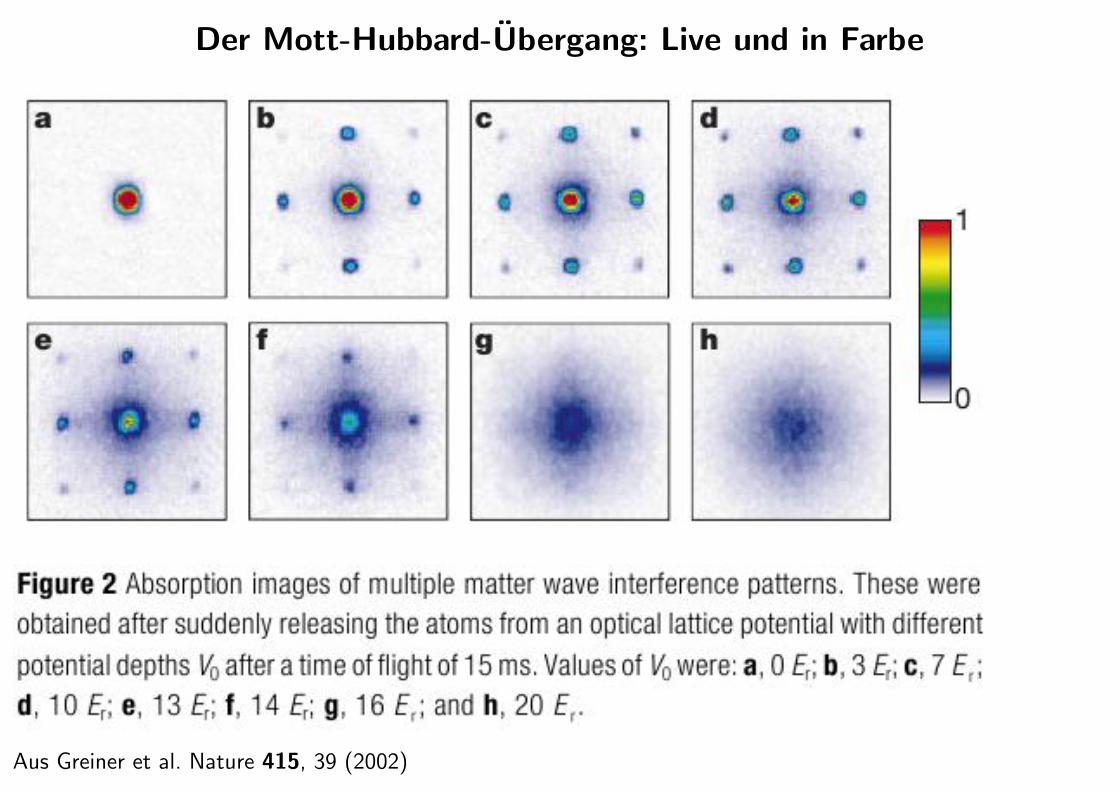
In the experiment of Greiner et al. [202] ultracoldbosonic 87Rb atoms were trapped in an optical lat-tice produced by a laser with lL = 852nm. The recoilenergy (11.8) then is ER ⇡ kB ·0.15µK and the trap-ping potential was V0 . 22ER. Non-interacting free(V0 = 0) bosons at zero temperature will condenseinto the lowest plane-wave state (11.3), with~k =~0.The situation does not change decisively if a weakinteratomic interaction and a weak lattice potentialare present: the state remains a macroscopically co-herent (superfluid) many-boson state.

With growing strength of the lattice potential V0, thesingle-particle states become progressively localizedand the repulsive interaction U dominates the Hamil-tonian (11.17) more and more. If the total number ofparticles is small enough, every lattice site (or po-tential well) contains at most one atom. For strongenough V0 each atom will be strongly localized inone potential well and will not enjoy enough overlap

to its neighbors to develop long-range phase coher-ence of the wave function. If every potential wellcontains exactly one atom2, further atoms can onlybe added at the price of an excitation energy U peratom. The same energy gap also prevents the for-mation of doubly occupied sites (and accompanyingvacancies) which would be needed to achieve par-ticle transport. The resulting state is obviously in-compressible and, thinking in terms of the original(electronic) Hubbard model, insulating. Therefore itis known as the Mott (-Hubbard) insulator state.

The transition between the superfluid and Mott in-sulating states was demonstrated in a time-of-flightexperiment [202]. For small or moderate potentialstrength V0 all bosons convene in the lowest-energyextended Bloch state in a coherent manner. As theBloch state is a periodically modulated plane wave(11.6) it contains Fourier components with different~g values, with ~g =~0 dominating as V0 goes to zero.In the experiment the optical potential is switchedoff suddenly and the atoms are allowed to expandfreely. The Fourier components with different~g sep-arate spatially according to their different propaga-tion speeds. After a fixed expansion time an absorp-tion image is taken. The absorption images of Figure11.17 therefore map directly the distribution of theatoms in reciprocal space.

For free atoms, (V0 = 0) the lowest-energy Blochstate is an unmodulated ~k = ~0 plane wave. Thecorresponding absorption image in Figure 11.17.atherefore shows a single spot in the center. As V0grows, additional Fourier components enter the low-est Bloch state and become visible in the absorptionimage, which develops into a two-dimensional pro-jection of the reciprocal lattice (Figure 11.17 b,c,andd). However, upon further growth of V0 the recipro-cal lattice spots fade away again, their intensity be-ing soaked up by a big central blob. That blob (Fig-ure 11.17 g and h) is witness to the fact that the statehas evolved into one where each potential minimumhouses one atom, with no phase relation betweenneighboring atoms and hence no interference visi-ble. The large extent of the central absorption spotin reciprocal space reflects the localization of each

2The situation is similar for any other integer number of atomsper site.

171


atom in real space. This shows clearly the change inthe nature of the ground state as the ratio U/t is var-ied. The expected change in the nature of the low-energy excitation spectrum from gapless in the su-perfluid state to gapped in the Mott insulating statecould also be observed [202] by analyzing tunnelingbetween neighboring potential wells which are ener-getically displaced with respect to each other in anapplied external field.

Figure 11.17: Absorption images reflecting theFourier component structure of themany-particle wave function of 87Rbatoms in an atomic lattice of strengthV0. Images were obtained afterswitching off the lattice potentialsuddenly and allowing atoms toexpand for 15 ms. Potential strengthsV0 in units of the recoil energy ER area:0, b:3, c:7, d:10, e:13, f:14, g:16,and h:20 [202].

Fermionic atoms in optical lattices have also beenstudied. Köhl et al. [225] stored a large number of40K atoms in a three-dimensional simple cubic lat-tice and obtained absorption images after switchingoff the potential and allowing the atoms to expandballistically. As the Pauli principle strictly forbidsdouble occupation of single-particle energy levels,the fermionic 40K atoms fill up the available Blochstates (11.6) up to the Fermi energy. The surfacein ~k space which separates occupied states (at lowenergy) from empty states (at high energy) is calledthe Fermi surface. For a simple cubic optical lat-tice potential of the form (11.2) the Fermi surface isspherical at low density, but less so at higher den-sity. For a completely filled band the Fermi surfaceis equal to the boundary of the first Brillouin zone.

The energy gap to the next higher band then is theminimum energy for a single-particle excitation. Forelectrons in a solid that situation corresponds to aninsulator (or a semiconductor, if the energy gap issmall enough). In contrast to the interaction-inducedMott insulator discussed above, the present case istermed band insulator and obviously does not rely oninteraction effects. In the optical-lattice experimenton 40K the shape of the Fermi surface could be mea-sured for various particle densities. Also, employingthe magnetic-field dependence of the scattering be-tween two spin species (Feshbach resonance), inter-action effects like the transfer of atoms into higherbands could be observed.

These pioneering experiments on bosonic andfermionic atoms in optical lattices show that quan-tum simulation of correlated many-body systemsmay soon be within reach of experimental possibil-ities. These exciting prospects have led to a verylarge number of proposals for correlation effects inmany-body systems that could be studied with atomsin optical lattices, see the review by Lewenstein et al.[218].

11.6.3 Universal optical lattice quantumcomputing?

The question mark in the title of this section impliesthe existence of problems impeding a straightfor-ward implementation of quantum information pro-cessing in optical lattice systems. The most impor-tant of these problems is the lack of addressabilityof individual qubits. While the simulation of corre-lated quantum many-body systems profits from thefact that all atoms in an optical lattice are equal andin essentially the same environment, universal quan-tum computing suffers from this indistinguishabilitysince the qubits cannot be addressed or manipulatedindividually, as necessary for running a non-trivialquantum algorithm.

To be able to distinguish between atoms the transla-tional symmetry of the optical lattice must be bro-ken. This can be achieved, for example, by apply-ing a magnetic field gradient which makes the transi-tion frequency of an atom depend on its position and

172


thus allows for different quantum operations at dif-ferent positions. A more radical approach would beto abandon the three-dimensional optical lattice withits µm-size lattice constant and replace it with a two-dimensional array of focused laser beams with a sin-gle atom trapped in each laser focus [198, 199]. Eachsuch focus is typically some µm in size and typicaldistances between neighboring foci are several tensof µm, so that individual atoms can be addressedwith an additional focused laser beam. The neces-sary arrays of microlenses can be manufactured bymicrooptical techniques.

Review: quantum simulations with ultracold atomicgases [226]

Problems

For sufficiently large potential strength V0 the opti-cal lattice potential (11.2) can be approximated by aharmonic oscillator potential

Vosc =mw

2

2~r2,

where~r is the D-dimensional vector of displacementfrom the potential minimum.

a) Calculate the Hubbard interaction U (11.15),approximating the Wannier function wn(~r) bythe normalized oscillator ground-state wavefunction

f0(~r) = p

�D/4a�D/2 exp�12

✓~ra

◆2

,

where a =q

hmw

is the characteristic length ofthe quantum harmonic oscillator. Show that Ugrows as V D/2

0 .

b) The nearest-neighbor hopping amplitude t canbe approximated by the overlap (the integralof the product of the wave functions) betweenthe ground-state wave functions in neighbor-ing potential wells. Calculate t and determineits dependence on the parameters of the opticallattice potential. Show that t decreases as V0grows.

173

11.5 Neutrale Atome und Quantencomputing/Quantensimulation

Gitter aus Licht

0

red detuningdipole in phase

blue detuningdipole out of phase

Eµe

E

E µe- . > 0E µe- . < 0

µe

Laser frequency

Force towards high field Force towards low field

Eine stehende Laserwelle (Spiegel...) mit Frequenz oberhalb oder unterhalb einer Resonanz sorgtdafur, dass das Induzierte Dipolmoment der Atome gegenphasig oder gleichphasig mit dem Feldschwingt. Das elektrische Dipolmoment ist also entweder antiparallel zum Feld, so dass dieDipole (Atome) vom starken Feld abgestoßen werden, oder parallel zum Feld, so dass sie zumstarken Feld hingezogen werden.

Gitter aus LinsenMit einer Matrix aus Mikrolinsen stellt man regelmaßig angeordnete Mikrobrennpunkte her, indenen sich Atome ansammeln.

(Bilder aus Dumke et al. Phys. Rev. Lett. 89, 097903 (2002))

Atome sortieren mit Forderbandern aus Licht

Langsame Phasenverschie-bung (kleine Frequenz-di↵erenz) zwischen dengegenlaufigen Strahlen bringtdie stehende Welle zumLaufen !

”Forderband“.

Zwei zueinander senkrech-te Forderbander konnen be-nutzt werden, um Atomeregelmaßig an gewunschtenStellen einzusortieren.(Miroshnychenko et al., Nature

442, 151 (2006); mit Videoclip)

11.6 Atome mit WW in optischen Gittern: Die etwas anderen Festkorper

Feynmans Idee: Simuliere ein Quantensystem durch ein anderes!

Manipulationen mit Licht

Aus Immanuel Bloch, Nature Physics 1,23 (2005).

Verschiedene Phasen im Lichtkristall

Links: Ortsraum; rechts: ImpulsraumAus Immanuel Bloch, Nature Physics 1,23 (2005).

Das Hubbard-Modell

Großenskalen:

”echter“ FK: a ⇠ 10

�10m, Elektron: punktformig.

”Lichtkristall“: a ⇠ �L ⇠ 10

�6m, Atom: r ⇠ aB ⇠ 10

�10m.

Potential des D-dimensionalen”Lichtkristalls“:

V (~r) = V0

DX

i=1

sin

2 kLri

Uberlagerung von D orthogonalen Laser-Stehwellen mit Wellenzahl kL = 2⇡/�L. PotentialstarkeV0 ⇠ Laserintensitat; schwach ~r-abhangig (Strahlprofil, Fokussierung)

Typische Energien

Wellenfunktion eines freien Teilchens:

~k(~r) =

1p⌦

ei~k·~r

(im Volumen ⌦). Energie:

"~k =

~2k2

2m.

Im Lichtgitter ist �L etwa gleich einer Resonanzwellenlange. Wird ein �L-Photon absorbiertoder emittiert, gibt es eine Ruckstoß-Energie

ER =

~2k2L

2m.

Das ist die typische Energieskala.

Periodisches Potential: ebene Wellen werden gitterpe-riodisch moduliert ! Blochfunktionen; Energiebanderweichen mehr oder weniger stark von Parabelform ab.Fur schwaches Potential V0 hat das niedrigste Band diemaximale Energie (Rand der Brillouinzone)

~2

2m

⇣⇡a

⌘2=

~2

2m

✓2⇡

�L

◆2

=

~2k2L

2m= ER. Bandstruktur fur starkes (links), schwa-

ches (Mitte) und verschwindendesLaser-PotentialAus I. Bloch, Nature Physics 1,23 (2005).

Hamiltonian nichtwechselwirkender Fermionen oder Bosonen in einem (z.B. optischen) Gitter

H =

X

~k,n

"~k,nc†~k,nc~k,n ,

n ist der Bandindex; die Erzeuger und Vernichter beziehen sich auf Blochfunktionen; statdessenkann man (besser fur unsere Diskussion) auch Wannierfunktionen nehmen.

wn(~r �~l) =

1pN

X

~k

e�i~k·~l n~k(~r).

~l ist der Gitterplatz, um den die Wannierfunktion zentriert ist. Fur große Gitterabstandegehen die Wannierfunktionen in atomare Wellenfunktionen uber. Hamiltonian, ausgedruckt imWannierbild:

H =

X

~l,~l0

t~l�~l0nc†~lnc~l0n ,

wo die Hopping-Elemente t~l�~l0n angeben, mit welcher Wahrscheinlichkeitsamplitude ein Platz-wechsel zwischen zwei Gitterplatzen stattfindet:

t~l�~l0n =

1

N

X

~k

"~knei~k·(~l�~l0).

Hopping-Elemente konnen auch als Uberlapp-Matrixelemente zwischen Wannierfunktionen anden beiden beteiligten Gitterplatzen geschrieben werden.

Fur starkes Potential V0: Wannierfunktionen stark in ihrer jeweiligen Potentialmulde lokalisiert,Uberlapp nur zwischen nachsten Nachbarn nennenswert! nur ein Hopping-Element �tn. Dannist die Bandstruktur

"~kn = �2tn

DX

i=1

cos kia.

~l ist der Gitterplatz, um den die Wannierfunktion zentriert ist. Fur große Gitterabstandegehen die Wannierfunktionen in atomare Wellenfunktionen uber. Hamiltonian, ausgedruckt imWannierbild:

H =

X

~l,~l0

t~l�~l0nc†~lnc~l0n ,

wo die Hopping-Elemente t~l�~l0n angeben, mit welcher Wahrscheinlichkeitsamplitude ein Platz-wechsel zwischen zwei Gitterplatzen stattfindet:

t~l�~l0n =

1

N

X

~k

"~knei~k·(~l�~l0).

Hopping-Elemente konnen auch als Uberlapp-Matrixelemente zwischen Wannierfunktionen anden beiden beteiligten Gitterplatzen geschrieben werden.

Fur starkes Potential V0: Wannierfunktionen stark in ihrer jeweiligen Potentialmulde lokalisiert,Uberlapp nur zwischen nachsten Nachbarn nennenswert! nur ein Hopping-Element �tn. Dannist die Bandstruktur

"~kn = �2tn

DX

i=1

cos kia.

Und jetzt mit Wechselwirkung!

Welche Wechselwirkung? Wegen der Großenverhaltnisse ist nur langreichweitiger Anteil interes-sant; parametrisierbar durch Streulange aS:

Vint(~r � ~r0) =

4⇡~2

maS�(~r � ~r0

).

Gestalt des Wechselwirkungs-Hamiltonians in Wannierdarstellung: Summe von Termen mitjeweils• zwei Erzeugern und zwei Vernichtern• einem Integral (Matrixelement) aus 4 Wannierfunktionen an 4 (oder weniger) Gitterplatzenund dem Wechselwirkungspotential.

Wegen starker Lokalisierung durch starkes Potential dominiert der Term, bei dem alle vierWannierfunktionen an einem Platz sitzen. Die Wechselwirkung ist dann gegeben durch dieEnergie

U =

4⇡~2

maS

Zd3r |wn(~r)|4.

Wenn alles sich in einem Band abspielt, lassen wir den Bandindex n weg und erhalten furSpin-1/2-Fermionen das Hubbard-Modell:

H = �tX

~l,~l0,�

c†~l�c~l0� + UX

~l

n~l"n~l#

(~l,~l0 nachste Nachbarn), n~l� := c†~l�c~l� ist der Teilchenzahloperator. Das Pauliprinzip diktierthier die Spin-Kombination im Wechselwirkungsterm: gleicher Spin ist verboten.

Bosonen mogen gleichen Spinzustand, und fur Bosonen im gleichen Spinzustand ist das”Bose-

Hubbard-Modell“

H = �tX

~l,~l0

c†~l c~l0 +U

2

X

~l

n~l(n~l � 1).

Wenn alles sich in einem Band abspielt, lassen wir den Bandindex n weg und erhalten furSpin-1/2-Fermionen das Hubbard-Modell:

H = �tX

~l,~l0,�


~l

n~l"n~l#

(~l,~l0 nachste Nachbarn), n~l� := c†~l�c~l� ist der Teilchenzahloperator. Das Pauliprinzip diktierthier die Spin-Kombination im Wechselwirkungsterm: gleicher Spin ist verboten.

Bosonen mogen gleichen Spinzustand, und fur Bosonen im gleichen Spinzustand ist das”Bose-

Hubbard-Modell“

H = �tX

~l,~l0

c†~l c~l0 +U

2

X

~l

n~l(n~l � 1).

Der Steuerparameter des Hubbardmodells ist das Verhaltnis t/U , und das kann mit dem Lasereingestellt werden:

U ⇠ VD4

0 t ⇠ e�constpV0

Grenzfalle des Grundzustands sind gut verstanden.

Vom k-Raum zum Ortsraum: Einfach abwarten...

87Rb

Aus Greiner et al. Nature 415, 39 (2002)

Der Mott-Hubbard-Ubergang: Live und in Farbe


Kollaps und Wiederbelebung


Plotzliches Umschalten von t/U macht aus einem Eigenzustand des Hamiltonians eine Super-position, die Oszillationen zeigt.

Fermisystem ohne Wechselwirkung : Fermiflache

Aus Immanuel Bloch, Nature Physics 1,23 (2005).

Fermisystem mit Wechselwirkung

Sauberer Festkorper ohne Fehlstellen, Gitterschwingungen...; mit kontrollierbaren Parametern:

2 · 10

5 40K-Atome in den Gesamtspinzustanden |F,mF i = |92,�92i = | #i und |92,�

72i = | "i ...

...in einem (Licht-) Potential aus zwei unabhangigen Komponenten: periodisch + parabolisch.

Parabolisches Potential druckt die Fermionen im (festen) Gitter zusammen; im realen Festkorperwird das Gitter bei Kompressibilitatsmessungen dagegen immer mit komprimiert.

Hubbardmodell:

H = �tX

~l,~l0,�


~l

n~l"n~l# +

X

~l

VParabel(~l)(n~l" + n~l#)

Das Hubbard-U kann uber eine Feshbach-Resonanz gesteuert werden (Streulange; vgl. Duineund Stoof, Physics Reports 396, 115 (2004)).

Achtung: t heißt bei den Atomphysikern immer J .

Sauberer Festkorper ohne Fehlstellen, Gitterschwingungen...; mit kontrollierbaren Parametern:

2 · 10

5 40K-Atome in den Gesamtspinzustanden |F,mF i = |92,�92i = | #i und |92,�

72i = | "i ...

...in einem (Licht-) Potential aus zwei unabhangigen Komponenten: periodisch + parabolisch.

Parabolisches Potential druckt die Fermionen im (festen) Gitter zusammen; im realen Festkorperwird das Gitter bei Kompressibilitatsmessungen dagegen immer mit komprimiert.

Hubbardmodell:

H = �tX

~l,~l0,�


~l

n~l"n~l# +

X

~l

VParabel(~l)(n~l" + n~l#)

Das Hubbard-U kann uber eine Feshbach-Resonanz gesteuert werden (Streulange; vgl. Duineund Stoof, Physics Reports 396, 115 (2004)).

Achtung: t heißt bei den Atomphysikern immer J .

Was erwartet man?

Isolator-Phasensind inkompressibel:Doppelbesetzungoder Transfer inhoheres Energie-band sind teuer.

Große der Atomwolke in Abhangigkeit von der Kompressionsstarke, fur verschiedene Werte derHubbard-Abstoßung U .Bilder zeigen die Fermiflache (fur U = 0); bei E ist das Band voll; weitere Kompressionunmoglich.

Rechte Seite:”Hochzeitstor-

ten“-Struktur der Dichte, mitPlateaus bei einem (Mott-Isolator) bzw zwei (alles voll)Teilchen pro Gitterplatz.(Beachte: Hier ist die Zahl derTeilchen pro Platz und Spin-richtung aufgetragen ! Fak-tor 2.)

Kompressibilitat in Abhangigkeit von der Kompressionsstarke, fur verschiedene Werte derHubbard-Abstoßung U . Das Minimum in der Kurve C ist die Signatur des Mott-Isolators (1Fermion pro Gitterplatz).

Noch ein Trick: Kunstliche Magnetfelder

Neutrale Atome konnen an reale Magnetfelder hochstens schwach uber ihre Dipolmomentekoppeln ! Studium der E↵ekte von Magnetfeldern auf geladene Teilchen (Quanten-Hall-E↵ekt...) ist in diesen Modellsystemen nicht moglich.



Oder vielleicht doch?




Wie wirkt ein Magnetfeld auf ein geladenes Teilchen?

~p �! ~p� q ~A(~r)

bewirkt eine zusatzliche ortsabhangige Phasenverschiebung in der Wellenfunktion.

Noch ein Trick: Kunstliche MagnetfelderNeutrale Atome konnen an reale Magnetfelder hochstens schwach uber ihre Dipolmomentekoppeln ! Studium der E↵ekte von Magnetfeldern auf geladene Teilchen (Quanten-Hall-E↵ekt...) ist in diesen Modellsystemen nicht moglich.


Wie wirkt ein Magnetfeld auf ein geladenes Teilchen?

~p �! ~p� q ~A(~r)

bewirkt eine zusatzliche ortsabhangige Phasenverschiebung in der Wellenfunktion.

Versuche eine derartige Phasenverschiebung auf optischem Weg zu erreichen.

Bose-Einstein-Kondensat aus bis zu 2.5 ·10

5 87Rb-Atomen.Der Grundzustand hat Gesamtspin F = 1.mF = 0,±1 spalten in einem Magnetfeld auf. Die Atome bewegen sich gemaß der Dispersions-relation

E(

~k,mF ) =

~2k2

2m+ ~!ZmF

(!Z = Zeeman-Aufspaltung).

Raman-Prozess koppelt die verschiedenen mF -Komponenten anein-ander: Emission und Absorption von zwei Photonen mit passenderDi↵erenzfrequenz, nahe dem Ubergang zu einem angeregten Hilfszustand.

Trick: Verwende zwei Raman-Laser unterschiedlicher Strahlrichtung! mF -abhangiger Impulsubertrag auf das Atom.

(Aus Lin et al. Phys. Rev. Lett. 102, 130401 (2009))

|0>

|1>

|aux>

bla

Oberes Bild:Die Parabel-Dispersionen der Atome mit unter-schiedlichem mF sind gegeneinander verschoben(dunne schwarze Linien). Der Raman-Prozess kop-pelt die Zustande mit einer Starke (Rabifrequenz)⌦R. In der Rotating-Wave-Approximation hat dieHamiltonmatrix fur den relevanten Unterraum dieGestalt:

(�: Verstimmung der Ramanlaser-Frequenz-di↵erenz gegenuber !Z, ✏ ist die Zeeman-Verschiebung 2. Ordnung fur mF = 0.) DieEigenwerte sind die dicken roten Linien, fur� = 0. Das Minimum liegt bei k = 0.

Unteres Bild:Wie oben, aber � 6= 0; das Minimum liegt beieinem endlichen k:

E(k)� E0 ⇡1

2m(~(k � k0))

2=

1

2m(p� q ˜A)

2

Das synthetische Vektorpotential ˜A hangt von der Verstimmung � ab, die uber das (reale) Ma-gnetfeld ortsabhangig gemacht werden kann ! synthetisches Magnetfeld.

Das Bose-Einstein-Kondensat besitzt eine gemeinsame makroskopi-sche Wellenfunktion ! Flussquantisierung des (synth.) Magnetfelds,ahnlich wie beim Supraleiter. Flussquanten außern sich als Wirbellinien(vortices).Diese wurden (mit einer etwas anderen Geometrie als oben beschrie-ben) von Lin et al. (Nature 462, 628 (2009)) beobachtet.

B=0/ B=0

Supraleiter

Loch

Einige experimentelle Details:

11 Trapped Ions and Atoms - TU Dortmund

Documents

Transcript of 11 Trapped Ions and Atoms - TU Dortmund