Modeling the Whole Firm:

The Effect of Multiple Inputs

and Financial Intermediation on Bank Deposit Rates

Elizabeth K. Kiser∗

June 3, 2003

Abstract

Empirical studies of price competition typically analyze the direct effects of marketstructure, cost, and local demand on prices; this approach has been applied widely tostudies of bank deposit rates. However, the theory of the banking firm suggests thatsubstitutability between sources of deposits and conditions in the bank loan marketshould also affect the pricing of retail deposits. This paper develops a theoretical modelto incorporate these effects, and tests the predictions empirically using institution-leveldeposit rate data from Bank Rate Monitor. The results suggest that the cost of large-scale deposits affects how banks price retail deposits, and that conditions in lendingmarkets feed back into retail deposit rates.

JEL Codes:L0–Industrial Organization: GeneralG2–Financial Institutions and Services

∗Economist, Federal Reserve Board, 20th and C St., NW, Washington, DC 20551,elizabeth.k.kiser@frb.gov. The views expressed herein are those of the author and not nec-essarily those of the Federal Reserve Board. Bob Adams, Dean Amel, Allen Berger, RonBorzekowski, Ken Brevoort, Diana Hancock, Erik Heitfield, Robin Prager, Alicia Robb,Paul Smith and Christina Wang provided helpful comments. Eli Mou provided researchassistance.

1 Introduction

Industrial organization research has paid considerable attention to the effects of market

structure, cost, and local demand on pricing. This approach has generally been followed in

studies of bank deposit rates. However, for firms with market power, conditions in input and

output markets can feed back to affect pricing of both inputs and outputs, and a firm’s input

mix decision can affect the pricing of the respective inputs. In the case of banking, the theory

of the bank as an intermediary – a matchmaker of lenders with borrowers – suggests several

such factors that may affect retail deposit rates. First, bank loan and deposit rates may be

jointly determined, implying that conditions in loan (output) markets feed back to deposit

(input) markets. Second, substitutability among inputs in the production of loans suggests

that the prices of different deposit types will affect one another. In particular, a bank’s

cost of large-scale deposits, for which the bank is a price taker, can affect its pricing of retail

deposits, over which it has some market power. These factors have been largely overlooked in

the literature on competition for bank deposits. This paper provides a theoretical framework

of how intermediation and the input mix decision impact pricing, and tests these predictions

empirically.

The model presented here expands on earlier classical models of the banking firm by

incorporating factors that affect equilibrium values by shifting retail deposit supply, loan de-

mand and cost, the cost of managing retail deposits, and the cost of attracting and managing

wholesale deposits. Comparative static results are tested using a unique data set of directly

measured interest rates for four retail deposit products offered by banks and thrifts, linked

to data on institution and market characteristics. The directly measured rates are a sub-

stantial improvement over commonly used price measures that are computed from balance

sheet variables and contain considerable measurement error.

The empirical results show that both bank risk, which affects its cost of wholesale funds,

1

and local lending conditions, which influence the pricing of its output, appear to affect retail

deposit rates. The findings are consistent with the model’s prediction that an institution’s

lower cost of wholesale funds results in its offering lower retail deposit rates, and that con-

ditions in loan markets can feed back into deposit pricing. These results suggest that the

deposit and loan (i.e., the input and output) pricing decisions are not likely separable for

most banks. An important implication is that banks are likely to pass through changes in

federal funds rates to lending markets – the so-called bank lending channel for monetary

policy. The data also indicate that banks with local market power are likely to pay lower de-

posit rates, confirming the importance of local competitive conditions. Finally, a differential

relationship is found between some variables and rates for liquid and time deposits, which

implies either that banks do not perceive these products to be perfect substitutes as inputs

in the production of loans, or that depositors do not perceive liquid and time deposits to be

close substitutes.

1.1 The Banking Firm

Banks offer an expanding range of products and services. Nevertheless, banks continue

to serve an intermediary function by borrowing funds from depositors and using these to

fund lending activities.1 As of 2001, total interest income comprised 72 percent of total

income for commercial banks in the U.S.2, and depository institutions remain the most

important source of financing for consumers and small businesses. The process of financial

intermediation has received considerable attention in the literature. Traditional theoretical

1The question has arisen whether deposits should be categorized as inputs or outputs. Hancock (1985)uses the net costs of financial firms’ assets and liabilities to determine inputs and outputs. She notes thatfluctuations in interest rates and other variables can result in deposits being categorized as either inputs oroutputs. In contrast, Sealey and Lindley use the terminology of Frisch (1965), calling deposits a “limitationalinput” - one whose increase in usage “is a necessary, but not sufficient, condition for an increase in output.”(See also Berger and Humphrey (1992).) The analysis here relies on this theoretical notion and designatesdeposits as inputs.

2Source: Federal Deposit Insurance Corporation (FDIC).

2

models of the banking firm include Tobin (1958), Klein (1971), Monti (1972), and Sealey

and Lindley (1977); surveys of this literature are provided in Santomero (1984) and Freixas

and Rochet (1997). In these models, the bank is assumed to face an upward-sloping supply

of core (retail) deposits and operate as a price taker in a larger-scale funds market (such

as federal funds). The bank finances initial loans using less costly core deposits, bidding

up the core deposit rate to the point where the marginal cost of core deposits equals the

federal funds rate. At this point the bank switches over to federal funds to finance loans

at the margin. This model implies that for sufficiently high loan demand relative to core

deposit supply, a bank’s marginal loan quantity and price may be chosen separately from

the quantity and price of core deposits.

Following up on these earlier models, several papers consider the role of funding sources

in the “bank lending channel” of monetary policy; see Kashyap and Stein (2000) for a

brief review of this literature. The bank lending channel refers to the mechanism by which

banks pass through changes in the federal funds rate to the rates they charge on loans.

The existence of a bank lending channel relies on the premise that banks have no (major)

source of funding other than core deposits and federal funds. If banks use federal funds

to fund marginal loans, then the federal funds rate will affect the loan rates banks charge.

However, if banks have access to outside funding sources that are less costly than federal

funds, banks may be able to make lending decisions that are unaffected by the federal funds

rate, and that are separable from retail deposit-taking. Thus, if independence holds between

the pricing of core deposits and loans, it follows that the federal funds rate is irrelevant to

bank lending decisions, and no bank lending channel for monetary policy exists. In a recent

paper, Jayaratne and Morgan (2000) find evidence that limited access to uninsured funds

constrains small bank origination of loans, providing evidence in support of a bank lending

channel for these institutions, with greater independence between lending and deposit taking

(and less of a bank lending channel) for large institutions.

3

An extensive body of literature exists on competition in retail deposits, largely distinct

from the work on financial intermediation. Much of the work in this area has focused on the

relationship between concentration and profits or prices (for example, Berger and Hannan

(1989)). Other papers address questions of market definition (Amel and Hannan (1999),

Amel and Starr-McCluer (2002) and Heitfield (1999)) and the price effects of mergers (Prager

and Hannan 1998); two other papers take a structural approach to evaluating market power

(Adams, Roller and Sickles (2002) and Dick (2002)). With the exception of Adams et al.

all these papers generally assume independence between deposit taking and lending and do

not treat retail deposits as an input in the production of loans. Adams et al. consider the

joint decision between deposit and loan rate setting, but perform their analysis at a highly

aggregated level. The analysis presented here uses firm-level data to investigate issues raised

in both the lending-channel papers and the competition work, and suggests that future work

on competition for retail deposits should incorporate alternative sources of funding as well

as the effect of lending on retail deposit rates.

1.2 Retail and Wholesale Deposits

This study considers the effect of bank access to large-scale, or “wholesale,” deposits on retail

deposit rates. Banks may differ in their rates paid to obtain wholesale deposits or in their

cost of managing wholesale funds. In particular, well capitalized banks with less risky asset

portfolios (or banks that are considered “too big to fail”) may pay a lower risk premium for

wholesale funds than their riskier counterparts. Similarly, larger banks may experience scale

economies in managing wholesale deposits and may receive quantity discounts (i.e., lower

rates on larger loan volumes), making wholesale funds less costly. If wholesale funds are used

as substitutes for retail deposits in funding loans, and if the bank faces an upward-sloping

supply of retail deposits, then its ability to buy wholesale funds at low cost should reduce

4

its demand for retail deposits, as it can buy cheap wholesale funds and avoid bidding up

the price of the alternative input. This effect, distinct from competitive conditions in local

deposit markets, could be increasingly important in explaining how prices are set for retail

deposits, as consolidation has resulted in larger, more diversified banks.

The “retail” and “wholesale” categories in the model below are based on the nature of

deposit supply.3 First, retail and wholesale funds constitute distinct product markets based

on depositor substitution patterns and depositor risk. Retail products such as checking and

savings accounts and small-denomination certificates of deposit (CDs) are insured by the

FDIC and are typically held by individuals or small firms. In contrast, instruments such as

large-denomination CDs (those in denominations greater than $100,000) and subordinated

debt are uninsured and tend to be held by larger-scale institutional investors and wealthy

individuals. The suppliers of each type of deposit therefore appear to represent distinct sets

of customers as well as different degrees of depositor risk.4

Second, banks face differing elasticities of supply in retail versus wholesale deposits. Con-

ditional on risk, wholesale funds are homogeneous and exchangeable over a broad (national

or international) geographic area, and no single firm holds a substantial market share. In

contrast, a depository institution may command some degree of market power (ability to

affect prices unilaterally) in retail deposits, arising from several factors. Retail customers’

documented use of local depository institutions suggests that firms with large local market

shares may hold market power in a local area.5 Furthermore, if customer switching costs

are present, then even a small institution may hold some market power over its own retail

3Note that the terms “retail” and “wholesale” in this context do not refer to a vertical sales structure,but rather to two separate deposit markets.

4A formal test whether retail and wholesale deposits constitute separate product markets would includeestimation of cross-elasticities of supply; no data are currently available to perform such estimation.

5Amel and Starr-McCluer (2002) use data from the 1998 Survey of Consumer Finances to document thedistance between households and their depository institutions. They report that the median distance froma household to its main depository institution has been fairly stable over a 10-year period at 3 miles.

5

deposit customers.6 Finally, differentiation in non-price factors across banking institutions,

such as the size and location of ATM or branch networks, may allow some institutions to

hold greater market power than if deposit relationships were homogeneous.7

Note that although the federal funds rate, referenced in the earlier models, is absent

from the model presented below, the reader can consider federal funds to constitute a single

component of the broader category of wholesale funds. Note that while the Federal Open

Market Committee sets a target for the federal funds rate, the rates paid on individual federal

funds transactions between banks vary substantially and depend generally on institution

risk.8 Hence, rather than considering federal funds to constitute a fixed-rate market at

which all institutions can borrow, it should be considered one of several types of large-scale

funds which may be substituted for retail deposits.

Interactions between markets for retail and wholesale deposits may be increasing in im-

portance over time as consolidation occurs. Figure 1 shows the ratio of total insured deposits

to total liabilities over the period 1992-2001 for banks and thrifts. Over this period the ratio

of insured deposits to liabilities dropped from 56 to 40 percent for banks and from 78 to 50

percent for thrifts. This decline was a result of two simultaneous trends: a decline in the

ratio of insured to uninsured deposits along with a decline in total deposits as a proportion

of total liabilities.9 Note that these trends occurred simultaneously with industry consolida-

tion; figure 2 shows that the number of banks fell from 11,462 to 8080 over the period, while

the number of thrifts fell from 2390 to 1533. As banks and thrifts have consolidated, they

6For a survey of the theoretical implications of switching costs, see Klemperer (1995). Kiser (2002) givesempirical results from a survey on household switching behavior at depository institutions. About a third ofcustomers report that a main reason they have maintained their relationship with their depository institutionis that it would be too inconvenient to change banks.

7Eaton and Lipsey (1996) provide a broad survey of the economics of product differentiation. For amore specialized model of the effect of ATM networks on the pricing of deposit services, see Massoud andBernhardt (2002).

8Furfine (2001) provides an excellent summary of the economics of individual federal funds transactions.9Among nondeposit liabilities, “other borrowed funds” experienced the strongest increase in portfolio

share.

6

appear to rely less heavily on core deposits and draw more funds from larger markets.

2 The Theoretical Model

2.1 Setup

The model developed here is constructed to illustrate the effect of both the input mix decision

and intermediation on retail rates. The model is based loosely on the classical models of

Klein and Monti, and expanded to incorporate flexible functional forms for deposit supply

and loan demand and to introduce shift parameters that affect cost and demand. New

comparative statics and welfare effects are then derived to evaluate the impact of changes in

model parameters and to make predictions for empirical work.

The model is based on three key assumptions: (1) at low levels of total deposits, banks

find retail deposits less costly to obtain and manage than wholesale deposits, (2) banks hold

market power in retail deposits and lending but no market power in wholesale deposits, and

(3) the retail deposit supply, wholesale deposit supply, and loan demand functions faced by

a bank are entirely distinct.

The bank is assumed to take deposits and extend loans. Retail and wholesale deposits

are available to the bank as perfectly substitutable inputs in the production of loans. Fee

income and revenue from investment activities other than lending are excluded, and no

reserve requirement appears in the model. The primary results are not dependent on these

assumptions. The exposition describes a monopoly bank; however, this type of model can be

extended to a case of imperfect competition which gives similar comparative static results.10

The bank produces loans according to a linear production function, where the quantity

of loans L produced is less than or equal to the sum of retail deposits DR and wholesale

10See Freixas and Rochet (1997) p. 60.

7

deposits DW taken:

L(DR, DW ) ≤ DR + DW . (1)

The bank faces an inverse demand for loans rL(L), an inverse supply of retail deposits

rR(DR), and a perfectly elastic supply of wholesale deposits DW at rate rW . Assume a stan-

dard, upward-sloping retail deposit supply function that satisfies the following conditions:

r′R > 0 ∀DR > 0,

r′R(0) < ∞,

2 r′R + DR r′′R ≥ 0 ∀DR > 0. (2)

Assume a standard downward-sloping loan demand function, with:

r′L < 0 ∀L > 0,

r′L(0) > −∞,

2 r′L + L r′′L ≤ 0 ∀L > 0. (3)

These functional forms are more general than the linear case presented in the Klein and

Monti models. Weak convexity of retail deposit supply is sufficient but not necessary to

satisfy the final condition in (2); this assumption is standard in Cournot models and is not

restrictive. Similarly, the final expression in (3) is a less restrictive condition than weak

concavity.

Let rR(0) designate the retail rate that induces the first unit of retail deposits to be

supplied. Assume that this value is less than the wholesale rate:

rR(0) < rW . (4)

8

The monotonicity of retail deposit supply along with (4) implies that for the first unit

of loans, the marginal cost to the bank of retail deposits is less than the marginal cost of

wholesale funds. The assumptions in (4) and (2) imply that the bank’s marginal cost curves

for retail and wholesale deposits intersect.

Define DR as the level of retail deposits such that the marginal cost of retail deposits

equals the marginal cost of wholesale deposits; that is, DR satisfies

rR(DR) + DR r′R(DR) = rW . (5)

The assumptions in (2) and (4) imply that DR is nonnegative. The bank’s cost-minimization

problem results in the following cost function:

C(rR, rW , L) =

rR(L)L if L ≤ DR,

rR(DR)DR + rW [L− DR] otherwise.(6)

2.2 Profit Maximization

The bank’s profit equals loan revenue minus deposit interest. The firm’s profit-maximization

problem is

maxL

Π(L) =

[rL(L)− rR(L)]L if L ≤ DR,

rL(L)L− rR(DR)DR − rW [L− DR] otherwise.(7)

Because the bank’s marginal cost of deposits is continuous and weakly increasing and its

marginal loan revenue is continuous and strictly decreasing, a unique maximum exists. Define

L∗ = arg maxL

Π(L). (8)

For total lending levels below DR, profit maximization reduces to simple monopoly quantity

9

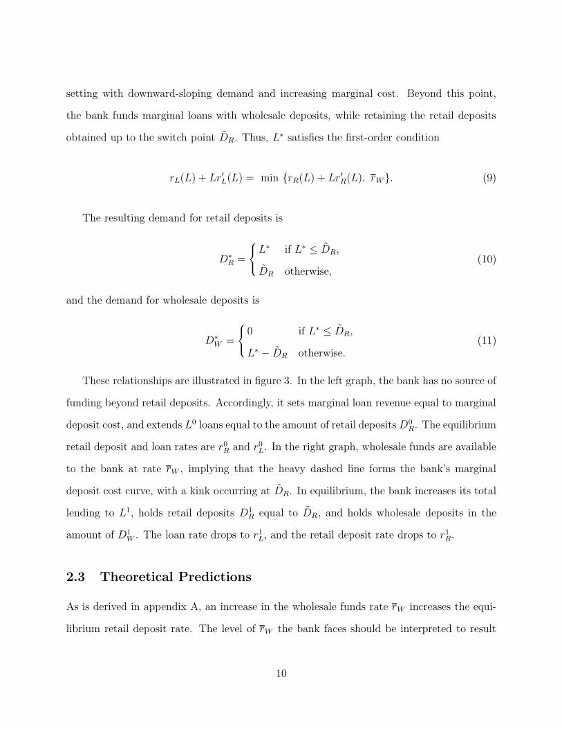
setting with downward-sloping demand and increasing marginal cost. Beyond this point,

the bank funds marginal loans with wholesale deposits, while retaining the retail deposits

obtained up to the switch point DR. Thus, L∗ satisfies the first-order condition

rL(L) + Lr′L(L) = min {rR(L) + Lr′R(L), rW}. (9)

The resulting demand for retail deposits is

D∗

R =

L∗ if L∗ ≤ DR,

DR otherwise,(10)

and the demand for wholesale deposits is

D∗

W =

0 if L∗ ≤ DR,

L∗ − DR otherwise.(11)

These relationships are illustrated in figure 3. In the left graph, the bank has no source of

funding beyond retail deposits. Accordingly, it sets marginal loan revenue equal to marginal

deposit cost, and extends L0 loans equal to the amount of retail deposits D0R. The equilibrium

retail deposit and loan rates are r0R and r0

L. In the right graph, wholesale funds are available

to the bank at rate rW , implying that the heavy dashed line forms the bank’s marginal

deposit cost curve, with a kink occurring at DR. In equilibrium, the bank increases its total

lending to L1, holds retail deposits D1R equal to DR, and holds wholesale deposits in the

amount of D1W . The loan rate drops to r1

L, and the retail deposit rate drops to r1R.

2.3 Theoretical Predictions

As is derived in appendix A, an increase in the wholesale funds rate rW increases the equi-

librium retail deposit rate. The level of rW the bank faces should be interpreted to result

10

from a bank’s portfolio risk. While the theoretical model takes rW to be exogenous, the

empirical model presumes that heterogeneity in risk across banks results in differing rates

paid for large-denomination funds.

In addition to the wholesale rate, other factors that shift demand, cost and risk may

also affect retail rates. These factors, which were absent in the Klein-Monti models, can be

incorporated in a straightforward way. Comparative static results for retail deposit operating

cost θR, wholesale deposit operating cost θW , loan operating cost θL, retail deposit supply σR,

and loan demand σL are derived in appendix A and summarized in table 1. Most predicted

signs depend on the range of output, according to whether L∗ exceeds DR (whether wholesale

funds are employed).

Most of the expected signs are straightforward; a few are initially counterintuitive. Note

that for a level of retail deposits below the switch point DR, an increase in retail deposit

operating cost increases the total marginal cost of deposit taking by the bank, thereby

decreasing the optimal level of lending and deposit taking. Because retail deposit supply

slopes upward, this results in a decrease in the equilibrium retail deposit rate. Similarly,

an increase in loan operating cost results in a decrease in the optimal level of lending and

deposit taking, and in turn a decrease in the retail deposit rate paid.

The model is constructed to illustrate the effects of the input mix decision and inter-

mediation on retail rates. The model could be extended easily to allow for an increasing

marginal cost of wholesale funds (or multiple types of substitutable funds). In this case,

the bank would equilibrate the marginal cost of each deposit type to marginal loan revenue.

Assuming that the marginal cost of each deposit type is increasing, and if the rates required

to attract the first dollar of each deposit type are similar, it would be profitable to use a

single deposit type only at low levels of lending. Once rates are bid up to attract the initial

dollar of each deposit type, it would never be profitable to use only one deposit type at

the margin. Substitution among deposit types would be continuous rather than discrete,

11

and no switchover point analogous to DR would exist. Consequently, the (nonzero) signs of

the derivatives shown in table 1 would apply regardless of whether the bank is employing

wholesale funds.

2.4 Welfare Effects

The comparative statics show that a lower cost of wholesale funds results in greater total

lending and lower loan rates. It follows that a lower rW should increase borrower welfare.

However, decreasing rW also decreases both retail deposits and the rate paid to retail depos-

itors. The effect of the cost of wholesale funds on borrower, depositor and bank surplus and

the net effect on total welfare is calculated in appendix B. Note that because the wholesale

rate rW is assumed to be determined in a perfectly competitive market, zero economic profits

accrue to wholesale depositors. Also, because the wholesale funds rate has no effect when

the bank does not find it profitable to use wholesale funds, only the case where D∗

W > 0 is

considered.

The derivation shows that the effect on total surplus of the wholesale funds rate depends

on the relative curvature and magnitudes of retail deposit supply and loan demand. Sym-

metric curvature of retail deposit supply and loan demand results in the gains to borrowers

from a drop in rW exceeding the corresponding loss to retail depositors. (This result is driven

by the assumption that wholesale depositors receive zero surplus.) This observation is im-

portant from a policy perspective; while we might infer that less competitive retail deposit

rates are a negative outcome of an increase in institution size, this loss in consumer surplus

may be more than offset by lower loan rates, all else equal. This assumes, of course, that

the competitive environment is held constant. Aside from the model, increasing firm size

through consolidation could also result in greater market power in both loans and deposits,

so that the increase in consumer surplus from cheaper wholesale funds could in turn be offset

12

by increased rates due to greater market power.

3 Empirical Estimation

The empirical model differs from the theoretical model in a few ways. Most notably, the

markets for retail deposits and loans are assumed in the theoretical model to be monopoly

markets; no strategic interaction occurs among firms. Recall that the model can be extended

to incorporate imperfect competition among several firms.

While the theoretical model examines the decision of a single bank facing a single whole-

sale funds rate, banks in the population vary in the rates they must pay for wholesale funds

(as well as along other dimensions). The empirical analysis is conducted under the assump-

tion that each bank is a price taker in wholesale deposits, and that levels of rW vary across

the population of banks. The process generating these differences in wholesale rates is not

modeled here; however, the empirical models are based on the premise that wholesale rate

or cost differences may result from differences in bank risk, scale, or differences in cost or

demand.

Equation (9) can be solved implicitly for r∗R as

r∗R = f(rW , θW , θR, σR, σL, θL). (12)

Two model specifications are estimated, both as linearized versions of this reduced form.

The first model specification is run in an OLS framework:

rpim = βp ′ Xim + εp

im, (13)

where p ∈ {1, ..., 4} indexes four specific retail deposit products (interest checking accounts,

MMDAs, and 6- and 12-month CDs), i indexes institutions, and m indexes markets. Xim is

13

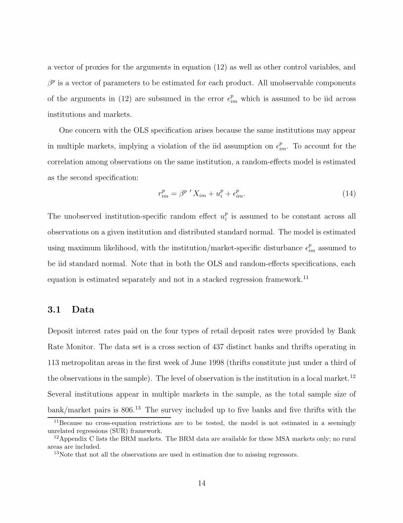
a vector of proxies for the arguments in equation (12) as well as other control variables, and

βp is a vector of parameters to be estimated for each product. All unobservable components

of the arguments in (12) are subsumed in the error εpim which is assumed to be iid across

institutions and markets.

One concern with the OLS specification arises because the same institutions may appear

in multiple markets, implying a violation of the iid assumption on εpim. To account for the

correlation among observations on the same institution, a random-effects model is estimated

as the second specification:

rpim = βp ′ Xim + up

i + εpim. (14)

The unobserved institution-specific random effect upi is assumed to be constant across all

observations on a given institution and distributed standard normal. The model is estimated

using maximum likelihood, with the institution/market-specific disturbance εpim assumed to

be iid standard normal. Note that in both the OLS and random-effects specifications, each

equation is estimated separately and not in a stacked regression framework.11

3.1 Data

Deposit interest rates paid on the four types of retail deposit rates were provided by Bank

Rate Monitor. The data set is a cross section of 437 distinct banks and thrifts operating in

113 metropolitan areas in the first week of June 1998 (thrifts constitute just under a third of

the observations in the sample). The level of observation is the institution in a local market.12

Several institutions appear in multiple markets in the sample, as the total sample size of

bank/market pairs is 806.13 The survey included up to five banks and five thrifts with the

11Because no cross-equation restrictions are to be tested, the model is not estimated in a seeminglyunrelated regressions (SUR) framework.

12Appendix C lists the BRM markets. The BRM data are available for these MSA markets only; no ruralareas are included.

13Note that not all the observations are used in estimation due to missing regressors.

14

largest deposit market shares in each market; the median assets across institution/market

observations in the sample is $7.8 billion.14 While the sample slightly overrepresents thrift

institutions, it does generally represent the largest-share institutions operating in the largest

metropolitan areas. Because of the emphasis on larger institutions, this sample is arguably

more appropriate than a representative sample of U.S. depository institutions for examining

the effects of wholesale funds markets on retail prices, as one would expect larger institutions

to be more likely than smaller institutions to participate heavily in markets for wholesale

funds.

In addition to the stratification scheme, the Bank Rate Monitor data are particularly

useful for this application because they are directly measured and available for multiple

products. Directly measured retail deposit rates are often difficult to obtain. The rates used

in many studies are computed from institution income statements and balance sheets and

are available only at the institution and not the market level, which presents a problem in

the case of multi-market institutions. In addition, comparable numbers for specific deposit

products are generally not available for both banks and thrifts. Aggregating over markets

and deposit products to construct prices can result in considerable measurement error. In

addition, the availability in this sample of several types of deposit rates means that separate

estimates can be obtained for products for which consumer demand, firm cost, or competition

may vary. Furthermore, the results from estimation using multiple products can be compared

to determine whether patterns are spurious or systematic.

Many variables from other sources are linked to the Bank Rate Monitor data. How these

variables serve as proxies for components of the profit function is described below. Means

and standard deviations of variables are presented in table 2.

14Some markets contained fewer than five institutions of each type, so some markets total fewer than teninstitutions.

15

3.1.1 Wholesale Funds Interest Cost

Because no data are available on the actual rates paid by banks on wholesale funds, two

approaches are used here to measure the cost of such funds - one direct measure of a wholesale

interest rate calculated from institution balance sheets, and several firm-level proxies of

institution risk.15

The direct rate measure is the interest rate for interest paid on subordinated debt, com-

puted at the institution level. This variable is equal to the institution’s subordinated debt

interest expense divided by total subordinated debt outstanding. This rate is interacted with

an indicator for whether the institution has subordinated debt outstanding.

One proxy for institution risk is an indicator of whether Moody’s rates the institution’s

senior debt.16 No finer gradation of actual ratings was included, as little variation in ratings

was present for these institutions. Two balance-sheet measures are included as risk proxies:

the ratio of capital to the book value of assets, which may reflect liquidity risk, and the ratio

of nonaccrual loans to assets, which may be correlated with portfolio risk.

A measure of institution size is also included: the log of total bank holding company

(BHC) assets if the institution is part of a BHC, and the log of total institution assets

otherwise.17 Large banking organizations are more likely than smaller institutions to hold

diversified asset portfolios, both geographically and by asset type and maturity, implying a

lower probability of defaulting on obligations such as uninsured deposits, all else equal, and

(potentially) lower large-scale deposit rates. Large firms also typically have greater brand

recognition or perceptions of being “too big to fail,” which could imply lower perceived risk

to some investors. Finally, an indicator of whether the institution operates in multiple states

15Balance sheet variables are taken from the 1998 Reports of Condition and Income from the FederalFinancial Institutions Examination Council for banks, and the Thrift Financial Reports from the Office ofThrift Supervision for thrifts.

16Thanks are due to Daniel Covitz for assistance in obtaining this variable.17The log form is included because of the extreme skewness of the asset distribution; one would not expect

the marginal effect of assets to be the same for moderate-size and very large institutions.

16

is included to reflect geographic diversification.

3.1.2 Wholesale Funds Operating Cost

A bank’s cost of managing wholesale funds is likely affected by the scale of operation, which

should be reflected in the log assets variable. Large institutions may also receive quantity

discounts from large-scale depositors. Because costs specific to institution headquarters lo-

cations may also affect operational costs for wholesale fund management, the regressions

include the median wage of financial managers in the city where the institution is headquar-

tered.18 Note that this wage variable is market- rather than bank-specific.

3.1.3 Retail Deposit Supply

Many market-level demographic variables may affect the supply of retail deposits. Per-

capita income, population density, and population are included in the model. Institution

characteristics may also affect customers’ willingness to supply funds, through unobserved

institution quality (e.g., customer service) or heterogeneous customer tastes for specific ser-

vices. Some customers, for example, may be willing to supply funds at lower rates in order

to receive access to extensive ATM or branch networks. The model includes the institution’s

local branch market share, as well as the total number of markets in which the institution

operates, which should capture customer preference for a large network.19 Also, the thrift

indicator may reflect customer preference for unobserved characteristics associated with a

particular type of institution.

18Financial manager wages for 1998 come from the Bureau of Labor Statistics’ Occupational EmploymentSurvey.

19For institutions that are held by a bank holding company (BHC), the number of markets is that of theBHC.

17

3.1.4 Retail Deposit Operating Cost

Local market conditions may affect the cost of receiving and managing retail deposits; the

median local teller wage is included to account for some such differences.20 Measures of the

expense of bank-level labor and physical capital are included in four variables: the ratio

of the expense of premises and fixed assets to the value of such assets, average salary per

employee, and employees per branch.

Market population, population density and per-capita income could also reflect retail

operating costs.21 Finally, the thrift indicator may capture any systematic cost differences

(along with other differences) between thrifts and banks.

3.1.5 Loan Demand, Operating Cost, and Risk

Some market-level measures, such as per-capita income and population density, may also

influence loan demand. Local unemployment rates are included as additional loan demand

shifters. State-level mortgage delinquency rates are included to reflect the greater risk of

extending loans in the respective state, which should shift lending in the same direction as

an increase in the operational cost of lending. The median loan officer wage in the local

market is included to reflect labor cost differences.22

3.1.6 Local Competitive Environment

As has often been included in the existing literature, the Herfindahl-Hirschman Index (HHI)

of local market deposits is included to reflect the degree of local concentration, which may

20Market-level teller wages for 1998 come from the Bureau of Labor Statistics’ Occupational EmploymentSurvey.

21Population and income measures are created using 1990 Census and 1998 Current Population Surveydata.

22Market-level loan officer wages for 1998 come from the Bureau of Labor Statistics’ Occupational Em-ployment Survey.

18

affect pricing.23 In addition, the model includes the rate of household migration into the

market.24 This variable reflects the proportion of customers in the market who are induced

by relocation to choose a new bank and thereby are not affected by switching costs in their

choice of institution. Switching costs often result in higher equilibrium prices by reducing

the cross-elasticities of demand across institutions.25 Finally, the local branch share could

be an indicator of the bank’s own local market power.

4 Results

The OLS and random-effects regression results are presented in detail in tables 3 and 4.26

Ideally one would perform a specification test to determine whether the random effect is

correlated with the prediction error, as in Hausman (1978). However, because the data set

contains only a single observation per institution for a substantial portion of institutions,

it is impossible to construct the relevant test statistic.27 The random-effects results are

presented alongside the OLS estimates with the caveat that the random-effects estimates are

inconsistent if the random effect upi is in fact correlated with the disturbance εp

im.

The strongest and most robust findings on the risk measures are the coefficients on

nonaccrual loans/assets and ln(assets). Recall the prediction from the theoretical model,

with a linear example illustrated in figure 3, that an institution with higher risk (i.e., a higher

level of rw) pays a higher retail deposit rate rR in equilibrium. For nonaccrual loans/assets,

23Information on market-level bank deposits and branches, including measures of market concentration,come from the FDIC’s 1998 Summary of Deposits.

24This variable measures the proportion of local 1997 tax filers new to the market since 1996. These datawere provided by the Internal Revenue Service’s Statistics of Income Division. Because the number of taxreturns approximates the number of household economic units, this measure of migration is likely a betterproxy for new banking customers than population migration.

25Sharpe (1997) finds deposit rates to be higher in markets with greater population turnover.26Some regression variables are scaled differently from those in the descriptive statistics in table 2.27The Hausman test relies on a comparison between the coefficient estimates from the random-effects

and fixed-effects models. Because of the absence of repeat observations for all institutions, the fixed effectsthemselves cannot be estimated, implying that the Hausman test statistic cannot be obtained from thissample.

19

a measure of portfolio risk, the coefficients are positive and statistically significant for all

deposit products in the OLS regression and for two of the four products in the random-effects

specifications. The exact interpretation of this coefficient depends on whether one views

nonaccrual loans/assets as an ex ante or ex post measure of risk. If the ratio is considered an

ex ante risk measure, then the positive coefficient is consistent with the view that inherently

riskier banks must pay higher wholesale rates and consequently find it profitable to bid up

the price of retail deposits, the substitute input. If nonaccrual loans/assets are considered an

ex post risk measure, the coefficient is consistent with the phenomenon of distressed banks

facing liquidity problems driving up retail deposit rates in order to continue operations.

The coefficient on total assets is negative and significant for all products in both regression

specifications. This outcome is consistent with the explanation that large institutions have

access to lower-cost wholesale funds, through either lower real or perceived risk or through

scale economies in attracting or managing these funds. The finding on institution size could

also be considered consistent with a customer preference for a large network; however, the

regressions control for the number of markets in which the institution operates as well as

the local branch share. The remaining importance of institution size could also possibly

represent a consumer preference for services unobserved in the data that are provided only

by large institutions. Regardless, the coefficients are consistent with the wholesale funds

explanation. Note also that while the negative coefficient on assets is consistent with scale

economies in wholesale deposit taking, it is clearly inconsistent with scale economies in retail

deposit taking.

The role of individual loan market risk in deposit price setting, proxied by the state

mortgage delinquency rate, appears to be strongly related to retail deposit rates. In figure

3, an increase in an institution’s cost or risk of lending has the same directional effect on

equilibrium retail deposit rates as an inward shift in loan demand rL(L) and loan marginal

revenue r′L. A higher state mortgage delinquency rate is therefore predicted to result in an

20

associated lower retail deposit interest rate. This variable indeed shows negative coefficients

in all regressions, with statistical significance in seven of the eight. Because other economic

factors in the local market (unemployment, income, population and population density)

were controlled for, it appears unlikely that this coefficient estimate comes from a spurious

correlation based on unobserved economic factors that could affect retail deposit supply.

These results suggest an absence of separability between deposit-taking and lending. To

check the robustness of this finding, the regressions were performed separately for institutions

with assets over $50 million, and separately for thrifts and banks. The mortgage delinquency

coefficient was still negative and statistically significant even in the regressions for banks only

and for large institutions only (the results are not reported here). Thus, there appears to

be no difference in this result for larger institutions that are more likely to have access to

wholesale funds as opposed to smaller, less diversified institutions. This conclusion contrasts

somewhat with that of Jayaratne and Morgan (2000), who find that lending is separable

from retail deposits for large institutions only.

The market-level measure of retail deposit operating cost, teller wages, appears impor-

tant for rate setting. A higher retail deposit operating cost would shift the retail deposit

marginal cost curve up and left without affecting retail deposit supply (see section A.2); the

model predicts lower retail deposit rates from higher retail operating costs. The coefficient on

local teller wages is indeed negative in all the regressions and highly statistically significant

in seven of the eight. This effect is consistent with higher variable costs of managing retail

deposits resulting in lower rates. One of the institution-level retail cost measures, the ratio

of the fixed assets expense to fixed assets, is negative and statistically significant in the OLS

regression for interest checking, consistent with the result on teller wages. In contrast, the

coefficients on salaries per employee are positive in all but the interest checking regressions.

This finding could stem from unobserved differences in institution service levels. The coef-

ficient on employees per branch is positive and significant only in the case of OLS interest

21

checking.

Consistent with the competition literature, both the branch share and market concen-

tration are related to retail rates. The institution’s branch share in the local market could

represent either local market power or customer preference for a large branch network; both

effects predict a negative sign. The coefficient on this variable is in fact negative and highly

significant for CDs in both the OLS and random-effects specifications, and for MMDAs in

the OLS case (the exception is the OLS interest checking coefficient, which is positive and

significant at the 10 percent level). The differential findings for checking versus MMDAs and

CDs may result in part from unobserved checking account fees.

The coefficient on local market concentration as measured by the branch HHI is negative

and significant in the checking regression in both the OLS and random effects case, and for

MMDA in the OLS regression; CDs do not show a statistically significant coefficient in either

specification. While previous research has shown a somewhat stronger negative relationship

between concentration and deposit rates, it is important to note that the institutions included

in the current study are located in large markets, which tend also to be the least concentrated

markets. The data set contains relatively little variation in concentration across observations.

Thrift institutions appear to pay higher rates than banks, all else equal. It is unclear

from these regressions whether this difference results from differences in cost, demand, or

competition. Because the bundle of services offered by thrifts may be more limited than that

of banks, thrifts may need to pay better rates than banks on average to attract customers.

The indicator for whether the institution issues subordinated debt and the average rate

paid on such debt interacted with the issuance indicator show weak results across products

and model specifications. This effect may be due to the compositional effects of firms that

do or do not issue subordinated debt, as subordinated debt issuance was not mandatory.

Specifically, it is unclear whether riskier or less risky firms would choose to issue subordinated

debt, all else equal.

22

The variable indicating whether the institution is rated by Moody’s is negative, as pre-

dicted, and statistically different from zero only in the case of 12-month CDs in the random

effects model. Given the lack of heterogeneity in the ratings themselves, it is possible that

investors derive little information from the rated indicator.

The capital/assets ratio is curiously positive and significant in both MMDA regressions

yet negative and significant in both 12-month CD regressions. It is possible that this ratio

has different implications for insured deposits of different terms. Also, because riskier firms

could increase capital to offset a risky portfolio, the ratio may be a poor indicator of portfolio

safety.

The variables measuring geographic diversification, the multistate indicator and the num-

ber of markets in which the institution operates, also show a weak relationship to retail rates.

Regardless, these variables can be considered controls for network coverage when interpreting

other coefficients such as those on ln(assets) and branch share.

The coefficients on the wage of loan officers in the local market are unexpectedly positive

and statistically significant in four of the eight regressions. It is possible that correlation

with the model’s other wage variables is influencing this result (the loan officer, teller, and

financial manager wages are all positively correlated).

The rate of population migration into the market does not have a statistically significant

coefficient in any regression. However, this departure from previous findings (e.g. Sharpe)

may again reflect the fact that this data set is composed of observations from large markets,

which tend to have higher than average population turnover.

The results for the region dummies are similar within deposit types, but differ across

types. Interest checking and money-market rates show few differences relative to the omitted

region (Pacific), but CD rates show much stronger differences.

23

5 Conclusion

This paper investigates the role the input mix decision and financial intermediation play in

the pricing of retail deposits, an input over which the bank has some market power. The

empirical models are estimated using a unique data set of directly measured retail deposit

rates for several specific products, linked to other data on firm and market characteristics.

The results indicate that both the input mix and conditions in the output market affect the

pricing of the input. Specifically, factors related to institution size and portfolio risk, local

loan risk, local cost, charter type, and local market power in retail deposits are predictive of

retail deposit rates, supporting the predictions of the theoretical model. Large institutions

are associated with lower retail rates, even after controlling for the local market share and

the number of markets in which the bank operates, and institutions with a greater share

of nonperforming loans pay higher retail deposit rates. These findings are consistent with

the ability of larger institutions with access to cheaper wholesale funds to pay lower retail

deposit rates.

The strong relationship between retail deposit rates and state mortgage delinquency rates

supports the view that feedback occurs between conditions in loan and deposit markets, and

that loan and deposit rates are set simultaneously. This finding implies that banks should be

responsive to the federal funds rate, so that monetary policy actions flow through to affect

bank loan rates. The results on local retail deposit operating costs and the bank’s market

power are consistent with the previous competition literature. Thus, financial intermediation

and the input mix decision appear to strongly affect retail deposit pricing alongside the local

retail deposit competitive environment.

The model’s conclusions illustrate the point that a complete picture of price setting in any

specific product market should reflect the full range of activities in which each firm engages

and should incorporate firm heterogeneity in these activities. If market power exists in input

24

or output markets, pricing depends on the individual firm’s choice set. For the financial

services sector, the results from this study suggest that research on competition can be

improved applying models using a “whole bank” approach. Further work in this area could

include structural models that take all these elements into account; for example, modeling

local oligopolistic interaction similarly to Dick (2002) while incorporating deposit-taking,

lending and funding decisions as do Adams et al. (2002). Finally, additional research could

consider how portfolio allocation decisions on the asset side of the balance sheet (for example,

between retail lending and other investment activities) interact with input-mix decisions on

the liability side to affect the price formation of all products in the multi-product firm.

25

Figure 1: Ratio of total insured deposits to total liabilities, 1992-2001.

0

0.1

0.2

0.3

0.4

0.5

0.6

0.7

0.8

0.9

1

1992 1993 1994 1995 1996 1997 1998 1999 2000 2001

Year

Insu

red

Dep

osi

ts/T

ota

lL

iab

ilit

ies

Banks

Thrifts

26

Figure 2: Total number of banks and thrifts, 1992-2001.

0

2,000

4,000

6,000

8,000

10,000

12,000

14,000

1992 1993 1994 1995 1996 1997 1998 1999 2000 2001

Year

Nu

mb

er

of

In

sti

tuti

on

s

Banks

Thrifts

27

Figure 3: Equilibrium rates and deposits when wholesale funds are unavailable (left) andavailable (right).

Q

r

rR’ r (D )R R

r (L)L

rL’

rL

0

rR

0

L0=DR

0

MC

Q

r

rR’ r (D )R R

rW r (L)L

rL’

rL

0

rL

1

rR

0

L0=DR

0L

1D =R

1

DW

1rR

1

DR

S

28

Table 1: Theoretical predictions of effects of changes in model parameters on the retaildeposit rate.

Predicted effect on r∗R if:

Parameter L∗ ≤ DR L∗ > DR

wholesale funds rate rW 0 +wholesale operating cost θW 0 +retail deposit operating cost θR − 0retail deposit supply σR − 0loan demand σL + 0loan operating cost θL − 0

29

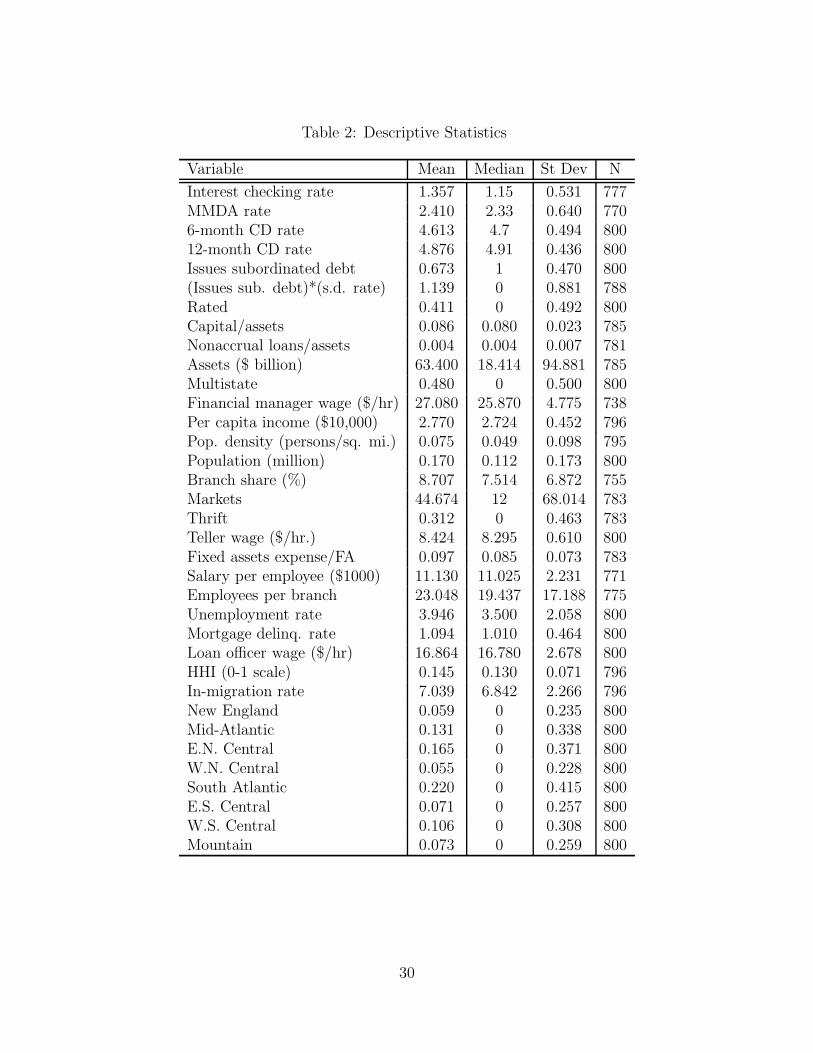
Table 2: Descriptive Statistics

Variable Mean Median St Dev N

Interest checking rate 1.357 1.15 0.531 777MMDA rate 2.410 2.33 0.640 7706-month CD rate 4.613 4.7 0.494 80012-month CD rate 4.876 4.91 0.436 800Issues subordinated debt 0.673 1 0.470 800(Issues sub. debt)*(s.d. rate) 1.139 0 0.881 788Rated 0.411 0 0.492 800Capital/assets 0.086 0.080 0.023 785Nonaccrual loans/assets 0.004 0.004 0.007 781Assets ($ billion) 63.400 18.414 94.881 785Multistate 0.480 0 0.500 800Financial manager wage ($/hr) 27.080 25.870 4.775 738Per capita income ($10,000) 2.770 2.724 0.452 796Pop. density (persons/sq. mi.) 0.075 0.049 0.098 795Population (million) 0.170 0.112 0.173 800Branch share (%) 8.707 7.514 6.872 755Markets 44.674 12 68.014 783Thrift 0.312 0 0.463 783Teller wage ($/hr.) 8.424 8.295 0.610 800Fixed assets expense/FA 0.097 0.085 0.073 783Salary per employee ($1000) 11.130 11.025 2.231 771Employees per branch 23.048 19.437 17.188 775Unemployment rate 3.946 3.500 2.058 800Mortgage delinq. rate 1.094 1.010 0.464 800Loan officer wage ($/hr) 16.864 16.780 2.678 800HHI (0-1 scale) 0.145 0.130 0.071 796In-migration rate 7.039 6.842 2.266 796New England 0.059 0 0.235 800Mid-Atlantic 0.131 0 0.338 800E.N. Central 0.165 0 0.371 800W.N. Central 0.055 0 0.228 800South Atlantic 0.220 0 0.415 800E.S. Central 0.071 0 0.257 800W.S. Central 0.106 0 0.308 800Mountain 0.073 0 0.259 800

30

Table 3: OLS Regression Results

Interest Checking MMDA 6-month CD 12-month CDVariable Coef. Std. Err. Coef. Std. Err. Coef. Std. Err. Coef. Std. Err.

Intercept 3.724** 0.436 4.386** 0.548 6.689** 0.427 6.782** 0.357Issues sub. debt 0.108** 0.047 -0.108* 0.060 -0.060 0.047 0.028 0.039(Issues sub.)*(rate) -0.747 1.108 -0.975 1.405 -1.832* 1.104 -0.951 0.922Rated -0.007 0.048 0.018 0.064 0.057 0.048 0.018 0.040Capital/assets 1.064 0.802 2.690** 1.001 -0.681 0.784 -1.372** 0.655Nonaccr. loans/assets 6.396* 3.401 9.948** 3.112 4.312* 2.447 4.919** 2.044ln(Assets ($1000)) -0.122** 0.014 -0.089** 0.018 -0.063** 0.013 -0.065** 0.011Multistate -0.009 0.044 0.104* 0.057 0.010 0.044 0.004 0.037Fin. mgr. wage ($/hr) -1.055* 0.569 0.717 0.720 0.800 0.567 0.559 0.474PCI ($10,000) 0.022 0.058 -0.003 0.075 -0.003 0.058 0.030 0.048Pop. density 0.117 0.320 0.192 0.402 -0.553* 0.317 -0.405 0.265Population (million) -0.216 0.170 -0.077 0.213 0.036 0.168 -0.007 0.140Branch share (%) 0.004 0.003 -0.004 0.004 -0.011** 0.003 -0.010** 0.003Markets -0.051 0.371 -1.125** 0.487 0.162 0.366 -0.438 0.306Thrift 0.098* 0.056 0.195** 0.071 0.199** 0.055 0.162** 0.046Teller wage ($/hr.) -4.146 4.628 -11.538** 5.840 -13.893** 4.582 -13.595** 3.826Fixed assets exp./FA -0.951** 0.373 0.573 0.448 -0.324 0.353 -0.335 0.295Salary/emp. ($1000) -0.004 0.009 0.033** 0.012 0.021** 0.009 0.024** 0.008Employees/branch 0.002** 0.001 0.001 0.001 0.001 0.001 0.000 0.001Unemployment rate -0.004 0.013 -0.015 0.016 -0.013 0.012 -0.003 0.010Mortgage delinq. rate -0.129** 0.060 -0.363** 0.076 -0.091 0.060 -0.134** 0.050Loan ofcr. wage ($/hr.) 2.069** 0.862 0.909 1.088 1.306 0.847 1.522** 0.707HHI (0-1 scale) -0.586** 0.297 -0.661* 0.377 0.053 0.293 -0.012 0.245In-migration rate 0.271 1.086 0.321 1.387 0.804 1.079 1.029 0.901New England -0.512** 0.157 -0.113 0.199 -0.193 0.157 -0.047 0.131Mid-Atlantic -0.147* 0.083 -0.057 0.104 -0.557** 0.081 -0.142** 0.068E.N. Central -0.051 0.091 -0.131 0.115 -0.368** 0.091 -0.265** 0.076W.N. Central -0.116 0.108 -0.085 0.136 -0.332** 0.107 -0.264** 0.090South Atlantic -0.101 0.075 -0.081 0.095 -0.364** 0.074 -0.254** 0.062E.S. Central 0.140 0.102 0.130 0.132 -0.248** 0.101 -0.044 0.085W.S. Central 0.013 0.084 -0.035 0.105 -0.460** 0.083 -0.318** 0.069Mountain 0.108 0.094 0.184 0.119 -0.223** 0.094 -0.170** 0.079Adjusted R2 0.379 0.341 0.309 0.375N 678 672 695 695

**= significant at the 5% level; *= significant at the 10% level

31

Table 4: Random Effects Regression Results

Interest Checking MMDA 6-month CD 12-month CDVariable Coef. Std. Err. Coef. Std. Err. Coef. Std. Err. Coef. Std. Err.

Intercept 4.018** 0.408 4.444** 0.545 5.951** 0.401 6.193** 0.330Issues sub. debt 0.109 0.072 -0.091 0.076 -0.059 0.059 0.039 0.046(Issues sub.)*(rate) -0.601 2.619 -0.808 2.499 -1.322 2.021 -0.416 1.520Rated -0.011 0.085 0.040 0.090 -0.066 0.070 -0.115** 0.055Capital/assets 0.995 1.094 2.793** 1.177 -0.806 0.908 -1.184* 0.715Nonaccr. loans/assets 6.141 4.160 8.796** 3.603 2.447 2.801 3.796* 2.197ln(Assets ($1000)) -0.112** 0.020 -0.085** 0.022 -0.032* 0.017 -0.036** 0.013Multistate -0.021 0.072 0.117 0.076 -0.020 0.060 -0.014 0.046Fin. mgr. wage ($/hr) -0.988 0.750 0.215 0.874 -0.760 0.670 -0.525 0.534PCI ($10,000) 0.041 0.036 0.027 0.065 0.004 0.045 0.020 0.039Pop. density -0.012 0.237 0.016 0.376 -0.597** 0.276 -0.514** 0.232Population (million) -0.088 0.104 0.016 0.180 0.126 0.130 0.048 0.111Branch share (%) 0.004* 0.002 -0.010** 0.004 -0.013** 0.003 -0.010** 0.002Markets -0.317 1.153 -1.426 1.091 1.040 0.883 -0.016 0.662Thrift 0.066 0.082 0.169* 0.089 0.189** 0.069 0.137** 0.054Teller wage ($/hr.) -7.481** 2.959 -13.289** 5.158 -7.366** 3.670 -8.405** 3.135Fixed assets exp./FA -0.454 0.478 0.638 0.503 -0.246 0.389 -0.300 0.307Salary/emp. ($1000) -0.005 0.013 0.033** 0.014 0.025** 0.011 0.026** 0.008Employees/branch 0.002 0.001 0.001 0.002 0.002 0.001 0.001 0.001Unemployment rate -0.004 0.007 -0.007 0.013 -0.003 0.009 -0.001 0.008Mortgage delinq. rate -0.206** 0.041 -0.365** 0.069 -0.090* 0.050 -0.135** 0.043Loan ofcr. wage ($/hr.) 1.397** 0.580 1.223 0.964 0.709 0.690 1.168** 0.586HHI (0-1 scale) -0.569** 0.209 -0.550 0.345 -0.017 0.248 -0.131 0.209In-migration rate -0.697 0.663 0.811 1.187 1.129 0.837 0.786 0.718New England -0.193 0.127 -0.035 0.190 0.002 0.141 0.089 0.117Mid-Atlantic -0.079 0.070 -0.039 0.105 -0.281** 0.077 0.053 0.064E.N. Central -0.089 0.070 -0.203* 0.112 -0.225** 0.082 -0.138** 0.069W.N. Central -0.113 0.083 -0.129 0.132 -0.179* 0.097 -0.160** 0.081South Atlantic -0.088 0.061 -0.141 0.095 -0.187** 0.070 -0.115* 0.059E.S. Central 0.189** 0.081 0.069 0.131 -0.103 0.094 0.049 0.079W.S. Central 0.015 0.070 -0.099 0.108 -0.315** 0.080 -0.218** 0.066Mountain 0.038 0.060 0.099 0.105 -0.202** 0.076 -0.139** 0.065σu 0.46 0.40 0.33 0.24σe 0.20 0.38 0.27 0.23ρ 0.85 0.52 0.60 0.51N 678 672 695 695

**= significant at the 5% level; *= significant at the 10% level

32

A Comparative Static Results

A.1 Wholesale Funds Rate

First, consider the effect on the switch point DR of an incremental change in the wholesale

funds rate. From (5), implicit differentiation gives

∂DR

∂rw

=1

2 r′R + DR r′′R> 0. (A1)

The level of loans (and retail deposits) at which the bank switches from retail to wholesale

deposits at the margin is increasing in the wholesale funds rate.

The effect of the wholesale funds rate on retail deposit supply is

∂D∗

R

∂rW

=

0 if L∗ ≤ DR,

∂DR

∂rwotherwise.

(A2)

That is, when wholesale funds are used, an increase in the wholesale rate increases equilibrium

retail deposits supplied. For lending below the switch point DR, the wholesale funds rate

has no effect on retail deposits. Upward-sloping retail deposit supply implies

∂rR(D∗

R)

∂rW

= 0 if L∗ ≤ DR,

> 0 otherwise.(A3)

The retail deposit rate is increasing in the wholesale funds rate if wholesale funds are being

purchased; otherwise, it is unaffected by the wholesale rate.

Now consider the effect of rW on total lending:

∂L∗

∂rW

=

0 if L∗ ≤ DR,

12 r′

L+L∗ r′′

L

otherwise.(A4)

The third assumption on loan demand in equation (3) guarantees that the second case in

33

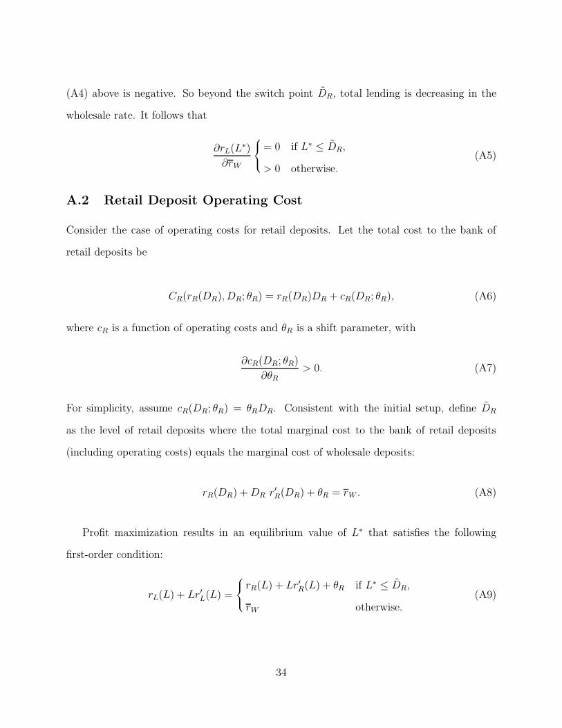
(A4) above is negative. So beyond the switch point DR, total lending is decreasing in the

wholesale rate. It follows that

∂rL(L∗)

∂rW

= 0 if L∗ ≤ DR,

> 0 otherwise.(A5)

A.2 Retail Deposit Operating Cost

Consider the case of operating costs for retail deposits. Let the total cost to the bank of

retail deposits be

CR(rR(DR), DR; θR) = rR(DR)DR + cR(DR; θR), (A6)

where cR is a function of operating costs and θR is a shift parameter, with

∂cR(DR; θR)

∂θR

> 0. (A7)

For simplicity, assume cR(DR; θR) = θRDR. Consistent with the initial setup, define DR

as the level of retail deposits where the total marginal cost to the bank of retail deposits

(including operating costs) equals the marginal cost of wholesale deposits:

rR(DR) + DR r′R(DR) + θR = rW . (A8)

Profit maximization results in an equilibrium value of L∗ that satisfies the following

first-order condition:

rL(L) + Lr′L(L) =

rR(L) + Lr′R(L) + θR if L∗ ≤ DR,

rW otherwise.(A9)

34

Implicit differentiation gives

∂L∗

∂θR

=

12r′

L+L∗r′′

L−[2r′

R+L∗r′′

L]< 0 if L∗ ≤ DR,

0 otherwise.(A10)

Thus, an increase in the marginal cost of retail deposits results in a lower level of total lending

if no wholesale deposits are employed, and no change if wholesale deposits are funding loans

at the margin.

The comparative statics for DR and D∗

R are:

∂DR

∂θR

=−1

2r′R + DRr′′R< 0, (A11)

∂D∗

R

∂θR

=

∂L∗

∂θR< 0 if L∗ ≤ DR,

0 otherwise,(A12)

Thus, retail deposits decrease from an increase in θR for retail deposits below the switch

point, and do not vary with retail deposit operating costs if wholesale funds are being used.

A.3 Wholesale Deposit Operating Cost

Now consider the original model with the addition of a constant marginal operating cost of

wholesale funds θW . Define DR to satisfy

rR(DR) + DR r′R(DR) = rW + θW . (A13)

Clearly, the effect on equilibrium values is identical to the effect of the wholesale funds rate

rW . The comparative static results for θW are therefore identical to those of rW , and take

35

the same form as the results shown in equations (A1) - (A4). To summarize,

∂L∗

∂θW

=

0 if L∗ ≤ DR,

12r′

L+L∗r′′

L

< 0 otherwise,(A14)

∂DR

∂θW

=1

2r′R + DRr′′R> 0, (A15)

∂D∗

R

∂θW

=

0 if L∗ ≤ DR,

∂DR

∂θW

> 0 otherwise,(A16)

∂

∂θW

(

D∗

W

D∗

R

)

=

0 if L∗ ≤ DR,

1DR

∂L∗

∂θW

− L∗

(DR)2∂DR

∂θW

< 0 otherwise.(A17)

A.4 Loan Operating Cost

Assume the parameter θL shifts loan operating costs by increasing total and marginal cost:

∂cL(L; θL)

∂θL

> 0,

∂

∂θL

(c′L) ≥ 0. (A18)

Define DR as originally defined in equation (5). The comparative statics for θL are

∂L∗

∂θL

=

∂

∂θL(c′

L)

2r′L+L∗r′′

L−(2r′

R+L∗r′′

R)−c′′

L

< 0 if L∗ ≤ DR,∂

∂θL(c′

L)

2r′L+L∗r′′

L−c′′

L

< 0 otherwise,(A19)

∂DR

∂θL

= 0, (A20)

36

∂D∗

R

∂θL

=

∂L∗

∂θL< 0 if L∗ ≤ DR,

0 otherwise.(A21)

A.5 Retail Deposit Supply

Consider a parameter σR that shifts the retail deposit supply function rR(DR; σR). Assume

∂rR

∂σR

< 0,

∂

∂σR

(r′R) ≤ 0, (A22)

where r′R = ∂rR(DR; σR)/∂DR. This implies that σR shifts the supply curve down and right,

without steepening the slope. Define DR to satisfy

rR(DR; σR) + DR r′R(DR; σR) = rW . (A23)

The relevant comparative statics are

∂L∗

∂σR

=

∂rR

∂σR+L∗ ∂

∂σR(r′

R)2r′

L+L∗r′′

L−(2r′

R+L∗r′′

R)> 0 if L∗ ≤ DR,

0 otherwise,

(A24)

∂DR

∂σR

=−[ ∂rR

∂σR+ DR

∂∂σR

(r′R)]

2r′R + DRr′′R> 0, (A25)

∂D∗

R

∂σR

=

∂L∗

∂σR> 0 if L∗ ≤ DR,

∂DR

∂σR> 0 otherwise,

(A26)

∂

∂σR

(

D∗

W

D∗

R

)

=

0 if L∗ ≤ DR,

− L∗

(DR)2∂DR

∂σR< 0 otherwise.

(A27)

37

A.6 Loan Demand

Consider a parameter σL that shifts loan demand rL(L; σL). Assume

∂rL

∂σL

> 0,

∂

∂σL

(r′L) ≥ 0;

that is, σL increases loan demand by shifting the function away from the origin without

flattening the slope. Define DR as was specified in the original model to satisfy

rR(DR) + DR r′R(DR) = rW . (A28)

The comparative statics are as follows:

∂DR

∂σL

= 0, (A29)

∂D∗

R

∂σL

=

∂L∗

∂σL> 0 if L∗ ≤ DR,

∂DR

∂σR

= 0 otherwise,(A30)

∂L∗

∂σL

=

∂rL

∂σL+L∗ ∂

∂σL(r′

L)2r′

L+L∗r′′

L−(2r′

R+L∗r′′

R)> 0 if L∗ ≤ DR,

∂rL

∂σL+L∗ ∂

∂σL(r′

L)2r′

L+L∗r′′

L

> 0 otherwise,

(A31)

38

B Welfare Effects of a Change in the Wholesale Rate

The expressions for surplus to borrowers, depositors and the bank are:

borrower surplus =∫ L∗

0[rL(x)− rL(L∗)] dx, (B1)

depositor surplus =∫ D∗

R

0[rR(D∗

R)− rR(x)] dx,

bank surplus =∫ DR

0[rL(L∗)− rR(DR)] dx +

∫ L∗

DR

[rL(L∗)− rW ] dx

= rL(L∗) L∗ − rR(DR) DR − rW (L∗ − DR).

Differentiating the terms above with respect to rW gives

∂(borrower surplus)

∂rW

= −L∗ r′L(L∗)∂L∗

∂rW

< 0, (B2)

∂(depositor surplus)

∂rW

= DR r′R(DR)∂DR

∂rW

> 0, (B3)

∂(bank surplus)

∂rW

= −(L∗ − DR) = −D∗

W < 0. (B4)

A higher wholesale funds rate therefore benefits retail depositors, but decreases the welfare

of borrowers and the bank. The sum of the derivatives above gives the derivative of total

surplus with respect to the wholesale rate. Substituting the terms in (A1) and (A4), the

derivative is

∂(total surplus)

∂rW

= DR

1 +1

2 + DRr′′R

(DR)

r′R

(DR)

− L∗

1 +1

2 + L∗r′′L(L∗)

r′L(L∗)

. (B5)

Hence, the effect on total surplus of the wholesale funds rate depends on the relative

curvature and magnitudes of retail deposit supply and loan demand. With symmetric cur-

vature of these functions, the gains to borrowers from a drop in rW exceed the loss to retail

depositors.

39

C Markets included in the Sample

Market State Market Frequency

1 Albany New York 102 Albuquerque New Mexico 53 Allentown - Bethlehem Pennsylvania 74 Anchorage Alaska 45 Atlanta Georgia 106 Augusta, GA - Aiken, SC Georgia 47 Austin - San Marcos Texas 48 Bakersfield California 89 Baltimore Maryland 1010 Baton Rouge Louisiana 411 Billings Montana 412 Birmingham Alabama 613 Boise Idaho 414 Boston Massachusetts 1015 Bristol - Kingsport Tennessee 416 Buffalo New York 917 Burlington Vermont 518 Canton - Massillon Ohio 419 Casper - Cheyenne Wyoming 420 Charleston - North Charleston South Carolina 421 Charleston West Virginia 422 Charlotte North Carolina 1023 Chattanooga Tennessee 524 Chicago Illinois 1025 Cincinnati Ohio 1026 Cleveland Ohio 1027 Colorado Springs Colorado 628 Columbia South Carolina 429 Columbus Ohio 1030 Concord - Manchester New Hampshire 431 Dallas Texas 1032 Dayton Ohio 933 Daytona Beach Florida 634 Denver - Boulder - Greeley Colorado 1035 Des Moines Iowa 436 Detroit Michigan 1037 El Paso Texas 438 Fargo North Dakota 439 Fort Wayne Indiana 4

continued on next page

40

Market State Market Frequency

40 Fresno California 741 Grand Rapids Michigan 1142 Greensboro North Carolina 643 Greenville - Spartanburg South Carolina 844 Harrisburg - Lebanon - York Pennsylvania 445 Hartford Connecticut 1046 Honolulu Hawaii 447 Houston Texas 1048 Indianapolis Indiana 1049 Jackson Mississippi 650 Jacksonville Florida 1051 Kalamazoo - Battle Creek Michigan 452 Kansas City Kansas 1053 Kansas City Missouri 654 Knoxville Tennessee 455 Lakeland - Winter Haven Florida 456 Lancaster - Reading Pennsylvania 657 Lansing - East Lansing Michigan 458 Las Vegas Nevada 559 Lexington Kentucky 460 Little Rock Arkansas 461 Los Angeles California 1062 Louisville Kentucky 1063 Madison Wisconsin 464 McAllen - Edinburg - Mission Texas 465 Melbourne - Titusville - Palm Bay Florida 466 Memphis Tennessee 967 Miami/Ft. Lauderdale Florida 1268 Milwaukee - Racine Wisconsin 1069 Minneapolis - St. Paul Minnesota 1070 Mobile Alabama 471 Modesto California 672 Nashville Tennessee 1073 New Orleans Louisiana 1074 New York New York 1075 Newark New Jersey 1076 Norfolk - Virginia Beach Virginia 1077 Oklahoma City Oklahoma 1078 Omaha Nebraska 479 Orlando Florida 1080 Philadelphia Pennsylvania 1081 Phoenix - Mesa Arizona 982 Pittsburgh Pennsylvania 10

continued on next page

41

Market State Market Frequency

83 Portland Maine 484 Portland Oregon 985 Providence Rhode Island 1086 Raleigh - Durham - Chapel Hill North Carolina 987 Rapid City - Sioux Falls South Dakota 388 Richmond Virginia 1089 Rochester New York 1190 Sacramento California 1091 Saginaw - Bay City - Midland Michigan 492 Salt Lake City Utah 993 San Antonio Texas 994 San Diego California 1095 San Francisco California 1096 Sarasota - Bradenton Florida 697 Scranton - Wilkes Barre Pennsylvania 498 Seattle Washington 1099 Shreveport - Bossier City Louisiana 4100 Spokane Washington 4101 Springfield Massachusetts 4102 St. Louis Missouri 10103 Stockton - Lodi California 5104 Syracuse New York 11105 Tampa - St. Petersburg Florida 10106 Toledo Ohio 4107 Tucson Arizona 4108 Tulsa Oklahoma 11109 Washington District of Col. 10110 West Palm Beach Florida 10111 Wichita Kansas 5112 Wilmington Delaware 5113 Youngstown - Warren - Akron Ohio 4

Total Observations 806

42

References

Adams, R., L. Roller, and R. Sickles, “Measuring market power for outputs and inputs:

An empirical application to banking,” 2002. FEDS working paper 2002-52, Federal

Reserve Board.

Amel, D. and M. Starr-McCluer, “Market definition in banking: recent evidence,” The

Antitrust Bulletin, 2002, Spring, 63–89.

and T. Hannan, “Establishing banking market definitions through estimation of

residual deposit supply equations,” Journal of Banking and Finance, 1999, 23 (11),

1667–1690.

Berger, A. and D. Humphrey, “Measurement and efficiency issues in commercial bank-

ing,” in Z. Griliches, ed., Output Measurement in the Service Sectors, National Bureau

of Economic Research, Studies in Income and Wealth, Vol. 56, Chicago: University of

Chicago Press, 1992, pp. 245–279.

and T. Hannan, “The price-concentration relationship in banking,” Review of Eco-

nomics and Statistics, 1989, 71 (2), 291–299.

Dick, A., “Demand estimation and market power in the banking industry,” 2002. FEDS

working paper 2002-58, Federal Reserve Board.

Eaton, B. and R. Lipsey, “Product differentiation,” in R. Schmalensee and R. Willig, eds.,

Handbook of Industrial Organization, Amsterdam: North-Holland, 1996, pp. 723–768.

Freixas, X. and J. Rochet, Microeconomics of Banking, Cambridge: MIT Press, 1997.

Frisch, R., Theory of Production, Chicago: Rand McNally and Company, 1965.

43

Furfine, C., “Banks as monitors of other banks: evidence from the overnight federal funds

market,” Journal of Business, 2001, 74 (1), 33–57.

Greene, W., Econometric Analysis, Fourth Edition, New Jersey: Prentice Hall, 2000.

Hancock, D., “The financial firm: Production with monetary and nonmonetary goods,”

Journal of Political Economy, 1985, 93 (5), 859–880.

Hausman, J., “Specification tests in econometrics,” Econometrica, 1978, 46 (6), 1251–1271.

Heitfield, E., “What do interest rate data say about the geography of retail banking mar-

kets?,” The Antitrust Bulletin, 1999, 44 (2), 333–348.

Hughes, J. and L. Mester, “Bank capitalization and cost: evidence of scale economies

in risk management and signaling,” Review of Economics and Statistics, 1998, 80 (2),

314–325.

Jayaratne, J. and D. Morgan, “Capital market frictions and deposit constraints at

banks,” Journal of Money, Credit and Banking, 2000, 32 (1), 74–92.

Kashyap, A. and J. Stein, “What do a million observations on banks say about the

transmission of monetary policy?,” American Economic Review, 2000, 90 (3), 407–428.

Kiser, E., “Household switching behavior at depository institutions: evidence from survey

data,” The Antitrust Bulletin, Winter 2002, 47 (4), 619–640.

Klein, M., “A theory of the banking firm,” Journal of Money, Credit and Banking, 1971,

3, 205–218.

Klemperer, P., “Competition when consumers have switching costs: an overview with ap-

plications to industrial organization, macroeconomics, and international trade,” Review

of Economic Studies, 1995, 62, 515–539.

44

Massoud, N. and D. Bernhardt, “’Rip-off’ ATM Surcharges,” RAND Journal of Eco-

nomics, 2002, 33 (1), 96–115.

Monti, M., “Deposit, credit, and interest rate determination under alternative bank ob-

jectives,” in G. P. Szego and K. Shell, eds., Mathematical methods in investment and

finance, Amsterdam: North-Holland, 1972.

Morgan, D. and K. Stiroh, “Market Discipline of Banks: the Asset Test,” 2000. Working

paper, Federal Reserve Bank of New York.

Prager, R. and T. Hannan, “Do Substantial Horizontal Mergers Generate Significant

Price Effects? Evidence from the Banking Industry,” Journal of Industrial Economics,

1998, 46 (4), 433–52.

Santomero, A., “Modeling the banking firm: a survey,” Journal of Money, Credit and

Banking, 1984, 16 (4), 576–602.

Sealey, C. and J. Lindley, “Inputs, outputs, and a theory of production and cost at

depository financial institutions,” Journal of Finance, 1977, 32 (4), 1251–1266.

Sharpe, S., “The effect of consumer switching costs on prices: A theory and its application

to the bank deposit market,” Review of Industrial Organization, 1997, 12 (1), 79–94.

Tobin, J., “Chapter 8 - The theory of commercial banking,” 1958. Unpublished manuscript.

45