11 Formulating and Solving Integer Programs -...
74
261 11 Formulating and Solving Integer Programs “To be or not to be” is true. -G. Boole 11.1 Introduction In many applications of optimization, one would really like the decision variables to be restricted to integer values. One is likely to tolerate a solution recommending GM produce 1,524,328.37 Chevrolets. No one will mind if this recommendation is rounded up or down. If, however, a different study recommends the optimum number of aircraft carriers to build is 1.37, then a lot of people around the world will be very interested in how this number is rounded. It is clear the validity and value of many optimization models could be improved markedly if one could restrict selected decision variables to integer values. All good commercial optimization modeling systems are augmented with a capability that allows the user to restrict certain decision variables to integer values. The manner in which the user informs the program of this requirement varies from program to program. In LINGO, for example, one way of indicating variable X is to be restricted to integer values is to put it in the model the declaration as: @GIN(X). The important point is it is straightforward to specify this restriction. We shall see later that, even though easy to specify, sometimes it may be difficult to solve problems with this restriction. The methods for formulating and solving problems with integrality requirements are called integer programming. 11.1.1 Types of Variables One general classification is according to types of variables: Pure vs. mixed. In a pure integer program, all variables are restricted to integer values. In a mixed formulation, only certain of the variables are integer; whereas, the rest are allowed to be continuous. 0/1 vs. general. In many applications, the only integer values allowed are 0/1. Therefore, some integer programming codes assume integer variables are restricted to the values 0 or 1. The integrality enforcing capability is perhaps more powerful than the reader at first realizes. A frequent use of integer variables in a model is as a zero/one variable to represent a go/no-go decision. It is probably true that the majority of real world integer programs are of the zero/one variety.
-
Upload
phungkhanh -
Category
Documents
-
view
235 -
download
1
Transcript of 11 Formulating and Solving Integer Programs -...
261
11
Formulating and Solving Integer Programs
“To be or not to be” is true. -G. Boole
11.1 Introduction In many applications of optimization, one would really like the decision variables to be restricted to integer values. One is likely to tolerate a solution recommending GM produce 1,524,328.37 Chevrolets. No one will mind if this recommendation is rounded up or down. If, however, a different study recommends the optimum number of aircraft carriers to build is 1.37, then a lot of people around the world will be very interested in how this number is rounded. It is clear the validity and value of many optimization models could be improved markedly if one could restrict selected decision variables to integer values. All good commercial optimization modeling systems are augmented with a capability that allows the user to restrict certain decision variables to integer values. The manner in which the user informs the program of this requirement varies from program to program. In LINGO, for example, one way of indicating variable X is to be restricted to integer values is to put it in the model the declaration as: @GIN(X). The important point is it is straightforward to specify this restriction. We shall see later that, even though easy to specify, sometimes it may be difficult to solve problems with this restriction. The methods for formulating and solving problems with integrality requirements are called integerprogramming.
11.1.1 Types of Variables One general classification is according to types of variables:
Pure vs. mixed. In a pure integer program, all variables are restricted to integer values. In a mixed formulation, only certain of the variables are integer; whereas, the rest are allowed to be continuous.
0/1 vs. general. In many applications, the only integer values allowed are 0/1. Therefore, some integer programming codes assume integer variables are restricted to the values 0 or 1.
The integrality enforcing capability is perhaps more powerful than the reader at first realizes. A frequent use of integer variables in a model is as a zero/one variable to represent a go/no-go decision. It is probably true that the majority of real world integer programs are of the zero/one variety.
262 Chapter 11 Formulating & Solving Integer Programs
11.2 Exploiting the IP Capability: Standard Applications You will frequently encounter LP problems with the exception of just a few combinatorial complications. Many of these complications are fairly standard. The next several sections describe many of the standard complications along with the methods for incorporating them into an IP formulation. Most of these complications only require the 0/1 capability rather than the general integer capability. Binary variables can be used to represent a wide variety of go/no-go, or make-or-buy decisions. In the latter use, they are sometimes referred to as “Hamlet” variables as in: “To buy or not to buy, that is the question”. Binary variables are sometimes also called Boolean variables in honor of the logician George Boole. He developed the rules of the special algebra, now known as Boolean algebra, for manipulating variables that can take on only two values. In Boole’s case, the values were “True” and “False”. However, it is a minor conceptual leap to represent “True” by the value 1 and “False” by the value 0. The power of these methods developed by Boole is undoubtedly the genesis of the modern compliment: “Strong, like Boole.”
11.2.1 Binary Representation of General Integer Variables Some algorithms apply to problems with only 0/1 integer variables. Conceptually, this is no limitation, as any general integer variable with a finite range can be represented by a set of 0/1 variables. For example, suppose X is restricted to the set [0, 1, 2,...,15]. Introduce the four 0/1 variables: y1, y2, y3,
and y4. Replace every occurrence of X by y1 + 2 y2 + 4 y3 + 8 y4. Note every possible integer in
[0, 1, 2, ..., 15] can be represented by some setting of the values of y1, y2, y3, and y4. Verify that, if the
maximum value X can take on is 31, you will need 5 0/1 variables. If the maximum value is 63, you will need 6 0/1 variables. In fact, if you use k 0/1 variables, the maximum value that can be represented is 2k-1. You can write: VMAX = 2k-1. Taking logs, you can observe that the number of 0/1 variables required in this so-called binary expansion is approximately proportional to the log of the maximum value X can take on. Although this substitution is valid, it should be avoided if possible. Most integer programming algorithms are not very efficient when applied to models containing this substitution.
11.2.2 Minimum Batch Size Constraints When there are substantial economies of scale in undertaking an activity regardless of its level, many decision makers will specify a minimum “batch” size for the activity. For example, a large brokerage firm may require that, if you buy any bonds from the firm, you must buy at least 100. A zero/one variable can enforce this restriction as follows. Let:
x = activity level to be determined (e.g., no. of bonds purchased), y = a zero/one variable = 1, if and only if x > 0, B = minimum batch size for x (e.g., 100), and U = known upper limit on the value of x.
The following two constraints enforce the minimum batch size condition:
x Uy
By x.
If y = 0, then the first constraint forces x = 0. While, if y = 1, the second constraint forces x to be at least B. Thus, y acts as a switch, which forces x to be either 0 or greater than B. The constant U should be chosen with care. For reasons of computational efficiency, it should be as small as validly possible.

Formulating & Solving Integer Problems Chapter 11 263
Some IP packages allow the user to directly represent minimum batch size requirements by way of so-called semi-continuous variables. A variable x is semi-continuous if it is either 0 or in the range
B x . No binary variable need be explicitly introduced.
11.2.3 Fixed Charge Problems A situation closely related to the minimum batch size situation is one where the cost function for an activity is of the fixed plus linear type indicated in Figure 11.1:
Figure 11.1 A Fixed Plus Linear Cost Curve
Slope c
xU
K
00
Cost
Define x, y, and U as before, and let K be the fixed cost incurred if x > 0. Then, the following components should appear in the formulation:
Minimize Ky + cx + . . . subject to
x Uy . . .
The constraint and the term Ky in the objective imply x cannot be greater than 0 unless a cost K is incurred. Again, for computational efficiency, U should be as small as validly possible.
11.2.4 The Simple Plant Location Problem The Simple Plant Location Problem (SPL) is a commonly encountered form of fixed charge problem. It is specified as follows:
n = the number of sites at which a plant may be located or opened, m = the number of customer or demand points, each of which must be assigned to a plant, k = the number of plants which may be opened, fi = the fixed cost (e.g., per year) of having a plant at site i, for i = 1, 2, . . . , n,cij = cost (e.g., per year) of assigning customer j to a plant at site i, for i = 1, 2, . . . , n and
j = 1, 2, ..., m.

264 Chapter 11 Formulating & Solving Integer Programs
The goal is to determine the set of sites at which plants should be located and which site should service each customer. A situation giving rise to the SPL problem is the lockbox location problem encountered by a firm with customers scattered over a wide area. The plant sites, in this case, correspond to sites at which the firm might locate a postal lockbox that is managed by a bank at the site. The customer points would correspond to the, 100 say, largest metropolitan areas in the firm’s market. A customer would mail his or her monthly payments to the closest lockbox. The reason for resorting to multiple lockboxes rather than having all payments mailed to a single site is several days of mail time may be saved. Suppose a firm receives $60 million per year through the mail. The yearly cost of capital to the firm is 10% per year, and it could reduce the mail time by two days. This reduction has a yearly value of about $30,000. The fi for a particular site would equal the yearly cost of having a lockbox at site i regardless of the volume processed through the site. The cost term cij would approximately equal the product: (daily
cost of capital) (mail time in days between i and j) (yearly dollar volume mailed from area j). Define the decision variables:
yi = 1 if a plant is located at site i, else 0, xij = 1 if the customer j is assigned to a plant site i, else 0.
A compact formulation of this problem as an IP is:
Minimize in
1 fi yi + in
1 jm
1 cij xij(1)
subject to in
1 xij = 1 for j = 1 to m, (2)
jm
1 xij myifor i = 1 to n, (3)
in
1 yi = k, (4)
yi = 0 or 1 for i = 1 to n, (5) xij = 0 or 1 for i = 1 to n, j = 1 to m. (6)
The constraints in (2) force each customer j to be assigned to exactly one site. The constraints in (3) force a plant to be located at site i if any customer is assigned to site i. The reader should be cautioned against trying to solve a problem formulated in this fashion because the solution process may require embarrassingly much computer time for all, but the smallest problem. The difficulty arises because, when the problem is solved as an LP (i.e., with the conditions in (5) and (6) deleted), the solution tends to be highly fractional and with little similarity to the optimal IP solution. A “tighter” formulation, which frequently produces an integer solution naturally when solved as an LP, is obtained by replacing (3) by the formula:
xij yi for i = 1 to n, j = 1 to m. (3')
At first glance, replacing (3) by (3') may seem counterproductive. If there are 20 possible plant sites and 60 customers, then the set (3) would contain 20 constraints, whereas set (3') would contain
20 60 = 1,200 constraints. Empirically, however, it appears to be the rule rather than the exception that, when the problem is solved as an LP with (3') rather than (3), the solution is naturally integer.

Formulating & Solving Integer Problems Chapter 11 265
11.2.5 The Capacitated Plant Location Problem (CPL) The CPL problem arises from the SPL problem if the volume of demand processed through a particular plant is an important consideration. In particular, the CPL problem assumes each customer has a known volume and each plant site has a known volume limit on total volume assigned to it. The additional parameters to be defined are:
Dj = volume or demand associated with customer j,Ki = capacity of a plant located at i
The IP formulation is:
Minimize in
1 fi yi + in
1 jm
1 cij xij(7)
subject to in
1 xij = 1 for j = 1 to m (8)
jm
1 Djxij Kiyifor i = 1 to n (9)
xij yi for i = 1 to n, j = 1 to m. (10)
yi = 0 or 1 for i = 1 to n (11) xij = 0 or 1 for i = 1 to n, j = 1 to m. (12)
This is the “single-sourcing” version of the problem. Because the variables xi j are restricted to 0 or 1, each customer must have all of its volume assigned to a single plant. If “split-sourcing” is allowed, then the variables xi j are allowed to be fractional with the interpretation that xi j is the fraction of customer j’s volume assigned to plant site i. In this case, condition (12) is dropped. Split sourcing, considered alone, is usually undesirable. An example is the assignment of elementary schools to high schools. Students who went to the same elementary school prefer to be assigned to the same high school.

266 Chapter 11 Formulating & Solving Integer Programs
Example: Capacitated Plant Location
Some of the points just mentioned will be illustrated with the following example. The Zzyzx Company of Zzyzx, California currently has a warehouse in each of the following cities: (A) Baltimore, (B) Cheyenne, (C) Salt Lake City, (D) Memphis, and (E) Wichita. These warehouses supply customer regions throughout the U.S. It is convenient to aggregate customer areas and consider the customers to be located in the following cities: (1) Atlanta, (2) Boston, (3) Chicago, (4) Denver, (5) Omaha, and (6) Portland, Oregon. There is some feeling that Zzyzx is “overwarehoused”. That is, it may be able to save substantial fixed costs by closing some warehouses without unduly increasing transportation and service costs. Relevant data has been collected and assembled on a “per month” basis and is displayed below:
Cost per Ton-Month Matrix
Demand City
Warehouse
1 2 3 4 5 6
Monthly Supply
Capacity in Tons
Monthly Fixed Cost
A $1675 $400 $685 $1630 $1160 $2800 18 $7,650 B 1460 1940 970 100 495 1200 24 3,500 C 1925 2400 1425 500 950 800 27 3,500 D 380 1355 543 1045 665 2321 22 4,100 E 922 1646 700 508 311 1797 31 2,200
Monthly Demand in Tons 10 8 12 6 7 11
For example, closing the warehouse at A (Baltimore) would result in a monthly fixed cost saving of $7,650. If 5 (Omaha) gets all of its monthly demand from E (Wichita), then the associated
transportation cost for supplying Omaha is 7 311 = $2,177 per month. A customer need not get all of its supply from a single source. Such “multiple sourcing” may result from the limited capacity of each warehouse (e.g., Cheyenne can only process 24 tons per month. Should Zzyzx close any warehouses and, if so, which ones?) We will compare the performance of four different methods for solving, or approximately solving, this problem:
1) Loose formulation of the IP. 2) Tight formulation of the IP. 3) Greedy open heuristic: start with no plants open and sequentially open the plant giving
the greatest reduction in cost until it is worthless to open further plants. 4) Greedy close heuristic: start with all plants open and sequentially close the plant saving
the most money until it is worthless to close further plants.
The advantage of heuristics 3 and 4 is they are easy to apply. The performance of the four methods is as follows:
Method
Objective value: Best
Solution
Computing Time in
SecondsPlantsOpen
Objective value: LP Solution
Loose IP 46,031 3.38 A,B,D 35,662
Tight IP 46,031 1.67 A,B,D 46,031
Greedy Open Heuristic 46,943 nil A,B,D,E —
Greedy Close Heuristic 46,443 nil A,C,D,E —

Formulating & Solving Integer Problems Chapter 11 267
Notice, even though the loose IP finds the same optimum as the tight formulation (as it must), it takes about twice as much computing time. For large problems, the difference becomes much more dramatic. Notice for the tight formulation, however, the objective function value for the LP solution is the same as for the IP solution. When the tight formulation was solved as an LP, the solution was naturally integer. The single product dynamic lotsizing problem is described by the following parameters:
n = number of periods for which production is to be planned for a product; Dj = predicted demand in period j, for j = 1, 2, . . . , n;fi = fixed cost of making a production run in period i;hi = cost per unit of product carried from period i to i + 1.
This problem can be cast as a simple plant location problem if we define:
ci j = Dj t i
j 1
ht.
That is, cij is the cost of supplying period j’s demand from period i production. Each period can be thought of as both a potential plant site (period for a production run) and a customer. If, further, there is a finite production capacity, Ki, in period i, then this capacitated dynamic lotsizing problem is a special case of the capacitated plant location problem.
Dual Prices and Reduced Costs in Integer Programs
Dual prices and reduced costs in solution reports for integer programs have a restricted interpretation. For first time users of IP, it is best to simply disregard the reduced cost and dual price column in the solution report. For the more curious, the dual prices and reduced costs in a solution report are obtained from the linear program that remains after all integer variables have been fixed at their optimal values and removed from the model. Thus, for a pure integer program (i.e., all variables are required to be integer), you will generally find:
all dual prices are zero, and
the reduced cost of a variable is simply its objective function coefficient (with sign reversed if the objective is MAX).
For mixed integer programs, the dual prices may be of interest. For example, for a plant location problem where the location variables are required to be integer, but the quantity-shipped variables are continuous, the dual prices reported are those from the continuous problem where the locations of plants have been specified beforehand (at the optimal locations).
11.2.6 Modeling Alternatives with the Scenario Approach We may be confronted by alternatives in two different ways: a) we have to choose among two or more alternatives and we want to figure out which is best, or b) nature or the market place will choose one of two or more alternatives, and we are not sure which alternative nature will choose, so we want to analyze all alternatives so we will be prepared to react optimally once we learn which alternative was chosen by nature. Here we consider only situation (a). We call the approach the scenario approach or the disjunctive formulation, see for example Balas(1979) or section 16.2.3 of Martin(1999).

268 Chapter 11 Formulating & Solving Integer Programs
Suppose that if we disregard the alternatives, our variables are simply called x1, x2, …, xn. We call the conditions that must hold if alternative s is chosen, scenario s. Without too much loss of generality, we assume all variables are non-negative. The scenario/disjunctive approach to formulating a discrete decision problem proceeds as follows:
For each scenario s: 1) Write all the constraints that must hold if scenario s is chosen. 2) For all variables in these constraints add a subscript s, to distinguish them from equivalent variables in other scenarios. So xj in scenario s becomes xsj. 3) Add a 0/1 variable, ys, to the model with the interpretation that ys = 1 if scenario s is chosen, else 0. 4) Multiply the RHS constant term of each constraint in scenario s by ys. 5) For each variable xsj that appears in any of the scenario s constraints, add the constraint:
xsj M* ys , where M is a large positive constant. The purpose of this step is to force all variables in scenario s to be 0 if scenario s is not chosen.
Finally, we tie all the scenarios together with:
s ys = 1, i.e., we must choose one scenario; For each variable xj, add the constraint:
xj = s xsj , so xj takes on the value appropriate to which scenario was chosen.
For example, if just after step 1 we had a constraint of the form:
j asj*xj as0,then steps 2-4 would convert it to:
j asj*xsj as0*ys,
The forcing constraints in step 5 are not needed if ys = 0 implies xsj = 0, e.g., if all the asj are nonnegative and the xj are constrained to be nonnegative.
The next section illustrates the scenario approach for representing a decision problem.
11.2.7 Linearizing a Piecewise Linear Function If you ask a vendor to provide a quote for selling you some quantity of material, the vendor will typically offer a quantity discount function that looks something like that shown in figure 11.2

Formulating & Solving Integer Problems Chapter 11 269
Figure 11.2 Quantity Discount Piecewise Linear Cost Curve
h1 h2 h3 h4
quantity
Define: hs, vs = coordinates of the rightmost point of segment s of the piecewise linear function,.
cs = slope of segment s,
Note that segment 1 is the degenerate segment of buying nothing. This example illustrates that we do not require that a piecewise linear function be continuous.
Let us consider the following situation: We pay $50 if we buy anything in a period, plus $2.00/unit if quantity < 100,
$1.90/unit if quantity 100 but < 1000,
$1.80/unit if 1000 but 5000.
We assume hs, vs , cs are constants, and hs hs+1 . It then follows that:
h v c = 0 0 0 100 250 2 1000 1950 1.90 5000 9050 1.80;
v2
v1
v3
v4c4
c3
c2
cost

270 Chapter 11 Formulating & Solving Integer Programs
Let x denote the amount we decide to purchase. Using step 1 of the scenario formulation approach, If segment/scenario 1 is chosen, then cost = 0; x = 0;
If segment/scenario 2 is chosen, then cost = v2 – c2*( h2 - x); [or 250 – 2*(100 - x)],
x h2; [or x 100],
x h1; [or x 0],
Similar constraints apply for scenario/segments 3 and 4. We assume that fractional values, such as x =
99.44 are allowed, else we would write x 99 rather than x 100 above.
If we apply steps 2-4 of the scenario formulation method, then we get: For segment/scenario 1 is chosen, then cost1 = 0; x1 = 0; If segment/scenario 2 is chosen, then cost2 = v2* y2 – c2*h2*y2 + c2*x2; [ or cost2 = 50* y2 + 2*x2],
x2 h2*y2; [ or x2 100*y2],
x2 h1*y2; [ or x2 0*y2 ],
If segment/scenario 3 is chosen, then cost3 = v3* y3 – c3*h3*y3 + c3*x3; [ or cost3 = 50* y3 + 1.9*x3],
x3 h3*y3; [ or x3 1000*y3],
x3 h2*y3; [ or x3 100*y3],
If segment/scenario 4 is chosen, then cost4 = v4* y4 – c4*h4*y4 + c4*x4; [or cost4 = 50* y3 + 1.8*x4 ]
x4 h4*y4; [ or x3 5000*y4],
x4 h3*y4; [ or x3 1000*y4],
We must choose one of the four segments, so: y1 + y2 + y3 + y4 = 1; y1, y2, y3, y4 = 0 or 1;
and the true quantity and cost are found with: x1+ x2+ x3+ x4 = x;
cost1 + cost2 +cost3 + cost4 = cost;
Example
The previous quantity discount example illustrated what is called an “all units discount”. Sometimes, a vendor will instead quote an incremental units discount, in which the discount applies only to the units above a threshold. The following example illustrates. There is a fixed cost of $150 for placing an order. The first 1,000 gallons of the product can be purchased for $2 per gallon. The price drops to $1.90 per gallon for anything in excess of 1,000 gallons. At most, 5,000 gallons will be purchased. Using the scenario/disjunctive approach again.

Formulating & Solving Integer Problems Chapter 11 271
Define the variables:
y0 = 1 if nothing is bought, else 0; y1 =1 if more than 0, but no more than 1000, gallons are purchased, else 0;y2 = 1 if more than 1,000 gallons are purchased, else 0; x1 = gallons purchased if no more than 1,000 gallons are purchased; x2 = gallons purchased if more than 1,000 gallons are purchased.
The formulation would include:
MIN = cost + ...; !s.t.;! Segment/scenario 1; cost1 = 150*y1 + 2*x1; x1 <= 1000 *y1; ! Segment/scenario 2; cost2 = (150 + (2.0-1.9)*1000)*y1 + 1.9*x2; x2 >= 1000*y2; x2 <= 5000*y2; ! Choose a scenario/segment;
y0 + y1 + y2 = 1; cost1 + cost2 = cost; x1 + x2 = x; @BIN(y1); @BIN(y2);
! Plus other constraints & variables to complete model;
11.2.8 Converting to Separable Functions The previous method is applicable only to nonlinear functions of one variable. There are some standard methods available for transforming a function of several variables, so a function is obtained that is additively separable in the transformed variables. The most common such transformation is for converting a product of two variables into separable form. For example, given the function:
x1 * x2 ,
add the linear constraints:
y1 = (x1 + x2)/2
y2 = (x1 x2)/2.
Then, replace every instance of x1 * x2 by the term y12 y2
2. That is, the claim is:
x1 * x2 = y12 y2
2.
The justification is observed by noting:
y12 y2
2 = (x12+ 2 * x1 * x2 + x2
2)/4
(x12 2 * x1 * x2 + x2
2)/4
= 4 * x1 * x2 /4 = x1 * x2
This example suggests that, any time you have a product of two variables, you can add two new variables to the model and replace the product term by a sum of two squared variables. If you have n
original variables, you could have up to n(n 1)/2 cross product terms. This suggests that you might

272 Chapter 11 Formulating & Solving Integer Programs
need up to n(n 1) new variables to get rid of all cross product terms. In fact, under certain conditions, the above ideas can be generalized (using the technique of Cholesky factorization), so only n new variables are needed.
11.3 Outline of Integer Programming Methods The time a computer requires to solve an IP may depend dramatically on how you formulated it. It is, therefore, worthwhile to know a little about how IPs are solved. There are two general approaches for solving IPs: “cutting plane” methods and “branch-and-bound” (B & B) method. For a comprehensive introduction to integer programming solution methods, see Nemhauser and Wolsey (1988), and Wolsey (1998). Most commercial IP programs use the B & B method, but aided by some cutting plane features. Fortunately for the reader, the B & B method is the easier to describe. In most general terms, B & B is a form of intelligent enumeration. More specifically, B & B first solves the problem as an LP. If the LP solution is integer valued in the integer variables, then no more work is required. Otherwise, B & B resorts to an intelligent search of all possible ways of rounding the fractional variables. We shall illustrate the application of the branch-and-bound method with the following problem:
MAX= 75 * X1 + 6 * X2 + 3 * X3 + 33 * X4; 774 * X1 + 76 * X2 + 22 * X3 + 42 * X4 <= 875; 67 * X1 + 27 * X2 + 794 * X3 + 53 * X4 <= 875; @BIN( X1); @BIN( X2); @BIN( X3); @BIN( X4);
The search process a computer might follow in finding an integer optimum is illustrated in
Figure 11.4. First, the problem is solved as an LP with the constraints X1, X2, X3, X4 1. This solution is summarized in the box labeled 1. The solution has fractional values for X2 and X3 and is, therefore, unacceptable. At this point, X2 is arbitrarily selected and the following reasoning is applied. At the integer optimum, X2 must equal either 0 or 1.

Formulating & Solving Integer Problems Chapter 11 273
Figure 11.4 Branch-and-Bound Search Tree
Therefore, replace the original problem by two new subproblems. One with X2 constrained to equal 1 (box or node 2) and the other with X2 constrained to equal 0 (node 8). If we solve both of these new IPs, then the better solution must be the best solution to the original problem. This reasoning is the motivation for using the term “branch”. Each subproblem created corresponds to a branch in an enumeration tree. The numbers to the upper left of each node indicate the order in which the nodes (or equivalently, subproblems) are examined. The variable Z is the objective function value. When the subproblem with X2 constrained to 1 (node 2) is solved as an LP, we find X1 and X3 take fractional values. If we argue as before, but now with variable X1, two new subproblems are created:
Node 7) one with X1 constrained to 0 , and Node 3) one with X1 constrained to 1.
This process is repeated with X4 and X3 until node 5. At this point, an integer solution with Z = 81 is found. We do not know this is the optimum integer solution, however, because we must still look at subproblems 6 through 10. Subproblem 6 need not be pursued further because there are no feasible solutions having all of X2, X1, and X4 equal to 1. Subproblem 7 need not be pursued further because it has a Z of 42, which is worse than an integer solution already in hand.

274 Chapter 11 Formulating & Solving Integer Programs
At node 9, a new and better integer solution with Z = 108 is found when X3 is set to 0. Node 10 illustrates the source for the “bound” part of “branch-and-bound”. The solution is fractional. However, it is not examined further because the Z-value of 86.72 is less than the 108 associated with an integer solution already in hand. The Z-value at any node is a bound on the Z-value at any offspring node. This is true because an offspring node or subproblem is obtained by appending a constraint to the parent problem. Appending a constraint can only hurt. Interpreted in another light, this means the Z-values cannot improve as one moves down the tree. The tree presented in the preceding figure was only one illustration of how the tree might be searched. Other trees could be developed for the same problem by playing with the following two degrees of freedom:
(a) Choice of next node to examine, and (b) Choice of how the chosen node is split into two or more subnodes.
For example, if nodes 8 and then 9 were examined immediately after node 1, then the solution with Z = 108 would have been found quickly. Further, nodes 4, 5, and 6 could then have been skipped because the Z-value at node 3 (100.64) is worse than a known integer solution (108), and, therefore, no offspring of node 3 would need examination. In the example tree, the first node is split by branching on the possible values for X2. One could have just as well chosen X3 or even X1 as the first branching variable. The efficiency of the search is closely related to how wisely the choices are made in (a) and (b) above. Typically, in (b) the split is made by branching on a single variable. For example, if, in the continuous solution, x = 1.6, then the obvious split is to create two subproblems. One with the
constraint x 1, and the other with the constraint x 2. The split need not be made on a single variable. It could be based on an arbitrary constraint. For example, the first subproblem might be based
on the constraint x1 + x2 + x3 0, while the second is obtained by appending the constraint
x1 + x2 + x3 1. Also, the split need not be binary. For example, if the model contains the constraint y1 + y2 + y3 = 1, then one could create three subproblems corresponding to either y1 = 1, or y2 = 1, or y3 = 1. If the split is based on a single variable, then one wants to choose variables that are “decisive.” In general, the computer will make intelligent choices and the user need not be aware of the details of the search process. The user should, however, keep the general B & B process in mind when formulating a model. If the user has a priori knowledge that an integer variable x is decisive, then for the LINGO program it is useful to place x early in the formulation to indicate its importance. This general understanding should drive home the importance of a “tight” LP formulation. A tight LP formulation is one which, when solved, has an objective function value close to the IP optimum. The LP solutions at the subproblems are used as bounds to curtail the search. If the bounds are poor, many early nodes in the tree may be explicitly examined because their bounds look good even though, in fact, these nodes have no good offspring.
11.4 Computational Difficulty of Integer Programs Integer programs can be very difficult to solve. This is in marked contrast to LP problems. The solution time for an LP is fairly predictable. For an LP, the time increases approximately proportionally with the number of variables and approximately with the square of the number of constraints. For a given IP problem, the time may in fact decrease as the number of constraints is increased. As the number of integer variables is increased, the solution time may increase dramatically. Some small IPs (e.g., 6 constraints, 60 variables) are extremely difficult to solve. Just as with LPs, there may be alternate IP formulations of a given problem. With IPs, however, the solution time generally depends critically upon the formulation. Producing a good IP formulation

Formulating & Solving Integer Problems Chapter 11 275
requires skill. For many of the problems in the remainder of this chapter, the difference between a good formulation and a poor formulation may be the difference between whether the problem is solvable or not.
11.4.1 NP-Complete Problems Integer programs belong to a class of problems known as NP-hard. We may somewhat loosely think of NP as meaning "not polynomial". This means that there is no known algorithm of solving these problems such that the computational effort at worst increases as a polynomial in the problem size. For our purposes, we will say that an algorithm runs in polynomial time if there is a positive constant k,such that the time to solve a problem of size n is proportional to nk. For example, sorting a set of nnumbers can easily be done in (polynomial) time proportional to n2,(n log(n) if one is careful), whereas solving an integer program in n zero/one variables may, in the worst case, take (exponential) time proportional to 2n. There may be a faster way, but no one has published an algorithm for integer programs that is guaranteed to take polynomial time on every problem presented to it. The terms NP-complete and P-complete apply to problems that can be stated as "yes/no" or feasibility problems. The yes/no variation of an optimization problem would be a problem of the form: Is there a feasible solution to this problem with cost less-than-or-equal-to 1250. In an optimization problem, we want a feasible solution with minimum cost. Khachian (1979) showed that the feasibility version of LP is solvable in polynomial time. So, we say LP is in P. Integer programming stated in feasibility form, and a wide range of similar problems, belong to a class of problems called NP-complete. These problems have the feature that it is possible to convert any one of these problems into any other NP-complete problem in time that is polynomial in the problem size. Thus, if we can convert problem A into problem B in polynomial time, then solve B in polynomial time, and then convert the solution to B to a valid solution to A in polynomial time, we then have a way of solving A in polynomial time. The notable thing about NP-complete problems is that, if someone develops a guaranteed fast (e.g., polynomial worst case) time method for solving one of these problems, then that someone also has a polynomial time algorithm for every other NP-complete problem. An important point to remember is that the NP-completeness classification is defined in terms of worst case behavior, not average case behavior. For practical purposes, one is interested mainly in average case behavior. The current situation is that the average time to solve many important practical integer programming problems is quite short. The fact that someone may occasionally present us with an extremely difficult integer programming problem does not prevent us from profiting from the fact that a large number of practical integer programs can be solved rapidly. Perhaps the biggest open problem in modern mathematics is whether the problems in the NP-complete class are inherently difficult. This question is cryptically phrased as is: P = NP? Are these problems really difficult, or is it that we are just not smart enough to discover the universally fast algorithm? In fact, a “Millenium prize” of $1,000,000 is offered by the Clay Mathematics Institute, www.claymath.org, for an answer to this question. For a more comprehensive discussion of the NP-complete classification, see Martin (1999).
11.5 Problems with Naturally Integer Solutions and the Prayer Algorithm
The solution algorithms for IP are generally based on first solving the IP as an LP by disregarding the integrality requirements and praying the solution is naturally integer. For example, if x is required to be 0 or 1, the problem is first solved by replacing this requirement by the requirement that simply
0 x 1. When initiating the analysis of a problem in which integer answers are important, it is useful to know beforehand whether the resulting IP will be easy to solve. After the fact, one generally

276 Chapter 11 Formulating & Solving Integer Programs
observes the IP was easy to solve if the objective function values for the LP optimum and the IP optimum were close. About the only way we can predict beforehand the objective function values of the LP and IP will be close is if we know beforehand the LP solution will be almost completely integer valued. Thus, we are interested in knowing what kinds of LPs have naturally integer solutions. The classes of LP problems for which we know beforehand there is a naturally integer optimum have integer right-hand sides and are in one of the classes:
(a) Network LPs, (b) MRP or Integral Leontief LPs, (c) Problems that can be transformed to (a) or (b) by either row operations or taking the dual.
We first review the distinguishing features of network and MRP LPs.
11.5.1 Network LPs Revisited A LP is said to be a network LP if: 1) disregarding simple upper and lower bound constraints (such as
x 3), each variable appears in at most two constraints, and 2) if each variable appears in two constraints, its coefficients in the two are +1 and -1. If the variable appears in one constraint, its coefficient is either +1 or -1.
Result: If the right-hand side is integer, then there is an integer optimum. If the objective coefficients are all integer, then there is an optimum with integral dual prices.
11.5.2 Integral Leontief Constraints A constraint set is said to be integral Leontief or MRP (for Material Requirements Planning) if (see Jeroslow, Martin, et al. (1992)):
Each constraint is an equality,
Every column has exactly one positive coefficient and it is a +1,
Each column has 0 or more negative coefficients, every one of which is integer,
Each RHS coefficient is a nonnegative integer.
Result: An LP whose complete constraint set is an MRP set has an optimal solution that is integer. Further, if the objective coefficients are all integer, then there is an optimal solution with integral dual prices.

Formulating & Solving Integer Problems Chapter 11 277
11.5.3 Example: A One-Period MRP Problem The Schwindle Cycle Company makes three products: Unicycles (U), Regular Bicycles (R), and Twinbikes (T). Each product is assembled from a variety of components including: seats (S), wheels (W), hubs (H), spokes (P), chains (C), and links (L). The full bills of materials for each product are shown below. The numbers in parentheses specify how many units of the child are required per parent:
Figure 11.5 MRP Structure for Bicycles
U
Current inventories are zero. Schwindle needs to supply 100 Unicycles, 500 Regular bicycles, and 200 Twinbikes. Finished products and complete sub-assemblies can be either manufactured or bought at the following prices:
Item: U R T S W C H P L
Bought Price: 2.60 5.2 3.10 0.25 1.40 0.96 0.19 0.07 0.05
Assembly Cost: 1.04 1.16 1.90 0.20 0.22 0.26 0.16 0.04 0.03
Note the assembly cost is the immediate cost at the level of assembly. It does not include the cost of the components going into the assembly. How many units of each item should be made or bought to satisfy demand at minimum price?

278 Chapter 11 Formulating & Solving Integer Programs
An LP formulation is:
MODEL:SETS:TYPES/U, R, T/:M, B, MP, BP, NEED; MATERIALS/S, W, C/:MM, MB, MMP, MBP; SUBMATS/H, P, L/:SMM, SMB, SMP, SBP; REQ(TYPES, MATERIALS): MATREQ; MREQ(MATERIALS, SUBMATS): SMATREQ;
ENDSETSDATA:NEED = 100 500 200; MP = 1.04 1.16 1.9; BP = 2.6 5.2 3.1; MMP = .2 .22 .26; MBP = .25 1.4 .96; SMP = .16 .04 .03; SBP = .19 .07 .05; MATREQ = 1 1 0 1 2 1 2 2 2; SMATREQ = 0 0 0 1 36 0 0 0 84;
ENDDATAMIN = @SUM(TYPES : M * MP + B * BP) + @SUM(MATERIALS : MM * MMP + MB * MBP) + @SUM(SUBMATS: SMM * SMP + SMB * SBP); @FOR(TYPES: M + B = NEED); @FOR(MATERIALS(I): MM(I) + MB(I) = @SUM(TYPES(J): M(J) * MATREQ(J, I))); @FOR(SUBMATS(I): SMM(I) + SMB(I) = @SUM(MATERIALS(J): MM(J) * SMATREQ(J, I)));
END
In the PICTURE of the formulation below, notice it has the MRP structure:
U U R R T T S S W W C C H H P P L L M B M B M B M B M B M B M B M B M B 1: A A A A A A T T T A T T T T U U U U MIN UNICYCLE: 1 1 ' ' ' ' ' = B REGULAR: ' '1 1 ' ' ' ' ' ' ' ' ' = C TWINBIKE: ' 1 1 ' ' = C SEATS:-1 -1 '-2 1 1 ' ' ' = WHEELS:-1 -2 '-2' ' '1 1 ' ' ' ' ' = CHAINS: -1 '-2 ' ' 1 1 ' ' = HUBS: ' ' -1 ' 1 1 ' = SPOKES: ' ' ' ' ' -B ' ' ' '1 1 ' = LINKS: ' ' '-B ' ' 1 1 =
Formulating & Solving Integer Problems Chapter 11 279
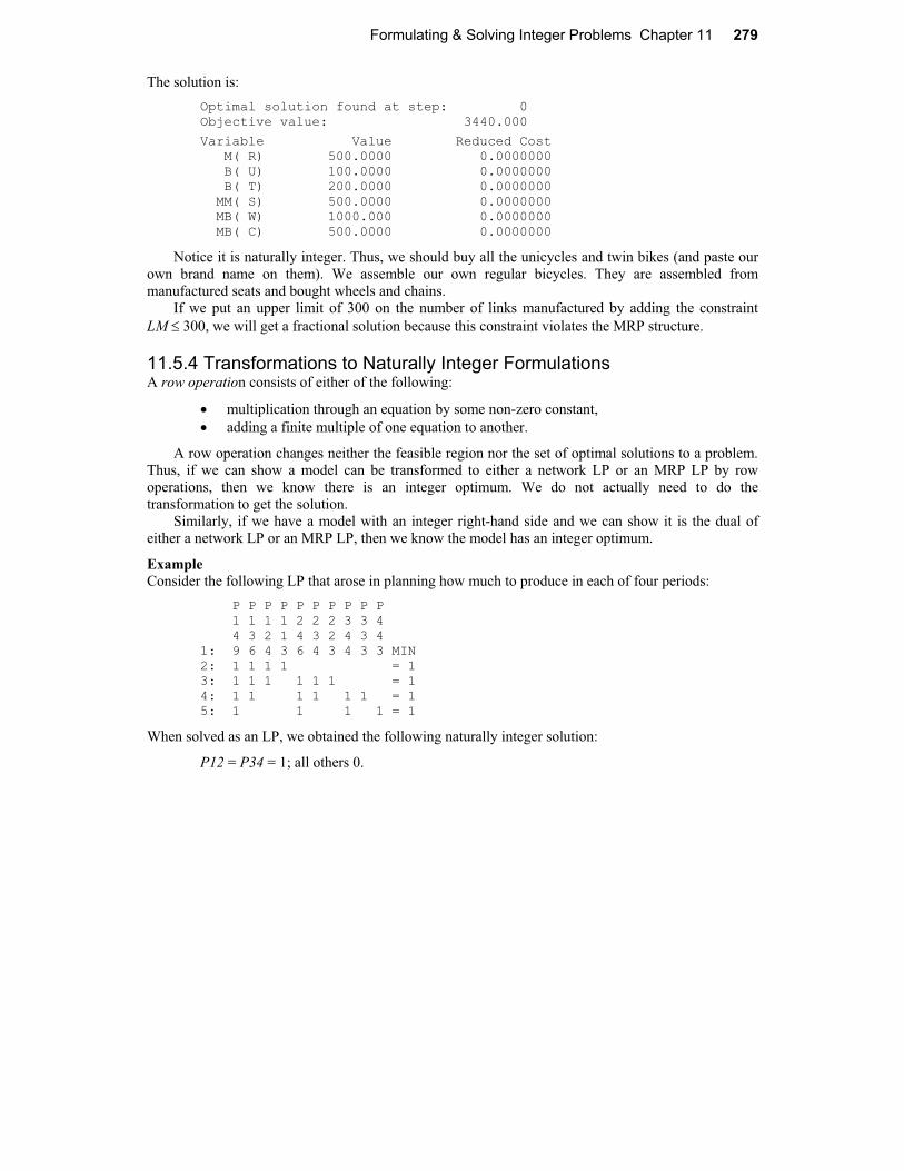
The solution is:
Optimal solution found at step: 0 Objective value: 3440.000
Variable Value Reduced Cost M( R) 500.0000 0.0000000 B( U) 100.0000 0.0000000 B( T) 200.0000 0.0000000 MM( S) 500.0000 0.0000000 MB( W) 1000.000 0.0000000 MB( C) 500.0000 0.0000000
Notice it is naturally integer. Thus, we should buy all the unicycles and twin bikes (and paste our own brand name on them). We assemble our own regular bicycles. They are assembled from manufactured seats and bought wheels and chains. If we put an upper limit of 300 on the number of links manufactured by adding the constraint
LM 300, we will get a fractional solution because this constraint violates the MRP structure.
11.5.4 Transformations to Naturally Integer Formulations A row operation consists of either of the following:
multiplication through an equation by some non-zero constant,
adding a finite multiple of one equation to another.
A row operation changes neither the feasible region nor the set of optimal solutions to a problem. Thus, if we can show a model can be transformed to either a network LP or an MRP LP by row operations, then we know there is an integer optimum. We do not actually need to do the transformation to get the solution. Similarly, if we have a model with an integer right-hand side and we can show it is the dual of either a network LP or an MRP LP, then we know the model has an integer optimum.
Example
Consider the following LP that arose in planning how much to produce in each of four periods:
P P P P P P P P P P 1 1 1 1 2 2 2 3 3 4 4 3 2 1 4 3 2 4 3 4 1: 9 6 4 3 6 4 3 4 3 3 MIN 2: 1 1 1 1 = 1 3: 1 1 1 1 1 1 = 1 4: 1 1 1 1 1 1 = 1 5: 1 1 1 1 = 1
When solved as an LP, we obtained the following naturally integer solution:
P12 = P34 = 1; all others 0.

280 Chapter 11 Formulating & Solving Integer Programs
Could we have predicted a naturally integer solution beforehand? If we perform the row
operations: (5') = (5) (4); (4') = (4) (3); (3') = (3) (2), we obtain the equivalent LP:
P P P P P P P P P P 1 1 1 1 2 2 2 3 3 4 4 3 2 1 4 3 2 4 3 4 1: 9 6 4 3 6 4 3 4 3 3 MIN 2: 1 1 1 1 = 1 3': -1 1 1 1 = 0 4': -1 -1 1 1 = 0 5': -1 -1 -1 1 = 0
This is a network LP, so it has a naturally integer solution.
Example
In trying to find the minimum elapsed time for a certain project composed of seven activities, the following LP was constructed (in PICTURE form):
A B C D E F 1:-1 ' 1 MIN AB:-1 1 ' >= 3 AC:-1 '1 ' ' >= 2 BD: -1 1 >= 5 BE: -1 ' 1 >= 6 CF: ' -1 ' '1 >= 4 DF: -1 1 >= 7 EF: '-1 1 >= 6
This is neither a network LP (e.g., consider columns A, B, or F) nor an MRP LP (e.g., consider columns A or F). Nevertheless, when solved, we get the naturally integer solution:
Optimal solution found at step: 0 Objective value: 15.00000
Variable Value Reduced Cost A 0.0000000 0.0000000 B 3.000000 0.0000000 C 2.000000 0.0000000 D 8.000000 0.0000000 E 9.000000 0.0000000 F 15.00000 0.0000000
Row Slack or Surplus Dual Price 1 15.00000 1.000000 AB 0.0000000 -1.000000 AC 0.0000000 0.0000000 BD 0.0000000 -1.000000 BE 0.0000000 0.0000000 CF 9.000000 0.0000000 DF 0.0000000 -1.000000 EF 0.0000000 0.0000000
Could we have predicted a naturally integer solution beforehand? If we look at the PICTURE of
the model, we see each constraint has exactly one +1 and one 1. Thus, its dual model is a network LP and expectation of integer answers is justified.

Formulating & Solving Integer Problems Chapter 11 281
11.6 The Assignment Problem and Related Sequencing and Routing Problems
The assignment problem is a simple LP problem, which is frequently encountered as a major component in more complicated practical problems. The assignment problem is:
Given a matrix of costs: cij = cost of assigning object i to person j,
and variables: xij = 1 if object i is assigned to person j.
Then, we want to:
Minimize ji cijxij
subject to
i xij = 1 for each object i,
j xij = 1 for each person i,
xij > 0.
This problem is easy to solve as an LP and the xij will be naturally integer. There are a number of problems in routing and sequencing that are closely related to the assignment problem.
11.6.1 Example: The Assignment Problem Large airlines tend to base their route structure around the hub concept. An airline will try to have a large number of flights arrive at the hub airport during a certain short interval of time (e.g., 9 A.M. to 10 A.M.) and then have a large number of flights depart the hub shortly thereafter (e.g., 10 A.M. to 11 A.M.). This allows customers of that airline to travel between a large combination of origin/destinationcities with one stop and at most one change of planes. For example, United Airlines uses Chicago as a hub, Delta Airlines uses Atlanta, and American uses Dallas/Fort Worth. A desirable goal in using a hub structure is to minimize the amount of changing of planes (and the resulting moving of baggage) at the hub. The following little example illustrates how the assignment model applies to this problem. A certain airline has six flights arriving at O’Hare airport between 9:00 and 9:30 A.M. The same six airplanes depart on different flights between 9:40 and 10:20 A.M. The average numbers of people transferring between incoming and leaving flights appear below:
L01 L02 L03 L04 L05 L06
I01 20 15 16 5 4 7
I02 17 15 33 12 8 6
I03 9 12 18 16 30 13
I04 12 8 11 27 19 14 Flight I05 arrives too late to
I05 0 7 10 21 10 32 connect with L01. Similarly I06 is
I06 0 0 0 6 11 13 too late for flights L01, L02, and L03.

282 Chapter 11 Formulating & Solving Integer Programs
All the planes are identical. A decision problem is which incoming flight should be assigned to which outgoing flight. For example, if incoming flight I02 is assigned to leaving flight L03, then 33 people (and their baggage) will be able to remain on their plane at the stop at O’Hare. How should incoming flights be assigned to leaving flights, so a minimum number of people need to change planes at the O’Hare stop? This problem can be formulated as an assignment problem if we define:
xij = 1 if incoming flight i is assigned to outgoing flight j,
0 otherwise.
The objective is to maximize the number of people not having to change planes. A formulation is:
MODEL: ! Assignment model(ASSIGNMX); SETS: FLIGHT; ASSIGN( FLIGHT, FLIGHT): X, CHANGE; ENDSETSDATA: FLIGHT = 1..6; ! The value of assigning i to j; CHANGE = 20 15 16 5 4 7 17 15 33 12 8 6 9 12 18 16 30 13 12 8 11 27 19 14 -999 7 10 21 10 32 -999 -999 -999 6 11 13; ENDDATA!---------------------------------;! Maximize value of assignments; MAX = @SUM(ASSIGN: X * CHANGE); @FOR( FLIGHT( I): ! Each I must be assigned to some J; @SUM( FLIGHT( J): X( I, J)) = 1; ! Each I must receive an assignment; @SUM( FLIGHT( J): X( J, I)) = 1; ); END
Notice, we have made the connections that are impossible prohibitively unattractive. A solution is:
Optimal solution found at step: 9 Objective value: 135.0000
Variable Value Reduced Cost X( 1, 1) 1.000000 0.0000000 X( 2, 3) 1.000000 0.0000000 X( 3, 2) 1.000000 0.0000000 X( 4, 4) 1.000000 0.0000000 X( 5, 6) 1.000000 0.0000000 X( 6, 5) 1.000000 0.0000000
Notice, each incoming flight except I03 is able to be assigned to its most attractive outgoing flight. The solution is naturally integer even though we did not declare any of the variables to be integer.

Formulating & Solving Integer Problems Chapter 11 283
11.6.2 The Traveling Salesperson Problem One of the more famous optimization problems is the traveling salesperson problem (TSP). It is an assignment problem with the additional condition that the assignments chosen must constitute a tour. The objective is to minimize the total distance traveled. Lawler et al. (1985) presents a tour-de-force on this fascinating problem. One example of a TSP occurs in the manufacture of electronic circuit boards. Danusaputro, Lee, and Martin-Vega (1990) discuss the problem of how to optimally sequence the drilling of holes in a circuit board, so the total time spent moving the drill head between holes is minimized. A similar TSP occurs in circuit board manufacturing in determining the sequence in which components should be inserted onto the board by an automatic insertion machine. Another example is the sequencing of cars on a production line for painting: each time there is a change in color, a setup cost and time is incurred. A TSP is described by the data: cij = cost of traveling directly from city i to city j, e.g., the distance. A solution is described by the variables: yij = 1 if we travel directly from i to j, else 0. The objective is:
Min i j cij yij ;
We will describe several different ways of specifying the constraints.
Subtour Elimination Formulation: (1) We must enter each city j exactly once:
i jn yij = 1 for j = 1 to n,
(2) We must exit each city i exactly once:
j in yij = 1 for i = 1 to n,
(3) yij = 0 or 1, for i = 1, 2, …, n, j = 1, 2, …, n, i j:
(4) No subtours are allowed for any subset of cities S not including city 1:
i j S,
yij < |S| 1 for every subset S,
where |S| is the size of S.
The above formulation is usually attributed to Dantzig, Fulkerson, and Johnson(1954). An unattractive feature of the Subtour Elimination formulation is that if there are n cities, then there are approximately 2n constraints.
Cumulative Load Formulation:
We can reduce the number of constraints substantially if we define: uj = the sequence number of city j on the trip. Equivalently, if each city requires one unit of something to be picked up(or delivered), then uj = cumulative number of units picked up(or delivered) after the stop at j. We replace constraint set (4) by:

284 Chapter 11 Formulating & Solving Integer Programs
(5) uj > ui + 1 (1 yij)n for i = 1, 2, ..., j = 2, 3, 4, . . . ; j i.
The approach of constraint set (5) is due to Miller, Tucker, and Zemlin(1960). There are only approximately n2 constraints of type (5), however, constraint set (4) is much tighter than (5). Large problems may be computationally intractable if (4) is not used. Even though there are a huge number of constraints in (4), only a few of them may be binding at the optimum. Thus, an iterative approach that adds violated constraints of type (4) as needed works surprisingly well. Padberg and Rinaldi (1987) used essentially this iterative approach and were able to solve to optimality problems with over 2000 cities. The solution time was several hours on a large computer.
Multi-commodity Flow Formulation:
Similar to the previous formulation, imagine that each city needs one unit of some commodity distinct to that city. Define:
xijk = units of commodity carried from i to j, destined for ultimate delivery to k.
If we assume that we start at city 1 and there are n cities, then we replace constraint set (4) by:
For k = 1, 2, 3, …, n:
j >1 x1jk = 1; ( Each unit must be shipped out of the origin.)
i k xikk = 1; ( Each city k must get its unit.)
For j = 2, 3, …, n, k =1, 2, 3, …, n, j k:
i xijk = t j xjtk ( Units entering j, but not destined for j, must depart j to some city t.)
A unit cannot return to 1, except if its final destination is 1:
i k > 1 xi1k = 0,
For i = 1, 2, …, n, j = 1, 2, …, n, k = 1, 2, …, n, i j:
xijk yij ( If anything shipped from i to j, then turn on yij.)
The drawback of this formulation is that it has approximately n3 constraints and variables. A remarkable feature of the multicommodity flow formulation is that it is just as tight as the Subtour Elimination formulation. The multi-commodity formulation is due to Claus(1984).
Heuristics For practical problems, it may be important to get good, but not necessarily optimal, answers in just a few seconds or minutes rather than hours. The most commonly used heuristic for the TSP is due to Lin and Kernighan (1973). This heuristic tries to improve a given solution by clever re-orderings of cities in the tour. For practical problems (e.g., in operation sequencing on computer controlled machines), the heuristic seems always to find solutions no more than 2% more costly than the optimum. Bland and Shallcross (1989) describe problems with up to 14,464 “cities” arising from the sequencing of operations on a computer controlled machine. In no case was the Lin-Kernighan heuristic more than 1.7% from the optimal for these problems.
Formulating & Solving Integer Problems Chapter 11 285
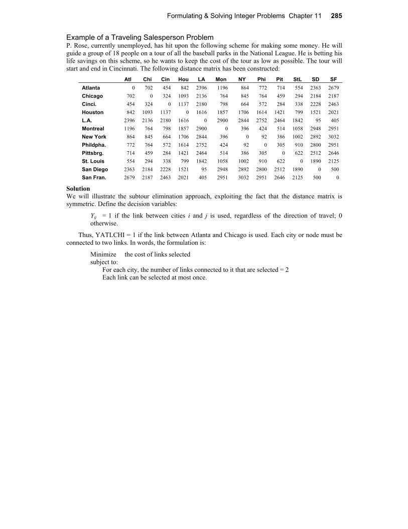
Example of a Traveling Salesperson Problem P. Rose, currently unemployed, has hit upon the following scheme for making some money. He will guide a group of 18 people on a tour of all the baseball parks in the National League. He is betting his life savings on this scheme, so he wants to keep the cost of the tour as low as possible. The tour will start and end in Cincinnati. The following distance matrix has been constructed:
Atl Chi Cin Hou LA Mon NY Phi Pit StL SD SF
Atlanta 0 702 454 842 2396 1196 864 772 714 554 2363 2679
Chicago 702 0 324 1093 2136 764 845 764 459 294 2184 2187
Cinci. 454 324 0 1137 2180 798 664 572 284 338 2228 2463
Houston 842 1093 1137 0 1616 1857 1706 1614 1421 799 1521 2021
L.A. 2396 2136 2180 1616 0 2900 2844 2752 2464 1842 95 405
Montreal 1196 764 798 1857 2900 0 396 424 514 1058 2948 2951
New York 864 845 664 1706 2844 396 0 92 386 1002 2892 3032
Phildpha. 772 764 572 1614 2752 424 92 0 305 910 2800 2951
Pittsbrg. 714 459 284 1421 2464 514 386 305 0 622 2512 2646
St. Louis 554 294 338 799 1842 1058 1002 910 622 0 1890 2125
San Diego 2363 2184 2228 1521 95 2948 2892 2800 2512 1890 0 500
San Fran. 2679 2187 2463 2021 405 2951 3032 2951 2646 2125 500 0
Solution
We will illustrate the subtour elimination approach, exploiting the fact that the distance matrix is symmetric. Define the decision variables:
Yij = 1 if the link between cities i and j is used, regardless of the direction of travel; 0 otherwise.
Thus, YATLCHI = 1 if the link between Atlanta and Chicago is used. Each city or node must be connected to two links. In words, the formulation is:
Minimize the cost of links selected subject to:
For each city, the number of links connected to it that are selected = 2 Each link can be selected at most once.

286 Chapter 11 Formulating & Solving Integer Programs
The LINGO formulation is shown below:
MODEL:SETS:CITY;ROUTE(CITY, CITY)|&1 #GT# &2:COST, Y;
ENDSETSDATA: CITY= ATL CHI CIN HOU LA MON NY PHI PIT STL SD SF; COST= 702 454 324 842 1093 1137 2396 2136 2180 1616 1196 764 798 1857 2900 864 845 664 1706 2844 396 772 764 572 1614 2752 424 92 714 459 284 1421 2464 514 386 305 554 294 338 799 1842 1058 1002 910 622 2363 2184 2228 1521 95 2948 2892 2800 2512 1890 2679 2187 2463 2021 405 2951 3032 2951 2646 2125 500;
ENDDATAMIN = @SUM( ROUTE: Y * COST); @SUM( CITY( I)|I #GE# 2: Y(I, 1)) = 2; @FOR( CITY( J)|J #GE# 2: @SUM(CITY(I)| I #GT# J: Y(I, J)) + @SUM(CITY(K)|K #LT# J: Y(J, K))=2); @FOR( ROUTE: Y <= 1);
END
When this model is solved as an LP, we get the solution:
Optimal solution found at step: 105 Objective value: 5020.000
Variable Value Reduced Cost Y( CIN, ATL) 1.000000 0.0000000 Y( CIN, CHI) 1.000000 0.0000000 Y( HOU, ATL) 1.000000 0.0000000 Y( NY, MON) 1.000000 0.0000000 Y( PHI, NY) 1.000000 0.0000000 Y( PIT, MON) 1.000000 0.0000000 Y( PIT, PHI) 1.000000 0.0000000 Y( STL, CHI) 1.000000 0.0000000 Y( STL, HOU) 1.000000 0.0000000 Y( SD, LA) 1.000000 0.0000000 Y( SF, LA) 1.000000 0.0000000 Y( SF, SD) 1.000000 0.0000000
This has a cost of 5020 miles. Graphically, it corresponds to Figure 11.6.

Formulating & Solving Integer Problems Chapter 11 287
Figure 11.6
SNF
LAX
SND
HOU
ATL
STL
CHI
MON
CIN
PIT PHI
NYK
Unfortunately, the solution has three subtours. We can cut off the smallest subtour by adding the constraint:
!SUBTOUR ELIMINATION; Y( SF, LA) + Y( SD, LA) + Y( SF, SD) <= 2;
Now, when we solve it as an LP, we get a solution with cost 6975, corresponding to Figure 11.7:
Figure 11.7
SNF
LAX
SND
HOU
ATL
STL
CHI
MON
CIN
PIT PHI
NYK

288 Chapter 11 Formulating & Solving Integer Programs
We cut off the subtour in the southwest by appending the constraint:
Y(LA, HOU) + Y(SD, HOU) + Y(SF, LA) + Y(SF, SD)<= 3;
We continue in this fashion appending subtour elimination cuts:
Y(CIN,ATL) + Y(CIN,ATL) + Y(CIN,CHI) + Y(HOU,ATL) + Y(STL,CHI) + Y(STL,HOU) <= 4;
Y(NY,MON) + Y(PHI,NY) + Y(PIT,MON) + Y(PIT,PHI) <= 3; Y(SD,LA) + Y(SF,LA) + Y(SF,SD) <= 2; Y(NY,MON) + Y(PHI,MON) + Y(PHI,NY) <= 2; Y(CIN,ATL) + Y(PIT,CHI) + Y(PIT,CIN) + Y(STL,ATL) + Y(STL,CHI) <= 4; Y(SD,HOU) + Y(SD,LA) + Y(SF,HOU) + Y(SF,LA) <= 3; Y(CIN,ATL) + Y(CIN,CHI) + Y(STL,ATL) + Y(STL,CHI) <= 3; Y(PHI,MON) + Y(PHI,NY) + Y(PIT,MON) + Y(PIT,NY) <= 3; Y(CIN,ATL) + Y(MON,CHI) + Y(NY,MON) + Y(PHI,NY) + Y(PIT,CIN) + PIT,PHI) + Y(STL,ATL) + Y(STL,CHI) <= 7;
Y(SD,LA) + Y(SF,HOU) + Y(SF,SD) + Y(LA,HOU) <= 3;
After the above are all appended, we get the solution shown in Figure 11.8. It is a complete tour with cost $7,577.
Figure 11.8
SNF
LAX
SND
HOU
ATL
STL
CHI
MON
CIN
PIT PHI
NYK
Note only LPs were solved. No branch-and-bound was required, although in general branching may be required. Could P. Rose have done as well by trial and error? The most obvious heuristic is the “closest unvisited city” heuristic. If one starts in Cincinnati and next goes to the closest unvisited city at each step and finally returns to Cincinnati, the total distance is 8015 miles, about 6% worse than the optimum.

Formulating & Solving Integer Problems Chapter 11 289
The Optional Stop TSP
If we drop the requirement that every stop must be visited, we then get the optional stop TSP. This might correspond to a job sequencing problem where vj is the profit from job j if we do it and cij is the cost of switching from job i to job j. Let:
yj = 1 if city j is visited, 0 otherwise.
If vj is the value of visiting city j, then the objective is:
Minimize i j
cij xij vj yj .
The constraint sets are:
(1) Each city j can be visited at most once
i jxij = yj
(2) If we enter city j, then we must exit it:
k jxjk = yj
(3) No subtours allowed for each subset, S, of cities not including the home base 1.
i j S,xij < |S| 1, where |S| is the size of S.
For example, if there are n cities, including the home base, then there are
(n 1) (n 2)/(3 2) subsets of size 3.
(4) Alternatively, (3) may be replaced by
uj > ui + 1 (1 xij)n for j = 2, 3, . . . , n.
Effectively, uj is the sequence number of city j in its tour. Constraint set (3) is much tighter than (4).
11.6.3 Capacitated Multiple TSP/Vehicle Routing Problems An important practical problem is the routing of vehicles from a central depot. An example is the routing of delivery trucks for a metropolitan newspaper. You can think of this as a multiple traveling salesperson problem with finite capacity for each salesperson. This problem is sometimes called the LTL(Less than TruckLoad) routing problem because a typical recipient receives less than a truck load of goods. A formulation is: Given:
V = capacity of a vehicle dj = demand of city or stop j
Each city, j, must be visited once for j > 1:
jxij = 1

290 Chapter 11 Formulating & Solving Integer Programs
Each city i > 1, must be exited once:
i
xij = 1
No subtours:
i j s,xij < |S| 1,
No overloads: For each set of cities T, including 1, which constitute more than a truckload:
i j T,xij < |T| k,
where k = minimum number of cities that must be dropped from T to reduce it to one load.
This formulation can solve to optimality modest-sized problems of say, 25 cities. For larger or more complicated practical problems, the heuristic method of Clarke and Wright (1964) is a standard starting point for quickly finding good, but not necessarily optimal, solutions. The following is a generic LINGO model for vehicle routing problems:
MODEL: ! (VROUTE); ! The Vehicle Routing Problem (VRP) occurs in many servicesystems such as delivery, customer pick-up, repair andmaintenance. A fleet of vehicles, each with fixedcapacity, starts at a common depot and returns to thedepot after visiting locations where service is demanded. Problems with more than a dozen cities can take lots of time.
This instance involves delivering the required amount of goods to 9 cities from a depot at city 1;
SETS:CITY/ Chi Den Frsn Hous KC LA Oakl Anah Peor Phnx/: Q, U; ! Q(I) = amount required at city I(given),
must be delivered by just 1 vehicle. U(I) = accumulated deliveries at city I ;
CXC( CITY, CITY): DIST, X; ! DIST(I,J) = distance from city I to city J
X(I,J) is 0-1 variable,= 1 if some vehicle travels from city I to J, else 0 ;
ENDSETSDATA:! city 1 represents the common depot, i.e. Q( 1) = 0;
Q= 0 6 3 7 7 18 4 5 2 6;

Formulating & Solving Integer Problems Chapter 11 291
! distance from city I to city J is same from J to I, distance from city I to the depot is 0, because vehicle need not return to the depot ; DIST= ! To City; !Chi Den Frsn Hous KC LA Oakl Anah Peor Phnx From;
0 996 2162 1067 499 2054 2134 2050 151 1713! Chicago; 0 0 1167 1019 596 1059 1227 1055 904 792! Denver; 0 1167 0 1747 1723 214 168 250 2070 598! Fresno; 0 1019 1747 0 710 1538 1904 1528 948 1149! Houston; 0 596 1723 710 0 1589 1827 1579 354 1214! K. City; 0 1059 214 1538 1589 0 371 36 1943 389! L. A.; 0 1227 168 1904 1827 371 0 407 2043 755! Oakland; 0 1055 250 1528 1579 36 407 0 1933 379! Anaheim; 0 904 2070 948 354 1943 2043 1933 0 1568! Peoria; 0 792 598 1149 1214 389 755 379 1568 0;! Phoenix;
! VCAP is the capacity of a vehicle ; VCAP = 18;
ENDDATA!----------------------------------------------------------;! The objective is to minimize total travel distance; MIN = @SUM( CXC: DIST * X);
! for each city, except depot....; @FOR( CITY( K)| K #GT# 1:
! a vehicle does not travel inside itself,...; X( K, K) = 0;
! a vehicle must enter it,... ; @SUM( CITY( I)| I #NE# K #AND# ( I #EQ# 1 #OR# Q( I) + Q( K) #LE# VCAP): X( I, K)) = 1; ! a vehicle must leave it after service ;
@SUM( CITY( J)| J #NE# K #AND# ( J #EQ# 1 #OR# Q( J) + Q( K) #LE# VCAP): X( K, J)) = 1;
! U( K) = amount delivered on trip up to city K >= amount needed at K but <= vehicle capacity; @BND( Q( K), U( K), VCAP);
! If K follows I, then can bound U( K) - U( I); @FOR( CITY( I)| I #NE# K #AND# I #NE# 1: U( K) >= U( I) + Q( K) - VCAP + VCAP*( X( K, I) + X( I, K)) - ( Q( K) + Q( I)) * X( K, I);
);
! If K is 1st stop, then U( K) = Q( K); U( K) <= VCAP - ( VCAP - Q( K)) * X( 1, K); ! If K is not 1st stop...; U( K) >=Q( K)+ @SUM( CITY( I)| I #GT# 1: Q( I) * X( I, K)); );
! Make the X's binary; @FOR( CXC( I, J): @BIN( X( I, J)) ;);
! Must send enough vehicles out of depot; @SUM( CITY( J)| J #GT# 1: X( 1, J)) >=@FLOOR((@SUM( CITY( I)| I #GT# 1: Q( I))/ VCAP) + .999);
END

292 Chapter 11 Formulating & Solving Integer Programs
Optimal solution found at step: 973 Objective value: 6732.000
Variable Value X( CHI, HOUS) 1.000000 X( CHI, LA) 1.000000 X( CHI, PEOR) 1.000000 X( CHI, PHNX) 1.000000 X( DEN, CHI) 1.000000 X( FRSN, OAKL) 1.000000 X( HOUS, CHI) 1.000000 X( KC, DEN) 1.000000 X( LA, CHI) 1.000000 X( OAKL, CHI) 1.000000 X( ANAH, FRSN) 1.000000 X( PEOR, KC) 1.000000 X( PHNX, ANAH) 1.000000
By following the links, you can observe that the trips are:
Chicago - Houston; Chicago - LA; Chicago - Peoria - KC - Denver; Chicago - Phoenix - Anaheim - Fresno - Oakland.
Combined DC Location/Vehicle Routing
Frequently, there is a vehicle routing problem associated with opening a new plant or distribution center (DC). Specifically, given the customers to be served from the DC, what trips are made, so as to serve the customers at minimum cost. A “complete” solution to the problem would solve the location and routing problems simultaneously. The following IP formulation illustrates one approach:
Parameters
Fi = fixed cost of having a DC at location i,Cj = cost of using route j,aijk = 1 if route j originates at DC i and serves customer k. There is exactly one DC
associated with each route.
Decision variables
yi = 1 if we use DC i, else 0, xj = 1 if we use route j, else 0
The Model
Minimize i
Fi yi + j
cj xj
subject to (Demand constraints) For each customer k:
jiaijk xj = 1
(Forcing constraints) For each DC i and customer k:
jaijk xj yi

Formulating & Solving Integer Problems Chapter 11 293
11.6.4 Minimum Spanning TreeA spanning tree of n nodes is a collection of n 1 arcs, so there is exactly one path between every pair of nodes. A minimum cost spanning tree might be of interest, for example, in designing a communications network. Assume node 1 is the root of the tree. Let xij = 1 if the path from 1 to j goes through node iimmediately before node j, else xij = 0. A formulation is:
Minimize i j
cijxij
subject to
(1)ji
xij = n 1,
(2) i j S,
xij < |S| 1 for every strict subset S of {1, 2,…,n},
xij = 0 or 1.
An alternative to (1) and (2) is the following set of constraints based on assigning a unique sequence number uj to each node:
1,ij
i j
x for j = 2, 3, 4,…,n,
uj > ui + xij (n –2) (1 xij)+(n-3)xji, for j = 2, 3, 4, . . . , n.uj > 0.
In this case, uj is the number of arcs between node j and node 1. A numeric example of the sequence numbering formulation is in section 8.9.8. If one has a pure spanning tree problem, then the “greedy” algorithm of Kruskal (1956) is a fast way of finding optimal solutions.
11.6.5 The Linear Ordering Problem A problem superficially similar to the TSP is the linear ordering problem. One wants to find a strict ordering of n objects. Applications are to ranking in sports tournaments, product preference ordering in marketing, job sequencing on one machine, ordering of industries in an input-output matrix, ordering of historical objects in archeology, and others. See Grötschel et al. (1985) for a further discussion. The linear ordering problem is similar to the approach of conjoint analysis sometimes used in marketing. The crucial input data are cost entries cij. If object i appears anywhere before object j in the proposed ordering, then cij is the resulting cost. The decision variables are:
xij = 1 if object i precedes object j, either directly or indirectly for all i j.
The problem is:
Minimize ji
cij xij
subject to
(1) xij + xji = 1 for all i j
294 Chapter 11 Formulating & Solving Integer Programs
If i precedes j and j precedes k, then we want to imply that i precedes k. This is enforced with the constraints:
(2) xij + xjk + xki < 2 for all i, j, k with i j, i k, j k.
The size of the formulation can be cut in two by noting that xij = 1 xji. Thus, we substitute out xji
for j > i. Constraint set (1) becomes simply 0 < xij < 1. Constraint set (2) becomes:
(2') xij + xjk xik + sijk = 1 for all i < j < k0 < sijk < 1
There are n!/((n 3)! 3!) = n (n 1) (n 2)/6 ways of choosing 3 objects from n, so the number of constraints is approximately n3/6.
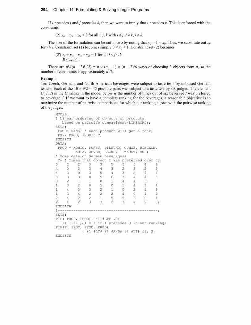
ExampleTen Czech, German, and North American beverages were subject to taste tests by unbiased German
testers. Each of the 10 9/2 = 45 possible pairs was subject to a taste test by six judges. The element C( I, J) in the C matrix in the model below is the number of times out of six beverage I was preferred to beverage J. If we want to have a complete ranking for the beverages, a reasonable objective is to maximize the number of pairwise comparisons for which our ranking agrees with the pairwise ranking of the judges:
MODEL:! Linear ordering of objects or products, based on pairwise comparisons(LINERORD);SETS: PROD: RANK; ! Each product will get a rank; PXP( PROD, PROD): C; ENDSETSDATA: PROD = KONIG, FURST, PILSURQ, GUNZB, RIEGELE, PAULA, JEVER, BECKS, WARST, BUD; ! Some data on German beverages; C= ! Times that object I was preferred over J; 0 2 2 3 3 5 5 5 4 4 4 0 3 3 4 3 2 3 2 2 4 3 0 3 5 4 3 2 4 4 3 3 3 0 5 6 3 4 4 3 3 2 1 1 0 1 4 4 5 3 1 3 2 0 5 0 5 4 1 4 1 4 3 3 2 1 0 2 1 3 1 3 4 2 2 2 4 0 4 2 2 4 2 2 1 5 5 2 0 4 2 4 2 3 3 2 3 4 2 0; ENDDATA!---------------------------------------------;SETS:PIP( PROD, PROD)| &1 #LT# &2: X; ! X(I,J) = 1 if I precedes J in our ranking;PIPIP( PROD, PROD, PROD) | &1 #LT# &2 #AND# &2 #LT# &3: S; ENDSETS

Formulating & Solving Integer Problems Chapter 11 295
! Maximize the number of times our pairwise ordering matches that of our testers; MAX = @SUM( PIP( I, J): C( I, J) * X( I, J) + C( J, I) *(1 - X( I, J))); ! The rankings must be transitive, that is, If I->J and J->K, then I->K; @FOR( PIPIP( I, J, K):! Note N*(N-1)*(N-2)/6 of these!; X( I, J) + X ( J, K) - X( I, K) + S( I, J, K) = 1; @BND( 0, S( I, J, K), 1); ); @FOR( PIP: @BIN( X);); ! Make X's 0 or 1;
! Count number products before product I( + 1); @FOR( PROD( I): RANK( I) = 1 + @SUM( PIP( K, I): X( K, I)) + @SUM( PIP( I, K): 1 - X( I, K)); );END
When solved, we get an optimal objective value of 168. This means out of the (10 * 9/2)* 6 = 270 pairwise comparisons, the pairwise rankings agreed with LINGO's complete ranking 168 times:
Optimal solution found at step: 50 Objective value: 168.0000 Branch count: 0
Variable Value Reduced Cost RANK( KONIG) 3.000000 0.0000000 RANK( FURST) 10.00000 0.0000000 RANK( PILSURQ) 2.000000 0.0000000 RANK( GUNZB) 1.000000 0.0000000 RANK( RIEGELE) 7.000000 0.0000000 RANK( PAULA) 5.000000 0.0000000 RANK( JEVER) 9.000000 0.0000000 RANK( BECKS) 8.000000 0.0000000 RANK( WARST) 4.000000 0.0000000 RANK( BUD) 6.000000 0.0000000
According to this ranking, GUNZB comes out number 1 (most preferred), while FURST comes out tenth (least preferred). It is important to note that there may be alternate optima. This means there may be alternate orderings, all of which match the input pairings 168 times out of 270. In fact, you can show that there is another ordering with a value of 168 in which PILSURQ is ranked first.

296 Chapter 11 Formulating & Solving Integer Programs
11.6.6 Quadratic Assignment Problem The quadratic assignment problem has the same constraint set as the linear assignment problem. However, the objective function contains products of two variables. Notationally, it is:
Min lkji
ci j k l xi j xk l
subject to: For each j:
i
xi j = 1
For each i:
jxi j = 1
Some examples of this problem are:
(a) Facility layout. If djl is the physical distance between room j and room l; sik is the communication traffic between department i and k; and xij = 1 if department i is assigned to room j, then we want to minimize:
lkjixij xkl djl sik
(b) Vehicle to gate assignment at a terminal. If djl is the distance between gate j and gate l at an airline terminal, passenger train station, or at a truck terminal; sik is the number of passengers or tons of cargo that needs to be transferred between vehicle i and vehicle k; and xij = 1 if vehicle i (incoming or outgoing) is assigned to gate j, then we again want to minimize:
lkjixij xkl djl sik
(c) Radio frequency assignment. If dij is the physical distance between transmitters i and j; skl
is the distance in frequency between k and l; and pi is the power of transmitter I, then we want max{pi, pj} (1/dij)(1/skl) to be small if transmitter i is assigned frequency k and transmitter j is assigned frequency l.
(d) VLSI chip layout. The initial step in the design of a VLSI (very large scale integrated) chip is typically to assign various required components to various areas on the chip. See Sarrafzadeh and Wong (1996) for additional details. Steinberg (1961) describes the case of assigning electronic components to a circuit board, so as to minimize the total interconnection wire length. For the chip design case, typically the chip area is partitioned into 2 to 6 areas. If djl is the physical distance between area j and area l; sik is the number of connections required between components i and k; and xij = 1 if component i is assigned to area j, then we again want to minimize:
lkjixij xkl djl sik
(e) Disk file allocation. If wij is the interference if files i and j are assigned to the same disk, we want to assign files to disks, so total interference is minimized.

Formulating & Solving Integer Problems Chapter 11 297
(f) Type wheel design. Arrange letters and numbers on a type wheel, so (a) most frequently used ones appear together and (b) characters that tend to get typed together (e.g., q u) appear close together on the wheel.
The quadratic assignment problem is a notoriously difficult problem. If someone asks you to solve such a problem, you should make every effort to show the problem is not really a quadratic assignment problem. One indication of its difficulty is the solution is not naturally integer. One of the first descriptions of quadratic assignment problems was by Koopmans and Beckmann (1957). For this reason, this problem is sometimes known as the Koopmans-Beckmann problem. They illustrated the use of this model to locate interacting facilities in a large country. Elshafei (1977) illustrates the use of this model to lay out a hospital. Specifically, 19 departments are assigned to 19 different physical regions in the hospital. The objective of Elshafei was to minimize the total distance patients had to walk between departments. The original assignment used in the hospital required a distance of 13,973,298 meters per year. An optimal assignment required a total distance of 8,606,274 meters. This is a reduction in patient travel of over 38%. Small quadratic assignment problems can be converted to linear integer programs by the transformation:
Replace the product xij xkl by the single variable zijkl. The objective is then:
Min lkji
ci j k l zi jk l
Notice if there are N departments and N locations, then there are N N variables of type xij, and
N N N N variables of type zijkl variables. This formulation can get large quickly. Several reductions are possible:
1) The terms cijkl xij xkl and c klij xkl xij can be combined into the term:
(cijkl + c klij ) xkl xij
to reduce the number of z variables and associated constraints needed by a factor of 2.
2) Certain assignments can be eliminated beforehand (e.g., a large facility to a small location). Many of the cross terms, cijkl , are zero (e.g., if there is no traffic between facility i and facility k), so the associated z variables need not be introduced.
The non-obvious thing to do now is to ensure that zijkl = 1 if and only if both xij and xkl = 1. Sherali and Adams(1999) point out that constraints of the following type will enforce this requirement: For a given i, k, l:
,
kl ijkl
j j l
x z
In words, if object k is assigned to location l, then for any other object i, i k, there must be some
other location j, j l, to which i is assigned.

298 Chapter 11 Formulating & Solving Integer Programs
The following is a LINGO implementation of the above for deciding which planes should be assigned to which gates at an airport, so that the distance weighted cost of changing planes for the passengers is minimized:
MODEL:! Quadratic assignment problem(QAP006); ! Given number of transfers between flights, distance between gates, assign flights to gates to minimize total transfer cost; SETS: FLIGHT/1..6/; GATE/ E3 E4 E5 F3 F4 F5/;! Gates at terminal 2 of O'Hare; GXG( GATE, GATE)| &1 #LT# &2: T; ! Inter gate times(symmetric); FXF( FLIGHT, FLIGHT)| &1 #LT# &2: N; ! Transfers between flights; FXG( FLIGHT, GATE): X; ! Flight to gate assignment variable; ENDSETS DATA: T = 70 40 60 90 90 ! Time between gates; 50 100 80 110 100 90 130 60 40 30; N = 12 0 12 0 5 30 35 20 13 ! No. units between flights; 40 20 10 0 6 14; ENDDATA !--------------------------------------------------------;! Warning: may be very slow for no. objects > 7; SETS: ! Warning: this set gets big fast!; TGTG( FLIGHT, GATE, FLIGHT, GATE)| &1 #LT# &3: Z; ENDSETS
! Min the cost of transfers * distance; MIN = @SUM( TGTG( B, J, C, K)| J #LT# K: Z( B, J, C, K) * N( B, C) * T( J, K)) + @SUM( TGTG( B, J, C, K)| J #GT# K: Z( B, J, C, K) * N( B, C) * T( K, J)); ! Each flight, B, must be assigned to a gate; @FOR( FLIGHT( B): @SUM( GATE( J): X( B, J)) = 1; ); ! Each gate, J, must receive one flight; @FOR( GATE( J): @SUM( FLIGHT( B): X( B, J)) = 1; ); ! Make the X's binary; @FOR( FXG: @BIN( X); );

Formulating & Solving Integer Problems Chapter 11 299
! Force the Z() to take the correct value relative to the X(); @FOR( FXG( C, K): @FOR( GATE( J)| J #NE# K: ! If C is assigned to K, some B must be assigned to J...; X( C, K) = @SUM( TGTG( B, J, C, K)| B #NE# C : Z( B, J, C, K)) + @SUM( TGTG( C, K, B, J)| B #NE# C : Z( C, K, B, J)); ); @FOR( FLIGHT( B)| B #NE# C: ! and B must be assigned to some J; X( C, K) = @SUM( TGTG( B, J, C, K)| J #NE# K : Z( B, J, C, K)) + @SUM( TGTG( C, K, B, J)| J #NE# K : Z( C, K, B, J)); ); ); END
The solution is:
Global optimal solution found at step: 1258 Objective value: 13490.00 Branch count: 0
Variable Value X( 1, E4) 1.000000 X( 2, F4) 1.000000 X( 3, F3) 1.000000 X( 4, F5) 1.000000 X( 5, E3) 1.000000 X( 6, E5) 1.000000
Thus, flight 1 should be assigned to gate E4, flight 2 to gate F4, etc. The total passenger travel time in making the connections will be 13,490. Notice that this formulation was fairly tight. No branches were required to get an integer solution from the LP solution.
11.7 Problems of Grouping, Matching, Covering, Partitioning, and Packing
There is a class of problems that have the following essential structure:
1) There is a set of m objects, and 2) They are to be grouped into subsets, so some criterion is optimized.

300 Chapter 11 Formulating & Solving Integer Programs
Some example situations are:
Objects Group Criteria for a Group
(i) Dormitory inhabitants
Roommates At most two to a room; no smokers with nonsmokers.
(ii) Deliveries to customers
Trip Total weight assigned to trip is less-than-or-equal-to vehicle capacity. Customers in same trip are close together.
(iii) Sessions at a scientificmeeting
Sessions scheduled for same time slot
No two sessions on same general topic. Enough rooms of sufficient size.
(iv) Exams to be scheduled
Exams scheduled for same time slot
No student has more than one exam in a given time slot.
(v) Sportsmen Foursome (e.g., in golf or tennis doubles).
Members are of comparable ability, appropriate combination of sexes as in tennis mixed doubles.
(vi) States on map to be colored.
All states of a given color
States in same group/color cannot be adjacent.
(vii) Finished good widths needed in a paper plant
Widths cut from a single raw paper roll.
Sum of finished good widths must not exceed raw material width.
(vii) Pairs of points to connect on a circuit board
Connection layers underneath the circuit board
Connection paths in a layer should not intersect. Total lengths of paths are small.
If each object can belong to at most one group, it is called a packing problem. For example, in a delivery problem, as in (ii) above, it may be acceptable that a low priority customer not be included in any trip today if we are confident the customer could be almost as well served by a delivery tomorrow. If each object must belong to exactly one group, it is called a partitioning problem. For example, in circuit board routing as in (vii) above, if a certain pair of points must be connected, then that pair of points must be assigned to exactly one connection layer underneath the board. If each object must belong to at least one group, it is called a covering problem. A packing or partitioning problem with group sizes limited to two or less is called a matching problem. Specialized and fast algorithms exist for matching problems. A problem closely related to covering problems is the cutting stock problem. It arises in paper, printing, textile, and steel industries. In this problem, we want to determine cutting patterns to be used in cutting up large pieces of raw material into finished-good-size pieces. Although grouping problems may be very easy to state, it may be very difficult to find a provably optimal solution if we take an inappropriate approach. There are two common approaches to formulating grouping problems: (1) assignment style, or (2) the partition method. The former is convenient for small problems, but it quickly becomes useless as the number of objects gets large.
11.7.1 Formulation as an Assignment Problem The most obvious formulation for the general grouping problem is based around the following definition 0/1 decision variables:
Xij = 1 if object j is assigned to group i, 0 otherwise.

Formulating & Solving Integer Problems Chapter 11 301
A drawback of this formulation is that it has a lot of symmetry. There are many alternate optimal solutions. All of which essentially are identical. For example, assigning golfers A, B, C, and D to group 1 and golfers E, F, G, and H to group 2 is essentially the same as assigning golfers E, F, G, and H to group 1 and golfers A, B, C and D to group 2. These alternate optima make the typical integer programming algorithm take much longer than necessary. We can eliminate this symmetry and the associated alternate optima with no loss of optimality if we agree to the following restrictions: (a) object 1 can only be assigned to group 1; (b) object 2 can only be assigned to groups 1 or 2 and only to 1 if object 1 is also assigned to 1; (c) and in general, object j can be assigned to group i < j, only if object i is also assigned to group i. This implies in particular that:
Xii = 1, if and only if object i is the lowest indexed object in its group, and
Xij is defined only for i j.
Now we will look at several examples of grouping problems and show how to solve them.
11.7.2 Matching Problems, Groups of Size Two The roommate assignment problem is a simple example of a grouping problem where the group size is two. An example of this is a problem solved at many universities at the start of the school year before the first-year or freshman students arrive. The rooms in a freshman dormitory typically take exactly two students. How should new incoming students be paired up? One approach that has been used is that for every possible pair of students, a score is calculated which is a measure of how well the school thinks this particular pair of students would fare as roommates. Considerations that enter into a score are things such as: a smoker should not be matched with a nonsmoker, a person who likes to study late at night should not be paired with a student who likes to get up early and study in the morning. Let us suppose we have computed the scores for all possible pairs of the six students: Joe, Bob, Chuck, Ed, Evan, and Sean. A scaler model for this problem might be:
! Maximize total score of pairs selected; MAX= 9*X_JOE_BOB + 7*X_JOE_CHUCK + 4*X_JOE_ED + 6*X_JOE_EVAN + 3*X_JOE_SEAN + 2*X_BOB_CHUCK + 8*X_BOB_ED + X_BOB_EVAN + 7*X_BOB_SEAN + 3*X_CHUCK_ED + 4*X_CHUCK_EVAN + 9*X_CHUCK_SEAN + 5*X_ED_EVAN + 5*X_ED_SEAN + 6*X_EVAN_SEAN;
! Each student must be in exactly one pair; [JOE] X_JOE_BOB + X_JOE_CHUCK + X_JOE_ED + X_JOE_EVAN + X_JOE_SEAN = 1; [BOB] X_JOE_BOB + X_BOB_CHUCK + X_BOB_ED + X_BOB_EVAN+ X_BOB_SEAN = 1; [CHUCK] X_JOE_CHUCK + X_BOB_CHUCK + X_CHUCK_ED + X_CHUCK_EVAN+ X_CHUCK_SEAN = 1; [ED] X_JOE_ED + X_BOB_ED + X_CHUCK_ED + X_ED_EVAN + X_ED_SEAN = 1; [EVAN] X_JOE_EVAN + X_BOB_EVAN + X_CHUCK_EVAN + X_ED_EVAN + X_EVAN_SEAN = 1; [SEAN] X_JOE_SEAN + X_BOB_SEAN + X_CHUCK_SEAN + X_ED_SEAN + X_EVAN_SEAN = 1;

302 Chapter 11 Formulating & Solving Integer Programs
! Assignments must be binary, not fractional; @BIN( X_JOE_BOB; @BIN( X_JOE_CHUCK; @BIN( X_JOE_ED; @BIN( X_JOE_EVAN; @BIN( X_JOE_SEAN; @BIN( X_BOB_CHUCK; @BIN( X_BOB_ED); @BIN( X_BOB_EVAN; @BIN( X_BOB_SEAN); @BIN( X_CHUCK_ED); @BIN( X_CHUCK_EVAN); @BIN( X_CHUCK_SEAN); @BIN( X_ED_EVAN); @BIN( X_ED_SEAN); @BIN( X_EVAN_SEAN);
Notice that there is a variable X_JOE_BOB, but not a variable X_BOB_JOE. This is because we do
not care whose name is listed first on the door. We only care about which two are paired together. We say we are interested in unordered pairs.
A typical dormitory may have 60, or 600, rather than 6 students, so a general, set based formulation would be useful. The following formulation shows how to do this in LINGO. One thing we want to do in the model is to tell LINGO that we do not care about the order of persons in a pair. LINGO conveniently allows us to put conditions on which of all possible members (pairs in this case) of a set are to be used in a specific model. The key statement in the model is:
PXP( PERSON, PERSON)| &1 #LT# &2: VALUE, X;
The fragment, PXP( PERSON, PERSON), by itself, tells LINGO that the set PXP should consist of
all possible combinations, 6*6 for this example, of two persons. The conditional phrase, | &1 #LT#
&2 , however, tells LINGO to restrict the combinations to those in which the index number, &1, of
the first person in a pair should be strictly less than the index number, &2, of the second person.
MODEL: ! (roomates.lng); SETS: PERSON; ! Joe rooms with Bob means the same as Bob rooms with Joe, so we need only the upper triangle; PXP( PERSON, PERSON)| &1 #LT# &2: VALUE, X; ENDSETS DATA: PERSON = Joe Bob Chuck Ed Evan Sean;
Value = 9 7 4 6 3 ! Joe; 2 8 1 7 ! Bob; 3 4 9 ! Chuck; 5 5 ! Ed; 6 ; ! Evan; ENDDATA
! Maximize the value of the matchings; MAX = @SUM( PXP(I,J): Value(i,j)* X(I,J));
! Each person appears in exactly one match;

Formulating & Solving Integer Problems Chapter 11 303
@FOR( PERSON( K): @SUM( PXP(K,J): X(K,J)) + @SUM( PXP(I,K): X(I,K)) = 1; ); ! No timesharing; @FOR( PXP(I,J): @BIN(X(I,J))); END
The constraint, @SUM( PXP(K,J): X(K,J)) + @SUM( PXP(I,K): X(I,K))= 1 has two
terms, the first where student K is the first person in the pair, the second summation is over the
variables where student K is the second person in the pair. For example, in the scaler formulation,
notice that ED is the first person in two of the pairs, and the second person of three of the pairs.
The following solution, with value 23, is found.
Variable Value X( JOE, EVAN) 1.000000 X( BOB, ED) 1.000000 X( CHUCK, SEAN) 1.000000
So Joe is to be paired with Evan, Bob with Ed, and Chuck with Sean. This model scales up well in that it can be easily solved for large numbers of objects, e.g., many hundreds. For a different perspective on matching, see the later section on “stable matching”.
11.7.3 Groups with More Than Two Members The following example illustrates a problem recently encountered by an electricity generating firm and its coal supplier. You are a coal supplier and you have a nonexclusive contract with a consumer owned and managed electric utility, Power to the People (PTTP). You supply PTTP by barge. Your contract with PTTP stipulates that the coal you deliver must have at least 13000 BTU’s per ton, no more than 0.63% sulfur, no more than 6.5% ash, and no more than 7% moisture. Historically, PTTP would not accept a barge if it did not meet the above requirements.
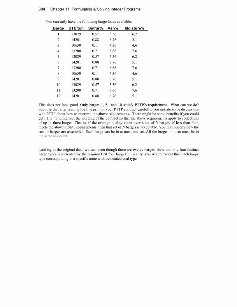
304 Chapter 11 Formulating & Solving Integer Programs
You currently have the following barge loads available.
Barge BTU/ton Sulfur% Ash% Moisture%
1 13029 0.57 5.56 6.2
2 14201 0.88 6.76 5.1
3 10630 0.11 4.36 4.6
4 13200 0.71 6.66 7.6
5 13029 0.57 5.56 6.2
6 14201 0.88 6.76 5.1
7 13200 0.71 6.66 7.6
8 10630 0.11 4.36 4.6
9 14201 0.88 6.76 5.1
10 13029 0.57 5.56 6.2
11 13200 0.71 6.66 7.6
12 14201 0.88 6.76 5.1
This does not look good. Only barges 1, 5, and 10 satisfy PTTP’s requirement. What can we do? Suppose that after reading the fine print of your PTTP contract carefully, you initiate some discussions with PTTP about how to interpret the above requirements. There might be some benefits if you could get PTTP to reinterpret the wording of the contract so that the above requirements apply to collections of up to three barges. That is, if the average quality taken over a set of N barges, N less than four, meets the above quality requirements, then that set of N barges is acceptable. You may specify how the sets of barges are assembled. Each barge can be in at most one set. All the barges in a set must be in the same shipment.
Looking at the original data, we see, even though there are twelve barges, there are only four distinct barge types represented by the original first four barges. In reality, you would expect this: each barge type corresponding to a specific mine with associated coal type.

Formulating & Solving Integer Problems Chapter 11 305
Modeling the barge grouping problem as an assignment problem is relatively straightforward. The essential decision variable is defined as X (I, J) = number of barges of type I assigned to group J. Note we have retained the convention of not distinguishing between barges of the same type. Knowing there are twelve barges, we can restrict ourselves to at most six groups without looking further at the data. The reasoning is: Suppose there are seven nonempty groups. Then, at least two of the groups must be singletons. If two singletons are feasible, then so is the group obtained by combining them. Thus, we can write the following LINGO model:
MODEL:SETS: MINE: BAVAIL; GROUP; QUALITY: QTARG; ! Composition of each type of MINE load; MXQ( MINE, QUALITY): QACT; !assignment of which MINE to which group;!no distinction between types; MXG( MINE, GROUP):X; ENDSETSDATA: MINE = 1..4;
! Barges available of each type(or mine); BAVAIL = 3 4 2 3; QUALITY = BTU, SULF, ASH, MOIST;
! Quality targets as upper limits; QTARG = - 13000 0.63 6.5 7;
! Actual qualities of each mine; QACT = -13029 0.57 5.56 6.2 -14201 0.88 6.76 5.1 -10630 0.11 4.36 4.6 -13200 0.71 6.66 7.6; ! We need at most six groups; GROUP = 1..6; GRPSIZ = 3; ENDDATA! Maximize no. of barges assigned;MAX = @SUM( MXG: X); ! Upper limit on group size;@FOR( GROUP(J): @SUM( MINE( I): X(I, J))
<= GRPSIZ;); ! Assign no more of a type than are available;@FOR( MINE(I): @SUM( GROUP( J): X( I, J)) <= BAVAIL( I)); ! The blending constraints for each group;@FOR( GROUP(J): @FOR( QUALITY ( H): @SUM( MINE( I): X( I, J) * QACT( I, H)) <= @SUM( MINE( I): X( I, J) * QTARG( H));
)); ! barges must be integers;@FOR( MXG: @GIN( X)); END

306 Chapter 11 Formulating & Solving Integer Programs
The following solution shows that you can now sell ten barges, rather than three, to PTTP.
Objective value: 10.00000
Variable ValueX( 1, 1) 1.000000X( 2, 2) 2.000000X( 3, 2) 1.000000X( 1, 4) 2.000000X( 4, 4) 1.000000X( 2, 5) 2.000000X( 3, 5) 1.000000
For example, group 1 is simply one barge of type 1. Group 2 consists two barges of type 2 and one barge of type 3. The above formulation may not scale well. The actual application typically had about 60 barges in a candidate set. The above formulation may be slow to solve problems of that size. The next section discusses how the partitioning approach can be efficiently used for such problems.
Solving with a Partitioning Formulation
Modest-sized integer programs can nevertheless be very difficult to solve. There are a number of rules that are useful when facing such problems. Two useful rules for difficult integer programs are:
1) Do Not Distinguish the Indistinguishable;
2) Presolve subproblems.
The barge matching example can be solved almost “by hand” with the matching or grouping (as opposed to the assignment) approach. Applying the rule “Presolve subproblems,” we can enumerate all feasible combinations of three or less barges selected from the four types. Applying the “Don’t distinguish” rule again, we do not have to consider combinations such as (1,1) and (2,2,2), because such sets are feasible if and only if the singleton sets (e.g., (1) and (2)) are also feasible. Thus, disregarding quality, there are four singleton sets, six doubleton sets, four distinct triplets (e.g., (1,2,3)) and twelve paired triplets (e.g., (1,1,2)) for a total of 26 combinations. It is not hard to show, even manually, that the only feasible combinations are (1), (1,1,4), and (2,2,3). Thus, the matching-like IP we want to solve to maximize the number of barges sold is:
Max = S001 + 3 * S114 + 3 * S223; S001 + 2 * S114 <= 3 ; !(No. of type 1 barges); 2 * S223 <= 4 ; !(No. of type 2 barges); S223 <= 2 ; !(No. of type 3 barges); S114 <= 3 ; !(No. of type 4 barges);
This is easily solved to give S001 = 1, S114 = 1, and S223 = 2, with an objective value of 10.
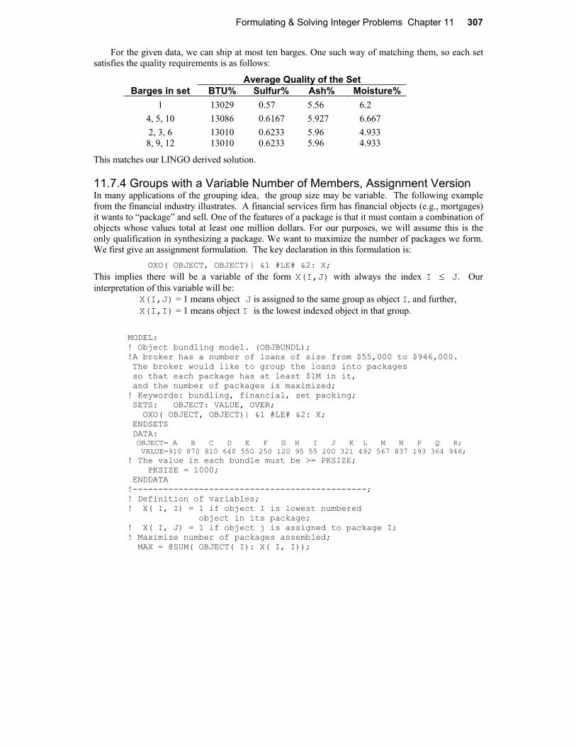
Formulating & Solving Integer Problems Chapter 11 307
For the given data, we can ship at most ten barges. One such way of matching them, so each set satisfies the quality requirements is as follows:
Average Quality of the Set Barges in set BTU% Sulfur% Ash% Moisture%
1 13029 0.57 5.56 6.2
4, 5, 10 13086 0.6167 5.927 6.667
2, 3, 6 13010 0.6233 5.96 4.933 8, 9, 12 13010 0.6233 5.96 4.933
This matches our LINGO derived solution.
11.7.4 Groups with a Variable Number of Members, Assignment Version In many applications of the grouping idea, the group size may be variable. The following example from the financial industry illustrates. A financial services firm has financial objects (e.g., mortgages) it wants to “package” and sell. One of the features of a package is that it must contain a combination of objects whose values total at least one million dollars. For our purposes, we will assume this is the only qualification in synthesizing a package. We want to maximize the number of packages we form. We first give an assignment formulation. The key declaration in this formulation is:
OXO( OBJECT, OBJECT)| &1 #LE# &2: X;
This implies there will be a variable of the form X(I,J) with always the index I J. Our
interpretation of this variable will be:
X(I,J) = 1 means object J is assigned to the same group as object I, and further,
X(I,I) = 1 means object I is the lowest indexed object in that group.
MODEL:! Object bundling model. (OBJBUNDL); !A broker has a number of loans of size from $55,000 to $946,000. The broker would like to group the loans into packages so that each package has at least $1M in it, and the number of packages is maximized; ! Keywords: bundling, financial, set packing; SETS: OBJECT: VALUE, OVER; OXO( OBJECT, OBJECT)| &1 #LE# &2: X; ENDSETS DATA: OBJECT= A B C D E F G H I J K L M N P Q R; VALUE=910 870 810 640 550 250 120 95 55 200 321 492 567 837 193 364 946;
! The value in each bundle must be >= PKSIZE; PKSIZE = 1000; ENDDATA !----------------------------------------------;! Definition of variables; ! X( I, I) = 1 if object I is lowest numbered object in its package; ! X( I, J) = 1 if object j is assigned to package I; ! Maximize number of packages assembled; MAX = @SUM( OBJECT( I): X( I, I));

308 Chapter 11 Formulating & Solving Integer Programs
@FOR( OBJECT( K): ! Each object can be assigned to at most one package; @SUM( OXO( I, K): X( I, K)) <= 1;
! A package must be at least PSIZE in size; @SUM( OXO( K, J): VALUE( J) * X( K, J)) - OVER( K) = PKSIZE * X( K, K); );
! The X( I, J) must = 0 or 1; @FOR( OXO( I, J): @BIN( X( I, J));); END
A solution is:
Variable Value X( A, A) 1.000000 X( A, H) 1.000000 X( B, B) 1.000000 X( B, F) 1.000000 X( C, C) 1.000000 X( C, J) 1.000000 X( D, D) 1.000000 X( D, Q) 1.000000 X( E, E) 1.000000 X( E, L) 1.000000 X( G, G) 1.000000 X( G, K) 1.000000 X( G, M) 1.000000 X( I, I) 1.000000 X( I, R) 1.000000 X( N, N) 1.000000 X( N, P) 1.000000
Thus, eight packages are constructed. Namely: AH, BF, CJ, DQ, EL, IR, JN, GKM, and NP. It happens that every object appears in some package. There are alternate packings of all the objects into eight groups. Thus, one may wish to consider secondary criteria for choosing one alternate optimum over another (e.g., the largest package should be as close as possible to one million in size). The worst package in the fairness sense in the above solution is BF. It is over the target of 1,000,000 by 120,000.
11.7.5 Groups with A Variable Number of Members, Packing Version An alternative approach is first to enumerate either all possible or all interesting feasible groups and then solve an optimization problem of the form:
Maximize value of the groups selected subject to:
Each object is in at most one of the selected groups.
The advantage of this formulation is, when it can be used, it typically can be solved more easily than the assignment formulation. The disadvantages are it may have a huge number of decision variables, especially if the typical group size is more than three. If there are n distinct objects, and all groups are of size k, then there are n!/(k! (n-k)!) distinct groups. For example, if n = 50 and k = 3, then there are 19,600 candidate groups.

Formulating & Solving Integer Problems Chapter 11 309
This formulation uses the idea of composite variables. This is frequently a useful approach for a problem for which the original or “natural” formulation is difficult to solve. Setting a particular composite variable to 1 represents setting a particular combination of the original variables to 1. We generate only those composite variables that correspond to feasible combinations of the original variables. This effectively eliminates many of the fractional solutions that would appear if one solved the LP relaxation of the original formulation. The composite variable idea is a form of what is sometimes called column generation. The path formulation in network models is also an example of the use of composite variables.
Example: Packing Financial Instruments, revisited.
The packing approach to formulating a model for this problem constructs all possible packages or groups that just satisfy the one million minimum. The general form of the LP/IP is:
Maximize value of packages selected subject to:
Each object appears in at most one selected package.
In the formulation below, we will use sparse sets to represent our packages. We assume that we need not consider packages of more than four objects. An attractive feature of the packing/partitioning formulation is that we can easily attach an essentially arbitrary score to each possible group. In particular, the following formulation applies a squared penalty to the extent to which a package of loans exceeds the target of $1M.
MODEL:! Object bundling model. (OBJBUNDH);! A broker has a number of loans of size from $55,000 to $946,000. The broker would like to group the loans into packages so that each package has at least $1M in it, preferably not much more, and the number of packages is maximized;! Keywords: bundling, financial, set packing;SETS: OBJECT: VALUE; ENDSETSDATA:
OBJECT = A B C D E F G H I J K L M N P Q R; VALUE = 910 870 810 640 550 250 120 95 55 200 321 492 567 837 193 364 946;
! The value in each bundle must be >= PKSIZE; PKSIZE = 1000; ENDDATASETS:
!Enumerate all 2,3, and 4 object unordered sets package size; BNDL2( OBJECT, OBJECT) | &1 #LT# &2 #AND# (VALUE(&1) + VALUE(&2)) #GE# PKSIZE: X2, OVER2; BNDL3( OBJECT, OBJECT, OBJECT) | &1 #LT# &2 #AND# &2 #LT# &3

310 Chapter 11 Formulating & Solving Integer Programs
#AND# ( VALUE(&1) + VALUE(&2) + VALUE(&3) #GE# PKSIZE): X3, OVER3; BNDL4( OBJECT, OBJECT, OBJECT, OBJECT) | &1 #LT# &2 #AND# &2 #LT# &3 #AND# &3 #LT# &4 #AND# (( VALUE(&1) + VALUE(&2) + VALUE(&3) + VALUE( &4)) #GE# PKSIZE): X4, OVER4;ENDSETS!----------------------------------------------;!Compute the overage of each bundle;@FOR( BNDL2( I,J):
OVER2(I,J) = VALUE(I) + VALUE(J) - PKSIZE; ); @FOR( BNDL3( I,J,K):
OVER3(I,J,K) = VALUE(I)+VALUE(J)+VALUE(K) - PKSIZE ); @FOR( BNDL4( I,J,K,L):
OVER4(I,J,K,L) = VALUE(I)+VALUE(J)+VALUE(K)+VALUE(L)- PKSIZE; );
! Maximize score of packages assembled. Penalize a package that is over the minimum package size;MAX= @SUM( BNDL2( I,J): X2(I,J) * (1-(OVER2(I,J)/PKSIZE)^2))
+@SUM( BNDL3( I,J,K): X3(I, J,K) * (1-(OVER3(I,J,K)/PKSIZE)^2)) + @SUM( BNDL4( I,J,K,L): X4(I,J,K,L) * (1-(OVER4(I,J,K,L)/PKSIZE)^2));
@FOR( OBJECT( M): ! Each object M can be in at most one of the selected bundles;
@SUM( BNDL2( I, J)| I #EQ# M #OR# J #EQ# M: X2( I, J)) + @SUM( BNDL3( I, J, K)| I #EQ# M #OR# J #EQ# M #OR# K #EQ# M: X3( I, J, K)) + @SUM( BNDL4( I, J, K, L)| I #EQ# M #OR# J #EQ# M #OR# K #EQ# M #OR# L #EQ# M: X4( I, J, K, L)) <= 1; );
! The X's must = 0 or 1;@FOR( BNDL2( I, J): @BIN( X2( I, J));); @FOR( BNDL3( I, J, K): @BIN( X3( I, J, K));); @FOR( BNDL4( I, J, K, L): @BIN( X4( I, J, K, L)););
END

Formulating & Solving Integer Problems Chapter 11 311
Global optimal solution found at iteration: 19 Objective value: 7.989192 Variable Value X2( A, H) 1.000000 OVER2( A, H) 5.000000 X2( B, P) 1.000000 OVER2( B, P) 63.00000 X2( C, F) 1.000000 OVER2( C, F) 60.00000 X2( D, Q) 1.000000 OVER2( D, Q) 4.000000 X2( E, L) 1.000000 OVER2( E, L) 42.00000 X2( I, R) 1.000000 OVER2( I, R) 1.000000 X2( J, N) 1.000000 OVER2( J, N) 37.00000 X3( G, K, M) 1.000000 OVER3( G, K, M) 8.000000
Notice that this allocation is slightly more balanced than the previous solution based on the assignment formulation. The largest “overage” is 63,000 rather than 120,000. This is because the grouping formulation provided an easy way to penalize large packages.
11.7.6 Groups with A Variable Number of Members, Cutting Stock Problem
Another application in which the partitioning or packing approach has worked well is the cutting stock problem in the paper and steel industry. We revisit the example introduced in chapter 7. There we manually enumerated all possible patterns or packings drawn from 8 different finished good widths into each of three different raw material widths. The formulation below automatically enumerates all possible patterns. For each raw material width, the formulation automatically enumerates all possible groupings of 1, 2, …,7 finished good widths so that the sum of the finished good widths is less than or equal to the raw material width. One notable feature of this formulation is that it introduces a shortcut that may be important in keeping computation time low when there are many, e.g., more than 20, objects. To illustrate the shortcut, consider the three declarations:
! Enumerate all possible cutting patterns with 1 fg; rxf(rm,fg)| lenf(&2) #le# lenr(&1): x1; ! Enumerate all possible patterns with 2 fg; rxf2( rxf, fg) | &2 #le# &3 #and# (lenf(&2) + lenf(&3) #le# lenr(&1)): x2; ! Enumerate all possible patterns with 3 fg; rxf3( rxf2, fg)| &3 #le# &4 #and# (lenf(&2) + lenf(&3)+ lenf(&4) #le# lenr(&1)): x3;

312 Chapter 11 Formulating & Solving Integer Programs
The declaration rxf(rm,fg), by itself, tells LINGO to generate all combinations of one raw
material and one finished good. The condition | lenf(&2) #le# lenr(&1) , however, tells
LINGO to not generate a combination of a raw material(the index &1) and finished good(index &2) for which the length(or width depending upon your orientation) of the finished good is greater than
that of the raw material. So, for example, the combination (R36, F38) will not be a member of
rxf. There will be four elements in rxf for which the first item of the pair is R36, namely ( R36,
F34), (R36, F24), ( R36, F15), and ( R36, F10).
Now consider how to generate all feasible combinations containing two finished good widths.
The obvious declaration would be: rxf2( rm, fg, fg) | &2 #le# &3 #and# (lenf(&2) + lenf(&3) #le# lenr(&1))
The condition &2 #le# &3 says we do not care about the order of the finished goods in the
pattern, so we might as well restrict ourselves to listing the finished goods in the pattern in sorted
order. The condition lenf(&2) + lenf(&3) #le# lenr(&1) restricts the elements of set
rxf2 to feasible ones. This declaration would be valid, but we did not do it. Why? Instead we used
the declaration rxf2( rxf, fg). The latter was used mainly for computational reasons. With the
latter, LINGO considers every combination of the elements of the set rxf and each finished good.
Consider the case when the raw material is r36. If the declaration rxf2( rm, fg, fg) is used,
then LINGO would look at 8 * 8 = 64 combinations of two finished goods and keep only the four
combinations (r36, f24, f10 ), (r36, f15, f15 ), (r36, f15, f10 ), and (r36, f10,
f10 ). If on the other hand, the declaration rxf2( rxf, fg) is used, then when the raw material
is R36, LINGO will only consider 4*8 = 32 combinations. The 4 arises because set rxf contains
only 4 elements for which the first member of the pair is R36. For sets rxf3, and higher, the
computational savings can be even higher.
! Cutting stock solver(cutgent);! Keywords: cutting stock;sets:! Each raw material has a size(length) and quantity; rm: lenr, qr; ! Ditto for each finished good; fg: lenf, qf; endsetsdata:! Describe the raw materials available; rm, lenr, qr = R72 72 9999 R45 48 9999 R36 36 9999; ! Describe the finished goods needed; fg, lenf, qf = F60 60 500 F56 56 400 F42 42 300 F38 38 450 F34 34 350 F24 24 100

Formulating & Solving Integer Problems Chapter 11 313
F15 15 800 F10 10 1000; enddata
sets:! Enumerate all possible cutting patterns with 1 fg; rxf(rm,fg)| lenf(&2) #le# lenr(&1): x1; ! Enumerate all possible patterns with 2 fg; rxf2( rxf, fg) | &2 #le# &3 #and# (lenf(&2) + lenf(&3) #le# lenr(&1)): x2;! Enumerate all possible patterns with 3 fg; rxf3( rxf2, fg)| &3 #le# &4 #and# (lenf(&2) + lenf(&3)+ lenf(&4) #le# lenr(&1)): x3;! Enumerate all possible patterns with 4 fg; rxf4( rxf3, fg)| &4 #le# &5 #and# (lenf(&2) + lenf(&3) + lenf(&4)+lenf(&5) #le# lenr(&1)): x4;! Enumerate all possible patterns with 5 fg; rxf5( rxf4, fg)| &5 #le# &6 #and# (lenf(&2) + lenf(&3)+ lenf(&4)+lenf(&5)+lenf(&6) #le# lenr(&1)): x5; ! Enumerate all possible patterns with 6 fg; rxf6( rxf5, fg)| &6 #le# &7 #and# (lenf(&2) + lenf(&3)+ lenf(&4)+lenf(&5) +lenf(&6)+lenf(&7) #le# lenr(&1)): x6;
endsets! Minimize length of material used;
min = @sum( rxf(r,f1): lenr(r)*x1(r,f1)) + @sum( rxf2(r,f1,f2): lenr(r)*x2(r,f1,f2)) + @sum( rxf3(r,f1,f2,f3): lenr(r)*x3(r,f1,f2,f3)) + @sum( rxf4(r,f1,f2,f3,f4): lenr(r)*x4(r,f1,f2,f3,f4)) + @sum( rxf5(r,f1,f2,f3,f4,f5): lenr(r)*x5(r,f1,f2,f3,f4,f5)) + @sum( rxf6(r,f1,f2,f3,f4,f5,f6): lenr(r)*x6(r,f1,f2,f3,f4,f5,f6));
! We have to satisfy each finished good demand;@for( fg(f):
@sum(rxf(r,f): x1(r,f)) + @sum(rxf2(r,f1,f2)| f #eq# f1: x2(r,f1,f2)) + @sum(rxf2(r,f1,f2)| f #eq# f2: x2(r,f1,f2)) + @sum(rxf3(r,f1,f2,f3)| f #eq# f1: x3(r,f1,f2,f3)) + @sum(rxf3(r,f1,f2,f3)| f #eq# f2: x3(r,f1,f2,f3)) + @sum(rxf3(r,f1,f2,f3)| f #eq# f3: x3(r,f1,f2,f3))

314 Chapter 11 Formulating & Solving Integer Programs
+ @sum(rxf4(r,f1,f2,f3,f4)| f #eq# f1: x4(r,f1,f2,f3,f4)) + @sum(rxf4(r,f1,f2,f3,f4)| f #eq# f2: x4(r,f1,f2,f3,f4)) + @sum(rxf4(r,f1,f2,f3,f4)| f #eq# f3: x4(r,f1,f2,f3,f4)) + @sum(rxf4(r,f1,f2,f3,f4)| f #eq# f4: x4(r,f1,f2,f3,f4)) + @sum(rxf5(r,f1,f2,f3,f4,f5)| f #eq# f1: x5(r,f1,f2,f3,f4,f5)) + @sum(rxf5(r,f1,f2,f3,f4,f5)| f #eq# f2: x5(r,f1,f2,f3,f4,f5)) + @sum(rxf5(r,f1,f2,f3,f4,f5)| f #eq# f3: x5(r,f1,f2,f3,f4,f5)) + @sum(rxf5(r,f1,f2,f3,f4,f5)| f #eq# f4: x5(r,f1,f2,f3,f4,f5)) + @sum(rxf5(r,f1,f2,f3,f4,f5)| f #eq# f5: x5(r,f1,f2,f3,f4,f5)) + @sum(rxf6(r,f1,f2,f3,f4,f5,f6)| f #eq# f1: x6(r,f1,f2,f3,f4,f5,f6)) + @sum(rxf6(r,f1,f2,f3,f4,f5,f6)| f #eq# f2: x6(r,f1,f2,f3,f4,f5,f6)) + @sum(rxf6(r,f1,f2,f3,f4,f5,f6)| f #eq# f3: x6(r,f1,f2,f3,f4,f5,f6)) + @sum(rxf6(r,f1,f2,f3,f4,f5,f6)| f #eq# f4: x6(r,f1,f2,f3,f4,f5,f6)) + @sum(rxf6(r,f1,f2,f3,f4,f5,f6)| f #eq# f5: x6(r,f1,f2,f3,f4,f5,f6)) + @sum(rxf6(r,f1,f2,f3,f4,f5,f6)| f #eq# f6: x6(r,f1,f2,f3,f4,f5,f6)) >= qf(f); );
! We cannot use more raw material than is available;@for( rm( r):
@sum(rxf(r,f): x1(r,f)) + @sum(rxf2(r,f1,f2): x2(r,f1,f2)) + @sum(rxf3(r,f1,f2,f3): x3(r,f1,f2,f3)) + @sum(rxf4(r,f1,f2,f3,f4): x4(r,f1,f2,f3,f4)) + @sum(rxf5(r,f1,f2,f3,f4,f5): x5(r,f1,f2,f3,f4,f5)) + @sum(rxf6(r,f1,f2,f3,f4,f5,f6): x6(r,f1,f2,f3,f4,f5,f6)) <= qr(r); );
! Can only run integer quantities of each pattern;@for(rxf: @gin(x1));@for(rxf2: @gin(x2));@for(rxf3: @gin(x3));@for(rxf4: @gin(x4));@for(rxf5: @gin(x5));@for(rxf6: @gin(x6));

Formulating & Solving Integer Problems Chapter 11 315
If you click on LINGO | Generate menu item, to display the scaler version of the model, you can see that the constraint for the 56 inch width is(hopefully reassuringly):
X2_R72_F56_F15 + X2_R72_F56_F10 + X1_R72_F56 >= 400 ;
When we click on the Solve icon we get the solution:
Global optimal solution found at iteration: 31 Objective value: 119832.0
Variable Value X2( R72, F60, F10) 500.0000 X2( R72, F56, F15) 400.0000 X2( R72, F38, F34) 350.0000 X3( R72, F42, F15, F15) 186.0000 X3( R72, F38, F24, F10) 100.0000 X4( R72, F42, F10, F10, F10) 114.0000 X4( R45, F15, F10, F10, F10) 2.000000 X6( R72, F15, F15, F10, F10, F10, F10) 13.00000
11.7.7 Groups with A Variable Number of Members, Vehicle Routing The following vehicle routing example demonstrates that you can in fact perform a little optimization computation as part of the column or group generation. The example we use is a variation of the vehicle routing problem considered in section 11.6.3. The first and major part of this model is devoted to enumerating all minimal feasible trips with at most seven stops. By feasible trip, we mean that the amount of material to be delivered to the stops in the trip does not exceed the vehicle capacity of 18 pallets. By minimal we mean that for a trip that visits a given set of stops, the trip visits the stops in a sequence that minimizes the distance traveled. Given that all minimal feasible trips have been generated, the following simple integer program is solved: Minimize Cost of trips selected; Subject to: For each stop: Exactly one trip includes this stop.
This little example has 15 stops, so the integer program has 15 constraints, and a large number of 0/1 variables(about 7300 in fact) , equal in number to the number of minimal feasible trips.
The tricky part is how we generate the sets of minimal feasible trips, PSET2, PSET3, etc. and the assocated minimal distances, D2( ), D3( ), etc. To start understanding ideas, consider the variable
D4(I,J,K,L). It has the following definition.
D4(I,J,K,L) = minimum distance required to start at the depot, visit stops I, J, and K in
any order and then visit stop L. If DIST(I,J) is the distance matrix, then Held and Karp(1962)
observed that if D3 is defined in similar fashion, then D4 can be computed by the dynamic
programming recursion: D4(I,J,K,L) = min[D3(I,J,K)+DIST(K,L), D3(I,K,J)+DIST(J,L), D3(J,K,I)+DIST(I,L)]
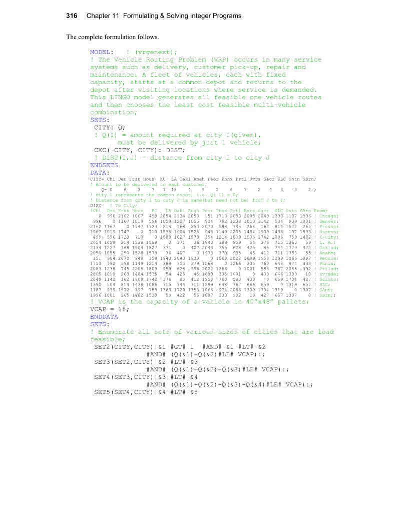
316 Chapter 11 Formulating & Solving Integer Programs
The complete formulation follows.
MODEL: ! (vrgenext);! The Vehicle Routing Problem (VRP) occurs in many servicesystems such as delivery, customer pick-up, repair andmaintenance. A fleet of vehicles, each with fixedcapacity, starts at a common depot and returns to thedepot after visiting locations where service is demanded. This LINGO model generates all feasible one vehicle routes and then chooses the least cost feasible multi-vehicle combination;SETS: CITY: Q; ! Q(I) = amount required at city I(given), must be delivered by just 1 vehicle; CXC( CITY, CITY): DIST; ! DIST(I,J) = distance from city I to city JENDSETSDATA:CITY= Chi Den Frsn Hous KC LA Oakl Anah Peor Phnx Prtl Rvrs Sacr SLC Sntn SBrn; ! Amount to be delivered to each customer; Q= 0 6 3 7 7 18 4 5 2 6 7 2 4 3 3 2 ; ! city 1 represents the common depot, i.e. Q( 1) = 0;! Distance from city I to city J is same(but need not be) from J to I;DIST= ! To City;!Chi Den Frsn Hous KC LA Oakl Anah Peor Phnx Prtl Rvrs Sacr SLC Sntn SBrn From; 0 996 2162 1067 499 2054 2134 2050 151 1713 2083 2005 2049 1390 1187 1996 ! Chcago; 996 0 1167 1019 596 1059 1227 1055 904 792 1238 1010 1142 504 939 1001 ! Denver;2162 1167 0 1747 1723 214 168 250 2070 598 745 268 162 814 1572 265 ! Fresno;1067 1019 1747 0 710 1538 1904 1528 948 1149 2205 1484 1909 1438 197 1533 ! Huston; 499 596 1723 710 0 1589 1827 1579 354 1214 1809 1535 1742 1086 759 1482 ! K-City;2054 1059 214 1538 1589 0 371 36 1943 389 959 54 376 715 1363 59 ! L. A.;2134 1227 168 1904 1827 371 0 407 2043 755 628 425 85 744 1729 422 ! Oaklnd;2050 1055 250 1528 1579 36 407 0 1933 379 995 45 412 711 1353 55 ! Anahm; 151 904 2070 948 354 1943 2043 1933 0 1568 2022 1889 1958 1299 1066 1887 ! Peoria;1713 792 598 1149 1214 389 755 379 1568 0 1266 335 760 648 974 333 ! Phnix;2083 1238 745 2205 1809 959 628 995 2022 1266 0 1001 583 767 2086 992 ! Prtlnd;2005 1010 268 1484 1535 54 425 45 1889 335 1001 0 430 666 1309 10 ! Rvrsde;2049 1142 162 1909 1742 376 85 412 1958 760 583 430 0 659 1734 427 ! Scrmto;1390 504 814 1438 1086 715 744 711 1299 648 767 666 659 0 1319 657 ! SLC;1187 939 1572 197 759 1363 1729 1353 1066 974 2086 1309 1734 1319 0 1307 ! SAnt;1996 1001 265 1482 1533 59 422 55 1887 333 992 10 427 657 1307 0 ! SBrn;;
! VCAP is the capacity of a vehicle in 40”x48” pallets;VCAP = 18; ENDDATASETS:! Enumerate all sets of various sizes of cities that are load feasible; SET2(CITY,CITY)|&1 #GT# 1 #AND# &1 #LT# &2 #AND# (Q(&1)+Q(&2)#LE# VCAP):; SET3(SET2,CITY)|&2 #LT# &3 #AND# (Q(&1)+Q(&2)+Q(&3)#LE# VCAP):; SET4(SET3,CITY)|&3 #LT# &4 #AND# (Q(&1)+Q(&2)+Q(&3)+Q(&4)#LE# VCAP):; SET5(SET4,CITY)|&4 #LT# &5

Formulating & Solving Integer Problems Chapter 11 317
#AND# (Q(&1)+Q(&2)+Q(&3)+Q(&4)+Q(&5)#LE# VCAP):; SET6(SET5,CITY)|&5 #LT# &6 #AND# (Q(&1)+Q(&2)+Q(&3)+Q(&4)+Q(&5)+Q(&6)#LE# VCAP):; SET7(SET6,CITY)|&6 #LT# &7 #AND# (Q(&1)+Q(&2)+Q(&3)+Q(&4)+Q(&5)+Q(&6)+Q(&7)#LE# VCAP):;
! Enumerate all partially ordered sets with a specific city as the last one; PSET2(CITY,CITY)| &1 #GT# 1 #AND# &1#NE#&2 #AND# (Q(&1)+Q(&2)#LE# VCAP): D2,X2; PSET3(SET2,CITY)| &1#NE#&3 #AND# &2#NE#&3 #AND# (Q(&1)+Q(&2)+Q(&3)#LE# VCAP): D3,X3; PSET4(SET3,CITY)| &1#NE#&4 #AND# &2#NE#&4 #AND# &3 #NE# &4 #AND# (Q(&1)+Q(&2)+Q(&3)+Q(&4)#LE# VCAP): D4,X4; PSET5(SET4,CITY)| &1#NE#&5 #AND# &2#NE#&5 #AND# &3 #NE# &5 #AND# &4 #NE# &5 #AND# (Q(&1)+Q(&2)+Q(&3)+Q(&4)+Q(&5)#LE# VCAP): D5,X5; PSET6(SET5,CITY)| &1#NE#&6 #AND# &2#NE#&6 #AND# &3 #NE# &6 #AND# &4 #NE# &6 #AND# &5 #NE# &6 #AND# (Q(&1)+Q(&2)+Q(&3)+Q(&4)+Q(&5)+Q(&6)#LE# VCAP): D6,X6; PSET7(SET6,CITY)| &1#NE#&7 #AND# &2#NE#&7 #AND# &3#NE#&7 #AND# &4#NE#&7 #AND# &5#NE#&7 #AND# &6#NE#&7 #AND# (Q(&1)+Q(&2)+Q(&3)+Q(&4)+Q(&5)+Q(&6)+Q(&7)#LE# VCAP): D7,X7;ENDSETS
! Compute shortest distance to visit all cities in PSET, and ending up at last city in each partially ordered set, using Held&Karp DP. Essential idea: DS( S,t) = minimum distance to visit all cities in S and then end up at t. The recursion is: DS( S, t) = min{k in S: DS(S-k,k) + DIST(k,t)};@FOR(PSET2(I,J): D2(I,J) = DIST(1,I) + DIST(I,J); @BIN(X2);
); @FOR(PSET3(I,J,K):! @SMIN is the min of a list of scalers. D3(I,J,K) = min cost of

318 Chapter 11 Formulating & Solving Integer Programs
starting at 1, visiting I and J in some order, and then K; D3(I,J,K) = @SMIN( D2(I,J) + DIST(J,K), D2(J,I) + DIST(I,K));@BIN(X3);
); @FOR(PSET4(I,J,K,L):!D4(I,J,K,L) = min cost of starting at 1, visiting I, J, & K in some order, and then L; D4(I,J,K,L) =
@SMIN( D3(I,J,K)+DIST(K,L), D3(I,K,J)+DIST(J,L), D3(J,K,I)+DIST(I,L));
@BIN( X4); );
@FOR(PSET5(I,J,K,L,M): D5(I,J,K,L,M) =
@SMIN( D4(I,J,K,L)+DIST(L,M), D4(I,J,L,K)+DIST(K,M), D4(I,K,L,J)+DIST(J,M), D4(J,K,L,I)+DIST(I,M));
@BIN(X5); );
@FOR(PSET6(I,J,K,L,M,N): D6(I,J,K,L,M,N) =
@SMIN( D5(I,J,K,L,M)+DIST(M,N), D5(I,J,K,M,L)+DIST(L,N), D5(I,J,L,M,K)+DIST(K,N), D5(I,K,L,M,J)+DIST(J,N), D5(J,K,L,M,I)+DIST(I,N)); @BIN(X6);
);
@FOR(PSET7(I,J,K,L,M,N,P): D7(I,J,K,L,M,N,P) =
@SMIN( D6(I,J,K,L,M,N)+DIST(N,P), D6(I,J,K,L,N,M)+DIST(M,P), D6(I,J,K,M,N,L)+DIST(L,P), D6(I,J,L,M,N,K)+DIST(K,P), D6(I,K,L,M,N,J)+DIST(J,P), D6(J,K,L,M,N,I)+DIST(I,P)); @BIN(X7);
);
! and finally, the optimization model... Min cost of routes chosen, over complete routes ending back at 1;

Formulating & Solving Integer Problems Chapter 11 319
Min = + @SUM( PSET2(I,J)| J #EQ# 1: D2(I,J)*X2(I,J)) + @SUM( PSET3(I,J,K)| K #EQ# 1: D3(I,J,K)*X3(I,J,K)) + @SUM( PSET4(I,J,K,L)| L #EQ# 1: D4(I,J,K,L)*X4(I,J,K,L)) + @SUM( PSET5(I,J,K,L,M)| M #EQ# 1: D5(I,J,K,L,M)*X5(I,J,K,L,M)) + @SUM( PSET6(I,J,K,L,M,N)| N #EQ# 1:
D6(I,J,K,L,M,N)*X6(I,J,K,L,M,N)) + @SUM( PSET7(I,J,K,L,M,N,P)| P #EQ# 1:
D7(I,J,K,L,M,N,P)*X7(I,J,K,L,M,N,P));
! Each city must be on exactly one complete route;@FOR( CITY(I1)| I1 #GT# 1: + @SUM( PSET2(I,J) | J #EQ# 1 #AND# ( I #EQ# I1): X2(I,J)) + @SUM( PSET3(I,J,K) |K #EQ# 1 #AND# (I#EQ#I1 #OR# J#EQ# I1): X3(I,J,K)) + @SUM( PSET4(I,J,K,L) |L #EQ# 1 #AND# (I#EQ#I1 #OR# J#EQ# I1 #OR# K#EQ# I1): X4(I,J,K,L)) + @SUM( PSET5(I,J,K,L,M) |M #EQ# 1 #AND# (I#EQ#I1 #OR# J#EQ# I1 #OR# K#EQ# I1 #OR# L#EQ#I1): X5(I,J,K,L,M)) + @SUM( PSET6(I,J,K,L,M,N) |N #EQ# 1 #AND# (I#EQ#I1 #OR# J#EQ# I1 #OR# K#EQ# I1 #OR# L#EQ#I1 #OR# M#EQ#I1): X6(I,J,K,L,M,N)) + @SUM( PSET7(I,J,K,L,M,N,P) |P #EQ# 1 #AND# (I#EQ#I1 #OR# J#EQ#I1 #OR# K#EQ#I1 #OR# L#EQ#I1 #OR# M#EQ#I1 #OR# N#EQ#I1) : X7(I,J,K,L,M,N,P)) = 1;
);
It takes about 4 seconds to get the following solution
Global optimal solution found at iteration: 134 Objective value: 17586.00
Variable Value X2( LA, CHI) 1.000000 X3( KC, PEOR, CHI) 1.000000 X4( DEN, HOUS, SNTN, CHI) 1.000000 X5( FRSN, OAKL, PRTL, SACR, CHI) 1.000000 X6( ANAH, PHNX, RVRS, SLC, SBRN, CHI) 1.000000
The obvious question is, how well does this formulation scale up? The final set partitioning integer program is not too challenging. The big challenge is generating and storing the possibly huge number

320 Chapter 11 Formulating & Solving Integer Programs
of trips. A crucial consideration is the number of stops per trip. If this is small, e.g., three, then the number of trips will be manageable. A typical vehicle routing problem may have around 100 stops. The number of possible minimal distance trips, each of which visit three out of 100 stops, is 100!/[3!97!] = 161,700. This is a manageable number of variables for an efficient IP solver.
11.8 Linearizing Products of Variables We have previously seen products of 0/1 variables, such as y1 y2 and y1
2 can be represented by linear expressions by means of a simple transformation. This transformation generalizes to the case of the product of a 0/1 variable and a continuous variable.
To illustrate, suppose the product x y appears in a model, where y is 0/1 while x is nonnegative continuous. We want to replace this nonlinear component by a (somewhat bigger) linear component. If
we have an upper bound (Mx) on the value of x, an upper bound (My) on the product x y, and we
define P = x y, then the following linear constraints will cause P to take on the correct value:
P x
P My y
P x Mx (1 y)
Hanson and Martin (1990) show how this approach is useful in setting prices for products when we allow bundling of products. Bundle pricing is a form of quantity discounting. Examples of products that might be bundled are (a) airfare, hotel, rental car, tours, and meals or (b) computer, monitor, printer, and hard disk. Stigler (1963) showed how a movie distributor might improve profits by leasing bundles of movies rather than leasing individual movies. Bundling assumes it is easy for the seller to assemble the bundle and difficult for a buyer to unbundle. Otherwise, a reseller could buy the bundle at a discount and then sell the individual components at a markup.
11.8.1 Example: Bundling of Products Microland Software has recently acquired an excellent word processing product to complement its own recently developed spreadsheet product. Microland is contemplating offering the combination of the two products for a discount. After demonstrating the products at a number of diverse professional meetings, Microland developed the following characterization of the market:
Maximum Price Market Segment is Willing To Pay for Various Bundles
MarketSegment
Size in 10,000
Spreadsheet Only
Wordprocessor Only Both
Business/Scientific
7 450 110 530
Legal/Administrative
5 75 430 480
Educational 6 290 250 410
Home 4.5 220 380 390
We will refer to each market segment as simply a “customer”. Economic theory suggests a customer will buy the product that gives the greatest consumer surplus, where consumer surplus is defined as the price the customer is willing to pay for the product (the “reservation price”) minus the market price for the product. For example, if the prices for the three bundles, spreadsheet only, word

Formulating & Solving Integer Problems Chapter 11 321
processor only, and both together, were set respectively at 400, 150, and 500, then the
business/scientific market would buy the spreadsheet alone because the consumer surplus is 50 vs. 40 and 30 for the other two bundles. To give a general model of this situation, define:
Rij = reservation price of customer i for bundle j,Ni = “size of customer” i (i.e., number of individual customers in segment i), si = consumer surplus achieved by customer i,yij = 1 if customer i buys bundle j, 0 otherwise, xj = price of bundle j set by the seller.
We will treat the empty bundle as just another bundle, so we can say every customer buys exactly one bundle. The seller, Microland, would like to choose the xj to:
Maximize ji
Ni yij xj
The fact that each customer will buy exactly one bundle is enforced with:
For each customer i:
jyij = 1
For each customer i, its achieved consumer surplus is:
si = j
(Rij xj)yij
Customer i will buy only the bundle j for which its consumer surplus, si, is the maximum. This is enforced by the constraints:
For each customer i and bundle j:
si Rij xj
A difficulty with the objective function and the consumer surplus constraints is they involve the product yijxj. Let us follow our previous little example and replace the product yijxj by Pij. If Mj is an upper bound on xj, then, proceeding as before, to enforce the definition Pij = yijxj, we need the constraints:
Pij xj
Pij Rij yij
Pij xj (1 yij)Mj.

322 Chapter 11 Formulating & Solving Integer Programs
Making these adjustments to the model, we get:
Maximize ji
Ni Pij
subject to: For each customer i
jyij = 1;
For each customer i, bundle j:
si Rij xj;For each customer i:
si = j
(Rij yij Pij);
To enforce the nonlinear condition Pij = yij xj, we have for each i and j:
Pij xj
Pij Rij yij
Pij xj (1 yij)Mj.
For all i and j:
yij = 0 or 1
In explicit form, the LINGO model is:
MODEL:SETS:MARKET/B, L, E, H/:S, N; ITEM/NONE, SO, WO, BOTH/:X; CROSS(MARKET, ITEM):R, Y, P;
ENDSETSDATA:N = 7, 5, 6, 4.5; R = 0 450 110 530 0 75 430 480 0 290 250 410 0 220 380 390;
ENDDATA

Formulating & Solving Integer Problems Chapter 11 323
MAX = @SUM(CROSS(I, J): P(I, J) * N(I)); !Make the PICK variables 0/1; @FOR(CROSS:@BIN(PICK));!Each customer buys exactly one bundle; @FOR(MARKET(I): @SUM(ITEM(J): Y(I, J)) = 1); !Each customer's achieved surplus, SURP, must be at least as good from every possible bundle; @FOR(ITEM(I): @FOR(MARKET(J): X(I) + S(J) >= R(J, I))); !Compute the achieved surplus; @FOR(MARKET(I): @SUM(ITEM(J): P(I, J) - R(I, J) * Y(I, J)) + S(I) = 0); ! Each product variable Pij must be.. ; ! <= Xj ; ! <= Rij * Yij ; ! >= Xj M + M * Yij ; M = 600; !Max price of any bundle; @FOR(CROSS(I, J): P(I, J) <= X(J); P(I, J) <= Y(I, J) * R(I, J); R(I, J) >= X(J) - M + M * Y(I, J);); ! Price of bundle should be < sum of component prices; X(BOTH) <= X(SO) + X(WO); ! Price of bundle should be > any one component; X(BOTH) >= X(SO); X(BOTH) >= X(WO);
END
For the Microland problem, the solution is to set the following prices:
Spreadsheet Only Word Processing Only Both
Bundle Price: 410 380 410
Thus, the business, legal and educational markets will buy the bundle of both products. The home market will buy only the word processor. Total revenues obtained by Microland are 90,900,000. The interested reader may show that, if bundling is not possible, then the highest revenue that Microland can achieve is only 67,150,000.
11.9 Representing Logical Conditions For some applications, it may be convenient, perhaps even logical, to state requirements using logical expressions. A logical variable can take on only the values TRUE or FALSE. Likewise, a logical expression involving logical variables can take on only the values TRUE or FALSE. There are two major logical operators, .AND. and .OR., that are useful in logical expressions. The logical expression:
A .AND. B
is TRUE if and only if both A and B are true. The logical expression:
A .OR. B
is TRUE if and only if at least one of A and B is true.

324 Chapter 11 Formulating & Solving Integer Programs
It is sometimes useful also to have the logical operator implication ( ) written as follows:
A B
with the meaning that if A is true, then B must be true. Logical variables are trivially representable by binary variables with:
TRUE being represented by 1, and FALSE being represented by 0.
If A, B, and C are 0/1 variables, then the following constraint combinations can be used to represent the various fundamental logical expressions:
Logical Expression Mathematical Constraints
C = A .AND. B C A
C B
C A + B 1
C = A .OR. B C A
C B
C A + B
A C A C
11.10 Problems 1. The following problem is known as a segregated storage problem. A feed processor has various
amounts of four different commodities, which must be stored in seven different silos. Each silo can contain at most one commodity. Associated with each commodity and silo combination is a loading cost. Each silo has a finite capacity, so some commodities may have to be split over several silos. For a similar problem arising in the loading of fuel tank trucks at Mobil Oil Company, see Brown, Ellis, Graves, and Ronen (1987). The following table contains the data for this problem.
Loading Cost per Ton
SiloAmount of Commodity
Commodity 1 2 3 4 5 6 7To Be Stored
A $1 $2 $2 $3 $4 $5 $5 75 tons
B 2 3 3 3 1 5 5 50 tons
C 4 4 3 2 1 5 5 25 tons
D 1 1 2 2 3 5 5 80 tons
Silo Capacity in Tons 25 25 40 60 80 100 100

Formulating & Solving Integer Problems Chapter 11 325
a) Present a formulation for solving this class of problems.
b) Find the minimum cost solution for this particular example.
c) How would your formulation change if additionally there was a fixed cost associated with each silo that is incurred if anything is stored in the silo?
2. You are the scheduling coordinator for a small, growing airline. You must schedule exactly one flight out of Chicago to each of the following cities: Atlanta, Los Angeles, New York, and Peoria. The available departure slots are 8 A.M., 10 A.M., and 12 noon. Your airline has only two departure lounges, so at most two flights can be scheduled per slot. Demand data suggest the following expected profit contribution per flight as a function of departure time:
Expected Profit Contribution in $1000’s Time
Destination 8 10 12
Atlanta 10 9 8.5
Los Angeles 11 10.5 9.5
New York 17 16 15
Peoria 6.4 2.5 1
Formulate a model for solving this problem.
3. A problem faced by an electrical utility each day is that of deciding which generators to start up at which hour based on the forecast demand for electricity each hour. This problem is also known as the unit commitment problem. The utility in question has three generators with the following characteristics:
Generator
FixedStartup
Cost
Fixed Cost per Period
of Operation
Cost per Period per Megawatt
Used
Maximum Capacity in Megawatts Each
Period
A 3000 700 5 2100
B 2000 800 4 1800
C 1000 900 7 3000
There are two periods in a day and the number of megawatts needed in the first period is 2900. The second period requires 3900 megawatts. A generator started in the first period may be used in the second period without incurring an additional startup cost. All major generators (e.g., A, B, and C above) are turned off at the end of each day.
a) First, assume fixed costs are zero and thus can be disregarded. What are the decision variables?
b) Give the LP formulation for the case where fixed costs are zero.
c) Now, take into account the fixed costs. What are the additional (zero/one) variables to define?
d) What additional terms should be added to the objective function? What additional constraints should be added?

326 Chapter 11 Formulating & Solving Integer Programs
4. Crude Integer Programming. Recently, the U.S. Government began to sell crude oil from its Naval Petroleum Reserve in sealed bid auctions. There are typically six commodities or products to be sold in the auction, corresponding to the crude oil at the six major production and shipping points. A “bid package” from a potential buyer consists of (a) a number indicating an upper limit on how many barrels (bbl.) the buyer is willing to buy overall in this auction and (b) any number of “product bids”. Each product bid consists of a product name and three numbers representing, respectively, the bid price per barrel of this product, the minimum acceptable quantity of this product at this price, and the maximum acceptable quantity of this product at this price. Not all product bids of a buyer need be successful. The government usually places an arbitrary upper limit (e.g., 20%) on the percentage of the total number of barrels over all six products one firm is allowed to purchase.
To illustrate the principal ideas, let us simplify slightly and suppose there are only two supply sources/products, which are denoted by A and B. There are 17,000 bbls. available at A while B has 13,000. Also, there are only two bidders, the Mobon and the Exxil companies. The government arbitrarily decides either one can purchase at most 65% of the total available crude. The two bid packages are as follows:
Mobon: Maximum desired = 16,000 bbls. total.
ProductBid per Barrel
MinimumBarrels
Accepted
MaximumBarrels Wanted
A 43 9000 16,000
B 51 6000 12,000
Exxil: Maximum desired = No limit.
ProductBid per Barrel
MinimumBarrels
Accepted
MaximumBarrels Wanted
A 47 5000 10,000
B 50 5000 10,000
Formulate and solve an appropriate IP for the seller.

Formulating & Solving Integer Problems Chapter 11 327
5. A certain state allows a restricted form of branch banking. Specifically, a bank can do business in county i if the bank has a “principal place of business” in county i or in a county sharing a nonzero-length border with county i. Figure 11.9 is a map of the state in question:
Figure 11.9 Districts in a State
Formulate the problem of locating a minimum number of principal places of business in the state, so a bank can do business in every county in the state. If the problem is formulated as a covering problem, how many rows and columns will it have? What is an optimal solution? Which formulation is tighter: set covering or simple plant location?
6. Data Set Allocation Problem. There are 10 datasets or files, each of which is to be allocated to 1 of 3 identical disk storage devices. A disk storage device has 885 cylinders of capacity. Within a storage device, a dataset will be assigned to a contiguous set of cylinders. Dataset sizes and interactions between datasets are shown in the table below. Two datasets with high interaction rates should not be assigned to the same device. For example, if datasets C and E are assigned to the same disk, then an interaction cost of 46 is incurred. If they are assigned to different disks, there is no interaction cost between C and E.

328 Chapter 11 Formulating & Solving Integer Programs
Dataset for Interaction (Seek Transition) Rates
A B C D E F G H I J
Dataset Size in
Cylinders
A 110
B 43 238
C 120 10 425
D 57 111 188 338
E 96 78 46 88 55
F 83 58 421 60 63 391
G 77 198 207 109 73 74 267
H 31 50 43 47 51 21 88 105
I 38 69 55 21 36 391 47 96 256
J 212 91 84 53 71 40 37 35 221 64
2249
Find an assignment of datasets to disks, so total interaction cost is minimized and no disk capacity is exceeded.
7. The game or puzzle of mastermind pits two players, a “coder” and a “decoder”, against each other. The game is played with a pegboard and a large number of colored pegs. The pegboard has an
array of 4 12 holes. For our purposes, we assume there are only six colors: red, blue, clear, purple, gold, and green. Each peg has only one color. The coder starts the game by selecting four pegs and arranging them in a fixed order, all out of sight of the decoder. This ordering remains fixed throughout the game and is appropriately called the code. At each play of the game, the decoder tries to match the coder’s ordering by placing four pegs in a row on the board. The coder then provides two pieces of information about how close the decoder’s latest guess is to the coder’s order:
1) The number of pegs in the correct position (i.e., color matching the coder’s peg in that position), and
2) The maximum number of pegs that would be in correct position if the decoder were allowed to permute the ordering of the decoder’s latest guess.
Call these two numbers m and n. The object of the decoder is to discover the code in a minimum number of plays.

Formulating & Solving Integer Problems Chapter 11 329
The decoder may find the following IP of interest.
MAX = XRED1; XRED1 + XBLUE1 + XCLEAR1 + XPURP1 + XGOLD1 + XGREEN1 = 1; XRED2 + XBLUE2 + XCLEAR2 + XPURP2 + XGOLD2 + XGREEN2 = 1; XRED3 + XBLUE3 + XCLEAR3 + XPURP3 + XGOLD3 + XGREEN3 = 1; XRED4 + XBLUE4 + XCLEAR4 + XPURP4 + XGOLD4 + XGREEN4 = 1; XRED1 + XRED2 + XRED3 + XRED4 - RED = 0; XBLUE1 + XBLUE2 + XBLUE3 + XBLUE4 - BLUE = 0; XCLEAR1 + XCLEAR2 + XCLEAR3 + XCLEAR4 - CLEAR = 0; XPURP1 + XPURP2 + XPURP3 + XPURP4 - PURP = 0; XGOLD1 + XGOLD2 + XGOLD3 + XGOLD4 - GOLD = 0; XGREEN1 + XGREEN2 + XGREEN3 + XGREEN4 - GREEN = 0; END
All variables are required to be integer. The interpretation of the variables is as follows. XRED1 = 1 if a red peg is in position 1, otherwise 0, etc.; XGREEN4 = 1 if a green peg is in position 4, otherwise 0. Rows 2 through 5 enforce the requirement that exactly one peg be placed in each position. Rows 6 through 11 are simply accounting constraints, which count the number of pegs of each color. For example, RED = the number of red pegs in any position 1 through 4. The objective is unimportant. All variables are (implicitly) required to be nonnegative.
At each play of the game, the decoder can add new constraints to this IP to record the information gained. Any feasible solution to the current formulation is a reasonable guess for the next play. An interesting question is what constraints can be added at each play.
To illustrate, suppose the decoder guesses the solution XBLUE1 = XBLUE2 = XBLUE3 = XRED4 = 1, and the coder responds with the information that
m = 1 and m n = 1. That is, one peg is in the correct position and, if permutations were allowed, at most two pegs would be in the correct position. What constraints can be added to the IP to incorporate the new information?
8. The Mathematical Football League (MFL) is composed of M teams (M is even). In a season of
2(M 1) consecutive Sundays, each team will play (2M 1) games. Each team must play each other team twice, once at home and once at the other team’s home stadium. Each Sunday, k games from the MFL are televised. We are given a matrix {vij} where vij is the viewing audience on a given Sunday if a game between teams i and j playing at team j’s stadium is televised.
a) Formulate a model for generating a schedule for the MFL that maximizes the viewing audience over the entire season. Assume viewing audiences are additive.
b) Are some values of k easier to accommodate than others? How?

330 Chapter 11 Formulating & Solving Integer Programs
9. The typical automobile has close to two dozen electric motors. However, if you examine these motors, you will see that only about a half dozen distinct motor types are used. For inventory and maintenance reasons, the automobile manufacturer would like to use as few distinct types as possible. For cost, quality, and weight reasons, one would like to use as many distinct motor types as possible, so the most appropriate motor can be applied to each application. The table below describes the design possibilities for a certain automobile:
24-Month Failure Probability Number
Required Motor type
Application A B C D E
Head lamps 2 0.002 0.01 0.01 0.007
Radiator fan 2 0.01 0.002 0.004
Wipers 2 0.007
Seat 4 0.003 0.006 0.008
Mirrors 2 0.004 0.001
Heater fan 1 0.006 0.001
Sun roof 1 0.002 0.003 0.009
Windows 4 0.004 0.008 0.005
Antenna 1 0.003 0.003 0.002
Weight 2 3 1.5 1 4
Cost per Motor
24 20 36 28 39
For example, two motors are required to operate the headlamps. If type D motors are used for headlamps, then the estimated probability of a headlamp motor failure in two years is about 0.01. If no entry appears for a particular combination of motor type and application, it means the motor type is inappropriate for that application (e.g., because of size).
Formulate a solvable linear integer program for deciding which motor type to use for each application, so at most 3 motor types are used, the total weight of the motors used is at most 36, total cost of motors used is at most 585, and probability of any failure in two years is approximately minimized.
10. We have a rectangular three-dimensional container that is 30 50 50. We want to pack in it
rectangular three-dimensional boxes of the three different sizes: (a) 5 5 10, (b) 5 10 10,
and (c) 5 15 25.
A particular packing of boxes into the container is undominated if there is no other packing that contains at least as many of each of the three box types and strictly more of one of the box types.
Show there are no more than 3101 undominated packings.

Formulating & Solving Integer Problems Chapter 11 331
11. Given the following:
Checkerboard and domino
If two opposite corners of the checkerboard are made unavailable, prove there is no way of exactly covering the remaining grid with 31 dominoes.
12. Which of the following requirements could be represented exactly with linear constraints? (You are allowed to use transformations if you wish.)
(a) (3 x + 4 y)/(2 x + 3 y) 12; (b) MAX (x, y) < 8;
(c) 3 x + 4 y y 11; where y is 0 or 1;
(d) ABS (10 x) 7 (Note ABS means absolute value); (e) MIN (x, y) < 12.
13. A common way of controlling access in many systems, such as information systems or the military, is with priority levels. Each user i is assigned a clearance level Ui. Each object j is assigned a security level Lj. A user i does not have access to object j if the security level of j is higher than the clearance level of i. Given a set of users; and, for each user, a list of objects to which that user does not to have access; and a list of objects to which the user should have access, can we assign Ui’s and Lj’s, so these access rights and denials are satisfied? Formulate as an integer program.
14. One of the big consumption items in the U.S. is automotive fuel. Any petroleum distributor who can deliver this fuel reliably and efficiently to the hundreds of filling stations in a typical distribution region has a competitive advantage. This distribution problem is complicated by the fact that a typical customer (i.e., filling station) requires three major products: premium gasoline, an intermediate octane grade (e.g., “Silver”), and regular gasoline. A typical situation is described below. A delivery tank truck has four compartments with capacities in liters of 13,600, 11,200, 10,800, and 4400. We would like to load the truck according to the following limits:
Liters of Premium Intermediate Regular
At least: 8,800 12,000 12,800
At most: 13,200 17,200 16,400
Only one gasoline type can be stored per compartment in the delivery vehicle. Subject to the previous considerations, we would like to maximize the amount of fuel loaded on the truck.
(a) Define the decision variables you would use in formulating this problem as an IP. (b) Give a formulation of this problem. (c) What allocation do you recommend?

332 Chapter 11 Formulating & Solving Integer Programs
15. Most lotteries are of the form:
Choose n numbers (e.g., n = 6) from the set of numbers {1, 2, ..., m} (e.g., m = 54).
You win the grand prize if you buy a ticket and choose a set of n numbers identical to the nnumbers eventually chosen by lottery management. Smaller prizes are awarded to people who match k of the n numbers. For n = 6, typical values for k are 4 and 5. Consider a modest little lottery with m = 7, n = 3, and k = 2. How many tickets would you have to buy to guarantee winning a prize? Can you set this up as a grouping/covering problem?
16. A recent marketing phenomenon is the apparent oxymoron, “mass customization”. The basic idea is to allow each customer to design his/her own product, and yet do it on an efficient, high-volume scale. A crucial component of the process is to automate the final design step involving the customer. As an example, IBM and Blockbuster recently announced a plan to offer “on-demand” production of customized music products at retail stores. Each store would carry an electronic “master” for every music piece a customer might want. The physical copy for the customer would then be produced for the customer while they wait. This opens up all manners of opportunities for highly customized musical products. Each customer might provide a list of songs to be placed on an audiocassette. A design issue when placing songs on a two-sided medium such as a cassette is how to allocate songs to sides. A reasonable rule is to distribute the songs, so the playing times on the two sides are as close to equal as possible. For an automatic tape player, this will minimize the “dead time” when switching from one side to another. As an example, we mention that Willie Nelson has recorded the following ten songs in duets with other performers:
Song Time (min:secs) Other Performer
1) Pancho and Lefty 4:45 Merle Haggard
2) Slow Movin Outlaw 3:35 Lacy J. Dalton
3) Are There any More Real Cowboys
3:03 Neil Young
4) I Told a Lie to My Heart 2:52 Hank Williams
5) Texas on a Saturday Night 2:42 Mel Tillis
6) Seven Spanish Angels 3:50 Ray Charles
7) To All the Girls I’ve Loved Before
3:30 Julio Iglesias
8) They All Went to Mexico 4:45 Carlos Santana
9) Honky Tonk Women 3:30 Leon Russell
10) Half a Man 3:02 George Jones
You want to collect these songs on a two-sided tape cassette album to be called “Half Nelson.”
(a) Formulate and solve an integer program for minimizing the dead time on the shorter side.
(b) What are some of the marketing issues of allowing the customer to decide which song goes on which side?

Formulating & Solving Integer Problems Chapter 11 333
17. Bill Bolt is hosting a party for his daughter Lydia on the occasion of her becoming of college age. He has reserved a banquet room with 18 tables at the Racquet Club on Saturday night. Each table can accommodate at most 8 people. A total of 140 young people are coming, 76 young men and 64 young ladies. Lydia and her mother, Jane, would like to have the sexes as evenly distributed as possible at the tables. They want to have at least 4 men and at least 3 women at each table.
(a) Is it possible to have an allocation satisfying the above as well as the restriction there be at most 4 men at each table?
(b) Provide a good allocation of the sexes to the tables.
18. The game or puzzle of Clue is played with a deck of 21 cards. At the beginning of a game, three of the cards are randomly selected and placed face down in the center of the table. The remaining cards are distributed face down as evenly as possible to the players. Each player may look at his or her own cards. The object of the game is to correctly guess the three cards in the center. At each player’s turn, the player is allowed to either guess the identity of the three cards in the center or ask any other player a question of the form: “Do you have any of the following three cards?” (The asking player then publicly lists the three cards.) If the asked player has one of the three identified cards, then the asked player must show one of the cards to the asking player (and only to the asking player). Otherwise, the asked player simply responds “No”. If a player correctly guesses the three cards in the center, then that player wins. If a player incorrectly guesses the three cards in the center, the player is out of the game.
Deductions about the identity of various cards can be made if we define:
X (i, j) = 1 if player i has card j, else 0.
Arbitrarily define the three cards in the center as player 1. Thus, we can initially start with the constraints:
X jj
( , )11
21
= 3.
For each card, j = 1, 2, …, 21:
X i ji
( , ) = 1.
(a) Suppose player 3 is asked: “Do you have either card 4, 8, or 17?” and player 3 responds “No.” What constraint can be added?
(b) Suppose in response to your question in (a), player 3 shows you card 17. What constraint can be added?
(c) What LP would you solve in order to determine whether card 4 must be one of the cards in the center?
Note, in the “implementation” of the game marketed in North America, the 21 cards are actually divided into three types: (i) six suspect cards with names like “Miss Scarlet,” (ii) six weapons cards with names like “Revolver,” and (c) nine room cards with names like “Kitchen.” This has essentially no effect on our analysis above.