Copyright © Cengage Learning. All rights reserved.

10.9 Systems Of Inequalities

2

Objectives

► Graphing an Inequality

► Systems of Inequalities

► Systems of Linear Inequalities

► Application: Feasible Regions

3

Graphing an Inequality

4

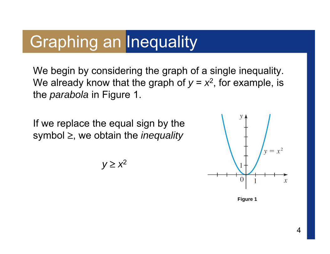
Graphing an InequalityWe begin by considering the graph of a single inequality. We already know that the graph of y = x2, for example, is the parabola in Figure 1.

If we replace the equal sign by the symbol , we obtain the inequality

y x2

Figure 1

5

Graphing an InequalityIts graph consists of not just the parabola in Figure 1, but also every point whose y-coordinate is larger than x2.

We indicate the solution in Figure 2(a) by shading the points above the parabola.

(a) y x2

Figure 2

6

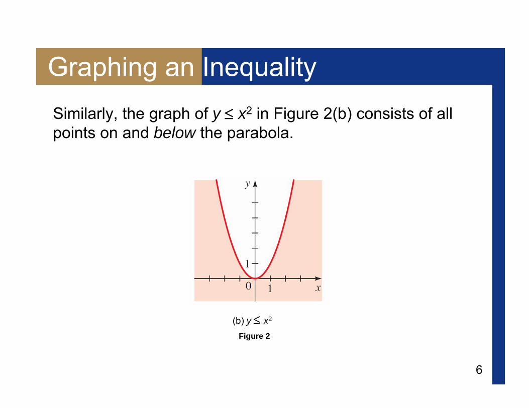
Graphing an InequalitySimilarly, the graph of y x2 in Figure 2(b) consists of all points on and below the parabola.

(b) y x2

Figure 2

7

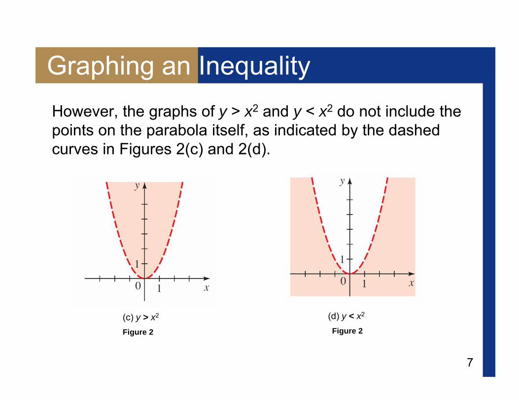
Graphing an InequalityHowever, the graphs of y > x2 and y < x2 do not include the points on the parabola itself, as indicated by the dashed curves in Figures 2(c) and 2(d).

(d) y < x2

Figure 2(c) y > x2

Figure 2

8

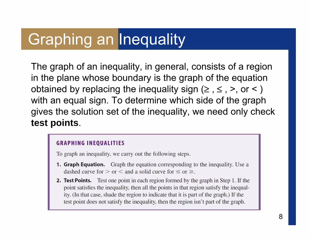
Graphing an InequalityThe graph of an inequality, in general, consists of a region in the plane whose boundary is the graph of the equation obtained by replacing the inequality sign ( , , >, or < ) with an equal sign. To determine which side of the graph gives the solution set of the inequality, we need only check test points.

9

Example 1 – Graphs of InequalitiesGraph each inequality.

(a) x2 + y2 < 25 (b) x + 2y 5

Solution:(a) The graph of x2 + y2 = 25 is a circle of radius 5 centered

at the origin.

10

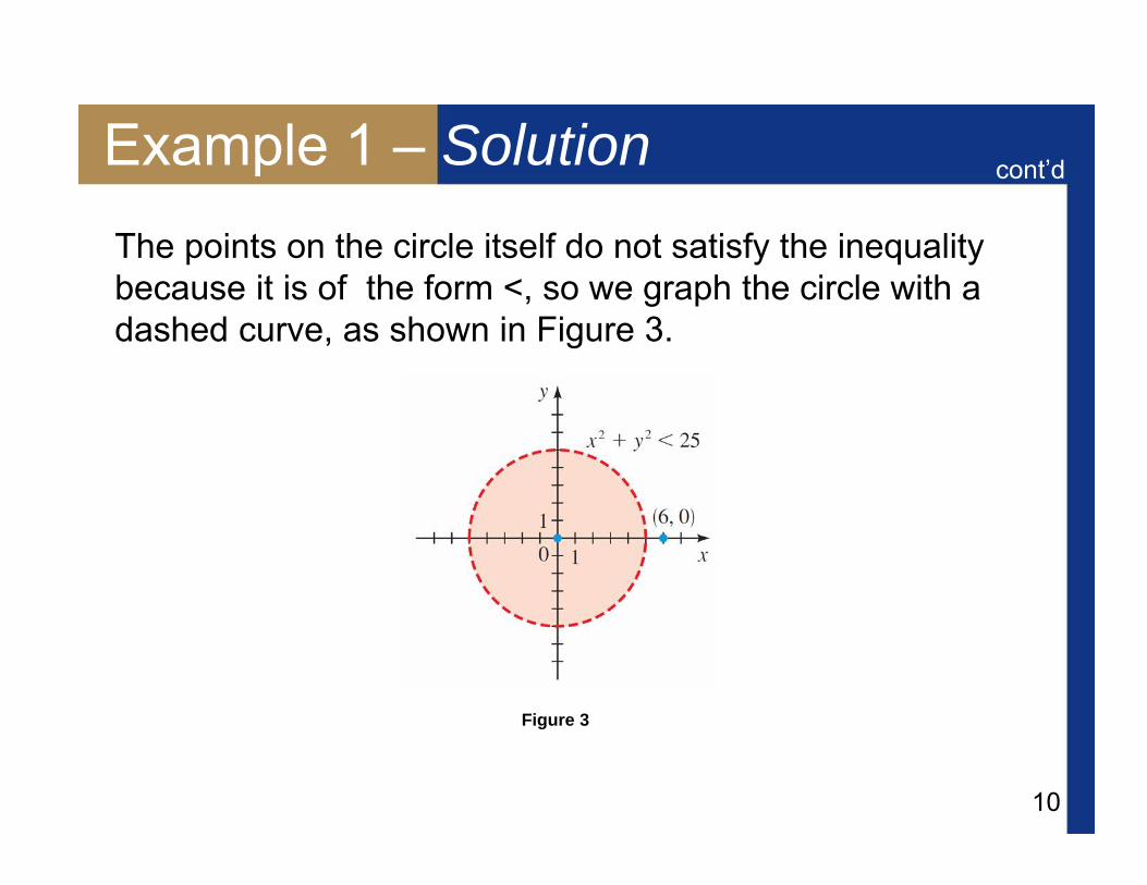
Example 1 – SolutionThe points on the circle itself do not satisfy the inequality because it is of the form <, so we graph the circle with a dashed curve, as shown in Figure 3.

Figure 3

cont’d

11

Example 1 – SolutionTo determine whether the inside or the outside of the circle satisfies the inequality, we use the test points (0,0) on the inside and (6, 0) on the outside.

To do this, we substitute the coordinates of each point into the inequality and check whether the result satisfies the inequality.

cont’d

12

Example 1 – SolutionNote that any point inside or outside the circle can serve as a test point. We have chosen these points for simplicity.

Thus the graph of x2 + y2 < 25 is the set of all points inside the circle (see Figure 3).

cont’d

Figure 3

13

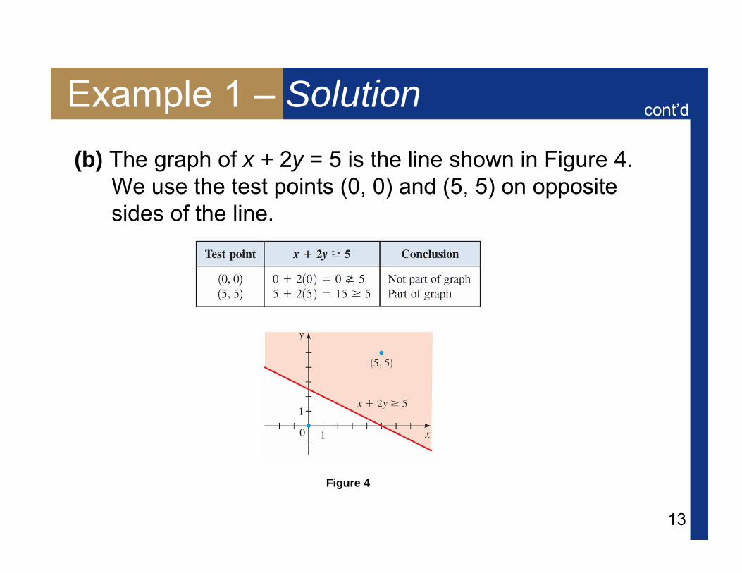
Example 1 – Solution(b) The graph of x + 2y = 5 is the line shown in Figure 4.

We use the test points (0, 0) and (5, 5) on opposite sides of the line.

Figure 4

cont’d

14

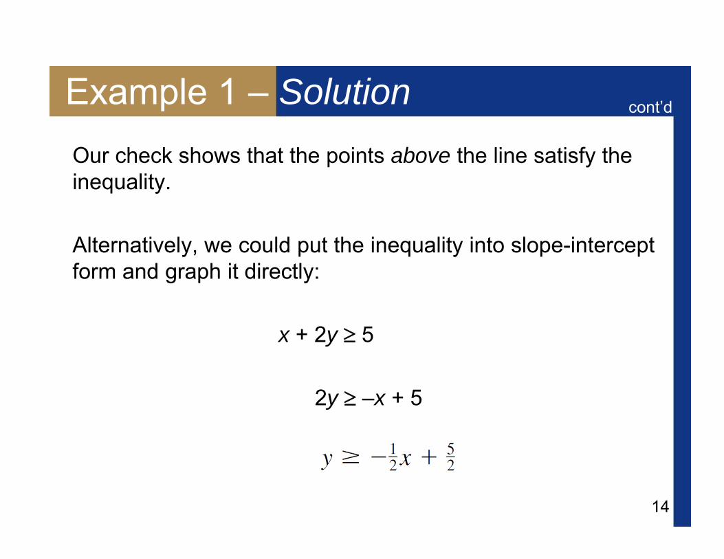
Example 1 – SolutionOur check shows that the points above the line satisfy the inequality.

Alternatively, we could put the inequality into slope-intercept form and graph it directly:

x + 2y 5

2y –x + 5

cont’d

15

Example 1 – SolutionFrom this form we see that the graph includes all points whose y-coordinates are greater than those on the line

; that is, the graph consists of the points on or above this line, as shown in Figure 4.

cont’d

Figure 4

16

Systems of Inequalities

17

Systems of InequalitiesWe now consider systems of inequalities.

The solution of such a system is the set of all points in the coordinate plane that satisfy every inequality in the system.

18

Example 2 – A System of Two Inequalities

Graph the solution of the system of inequalities, and label its vertices.

x2 + y2 < 25x + 2y 5

Solution:These are the two inequalities of Example 1. In this example we wish to graph only those points that simultaneously satisfy both inequalities.

The solution consists of the intersection of the graphs in Example 1.

19

Example 2 – SolutionIn Figure 5(a) we show the two regions on the same coordinate plane (in different colors), and in Figure 5(b) we show their intersection.

(a) (b)x2 + y2 < 25x + 2y 5

cont’d

Figure 5

20

Example 2 – SolutionVertices The points (–3, 4) and (5, 0) in Figure 5(b) are the vertices of the solution set. They are obtained by solving the system of equations

x2 + y2 = 25x + 2y = 5

We solve this system of equations by substitution.

cont’d

21

Example 2 – SolutionSolving for x in the second equation gives x = 5 – 2y, and substituting this into the first equation gives

(5 – 2y)2 + y2 = 25

(25 – 20y + 4y2) + y2 = 25

–20y + 5y2 = 0

–5y(4 – y) = 0

Thus y = 0 or y = 4.

Substitute x = 5 – 2y

Expand

Factor

Simplify

cont’d

22

Example 2 – SolutionWhen y = 0, we have x = 5 – 2(0) = 5, and when y = 4, we have x = 5 – 2(4) = –3. So the points of intersection of these curves are (5, 0) and (–3, 4).

Note that in this case the vertices are not part of the solution set, since they don’t satisfy the inequality x2 + y2 < 25 (so they are graphed as open circles in the figure). They simply show where the “corners” of the solution set lie.

cont’d

23

Systems of Linear Inequalities

24

Systems of Linear InequalitiesAn inequality is linear if it can be put into one of the following forms:

ax + by c ax + by c ax + by > c ax + by < c

In the next example we graph the solution set of a system of linear inequalities.

25

Example 3 – A System of Four Linear Inequalities

Graph the solution set of the system, and label its vertices.

x + 3y 12x + y 8

x 0 y 0

26

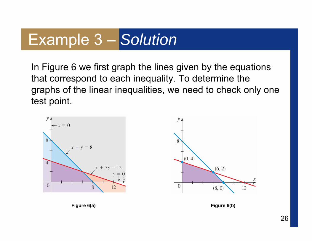
Example 3 – SolutionIn Figure 6 we first graph the lines given by the equations that correspond to each inequality. To determine the graphs of the linear inequalities, we need to check only one test point.

Figure 6(b)Figure 6(a)

27

Example 3 – SolutionFor simplicity let’s use the point (0, 0).

Since (0, 0) is below the line x + 3y = 12, our check shows that the region on or below the line must satisfy the inequality.

cont’d

28

Example 3 – SolutionLikewise, since (0, 0) is below the line x + y = 8, our check shows that the region on or below this line must satisfy the inequality.

The inequalities x 0 and y 0 say that x and y are nonnegative.

cont’d

29

Example 3 – SolutionThese regions are sketched in Figure 6(a), and the intersection—the solution set—is sketched in Figure 6(b).

Figure 6(b)Figure 6(a)

cont’d

30

Example 3 – SolutionVertices The coordinates of each vertex are obtained by simultaneously solving the equations of the lines that intersect at that vertex. From the system

x + 3y = 12x + y = 8

we get the vertex (6, 2). The origin (0, 0) is also clearly a vertex. The other two vertices are at the x- and y-intercepts of the corresponding lines: (8, 0) and (0, 4). In this case all the vertices are part of the solution set.

cont’d

31

Systems of Linear InequalitiesWhen a region in the plane can be covered by a (sufficiently large) circle, it is said to be bounded. A region that is not bounded is called unbounded.

32

Systems of Linear InequalitiesFor example, the region graphed in Figure 8 is bounded, whereas the region in Figure 4 is unbounded. An unbounded region cannot be “fenced in”—it extends infinitely far in at least one direction.

Figure 8 Figure 4

33

Application: Feasible Regions

34

Application: Feasible RegionsMany applied problems involve constraints on the variables. For instance, a factory manager has only a certain number of workers who can be assigned to perform jobs on the factory floor.

A farmer deciding what crops to cultivate has only a certain amount of land that can be seeded. Such constraints or limitations can usually be expressed as systems of inequalities.

When dealing with applied inequalities, we usually refer to the solution set of a system as a feasible region, because the points in the solution set represent feasible (or possible) values for the quantities being studied.

35

Example 5 – Restricting Pollutant Outputs

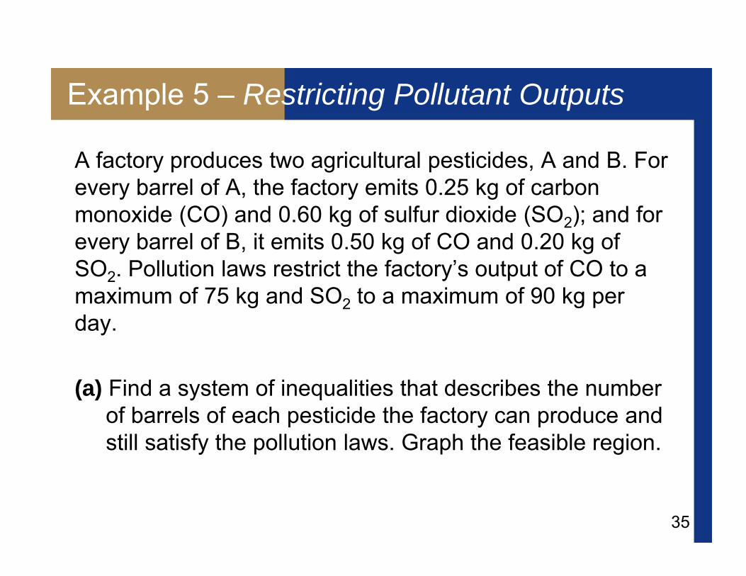
A factory produces two agricultural pesticides, A and B. For every barrel of A, the factory emits 0.25 kg of carbon monoxide (CO) and 0.60 kg of sulfur dioxide (SO2); and for every barrel of B, it emits 0.50 kg of CO and 0.20 kg of SO2. Pollution laws restrict the factory’s output of CO to a maximum of 75 kg and SO2 to a maximum of 90 kg per day.

(a) Find a system of inequalities that describes the number of barrels of each pesticide the factory can produce and still satisfy the pollution laws. Graph the feasible region.

36

Example 5 – Restricting Pollutant Outputs

(b) Would it be legal for the factory to produce 100 barrels of A and 80 barrels of B per day?

(c) Would it be legal for the factory to produce 60 barrels of A and 160 barrels of B per day?

Solution:(a) To set up the required inequalities, it is helpful to

organize the given information into a table.

cont’d

37

Example 5 – SolutionWe let

x = number of barrels of A produced per day

y = number of barrels of B produced per day

From the data in the table and the fact that x and y can’t be negative, we obtain the following inequalities.

0.25x + 0.50y 750.60x + 0.20y 90x 0, y 0

CO inequality

SO2 inequality

cont’d

38

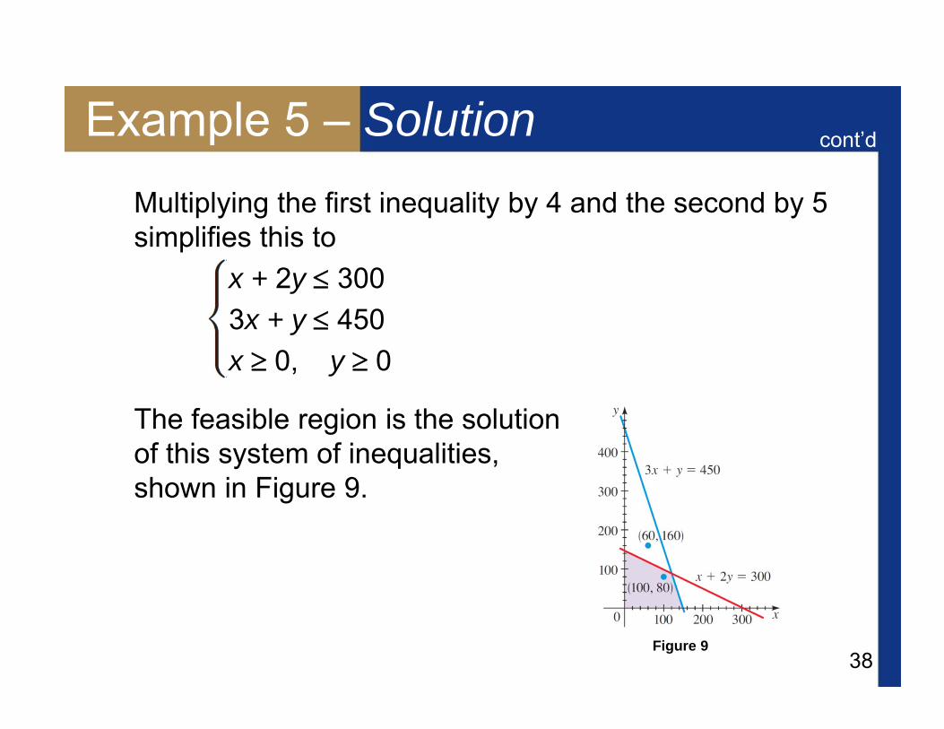
Example 5 – SolutionMultiplying the first inequality by 4 and the second by 5 simplifies this to

x + 2y 3003x + y 450x 0, y 0

The feasible region is the solution of this system of inequalities, shown in Figure 9.

Figure 9

cont’d

39

Example 5 – Solution(b) Since the point (100, 80) lies inside the feasible region,

this production plan is legal (see Figure 9).

(c) Since the point (60, 160) lies outside the feasible region, this production plan is not legal. It violates the CO restriction, although it does not violate the SO2restriction (see Figure 9).

cont’d