106-2 cp08 多維度資料格式homepage.ntu.edu.tw/~fengli/Teaching/Computer/106-2_cp08.pdf ·...

連豊力臺大電機系

Feb 2018 - Jun 2018

106-2: EE4052

計算機程式設計

Computer Programming

通識課程：

之旅

通識課程：

之旅

計算機程式設計 – 2018S

U08: 多維度資料

Feng-Li Lian @ NTU-EE

2

課程主題進度

U01: 課程介紹：討論主題，作業，報告，進行方式

U02: 主題，案例，程式，演算法，資源

U03: 設定軟體 R 與 Rstudio

U04: 數據處理與繪圖指令功能

U05: 資料類別與基本運算

U06: 邏輯判斷與流程控制

U07: 函數：計算與排序

U08: 多維度資料格式

U09: 檔案資料輸入與輸出

U10: 繪圖功能與文字

U11: 多重繪圖與顏色

U12: 函數：動畫與動作

U13: 探索性資料分析

U14: 資料間的相關性

U15: 資料連結分析

•資料格式




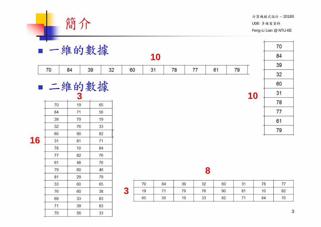
一維的數據

二維的數據

簡介

10

10

16

3

3

8

3




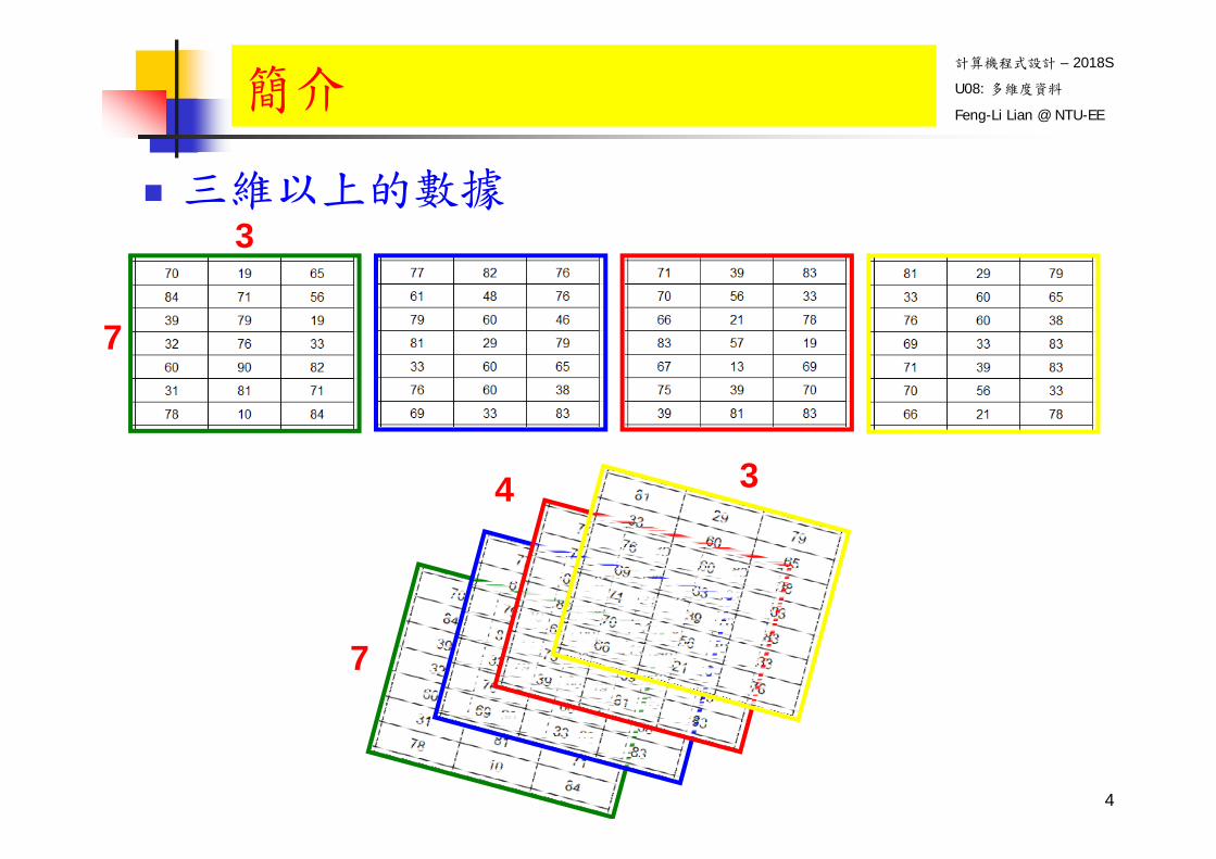
三維以上的數據

簡介

3

7

3

7

4

4




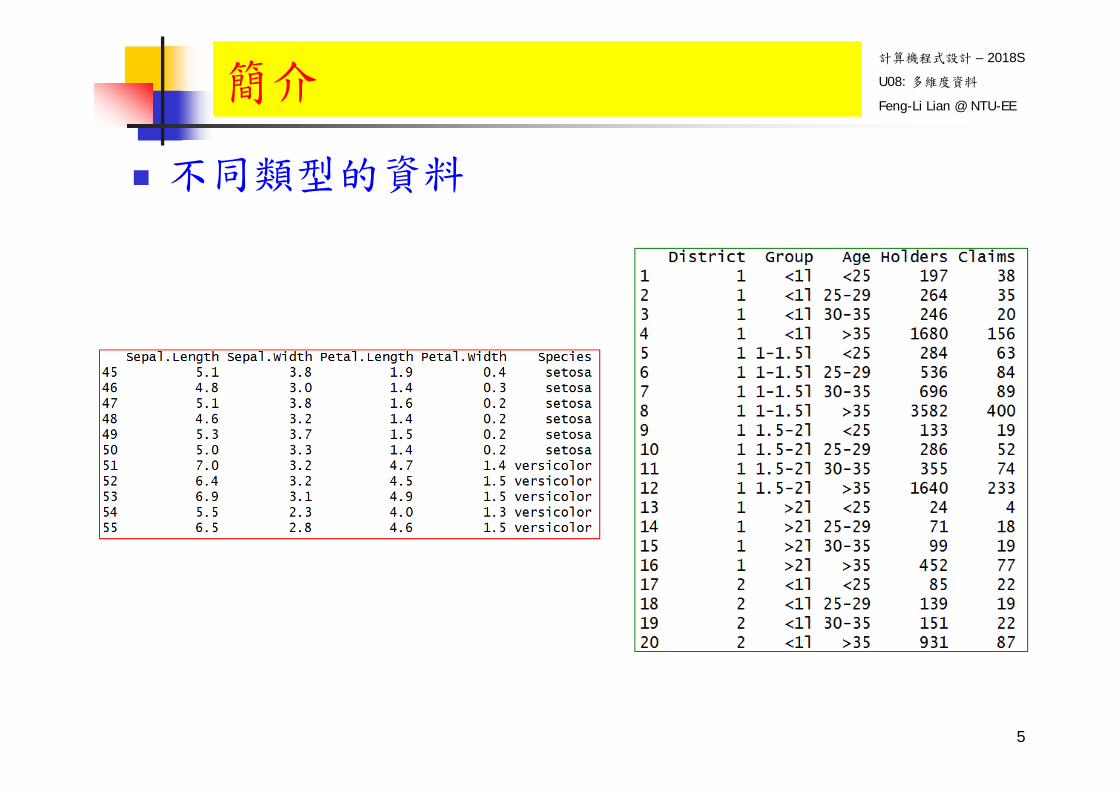
不同類型的資料

簡介

5



Feng-Li Lian @ NTU-EE大綱

作業

6



Feng-Li Lian @ NTU-EEHW06：多維度資料格式

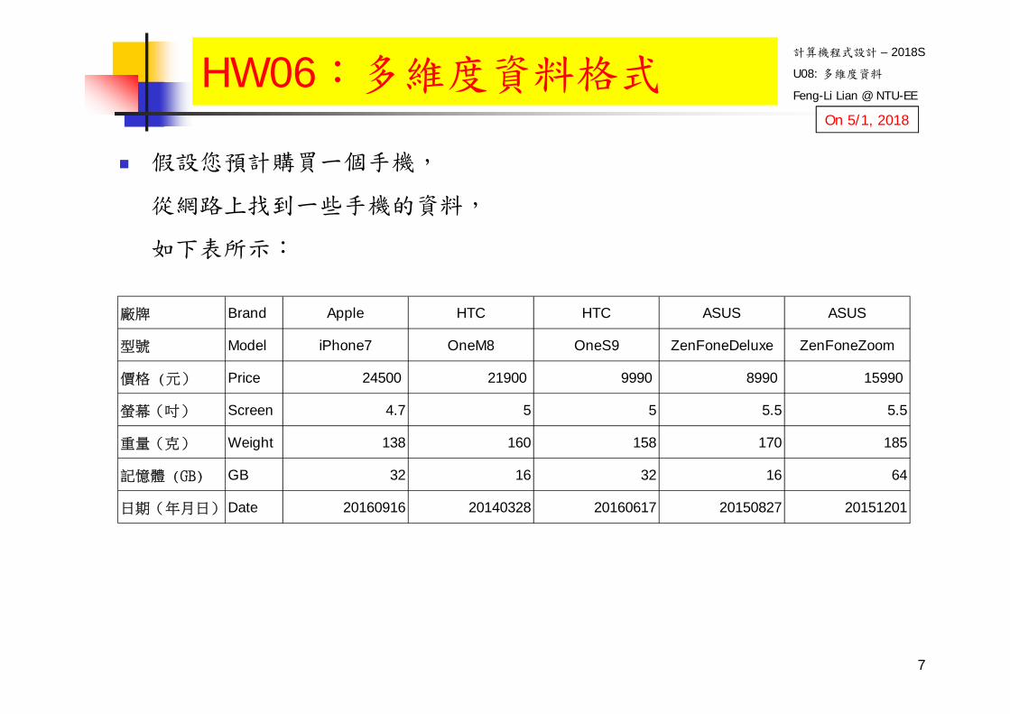
假設您預計購買一個手機，

從網路上找到一些手機的資料，

如下表所示：

廠牌 Brand Apple HTC HTC ASUS ASUS

型號 Model iPhone7 OneM8 OneS9 ZenFoneDeluxe ZenFoneZoom

價格 (元） Price 24500 21900 9990 8990 15990

螢幕（吋） Screen 4.7 5 5 5.5 5.5

重量（克） Weight 138 160 158 170 185

記憶體 (GB) GB 32 16 32 16 64

日期（年月日） Date 20160916 20140328 20160617 20150827 20151201

7

On 5/1, 2018




編輯一個程式於 .R 檔，完成下面的工作：

建立一個數列：Brand，放置五個手機的廠牌資料

建立一個數列：Model，放置五個手機的型號資料

建立一個數列：Price，放置五個手機的價格資料

建立一個數列：Screen，放置五個手機的螢幕資料

建立一個數列：Weight，放置五個手機的重量資料

建立一個數列：GB，放置五個手機的記憶體資料

建立一個數列：Date，放置五個手機的日期資料

建立一個 5x3 的矩陣 (matrix)：Number，放置五個手機的價格，螢幕，重量三種資料

建立一個資料框 (data.frame)：Phone，放置這五個手機的七種資料

建立一個資料框 (data.frame)：PhoneCheap，放置這五個手機，其價格小於10000元的手機的所有資料

您可以從一個一個數列慢慢建立起，也可以先建立一個資料框，再指定出個別的數列或矩陣

把執行的過程，以及產生的數據等，整理到報告檔 (pdf)。8

On 5/1, 2018




繳交下面檔案，檔案名稱：HW06_學號_關鍵字.xxx

主要指定檔案： HW06_B01921001_Phone.R 報告檔案： HW06_B01921001_Phone.pdf

繳交方式與期限：

E-mail 上面兩個檔案到：[email protected] E-mail 主旨：HW06_B01921001_Phone

(就是，作業編號_您的學號_關鍵字) 繳交期限：5/6 (Sun), 2018, 11pm 以前

學習方式：請至下面網址輸入此次的學習方式所花的時間：

https://goo.gl/k7tKLk https://docs.google.com/forms/d/e/1FAIpQLSdAZ_b-FUtvnNr_14rYQNYejMhDESy6jJ9ESh5XsjFI-DXMIw/viewform?c=0&w=1

9

On 5/1, 2018




矩陣 matrix 陣列 array 列表 list 資料框 data.frame 因子 factor

10




矩陣 – matrix

11




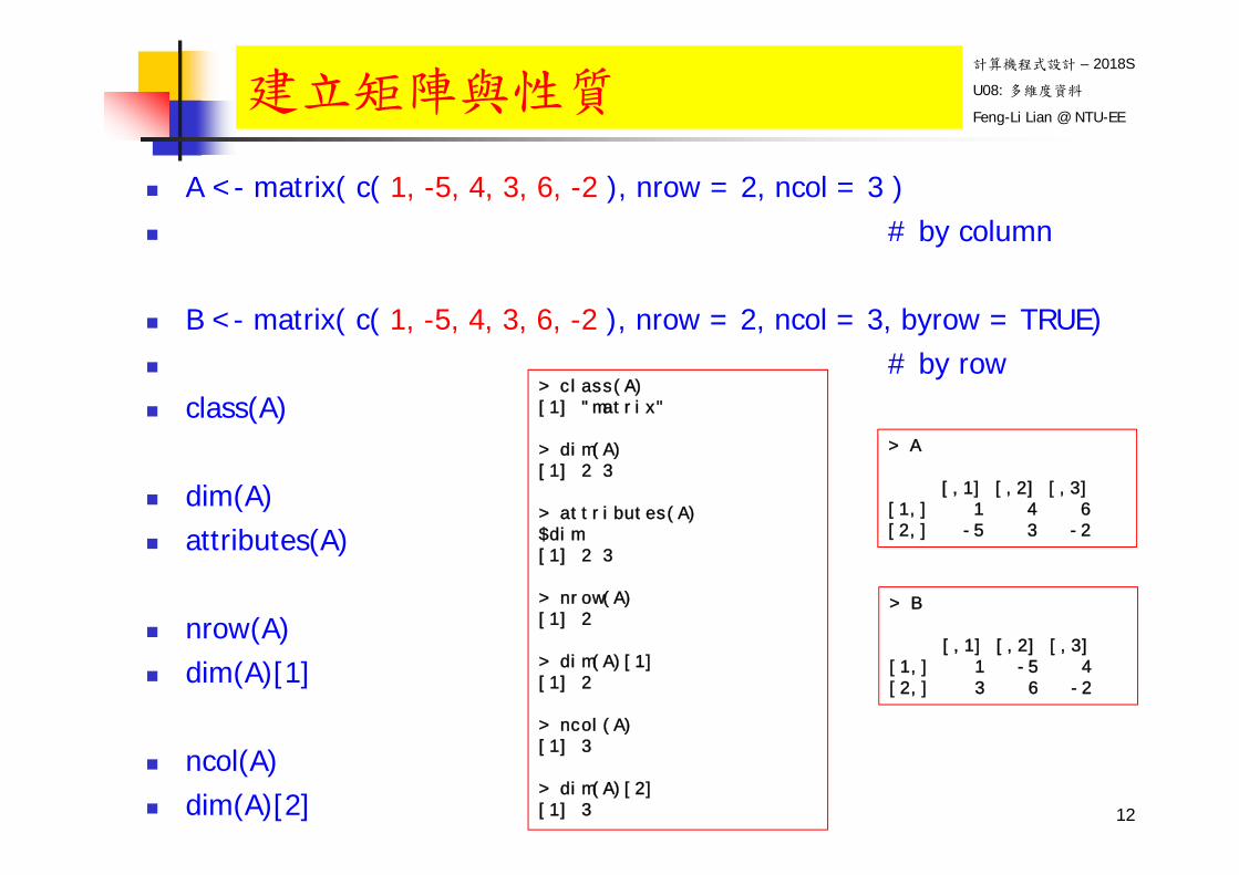
A <- matrix( c( 1, -5, 4, 3, 6, -2 ), nrow = 2, ncol = 3 ) # by column

B <- matrix( c( 1, -5, 4, 3, 6, -2 ), nrow = 2, ncol = 3, byrow = TRUE) # by row class(A)

dim(A) attributes(A)

nrow(A) dim(A)[1]

ncol(A) dim(A)[2]

建立矩陣與性質

12

> A

[,1] [,2] [,3][1,] 1 4 6[2,] -5 3 -2

> B

[,1] [,2] [,3][1,] 1 -5 4[2,] 3 6 -2

> class(A)[1] "matrix"

> dim(A)[1] 2 3

> attributes(A)$dim[1] 2 3

> nrow(A)[1] 2

> dim(A)[1][1] 2

> ncol(A)[1] 3

> dim(A)[2][1] 3




A <- matrix( c( 1, -5, 4, 3, 6, -2 ), nrow = 2, ncol = 3 )

u <- as.numeric(A)

v <- c(A)

dim(v)

length(v)

nrow(A) * ncol(A)

length(A)

矩陣與向量

13

> A[,1] [,2] [,3]

[1,] 1 4 6[2,] -5 3 -2

> u[1] 1 -5 4 3 6 -2

> v[1] 1 -5 4 3 6 -2

> dim(v)NULL

> length(v)[1] 6

> nrow(A) * ncol(A)[1] 6

> length(A)[1] 6




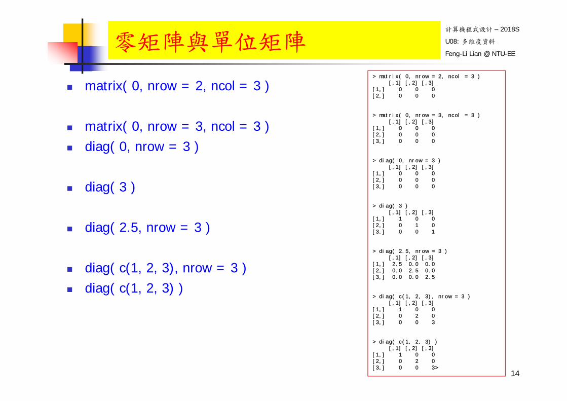
matrix( 0, nrow = 2, ncol = 3 )

matrix( 0, nrow = 3, ncol = 3 ) diag( 0, nrow = 3 )

diag( 3 )

diag( 2.5, nrow = 3 )

diag( c(1, 2, 3), nrow = 3 ) diag( c(1, 2, 3) )

零矩陣與單位矩陣

14

> matrix( 0, nrow = 2, ncol = 3 )[,1] [,2] [,3]

[1,] 0 0 0[2,] 0 0 0

> matrix( 0, nrow = 3, ncol = 3 )[,1] [,2] [,3]

[1,] 0 0 0[2,] 0 0 0[3,] 0 0 0

> diag( 0, nrow = 3 )[,1] [,2] [,3]

[1,] 0 0 0[2,] 0 0 0[3,] 0 0 0

> diag( 3 )[,1] [,2] [,3]

[1,] 1 0 0[2,] 0 1 0[3,] 0 0 1

> diag( 2.5, nrow = 3 )[,1] [,2] [,3]

[1,] 2.5 0.0 0.0[2,] 0.0 2.5 0.0[3,] 0.0 0.0 2.5

> diag( c(1, 2, 3), nrow = 3 )[,1] [,2] [,3]

[1,] 1 0 0[2,] 0 2 0[3,] 0 0 3

> diag( c(1, 2, 3) )[,1] [,2] [,3]

[1,] 1 0 0[2,] 0 2 0[3,] 0 0 3>




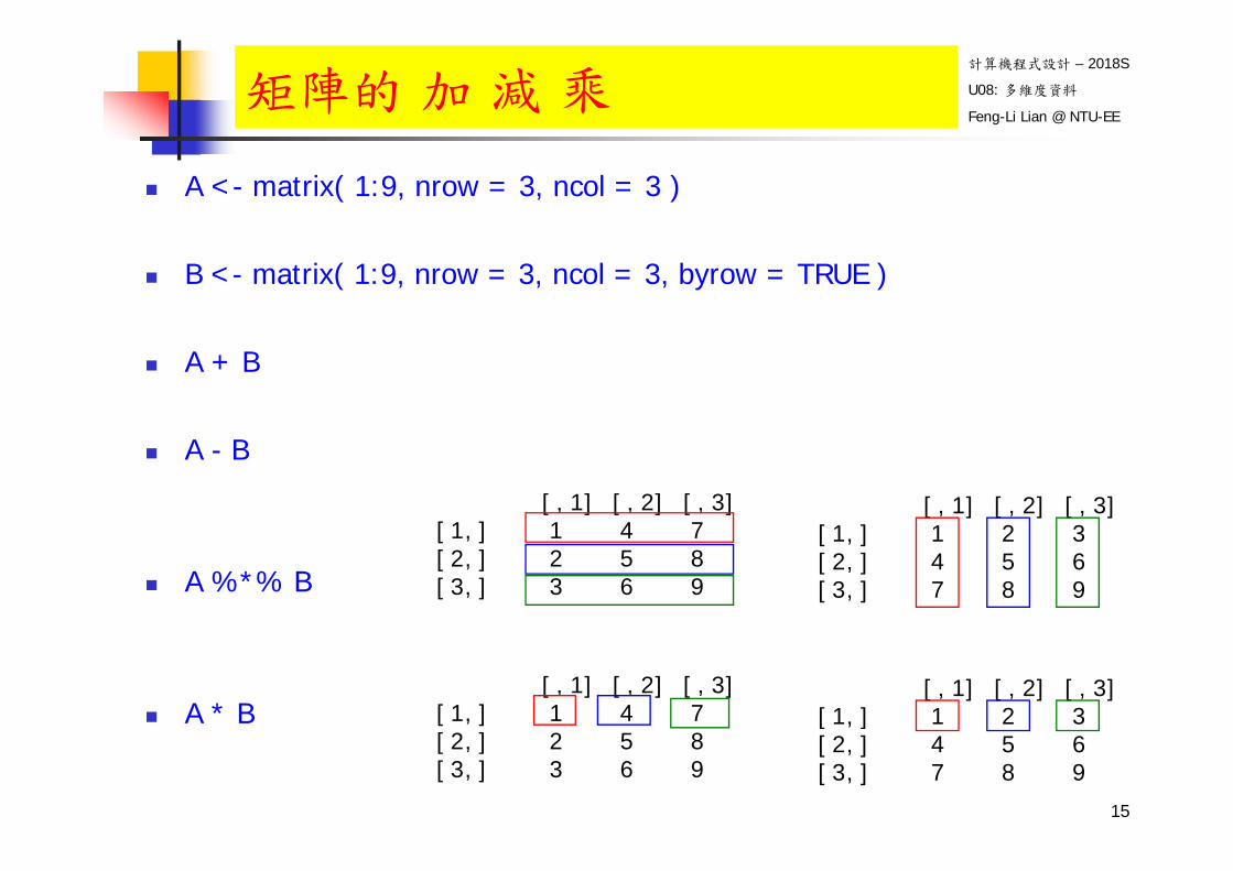
A <- matrix( 1:9, nrow = 3, ncol = 3 )

B <- matrix( 1:9, nrow = 3, ncol = 3, byrow = TRUE )

A + B

A - B

A %*% B

A * B

矩陣的加減乘

[,1] [,2] [,3][1,] 1 4 7[2,] 2 5 8[3,] 3 6 9

[,1] [,2] [,3][1,] 1 2 3[2,] 4 5 6[3,] 7 8 9

[,1] [,2] [,3][1,] 1 4 7[2,] 2 5 8[3,] 3 6 9

[,1] [,2] [,3][1,] 1 2 3[2,] 4 5 6[3,] 7 8 9

15




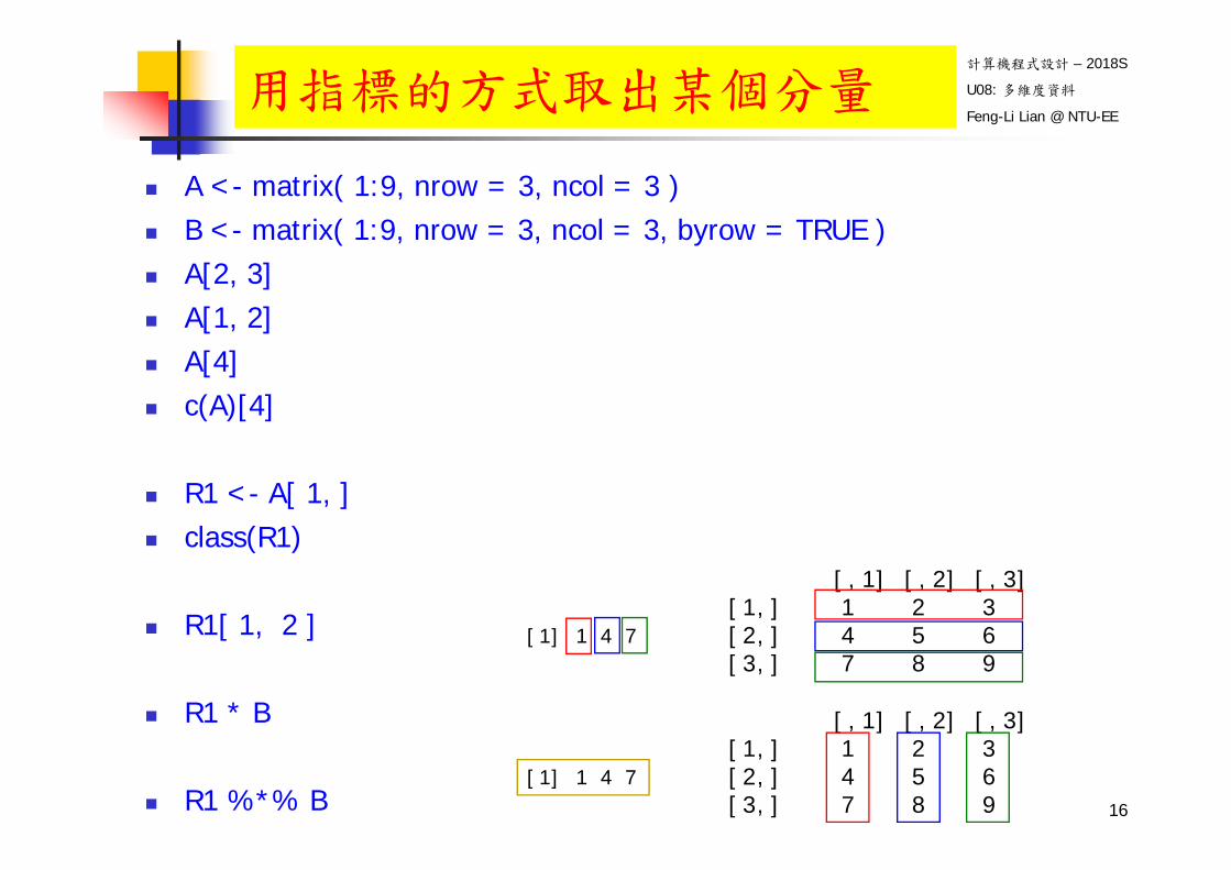
A <- matrix( 1:9, nrow = 3, ncol = 3 ) B <- matrix( 1:9, nrow = 3, ncol = 3, byrow = TRUE ) A[2, 3] A[1, 2] A[4] c(A)[4]

R1 <- A[ 1, ] class(R1)

R1[ 1, 2 ]

R1 * B

R1 %*% B

用指標的方式取出某個分量

[,1] [,2] [,3][1,] 1 2 3[2,] 4 5 6[3,] 7 8 9

[1] 1 4 7

[,1] [,2] [,3][1,] 1 2 3[2,] 4 5 6[3,] 7 8 9

[1] 1 4 7

16




A <- matrix( 1:9, nrow = 3, ncol = 3 ) B <- matrix( 1:9, nrow = 3, ncol = 3, byrow = TRUE )

R2 <- A[ 1, , drop = FALSE ] class( R2 )

R2[ 1, 2 ]

R2 %*% B

成為一個矩陣

17

> R1 <- A[ 1, ]

> class(R1)

[1] "integer"

> R2 <- A[ 1, , drop = FALSE ]

> class( R2 )

[1] "matrix"





E <- A[ c(1, 3), ]

class( E )

F <- A[ c(1, 3), 2 ]

class( F )

形成另外一個矩陣或向量

18

> E <- A[ c(1, 3), ]

> E[,1] [,2] [,3]

[1,] 1 4 7[2,] 3 6 9

> class( E )

[1] "matrix"

> F <- A[ c(1, 3), 2 ]

> F

[1] 4 6

> class( F )

[1] "integer"




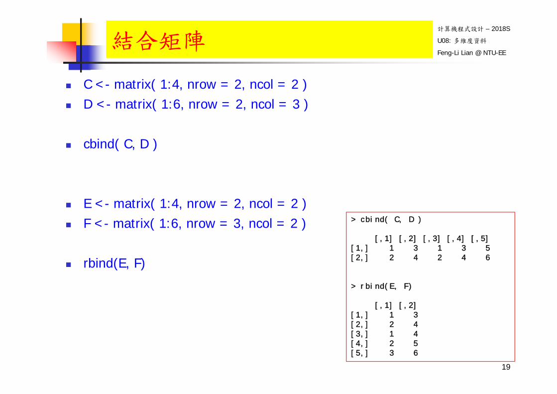
C <- matrix( 1:4, nrow = 2, ncol = 2 ) D <- matrix( 1:6, nrow = 2, ncol = 3 )

cbind( C, D )

E <- matrix( 1:4, nrow = 2, ncol = 2 ) F <- matrix( 1:6, nrow = 3, ncol = 2 )

rbind(E, F)

結合矩陣

19

> cbind( C, D )

[,1] [,2] [,3] [,4] [,5][1,] 1 3 1 3 5[2,] 2 4 2 4 6

> rbind(E, F)

[,1] [,2][1,] 1 3[2,] 2 4[3,] 1 4[4,] 2 5[5,] 3 6





t( A )

t( A ) %*% A

diag( A )

sum( diag( A ) )

轉置矩陣

20

> t( A )

[,1] [,2] [,3][1,] 1 2 3[2,] 4 5 6[3,] 7 8 9

> t( A ) %*% A

[,1] [,2] [,3][1,] 14 32 50[2,] 32 77 122[3,] 50 122 194

> diag( A )

[1] 1 5 9

> sum( diag( A ) )

[1] 15




A <- matrix( c(1, 0, 0, 3, 0.5, 0, 2, 1, 0.25), nrow = 3, ncol = 3 )

det(A)

Ainv <- solve(A)

Ainv

Ainv %*% A

矩陣的行列式值與反矩陣

A^(-1)

21

> det(A)

[1] 0.125

> Ainv <- solve(A)

> Ainv

[,1] [,2] [,3][1,] 1 -6 16[2,] 0 2 -8[3,] 0 0 4

> Ainv %*% A

[,1] [,2] [,3][1,] 1 0 0[2,] 0 1 0[3,] 0 0 1




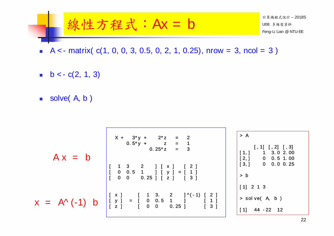
A <- matrix( c(1, 0, 0, 3, 0.5, 0, 2, 1, 0.25), nrow = 3, ncol = 3 )

b <- c(2, 1, 3)

solve( A, b )

線性方程式：Ax = b

A x = b

x = A^(-1) b

22

> A

[,1] [,2] [,3][1,] 1 3.0 2.00[2,] 0 0.5 1.00[3,] 0 0.0 0.25

> b

[1] 2 1 3

> solve( A, b )

[1] 44 -22 12

X + 3*y + 2*z = 20.5*y + z = 1

0.25*z = 3

[ 1 3 2 ] [ x ] [ 2 ][ 0 0.5 1 ] [ y ] = [ 1 ][ 0 0 0.25 ] [ z ] [ 3 ]

[ x ] [ 1 3. 2 ]^(-1) [ 2 ][ y ] = [ 0 0.5 1 ] [ 1 ][ z ] [ 0 0 0.25 ] [ 3 ]




陣列 – array

23




- 24

定義一個陣列

?array

array( data = NA, dim = length(data), dimnames = NULL )

data: 陣列內容的資料，預設值為 NA

dim: 維度，陣列的一個屬性

dimnames: 維度的名稱

array( 1:12 )

array( , c(3, 4) )

array( 1:12, c(3, 4) )

array( data = 1:12, dim = c(3, 4) )

array( data = 1:60, dim = c(3, 4, 5) )

args( array )

> array( 1:12 )

[1] 1 2 3 4 5 6 7 8 9 10 11 12

> array( , c(3, 4) )

[,1] [,2] [,3] [,4][1,] NA NA NA NA[2,] NA NA NA NA[3,] NA NA NA NA

> array( 1:12, c(3, 4) )

[,1] [,2] [,3] [,4][1,] 1 4 7 10[2,] 2 5 8 11[3,] 3 6 9 12

> array( data = 1:60, dim = c(3, 4, 5) )

, , 1

[,1] [,2] [,3] [,4][1,] 1 4 7 10[2,] 2 5 8 11[3,] 3 6 9 12

, , 2

[,1] [,2] [,3] [,4][1,] 13 16 19 22[2,] 14 17 20 23[3,] 15 18 21 24

, , 3………………………………………………………..




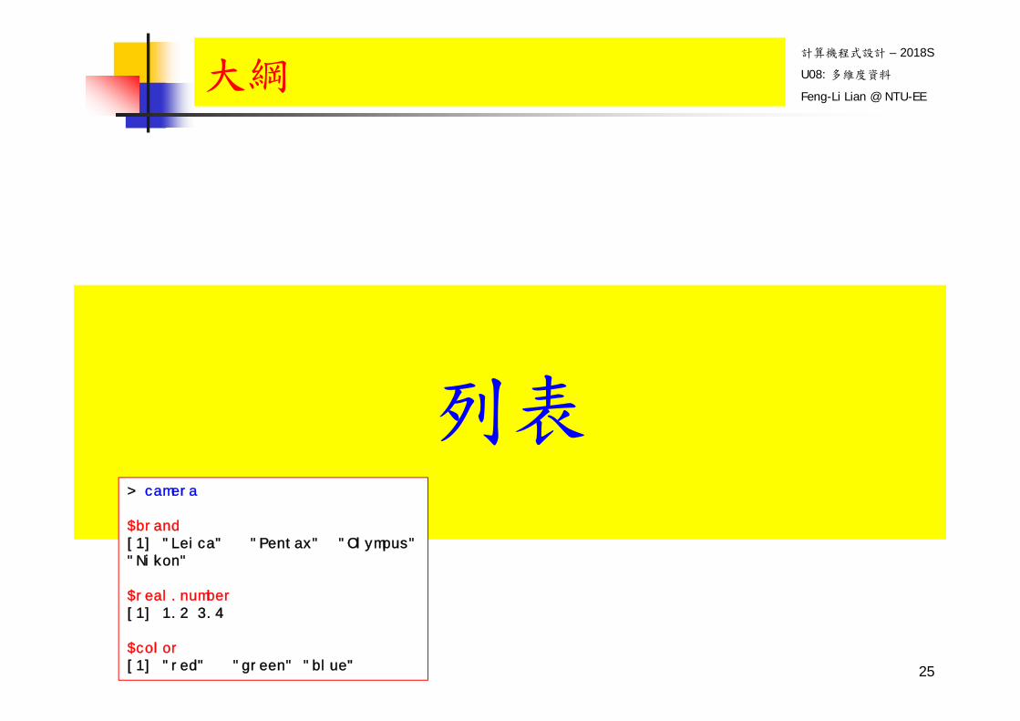
列表

25

> camera

$brand[1] "Leica" "Pentax" "Olympus" "Nikon"

$real.number[1] 1.2 3.4

$color[1] "red" "green" "blue"




camera <- list(c("Leica", "Pentax", "Olympus", "Nikon"), c(1.2, 3.4), c("red", "green", "blue"))

camera <-list( c("Leica", "Pentax", "Olympus", "Nikon"),

c(1.2, 3.4), c("red", "green", "blue")

)

camera <- list(brand = c("Leica", "Pentax", "Olympus", "Nikon"), real.number = c(1.2, 3.4), color = c("red", "green", "blue"))

camera <-list( brand = c("Leica", "Pentax", "Olympus", "Nikon"),

real.number = c(1.2, 3.4), color = c("red", "green", "blue")

)

列表

26

> camera

[[1]][1] "Leica" "Pentax" "Olympus" "Nikon"

[[2]][1] 1.2 3.4

[[3]][1] "red" "green" "blue"

> camera


$real.number[1] 1.2 3.4

$color[1] "red" "green" "blue"




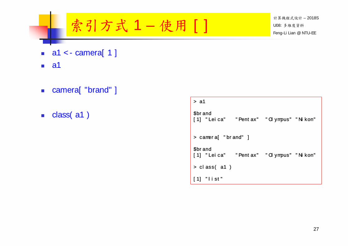
a1 <- camera[ 1 ] a1

camera[ "brand" ]

class( a1 )

索引方式 1 – 使用 [ ]

27

> a1


> camera[ "brand" ]


> class( a1 )

[1] "list"




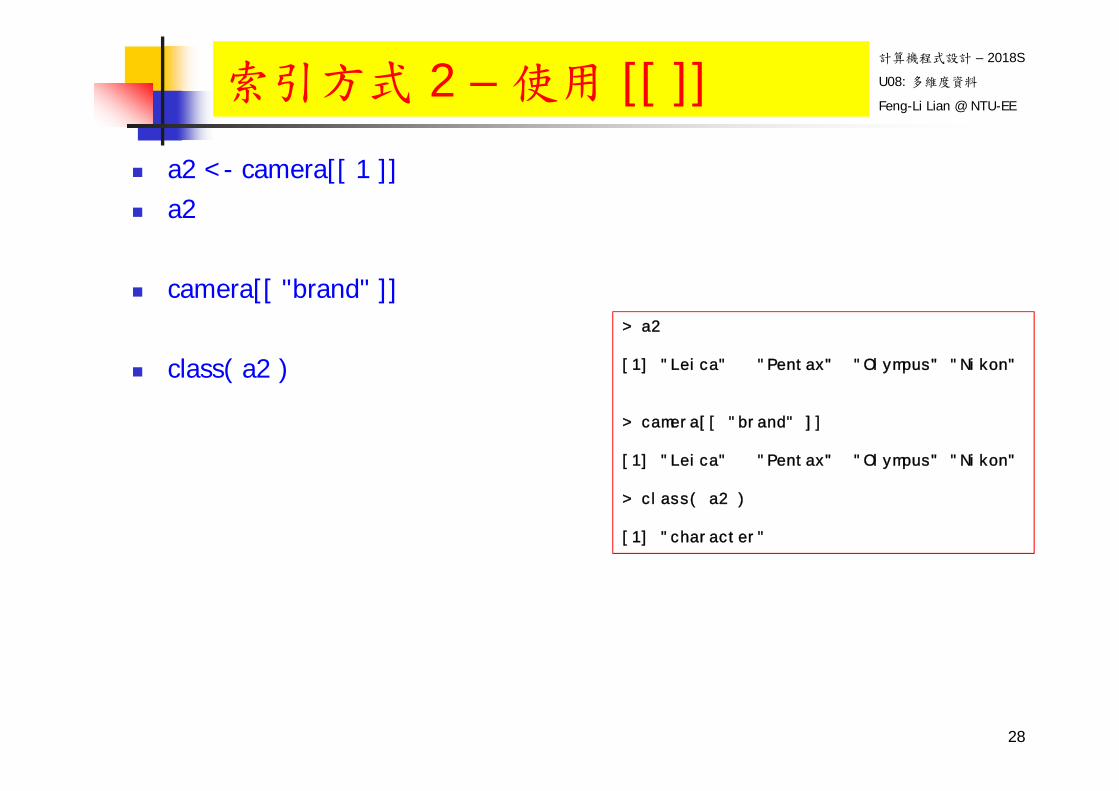
a2 <- camera[[ 1 ]] a2

camera[[ "brand" ]]

class( a2 )

索引方式 2 – 使用 [[ ]]

28

> a2

[1] "Leica" "Pentax" "Olympus" "Nikon"

> camera[[ "brand" ]]


> class( a2 )

[1] "character"




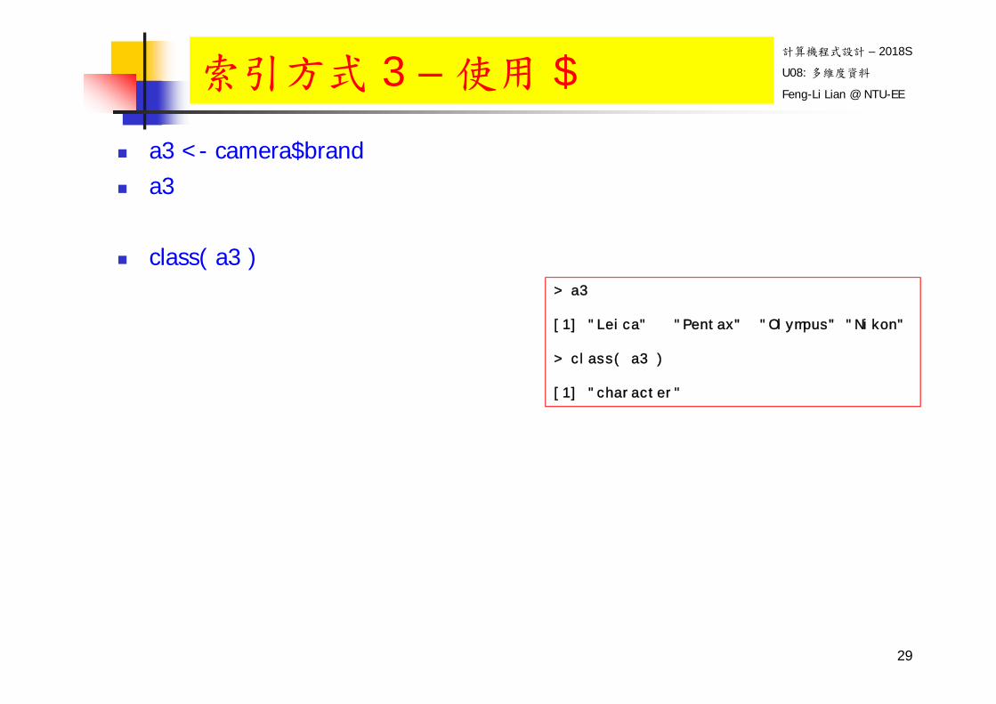
a3 <- camera$brand a3

class( a3 )

索引方式 3 – 使用 $

29

> a3


> class( a3 )

[1] "character"




a1 # a1 是列表

a2 # a2 是向量

a3 # a3 是向量

class( a1 ) class( a2 ) class( a3 )

camera[ 1 ][ 1 ] a1[ 1 ]

a2[ c(1, 2) ]

a3[ 2 ]

索引方式的比較

30

> a1 # a1 是列表$brand[1] "Leica" "Pentax" "Olympus" "Nikon"

> a2 # a2 是向量[1] "Leica" "Pentax" "Olympus" "Nikon"

> a3 # a3 是向量[1] "Leica" "Pentax" "Olympus" "Nikon"

> class( a1 )[1] "list"

> class( a2 )[1] "character"

> class( a3 )[1] "character"

> camera[ 1 ][ 1 ]$brand[1] "Leica" "Pentax" "Olympus" "Nikon"

> a1[ 1 ]$brand[1] "Leica" "Pentax" "Olympus" "Nikon"

> a2[ c(1, 2) ][1] "Leica" "Pentax"

> a3[ 2 ][1] "Pentax"




資料框

31

> camera

member brand color amount1 father Leica gold 22 mother Pentax red 13 brother Olympus green 14 sister Nikon blue 2




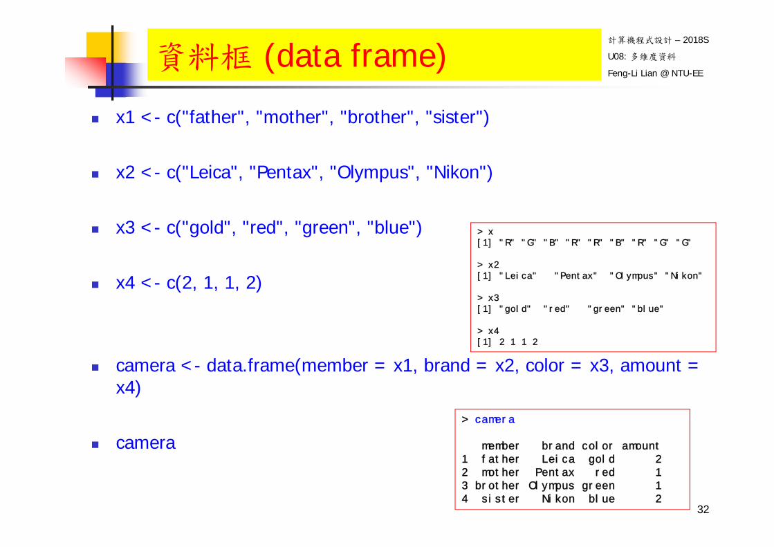
x1 <- c("father", "mother", "brother", "sister")

x2 <- c("Leica", "Pentax", "Olympus", "Nikon")

x3 <- c("gold", "red", "green", "blue")

x4 <- c(2, 1, 1, 2)

camera <- data.frame(member = x1, brand = x2, color = x3, amount = x4)

camera

資料框 (data frame)

32

> camera

member brand color amount1 father Leica gold 22 mother Pentax red 13 brother Olympus green 14 sister Nikon blue 2

> x[1] "R" "G" "B" "R" "R" "B" "R" "G" "G"

> x2[1] "Leica" "Pentax" "Olympus" "Nikon"

> x3[1] "gold" "red" "green" "blue"

> x4[1] 2 1 1 2




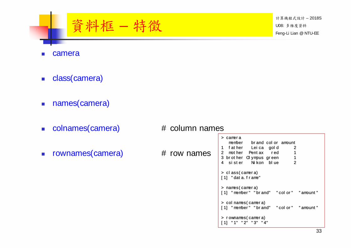
camera

class(camera)

names(camera)

colnames(camera) # column names

rownames(camera) # row names

資料框 – 特徵

33

> cameramember brand color amount

1 father Leica gold 22 mother Pentax red 13 brother Olympus green 14 sister Nikon blue 2

> class(camera)[1] "data.frame"

> names(camera)[1] "member" "brand" "color" "amount"

> colnames(camera) [1] "member" "brand" "color" "amount"

> rownames(camera) [1] "1" "2" "3" "4"




camera

camera$brand

camera[, 2]

camera[, "brand"]

資料框 – 內容

34

> cameramember brand color amount

1 father Leica gold 22 mother Pentax red 13 brother Olympus green 14 sister Nikon blue 2

> camera$brand[1] Leica Pentax Olympus Nikon Levels: Leica Nikon Olympus Pentax

> camera[, 2][1] Leica Pentax Olympus Nikon Levels: Leica Nikon Olympus Pentax

> camera[, "brand"][1] Leica Pentax Olympus Nikon Levels: Leica Nikon Olympus Pentax




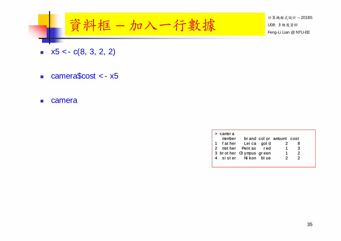
x5 <- c(8, 3, 2, 2)

camera$cost <- x5

camera

資料框 – 加入一行數據

35

> cameramember brand color amount cost

1 father Leica gold 2 82 mother Pentax red 1 33 brother Olympus green 1 24 sister Nikon blue 2 2




test <- camera

colnames(test)[c(4, 5)] <- c("number", "money")

test

資料框 – 改變名稱

36

> test

member brand color number money1 father Leica gold 2 82 mother Pentax red 1 33 brother Olympus green 1 24 sister Nikon blue 2 2




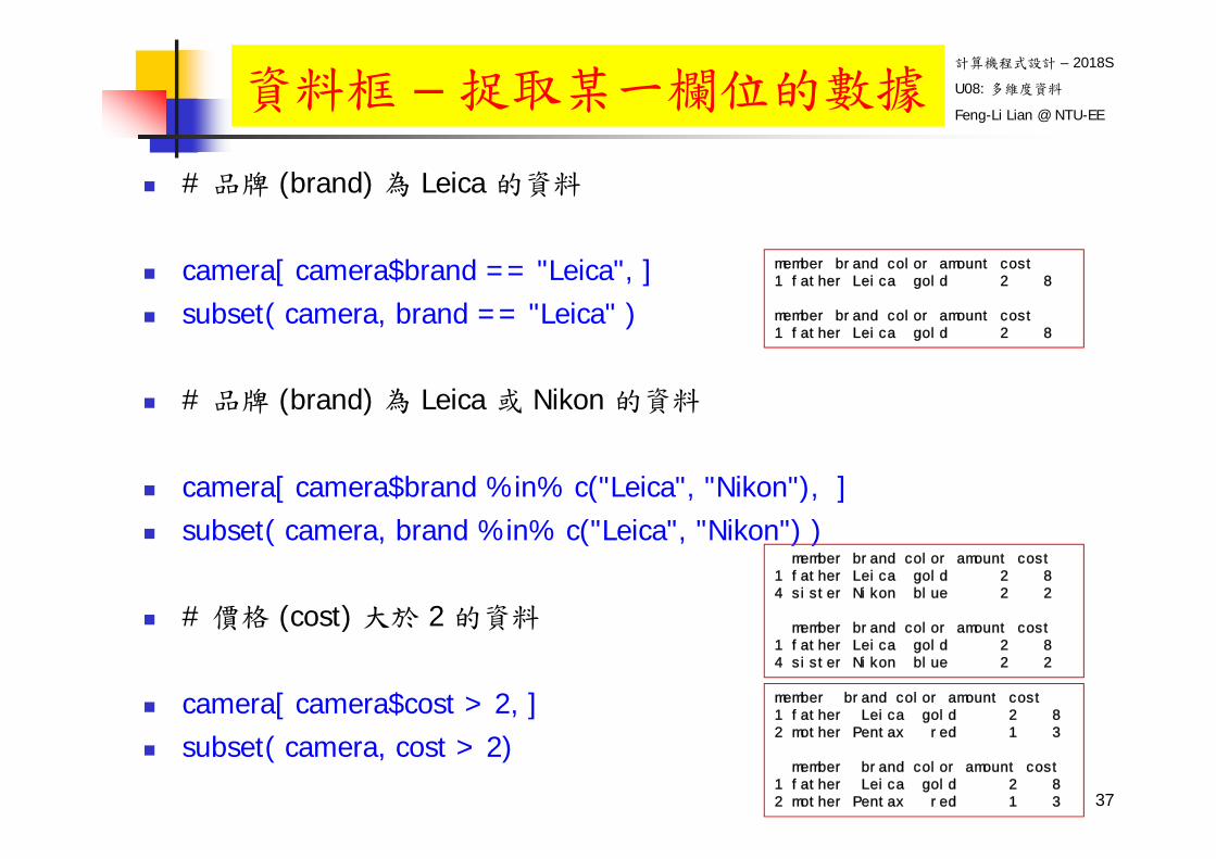
# 品牌 (brand) 為 Leica 的資料

camera[ camera$brand == "Leica", ] subset( camera, brand == "Leica" )

# 品牌 (brand) 為 Leica 或 Nikon 的資料

camera[ camera$brand %in% c("Leica", "Nikon"), ] subset( camera, brand %in% c("Leica", "Nikon") )

# 價格 (cost) 大於 2 的資料

camera[ camera$cost > 2, ] subset( camera, cost > 2)

資料框 – 捉取某一欄位的數據

37

member brand color amount cost1 father Leica gold 2 8

member brand color amount cost1 father Leica gold 2 8

member brand color amount cost1 father Leica gold 2 84 sister Nikon blue 2 2

member brand color amount cost1 father Leica gold 2 84 sister Nikon blue 2 2

member brand color amount cost1 father Leica gold 2 82 mother Pentax red 1 3

member brand color amount cost1 father Leica gold 2 82 mother Pentax red 1 3




A <- matrix( c(1, -5, 4, 3, 6, -2 ), nrow = 2, ncol = 3 )

rownames( A ) # row names colnames( A ) # column names

D <- as.data.frame( A )

names( D ) colnames( D ) rownames( D )

D$V1

資料框 – 把矩陣轉為資料框

38

> A[,1] [,2] [,3]

[1,] 1 4 6[2,] -5 3 -2

> rownames( A )NULL

> colnames( A )NULL

> D

V1 V2 V31 1 4 62 -5 3 -2

> names( D )[1] "V1" "V2" "V3"

> colnames( D )[1] "V1" "V2" "V3"

> rownames( D )[1] "1" "2"

> D$V1[1] 1 -5




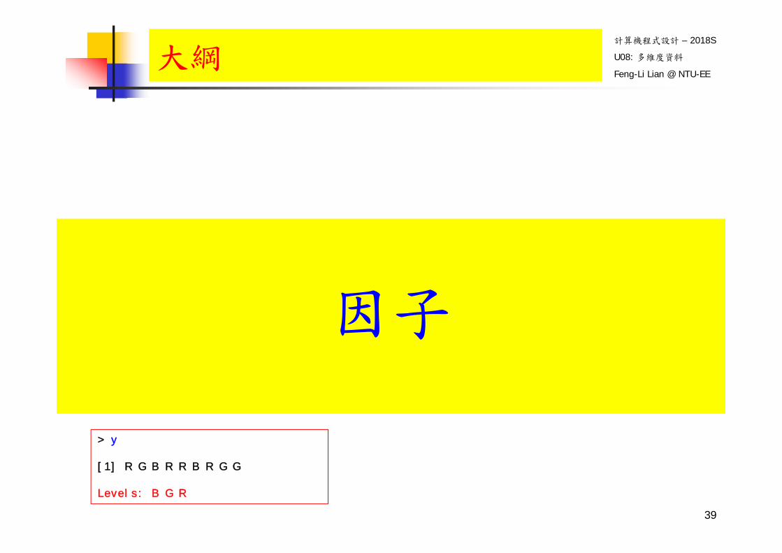
因子

39

> y

[1] R G B R R B R G G

Levels: B G R




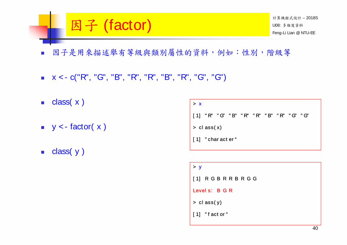
因子是用來描述舉有等級與類別屬性的資料，例如：性別，階級等

x <- c("R", "G", "B", "R", "R", "B", "R", "G", "G")

class( x )

y <- factor( x )

class( y )

因子 (factor)

40

> y

[1] R G B R R B R G G

Levels: B G R

> class(y)

[1] "factor"

> x

[1] "R" "G" "B" "R" "R" "B" "R" "G" "G"

> class(x)

[1] "character“




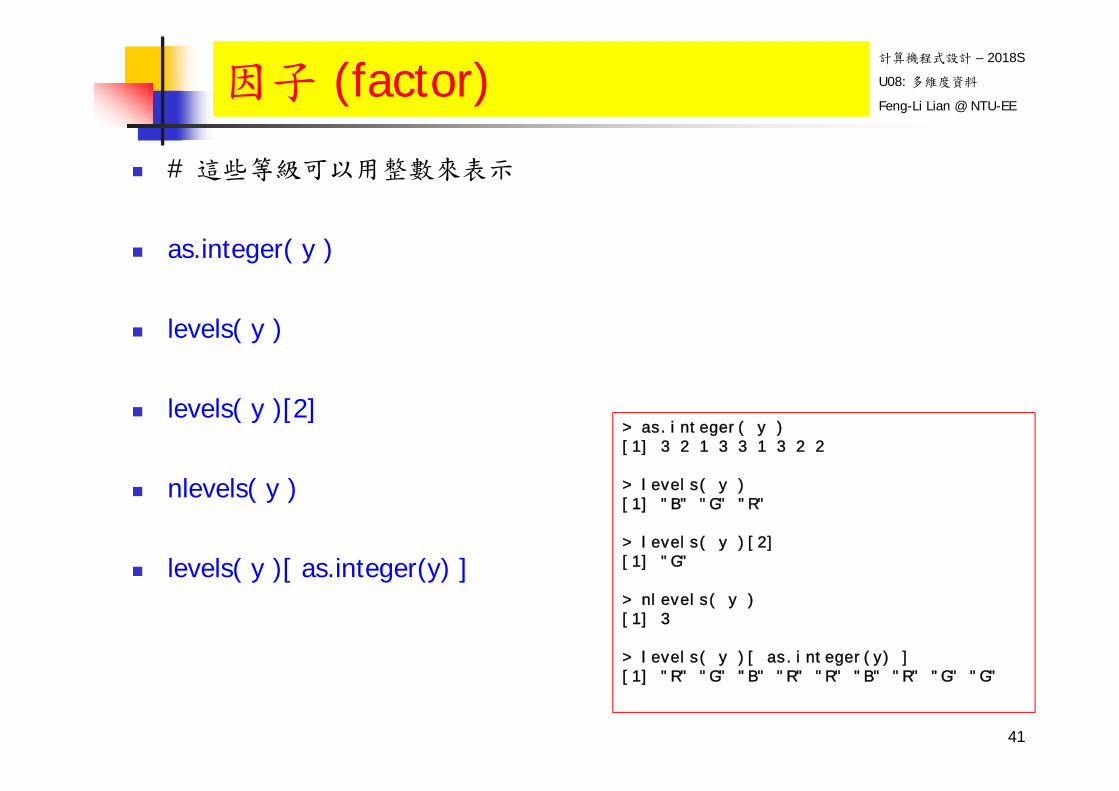
# 這些等級可以用整數來表示

as.integer( y )

levels( y )

levels( y )[2]

nlevels( y )

levels( y )[ as.integer(y) ]

因子 (factor)

41

> as.integer( y )[1] 3 2 1 3 3 1 3 2 2

> levels( y )[1] "B" "G" "R"

> levels( y )[2][1] "G"

> nlevels( y )[1] 3

> levels( y )[ as.integer(y) ][1] "R" "G" "B" "R" "R" "B" "R" "G" "G"




iris[,5] # iris[ , 5] - Levels: setosa versicolor virginica class( iris[ , 5 ] )

summary( iris )

class( CO2[ , 1 ] ) class( CO2[ , 2 ] ) class( CO2[ , 3 ] )

summary( CO2 )

因子案例 – iris, CO2

42

> iris[,5][1] setosa setosa setosa

…[56] versicolor versicolor versicolor

…[144] virginica virginica virginicavirginica virginica virginica virginicaLevels: setosa versicolor virginica

> class( iris[,5] )[1] "factor"

> class( CO2[,3] )[1] "factor"

> class( CO2[,2] )[1] "factor“

> class( CO2[,1] )[1] "ordered" "factor"

> CO2[,1][1] Qn1 Qn1 Qn1 Qn1 …… Mc3 Mc3 Mc3

Levels: Qn1 < Qn2 < Qn3 < Qc1 < Qc3 < Qc2 < Mn3 < Mn2 < Mn1 < Mc2 < Mc3 < Mc1

>




gl( 5, 3 ) # factor levels up to 5 with repeats of 3

gl( n = 5, k = 3 )

class( gl( 5, 3 ) )

gl( 5, 2, 13 )

gl( n = 5, k = 2, length = 13 )

is.factor( gl(5, 2, 13) )

產生因子 – 5的等級，3個分量

43

> gl( 5, 3 )

[1] 1 1 1 2 2 2 3 3 3 4 4 4 5 5 5Levels: 1 2 3 4 5

> gl( n = 5, k = 3 )

[1] 1 1 1 2 2 2 3 3 3 4 4 4 5 5 5Levels: 1 2 3 4 5

> class( gl( 5, 3 ) )

[1] "factor"

> gl( 5, 2, 13 )

[1] 1 1 2 2 3 3 4 4 5 5 1 1 2Levels: 1 2 3 4 5

> gl( n = 5, k = 2, length = 13 )

[1] 1 1 2 2 3 3 4 4 5 5 1 1 2Levels: 1 2 3 4 5

> is.factor( gl(5, 2, 13) )

[1] TRUE




下課了

44

106-2 cp08 多維度資料格式homepage.ntu.edu.tw/~fengli/Teaching/Computer/106-2_cp08.pdf ·...

Documents

Transcript of 106-2 cp08 多維度資料格式homepage.ntu.edu.tw/~fengli/Teaching/Computer/106-2_cp08.pdf ·...