NI PXI-1056 User Manual and Specifications - National Instruments
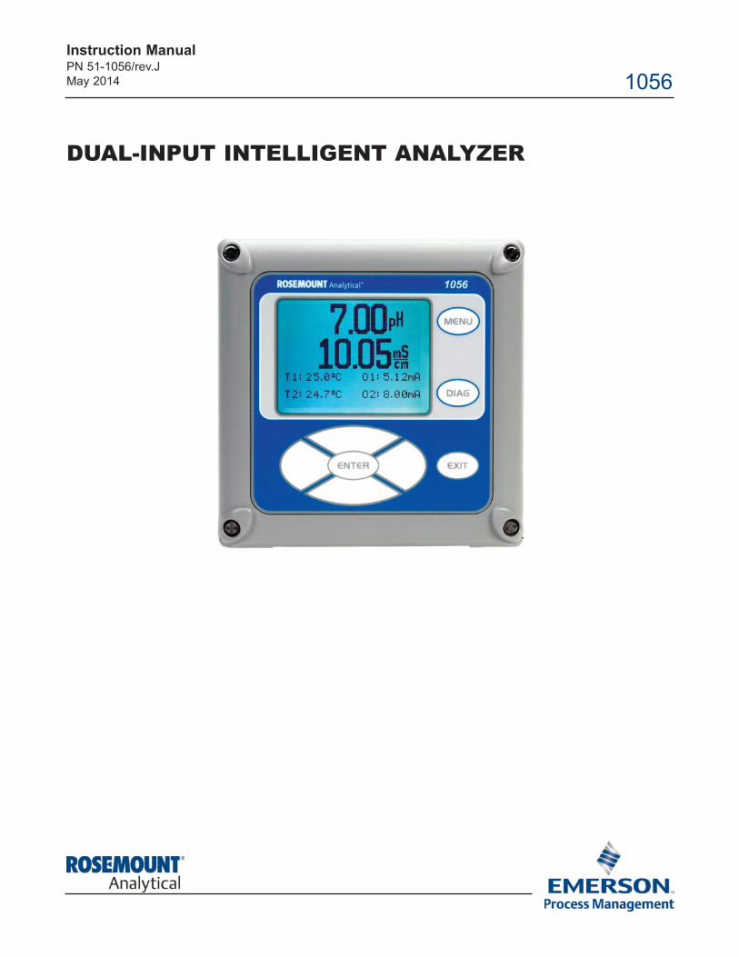
DUAL-INPUT INTELLIGENT ANALYZER
Instruction ManualPN 511056/rev.J
May 2014 1056
ESSENTIAL INSTRUCTIONS
READ THIS PAGE BEFORE PROCEEDING!
Your instrument purchase from Rosemount
Analytical, Inc. is one of the finest available for your
particular application. These instruments have been
designed, and tested to meet many national and
international standards. Experience indicates that its
performance is directly related to the quality of the
installation and knowledge of the user in operating
and maintaining the instrument. To ensure their con
tinued operation to the design specifications, per
sonnel should read this manual thoroughly before
proceeding with installation, commissioning, opera
tion, and maintenance of this instrument. If this
equipment is used in a manner not specified by the
manufacturer, the protection provided by it against
hazards may be impaired.
• Failure to follow the proper instructions may
cause any one of the following situations to
occur: Loss of life; personal injury; property dam
age; damage to this instrument; and warranty
invalidation.
• Ensure that you have received the correct model
and options from your purchase order. Verify that
this manual covers your model and options. If
not, call 18008548257 or 9497578500 to
request correct manual.
• For clarification of instructions, contact your
Rosemount representative.
• Follow all warnings, cautions, and instructions
marked on and supplied with the product.
• Use only qualified personnel to install, operate,
update, program and maintain the product.
• Educate your personnel in the proper installation,
operation, and maintenance of the product.
• Install equipment as specified in the Installation
section of this manual. Follow appropriate local
and national codes. Only connect the product to
electrical and pressure sources specified in this
manual.
• Use only factory documented components for
repair. Tampering or unauthorized substitution of
parts and procedures can affect the performance
and cause unsafe operation of your process.
• All equipment doors must be closed and protec
tive covers must be in place unless qualified per
sonnel are performing maintenance.
Equipment protected throughout by double insulation.
• Installation and servicing of this product may expose personelto dangerous voltages.
• Main power wired to separate power source must bedisconnected before servicing.
• Do not operate or energize instrument with case open!
• Signal wiring connected in this box must be rated at least 240 V.
• Nonmetallic cable strain reliefs do not provide grounding between conduit connections! Use grounding type bushings and jumper wires.
• Unused cable conduit entries must be securely sealed by nonflammable closures to provide enclosure integrity in compliance with personal safety and environmental protectionrequirements. Unused conduit openings must be sealed with NEMA 4X or IP65 conduit plugs to maintain the ingress protection rating (NEMA 4X).
• Electrical installation must be in accordance with the NationalElectrical Code (ANSI/NFPA70) and/or any other applicable national or local codes.
• Operate only with front panel fastened and in place.
• Safety and performance require that this instrument be connected and properly grounded through a threewire power source.
• Proper use and configuration is the responsibility of the
user.
This product generates, uses, and can radiate radio frequency
energy and thus can cause radio communication interference.
Improper installation, or operation, may increase such interfer
ence. As temporarily permitted by regulation, this unit has not
been tested for compliance within the limits of Class A comput
ing devices, pursuant to Subpart J of Part 15, of FCC Rules,
which are designed to provide reasonable protection against
such interference. Operation of this equipment in a residential
area may cause interference, in which case the user at his own
expense, will be required to take whatever measures may be
required to correct the interference.
This product is not intended for use in the light industrial,residential or commercial environments per the instrument’s certification to EN500812.
Emerson Process Management
2400 Barranca Parkway
Irvine, CA 92606 USA
Tel: (949) 7578500
Fax: (949) 4747250
http://www.rosemountanalytical.com
© Rosemount Analytical Inc. 2012
WARNINGRISK OF ELECTRICAL SHOCK
CAUTION
CAUTION
QUICK START GUIDE1056 Dual Input Analyzer
1. Refer to Section 2.0 for mechanical installation instructions.
2. Wire sensor(s) to the signal boards. See Section 3.0 for wiring instructions. Refer to the sensor instructionsheet for additional details. Make current output, alarm relay and power connections.
3. Once connections are secured and verified, apply power to the analyzer.
4. When the analyzer is powered up for the first time, Quick Start screens appear. Quick Start operating tipsare as follows:
a. A backlit field shows the position of the cursor.
b. To move the cursor left or right, use the keys to the left or right of the ENTER key. To scroll up or down or to increase or decrease the value of a digit use the keys above and below the ENTER key . Use the left or right keys to move the decimal point.
c. Press ENTER to store a setting. Press EXIT to leave without storing changes. Pressing EXIT during QuickStart returns the display to the initial startup screen (select language).
5. Complete the steps as shown in the Quick Start Guide flow diagram, Fig. A on the following page.
6. After the last step, the main display appears. The outputs are assigned to default values.
7. To change output, and temperaturerelated settings, go to the main menu and choose Program. Follow theprompts. For a general guide to the Program menu, see the Quick Reference Guide, Fig.B.
8. To return the analyzer to the default settings, choose Reset Analyzer under the Program menu.
Electrical installation must be in accordance withthe National Electrical Code (ANSI/NFPA70)and/or any other applicable national or local codes.
WARNINGRISK OF ELECTRICAL SHOCK
QU
ICK
STA
RT
GU
IDE
Fig
ure
A.
QU
ICK
STA
RT
GU
IDE
QU
ICK
RE
FE
RE
NC
E G
UID
EF
igu
re B
. M
OD
EL
1056 M
EN
U T
RE
E
This manual contains instructions for installation and operation of the Model 1056 DualInput IntelligentAnalyzer. The following list provides notes concerning all revisions of this document.
Rev. Level Date NotesA 01/07 This is the initial release of the product manual. The manual has been reformatted to reflect the
Emerson documentation style and updated to reflect any changes in the product offering.
B 2/07 Added CE mark to p.2. Replaced Quick Start Fig A.
C 9/07 Revised Sections 1,3,5,6, and 7. Added new measurements and features Turbidity, Flow, Current Input, Alarm relays and 4electrode conductivity.
D 11/07 Added 24VDC power supply to Sec. 3.4. Added CSA and FM agency approvals for option codes
01, 20, 21, 22, 24, 25, 26, 30, 31, 32, 34, 35, 36 and 38.
E 05/08 Add HART and Profibus DP digital communication to Section 1 specifications.
F 08/08 Updates
G 09/08 FM and CSA agency approval, Class 1, Div 2. for 24 VDC and AC switching power supplies.
H 04/10 Update DNV logo and company name
I 03/12 Update addresses mail and web
J 05/14 Update enclosure information
About This Document
MODEL 1056 TABLE OF CONTENTS
MODEL 1056
DUAL INPUT INTELLIGENT ANALYZER
TABLE OF CONTENTS
QUICK START GUIDE
QUICK REFERENCE GUIDE
TABLE OF CONTENTS
Section Title Page
1.0 DESCRIPTION AND SPECIFICATIONS ................................................................ 1
2.0 INSTALLATION ....................................................................................................... 11
2.1 Unpacking and Inspection........................................................................................ 11
2.2 Installation................................................................................................................ 11
3.0 WIRING.................................................................................................................... 19
3.1 General .................................................................................................................... 19
3.2 Preparing Conduit Openings.................................................................................... 19
3.3 Preparing Sensor Cable .......................................................................................... 20
3.4 Power, Output, Alarms and Sensor Connections..................................................... 20
4.0 DISPLAY AND OPERATION ................................................................................... 27
4.1 User Interface .......................................................................................................... 27
4.2 Instrument Keypad................................................................................................... 27
4.3 Main Display ............................................................................................................ 28
4.4 Menu System ........................................................................................................... 29
5.0 PROGRAMMING – BASICS ................................................................................... 31
5.1 General .................................................................................................................... 31
5.2 Changing the StartUp Settings ................................................................................ 31
5.3 Choosing Temperature units and Automatic/Manual Temperature Compensation .. 32
5.4 Configuring and Ranging the Current Outputs......................................................... 32
5.5 Setting a Security Code ........................................................................................... 34
5.6 Security Access........................................................................................................ 35
5.7 Using Hold ............................................................................................................... 35
5.8 Resetting Factory Defaults – Reset Analyzer .......................................................... 36
5.9 Alarm Relays............................................................................................................ 37
6.0 PROGRAMMING MEASUREMENTS ................................................................... 41
6.1 Programming Measurements – Introduction ........................................................... 41
6.2 pH ............................................................................................................................ 42
6.3 ORP ......................................................................................................................... 43
6.4 Contacting Conductivity .......................................................................................... 45
6.5 Toroidal Conductivity................................................................................................ 48
6.6 Chlorine.................................................................................................................... 51
6.6.1 Free Chlorine .................................................................................................. 51
6.6.2 Total Chlorine ................................................................................................. 53
6.6.3 Monochloramine ............................................................................................ 54
6.6.4 pHindependent Free Chlorine ....................................................................... 55
6.7 Oxygen..................................................................................................................... 57
6.8 Ozone ...................................................................................................................... 59
i
ii
MODEL 1056 TABLE OF CONTENTS
TABLE OF CONTENTS CONT’D
6.9 Turbidity ................................................................................................................... 60
6.10 Flow ......................................................................................................................... 63
6.11 Current Input ............................................................................................................ 64
7.0 CALIBRATION ...................................................................................................... 75
7.1 Calibration – Introduction ......................................................................................... 75
7.2 pH Calibration .......................................................................................................... 76
7.3 ORP Calibration ....................................................................................................... 78
7.4 Contacting Conductivity Calibration ......................................................................... 79
7.5 Toroidal Conductivity Calibration ............................................................................. 82
7.6 Chlorine Calibration ................................................................................................. 84
7.6.1 Free Chlorine .................................................................................................. 84
7.6.2 Total Chlorine .................................................................................................. 86
7.6.3 Monochloramine ............................................................................................. 88
7.6.4 pHIndependent Free Chlorine ....................................................................... 90
7.7 Oxygen Calibration .................................................................................................. 92
7.8 Ozone Calibration .................................................................................................... 95
7.9 Temperature Calibration........................................................................................... 97
7.10 Turbidity ................................................................................................................... 98
7.11 Pulse Flow ............................................................................................................... 100
8.0 RETURN OF MATERIAL ........................................................................................ 112
Warranty................................................................................................................... 112
MODEL 1056 TABLE OF CONTENTS
TABLE OF CONTENTS CONT’D
LIST OF FIGURES
Fig# Section Figure Title Page
A PREFACE Quick Start Guide
B PREFACE Quick Reference Guide
21 SEC 2.0 Panel Mounting Dimensions .............................................................. 12
22 SEC 2.0 Pipe and Wall Mounting Dimensions ................................................. 13
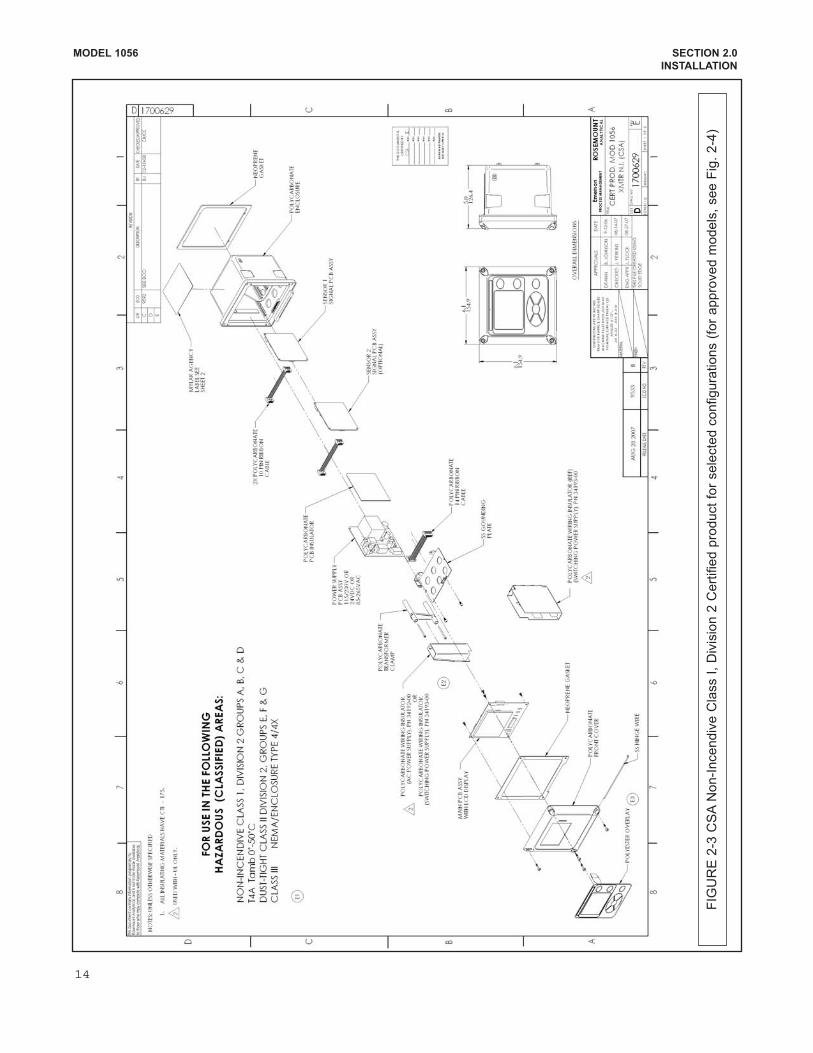
23 SEC 2.0 CSA Certification drawing part 1 ........................................................ 14
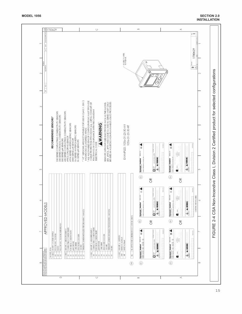
24 SEC 2.0 CSA Certification drawing part 2 ........................................................ 15
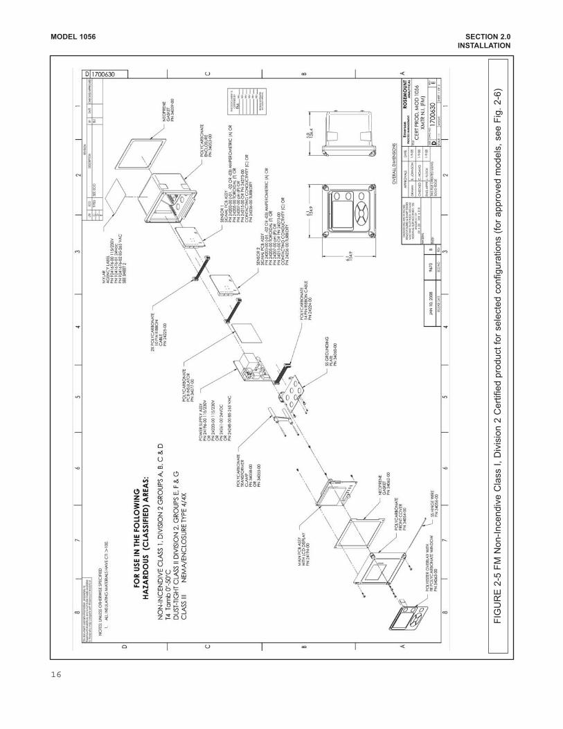
25 SEC 2.0 FM NonIncendive drawing part 1...................................................... 16
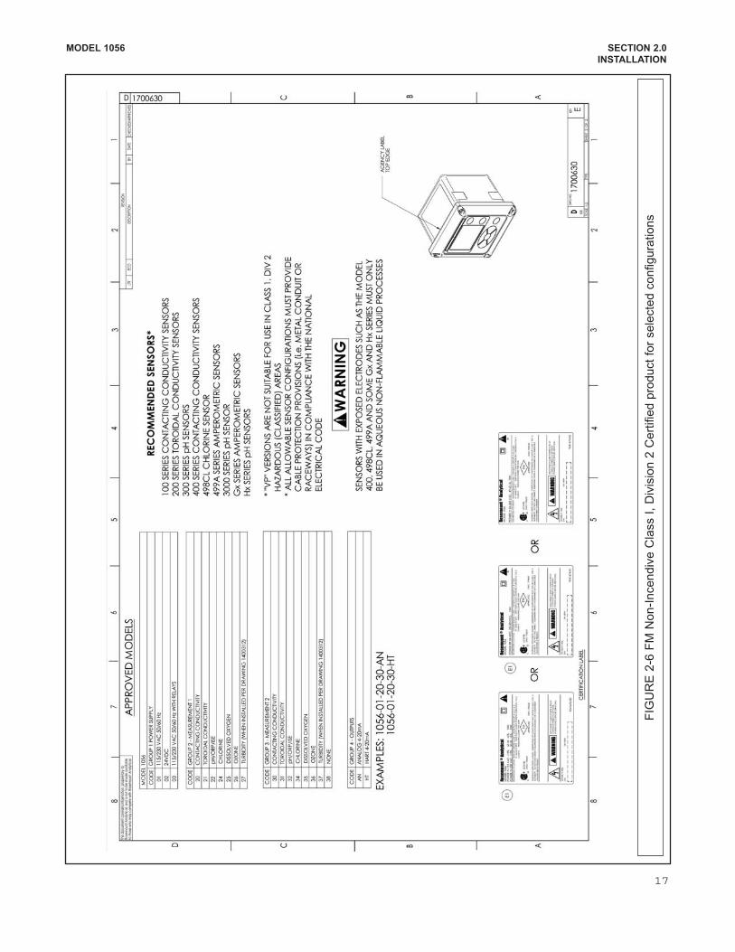
26 SEC 2.0 FM NonIncendive drawing part 2...................................................... 17
31 SEC 3.4 115/230 VAC Power Supply ............................................................... 20
32 SEC 3.4 24VDC Power Supply ........................................................................ 20
33 SEC 3.4 Switching AC Power Supply............................................................... 20
34 SEC 3.4 Current Output Wiring ........................................................................ 21
35 SEC 3.4 Alarm Relay Wiring for Model 1056 Switching Power Supply............ 21
36 SEC 3.4 Contacting Conductivity board and sensor cable leads ..................... 22
37 SEC 3.4 Toroidal Conductivity signal board and sensor cable leads ............... 22
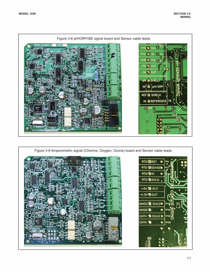
38 SEC 3.4 pH/ORP/ISE signal board and sensor cable leads ............................ 23
39 SEC 3.4 Amperometric board (Cl, O2, Ozone) and sensor cable leads .......... 23
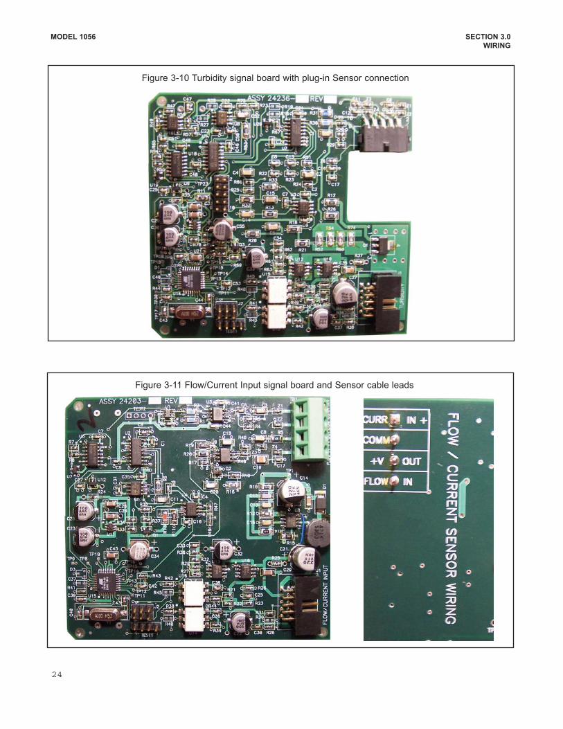
310 SEC 3.4 Turbidity signal board wiht plugin Sensor connection....................... 24
311 SEC 3.4 Flow/Current Input signal board and Sensor cable leads .................. 24
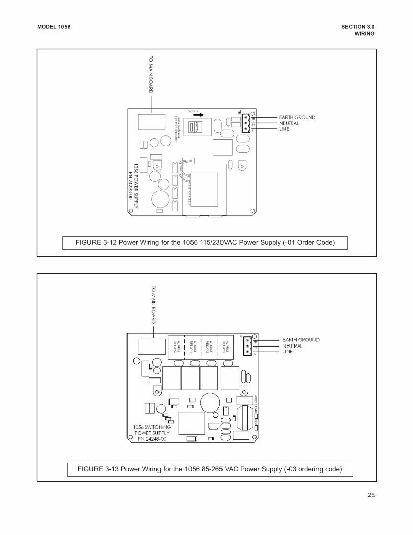
312 SEC 3.4 Power Wiring for Model 1056 115/230 VAC....................................... 25
313 SEC 3.4 Power Wiring for Model 1056 85265 VAC ........................................ 25
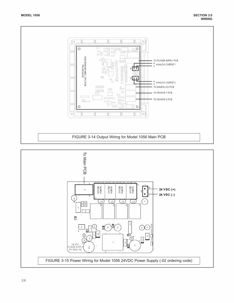
314 SEC 3.4 Output Wiring for Model 1056 Main PCB........................................... 26
315 SEC 3.4 Power Wiring for Model 1056 24VDC ................................................ 26
41 SEC 4.3 Formatting the Main Display ............................................................. 30
51 SEC 5.3.2 Choosing Temp Units and Manual Auto Temp Compensation ........... 32
52 SEC 5.4.5 Configuring and Ranging the Current Outputs................................... 33
53 SEC 5.5.2 Setting A Security Code .................................................................... 34
54 SEC 5.7.2 Using Hold ......................................................................................... 35
55 SEC 5.8.2 Resetting Factory Default Settings .................................................... 36
61 SEC 6.2 Configuring pH/ORP Measurements ................................................. 67
62 SEC 6.4 Configure Contacting Measurements ............................................... 68
63 SEC 6.5 Configure Toroidal Measurements .................................................... 69
64 SEC 6.6 Configure Chlorine Measurements .................................................... 71
65 SEC 6.7 Configure Oxygen Measurements ..................................................... 70
66 SEC 6.8 Configure Ozone Measurements ....................................................... 71
67 SEC 6.9 Configure Turbidity Measurement...................................................... 72
68 SEC 6.10 Configure Flow Measurement............................................................ 73
69 SEC 6.11 Configure mA Current Input Measurement........................................ 73
71 SEC 7.2 Calibrate pH ....................................................................................... 103
72 SEC 7.3 Calibrate ORP.................................................................................... 104
73 SEC 7.4 Calibrate Contacting and Toroidal Conductivity ................................. 105
74 SEC 7.6 Calibrate Chlorine .............................................................................. 106
75 SEC 7.7 Calibrate Oxygen ............................................................................... 107
76 SEC 7.8 Calibrate Ozone ................................................................................. 108
77 SEC 7.9 Calibrate Temperature ....................................................................... 109
78 SEC 7.10 Calibrate Turbidity .............................................................................. 110
79 SEC 7.11 Calibrate Flow.................................................................................... 111
iii
iv
MODEL 1056 TABLE OF CONTENTS
TABLE OF CONTENTS CONT’D
LIST OF TABLES
Number Section Table Title Page
51 SEC 5.2.1 Measurements and Measurement Units ............................................. 31
61 SEC 6.2.1 pH Measurement Programming ........................................................... 42
62 SEC 6.3.1 ORP Measurement Programming........................................................ 43
63 SEC 6.4.1 Contacting Conductivity Measurement Programming.......................... 45
64 SEC 6.5.1 Toroidal Conductivity Measurement Programming............................... 48
65 SEC 6.6.1.1 Free Chlorine Measurement Programming.......................................... 51
66 SEC 6.6.2.1 Total Chlorine Measurement Programming ......................................... 53
67 SEC 6.6.3.1Monochloramine Measurement Programming..................................... 54
68 SEC 6.6.4 pHIndependent Free Chlorine Measurement Programming ............ 55
69 SEC. 6.7.1 Oxygen Measurement Programming.................................................... 57
610 SEC 6.8.1 Ozone Measurement Programming...................................................... 59
611 SEC 6.9.1 Turbidity Measurement Programming.................................................. 60
612 SEC 6.10.1 Flow Measurement Programming......................................................... 63
613 SEC 6.11.1 Curent Input Programming................................................................... 64
71 SEC 7.2 pH Calibration Routines ....................................................................... 76
72 SEC 7.3 ORP Calibration Routine...................................................................... 78
73 SEC 7.4 Contacting Conductivity Calibration Routines...................................... 79
74 SEC 7.5 Toroidal Conductivity Calibration ........................................... ............ 82
75 SEC 7.6.1 Free Chlorine Calibration Routines....................................................... 85
76 SEC 7.6.2 Total Chlorine Calibration Routines...................................................... 86
77 SEC 7.6.3 Monochloramine Calibration Routines.................................................. 88
78 SEC 7.6.4 pHindependent Free Chlorine Calibration Routines............................ 90
79 SEC 7.7 Oxygen Calibration Routines................................................................ 93
710 SEC 7.8 Ozone Calibration Routines.................................................................. 95
711 SEC 7.9 Temperature Calibration Routines........................................................ 97
712 SEC 7.10 Turbidity Calibration Routines............................................................... 98
713 SEC 7.11 Flow Calibration Routines................................................................... 100
SECTION 1.0.
DESCRIPTION AND SPECIFICATIONS
1
MODEL 1056 SECTION 1.0
DESCRIPTION AND SPECIFICATIONS
FEATURES AND APPLICATIONS
The 1056 dualinput analyzer offers single or dual sensor input with an unrestricted choice of dual measurements. This multiparameter instrument offers a widerange of measurement choices supporting most industrial, commercial, and municipal applications. Themodular design allows signal input boards to be fieldreplaced making configuration changes easy.Conveniently, live process values are always displayedduring programming and calibration routines.
QUICK START PROGRAMMING: Exclusive QuickStart screens appear the first time the 1056 is powered. The instrument autorecognizes each measurement board and prompts the user to configure eachsensor loop in a few quick steps for immediate deployment.
DIGITAL COMMUNICATIONS: HART and ProfibusDP digital communications are available. The 1056HART units communicate with the Model 375 HART®
handheld communicator and HART hosts, such asAMS Intelligent Device Manager. Model 1056 Profibusunits are fully compatible with Profibus DP networksand Class 1 or Class 2 masters. HART and ProfibusDP configured units will support any single or dualmeasurement configuration of Model 1056.
MENUS: Menu screens for calibrating and programmingare simple and intuitive. Plain language prompts andhelp screens guide the user through these procedures.
DUAL SENSOR INPUT AND OUTPUT: The 1056accepts single or dual sensor input. Standard 0/420 mA current outputs can be programmed tocorrespond to any measurement or temperature.
ENCLOSURE: The instrument fits standard ½ DINpanel cutouts. The versatile enclosure design supportspanelmount, pipemount, and surface/wallmountinstallations.
ISOLATED INPUTS: Inputs are isolated from othersignal sources and earth ground. This ensures cleansignal inputs for single and dual input configurations.For dual input configurations, isolation allows anycombination of measurements and signal inputs without crosstalk or signal interference.
TEMPERATURE: Most measurements require temperature compensation. The 1056 will automaticallyrecognize Pt100, Pt1000 or 22k NTC RTDs built intothe sensor.
SECURITY ACCESS CODES: Two levels of securityaccess are available. Program one access code forroutine calibration and hold of current outputs; programanother access code for all menus and functions.
• MULTIPARAMETER INSTRUMENT – single or dual input. Choose from pH/ORP/ISE,
Resistivity/Conductivity, % Concentration, Chlorine, Oxygen, Ozone, Temperature, Turbidity, Flow,
and 420mA Current Input.
• LARGE DISPLAY – large easytoread process measurements.
• EASY TO INSTALL – modular boards, removable connectors, easy to wire power, sensors, and outputs.
• INTUITIVE MENU SCREENS with advanced diagnostics and help screens.
• SEVEN LANGUAGES included: English, French, German, Italian, Spanish, Portuguese, and Chinese.
• HART® AND PROFIBUS® DP Digital Communications options
MODEL 1056 SECTION 1.0
DESCRIPTION AND SPECIFICATIONS
2
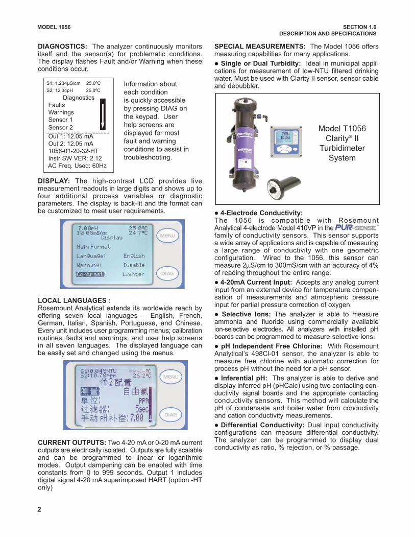
DIAGNOSTICS: The analyzer continuously monitorsitself and the sensor(s) for problematic conditions.The display flashes Fault and/or Warning when theseconditions occur.
DISPLAY: The highcontrast LCD provides livemeasurement readouts in large digits and shows up tofour additional process variables or diagnosticparameters. The display is backlit and the format canbe customized to meet user requirements.
LOCAL LANGUAGES :Rosemount Analytical extends its worldwide reach byoffering seven local languages – English, French,German, Italian, Spanish, Portuguese, and Chinese.Every unit includes user programming menus; calibrationroutines; faults and warnings; and user help screensin all seven languages. The displayed language canbe easily set and changed using the menus.
CURRENT OUTPUTS: Two 420 mA or 020 mA currentoutputs are electrically isolated. Outputs are fully scalableand can be programmed to linear or logarithmicmodes. Output dampening can be enabled with timeconstants from 0 to 999 seconds. Output 1 includesdigital signal 420 mA superimposed HART (option HTonly)
SPECIAL MEASUREMENTS: The Model 1056 offersmeasuring capabilities for many applications.
l Single or Dual Turbidity: Ideal in municipal applications for measurement of lowNTU filtered drinkingwater. Must be used with Clarity II sensor, sensor cableand debubbler.
l 4Electrode Conductivity:The 1056 is compat ib le wi th RosemountAnalytical 4electrode Model 410VP in the PURSENSE family of conductivity sensors. This sensor supportsa wide array of applications and is capable of measuringa large range of conductivity with one geometricconfiguration. Wired to the 1056, this sensor canmeasure 2μS/cm to 300mS/cm with an accuracy of 4%of reading throughout the entire range.
l 420mA Current Input: Accepts any analog currentinput from an external device for temperature compensation of measurements and atmospheric pressureinput for partial pressure correction of oxygen.
l Selective Ions: The analyzer is able to measureammonia and fluoride using commercially availableionselective electrodes. All analyzers with installed pHboards can be programmed to measure selective ions.
l pH Independent Free Chlorine: With RosemountAnalytical’s 498Cl01 sensor, the analyzer is able tomeasure free chlorine with automatic correction forprocess pH without the need for a pH sensor.
l Inferential pH: The analyzer is able to derive anddisplay inferred pH (pHCalc) using two contacting conductivity signal boards and the appropriate contactingconductivity sensors. This method will calculate thepH of condensate and boiler water from conductivityand cation conductivity measurements.
l Differential Conductivity: Dual input conductivityconfigurations can measure differential conductivity.The analyzer can be programmed to display dualconductivity as ratio, % rejection, or % passage.
S1: 1.234µS/cm 25.0ºC
S2: 12.34pH 25.0ºC
Diagnostics
Faults
Warnings
Sensor 1
Sensor 2
Out 1: 12.05 mA
Out 2: 12.05 mA
1056012032HT
Instr SW VER: 2.12
AC Freq. Used: 60Hz
Information about
each condition
is quickly accessible
by pressing DIAG on
the keypad. User
help screens are
displayed for most
fault and warning
conditions to assist in
troubleshooting.
Model T1056
Clarity® II
Turbidimeter
System
MODEL 1056 SECTION 1.0
DESCRIPTION AND SPECIFICATIONS
3
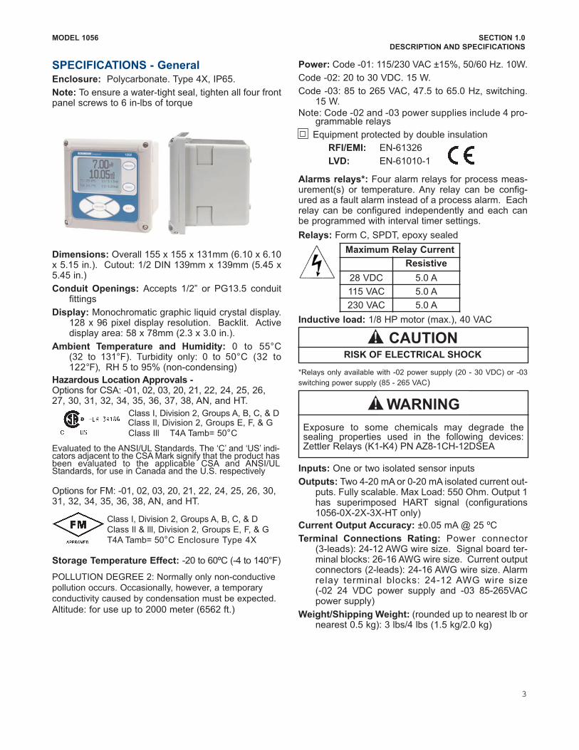
SPECIFICATIONS GeneralEnclosure: Polycarbonate. Type 4X, IP65.
Note: To ensure a watertight seal, tighten all four frontpanel screws to 6 inlbs of torque
Dimensions: Overall 155 x 155 x 131mm (6.10 x 6.10x 5.15 in.). Cutout: 1/2 DIN 139mm x 139mm (5.45 x5.45 in.)
Conduit Openings: Accepts 1/2” or PG13.5 conduitfittings
Display: Monochromatic graphic liquid crystal display.128 x 96 pixel display resolution. Backlit. Activedisplay area: 58 x 78mm (2.3 x 3.0 in.).
Ambient Temperature and Humidity: 0 to 55°C(32 to 131°F). Turbidity only: 0 to 50°C (32 to122°F), RH 5 to 95% (noncondensing)
Storage Temperature Effect: 20 to 60ºC (4 to 140°F)
Power: Code 01: 115/230 VAC ±15%, 50/60 Hz. 10W.
Code 02: 20 to 30 VDC. 15 W.
Code 03: 85 to 265 VAC, 47.5 to 65.0 Hz, switching.15 W.
Note: Code 02 and 03 power supplies include 4 programmable relays
Equipment protected by double insulation
Alarms relays*: Four alarm relays for process measurement(s) or temperature. Any relay can be configured as a fault alarm instead of a process alarm. Eachrelay can be configured independently and each canbe programmed with interval timer settings.
Relays: Form C, SPDT, epoxy sealed
Inductive load: 1/8 HP motor (max.), 40 VAC
*Relays only available with 02 power supply (20 30 VDC) or 03
switching power supply (85 265 VAC)
Inputs: One or two isolated sensor inputs
Outputs: Two 420 mA or 020 mA isolated current outputs. Fully scalable. Max Load: 550 Ohm. Output 1has superimposed HART signal (configurations10560X2X3XHT only)
Current Output Accuracy: ±0.05 mA @ 25 ºC
Terminal Connections Rating: Power connector(3leads): 2412 AWG wire size. Signal board terminal blocks: 2616 AWG wire size. Current outputconnectors (2leads): 2416 AWG wire size. Alarmrelay terminal blocks: 2412 AWG wire size(02 24 VDC power supply and 03 85265VACpower supply)
Weight/Shipping Weight: (rounded up to nearest lb ornearest 0.5 kg): 3 lbs/4 lbs (1.5 kg/2.0 kg)
RFI/EMI: EN61326
LVD: EN610101
Hazardous Location Approvals Options for CSA: 01, 02, 03, 20, 21, 22, 24, 25, 26,27, 30, 31, 32, 34, 35, 36, 37, 38, AN, and HT.
Class I, Division 2, Groups A, B, C, & DClass Il, Division 2, Groups E, F, & G
Class Ill T4A Tamb= 50°C
Evaluated to the ANSI/UL Standards. The ‘C’ and ‘US’ indicators adjacent to the CSA Mark signify that the product hasbeen evaluated to the applicable CSA and ANSI/ULStandards, for use in Canada and the U.S. respectively
Class I, Division 2, Groups A, B, C, & D
Class Il & lll, Division 2, Groups E, F, & G
T4A Tamb= 50°C Enclosure Type 4X
CAUTIONRISK OF ELECTRICAL SHOCK
Maximum Relay Current
Resistive
28 VDC 5.0 A
115 VAC 5.0 A
230 VAC 5.0 A
POLLUTION DEGREE 2: Normally only nonconductive
pollution occurs. Occasionally, however, a temporary
conductivity caused by condensation must be expected.
Altitude: for use up to 2000 meter (6562 ft.)
WARNING
Exposure to some chemicals may degrade thesealing properties used in the following devices:Zettler Relays (K1K4) PN AZ81CH12DSEA
WARNING
Options for FM: 01, 02, 03, 20, 21, 22, 24, 25, 26, 30,31, 32, 34, 35, 36, 38, AN, and HT.
MODEL 1056 SECTION 1.0
DESCRIPTION AND SPECIFICATIONS
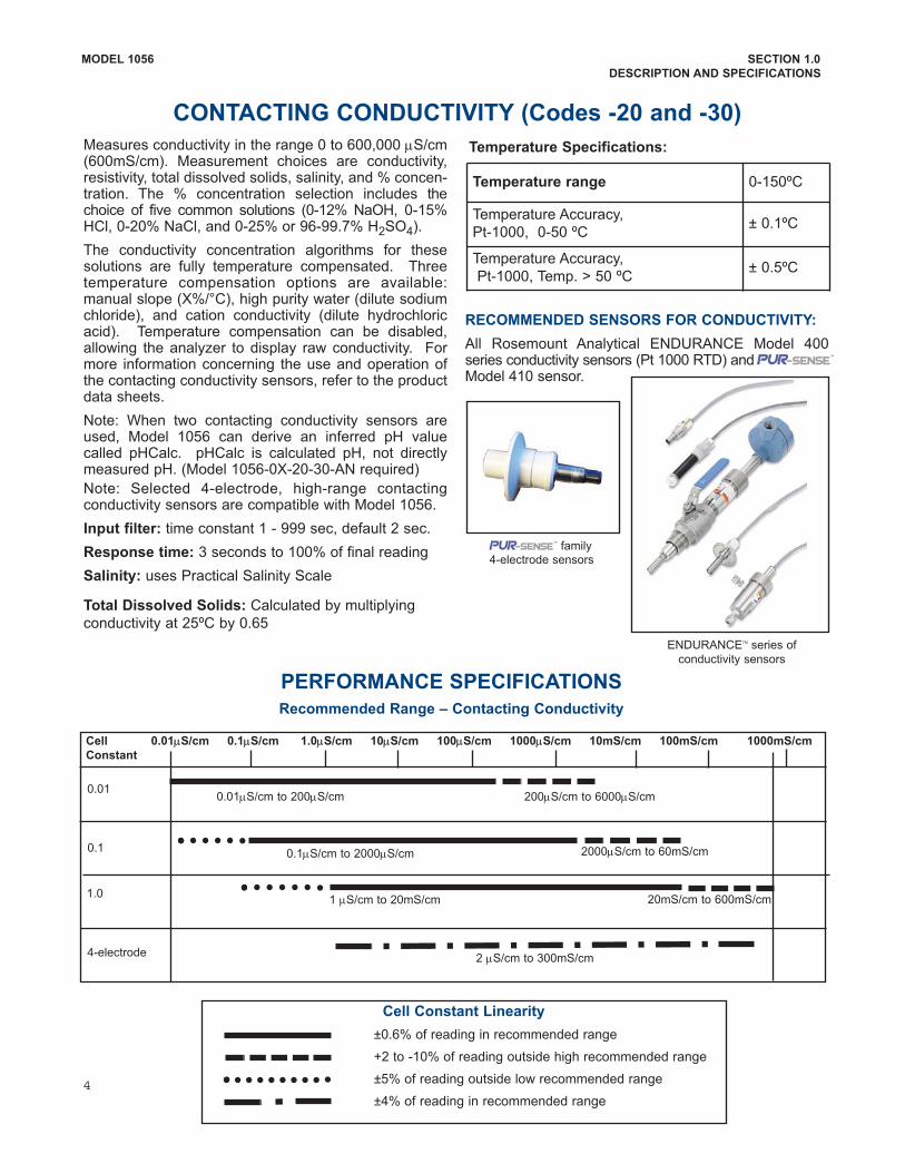
±0.6% of reading in recommended range
+2 to 10% of reading outside high recommended range
±5% of reading outside low recommended range
±4% of reading in recommended range
Measures conductivity in the range 0 to 600,000 μS/cm(600mS/cm). Measurement choices are conductivity,resistivity, total dissolved solids, salinity, and % concentration. The % concentration selection includes thechoice of five common solutions (012% NaOH, 015%HCl, 020% NaCl, and 025% or 9699.7% H2SO4).
The conductivity concentration algorithms for thesesolutions are fully temperature compensated. Threetemperature compensation options are available:manual slope (X%/°C), high purity water (dilute sodiumchloride), and cation conductivity (dilute hydrochloricacid). Temperature compensation can be disabled,allowing the analyzer to display raw conductivity. Formore information concerning the use and operation ofthe contacting conductivity sensors, refer to the productdata sheets.
Note: When two contacting conductivity sensors areused, Model 1056 can derive an inferred pH valuecalled pHCalc. pHCalc is calculated pH, not directlymeasured pH. (Model 10560X2030AN required)
Note: Selected 4electrode, highrange contactingconductivity sensors are compatible with Model 1056.
Input filter: time constant 1 999 sec, default 2 sec.
Response time: 3 seconds to 100% of final reading
Salinity: uses Practical Salinity Scale
Total Dissolved Solids: Calculated by multiplying
conductivity at 25ºC by 0.65
RECOMMENDED SENSORS FOR CONDUCTIVITY:
All Rosemount Analytical ENDURANCE Model 400series conductivity sensors (Pt 1000 RTD) andModel 410 sensor.
CONTACTING CONDUCTIVITY (Codes 20 and 30)
Temperature range 0150ºC
Temperature Accuracy,
Pt1000, 050 ºC± 0.1ºC
Temperature Accuracy,
Pt1000, Temp. > 50 ºC± 0.5ºC
PERFORMANCE SPECIFICATIONS
Recommended Range – Contacting Conductivity
Temperature Specifications:
ENDURANCETM series of
conductivity sensors
family4electrode sensors
Cell Constant Linearity
Cell 0.01μS/cm 0.1μS/cm 1.0μS/cm 10μS/cm 100μS/cm 1000μS/cm 10mS/cm 100mS/cm 1000mS/cm
Constant
0.01
0.1
1.0
4electrode
0.01μS/cm to 200μS/cm
0.1μS/cm to 2000μS/cm
1 μS/cm to 20mS/cm
2 μS/cm to 300mS/cm
200μS/cm to 6000μS/cm
2000μS/cm to 60mS/cm
20mS/cm to 600mS/cm
4
MODEL 1056 SECTION 1.0
DESCRIPTION AND SPECIFICATIONS
Model 1μS/cm 10μS/cm 100μS/cm 1000μS/cm 10mS/cm 100mS/cm 1000mS/cm 2000mS/cm
5μS/cm to 500mS/cm
15μS/cm to 1500mS/cm
500mS/cm to 2000mS/cm
500μS/cm to 2000mS/cm
100μS/cm to 2000mS/cm
1500mS/cm to 2000mS/cm
226
242
222
(1in & 2in)
225 & 228
Measures conductivity in the range of 1 (one) μS/cm to
2,000,000 μS/cm (2 S/cm), Measurement choices are
conductivity, resistivity, total dissolved solids, salinity,
and % concentration. The % concentration selection
includes the choice of five common solutions (012%
NaOH, 015% HCl, 020% NaCl, and 025% or
9699.7% H2SO4). The conductivity concentration
algorithms for these solutions are fully temperature
compensated. For other solutions, a simpletouse
menu allows the customer to enter his own data. The
analyzer accepts as many as five data points and fits
either a linear (two points) or a quadratic function (three
or more points) to the data. Two temperature compensation
options are available: manual slope (X%/°C) and neutral
salt (dilute sodium chloride). Temperature compensation
can be disabled, allowing the analyzer to display raw
conductivity. Reference temperature and linear temper
ature slope may also be adjusted for optimum results.
For more information concerning the use and operation
of the toroidal conductivity sensors, refer to the product
data sheets.
Repeatability: ±0.25% ±5 μS/cm after zero cal
Input filter: time constant 1 999 sec, default 2 sec.
Response time: 3 seconds to 100% of final reading
Salinity: uses Practical Salinity Scale
Total Dissolved Solids: Calculated by multiplying
conductivity at 25ºC by 0.65
Temperature Specifications:
RECOMMENDED SENSORS:
All Rosemount Analytical submersion/immersion and
flowthrough toroidal sensors.
TOROIDAL CONDUCTIVITY (Codes 21 and 31)
Temperature range 25 to 210ºC (13 to 410ºF)
Temperature Accuracy,
Pt100, 25 to 50 ºC± 0.5ºC
Temperature Accuracy,
Pt100,. 50 to 210ºC± 1ºC
PERFORMANCE SPECIFICATIONS
Recommended Range Toroidal Conductivity
Model 226: ±1% of reading ±5μS/cm in recommended range
Models 225 & 228: ±1% of reading ±10μS/cm in recommended range
Models 222,242: ±4% of reading in recommended range
Model 225, 226 & 228: ±5% of reading outside high recommended range
Model 226: ±5μS/cm outside low recommended range
Models 225 & 228: ±15μS/cm outside low recommended range
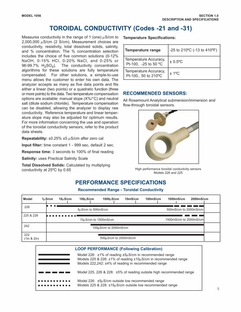
High performance toroidal conductivity sensors
Models 226 and 225
LOOP PERFORMANCE (Following Calibration)
5
6
MODEL 1056 SECTION 1.0
DESCRIPTION AND SPECIFICATIONS
For use with any standard pH or ORP sensor.Measurement choices are pH, ORP, Redox, ammonia,fluoride or custom ISE. The automatic buffer recognitionfeature uses stored buffer values and their temperaturecurves for the most common buffer standards availableworldwide. The analyzer will recognize the value of thebuffer being measured and perform a self stabilizationcheck on the sensor before completing the calibration.Manual or automatic temperature compensation ismenu selectable. Change in pH due to process temperature can be compensated using a programmable temperature coefficient. For more information concerningthe use and operation of the pH or ORP sensors, referto the product data sheets.
Model 1056 can also derive an inferred pH value calledpHCalc (calculated pH). pHCalc can be derived anddisplayed when two contacting conductivity sensors areused. (Model 10560X2030AN)
PERFORMANCE SPECIFICATIONS ANALYZER (pH INPUT)
Measurement Range [pH]: 0 to 14 pH
Accuracy: ±0.01 pH
Diagnostics: glass impedance, reference impedance
Temperature coefficient: ±0.002pH/ ºC
Solution temperature correction: pure water, dilutebase and custom.
Buffer recognition: NIST, DIN 19266, JIS 8802, BSI,DIN19267, Ingold, and Merck.
Input filter: time constant 1 999 seconds, default 4seconds.
Response time: 5 seconds to 100%
Temperature Specifications:
PERFORMANCE SPECIFICATIONS ANALYZER (ORP INPUT)
Measurement Range [ORP]: 1500 to +1500 mV
Accuracy: ± 1 mV
Temperature coefficient: ±0.12mV / ºC
Input filter: time constant 1 999 seconds, default 4seconds.
Response time: 5 seconds to 100% of final reading
RECOMMENDED SENSORS FOR pH:
All standard pH sensors.
RECOMMENDED SENSORS FOR ORP:
All standard ORP sensors.
Temperature range 0150ºC
Temperature Accuracy, Pt100, 050 ºC ± 0.5ºC
Temperature Accuracy, Temp. > 50 ºC ± 1ºC
pH/ORP/ISE (Codes 22 and 32)
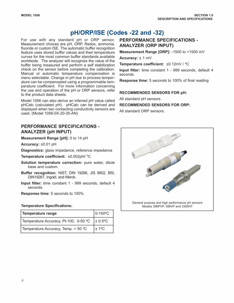
General purpose and high performance pH sensors
Models 396PVP, 399VP and 3300HT
7
MODEL 1056 SECTION 1.0
DESCRIPTION AND SPECIFICATIONS
FLOW (Code 23 and 33)
420mA Current Input (Codes 23 and 33)
For use with most pulse signal flow sensors, the 1056userselectable units of measurement include flow ratesin GPM (Gallons per minute), GPH (Gallon per hour), cuft/min (cubic feet per min), cu ft/hour (cubic feet perhour), LPM (liters per minute), LPH (liters per hour), orm3/hr (cubic meters per hour), and velocity in ft/sec orm/sec. When configured to measure flow, the unit alsoacts as a totalizer in the chosen unit (gallons, liters, orcubic meters).
Dual flow instruments can be configured as a % recovery,flow difference, flow ratio, or total (combined) flow.
PERFORMANCE SPECIFICATIONS
Frequency Range: 3 to 1000 Hz
Flow Rate: 0 99,999 GPM, LPM, m3/hr, GPH, LPH,cu ft/min, cu ft/hr.
Totalized Flow: 0 – 9,999,999,999,999 Gallons or m3,0 – 999, 999,999,999 cu ft.
Accuracy: 0.5%
Input filter: time constant 0999 sec., default 5 sec.
RECOMMENDED SENSORS*
+GF+ Signet 515 RotorX Flow sensor
* Input voltage not to exceed ±36V
For use with any transmitter or external device thattransmits 420mA or 020mA current outputs. Typicaluses are for temperature compensation of live measurements (except ORP, turbidity and flow) and forcontinuous atmospheric pressure input for determination of partial pressure, needed for compensation of livedissolved oxygen measurements. External input ofatmospheric pressure for DO measurement allowscontinuous partial pressure compensation while theModel 1056 enclosure is completely sealed. (Thepressure transducer component on the DO board canonly be used for calibration when the case is open toatmosphere.)
Externally sourced current input is also useful forcalibration of new or existing sensors that requiretemperature measurement or atmospheric pressureinputs (DO only).
For externally sourced temp or pressure compensation,the user must program the 1056 to input the 420mAcurrent signal from the external device.
In addition to live continuous compensation of livemeasurements, the current input board can also beused simply to display the measured temperature. orthe calculated partial pressure from the external device.
This feature leverages the large display variables on theModel 1056 as a convenience for technicians.Temperature can be displayed in degrees C or degreesF. Partial pressure can be displayed in inches Hg, mmHg, atm (atmospheres), kPa (kiloPascals), bar or mbar.
The current input board can be used with devices thatdo not actively power their 420mA output signals. TheModel 1056 actively powers to the + and – lines of thecurrent input board to enable current input from a420mA output device.
Note: this Model 1056 signal input board (23, 33model option code) also includes flow measurementfunctionality. The signal board, however, must beconfigured to measure either mA current input or flow.
PERFORMANCE SPECIFICATIONS
Measurement Range *[mA]: 020 or 420
Accuracy: ±0.03mA
Input filter: time constant 0999 sec., default 5 sec.
*Current input not to exceed 22mA
MODEL 1056 SECTION 1.0
DESCRIPTION AND SPECIFICATIONS
Free and Total ChlorineThe 1056 is compatible with the 499ACL01 free chlorinesensor and the 499ACL02 total chlorine sensor. The499ACL02 sensor must be used with the TCL totalchlorine sample conditioning system. The 1056 fullycompensates free and total chlorine readings forchanges in membrane permeability caused by temperature changes. For free chlorine measurements, bothautomatic and manual pH correction are available. Forautomatic pH correction select code 32 and an appropriate pH sensor. For more information concerning the useand operation of the amperometric chlorine sensors andthe TCL measurement system, refer to the product datasheets.
PERFORMANCE SPECIFICATIONSResolution: 0.001 ppm or 0.01 ppm – selectable
Input Range: 0nA – 100μA
Automatic pH correction (requires Code 32): 6.0 to10.0 pH
Temperature compensation: Automatic (via RTD) ormanual (050°C).
Input filter: time constant 1 999 sec, default 5 sec.
Response time: 6 seconds to 100% of final reading
RECOMMENDED SENSORS*
Chlorine: Model 499ACL01 Free Chlorine or Model499ACL02 Total Residual Chlorine
pH: The following pH sensors are recommended for
automatic pH correction of free chlorine readings:
Models: 3990962, 39914, and 399VP09
MonochloramineThe Model 1056 is compatible with the Model 499A CL03Monochloramine sensor. The Model 1056 fullycompensates readings for changes in membranepermeability caused by temperature changes. Becausemonochloramine measurement is not affected by pH ofthe process, no pH sensor or correction is required. Formore information concerning the use and operation of theamperometric chlorine sensors, refer to the product datasheets.
PERFORMANCE SPECIFICATIONSResolution: 0.001 ppm or 0.01 ppm – selectable
Input Range: 0nA – 100μA
Temperature compensation: Automatic (via RTD) ormanual (050°C).
Input filter: time constant 1 999 sec, default 5 sec.
Response time: 6 seconds to 100% of final reading
RECOMMENDED SENSORSRosemount Analytical Model 499ACL03 Monochloraminesensor
pHIndependent Free ChlorineThe 1056 is compatible with the Model 498CL01 pHindependent free chlorine sensor. The Model 498CL01sensor is intended for the continuous determination offree chlorine (hypochlorous acid plus hypochlorite ion)in water. The primary application is measuring chlorinein drinking water. The sensor requires no acid pretreatment, nor is an auxiliary pH sensor required for pHcorrection. The Model 1056 fully compensates freechlorine readings for changes in membranepermeability caused by temperature. For more informationconcerning the use and operation of the amperometricchlorine sensors, refer to the product data sheets.
PERFORMANCE SPECIFICATIONSResolution: 0.001 ppm or 0.01 ppm – selectable
Input Range: 0nA – 100μA
Automatic pH correction: 6.5 to 10.0 pH
Temperature compensation: Automatic (via RTD) ormanual (050°C).
Input filter: time constant 1 999 sec, default 5 sec.
Response time: 6 seconds to 100% of final reading
RECOMMENDED SENSORSRosemount Analytical Model 498CL01 pH independent
free chlorine sensor
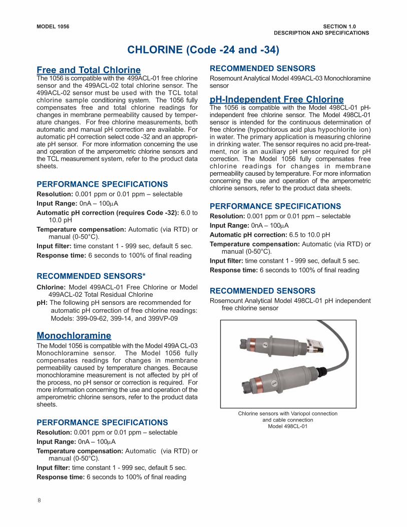
CHLORINE (Code 24 and 34)
Chlorine sensors with Variopol connection
and cable connection
Model 498CL01
8
MODEL 1056 SECTION 1.0
DESCRIPTION AND SPECIFICATIONS
DISSOLVED OXYGEN(Codes 25 and 35)
The 1056 is compatible with the 499ADO, 499ATrDO,Hx438, and Gx438 dissolved oxygen sensors and the4000 percent oxygen gas sensor. The 1056 displaysdissolved oxygen in ppm, mg/L, ppb, μg/L, % saturation, % O2 in gas, ppm O2 in gas. The analyzer fullycompensates oxygen readings for changes in membrane permeability caused by temperature changes.An atmospheric pressure sensor is included on all dissolved oxygen signal boards to allow automatic atmospheric pressure determination at the time of calibration.If removing the sensor from the process liquid is impractical, the analyzer can be calibrated against a standardinstrument. Calibration can be corrected for processsalinity. For more information on the use of amperometric oxygen sensors, refer to the product datasheets.
PERFORMANCE SPECIFICATIONSResolution: 0.01 ppm; 0.1 ppb for 499A TrDO sensor
(when O2 <1.00 ppm); 0.1%
Input Range: 0nA – 100μA
Temperature Compensation: Automatic (via RTD) ormanual (050°C).
Input filter: time constant 1 999 sec, default 5 sec.
Response time: 6 seconds to 100% of final reading
RECOMMENDED SENSORSRosemount Analytical amperometric membrane and
steamsterilizable sensors listed above
DISSOLVED OZONE (Code 26 and 36)
The 1056 is compatible with the Model 499AOZ sensor. The 1056 fully compensates ozone readings forchanges in membrane permeability caused by temperature changes. For more information concerning theuse and operation of the amperometric ozone sensors,refer to the product data sheets.
PERFORMANCE SPECIFICATIONSResolution: 0.001 ppm or 0.01 ppm – selectable
Input Range: 0nA – 100μA
Temperature Compensation: Automatic (via RTD) ormanual (035°C)
Input filter: time constant 1 999 sec, default 5 sec.
Response time: 6 seconds to 100% of final reading
RECOMMENDED SENSORRosemount Analytical Model 499A OZ ozone sensor
Dissolved Oxygen sensor with Variopol connection
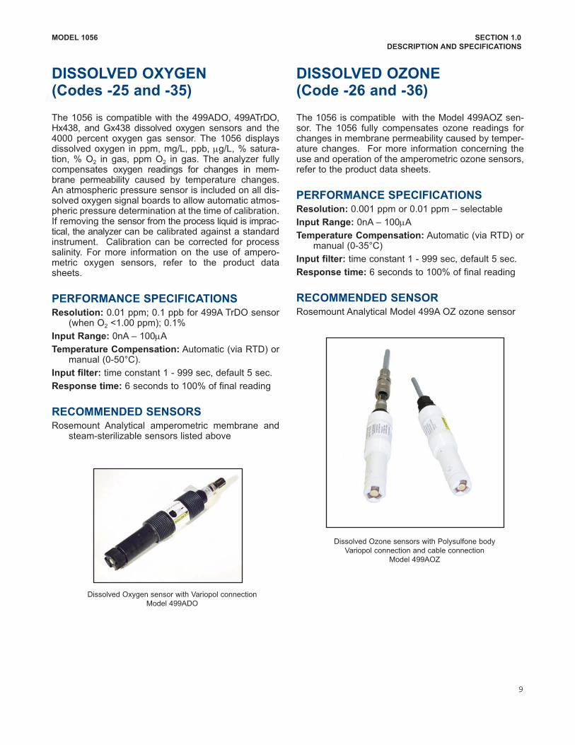
Model 499ADO
Dissolved Ozone sensors with Polysulfone body
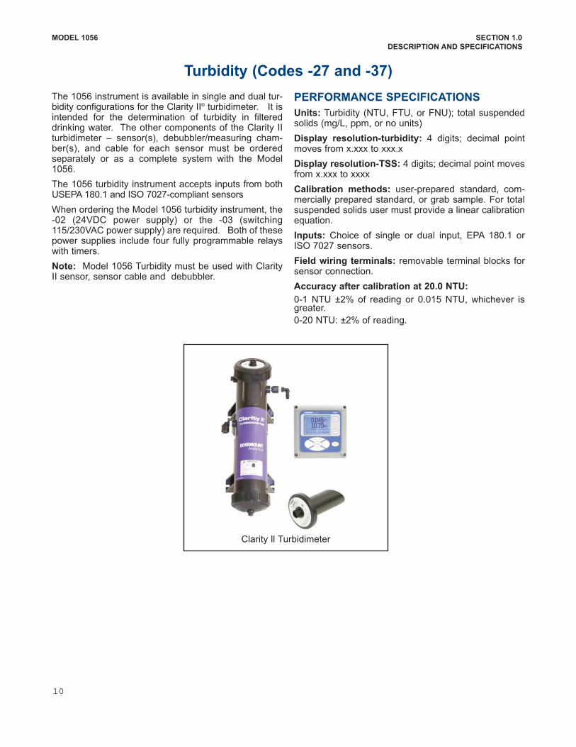
Variopol connection and cable connection
Model 499AOZ
9
Turbidity (Codes 27 and 37)
The 1056 instrument is available in single and dual turbidity configurations for the Clarity II® turbidimeter. It isintended for the determination of turbidity in filtereddrinking water. The other components of the Clarity IIturbidimeter – sensor(s), debubbler/measuring chamber(s), and cable for each sensor must be orderedseparately or as a complete system with the Model1056.
The 1056 turbidity instrument accepts inputs from bothUSEPA 180.1 and ISO 7027compliant sensors
When ordering the Model 1056 turbidity instrument, the02 (24VDC power supply) or the 03 (switching115/230VAC power supply) are required. Both of thesepower supplies include four fully programmable relayswith timers.
Note: Model 1056 Turbidity must be used with ClarityII sensor, sensor cable and debubbler.
PERFORMANCE SPECIFICATIONS
Units: Turbidity (NTU, FTU, or FNU); total suspendedsolids (mg/L, ppm, or no units)
Display resolutionturbidity: 4 digits; decimal pointmoves from x.xxx to xxx.x
Display resolutionTSS: 4 digits; decimal point movesfrom x.xxx to xxxx
Calibration methods: userprepared standard, commercially prepared standard, or grab sample. For totalsuspended solids user must provide a linear calibrationequation.
Inputs: Choice of single or dual input, EPA 180.1 orISO 7027 sensors.
Field wiring terminals: removable terminal blocks forsensor connection.
Accuracy after calibration at 20.0 NTU:
01 NTU ±2% of reading or 0.015 NTU, whichever isgreater.
020 NTU: ±2% of reading.
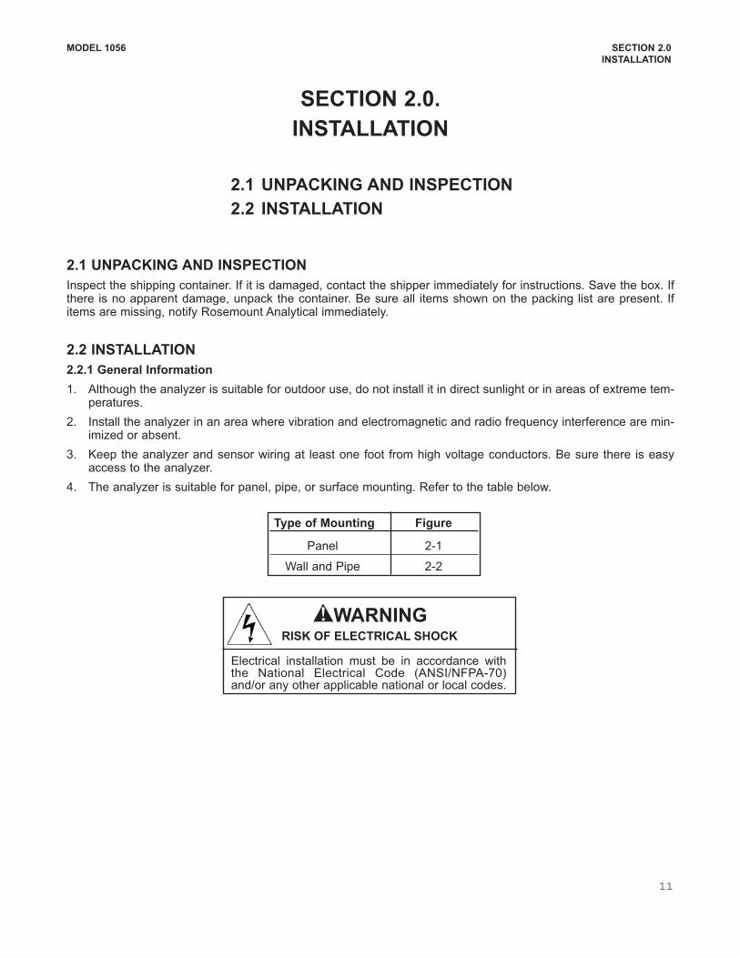
Clarity ll Turbidimeter
MODEL 1056 SECTION 1.0
DESCRIPTION AND SPECIFICATIONS
10
SECTION 2.0.
INSTALLATION
MODEL 1056 SECTION 2.0
INSTALLATION
2.1 UNPACKING AND INSPECTION
2.2 INSTALLATION
Type of Mounting Figure
Panel 21
Wall and Pipe 22
2.1 UNPACKING AND INSPECTION
Inspect the shipping container. If it is damaged, contact the shipper immediately for instructions. Save the box. Ifthere is no apparent damage, unpack the container. Be sure all items shown on the packing list are present. Ifitems are missing, notify Rosemount Analytical immediately.
2.2 INSTALLATION
2.2.1 General Information
1. Although the analyzer is suitable for outdoor use, do not install it in direct sunlight or in areas of extreme temperatures.
2. Install the analyzer in an area where vibration and electromagnetic and radio frequency interference are minimized or absent.
3. Keep the analyzer and sensor wiring at least one foot from high voltage conductors. Be sure there is easyaccess to the analyzer.
4. The analyzer is suitable for panel, pipe, or surface mounting. Refer to the table below.
11
Electrical installation must be in accordance withthe National Electrical Code (ANSI/NFPA70)and/or any other applicable national or local codes.
WARNINGRISK OF ELECTRICAL SHOCK
Bottom View
Front View
Side View
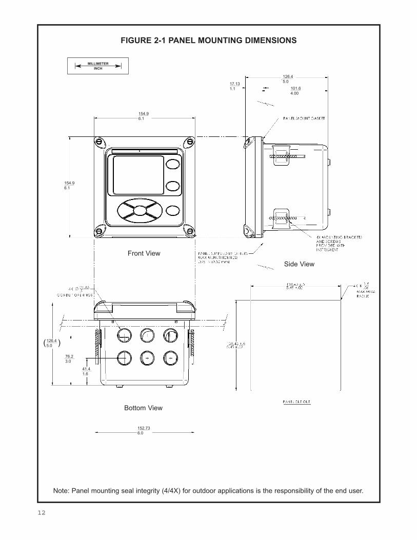
FIGURE 21 PANEL MOUNTING DIMENSIONS
Note: Panel mounting seal integrity (4/4X) for outdoor applications is the responsibility of the end user.
MILLIMETER
INCH
154.9
6.1
154.9
6.1
126.4
5.0
101.6
4.00
17.13
1.1
126.4
5.0 )(
76.2
3.0
41.4
1.6
152.73
6.0
12

FIGURE 22 PIPE AND WALL MOUNTING DIMENSIONS
(Mounting bracket PN:2382000)
The front panel is hinged at the bottom. The panel swings down for easy access to the wiring locations.
Bottom View
Front View
Side View
Side View
Wall / Surface Mount
Pipe Mount
MILLIMETER
INCH
154.9
6.1
102
4.0
187
7.4154.9
6.1
232
9.1
33.5
1.3
130
5.1
165
6.5
232
9.1
130
5.1
33.5
1.3
165
6.5
108.9
4.3
45.21
1.8
80.01
3.2
71.37
2.8
13
MODEL 1056 SECTION 2.0
INSTALLATION
FIG
UR
E 2
3 C
SA
NonI
ncendiv
e C
lass I
, D
ivis
ion 2
Cert
ifie
d p
roduct
for
sele
cte
d c
onfigura
tions (
for
appro
ved m
odels
, see F
ig.
24
)
14
MODEL 1056 SECTION 2.0
INSTALLATION
FIG
UR
E 2
4 C
SA
NonI
ncendiv
e C
lass I
, D
ivis
ion 2
Cert
ifie
d p
roduct
for
sele
cte
d c
onfigura
tions
15
16
FIG
UR
E 2
5 F
M N
onI
ncendiv
e C
lass I
, D
ivis
ion 2
Cert
ifie
d p
roduct
for
sele
cte
d c
onfigura
tions (
for
appro
ved m
odels
, see F
ig.
26
)
MODEL 1056 SECTION 2.0
INSTALLATION
17
FIG
UR
E 2
6 F
M N
onI
ncendiv
e C
lass I
, D
ivis
ion 2
Cert
ifie
d p
roduct
for
sele
cte
d c
onfigura
tions
MODEL 1056 SECTION 2.0
INSTALLATION

This page left blank intentionally
MODEL 1056 SECTION 2.0
INSTALLATION
18
SECTION 3.0.
WIRING3.1 GENERAL3.2 PREPARING CONDUIT OPENINGS3.3 PREPARING SENSOR CABLE3.4 POWER, OUTPUT, AND SENSOR
CONNECTIONS
MODEL 1056 SECTION 3.0
WIRING
3.1 GENERAL The 1056 is easy to wire. It includes removable connectors and slideout signal input boards. The front panel is
hinged at the bottom. The panel swings down for easy access to the wiring locations.
3.1.1. Removable connectors and signal input boards
Model 1056 uses removable signal input boards and communication boards for ease of wiring and instal
lation. Each of the signal input boards can be partially or completely removed from the enclosure for wiring.
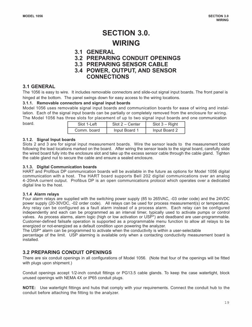
The Model 1056 has three slots for placement of up to two signal input boards and one communication
board.
3.1.2. Signal Input boards Slots 2 and 3 are for signal input measurement boards. Wire the sensor leads to the measurement boardfollowing the lead locations marked on the board. After wiring the sensor leads to the signal board, carefully slidethe wired board fully into the enclosure slot and take up the excess sensor cable through the cable gland. Tightenthe cable gland nut to secure the cable and ensure a sealed enclosure.
3.1.3. Digital Communication boardsHART and Profibus DP communication boards will be available in the future as options for Model 1056 digitalcommunication with a host. The HART board supports Bell 202 digital communications over an analog420mA current output. Profibus DP is an open communications protocol which operates over a dedicateddigital line to the host.
3.1.4 Alarm relays Four alarm relays are supplied with the switching power supply (85 to 265VAC, 03 order code) and the 24VDCpower supply (2030VDC, 02 order code). All relays can be used for process measurement(s) or temperature.Any relay can be configured as a fault alarm instead of a process alarm. Each relay can be configuredindependently and each can be programmed as an interval timer, typically used to activate pumps or controlvalves. As process alarms, alarm logic (high or low activation or USP*) and deadband are userprogrammable.Customerdefined failsafe operation is supported as a programmable menu function to allow all relays to beenergized or notenergized as a default condition upon powering the analyzer.The USP* alarm can be programmed to activate when the conductivity is within a userselectablepercentage of the limit. USP alarming is available only when a contacting conductivity measurement board isinstalled.
3.2 PREPARING CONDUIT OPENINGSThere are six conduit openings in all configurations of Model 1056. (Note that four of the openings will be fitted
with plugs upon shipment.)
Conduit openings accept 1/2inch conduit fittings or PG13.5 cable glands. To keep the case watertight, block
unused openings with NEMA 4X or IP65 conduit plugs.
NOTE: Use watertight fittings and hubs that comply with your requirements. Connect the conduit hub to the
conduit before attaching the fitting to the analyzer.
Slot 1Left Slot 2 – Center Slot 3 – Right
Comm. board Input Board 1 Input Board 2
19
MODEL 1056 SECTION 3.0
WIRING
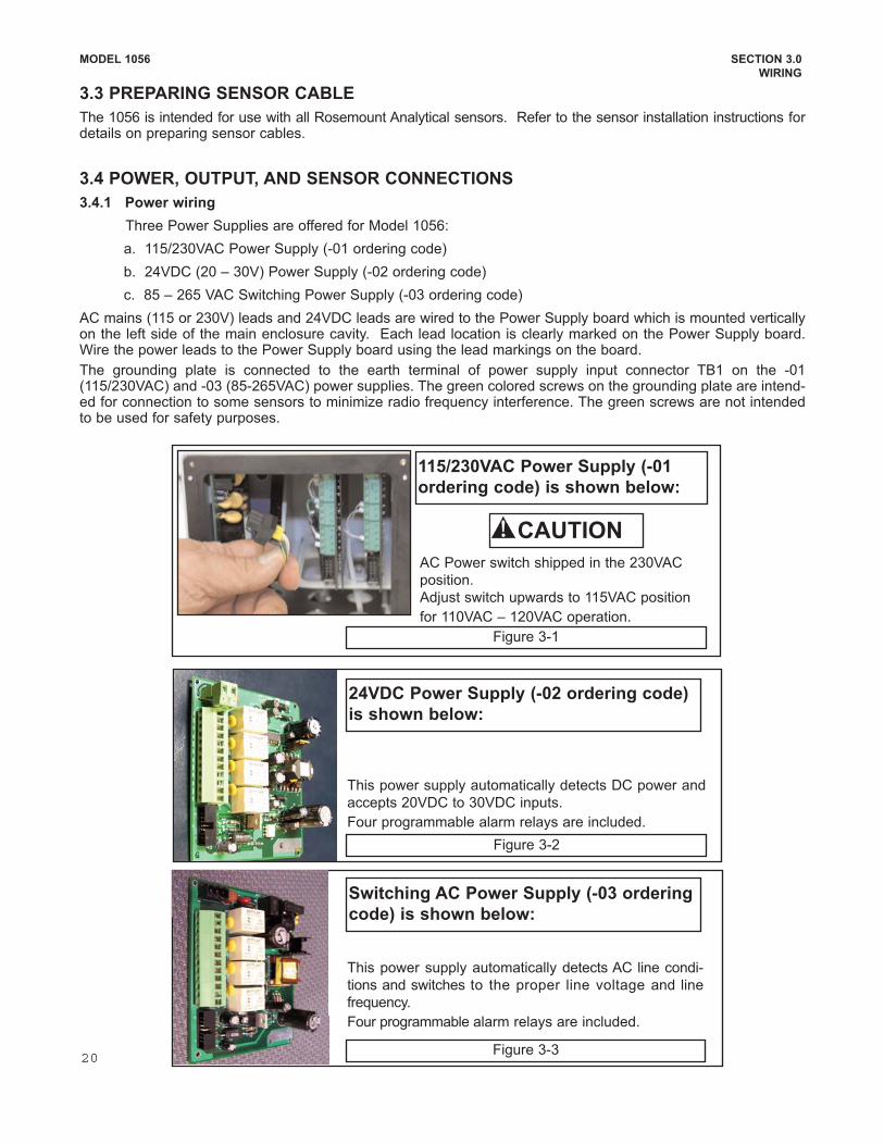
AC Power switch shipped in the 230VAC
position.
Adjust switch upwards to 115VAC position
for 110VAC – 120VAC operation.
This power supply automatically detects DC power and
accepts 20VDC to 30VDC inputs.
Four programmable alarm relays are included.
Figure 31
Figure 32
This power supply automatically detects AC line condi
tions and switches to the proper line voltage and line
frequency.
Four programmable alarm relays are included.
Figure 33
Switching AC Power Supply (03 ordering
code) is shown below:
24VDC Power Supply (02 ordering code)
is shown below:
115/230VAC Power Supply (01
ordering code) is shown below:
20
3.3 PREPARING SENSOR CABLE
The 1056 is intended for use with all Rosemount Analytical sensors. Refer to the sensor installation instructions fordetails on preparing sensor cables.
3.4 POWER, OUTPUT, AND SENSOR CONNECTIONS
3.4.1 Power wiring
Three Power Supplies are offered for Model 1056:
a. 115/230VAC Power Supply (01 ordering code)
b. 24VDC (20 – 30V) Power Supply (02 ordering code)
c. 85 – 265 VAC Switching Power Supply (03 ordering code)
AC mains (115 or 230V) leads and 24VDC leads are wired to the Power Supply board which is mounted verticallyon the left side of the main enclosure cavity. Each lead location is clearly marked on the Power Supply board.Wire the power leads to the Power Supply board using the lead markings on the board.
The grounding plate is connected to the earth terminal of power supply input connector TB1 on the 01(115/230VAC) and 03 (85265VAC) power supplies. The green colored screws on the grounding plate are intended for connection to some sensors to minimize radio frequency interference. The green screws are not intendedto be used for safety purposes.
CAUTION
MODEL 1056 SECTION 3.0
WIRING
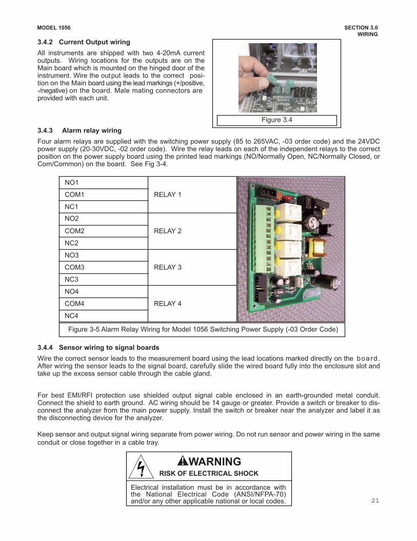
Figure 35 Alarm Relay Wiring for Model 1056 Switching Power Supply (03 Order Code)
NO1
RELAY 1COM1
NC1
NO2
RELAY 2COM2
NC2
NO3
RELAY 3COM3
NC3
NO4
RELAY 4COM4
NC4
3.4.4 Sensor wiring to signal boards
Wire the correct sensor leads to the measurement board using the lead locations marked directly on the board.After wiring the sensor leads to the signal board, carefully slide the wired board fully into the enclosure slot andtake up the excess sensor cable through the cable gland.
For best EMI/RFI protection use shielded output signal cable enclosed in an earthgrounded metal conduit.Connect the shield to earth ground. AC wiring should be 14 gauge or greater. Provide a switch or breaker to disconnect the analyzer from the main power supply. Install the switch or breaker near the analyzer and label it asthe disconnecting device for the analyzer.
Keep sensor and output signal wiring separate from power wiring. Do not run sensor and power wiring in the same
conduit or close together in a cable tray.
3.4.3 Alarm relay wiring
Four alarm relays are supplied with the switching power supply (85 to 265VAC, 03 order code) and the 24VDCpower supply (2030VDC, 02 order code). Wire the relay leads on each of the independent relays to the correctposition on the power supply board using the printed lead markings (NO/Normally Open, NC/Normally Closed, orCom/Common) on the board. See Fig 34.
3.4.2 Current Output wiring
All instruments are shipped with two 420mA currentoutputs. Wiring locations for the outputs are on theMain board which is mounted on the hinged door of theinstrument. Wire the output leads to the correct position on the Main board using the lead markings (+/positive,/negative) on the board. Male mating connectors areprovided with each unit.
Figure 3.4
21
Electrical installation must be in accordance withthe National Electrical Code (ANSI/NFPA70)and/or any other applicable national or local codes.
WARNINGRISK OF ELECTRICAL SHOCK
MODEL 1056 SECTION 3.0
WIRING
Sec. 3.4 Signal board wiring
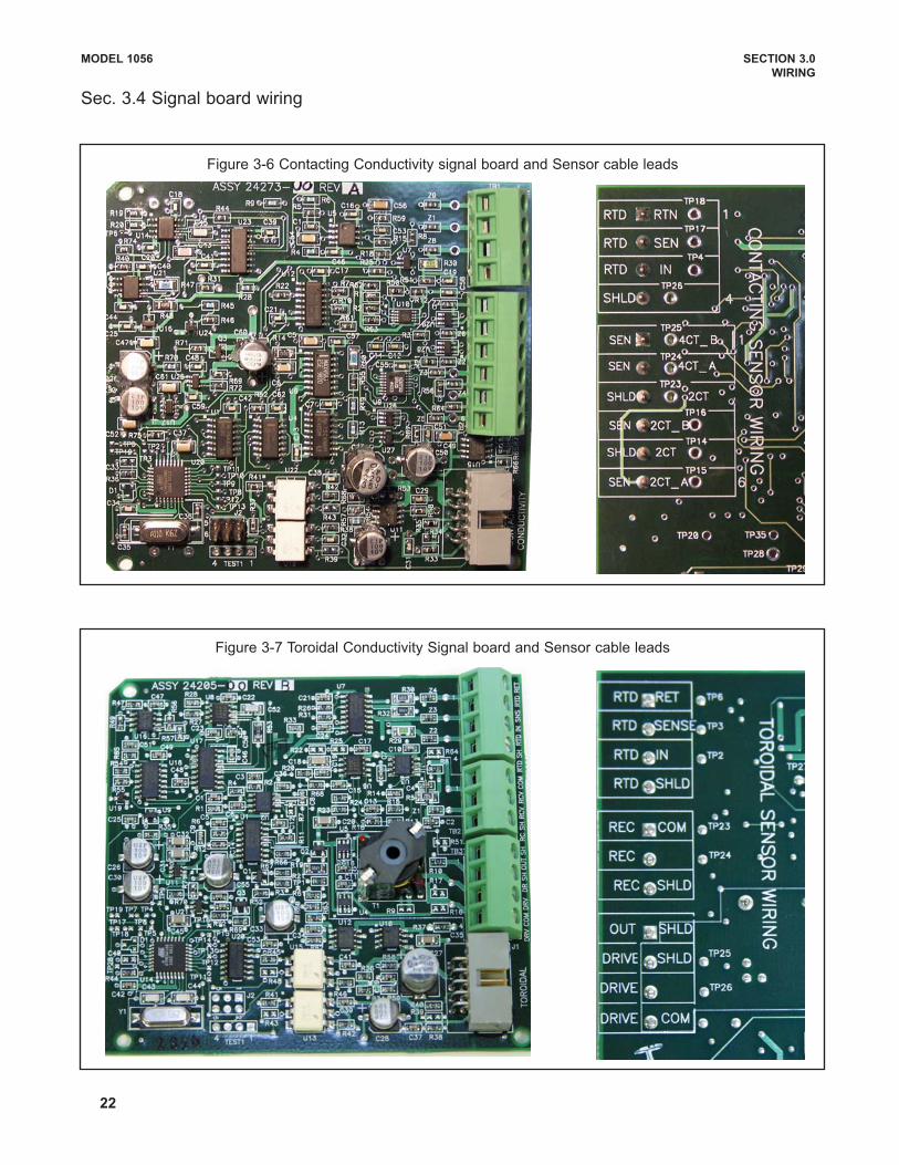
Figure 36 Contacting Conductivity signal board and Sensor cable leads
Figure 37 Toroidal Conductivity Signal board and Sensor cable leads
22
MODEL 1056 SECTION 3.0
WIRING
Figure 38 pH/ORP/ISE signal board and Sensor cable leads
Figure 39 Amperometric signal (Chlorine, Oxygen, Ozone) board and Sensor cable leads
23
MODEL 1056 SECTION 3.0
WIRING
Figure 310 Turbidity signal board with plugin Sensor connection
Figure 311 Flow/Current Input signal board and Sensor cable leads
24
MODEL 1056 SECTION 3.0
WIRING
FIGURE 312 Power Wiring for the 1056 115/230VAC Power Supply (01 Order Code)
FIGURE 313 Power Wiring for the 1056 85265 VAC Power Supply (03 ordering code)
25
MODEL 1056 SECTION 3.0
WIRING
FIGURE 314 Output Wiring for Model 1056 Main PCB
FIGURE 315 Power Wiring for Model 1056 24VDC Power Supply (02 ordering code)
26
To M
ain
PC
B
MODEL 1056 SECTION 4.0
DISPLAY AND OPERATION
SECTION 4.0
DISPLAY AND OPERATION
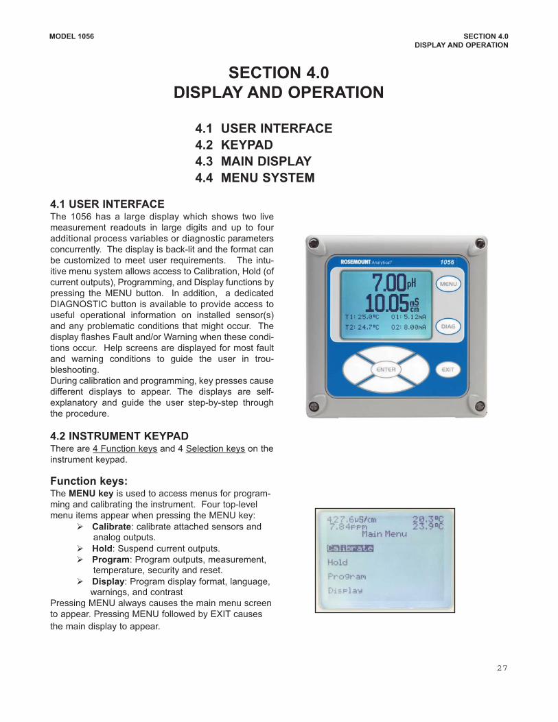
4.1 USER INTERFACEThe 1056 has a large display which shows two live
measurement readouts in large digits and up to four
additional process variables or diagnostic parameters
concurrently. The display is backlit and the format can
be customized to meet user requirements. The intu
itive menu system allows access to Calibration, Hold (of
current outputs), Programming, and Display functions by
pressing the MENU button. In addition, a dedicated
DIAGNOSTIC button is available to provide access to
useful operational information on installed sensor(s)
and any problematic conditions that might occur. The
display flashes Fault and/or Warning when these condi
tions occur. Help screens are displayed for most fault
and warning conditions to guide the user in trou
bleshooting.
During calibration and programming, key presses cause
different displays to appear. The displays are self
explanatory and guide the user stepbystep through
the procedure.
4.2 INSTRUMENT KEYPADThere are 4 Function keys and 4 Selection keys on the
instrument keypad.
Function keys: The MENU key is used to access menus for program
ming and calibrating the instrument. Four toplevel
menu items appear when pressing the MENU key:
Calibrate: calibrate attached sensors and analog outputs.
Hold: Suspend current outputs.
Program: Program outputs, measurement, temperature, security and reset.
Display: Program display format, language, warnings, and contrast
Pressing MENU always causes the main menu screen
to appear. Pressing MENU followed by EXIT causes
the main display to appear.
4.1 USER INTERFACE
4.2 KEYPAD
4.3 MAIN DISPLAY
4.4 MENU SYSTEM
27
MODEL 1056 SECTION 4.0
DISPLAY AND OPERATION
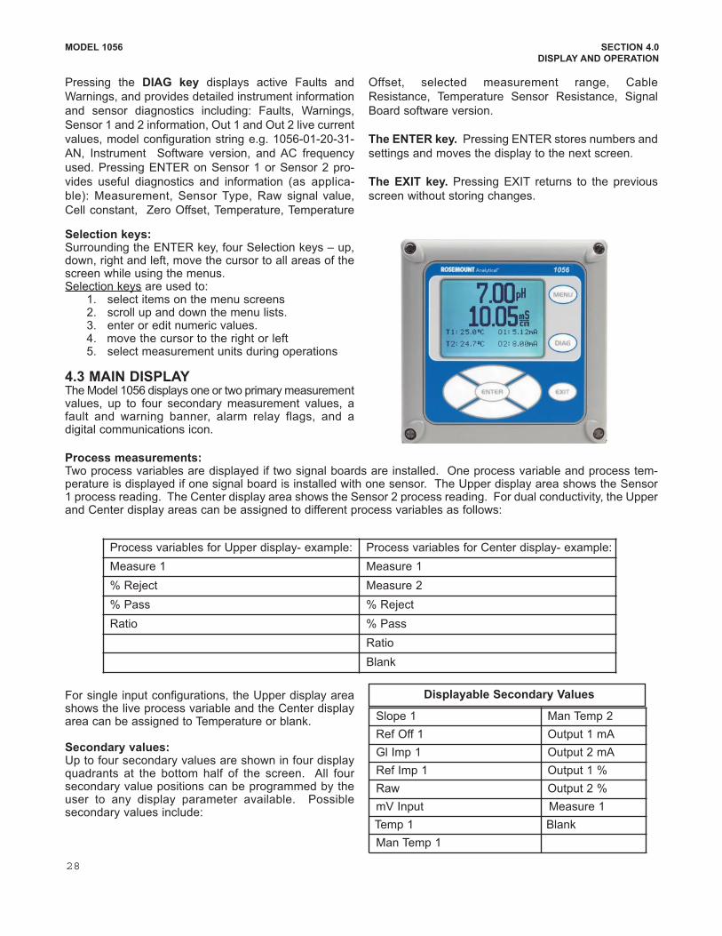
Selection keys: Surrounding the ENTER key, four Selection keys – up,down, right and left, move the cursor to all areas of thescreen while using the menus. Selection keys are used to:
1. select items on the menu screens 2. scroll up and down the menu lists. 3. enter or edit numeric values. 4. move the cursor to the right or left 5. select measurement units during operations
4.3 MAIN DISPLAYThe Model 1056 displays one or two primary measurementvalues, up to four secondary measurement values, afault and warning banner, alarm relay flags, and adigital communications icon.
Process measurements: Two process variables are displayed if two signal boards are installed. One process variable and process temperature is displayed if one signal board is installed with one sensor. The Upper display area shows the Sensor1 process reading. The Center display area shows the Sensor 2 process reading. For dual conductivity, the Upperand Center display areas can be assigned to different process variables as follows:
Process variables for Upper display example: Process variables for Center display example:
Measure 1 Measure 1
% Reject Measure 2
% Pass % Reject
Ratio % Pass
Ratio
Blank
For single input configurations, the Upper display areashows the live process variable and the Center displayarea can be assigned to Temperature or blank.
Secondary values: Up to four secondary values are shown in four displayquadrants at the bottom half of the screen. All foursecondary value positions can be programmed by theuser to any display parameter available. Possiblesecondary values include:
Slope 1 Man Temp 2
Ref Off 1 Output 1 mA
Gl Imp 1 Output 2 mA
Ref Imp 1 Output 1 %
Raw Output 2 %
mV Input Measure 1
Temp 1 Blank
Man Temp 1
Pressing the DIAG key displays active Faults and
Warnings, and provides detailed instrument information
and sensor diagnostics including: Faults, Warnings,
Sensor 1 and 2 information, Out 1 and Out 2 live current
values, model configuration string e.g. 1056012031
AN, Instrument Software version, and AC frequency
used. Pressing ENTER on Sensor 1 or Sensor 2 pro
vides useful diagnostics and information (as applica
ble): Measurement, Sensor Type, Raw signal value,
Cell constant, Zero Offset, Temperature, Temperature
Offset, selected measurement range, Cable
Resistance, Temperature Sensor Resistance, Signal
Board software version.
The ENTER key. Pressing ENTER stores numbers and
settings and moves the display to the next screen.
The EXIT key. Pressing EXIT returns to the previous
screen without storing changes.
Displayable Secondary Values
28
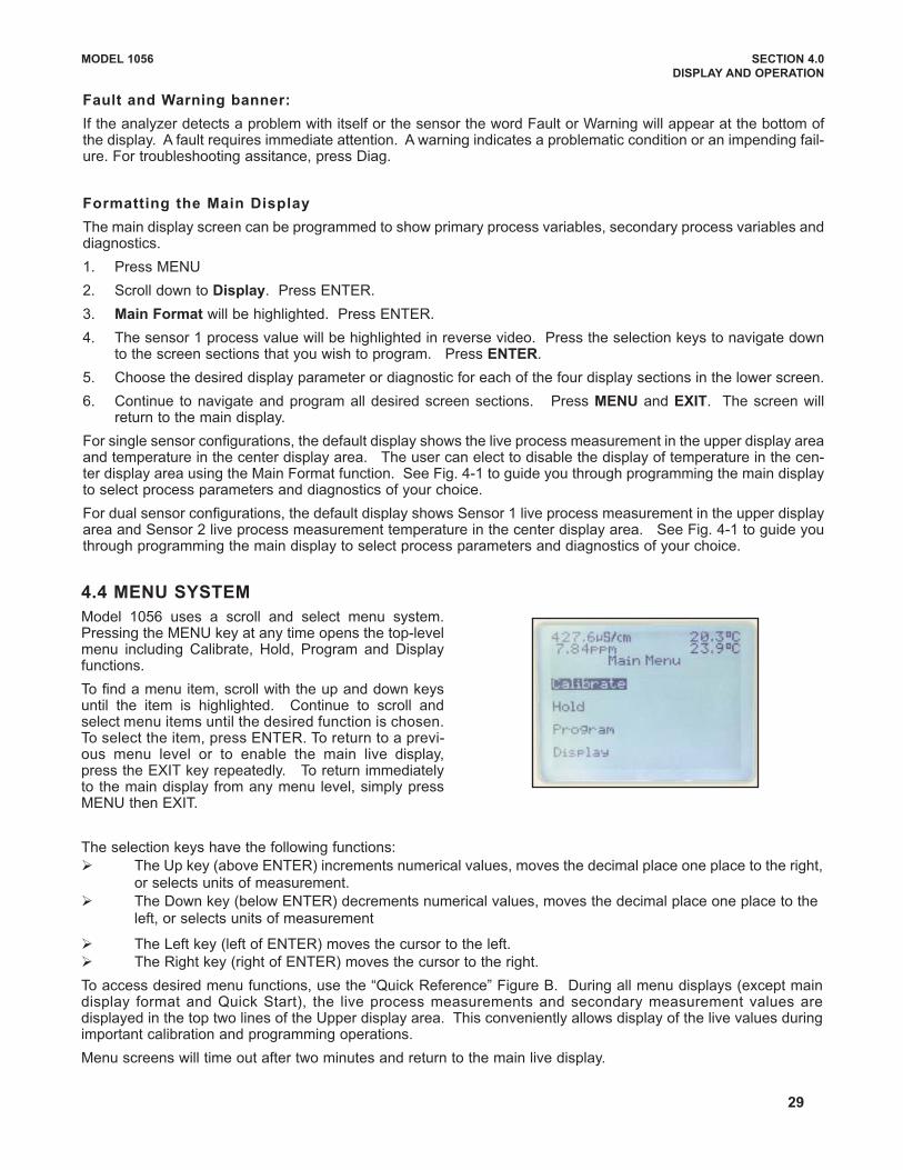
4.4 MENU SYSTEM
Model 1056 uses a scroll and select menu system.Pressing the MENU key at any time opens the toplevelmenu including Calibrate, Hold, Program and Displayfunctions.
To find a menu item, scroll with the up and down keysuntil the item is highlighted. Continue to scroll andselect menu items until the desired function is chosen.To select the item, press ENTER. To return to a previous menu level or to enable the main live display,press the EXIT key repeatedly. To return immediatelyto the main display from any menu level, simply pressMENU then EXIT.
MODEL 1056 SECTION 4.0
DISPLAY AND OPERATION
29
Fault and Warning banner:
If the analyzer detects a problem with itself or the sensor the word Fault or Warning will appear at the bottom ofthe display. A fault requires immediate attention. A warning indicates a problematic condition or an impending failure. For troubleshooting assitance, press Diag.
Formatting the Main Display
The main display screen can be programmed to show primary process variables, secondary process variables anddiagnostics.
1. Press MENU
2. Scroll down to Display. Press ENTER.
3. Main Format will be highlighted. Press ENTER.
4. The sensor 1 process value will be highlighted in reverse video. Press the selection keys to navigate downto the screen sections that you wish to program. Press ENTER.
5. Choose the desired display parameter or diagnostic for each of the four display sections in the lower screen.
6. Continue to navigate and program all desired screen sections. Press MENU and EXIT. The screen willreturn to the main display.
For single sensor configurations, the default display shows the live process measurement in the upper display areaand temperature in the center display area. The user can elect to disable the display of temperature in the center display area using the Main Format function. See Fig. 41 to guide you through programming the main displayto select process parameters and diagnostics of your choice.
For dual sensor configurations, the default display shows Sensor 1 live process measurement in the upper displayarea and Sensor 2 live process measurement temperature in the center display area. See Fig. 41 to guide youthrough programming the main display to select process parameters and diagnostics of your choice.
The selection keys have the following functions:
The Up key (above ENTER) increments numerical values, moves the decimal place one place to the right,or selects units of measurement.
The Down key (below ENTER) decrements numerical values, moves the decimal place one place to the left, or selects units of measurement
The Left key (left of ENTER) moves the cursor to the left.
The Right key (right of ENTER) moves the cursor to the right.
To access desired menu functions, use the “Quick Reference” Figure B. During all menu displays (except maindisplay format and Quick Start), the live process measurements and secondary measurement values aredisplayed in the top two lines of the Upper display area. This conveniently allows display of the live values duringimportant calibration and programming operations.
Menu screens will time out after two minutes and return to the main live display.
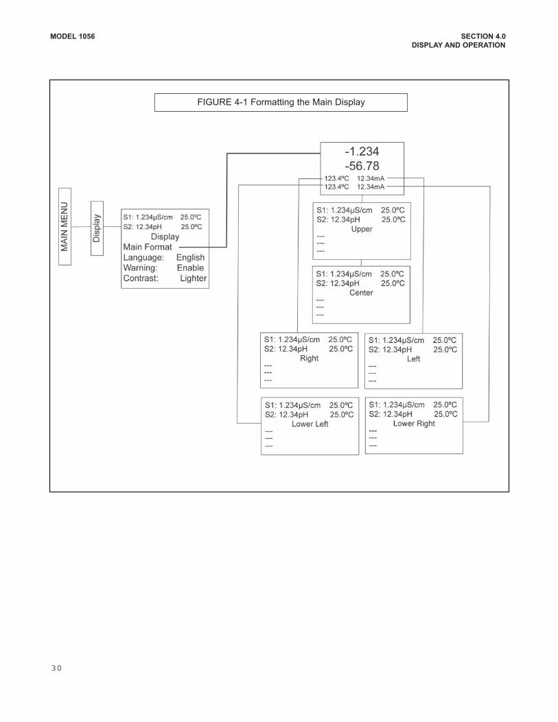
FIGURE 41 Formatting the Main Display
MODEL 1056 SECTION 4.0
DISPLAY AND OPERATION
30
MODEL 1056 SECTION 5.0
PROGRAMMING THE ANALYZER BASICS
SECTION 5.0.
PROGRAMMING THE ANALYZER BASICS
5.1 GENERALSection 5.0 describes the following programming functions:
Changing the measurement type, measurement units and temperature units. Choose temperature units and manual or automatic temperature compensation mode Configure and assign values to the current outputs Set a security code for two levels of security access Accessing menu functions using a security code Enabling and disabling Hold mode for current outputs Choosing the frequency of the AC power (needed for optimum noise rejection) Resetting all factory defaults, calibration data only, or current output settings only
5.2 CHANGING STARTUP SETTINGS5.2.1 PurposeTo change the measurement type, measurement units, or temperature units that were initially entered in QuickStart, choose the Reset analyzer function (Sec. 5.9) or access the Program menus for sensor 1 or sensor 2 (Sec.6.0). The following choices for specific measurement type, measurement units are available for each sensor measurement board.
Signal board Available measurements Measurements units:
pH/ORP (22, 32)pH, ORP, Redox, Ammonia, Fluoride,
Custom ISE
pH, mV (ORP)
%, ppm, mg/L, ppb, μg/L, (ISE)
Contacting conductivity
(20, 30)
Conductivity, Resistivity, TDS, Salinity,
NaOH (012%), HCl (015%), Low H2SO4,
High H2SO4, NaCl (020%),
Custom Curve
μS/cm, mS/cm, S/cm
% (concentration)
Toroidal conductivity
(21, 31)
Conductivity, Resistivity, TDS, Salinity,
NaOH (012%), HCl (015%), Low H2SO4,
High H2SO4, NaCl (020%),
Custom Curve
μS/cm, mS/cm, S/cm
% (concentration)
Chlorine
(24, 34)
Free Chlorine, pH Independ. Free Cl, Total
Chlorine, Monochloramineppm, mg/L
Oxygen
(25, 35)Oxygen (ppm), Trace Oxygen (ppb),
Percent Oxygen in gas, Salinity
ppm, mg/L, ppb, µg/L % Sat, Partial
Pressure, % Oxygen In Gas, ppm
Oxygen In Gas
Ozone (26, 36) Ozone ppm, mg/L, ppb, μg/L
Temperature (all) Temperature °C. ºF
5.2.2 Procedure.
Follow the Reset Analyzer procedure (Sec 5.8) to reconfigure the analyzer to display new measurements or
measurement units. To change the specific measurement or measurement units for each signal board type,
refer to the Program menu for the appropriate measurement (Sec. 6.0).
TABLE 51. Measurements and Measurement Units
5.1 GENERAL
5.2 CHANGING STARTUP SETTINGS
5.3 PROGRAMMING TEMPERATURE
5.4 CONFIGURING AND RANGING 420MA OUTPUTS
5.5 SETTING SECURITY CODES
5.6 SECURITY ACCESS
5.7 USING HOLD
5.8 RESETTING FACTORY DEFAULTS – RESET ANALYZER
5.9 PROGRAMMING ALARM RELAYS
31
MODEL 1056 SECTION 5.0
PROGRAMMING THE ANALYZER BASICS
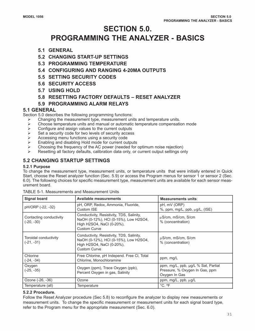
5.3.1 PurposeMost liquid analytical measurements (except ORP)require temperature compensation. The Model 1056performs temperature compensation automatically byapplying internal temperature correction algorithms.Temperature correction can also be turned off. If temperature correction is off, the Model 1056 uses the temperature entered by the user in all temperature correction calculations.
5.3.2 Procedure.Follow the menu screens in Fig. 5.1 to select automaticor manual temp compensation, set the manualreference temperature, and to program temperatureunits as °C or °F.
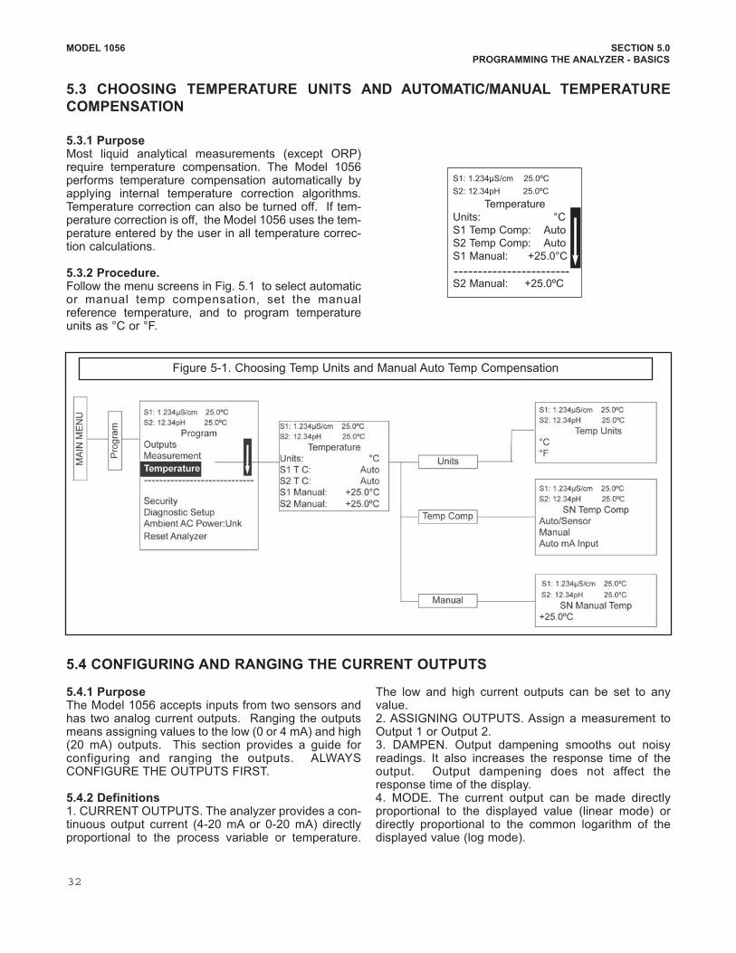
5.4.1 PurposeThe Model 1056 accepts inputs from two sensors andhas two analog current outputs. Ranging the outputsmeans assigning values to the low (0 or 4 mA) and high(20 mA) outputs. This section provides a guide forconfiguring and ranging the outputs. ALWAYSCONFIGURE THE OUTPUTS FIRST.
5.4.2 Definitions1. CURRENT OUTPUTS. The analyzer provides a continuous output current (420 mA or 020 mA) directlyproportional to the process variable or temperature.
The low and high current outputs can be set to anyvalue. 2. ASSIGNING OUTPUTS. Assign a measurement toOutput 1 or Output 2. 3. DAMPEN. Output dampening smooths out noisyreadings. It also increases the response time of theoutput. Output dampening does not affect theresponse time of the display.4. MODE. The current output can be made directlyproportional to the displayed value (linear mode) ordirectly proportional to the common logarithm of thedisplayed value (log mode).
S1: 1.234µS/cm 25.0ºC
S2: 12.34pH 25.0ºC
Temperature
Units: °C
S1 Temp Comp: Auto
S2 Temp Comp: Auto
S1 Manual: +25.0°C
S2 Manual: +25.0ºC
Figure 51. Choosing Temp Units and Manual Auto Temp Compensation
5.3 CHOOSING TEMPERATURE UNITS AND AUTOMATIC/MANUAL TEMPERATURE
COMPENSATION
5.4 CONFIGURING AND RANGING THE CURRENT OUTPUTS
32
MODEL 1056 SECTION 5.0
PROGRAMMING THE ANALYZER BASICS
5.4.3 Procedure: Configure Outputs.Under the Program/Outputs menu, the adjacent screenwill appear to allow configuration of the outputs. Followthe menu screens in Fig. 52 to configure the outputs.
5.4.4 Procedure: Assigning Measurements the Lowand High Current Outputs The adjacent screen will appear when entering theAssign function under Program/Output/Configure.These screens allow you to assign a measurement,process value, or temperature input to each output.Follow the menu screens in Fig. 52 to assignmeasurements to the outputs.
5.4.5 Procedure: Ranging the Current Outputs The adjacent screen will appear underProgram/Output/Range. Enter a value for 4mA and20mA (or 0mA and 20mA) for each output. Follow themenu screens in Fig. 52 to assign values to the outputs.
S1: 1.234µS/cm 25.0ºC
S2: 12.34pH 25.0ºC
OutputM Configure
Assign: S1 Meas
Range: 420mA
Scale: Linear
Dampening: 0sec
Fault Mode: Fixed
Fault Value: 21.00mA
S1: 1.234µS/cm 25.0ºC
S2: 12.34pH 25.0ºC
OutputM Assign
S1 Measurement
S1 Temperature
S2 Measurement
S2 Temperature
S1: 1.234µS/cm 25.0ºC
S2: 12.34pH 25.0ºC
Output Range
OM SN 4mA: 0.000µS/cm
OM SN 20mA: 20.00µS/cm
OM SN 4mA: 00.00pH
OM SN 20mA: 14.00pH
Figure 52. Configuring and Ranging the Current Outputs
33
Figure 53. Setting a Security Code
MA
IN M
EN
U S1: 1.234µS/cm 25.0ºC
S2: 12.34pH 25.0ºC
Program
Outputs
Measurement
Temperature
Diagnostic Setup
Ambient AC Power:Unk
Reset Analyzer
S1: 1.234µS/cm 25.0ºC
S2: 12.34pH 25.0ºC
Security
Calibration/Hold: 000
All: 000
Security
Pro
gra
m
MODEL 1056 SECTION 5.0
PROGRAMMING THE ANALYZER BASICS
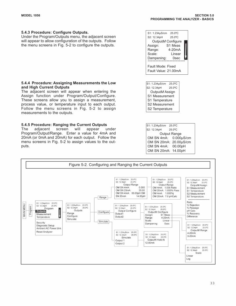
5.5 SETTING A SECURITY CODE
5.5.1 Purpose.The security codes prevent accidental or unwantedchanges to program settings, displays, and calibration.Model 1056 has two levels of security code to controlaccess and use of the instrument to different types ofusers. The two levels of security are:
All: This is the Supervisory security level. It allows access to all menu functions, includingProgramming, Calibration, Hold and Display.
Calibration/Hold: This is the operator ortechnician level menu. It allows access to
only calibration and Hold of the current outputs.
5.5.2 Procedure.1. Press MENU. The main menu screen appears.
Choose Program.
2. Scroll down to Security. Select Security. 3. The security entry screen appears. Enter a
three digit security code for each of the desiredsecurity levels. The security code takes effect
two minutes after the last key stroke.Record the security code(s) for future accessand communication to operators or technicians as needed.
4. The display returns to the security menu
screen. Press EXIT to return to the previous
screen. To return to the main display, press
MENU followed by EXIT.
Fig. 53 displays the security code screens.
34

MODEL 1056 SECTION 5.0
PROGRAMMING THE ANALYZER BASICS
5.6 SECURITY ACCESS
5.6.1 How the Security Code WorksWhen entering the correct access code for theCalibration/Hold security level, the Calibration andHold menus are accessible. This allows operators ortechnicians to perform routine maintenance. Thissecurity level does not allow access to the Program orDisplay menus. When entering the correct access code for All securitylevel, the user has access to all menu functions, including Programming, Calibration, Hold and Display.
5.6.2 Procedure.1. If a security code has been programmed, selecting
the Calibrate, Hold, Program or Display top menuitems causes the security access screen to appear
2. Enter the threedigit security code for the appropriatesecurity level.
3. If the entry is correct, the appropriate menu screen appears. If the entry is incorrect, the Invalid Codescreen appears. The Enter Security Code screen reappears after 2 seconds.
5.7 USING HOLD
5.7.1 PurposeThe analyzer output is always proportional to measuredvalue. To prevent improper operation of systems orpumps that are controlled directly by the currentoutput, place the analyzer in hold before removingthe sensor for calibration and maintenance. Be sureto remove the analyzer from hold once calibration iscomplete. During hold, both outputs remain at the lastvalue. Once in hold, all current outputs remain onHold indefinitely.
5.7.2 Using the Hold FunctionTo hold the outputs,
1. Press MENU. The main menu screen appears.Choose Hold.
2. The Hold Outputs and Alarms? screen appears. Choose Yes to place the analyzer in hold. Choose No to take the analyzer out of hold.Note: There are no alarm relays with this configuration. Current outputs are included with allconfigurations.
3. The Hold screen will then appear and Hold will remain on indefinitely until Hold isdisabled.
See figure 51 below.
S1: 1.234µS/cm 25.0ºC
S2: 12.34pH 25.0ºC
Security Code
000
MA
IN M
EN
U
Hold
S1: 1.234µS/cm 25.0ºC
S2: 12.34pH 25.0ºC
S1 Hold outputs
and alarms?
No
Yes
S1: 1.234µS/cm 25.0ºC
S2: 12.34pH 25.0ºC
Hold
S1 Hold: No
S2 Hold: No
Figure 54. Using Hold
35
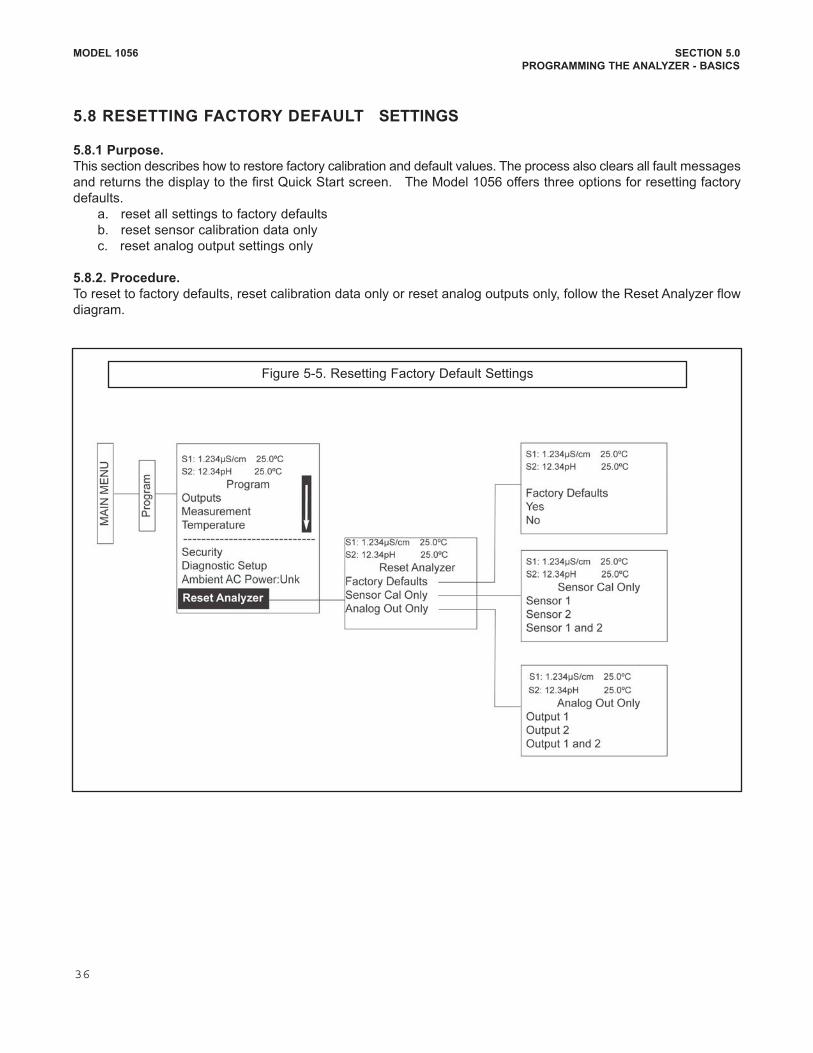
MODEL 1056 SECTION 5.0
PROGRAMMING THE ANALYZER BASICS
5.8 RESETTING FACTORY DEFAULT SETTINGS
5.8.1 Purpose.
This section describes how to restore factory calibration and default values. The process also clears all fault messages
and returns the display to the first Quick Start screen. The Model 1056 offers three options for resetting factory
defaults.
a. reset all settings to factory defaults
b. reset sensor calibration data only
c. reset analog output settings only
5.8.2. Procedure.
To reset to factory defaults, reset calibration data only or reset analog outputs only, follow the Reset Analyzer flow
diagram.
Figure 55. Resetting Factory Default Settings
36
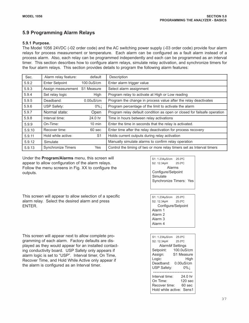
5.9 Programming Alarm Relays
5.9.1 Purpose.
The Model 1056 24VDC (02 order code) and the AC switching power supply (03 order code) provide four alarm
relays for process measurement or temperature. Each alarm can be configured as a fault alarm instead of a
process alarm. Also, each relay can be programmed independently and each can be programmed as an interval
timer. This section describes how to configure alarm relays, simulate relay activation, and synchronize timers for
the four alarm relays. This section provides details to program the following alarm features:
Under the Program/Alarms menu, this screen will
appear to allow configuration of the alarm relays.
Follow the menu screens in Fig. XX to configure the
outputs.
This screen will appear to allow selection of a specific
alarm relay. Select the desired alarm and press
ENTER.
This screen will appear next to allow complete pro
gramming of each alarm. Factory defaults are dis
played as they would appear for an installed contact
ing conductivity board. USP Safety only appears if
alarm logic is set to “USP”. Interval timer, On Time,
Recover Time, and Hold While Active only appear if
the alarm is configured as an Interval timer.
MODEL 1056 SECTION 5.0
PROGRAMMING THE ANALYZER BASICS
S1: 1.234µS/cm 25.0ºC
S2: 12.34pH 25.0ºC
Alarms
Configure/Setpoint
Simulate
Synchronize Timers: Yes
S1: 1.234µS/cm 25.0ºC
S2: 12.34pH 25.0ºC
Configure/Setpoint
Alarm 1
Alarm 2
Alarm 3
Alarm 4
S1: 1.234µS/cm 25.0ºC
S2: 12.34pH 25.0ºC
AlarmM Settings
Setpoint: 100.0uS/cm
Assign: S1 Measure
Logic: High
Deadband: 0.00uS/cm
USP Safety: 0%↓
Interval time: 24.0 hr
On Time: 120 sec
Recover time: 60 sec
Hold while active: Sens1
Sec. Alarm relay feature: default Description
5.9.2 Enter Setpoint 100.0uS/cm Enter alarm trigger value
5.9.3 Assign measurement S1 Measure Select alarm assignment
5.9.4 Set relay logic High Program relay to activate at High or Low reading
5.9.5 Deadband: 0.00uS/cm Program the change in process value after the relay deactivates
5.9.6 USP Safety: 0%↓ Program percentage of the limit to activate the alarm
5.9.7 Normal state: Open Program relay default condition as open or closed for failsafe operation
5.9.8 Interval time: 24.0 hr Time in hours between relay activations
5.9.9 OnTime: 10 min Enter the time in seconds that the relay is activated.
5.9.10 Recover time: 60 sec Enter time after the relay deactivation for process recovery
5.9.11 Hold while active: S1 Holds current outputs during relay activation
5.9.12 Simulate Manually simulate alarms to confirm relay operation
5.9.13 Synchronize Timers Yes Control the timing of two or more relay timers set as Interval timers
37
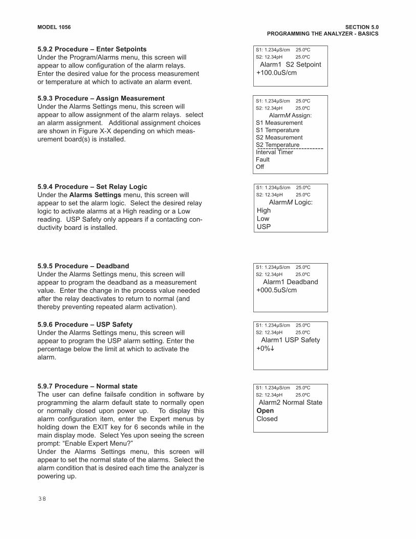
MODEL 1056 SECTION 5.0
PROGRAMMING THE ANALYZER BASICS
5.9.2 Procedure – Enter Setpoints
Under the Program/Alarms menu, this screen will
appear to allow configuration of the alarm relays.
Enter the desired value for the process measurement
or temperature at which to activate an alarm event.
5.9.3 Procedure – Assign Measurement
Under the Alarms Settings menu, this screen will
appear to allow assignment of the alarm relays. select
an alarm assignment. Additional assignment choices
are shown in Figure XX depending on which meas
urement board(s) is installed.
5.9.4 Procedure – Set Relay Logic
Under the Alarms Settings menu, this screen will
appear to set the alarm logic. Select the desired relay
logic to activate alarms at a High reading or a Low
reading. USP Safety only appears if a contacting con
ductivity board is installed.
5.9.5 Procedure – Deadband
Under the Alarms Settings menu, this screen will
appear to program the deadband as a measurement
value. Enter the change in the process value needed
after the relay deactivates to return to normal (and
thereby preventing repeated alarm activation).
5.9.6 Procedure – USP Safety
Under the Alarms Settings menu, this screen will
appear to program the USP alarm setting. Enter the
percentage below the limit at which to activate the
alarm.
5.9.7 Procedure – Normal state
The user can define failsafe condition in software by
programming the alarm default state to normally open
or normally closed upon power up. To display this
alarm configuration item, enter the Expert menus by
holding down the EXIT key for 6 seconds while in the
main display mode. Select Yes upon seeing the screen
prompt: “Enable Expert Menu?”
Under the Alarms Settings menu, this screen will
appear to set the normal state of the alarms. Select the
alarm condition that is desired each time the analyzer is
powering up.
S1: 1.234µS/cm 25.0ºC
S2: 12.34pH 25.0ºC
Alarm1 S2 Setpoint
+100.0uS/cm
S1: 1.234µS/cm 25.0ºC
S2: 12.34pH 25.0ºC
AlarmM Logic:
High
Low
USP
S1: 1.234µS/cm 25.0ºC
S2: 12.34pH 25.0ºC
Alarm1 Deadband
+000.5uS/cm
S1: 1.234µS/cm 25.0ºC
S2: 12.34pH 25.0ºC
Alarm1 USP Safety
+0%i
S1: 1.234µS/cm 25.0ºC
S2: 12.34pH 25.0ºC
Alarm2 Normal State
Open
Closed
S1: 1.234µS/cm 25.0ºC
S2: 12.34pH 25.0ºC
AlarmM Assign:
S1 Measurement
S1 Temperature
S2 Measurement
S2 Temperature
Interval Timer
Fault
Off
38
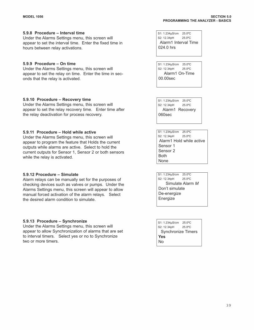
MODEL 1056 SECTION 5.0
PROGRAMMING THE ANALYZER BASICS
5.9.8 Procedure – Interval time
Under the Alarms Settings menu, this screen will
appear to set the interval time. Enter the fixed time in
hours between relay activations.
5.9.9 Procedure – On time
Under the Alarms Settings menu, this screen will
appear to set the relay on time. Enter the time in sec
onds that the relay is activated.
5.9.10 Procedure – Recovery time
Under the Alarms Settings menu, this screen will
appear to set the relay recovery time. Enter time after
the relay deactivation for process recovery.
5.9.11 Procedure – Hold while active
Under the Alarms Settings menu, this screen will
appear to program the feature that Holds the current
outputs while alarms are active. Select to hold the
current outputs for Sensor 1, Sensor 2 or both sensors
while the relay is activated.
5.9.12 Procedure – Simulate
Alarm relays can be manually set for the purposes of
checking devices such as valves or pumps. Under the
Alarms Settings menu, this screen will appear to allow
manual forced activation of the alarm relays. Select
the desired alarm condition to simulate.
5.9.13 Procedure – Synchronize
Under the Alarms Settings menu, this screen will
appear to allow Synchronization of alarms that are set
to interval timers. Select yes or no to Synchronize
two or more timers.
S1: 1.234µS/cm 25.0ºC
S2: 12.34pH 25.0ºC
Alarm1 Interval Time
024.0 hrs
S1: 1.234µS/cm 25.0ºC
S2: 12.34pH 25.0ºC
Alarm1 OnTime
00.00sec
S1: 1.234µS/cm 25.0ºC
S2: 12.34pH 25.0ºC
Alarm1 Recovery
060sec
S1: 1.234µS/cm 25.0ºC
S2: 12.34pH 25.0ºC
Synchronize Timers
Yes
No
S1: 1.234µS/cm 25.0ºC
S2: 12.34pH 25.0ºC
Alarm1 Hold while active
Sensor 1
Sensor 2
Both
None
S1: 1.234µS/cm 25.0ºC
S2: 12.34pH 25.0ºC
Simulate Alarm MDon’t simulate
Deenergize
Energize
39

This page left blank intentionally
MODEL 1056 SECTION 5.0
PROGRAMMING THE ANALYZER BASICS
40
MODEL 1056 SECTION 6.0
PROGRAMMING THE MEASUREMENTS
SECTION 6.0
PROGRAMMING MEASUREMENTS
6.1 CONFIGURING MEASUREMENTS – INTRODUCTION
6.2 pH
6.3 ORP
6.4 CONTACTING CONDUCTIVITY
6.5 TOROIDAL CONDUCTIVITY
6.6 CHLORINE
6.6.1 FREE CHLORINE
6.6.2 TOTAL CHLORINE
6.6.3 MONOCHLORAMINE
6.6.4 pHINDEPENDENT FREE CHLORINE
6.7 OXYGEN
6.8 OZONE
6.9 TURBIDITY
6.10 FLOW
6.11 CURRENT INPUT
6.1 PROGRAMMING MEASUREMENTS – INTRODUCTION The Model 1056 automatically recognizes each installed measurement board upon first powerup and each timethe analyzer is powered. Completion of Quick Start screens upon first power up enable measurements, but additional steps may be required to program the analyzer for the desired measurement application. This section covers the following programming and configuration functions;
1. Selecting measurement type or sensor type (all sections)2. Identifying the preamp location (pHsee Sec. 6.2)3. Enabling manual temperature correction and entering a reference temperature (all sections)4. Enabling sample temperature correction and entering temperature correction slope (selected sections)5. Defining measurement display resolution (pH and amperometric) 6. Defining measurement display units (all sections)7. Adjusting the input filter to control display and output reading variability or noise (all sections)8. Selecting a measurement range (conductivity – see Sec’s 6.4, 6.5) 9. Entering a cell constant for a contacting or toroidal sensor (see Sec’s 6.4, 6.5)
10. Entering a temperature element/RTD offset or temperature slope (conductivitysee Sec’s 6.4)11. Creating an applicationspecific concentration curve (conductivitysee Sec’s 6.4, 6.5)12. Enabling automatic pH correction for free chlorine measurement (Sec. 6.6.1)
To fully configure the analyzer for each installed measurement board, you may use the following: 1. Reset Analyzer function to reset factory defaults and configure the measurement board to the desired
measurement. Follow the Reset Analyzer menu (Fig. 55) to reconfigure the analyzer to display new measurements or measurement units.
2. Program menus to adjust any of the programmable configuration items. Use the following configurationand programming guidelines for the applicable measurement.
41
MODEL 1056 SECTION 6.0
PROGRAMMING THE MEASUREMENTS
6.2 pH MEASUREMENT PROGRAMMING
6.2.1 Description
This section describes how to configure the Model 1056 analyzer for pH measurements. The following programming and
configuration functions are covered.
Measure Sec. Menu function: default setting Description
pH 6.2.2 Measurement type: pH Select pH, ORP, Redox, Ammonia, Fluoride, Custom ISE
6.2.3 Preamp location: Analyzer Identify preamp location
6.2.4 Solution temperature correction Off Select Off, ultrapure, high pH, custom
6.2.5 Temp coefficient (custom) Enter the temp coefficient
6.2.6 Resolution: 0.01pH Select 0.01pH or 0.1pH for pH display resolution
6.2.7 Filter: 4 sec Override the default input filter, enter 0999 seconds
6.2.8 Reference Z: Low Select low or high reference impedance
To configure the pH measurement board:
1. Press MENU
2. Scroll down to Program. Press ENTER.
3. Scroll down to Measurement. Press ENTER.
4. Select Sensor 1 or Sensor 2 corresponding to
pH. Press ENTER.
The adjacent screen format will appear (factory defaults
are shown). To program any function, scroll to the
desired item and press ENTER.
6.2.2 Measurement
The display screen for selecting the measurement is
shown. The default value is displayed in bold type.
Refer to the pH/ORP Programming flow diagram to
complete this function.
S1: 1.234µS/cm 25.0ºC
S2: 12.34pH 25.0ºC
SN Configure
Measure: pH
Preamp: Analyzer
Sol’n Temp Corr: Off
T Coeff: 0.029pH/°C
Resolution: 0.01pH
Filter: 4 sec
Reference Z: Low
S1: 1.234µS/cm 25.0ºC
S2: 12.34pH 25.0ºC
SN Measurement
pH
ORP
Redox
Ammonia
Fluoride
Custom ISE
The following subsections provide you with the initial display screen that appears for each configuration function.
Use the flow diagram for pH programming at the end of Sec. 6 and the Model 1056 live screen prompts for each
function to complete configuration and programming.
6.2.3 Preamp
The display screen for identifying the Preamp location is
shown. The default value is displayed in bold type.
Refer to the pH/ORP Programming flow diagram to
complete this function.
S1: 1.234µS/cm 25.0ºC
S2: 12.34pH 25.0ºC
SN Preamp
Analyzer
Sensor/JBox
TABLE 61. pH Measurement Programming
A detailed flow diagram for pH programming is provided at the end of Sec. 6 to guide you through
all basic programming and configuration functions.
42
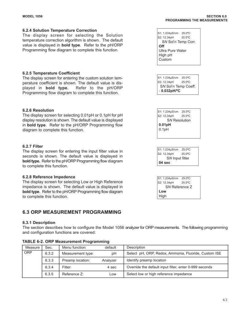
MODEL 1056 SECTION 6.0
PROGRAMMING THE MEASUREMENTS
6.2.4 Solution Temperature Correction
The display screen for selecting the Solution
temperature correction algorithm is shown. The default
value is displayed in bold type. Refer to the pH/ORP
Programming flow diagram to complete this function.
6.2.5 Temperature Coefficient
The display screen for entering the custom solution tem
perature coefficient is shown. The default value is dis
played in bold type. Refer to the pH/ORP
Programming flow diagram to complete this function.
6.2.6 Resolution
The display screen for selecting 0.01pH or 0.1pH for pH
display resolution is shown. The default value is displayed
in bold type. Refer to the pH/ORP Programming flow
diagram to complete this function.
S1: 1.234µS/cm 25.0ºC
S2: 12.34pH 25.0ºC
SN Sol’n Temp Corr.
Off
Ultra Pure Water
High pH
Custom
S1: 1.234µS/cm 25.0ºC
S2: 12.34pH 25.0ºC
SN Resolution
0.01pH
0.1pH
S1: 1.234µS/cm 25.0ºC
S2: 12.34pH 25.0ºC
SN Sol’n Temp Coeff.
0.032pH/ºC
6.2.7 Filter
The display screen for entering the input filter value in
seconds is shown. The default value is displayed in
bold type. Refer to the pH/ORP Programming flow diagram
to complete this function.
6.2.8 Reference Impedence
The display screen for selecting Low or High Reference
impedance is shown. The default value is displayed in
bold type. Refer to the pH/ORP Programming flow diagram
to complete this function.
S1: 1.234µS/cm 25.0ºC
S2: 12.34pH 25.0ºC
SN Reference Z
Low
High
S1: 1.234µS/cm 25.0ºC
S2: 12.34pH 25.0ºC
SN Input filter
04 sec
6.3 ORP MEASUREMENT PROGRAMMING
6.3.1 Description
The section describes how to configure the Model 1056 analyzer for ORP measurements. The following programming
and configuration functions are covered:
Measure Sec. Menu function: default Description
ORP 6.3.2 Measurement type: pH Select pH, ORP, Redox, Ammonia, Fluoride, Custom ISE
6.3.3 Preamp location: Analyzer Identify preamp location
6.3.4 Filter: 4 sec Override the default input filter, enter 0999 seconds
6.3.5 Reference Z: Low Select low or high reference impedance
TABLE 62. ORP Measurement Programming
43
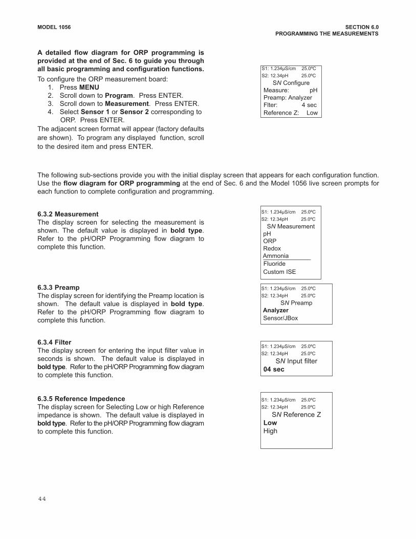
MODEL 1056 SECTION 6.0
PROGRAMMING THE MEASUREMENTS
The following subsections provide you with the initial display screen that appears for each configuration function.
Use the flow diagram for ORP programming at the end of Sec. 6 and the Model 1056 live screen prompts for
each function to complete configuration and programming.
6.3.2 Measurement
The display screen for selecting the measurement is
shown. The default value is displayed in bold type.
Refer to the pH/ORP Programming flow diagram to
complete this function.
6.3.3 Preamp
The display screen for identifying the Preamp location is
shown. The default value is displayed in bold type.
Refer to the pH/ORP Programming flow diagram to
complete this function.
6.3.4 Filter
The display screen for entering the input filter value in
seconds is shown. The default value is displayed in
bold type. Refer to the pH/ORP Programming flow diagram
to complete this function.
A detailed flow diagram for ORP programming is
provided at the end of Sec. 6 to guide you through
all basic programming and configuration functions.
To configure the ORP measurement board:
1. Press MENU
2. Scroll down to Program. Press ENTER.
3. Scroll down to Measurement. Press ENTER.
4. Select Sensor 1 or Sensor 2 corresponding to
ORP. Press ENTER.
The adjacent screen format will appear (factory defaults
are shown). To program any displayed function, scroll
to the desired item and press ENTER.
S1: 1.234µS/cm 25.0ºC
S2: 12.34pH 25.0ºC
SN Preamp
Analyzer
Sensor/JBox
S1: 1.234µS/cm 25.0ºC
S2: 12.34pH 25.0ºC
SN Input filter
04 sec
6.3.5 Reference Impedence
The display screen for Selecting Low or high Reference
impedance is shown. The default value is displayed in
bold type. Refer to the pH/ORP Programming flow diagram
to complete this function.
S1: 1.234µS/cm 25.0ºC
S2: 12.34pH 25.0ºC
SN Reference Z
Low
High
S1: 1.234µS/cm 25.0ºC
S2: 12.34pH 25.0ºC
SN Configure
Measure: pH
Preamp: Analyzer
Flter: 4 sec
Reference Z: Low
44
S1: 1.234µS/cm 25.0ºC
S2: 12.34pH 25.0ºC
SN Measurement
pH
ORP
Redox
Ammonia
Fluoride
Custom ISE
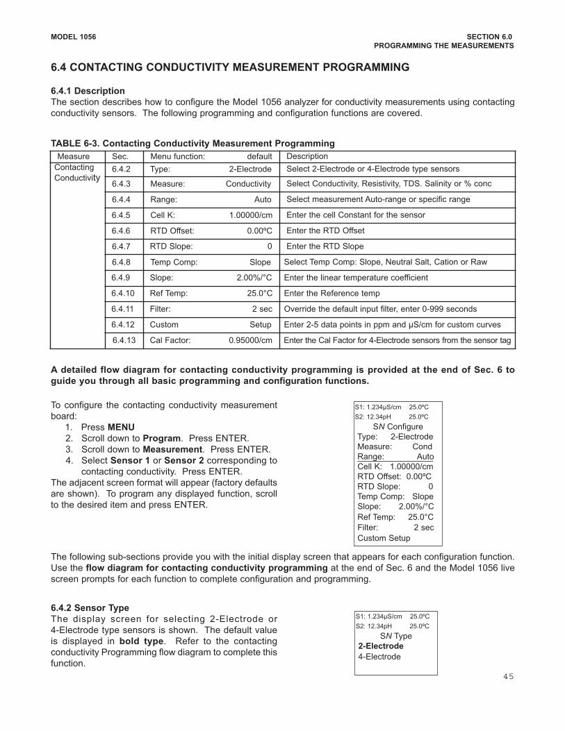
6.4.2 Sensor Type
The display screen for selecting 2Electrode or
4Electrode type sensors is shown. The default value
is displayed in bold type. Refer to the contacting
conductivity Programming flow diagram to complete this
function.
MODEL 1056 SECTION 6.0
PROGRAMMING THE MEASUREMENTS
6.4 CONTACTING CONDUCTIVITY MEASUREMENT PROGRAMMING
6.4.1 Description
The section describes how to configure the Model 1056 analyzer for conductivity measurements using contacting
conductivity sensors. The following programming and configuration functions are covered.
The following subsections provide you with the initial display screen that appears for each configuration function.
Use the flow diagram for contacting conductivity programming at the end of Sec. 6 and the Model 1056 live
screen prompts for each function to complete configuration and programming.
To configure the contacting conductivity measurement
board:
1. Press MENU
2. Scroll down to Program. Press ENTER.
3. Scroll down to Measurement. Press ENTER.
4. Select Sensor 1 or Sensor 2 corresponding to
contacting conductivity. Press ENTER.
The adjacent screen format will appear (factory defaults
are shown). To program any displayed function, scroll
to the desired item and press ENTER.
Measure Sec. Menu function: default Description
Contacting
Conductivity6.4.2 Type: 2Electrode Select 2Electrode or 4Electrode type sensors
6.4.3 Measure: Conductivity Select Conductivity, Resistivity, TDS. Salinity or % conc
6.4.4 Range: Auto Select measurement Autorange or specific range
6.4.5 Cell K: 1.00000/cm Enter the cell Constant for the sensor
6.4.6 RTD Offset: 0.00ºC Enter the RTD Offset
6.4.7 RTD Slope: 0 Enter the RTD Slope
6.4.8 Temp Comp: Slope Select Temp Comp: Slope, Neutral Salt, Cation or Raw
6.4.9 Slope: 2.00%/°C Enter the linear temperature coefficient
6.4.10 Ref Temp: 25.0°C Enter the Reference temp
6.4.11 Filter: 2 sec Override the default input filter, enter 0999 seconds
6.4.12 Custom Setup Enter 25 data points in ppm and µS/cm for custom curves
6.4.13 Cal Factor: 0.95000/cm Enter the Cal Factor for 4Electrode sensors from the sensor tag
S1: 1.234µS/cm 25.0ºC
S2: 12.34pH 25.0ºC
SN Configure
Type: 2Electrode
Measure: Cond
Range: Auto
Cell K: 1.00000/cm
RTD Offset: 0.00ºC
RTD Slope: 0
Temp Comp: Slope
Slope: 2.00%/°C
Ref Temp: 25.0°C
Filter: 2 sec
Custom Setup
S1: 1.234µS/cm 25.0ºC
S2: 12.34pH 25.0ºC
SN Type
2Electrode
4Electrode
TABLE 63. Contacting Conductivity Measurement Programming
A detailed flow diagram for contacting conductivity programming is provided at the end of Sec. 6 to
guide you through all basic programming and configuration functions.
45
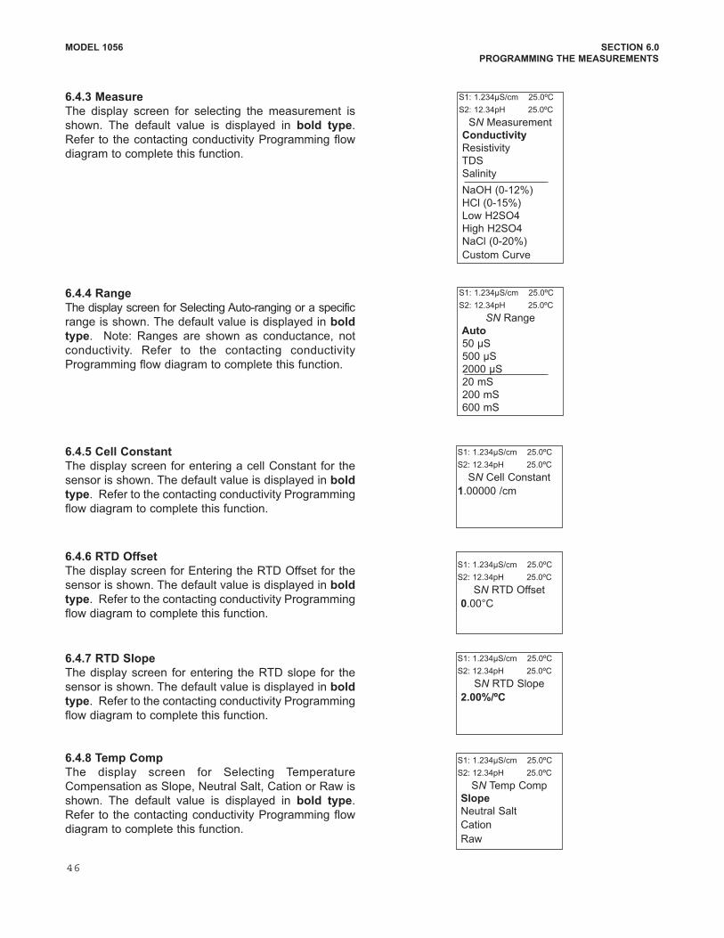
MODEL 1056 SECTION 6.0
PROGRAMMING THE MEASUREMENTS
6.4.3 Measure
The display screen for selecting the measurement is
shown. The default value is displayed in bold type.
Refer to the contacting conductivity Programming flow
diagram to complete this function.
6.4.4 Range
The display screen for Selecting Autoranging or a specific
range is shown. The default value is displayed in bold
type. Note: Ranges are shown as conductance, not
conductivity. Refer to the contacting conductivity
Programming flow diagram to complete this function.
S1: 1.234µS/cm 25.0ºC
S2: 12.34pH 25.0ºC
SN Measurement
Conductivity
Resistivity
TDS
Salinity
NaOH (012%)
HCl (015%)
Low H2SO4
High H2SO4
NaCl (020%)
Custom Curve
S1: 1.234µS/cm 25.0ºC
S2: 12.34pH 25.0ºC
SN Range
Auto
50 µS
500 µS
2000 µS
20 mS
200 mS
600 mS
6.4.5 Cell Constant
The display screen for entering a cell Constant for the
sensor is shown. The default value is displayed in bold
type. Refer to the contacting conductivity Programming
flow diagram to complete this function.
S1: 1.234µS/cm 25.0ºC
S2: 12.34pH 25.0ºC
SN Cell Constant
1.00000 /cm
6.4.6 RTD Offset
The display screen for Entering the RTD Offset for the
sensor is shown. The default value is displayed in bold
type. Refer to the contacting conductivity Programming
flow diagram to complete this function.
S1: 1.234µS/cm 25.0ºC
S2: 12.34pH 25.0ºC
SN RTD Offset
0.00°C
6.4.7 RTD Slope
The display screen for entering the RTD slope for the
sensor is shown. The default value is displayed in bold
type. Refer to the contacting conductivity Programming
flow diagram to complete this function.
S1: 1.234µS/cm 25.0ºC
S2: 12.34pH 25.0ºC
SN RTD Slope
2.00%/ºC
6.4.8 Temp Comp
The display screen for Selecting Temperature
Compensation as Slope, Neutral Salt, Cation or Raw is
shown. The default value is displayed in bold type.
Refer to the contacting conductivity Programming flow
diagram to complete this function.
S1: 1.234µS/cm 25.0ºC
S2: 12.34pH 25.0ºC
SN Temp Comp
Slope
Neutral Salt
Cation
Raw
46
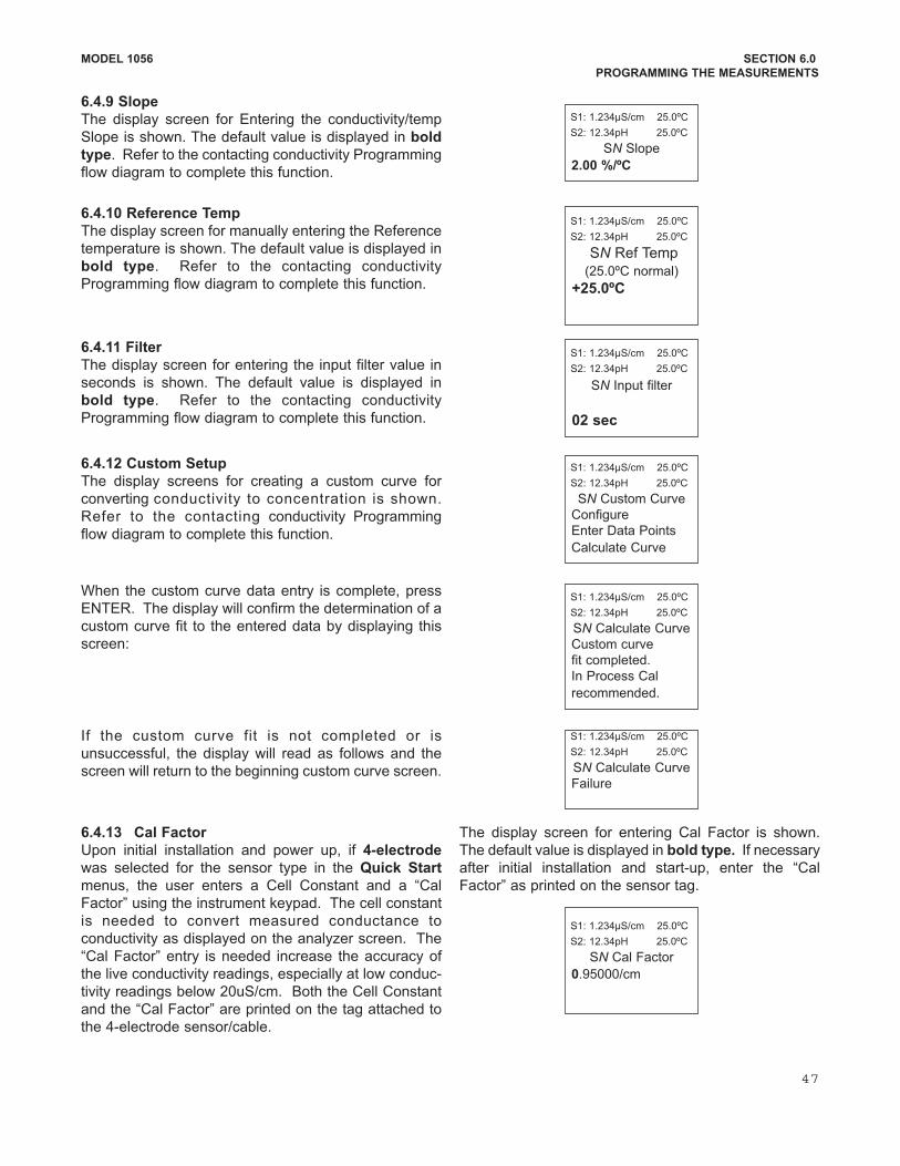
6.4.13 Cal Factor
Upon initial installation and power up, if 4electrode
was selected for the sensor type in the Quick Start
menus, the user enters a Cell Constant and a “Cal
Factor” using the instrument keypad. The cell constant
is needed to convert measured conductance to
conductivity as displayed on the analyzer screen. The
“Cal Factor” entry is needed increase the accuracy of
the live conductivity readings, especially at low conduc
tivity readings below 20uS/cm. Both the Cell Constant
and the “Cal Factor” are printed on the tag attached to
the 4electrode sensor/cable.
The display screen for entering Cal Factor is shown.
The default value is displayed in bold type. If necessary
after initial installation and startup, enter the “Cal
Factor” as printed on the sensor tag.
MODEL 1056 SECTION 6.0
PROGRAMMING THE MEASUREMENTS
6.4.9 Slope
The display screen for Entering the conductivity/temp
Slope is shown. The default value is displayed in bold
type. Refer to the contacting conductivity Programming
flow diagram to complete this function.
S1: 1.234µS/cm 25.0ºC
S2: 12.34pH 25.0ºC
SN Slope
2.00 %/ºC
6.4.10 Reference Temp
The display screen for manually entering the Reference
temperature is shown. The default value is displayed in
bold type. Refer to the contacting conductivity
Programming flow diagram to complete this function.
S1: 1.234µS/cm 25.0ºC
S2: 12.34pH 25.0ºC
SN Ref Temp
(25.0ºC normal)
+25.0ºC
6.4.11 Filter
The display screen for entering the input filter value in
seconds is shown. The default value is displayed in
bold type. Refer to the contacting conductivity
Programming flow diagram to complete this function.
S1: 1.234µS/cm 25.0ºC
S2: 12.34pH 25.0ºC
SN Input filter
02 sec
6.4.12 Custom Setup
The display screens for creating a custom curve for
converting conductivity to concentration is shown.
Refer to the contacting conductivity Programming
flow diagram to complete this function.
S1: 1.234µS/cm 25.0ºC
S2: 12.34pH 25.0ºC
SN Custom Curve
Configure
Enter Data Points
Calculate Curve
S1: 1.234µS/cm 25.0ºC
S2: 12.34pH 25.0ºC
SN Cal Factor
0.95000/cm
When the custom curve data entry is complete, press
ENTER. The display will confirm the determination of a
custom curve fit to the entered data by displaying this
screen:
S1: 1.234µS/cm 25.0ºC
S2: 12.34pH 25.0ºC
SN Calculate Curve
Custom curve
fit completed.
In Process Cal
recommended.
If the custom curve fit is not completed or is
unsuccessful, the display will read as follows and the
screen will return to the beginning custom curve screen.
S1: 1.234µS/cm 25.0ºC
S2: 12.34pH 25.0ºC
SN Calculate Curve
Failure
47
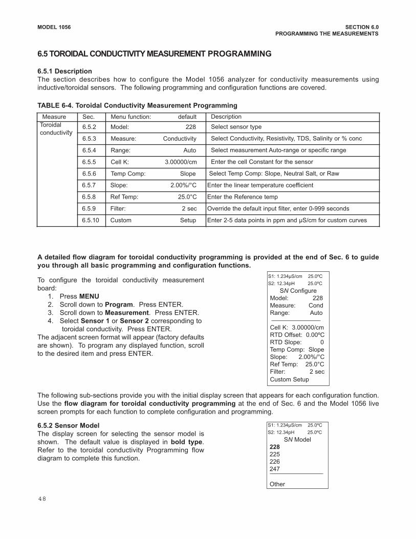
MODEL 1056 SECTION 6.0
PROGRAMMING THE MEASUREMENTS
6.5 TOROIDAL CONDUCTIVITY MEASUREMENT PROGRAMMING
6.5.1 Description
The section describes how to configure the Model 1056 analyzer for conductivity measurements using
inductive/toroidal sensors. The following programming and configuration functions are covered.
Measure Sec. Menu function: default Description
Toroidal
conductivity6.5.2 Model: 228 Select sensor type
6.5.3 Measure: Conductivity Select Conductivity, Resistivity, TDS, Salinity or % conc
6.5.4 Range: Auto Select measurement Autorange or specific range
6.5.5 Cell K: 3.00000/cm Enter the cell Constant for the sensor
6.5.6 Temp Comp: Slope Select Temp Comp: Slope, Neutral Salt, or Raw
6.5.7 Slope: 2.00%/°C Enter the linear temperature coefficient
6.5.8 Ref Temp: 25.0°C Enter the Reference temp
6.5.9 Filter: 2 sec Override the default input filter, enter 0999 seconds
6.5.10 Custom Setup Enter 25 data points in ppm and µS/cm for custom curves
To configure the toroidal conductivity measurement
board:
1. Press MENU
2. Scroll down to Program. Press ENTER.
3. Scroll down to Measurement. Press ENTER.
4. Select Sensor 1 or Sensor 2 corresponding to
toroidal conductivity. Press ENTER.
The adjacent screen format will appear (factory defaults
are shown). To program any displayed function, scroll
to the desired item and press ENTER.
The following subsections provide you with the initial display screen that appears for each configuration function.
Use the flow diagram for toroidal conductivity programming at the end of Sec. 6 and the Model 1056 live
screen prompts for each function to complete configuration and programming.
S1: 1.234µS/cm 25.0ºC
S2: 12.34pH 25.0ºC
SN Configure
Model: 228
Measure: Cond
Range: Auto
Cell K: 3.00000/cm
RTD Offset: 0.00ºC
RTD Slope: 0
Temp Comp: Slope
Slope: 2.00%/°C
Ref Temp: 25.0°C
Filter: 2 sec
Custom Setup
6.5.2 Sensor Model
The display screen for selecting the sensor model is
shown. The default value is displayed in bold type.
Refer to the toroidal conductivity Programming flow
diagram to complete this function.
S1: 1.234µS/cm 25.0ºC
S2: 12.34pH 25.0ºC
SN Model
228
225
226
247
Other
TABLE 64. Toroidal Conductivity Measurement Programming
A detailed flow diagram for toroidal conductivity programming is provided at the end of Sec. 6 to guide
you through all basic programming and configuration functions.
48
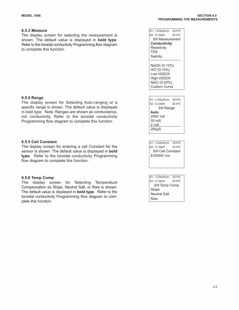
MODEL 1056 SECTION 6.0
PROGRAMMING THE MEASUREMENTS
6.5.3 Measure
The display screen for selecting the measurement is
shown. The default value is displayed in bold type.
Refer to the toroidal conductivity Programming flow diagram
to complete this function.
6.5.4 Range
The display screen for Selecting Autoranging or a
specific range is shown. The default value is displayed
in bold type. Note: Ranges are shown as conductance,
not conductivity. Refer to the toroidal conductivity
Programming flow diagram to complete this function.
6.5.5 Cell Constant
The display screen for entering a cell Constant for the
sensor is shown. The default value is displayed in bold
type. Refer to the toroidal conductivity Programming
flow diagram to complete this function.
S1: 1.234µS/cm 25.0ºC
S2: 12.34pH 25.0ºC
SN Cell Constant
3.00000 /cm
S1: 1.234µS/cm 25.0ºC
S2: 12.34pH 25.0ºC
SN Measurement
Conductivity
Resistivity
TDS
Salinity
NaOH (012%)
HCl (015%)
Low H2SO4
High H2SO4
NaCl (020%)
Custom Curve
S1: 1.234µS/cm 25.0ºC
S2: 12.34pH 25.0ºC
SN Range
Auto
2000 mS
50 mS
2 mS
200µS
6.5.6 Temp Comp
The display screen for Selecting Temperature
Compensation as Slope, Neutral Salt, or Raw is shown.
The default value is displayed in bold type. Refer to the
toroidal conductivity Programming flow diagram to com
plete this function.
S1: 1.234µS/cm 25.0ºC
S2: 12.34pH 25.0ºC
SN Temp Comp
Slope
Neutral Salt
Raw
49
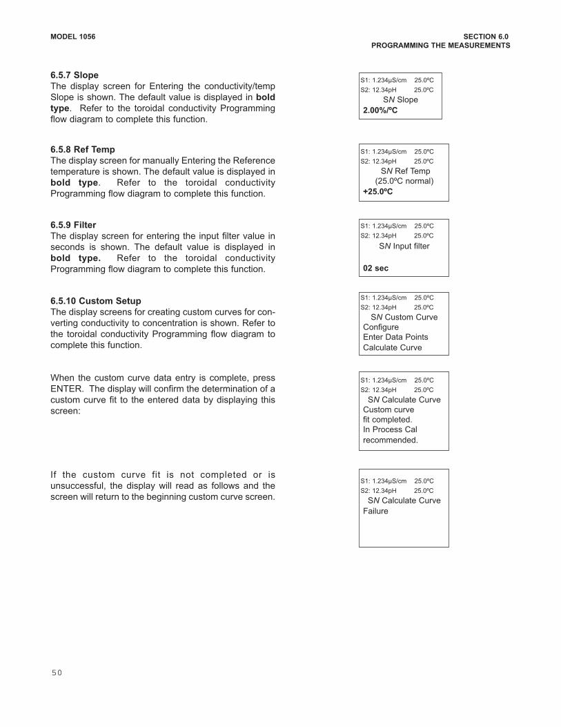
MODEL 1056 SECTION 6.0
PROGRAMMING THE MEASUREMENTS
6.5.7 Slope
The display screen for Entering the conductivity/temp
Slope is shown. The default value is displayed in bold
type. Refer to the toroidal conductivity Programming
flow diagram to complete this function.
S1: 1.234µS/cm 25.0ºC
S2: 12.34pH 25.0ºC
SN Slope
2.00%/ºC
6.5.8 Ref Temp
The display screen for manually Entering the Reference
temperature is shown. The default value is displayed in
bold type. Refer to the toroidal conductivity
Programming flow diagram to complete this function.
S1: 1.234µS/cm 25.0ºC
S2: 12.34pH 25.0ºC
SN Ref Temp
(25.0ºC normal)
+25.0ºC
6.5.9 Filter
The display screen for entering the input filter value in
seconds is shown. The default value is displayed in
bold type. Refer to the toroidal conductivity
Programming flow diagram to complete this function.
S1: 1.234µS/cm 25.0ºC
S2: 12.34pH 25.0ºC
SN Input filter
02 sec
6.5.10 Custom Setup
The display screens for creating custom curves for con
verting conductivity to concentration is shown. Refer to
the toroidal conductivity Programming flow diagram to
complete this function.
S1: 1.234µS/cm 25.0ºC
S2: 12.34pH 25.0ºC
SN Custom Curve
Configure
Enter Data Points
Calculate Curve
When the custom curve data entry is complete, press
ENTER. The display will confirm the determination of a
custom curve fit to the entered data by displaying this
screen:
S1: 1.234µS/cm 25.0ºC
S2: 12.34pH 25.0ºC
SN Calculate Curve
Custom curve
fit completed.
In Process Cal
recommended.
If the custom curve fit is not completed or is
unsuccessful, the display will read as follows and the
screen will return to the beginning custom curve screen.
S1: 1.234µS/cm 25.0ºC
S2: 12.34pH 25.0ºC
SN Calculate Curve
Failure
50
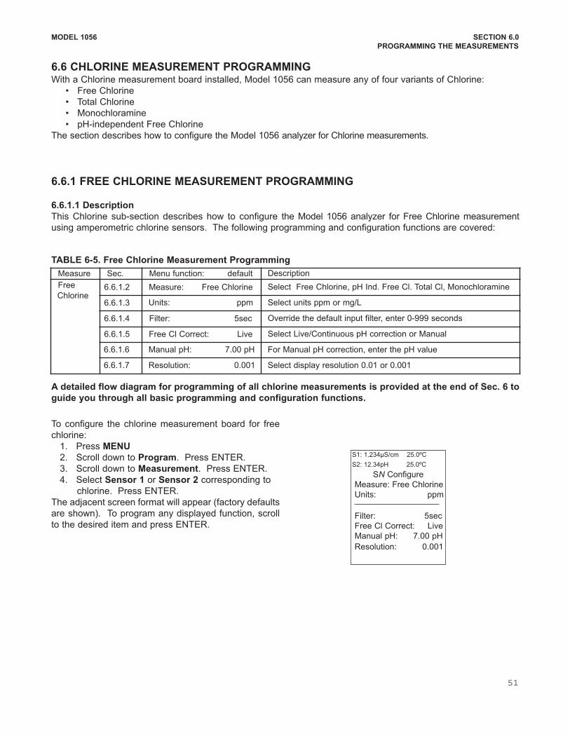
MODEL 1056 SECTION 6.0
PROGRAMMING THE MEASUREMENTS
6.6 CHLORINE MEASUREMENT PROGRAMMINGWith a Chlorine measurement board installed, Model 1056 can measure any of four variants of Chlorine:
• Free Chlorine
• Total Chlorine
• Monochloramine
• pHindependent Free Chlorine
The section describes how to configure the Model 1056 analyzer for Chlorine measurements.
6.6.1 FREE CHLORINE MEASUREMENT PROGRAMMING
6.6.1.1 Description
This Chlorine subsection describes how to configure the Model 1056 analyzer for Free Chlorine measurement
using amperometric chlorine sensors. The following programming and configuration functions are covered:
To configure the chlorine measurement board for free
chlorine:
1. Press MENU
2. Scroll down to Program. Press ENTER.
3. Scroll down to Measurement. Press ENTER.
4. Select Sensor 1 or Sensor 2 corresponding to
chlorine. Press ENTER.
The adjacent screen format will appear (factory defaults
are shown). To program any displayed function, scroll
to the desired item and press ENTER.
Measure Sec. Menu function: default Description
Free
Chlorine6.6.1.2 Measure: Free Chlorine Select Free Chlorine, pH Ind. Free Cl. Total Cl, Monochloramine
6.6.1.3 Units: ppm Select units ppm or mg/L
6.6.1.4 Filter: 5sec Override the default input filter, enter 0999 seconds
6.6.1.5 Free Cl Correct: Live Select Live/Continuous pH correction or Manual
6.6.1.6 Manual pH: 7.00 pH For Manual pH correction, enter the pH value
6.6.1.7 Resolution: 0.001 Select display resolution 0.01 or 0.001
S1: 1.234µS/cm 25.0ºC
S2: 12.34pH 25.0ºC
SN Configure
Measure: Free Chlorine
Units: ppm
Filter: 5sec
Free Cl Correct: Live
Manual pH: 7.00 pH
Resolution: 0.001
TABLE 65. Free Chlorine Measurement Programming
A detailed flow diagram for programming of all chlorine measurements is provided at the end of Sec. 6 to
guide you through all basic programming and configuration functions.
51
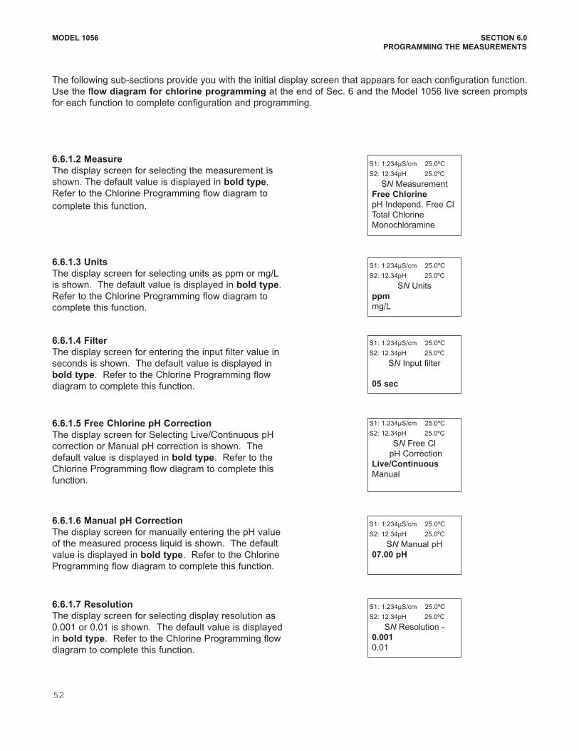
MODEL 1056 SECTION 6.0
PROGRAMMING THE MEASUREMENTS
The following subsections provide you with the initial display screen that appears for each configuration function.
Use the flow diagram for chlorine programming at the end of Sec. 6 and the Model 1056 live screen prompts
for each function to complete configuration and programming.
6.6.1.2 Measure
The display screen for selecting the measurement is
shown. The default value is displayed in bold type.
Refer to the Chlorine Programming flow diagram to
complete this function.
S1: 1.234µS/cm 25.0ºC
S2: 12.34pH 25.0ºC
SN Measurement
Free Chlorine
pH Independ. Free Cl
Total Chlorine
Monochloramine
6.6.1.3 Units
The display screen for selecting units as ppm or mg/L
is shown. The default value is displayed in bold type.
Refer to the Chlorine Programming flow diagram to
complete this function.
S1: 1.234µS/cm 25.0ºC
S2: 12.34pH 25.0ºC
SN Units
ppm
mg/L
6.6.1.4 Filter
The display screen for entering the input filter value in
seconds is shown. The default value is displayed in
bold type. Refer to the Chlorine Programming flow
diagram to complete this function.
S1: 1.234µS/cm 25.0ºC
S2: 12.34pH 25.0ºC
SN Input filter
05 sec
6.6.1.6 Manual pH Correction
The display screen for manually entering the pH value
of the measured process liquid is shown. The default
value is displayed in bold type. Refer to the Chlorine
Programming flow diagram to complete this function.
S1: 1.234µS/cm 25.0ºC
S2: 12.34pH 25.0ºC
SN Manual pH
07.00 pH
6.6.1.7 Resolution
The display screen for selecting display resolution as
0.001 or 0.01 is shown. The default value is displayed
in bold type. Refer to the Chlorine Programming flow
diagram to complete this function.
S1: 1.234µS/cm 25.0ºC
S2: 12.34pH 25.0ºC
SN Resolution
0.001
0.01
6.6.1.5 Free Chlorine pH Correction
The display screen for Selecting Live/Continuous pH
correction or Manual pH correction is shown. The
default value is displayed in bold type. Refer to the
Chlorine Programming flow diagram to complete this
function.
S1: 1.234µS/cm 25.0ºC
S2: 12.34pH 25.0ºC
SN Free Cl
pH Correction
Live/Continuous
Manual
52
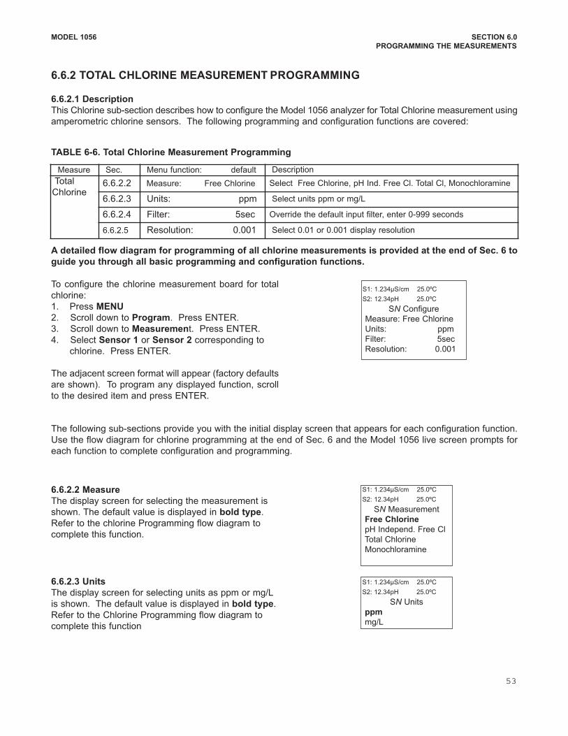
MODEL 1056 SECTION 6.0
PROGRAMMING THE MEASUREMENTS
6.6.2.2 Measure
The display screen for selecting the measurement is
shown. The default value is displayed in bold type.
Refer to the chlorine Programming flow diagram to
complete this function.
S1: 1.234µS/cm 25.0ºC
S2: 12.34pH 25.0ºC
SN Measurement
Free Chlorine
pH Independ. Free Cl
Total Chlorine
Monochloramine
6.6.2.3 Units
The display screen for selecting units as ppm or mg/L
is shown. The default value is displayed in bold type.
Refer to the Chlorine Programming flow diagram to
complete this function
S1: 1.234µS/cm 25.0ºC
S2: 12.34pH 25.0ºC
SN Units
ppm
mg/L
6.6.2 TOTAL CHLORINE MEASUREMENT PROGRAMMING
6.6.2.1 Description
This Chlorine subsection describes how to configure the Model 1056 analyzer for Total Chlorine measurement using
amperometric chlorine sensors. The following programming and configuration functions are covered:
Measure Sec. Menu function: default Description
Total
Chlorine6.6.2.2 Measure: Free Chlorine Select Free Chlorine, pH Ind. Free Cl. Total Cl, Monochloramine
6.6.2.3 Units: ppm Select units ppm or mg/L
6.6.2.4 Filter: 5sec Override the default input filter, enter 0999 seconds
6.6.2.5 Resolution: 0.001 Select 0.01 or 0.001 display resolution
To configure the chlorine measurement board for total
chlorine:
1. Press MENU
2. Scroll down to Program. Press ENTER.
3. Scroll down to Measurement. Press ENTER.
4. Select Sensor 1 or Sensor 2 corresponding to
chlorine. Press ENTER.
The adjacent screen format will appear (factory defaults
are shown). To program any displayed function, scroll
to the desired item and press ENTER.
S1: 1.234µS/cm 25.0ºC
S2: 12.34pH 25.0ºC
SN Configure
Measure: Free Chlorine
Units: ppm
Filter: 5sec
Resolution: 0.001
The following subsections provide you with the initial display screen that appears for each configuration function.
Use the flow diagram for chlorine programming at the end of Sec. 6 and the Model 1056 live screen prompts for
each function to complete configuration and programming.
TABLE 66. Total Chlorine Measurement Programming
A detailed flow diagram for programming of all chlorine measurements is provided at the end of Sec. 6 to
guide you through all basic programming and configuration functions.
53
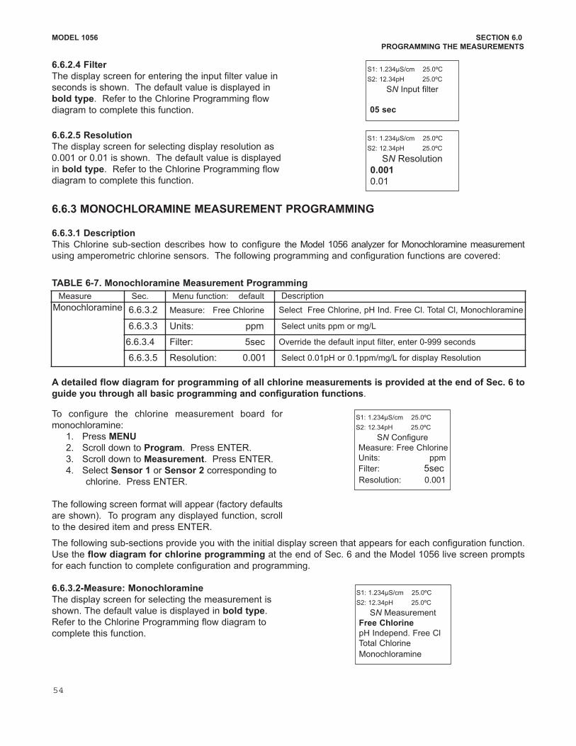
MODEL 1056 SECTION 6.0
PROGRAMMING THE MEASUREMENTS
6.6.2.4 Filter
The display screen for entering the input filter value in
seconds is shown. The default value is displayed in
bold type. Refer to the Chlorine Programming flow
diagram to complete this function.
S1: 1.234µS/cm 25.0ºC
S2: 12.34pH 25.0ºC
SN Input filter
05 sec
6.6.2.5 Resolution
The display screen for selecting display resolution as
0.001 or 0.01 is shown. The default value is displayed
in bold type. Refer to the Chlorine Programming flow
diagram to complete this function.
S1: 1.234µS/cm 25.0ºC
S2: 12.34pH 25.0ºC
SN Resolution
0.001
0.01
6.6.3 MONOCHLORAMINE MEASUREMENT PROGRAMMING
6.6.3.1 Description
This Chlorine subsection describes how to configure the Model 1056 analyzer for Monochloramine measurement
using amperometric chlorine sensors. The following programming and configuration functions are covered:
To configure the chlorine measurement board for
monochloramine:
1. Press MENU
2. Scroll down to Program. Press ENTER.
3. Scroll down to Measurement. Press ENTER.
4. Select Sensor 1 or Sensor 2 corresponding to
chlorine. Press ENTER.
The following screen format will appear (factory defaults
are shown). To program any displayed function, scroll
to the desired item and press ENTER.
Measure Sec. Menu function: default Description
Monochloramine 6.6.3.2 Measure: Free Chlorine Select Free Chlorine, pH Ind. Free Cl. Total Cl, Monochloramine
6.6.3.3 Units: ppm Select units ppm or mg/L
6.6.3.4 Filter: 5sec Override the default input filter, enter 0999 seconds
6.6.3.5 Resolution: 0.001 Select 0.01pH or 0.1ppm/mg/L for display Resolution
S1: 1.234µS/cm 25.0ºC
S2: 12.34pH 25.0ºC
SN Configure
Measure: Free Chlorine
Units: ppm
Filter: 5sec
Resolution: 0.001
The following subsections provide you with the initial display screen that appears for each configuration function.
Use the flow diagram for chlorine programming at the end of Sec. 6 and the Model 1056 live screen prompts
for each function to complete configuration and programming.
6.6.3.2Measure: Monochloramine
The display screen for selecting the measurement is
shown. The default value is displayed in bold type.
Refer to the Chlorine Programming flow diagram to
complete this function.
S1: 1.234µS/cm 25.0ºC
S2: 12.34pH 25.0ºC
SN Measurement
Free Chlorine
pH Independ. Free Cl
Total Chlorine
Monochloramine
TABLE 67. Monochloramine Measurement Programming
A detailed flow diagram for programming of all chlorine measurements is provided at the end of Sec. 6 to
guide you through all basic programming and configuration functions.
54
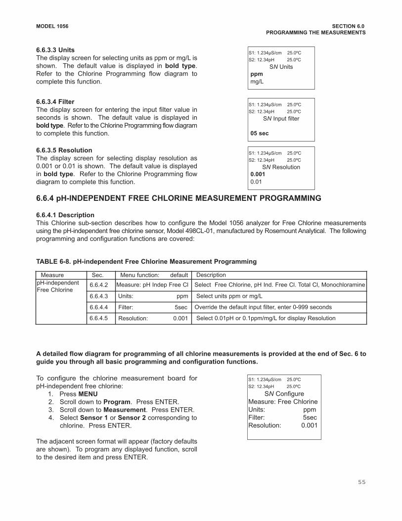
MODEL 1056 SECTION 6.0
PROGRAMMING THE MEASUREMENTS
6.6.4 pHINDEPENDENT FREE CHLORINE MEASUREMENT PROGRAMMING
6.6.4.1 Description
This Chlorine subsection describes how to configure the Model 1056 analyzer for Free Chlorine measurements
using the pHindependent free chlorine sensor, Model 498CL01, manufactured by Rosemount Analytical. The following
programming and configuration functions are covered:
To configure the chlorine measurement board for
pHindependent free chlorine:
1. Press MENU
2. Scroll down to Program. Press ENTER.
3. Scroll down to Measurement. Press ENTER.
4. Select Sensor 1 or Sensor 2 corresponding to
chlorine. Press ENTER.
The adjacent screen format will appear (factory defaults
are shown). To program any displayed function, scroll
to the desired item and press ENTER.
Measure Sec. Menu function: default Description
pHindependent
Free Chlorine6.6.4.2 Measure: pH Indep Free Cl Select Free Chlorine, pH Ind. Free Cl. Total Cl, Monochloramine
6.6.4.3 Units: ppm Select units ppm or mg/L
6.6.4.4 Filter: 5sec Override the default input filter, enter 0999 seconds
6.6.4.5 Resolution: 0.001 Select 0.01pH or 0.1ppm/mg/L for display Resolution
6.6.3.3 Units
The display screen for selecting units as ppm or mg/L is
shown. The default value is displayed in bold type.
Refer to the Chlorine Programming flow diagram to
complete this function.
S1: 1.234µS/cm 25.0ºC
S2: 12.34pH 25.0ºC
SN Units
ppm
mg/L
6.6.3.4 Filter
The display screen for entering the input filter value in
seconds is shown. The default value is displayed in
bold type. Refer to the Chlorine Programming flow diagram
to complete this function.
S1: 1.234µS/cm 25.0ºC
S2: 12.34pH 25.0ºC
SN Input filter
05 sec
6.6.3.5 Resolution
The display screen for selecting display resolution as
0.001 or 0.01 is shown. The default value is displayed
in bold type. Refer to the Chlorine Programming flow
diagram to complete this function.
S1: 1.234µS/cm 25.0ºC
S2: 12.34pH 25.0ºC
SN Resolution
0.001
0.01
S1: 1.234µS/cm 25.0ºC
S2: 12.34pH 25.0ºC
SN Configure
Measure: Free Chlorine
Units: ppm
Filter: 5sec
Resolution: 0.001
TABLE 68. pHindependent Free Chlorine Measurement Programming
A detailed flow diagram for programming of all chlorine measurements is provided at the end of Sec. 6 to
guide you through all basic programming and configuration functions.
55
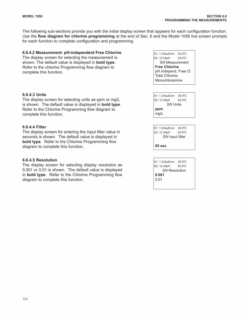
MODEL 1056 SECTION 6.0
PROGRAMMING THE MEASUREMENTS
6.6.4.2 Measurement: pHindependent Free Chlorine
The display screen for selecting the measurement is
shown. The default value is displayed in bold type.
Refer to the chlorine Programming flow diagram to
complete this function.
S1: 1.234µS/cm 25.0ºC
S2: 12.34pH 25.0ºC
SN Measurement
Free Chlorine
pH Independ. Free Cl
Total Chlorine
Monochloramine
6.6.4.3 Units
The display screen for selecting units as ppm or mg/L
is shown. The default value is displayed in bold type.
Refer to the Chlorine Programming flow diagram to
complete this function.
S1: 1.234µS/cm 25.0ºC
S2: 12.34pH 25.0ºC
SN Units
ppm
mg/L
6.6.4.4 Filter
The display screen for entering the input filter value in
seconds is shown. The default value is displayed in
bold type. Refer to the Chlorine Programming flow
diagram to complete this function.
S1: 1.234µS/cm 25.0ºC
S2: 12.34pH 25.0ºC
SN Input filter
05 sec
6.6.4.5 Resolution
The display screen for selecting display resolution as
0.001 or 0.01 is shown. The default value is displayed
in bold type. Refer to the Chlorine Programming flow
diagram to complete this function.
S1: 1.234µS/cm 25.0ºC
S2: 12.34pH 25.0ºC
SN Resolution
0.001
0.01
The following subsections provide you with the initial display screen that appears for each configuration function.
Use the flow diagram for chlorine programming at the end of Sec. 6 and the Model 1056 live screen prompts
for each function to complete configuration and programming.
56
6.7.3 Units
The display screen for selecting units as ppm , mg/L,
ppb, µg/L, % Saturation, %Oxygen in Gas, or ppm
Oxygen in Gas is shown. The default value is displayed
in bold type. Refer to the Oxygen Programming flow
diagram to complete this function.
MODEL 1056 SECTION 6.0
PROGRAMMING THE MEASUREMENTS
6.7.2 Oxygen Measurement application
The display screen for programming the measurement
is shown. The default value is displayed in bold type.
Refer to the Oxygen Programming flow diagram to
complete this function.
S1: 1.234µS/cm 25.0ºC
S2: 12.34pH 25.0ºC
SN Type
Water/Waste
Trace Oxygen
BioRxRosemount
BioRxOther
Brewing
Oxygen In Gas
6.7 OXYGEN MEASUREMENT PROGRAMMING6.7.1 Description
This section describes how to configure the Model 1056 analyzer for dissolved and gaseous oxygen measurement
using amperometric oxygen sensors. The following programming and configuration functions are covered:
To configure the Oxygen measurement board:
1. Press MENU
2. Scroll down to Program. Press ENTER.
3. Scroll down to Measurement. Press ENTER.
4. Select Sensor 1 or Sensor 2 corresponding to Oxygen.
Press ENTER.
The adjacent screen format will appear (factory defaults are
shown). To program any displayed function, scroll to the
desired item and press ENTER.
Measure Sec. Menu function: default Description
Oxygen 6.7.2 Type: Water/Waste Select Water/Waste, Trace. BioRx, BioRxOther, Brew, %O2 In Gas
6.7.3 Units: ppm Select ppm, mg/L, ppb, µg/L, % Sat, %O2Gas, ppm OxygenGas
6.7.4 Partial Press: mmHg Select mm Hg, in Hg. atm, kPa, mbar or bar for Partial pressure
6.7.5 Salinity: 00.0‰ Enter Salinity as ‰
6.7.6 Filter: 5sec Override the default input filter, enter 0999 seconds
6.7.7 Pressure Units: bar Select pressure units: mm Hg, in Hg,. Atm, kPa, mbar, bar
6.7.8 Use Press: At Air Cal Select atmospheric pressure source – internal or mA Input
S1: 1.234µS/cm 25.0ºC
S2: 12.34pH 25.0ºC
SN Configure
Type: Water/Waste
Units: ppm
Partial Press: mmHg
Salinity: 00.0‰
Filter: 5sec
Pressure Units: bar
Use Press: At Air Cal
Custom Setup
The following subsections show the initial display screen that appears for each configuration function. Use the
flow diagram for oxygen programming at the end of Sec. 6 and the Model 1056 live screen prompts for each
function to complete configuration and programming.
S1: 1.234µS/cm 25.0ºC
S2: 12.34pH 25.0ºC
SN Units
ppm
mg/L
ppb
µg/L
% Saturation
Partial Pressure
% Oxygen In Gas
ppm Oxygen In Gas
TABLE 69. Oxygen Measurement Programming
A detailed flow diagram for oxygen programming is provided at the end of Sec. 6 to guide you through all basic pro
gramming and configuration functions.
57
6.7.8 Use Pressure
The display screen for selecting atmospheric pressure
source. The default value is displayed in bold type.
Refer to the Oxygen Programming flow diagram to com
plete this function.
S1: 1.234µS/cm 25.0ºC
S2: 12.34pH 25.0ºC
SN Use Pressure?
At Air Cal
mA Input
MODEL 1056 SECTION 6.0
PROGRAMMING THE MEASUREMENTS
6.7.4 Partial Press
The display screen for selecting pressure units for
Partial pressure is shown. This selection is needed if
the specified measurement is Partial pressure. The
default value is displayed in bold type. Refer to the
Oxygen Programming flow diagram to complete this
function.
6.7.5 Salinity
The display screen for Entering the Salinity (as parts
per thousand) of the process liquid to be measured is
shown. The default value is displayed in bold type.
Refer to the Oxygen Programming flow diagram to
complete this function.
Enter Salinity as ‰
S1: 1.234µS/cm 25.0ºC
S2: 12.34pH 25.0ºC
SN Partial Press
mm Hg
in Hg
atm
kPa
mbar
bar
6.7.7 Pressure Units
The display screen for selecting pressure units for
atmospheric pressure is shown. This selection is needed
for the display of atmospheric pressure measured by
the onboard pressure transducer on the Oxygen
measurement board. The default value is displayed in
bold type. Refer to the Oxygen Programming flow
diagram to complete this function.
S1: 1.234µS/cm 25.0ºC
S2: 12.34pH 25.0ºC
Pressure Units
mm Hg
in Hg
atm
kPa
mbar
bar
S1: 1.234µS/cm 25.0ºC
S2: 12.34pH 25.0ºC
SN Salinity
00.0 ‰
6.7.6 Filter
The display screen for entering the input filter value in
seconds is shown. The default value is displayed in
bold type. Refer to the Oxygen Programming flow
diagram to complete this function.
S1: 1.234µS/cm 25.0ºC
S2: 12.34pH 25.0ºC
SN Input filter
05 sec
58
MODEL 1056 SECTION 6.0
PROGRAMMING THE MEASUREMENTS
6.8 OZONE MEASUREMENT PROGRAMMING
6.8.1 Description
This section describes how to configure the 1056 analyzer for ozone measurement using amperometric ozone sen
sors. The following programming and configuration functions are covered:
Measure Sec. Menu function: default Description
Ozone 6.8.2 Units: ppm Select units ppm, mg/L, ppb, µg/L
6.8.3 Filter: 5sec Override the default input filter, enter 0999 seconds
6.8.4 Resolution: 0.001 Select 0.01or 0.001 for display resolution
To configure the Ozone measurement board:
1. Press MENU
2. Scroll down to Program. Press ENTER.
3. Scroll down to Measurement. Press ENTER.
4. Select Sensor 1 or Sensor 2 corresponding to
Ozone. Press ENTER.
The adjacent screen format will appear (factory defaults
are shown). To program any displayed function, scroll to
the desired item and press ENTER.
S1: 1.234µS/cm 25.0ºC
S2: 12.34pH 25.0ºC
SN Configure
Units: ppm
Filter: 5 sec
Resolution: 0.001
6.8.2 Units
The display screen for selecting measurement units is
shown. The default value is displayed in bold type.
Refer to the Ozone Programming flow diagram to
complete this function.
S1: 1.234µS/cm 25.0ºC
S2: 12.34pH 25.0ºC
SN Units
ppm
mg/L
ppb
µg/L
6.8.3 Filter
The display screen for entering the input filter value in
seconds is shown. The default value is displayed in
bold type. Refer to the Ozone Programming flow
diagram to complete this function.
S1: 1.234µS/cm 25.0ºC
S2: 12.34pH 25.0ºC
SN Input filter
05 sec
6.8.4 Resolution
The display screen for selecting display resolution as
0.001 or 0.01 is shown. The default value is displayed
in bold type. Refer to the Ozone Programming flow
diagram to complete this function.
S1: 1.234µS/cm 25.0ºC
S2: 12.34pH 25.0ºC
SN Resolution
0.001
0.01
The following subsections show the initial display screen that appears for each configuration function. Use the
flow diagram for ozone programming at the end of Sec. 6 and the Model 1056 live screen prompts for each
function to complete configuration and programming.
Note: Ozone measurement boards are detected automatically by the analyzer. No measurement selection is necessary.
TABLE 610. Ozone Measurement Programming
A detailed flow diagram for ozone programming is provided at the end of Sec. 6 to guide you through all
basic programming and configuration functions.
59
MODEL 1056 SECTION 6.0
PROGRAMMING THE MEASUREMENTS
6.9 TURBIDITY MEASUREMENT PROGRAMMING
6.9.1 DESCRIPTION
This section describes how to configure the Model 1056 analyzer for Turbidity measurements. The following
programming and configuration functions are covered.
A detailed flow diagram for Turbidity programming is provided at the end of Sec. 6 to guide you through all basic
programming and configuration functions.
To configure the Turbidity measurement board:
1. Press MENU
2. Scroll down to Program. Press ENTER.
3. Scroll down to Measurement. Press ENTER.
4. Select Sensor 1 or Sensor 2 corresponding to Turbidity. Press ENTER.
The following screen format will appear (factory defaults are shown).
*TSS: Total Suspended Solids
6.9.2 Measurement
The display screen for selecting the measurement is
shown. The default measurement is displayed in bold
type. Refer to the Turbidity Programming flow diagram
to complete this function.
6.9.3 Units
The display screen for selecting the measurement
units is shown. The default value is displayed in bold
type. Refer to the Turbidity Programming flow diagram
to complete this function.
To program Turbidity, scroll to the desired item and press ENTER.
The following subsections provide you with the initial display screen that appears for each programming routine.
Use the flow diagram for Turbidity programming at the end of Sec. 6 and the live screen prompts to complete
programming.
S1: 1.234µS/cm 25.0ºC
S2: 12.34pH 25.0ºC
SN Configure
Measure: Turbidity
Units: NTU
Enter TSS Data
Filter: 20sec
Bubble Rejection: On
S1: 1.234µS/cm 25.0ºC
S2: 12.34pH 25.0ºC
SN Measurement
Turbidity
Calculated TSS
S1: 1.234µS/cm 25.0ºC
S2: 12.34pH 25.0ºC
SN Units
NTU
FTU
FNU
Measure Sec. Menu function: default Description
Turbidity 6.9.2 Measurement type: Turbidity Select Turbidity or TSS calculation (estimated TSS)
6.9.3 Measurement units: NTU NTU, FTU, FNU
6.9.4 Enter TSS* Data: Enter TSS and NTU data to calculate TSS based on Turbidity
6.9.5 Filter: 20 sec Override the default input filter, enter 0999 seconds
6.9.6 Bubble Rejection: OnIntelligent software algorithm to eliminate erroneous readings
caused by bubble accumulation in the sample
TABLE 611 TURBIDITY MEASUREMENT PROGRAMMING
60
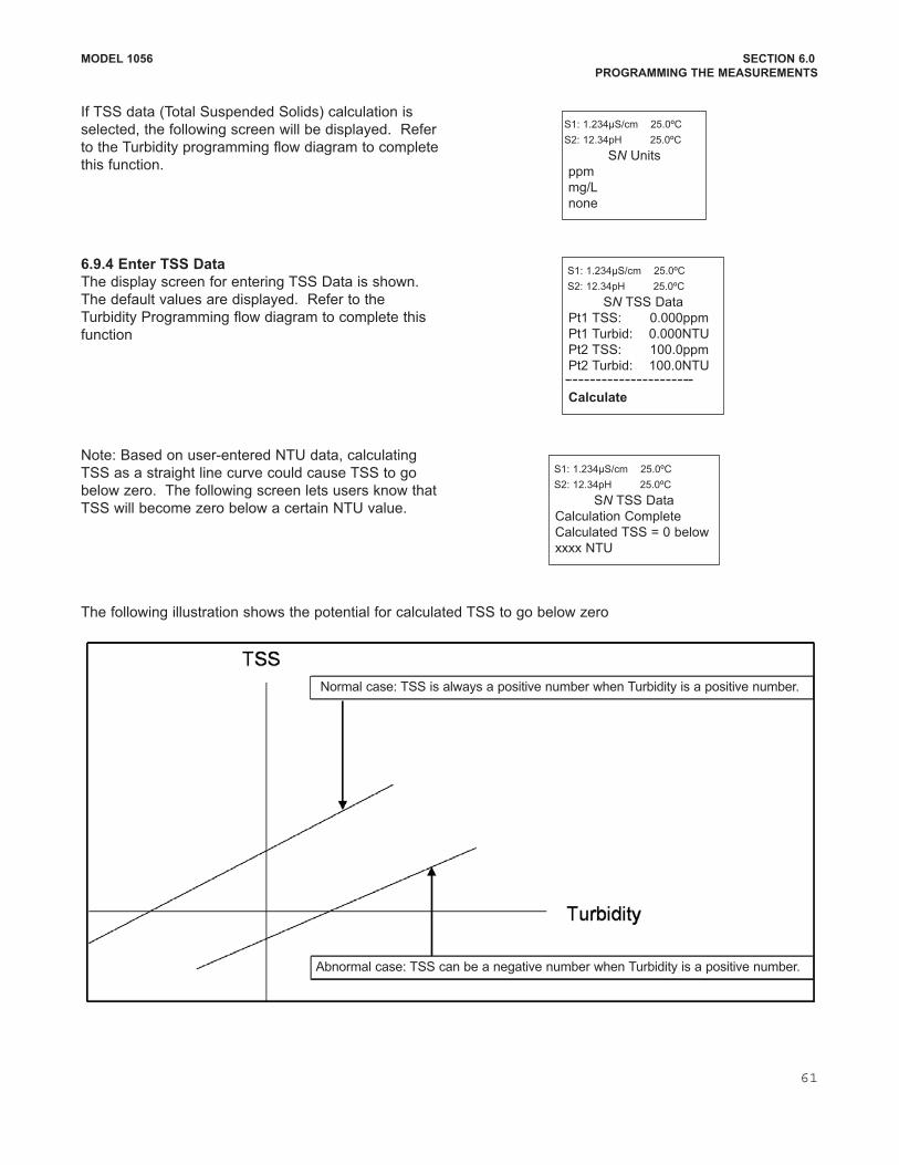
MODEL 1056 SECTION 6.0
PROGRAMMING THE MEASUREMENTS
If TSS data (Total Suspended Solids) calculation is
selected, the following screen will be displayed. Refer
to the Turbidity programming flow diagram to complete
this function.
6.9.4 Enter TSS Data
The display screen for entering TSS Data is shown.
The default values are displayed. Refer to the
Turbidity Programming flow diagram to complete this
function
Note: Based on userentered NTU data, calculating
TSS as a straight line curve could cause TSS to go
below zero. The following screen lets users know that
TSS will become zero below a certain NTU value.
The following illustration shows the potential for calculated TSS to go below zero
S1: 1.234µS/cm 25.0ºC
S2: 12.34pH 25.0ºC
SN Units
ppm
mg/L
none
S1: 1.234µS/cm 25.0ºC
S2: 12.34pH 25.0ºC
SN TSS Data
Calculation Complete
Calculated TSS = 0 below
xxxx NTU
S1: 1.234µS/cm 25.0ºC
S2: 12.34pH 25.0ºC
SN TSS Data
Pt1 TSS: 0.000ppm
Pt1 Turbid: 0.000NTU
Pt2 TSS: 100.0ppm
Pt2 Turbid: 100.0NTU
Calculate
61
Normal case: TSS is always a positive number when Turbidity is a positive number.
Abnormal case: TSS can be a negative number when Turbidity is a positive number.
MODEL 1056 SECTION 6.0
PROGRAMMING THE MEASUREMENTS
When the TSS data entry is complete, press ENTER.
The display will confirm the determination of a TSS
straight line curve fit to the entered NTU/turbidity data
by displaying this screen:
The following screen may appear if TSS calculation is
unsuccessful. Reentry of NTU and TSS data is
required.
6.9.5 Filter
The display screen for entering the input filter value in
seconds is shown. The default value is displayed in
bold type. Refer to the Turbidity Programming flow
diagram to complete this function.
6.9.6 Bubble Rejection
Bubble rejection is an internal software algorithm that
characterizes turbidity readings as bubbles as
opposed to true turbidity of the sample. With Bubble
rejection enabled, these erroneous readings are elimi
nated from the live measurements shown on the dis
play and transmitted via the current outputs.
The display screen for selecting bubble rejection algo
rithm is shown. The default setting is displayed in bold
type. Refer to the Turbidity Programming flow diagram
to complete this function.
S1: 1.234µS/cm 25.0ºC
S2: 12.34pH 25.0ºC
SN TSS Data
Calculation
Complete
S1: 1.234µS/cm 25.0ºC
S2: 12.34pH 25.0ºC
SN TSS Data
Data Entry Error
Press EXIT
S1: 1.234µS/cm 25.0ºC
S2: 12.34pH 25.0ºC
SN Input Filter
020sec
S1: 1.234µS/cm 25.0ºC
S2: 12.34pH 25.0ºC
SN Bubble Rejection
On
Off
62
MODEL 1056 SECTION 6.0
PROGRAMMING THE MEASUREMENTS
6.10.2 Measurement
The display screen for selecting the measurement is
shown. The default measurement is displayed in bold
type. Refer to the pulse flow Programming diagram to
complete this function.
6.10.4 Filter
The display screen for entering the input filter value in
seconds is shown. The default value is displayed in
bold type. Refer to the pulse flow Programming dia
gram to complete this function.
6.10.3 Units
The display screen for selecting measurement units is
shown. The default units are displayed in bold type.
Refer to the pulse flow Programming diagram to com
plete this function.
6.10 FLOW MEASUREMENT PROGRAMMING
6.10.1 DESCRIPTION
This section describes how to configure the 1056 analyzer for flow measurement when used with a compatible pulse
flow sensor. The following programming and configuration functions are covered.
To configure the flow measurement board:
1. Press MENU
2. Scroll down to Program. Press ENTER.
3. Scroll down to Measurement. Press ENTER.
4. Select Sensor 1 or Sensor 2 corresponding to
flow. Press ENTER.
The following screen format will appear (factory defaults
are shown).
To program pulse flow, scroll to the desired item and press ENTER.
The following subsections provide you with the initial display screen that appears for each programming routine.
Use the diagram for pulse flow programming at the end of Sec. 6 and the live screen prompts to complete
programming.
S1: 1.234µS/cm 25.0ºC
S2: 12.34pH 25.0ºC
SN Configure
Measure: Pulse Flow
Units: GPM
Filter: 5sec
S1: 1.234µS/cm 25.0ºC
S2: 12.34pH 25.0ºC
SN Measurement
Pulse Flow
mA Input
S1: 1.234µS/cm 25.0ºC
S2: 12.34pH 25.0ºC
SN Input Filter
005sec
S1: 1.234µS/cm 25.0ºC
S2: 12.34pH 25.0ºC
SN Units
GPM
GPH
cu ft/min
cu ft/hour
L/min
L/hour
m3/hour
Measure Sec. Menu function: default Description
Flow 6.10.2 Measurement type Pulse Flow Select Pulse Flow or mA Current Input
6.10.3 Measurement units: GPH Select GPM, GPH, cu ft/min, cu ft/hour, LPM, L/hour, m3/hr
6.10.4 Enter TSS* Data: 0 Sec Override the default input filter, enter 0999 seconds
TABLE 612 FLOW MEASUREMENT PROGRAMMING
63
To configure the current input measurement board:
1. Press MENU
2. Scroll down to Program. Press ENTER.
3. Scroll down to Measurement. Press ENTER.
4. Select Sensor 1 or Sensor 2 corresponding to
current input. Press ENTER.
Note that factory default is Pulse Flow not mA Input.
The user must override the factory default and select
mA Input to enable the current input functionality. Upon
selecting mA Input, the following menu screen will
appear to allow complete programming of mA Current
Input.
MODEL 1056 SECTION 6.0
PROGRAMMING THE MEASUREMENTS
6.11 CURRENT INPUT PROGRAMMING
6.11.1 DESCRIPTION
This section describes how to configure the Model 1056 analyzer for current input measurement when wired to an
external device that transmits 420mA or 020mA analog current output. The following programming and configu
ration functions are covered.
6.11.2 Measurement
The display screen for selecting the signal board func
tionality is shown. The default value is displayed in
bold type. Scroll down to select mA Input to enable
the current input functionality. Refer to the current
input Programming flow diagram to complete this func
tion.
6.11.3 mA Input
The display screen for selecting the type of measure
ment is shown. The default measurement type for mA
Input is displayed in bold type. Refer to the current
input Programming flow diagram to complete this function.
To program current input, scroll to the desired item and press ENTER.
The following subsections provide you with the initial display screen that appears for each programming routine.
Use the flow diagram for current input programming at the end of Sec. 6 and the live screen prompts to complete
programming.
A detailed flow diagram for current input programming is provided at the end of Sec. 6 to guide you through all
basic programming and configuration functions.
S1: 1.234µS/cm 25.0ºC
S2: 12.34pH 25.0ºC
SN Configure
Measure: mA Input
mA Input: Temperature
Units: ºC
Input Range: 420mA
Low Value: 0.001%
High Value : 100.0%
Filter: 5sec
S1: 1.234µS/cm 25.0ºC
S2: 12.34pH 25.0ºC
SN Measurement
Pulse Flow
mA Input
S1: 1.234µS/cm 25.0ºC
S2: 12.34pH 25.0ºC
SN mA Input
Temperature
Pressure
Flow
Other
Measure Sec. Menu function: default Description
Current
Input6.11.2 Measurement type mA input Override the default (Flow) and select mA current input
6.11.3 mA Input Temperature Select Temperature, Pressure, Flow or Other
6.11.4 Measurement units: ºC Select measurement units based on selected input device type
6.11.5 Input Range: 420mA Select 420mA or 020mA
6.11.6 Low Value: 0.000ºC Enter the low measurement value to assign to 4mA
6.11.7 High Value: 100.0ºC Enter the high measurement value to assign to 20mA
6.11.8 Filter: 05 sec Override the default input filter, enter 0999 seconds
TABLE 613 CURRENT INPUT PROGRAMMING
64
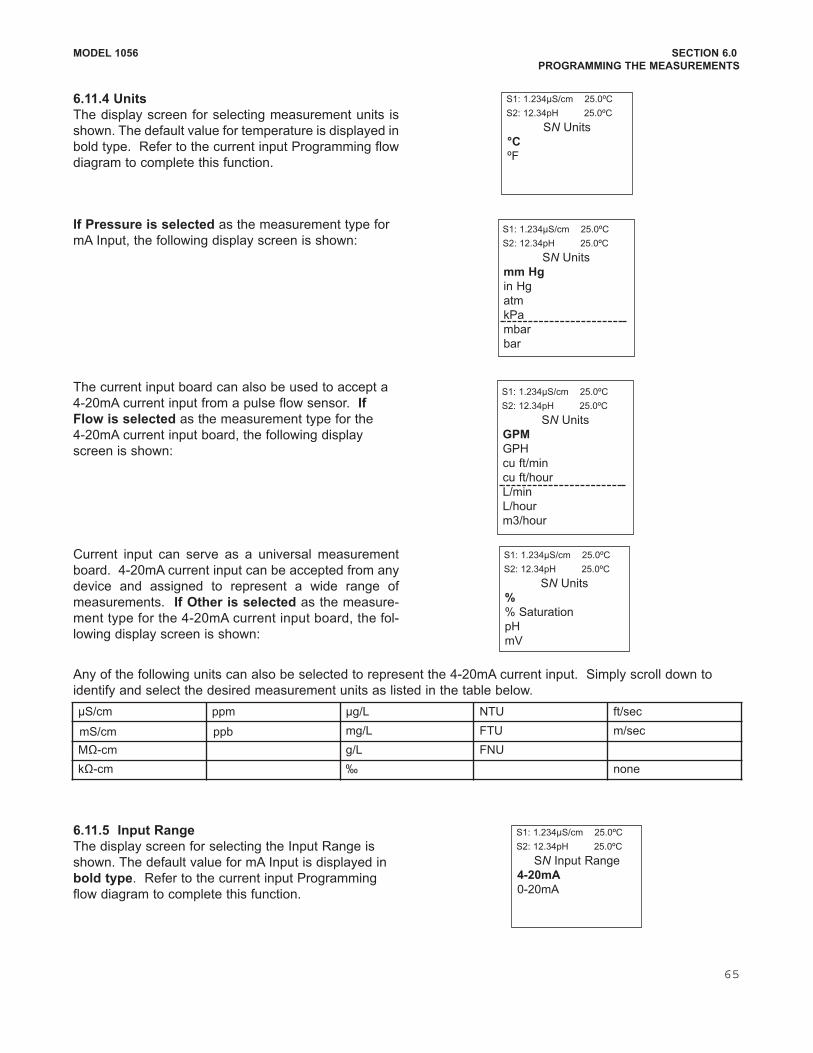
MODEL 1056 SECTION 6.0
PROGRAMMING THE MEASUREMENTS
6.11.4 Units
The display screen for selecting measurement units is
shown. The default value for temperature is displayed in
bold type. Refer to the current input Programming flow
diagram to complete this function.
If Pressure is selected as the measurement type for
mA Input, the following display screen is shown:
Current input can serve as a universal measurement
board. 420mA current input can be accepted from any
device and assigned to represent a wide range of
measurements. If Other is selected as the measure
ment type for the 420mA current input board, the fol
lowing display screen is shown:
6.11.5 Input Range
The display screen for selecting the Input Range is
shown. The default value for mA Input is displayed in
bold type. Refer to the current input Programming
flow diagram to complete this function.
The current input board can also be used to accept a
420mA current input from a pulse flow sensor. If
Flow is selected as the measurement type for the
420mA current input board, the following display
screen is shown:
Any of the following units can also be selected to represent the 420mA current input. Simply scroll down to
identify and select the desired measurement units as listed in the table below.
S1: 1.234µS/cm 25.0ºC
S2: 12.34pH 25.0ºC
SN Units
°C
ºF
S1: 1.234µS/cm 25.0ºC
S2: 12.34pH 25.0ºC
SN Units
%
% Saturation
pH
mV
S1: 1.234µS/cm 25.0ºC
S2: 12.34pH 25.0ºC
SN Input Range
420mA
020mA
S1: 1.234µS/cm 25.0ºC
S2: 12.34pH 25.0ºC
SN Units
mm Hg
in Hg
atm
kPa
mbar
bar
S1: 1.234µS/cm 25.0ºC
S2: 12.34pH 25.0ºC
SN Units
GPM
GPH
cu ft/min
cu ft/hour
L/min
L/hour
m3/hour
µS/cm ppm µg/L NTU ft/sec
mS/cm ppb mg/L FTU m/sec
MΩcm g/L FNU
kΩcm ‰ none
65

6.11.6 Low Value
The display screen for entering the Low Value to be
assigned to 4mA (or 0mA) current input is shown. The
default value for temperature is displayed in bold type.
Refer to the current input Programming flow diagram
to complete this function.
6.11.7 High Value
The display screen for entering the High Value to be
assigned to 20mA current input is shown. The default
value for temperature is displayed in bold type. Refer
to the current input Programming flow diagram to com
plete this function.
6.11.8 Filter
The display screen for entering the input filter value in
seconds is shown. The default value is displayed in
bold type. Refer to the current input Programming
diagram to complete this function. .
MODEL 1056 SECTION 6.0
PROGRAMMING THE MEASUREMENTS
S1: 1.234µS/cm 25.0ºC
S2: 12.34pH 25.0ºC
SN Low Value
0.000ºC
S1: 1.234µS/cm 25.0ºC
S2: 12.34pH 25.0ºC
SN High Value
100.0ºC
S1: 1.234µS/cm 25.0ºC
S2: 12.34pH 25.0ºC
SN Input Filter
005sec
66
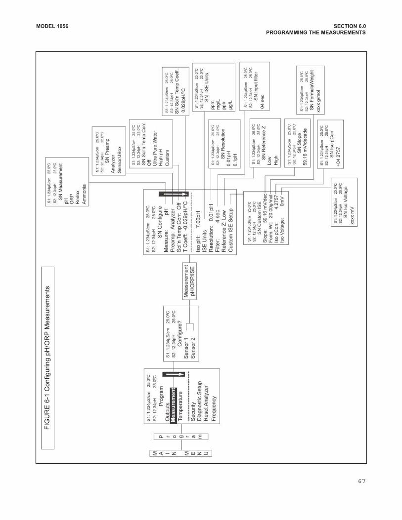
MODEL 1056 SECTION 6.0
PROGRAMMING THE MEASUREMENTS
FIG
UR
E 6
1 C
onfiguring p
H/O
RP
Measure
ments
67
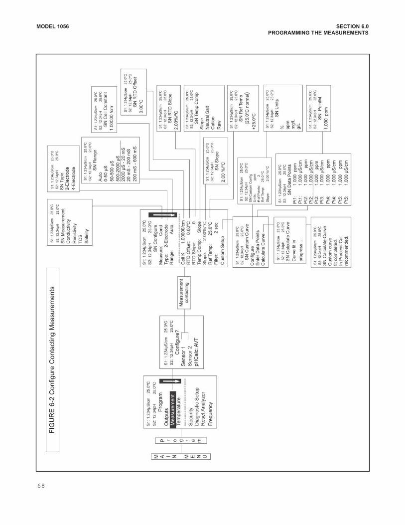
MODEL 1056 SECTION 6.0
PROGRAMMING THE MEASUREMENTS
FIG
UR
E 6
2 C
onfigure
Con
tacting M
easure
ments
68
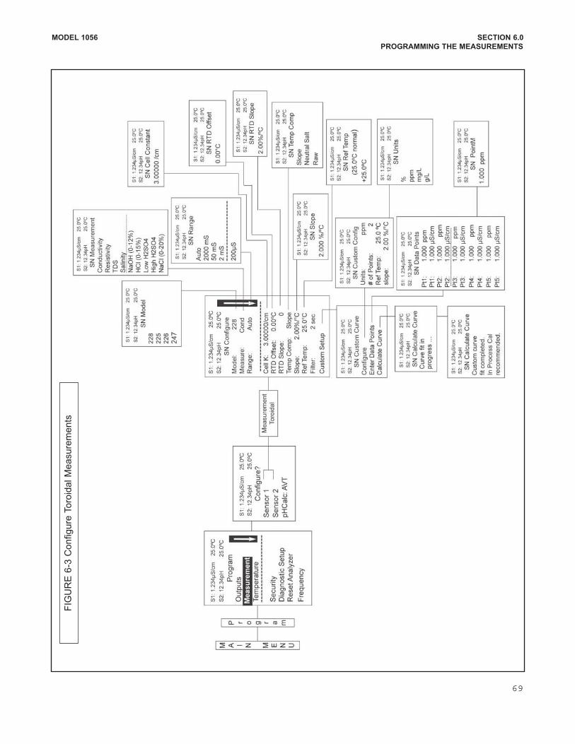
MODEL 1056 SECTION 6.0
PROGRAMMING THE MEASUREMENTS
FIG
UR
E 6
3 C
onfigure
To
roid
al M
easure
ments
69
MODEL 1056 SECTION 6.0
PROGRAMMING THE MEASUREMENTS
FIG
UR
E 6
5 C
on
figure
Oxygen M
easure
ments
70
MODEL 1056 SECTION 6.0
PROGRAMMING THE MEASUREMENTS
FIGURE 66 Configure Ozone Measurements
FIGURE 64 Configure Chlorine Measurements
71
MODEL 1056 SECTION 6.0
PROGRAMMING THE MEASUREMENTS
FIG
UR
E 6
7 C
onfigure
Turb
idity M
easure
ment
72
MODEL 1056 SECTION 6.0
PROGRAMMING THE MEASUREMENTS
FIGURE 68 Configure Flow Measurement
FIGURE 69 Configure mA Current Input Measurement
73

This page left blank intentionally
MODEL 1056 SECTION 6.0
PROGRAMMING THE MEASUREMENTS
74
MODEL 1056 SECTION 7.0
CALIBRATION
SECTION 7.0
CALIBRATION
7.1 CALIBRATION – INTRODUCTION
7.2 pH CALIBRATION
7.3 ORP CALIBRATION
7.4 CONTACTING CONDUCTIVITY CALIBRATION
7.5 TOROIDAL CONDUCTIVITY CALIBRATION
7.6 CHLORINE CALIBRATION
7.6.1 FREE CHLORINE
7.6.2 TOTAL CHLORINE
7.6.3 MONOCHLORAMINE
7.6.4 pHINDEPENDENT FREE CHLORINE
7.7 OXYGEN CALIBRATION
7.8 OZONE CALIBRATION
7.9 TEMPERATURE CALIBRATION
7.10 TURBIDITY CALIBRATION
7.11 FLOW CALIBRATION
7.1 CALIBRATION – INTRODUCTIONCalibration is the process of adjusting or standardizingthe analyzer to a lab test or a calibrated laboratoryinstrument, or standardizing to some known reference(such as a commercial buffer).
The autorecognition feature of the analyzer will enablethe appropriate calibration screens to allow calibration forany single sensor configuration or dual sensor configuration of the analyzer. Completion of Quick Start uponfirst power up enables live measurements but does notensure accurate readings in the lab or in process.Calibration should be performed with each attachedsensor to ensure accurate, repeatable readings.
This section covers the following programming andconfiguration functions:
1. Auto buffer cal for pH (pH Cal Sec.7.2)2. Manual buffer cal for pH (pH Cal Sec.7.2)3. Set calibration stabilization criteria for pH (pH Cal
Sec.7.2)
4. Standardization calibration (1point) for pH, ORP and Redox (pH Cal Sec.7.2 and 7.3)
5. Entering the cell constant of a conductivitysensor (Conductivity Cal Sec. 7.4 and 7.5)
6. Calibrating the sensor in a conductivity standard Conductivity Cal Sec. 7.4 and 7.5)
7. Calibrating the analyzer to a laboratory instrument (Contacting Conductivity Cal Sec.7.4)
8. Zeroing an chlorine, oxygen or ozone sensor (Amperometric Cal Sec’s 7.6, 7.7, 7.8)
9. Calibrating an oxygen sensor in air (Oxygen Cal Sec’s 7.6)
10. Calibrating the sensor to a sample of knownconcentration (Amperometric Cal Sec’s 7.6, 7.7, 7.8)
11. Enter a manual reference temperature fortemperature compensation of the process measurement
75
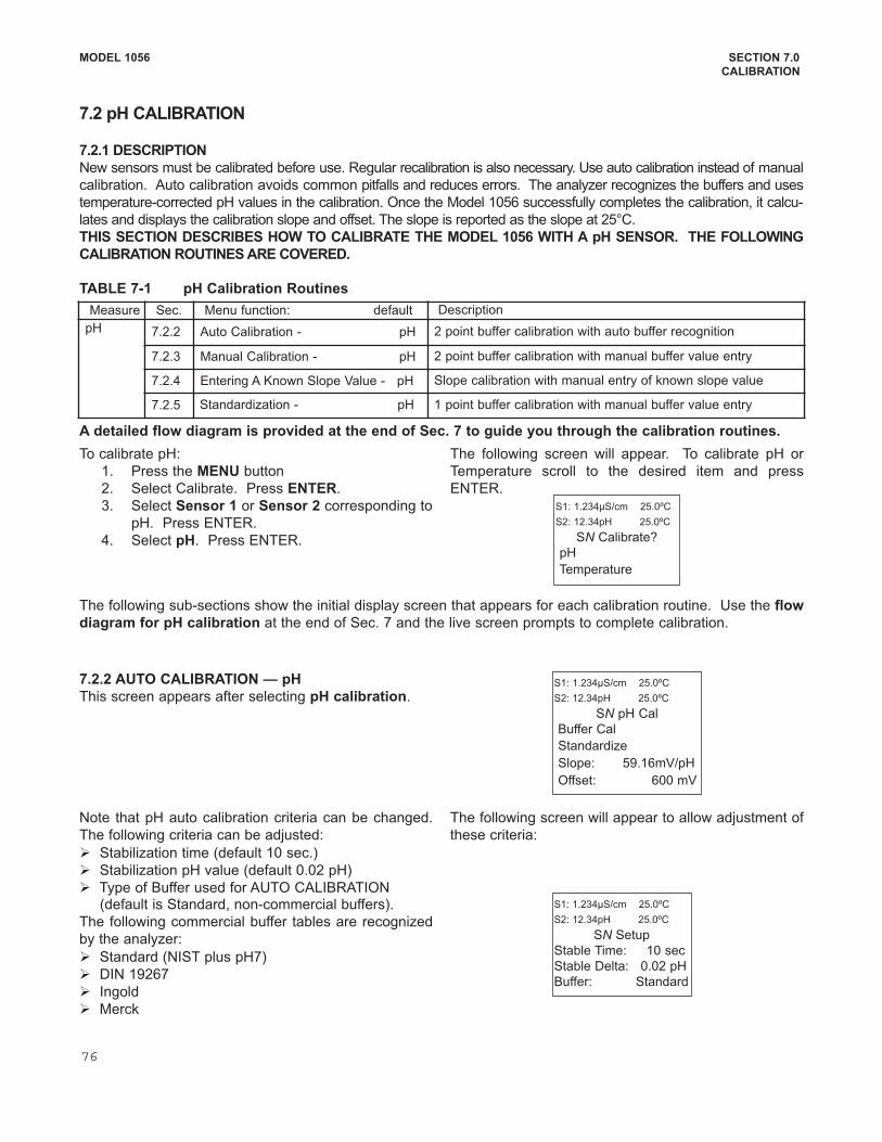
MODEL 1056 SECTION 7.0
CALIBRATION
7.2 pH CALIBRATION
7.2.1 DESCRIPTION
New sensors must be calibrated before use. Regular recalibration is also necessary. Use auto calibration instead of manual
calibration. Auto calibration avoids common pitfalls and reduces errors. The analyzer recognizes the buffers and uses
temperaturecorrected pH values in the calibration. Once the Model 1056 successfully completes the calibration, it calcu
lates and displays the calibration slope and offset. The slope is reported as the slope at 25°C.
THIS SECTION DESCRIBES HOW TO CALIBRATE THE MODEL 1056 WITH A pH SENSOR. THE FOLLOWING
CALIBRATION ROUTINES ARE COVERED.
Measure Sec. Menu function: default Description
pH 7.2.2 Auto Calibration pH 2 point buffer calibration with auto buffer recognition
7.2.3 Manual Calibration pH 2 point buffer calibration with manual buffer value entry
7.2.4 Entering A Known Slope Value pH Slope calibration with manual entry of known slope value
7.2.5 Standardization pH 1 point buffer calibration with manual buffer value entry
A detailed flow diagram is provided at the end of Sec. 7 to guide you through the calibration routines.
TABLE 71 pH Calibration Routines
To calibrate pH:
1. Press the MENU button
2. Select Calibrate. Press ENTER.
3. Select Sensor 1 or Sensor 2 corresponding to
pH. Press ENTER.
4. Select pH. Press ENTER.
The following screen will appear. To calibrate pH or
Temperature scroll to the desired item and press
ENTER. S1: 1.234µS/cm 25.0ºC
S2: 12.34pH 25.0ºC
SN Calibrate?
pH
Temperature
7.2.2 AUTO CALIBRATION — pH
This screen appears after selecting pH calibration.
Note that pH auto calibration criteria can be changed.
The following criteria can be adjusted:
Stabilization time (default 10 sec.)
Stabilization pH value (default 0.02 pH)
Type of Buffer used for AUTO CALIBRATION (default is Standard, noncommercial buffers).
The following commercial buffer tables are recognized
by the analyzer:
Standard (NIST plus pH7)
DIN 19267
Ingold
Merck
The following screen will appear to allow adjustment of
these criteria:
S1: 1.234µS/cm 25.0ºC
S2: 12.34pH 25.0ºC
SN pH Cal
Buffer Cal
Standardize
Slope: 59.16mV/pH
Offset: 600 mV
S1: 1.234µS/cm 25.0ºC
S2: 12.34pH 25.0ºC
SN Setup
Stable Time: 10 sec
Stable Delta: 0.02 pH
Buffer: Standard
The following subsections show the initial display screen that appears for each calibration routine. Use the flow
diagram for pH calibration at the end of Sec. 7 and the live screen prompts to complete calibration.
76
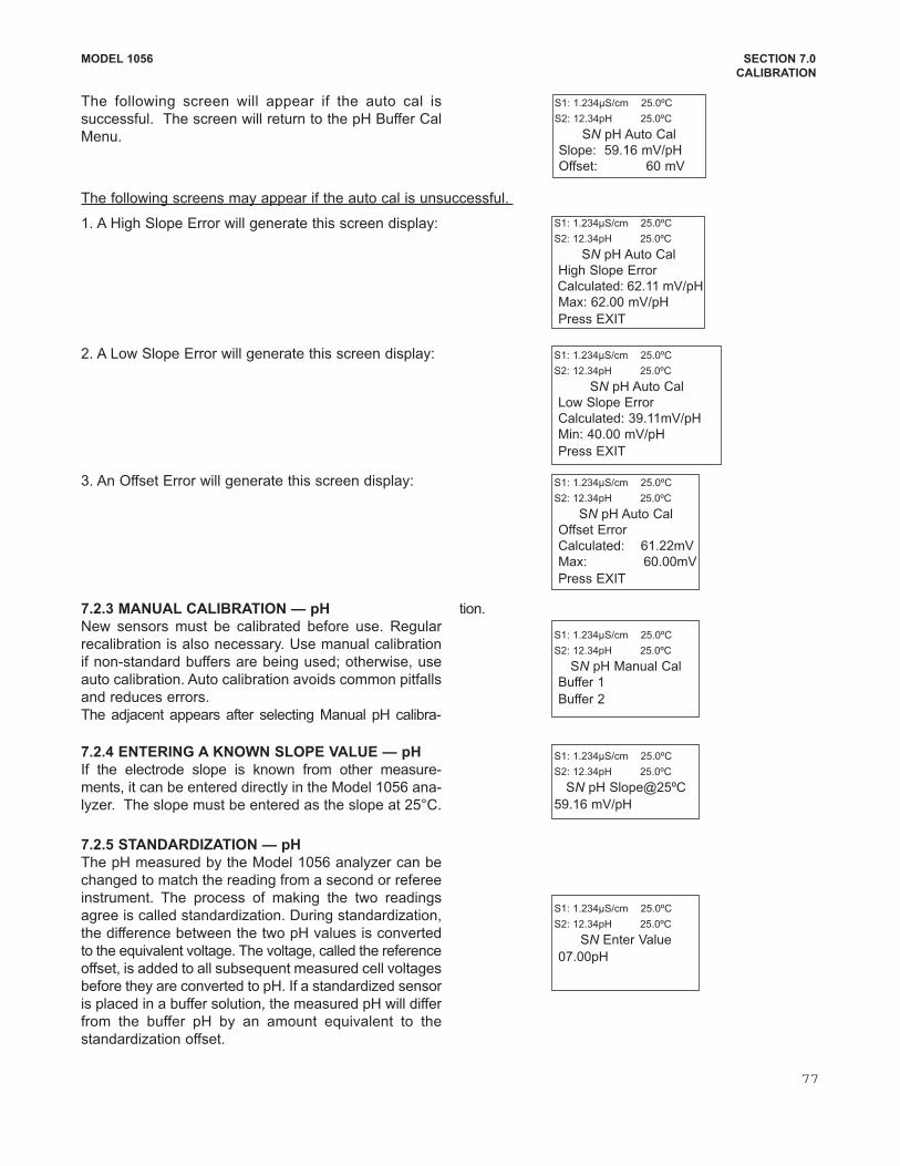
MODEL 1056 SECTION 7.0
CALIBRATION
The following screen will appear if the auto cal is
successful. The screen will return to the pH Buffer Cal
Menu.
S1: 1.234µS/cm 25.0ºC
S2: 12.34pH 25.0ºC
SN pH Auto Cal
Slope: 59.16 mV/pH
Offset: 60 mV
1. A High Slope Error will generate this screen display:
2. A Low Slope Error will generate this screen display:
S1: 1.234µS/cm 25.0ºC
S2: 12.34pH 25.0ºC
SN pH Auto Cal
High Slope Error
Calculated: 62.11 mV/pH
Max: 62.00 mV/pH
Press EXIT
3. An Offset Error will generate this screen display:
S1: 1.234µS/cm 25.0ºC
S2: 12.34pH 25.0ºC
SN pH Auto Cal
Low Slope Error
Calculated: 39.11mV/pH
Min: 40.00 mV/pH
Press EXIT
S1: 1.234µS/cm 25.0ºC
S2: 12.34pH 25.0ºC
SN pH Auto Cal
Offset Error
Calculated: 61.22mV
Max: 60.00mV
Press EXIT
7.2.3 MANUAL CALIBRATION — pH
New sensors must be calibrated before use. Regular
recalibration is also necessary. Use manual calibration
if nonstandard buffers are being used; otherwise, use
auto calibration. Auto calibration avoids common pitfalls
and reduces errors.
The adjacent appears after selecting Manual pH calibra
tion.
S1: 1.234µS/cm 25.0ºC
S2: 12.34pH 25.0ºC
SN pH Manual Cal
Buffer 1
Buffer 2
7.2.5 STANDARDIZATION — pH
The pH measured by the Model 1056 analyzer can be
changed to match the reading from a second or referee
instrument. The process of making the two readings
agree is called standardization. During standardization,
the difference between the two pH values is converted
to the equivalent voltage. The voltage, called the reference
offset, is added to all subsequent measured cell voltages
before they are converted to pH. If a standardized sensor
is placed in a buffer solution, the measured pH will differ
from the buffer pH by an amount equivalent to the
standardization offset.
S1: 1.234µS/cm 25.0ºC
S2: 12.34pH 25.0ºC
SN Enter Value
07.00pH
7.2.4 ENTERING A KNOWN SLOPE VALUE — pH
If the electrode slope is known from other measure
ments, it can be entered directly in the Model 1056 ana
lyzer. The slope must be entered as the slope at 25°C.
S1: 1.234µS/cm 25.0ºC
S2: 12.34pH 25.0ºC
SN pH Slope@25ºC
59.16 mV/pH
The following screens may appear if the auto cal is unsuccessful.
77
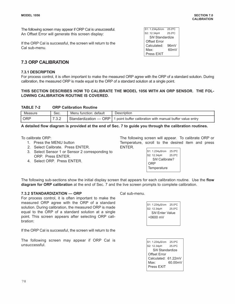
MODEL 1056 SECTION 7.0
CALIBRATION
7.3 ORP CALIBRATION
7.3.1 DESCRIPTION
For process control, it is often important to make the measured ORP agree with the ORP of a standard solution. During
calibration, the measured ORP is made equal to the ORP of a standard solution at a single point.
Measure Sec. Menu function: default Description
ORP 7.3.2 Standardization — ORP 1 point buffer calibration with manual buffer value entry
To calibrate ORP:
1. Press the MENU button
2. Select Calibrate. Press ENTER.
3. Select Sensor 1 or Sensor 2 corresponding to
ORP. Press ENTER.
4. Select ORP. Press ENTER.
The following screen will appear. To calibrate ORP or
Temperature, scroll to the desired item and press
ENTER. S1: 1.234µS/cm 25.0ºC
S2: 12.34pH 25.0ºC
SN Calibrate?
ORP
Temperature
7.3.2 STANDARDIZATION — ORP
For process control, it is often important to make the
measured ORP agree with the ORP of a standard
solution. During calibration, the measured ORP is made
equal to the ORP of a standard solution at a single
point. This screen appears after selecting ORP cali
bration:
If the ORP Cal is successful, the screen will return to the
Cal submenu.
The following screen may appear if ORP Cal is
unsuccessful.
S1: 1.234µS/cm 25.0ºC
S2: 12.34pH 25.0ºC
SN Enter Value
+0600 mV
S1: 1.234µS/cm 25.0ºC
S2: 12.34pH 25.0ºC
SN Standardize
Offset Error
Calculated: 61.22mV
Max: 60.00mV
Press EXIT
THIS SECTION DESCRIBES HOW TO CALIBRATE THE MODEL 1056 WITH AN ORP SENSOR. THE FOL
LOWING CALIBRATION ROUTINE IS COVERED.
A detailed flow diagram is provided at the end of Sec. 7 to guide you through the calibration routines.
The following subsections show the initial display screen that appears for each calibration routine. Use the flow
diagram for ORP calibration at the end of Sec. 7 and the live screen prompts to complete calibration.
TABLE 72 ORP Calibration Routine
The following screen may appear if ORP Cal is unsuccessful.
An Offset Error will generate this screen display:
If the ORP Cal is successful, the screen will return to the
Cal submenu.
S1: 1.234µS/cm 25.0ºC
S2: 12.34pH 25.0ºC
SN Standardize
Offset Error
Calculated: 96mV
Max: 60mV
Press EXIT
78
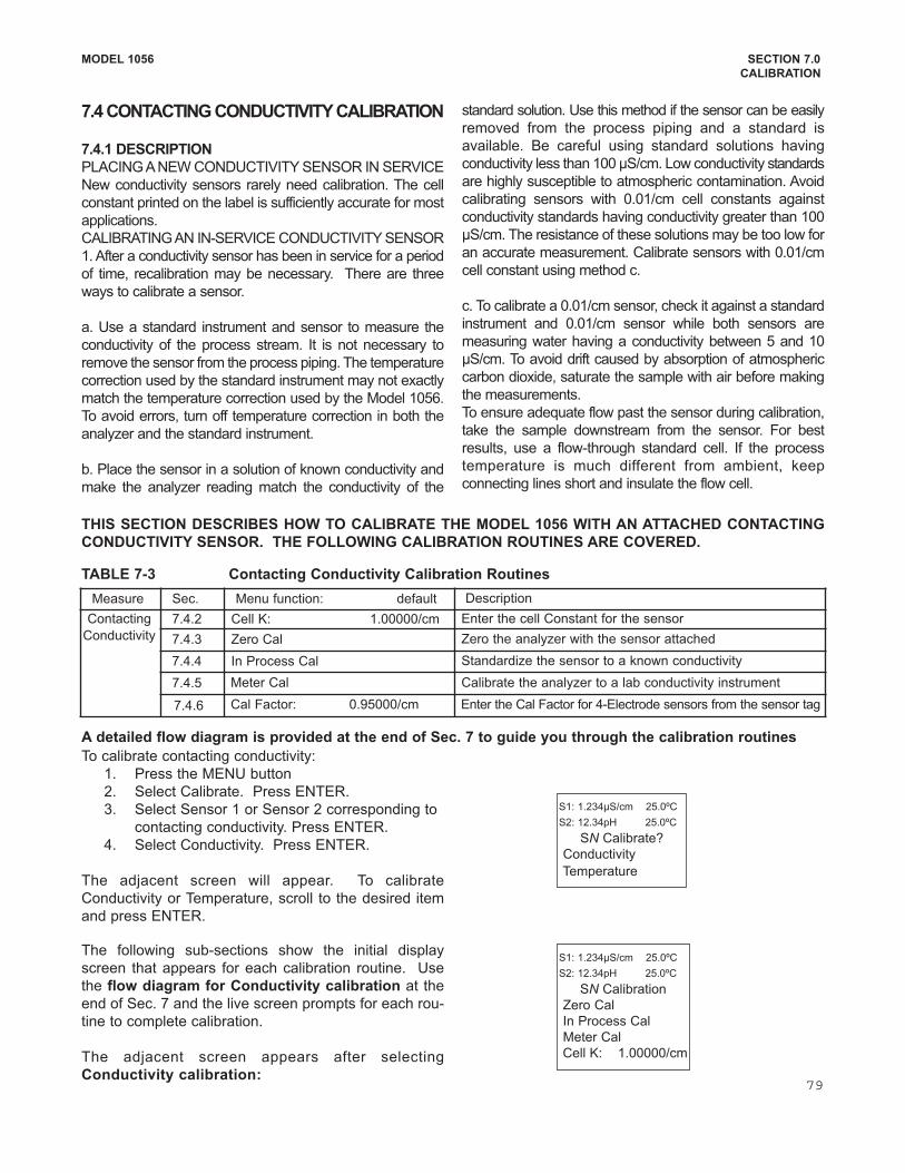
The following subsections show the initial display
screen that appears for each calibration routine. Use
the flow diagram for Conductivity calibration at the
end of Sec. 7 and the live screen prompts for each rou
tine to complete calibration.
The adjacent screen appears after selecting
Conductivity calibration:
MODEL 1056 SECTION 7.0
CALIBRATION
To calibrate contacting conductivity:
1. Press the MENU button
2. Select Calibrate. Press ENTER.
3. Select Sensor 1 or Sensor 2 corresponding to
contacting conductivity. Press ENTER.
4. Select Conductivity. Press ENTER.
The adjacent screen will appear. To calibrate
Conductivity or Temperature, scroll to the desired item
and press ENTER.
S1: 1.234µS/cm 25.0ºC
S2: 12.34pH 25.0ºC
SN Calibrate?
Conductivity
Temperature
S1: 1.234µS/cm 25.0ºC
S2: 12.34pH 25.0ºC
SN Calibration
Zero Cal
In Process Cal
Meter Cal
Cell K: 1.00000/cm
7.4 CONTACTING CONDUCTIVITY CALIBRATION
7.4.1 DESCRIPTION
PLACING A NEW CONDUCTIVITY SENSOR IN SERVICE
New conductivity sensors rarely need calibration. The cell
constant printed on the label is sufficiently accurate for most
applications.
CALIBRATING AN INSERVICE CONDUCTIVITY SENSOR
1. After a conductivity sensor has been in service for a period
of time, recalibration may be necessary. There are three
ways to calibrate a sensor.
a. Use a standard instrument and sensor to measure the
conductivity of the process stream. It is not necessary to
remove the sensor from the process piping. The temperature
correction used by the standard instrument may not exactly
match the temperature correction used by the Model 1056.
To avoid errors, turn off temperature correction in both the
analyzer and the standard instrument.
b. Place the sensor in a solution of known conductivity and
make the analyzer reading match the conductivity of the
standard solution. Use this method if the sensor can be easily
removed from the process piping and a standard is
available. Be careful using standard solutions having
conductivity less than 100 µS/cm. Low conductivity standards
are highly susceptible to atmospheric contamination. Avoid
calibrating sensors with 0.01/cm cell constants against
conductivity standards having conductivity greater than 100
µS/cm. The resistance of these solutions may be too low for
an accurate measurement. Calibrate sensors with 0.01/cm
cell constant using method c.
c. To calibrate a 0.01/cm sensor, check it against a standard
instrument and 0.01/cm sensor while both sensors are
measuring water having a conductivity between 5 and 10
µS/cm. To avoid drift caused by absorption of atmospheric
carbon dioxide, saturate the sample with air before making
the measurements.
To ensure adequate flow past the sensor during calibration,
take the sample downstream from the sensor. For best
results, use a flowthrough standard cell. If the process
temperature is much different from ambient, keep
connecting lines short and insulate the flow cell.
THIS SECTION DESCRIBES HOW TO CALIBRATE THE MODEL 1056 WITH AN ATTACHED CONTACTING
CONDUCTIVITY SENSOR. THE FOLLOWING CALIBRATION ROUTINES ARE COVERED.
A detailed flow diagram is provided at the end of Sec. 7 to guide you through the calibration routines
Measure Sec. Menu function: default Description
Contacting
Conductivity
7.4.2 Cell K: 1.00000/cm Enter the cell Constant for the sensor
7.4.3 Zero Cal Zero the analyzer with the sensor attached
7.4.4 In Process Cal Standardize the sensor to a known conductivity
7.4.5 Meter Cal Calibrate the analyzer to a lab conductivity instrument
7.4.6 Cal Factor: 0.95000/cm Enter the Cal Factor for 4Electrode sensors from the sensor tag
TABLE 73 Contacting Conductivity Calibration Routines
79
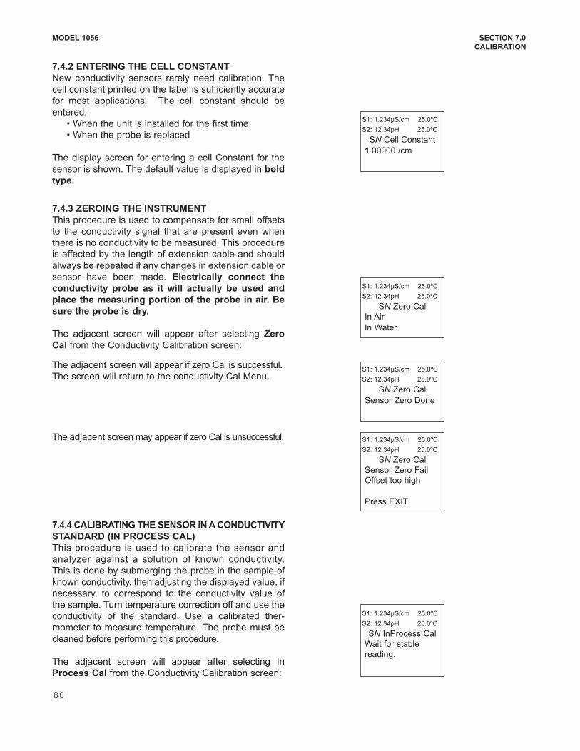
MODEL 1056 SECTION 7.0
CALIBRATION
7.4.2 ENTERING THE CELL CONSTANT
New conductivity sensors rarely need calibration. The
cell constant printed on the label is sufficiently accurate
for most applications. The cell constant should be
entered:
• When the unit is installed for the first time
• When the probe is replaced
The display screen for entering a cell Constant for the
sensor is shown. The default value is displayed in bold
type.
7.4.3 ZEROING THE INSTRUMENT
This procedure is used to compensate for small offsets
to the conductivity signal that are present even when
there is no conductivity to be measured. This procedure
is affected by the length of extension cable and should
always be repeated if any changes in extension cable or
sensor have been made. Electrically connect the
conductivity probe as it will actually be used and
place the measuring portion of the probe in air. Be
sure the probe is dry.
The adjacent screen will appear after selecting Zero
Cal from the Conductivity Calibration screen:
The adjacent screen will appear if zero Cal is successful.
The screen will return to the conductivity Cal Menu.
The adjacent screen may appear if zero Cal is unsuccessful.
S1: 1.234µS/cm 25.0ºC
S2: 12.34pH 25.0ºC
SN Cell Constant
1.00000 /cm
S1: 1.234µS/cm 25.0ºC
S2: 12.34pH 25.0ºC
SN Zero Cal
In Air
In Water
7.4.4 CALIBRATING THE SENSOR IN A CONDUCTIVITY
STANDARD (IN PROCESS CAL)
This procedure is used to calibrate the sensor and
analyzer against a solution of known conductivity.
This is done by submerging the probe in the sample of
known conductivity, then adjusting the displayed value, if
necessary, to correspond to the conductivity value of
the sample. Turn temperature correction off and use the
conductivity of the standard. Use a calibrated ther
mometer to measure temperature. The probe must be
cleaned before performing this procedure.
The adjacent screen will appear after selecting In
Process Cal from the Conductivity Calibration screen:
S1: 1.234µS/cm 25.0ºC
S2: 12.34pH 25.0ºC
SN InProcess Cal
Wait for stable
reading.
S1: 1.234µS/cm 25.0ºC
S2: 12.34pH 25.0ºC
SN Zero Cal
Sensor Zero Fail
Offset too high
Press EXIT
S1: 1.234µS/cm 25.0ºC
S2: 12.34pH 25.0ºC
SN Zero Cal
Sensor Zero Done
80
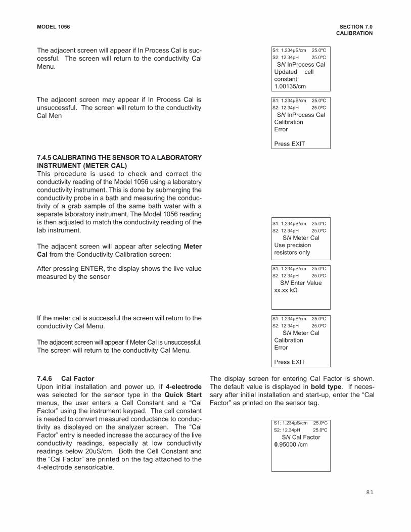
MODEL 1056 SECTION 7.0
CALIBRATION
7.4.5 CALIBRATING THE SENSOR TO A LABORATORY
INSTRUMENT (METER CAL)
This procedure is used to check and correct the
conductivity reading of the Model 1056 using a laboratory
conductivity instrument. This is done by submerging the
conductivity probe in a bath and measuring the conduc
tivity of a grab sample of the same bath water with a
separate laboratory instrument. The Model 1056 reading
is then adjusted to match the conductivity reading of the
lab instrument.
The adjacent screen will appear after selecting Meter
Cal from the Conductivity Calibration screen:
S1: 1.234µS/cm 25.0ºC
S2: 12.34pH 25.0ºC
SN Meter Cal
Use precision
resistors only
The adjacent screen will appear if In Process Cal is suc
cessful. The screen will return to the conductivity Cal
Menu.
The adjacent screen may appear if In Process Cal is
unsuccessful. The screen will return to the conductivity
Cal Men
S1: 1.234µS/cm 25.0ºC
S2: 12.34pH 25.0ºC
SN InProcess Cal
Calibration
Error
Press EXIT
S1: 1.234µS/cm 25.0ºC
S2: 12.34pH 25.0ºC
SN InProcess Cal
Updated cell
constant:
1.00135/cm
After pressing ENTER, the display shows the live value
measured by the sensor
If the meter cal is successful the screen will return to the
conductivity Cal Menu.
The adjacent screen will appear if Meter Cal is unsuccessful.
The screen will return to the conductivity Cal Menu.
S1: 1.234µS/cm 25.0ºC
S2: 12.34pH 25.0ºC
SN Meter Cal
Calibration
Error
Press EXIT
S1: 1.234µS/cm 25.0ºC
S2: 12.34pH 25.0ºC
SN Enter Value
xx.xx kΩ
7.4.6 Cal Factor
Upon initial installation and power up, if 4electrode
was selected for the sensor type in the Quick Start
menus, the user enters a Cell Constant and a “Cal
Factor” using the instrument keypad. The cell constant
is needed to convert measured conductance to conduc
tivity as displayed on the analyzer screen. The “Cal
Factor” entry is needed increase the accuracy of the live
conductivity readings, especially at low conductivity
readings below 20uS/cm. Both the Cell Constant and
the “Cal Factor” are printed on the tag attached to the
4electrode sensor/cable.
The display screen for entering Cal Factor is shown.
The default value is displayed in bold type. If neces
sary after initial installation and startup, enter the “Cal
Factor” as printed on the sensor tag.
S1: 1.234µS/cm 25.0ºC
S2: 12.34pH 25.0ºC
SN Cal Factor
0.95000 /cm
81
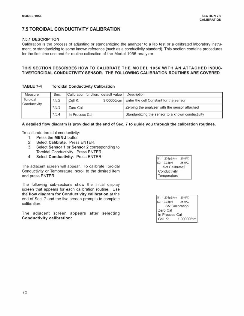
The following subsections show the initial display
screen that appears for each calibration routine. Use
the flow diagram for Conductivity calibration at the
end of Sec. 7 and the live screen prompts to complete
calibration.
The adjacent screen appears after selecting
Conductivity calibration:
S1: 1.234µS/cm 25.0ºC
S2: 12.34pH 25.0ºC
SN Calibration
Zero Cal
In Process Cal
Cell K: 1.00000/cm
MODEL 1056 SECTION 7.0
CALIBRATION
To calibrate toroidal conductivity:
1. Press the MENU button
2. Select Calibrate. Press ENTER.
3. Select Sensor 1 or Sensor 2 corresponding to
Toroidal Conductivity. Press ENTER.
4. Select Conductivity. Press ENTER.
The adjacent screen will appear. To calibrate Toroidal
Conductivity or Temperature, scroll to the desired item
and press ENTER
S1: 1.234µS/cm 25.0ºC
S2: 12.34pH 25.0ºC
SN Calibrate?
Conductivity
Temperature
Measure Sec. Calibration function: default value Description
Toroidal
Conductivity7.5.2 Cell K: 3.00000/cm Enter the cell Constant for the sensor
7.5.3 Zero Cal Zeroing the analyzer with the sensor attached
7.5.4 In Process Cal Standardizing the sensor to a known conductivity
A detailed flow diagram is provided at the end of Sec. 7 to guide you through the calibration routines.
TABLE 74 Toroidal Conductivity Calibration
7.5 TOROIDAL CONDUCTIVITY CALIBRATION
7.5.1 DESCRIPTION
Calibration is the process of adjusting or standardizing the analyzer to a lab test or a calibrated laboratory instru
ment, or standardizing to some known reference (such as a conductivity standard). This section contains procedures
for the first time use and for routine calibration of the Model 1056 analyzer.
THIS SECTION DESCRIBES HOW TO CALIBRATE THE MODEL 1056 WITH AN ATTACHED INDUC
TIVE/TOROIDAL CONDUCTIVITY SENSOR. THE FOLLOWING CALIBRATION ROUTINES ARE COVERED
82
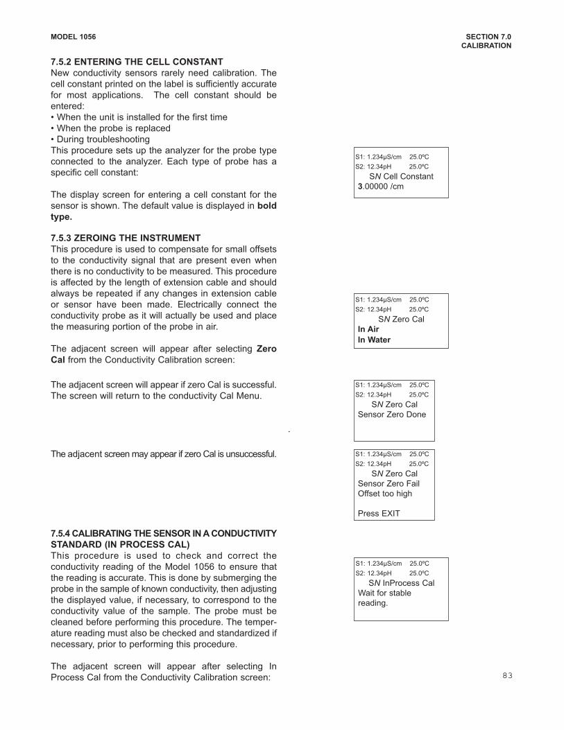
7.5.4 CALIBRATING THE SENSOR IN A CONDUCTIVITY
STANDARD (IN PROCESS CAL)
This procedure is used to check and correct the
conductivity reading of the Model 1056 to ensure that
the reading is accurate. This is done by submerging the
probe in the sample of known conductivity, then adjusting
the displayed value, if necessary, to correspond to the
conductivity value of the sample. The probe must be
cleaned before performing this procedure. The temper
ature reading must also be checked and standardized if
necessary, prior to performing this procedure.
The adjacent screen will appear after selecting In
Process Cal from the Conductivity Calibration screen:
MODEL 1056 SECTION 7.0
CALIBRATION
7.5.2 ENTERING THE CELL CONSTANT
New conductivity sensors rarely need calibration. The
cell constant printed on the label is sufficiently accurate
for most applications. The cell constant should be
entered:
• When the unit is installed for the first time
• When the probe is replaced
• During troubleshooting
This procedure sets up the analyzer for the probe type
connected to the analyzer. Each type of probe has a
specific cell constant:
The display screen for entering a cell constant for the
sensor is shown. The default value is displayed in bold
type.
S1: 1.234µS/cm 25.0ºC
S2: 12.34pH 25.0ºC
SN Cell Constant
3.00000 /cm
7.5.3 ZEROING THE INSTRUMENT
This procedure is used to compensate for small offsets
to the conductivity signal that are present even when
there is no conductivity to be measured. This procedure
is affected by the length of extension cable and should
always be repeated if any changes in extension cable
or sensor have been made. Electrically connect the
conductivity probe as it will actually be used and place
the measuring portion of the probe in air.
The adjacent screen will appear after selecting Zero
Cal from the Conductivity Calibration screen:
S1: 1.234µS/cm 25.0ºC
S2: 12.34pH 25.0ºC
SN Zero Cal
In Air
In Water
The adjacent screen will appear if zero Cal is successful.
The screen will return to the conductivity Cal Menu.
.
The adjacent screen may appear if zero Cal is unsuccessful. S1: 1.234µS/cm 25.0ºC
S2: 12.34pH 25.0ºC
SN Zero Cal
Sensor Zero Fail
Offset too high
Press EXIT
S1: 1.234µS/cm 25.0ºC
S2: 12.34pH 25.0ºC
SN Zero Cal
Sensor Zero Done
S1: 1.234µS/cm 25.0ºC
S2: 12.34pH 25.0ºC
SN InProcess Cal
Wait for stable
reading.
83
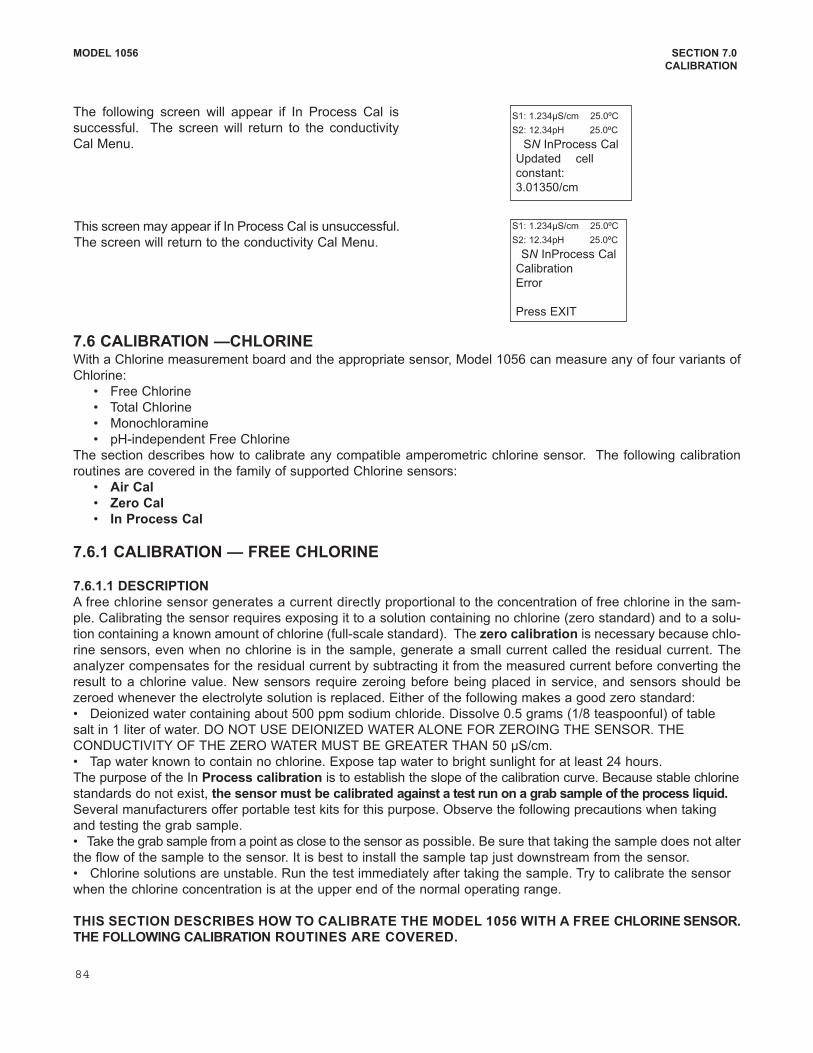
MODEL 1056 SECTION 7.0
CALIBRATION
The following screen will appear if In Process Cal is
successful. The screen will return to the conductivity
Cal Menu.
This screen may appear if In Process Cal is unsuccessful.
The screen will return to the conductivity Cal Menu.
S1: 1.234µS/cm 25.0ºC
S2: 12.34pH 25.0ºC
SN InProcess Cal
Calibration
Error
Press EXIT
S1: 1.234µS/cm 25.0ºC
S2: 12.34pH 25.0ºC
SN InProcess Cal
Updated cell
constant:
3.01350/cm
7.6 CALIBRATION —CHLORINEWith a Chlorine measurement board and the appropriate sensor, Model 1056 can measure any of four variants of
Chlorine:
• Free Chlorine
• Total Chlorine
• Monochloramine
• pHindependent Free Chlorine
The section describes how to calibrate any compatible amperometric chlorine sensor. The following calibration
routines are covered in the family of supported Chlorine sensors:
• Air Cal
• Zero Cal
• In Process Cal
7.6.1 CALIBRATION — FREE CHLORINE
7.6.1.1 DESCRIPTION
A free chlorine sensor generates a current directly proportional to the concentration of free chlorine in the sam
ple. Calibrating the sensor requires exposing it to a solution containing no chlorine (zero standard) and to a solu
tion containing a known amount of chlorine (fullscale standard). The zero calibration is necessary because chlo
rine sensors, even when no chlorine is in the sample, generate a small current called the residual current. The
analyzer compensates for the residual current by subtracting it from the measured current before converting the
result to a chlorine value. New sensors require zeroing before being placed in service, and sensors should be
zeroed whenever the electrolyte solution is replaced. Either of the following makes a good zero standard:
• Deionized water containing about 500 ppm sodium chloride. Dissolve 0.5 grams (1/8 teaspoonful) of table
salt in 1 liter of water. DO NOT USE DEIONIZED WATER ALONE FOR ZEROING THE SENSOR. THE
CONDUCTIVITY OF THE ZERO WATER MUST BE GREATER THAN 50 μS/cm.
• Tap water known to contain no chlorine. Expose tap water to bright sunlight for at least 24 hours.
The purpose of the In Process calibration is to establish the slope of the calibration curve. Because stable chlorine
standards do not exist, the sensor must be calibrated against a test run on a grab sample of the process liquid.
Several manufacturers offer portable test kits for this purpose. Observe the following precautions when taking
and testing the grab sample.
• Take the grab sample from a point as close to the sensor as possible. Be sure that taking the sample does not alter
the flow of the sample to the sensor. It is best to install the sample tap just downstream from the sensor.
• Chlorine solutions are unstable. Run the test immediately after taking the sample. Try to calibrate the sensor
when the chlorine concentration is at the upper end of the normal operating range.
THIS SECTION DESCRIBES HOW TO CALIBRATE THE MODEL 1056 WITH A FREE CHLORINE SENSOR.
THE FOLLOWING CALIBRATION ROUTINES ARE COVERED.
84
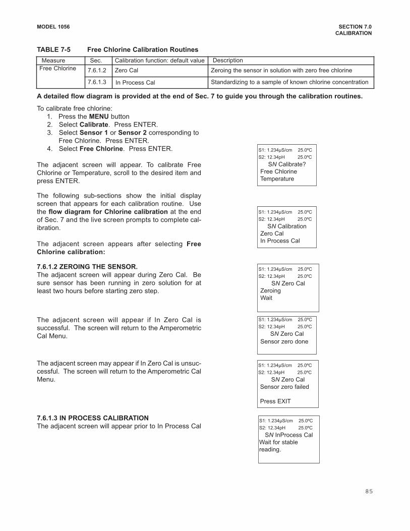
MODEL 1056 SECTION 7.0
CALIBRATION
To calibrate free chlorine:
1. Press the MENU button
2. Select Calibrate. Press ENTER.
3. Select Sensor 1 or Sensor 2 corresponding to
Free Chlorine. Press ENTER.
4. Select Free Chlorine. Press ENTER.
The adjacent screen will appear. To calibrate Free
Chlorine or Temperature, scroll to the desired item and
press ENTER.
S1: 1.234µS/cm 25.0ºC
S2: 12.34pH 25.0ºC
SN Calibrate?
Free Chlorine
Temperature
The following subsections show the initial display
screen that appears for each calibration routine. Use
the flow diagram for Chlorine calibration at the end
of Sec. 7 and the live screen prompts to complete cal
ibration.
The adjacent screen appears after selecting Free
Chlorine calibration:
S1: 1.234µS/cm 25.0ºC
S2: 12.34pH 25.0ºC
SN Calibration
Zero Cal
In Process Cal
7.6.1.2 ZEROING THE SENSOR.
The adjacent screen will appear during Zero Cal. Be
sure sensor has been running in zero solution for at
least two hours before starting zero step.
The adjacent screen will appear if In Zero Cal is
successful. The screen will return to the Amperometric
Cal Menu.
S1: 1.234µS/cm 25.0ºC
S2: 12.34pH 25.0ºC
SN Zero Cal
Sensor zero done
S1: 1.234µS/cm 25.0ºC
S2: 12.34pH 25.0ºC
SN Zero Cal
Zeroing
Wait
Measure Sec. Calibration function: default value Description
Free Chlorine 7.6.1.2 Zero Cal Zeroing the sensor in solution with zero free chlorine
7.6.1.3 In Process Cal Standardizing to a sample of known chlorine concentration
A detailed flow diagram is provided at the end of Sec. 7 to guide you through the calibration routines.
TABLE 75 Free Chlorine Calibration Routines
The adjacent screen may appear if In Zero Cal is unsuc
cessful. The screen will return to the Amperometric Cal
Menu.
S1: 1.234µS/cm 25.0ºC
S2: 12.34pH 25.0ºC
SN Zero Cal
Sensor zero failed
Press EXIT
7.6.1.3 IN PROCESS CALIBRATION
The adjacent screen will appear prior to In Process CalS1: 1.234µS/cm 25.0ºC
S2: 12.34pH 25.0ºC
SN InProcess Cal
Wait for stable
reading.
85
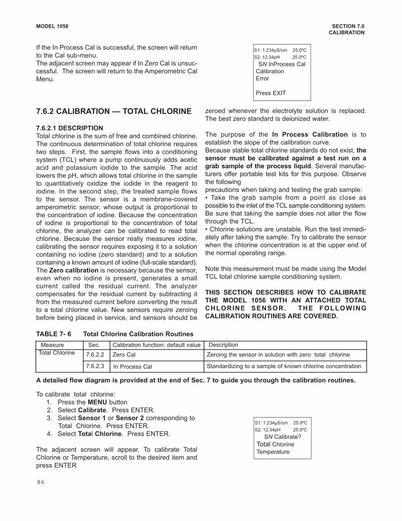
MODEL 1056 SECTION 7.0
CALIBRATION
7.6.2 CALIBRATION — TOTAL CHLORINE
7.6.2.1 DESCRIPTION
Total chlorine is the sum of free and combined chlorine.
The continuous determination of total chlorine requires
two steps. First, the sample flows into a conditioning
system (TCL) where a pump continuously adds acetic
acid and potassium iodide to the sample. The acid
lowers the pH, which allows total chlorine in the sample
to quantitatively oxidize the iodide in the reagent to
iodine. In the second step, the treated sample flows
to the sensor. The sensor is a membranecovered
amperometric sensor, whose output is proportional to
the concentration of iodine. Because the concentration
of iodine is proportional to the concentration of total
chlorine, the analyzer can be calibrated to read total
chlorine. Because the sensor really measures iodine,
calibrating the sensor requires exposing it to a solution
containing no iodine (zero standard) and to a solution
containing a known amount of iodine (fullscale standard).
The Zero calibration is necessary because the sensor,
even when no iodine is present, generates a small
current called the residual current. The analyzer
compensates for the residual current by subtracting it
from the measured current before converting the result
to a total chlorine value. New sensors require zeroing
before being placed in service, and sensors should be
zeroed whenever the electrolyte solution is replaced.
The best zero standard is deionized water.
The purpose of the In Process Calibration is to
establish the slope of the calibration curve.
Because stable total chlorine standards do not exist, the
sensor must be calibrated against a test run on a
grab sample of the process liquid. Several manufac
turers offer portable test kits for this purpose. Observe
the following
precautions when taking and testing the grab sample:
• Take the grab sample from a point as close as
possible to the inlet of the TCL sample conditioning system.
Be sure that taking the sample does not alter the flow
through the TCL.
• Chlorine solutions are unstable. Run the test immedi
ately after taking the sample. Try to calibrate the sensor
when the chlorine concentration is at the upper end of
the normal operating range.
Note this measurement must be made using the Model
TCL total chlorine sample conditioning system.
THIS SECTION DESCRIBES HOW TO CALIBRATE
THE MODEL 1056 WITH AN ATTACHED TOTAL
CHLORINE SENSOR. THE FOLLOWING
CALIBRATION ROUTINES ARE COVERED.
Measure Sec. Calibration function: default value Description
Total Chlorine 7.6.2.2 Zero Cal Zeroing the sensor in solution with zero total chlorine
7.6.2.3 In Process Cal Standardizing to a sample of known chlorine concentration
A detailed flow diagram is provided at the end of Sec. 7 to guide you through the calibration routines.
TABLE 7 6 Total Chlorine Calibration Routines
To calibrate total chlorine:
1. Press the MENU button
2. Select Calibrate. Press ENTER.
3. Select Sensor 1 or Sensor 2 corresponding to
Total Chlorine. Press ENTER.
4. Select Total Chlorine. Press ENTER.
The adjacent screen will appear. To calibrate Total
Chlorine or Temperature, scroll to the desired item and
press ENTER
S1: 1.234µS/cm 25.0ºC
S2: 12.34pH 25.0ºC
SN Calibrate?
Total Chlorine
Temperature
If the In Process Cal is successful, the screen will return
to the Cal submenu.
The adjacent screen may appear if In Zero Cal is unsuc
cessful. The screen will return to the Amperometric Cal
Menu.
S1: 1.234µS/cm 25.0ºC
S2: 12.34pH 25.0ºC
SN InProcess Cal
Calibration
Error
Press EXIT
86
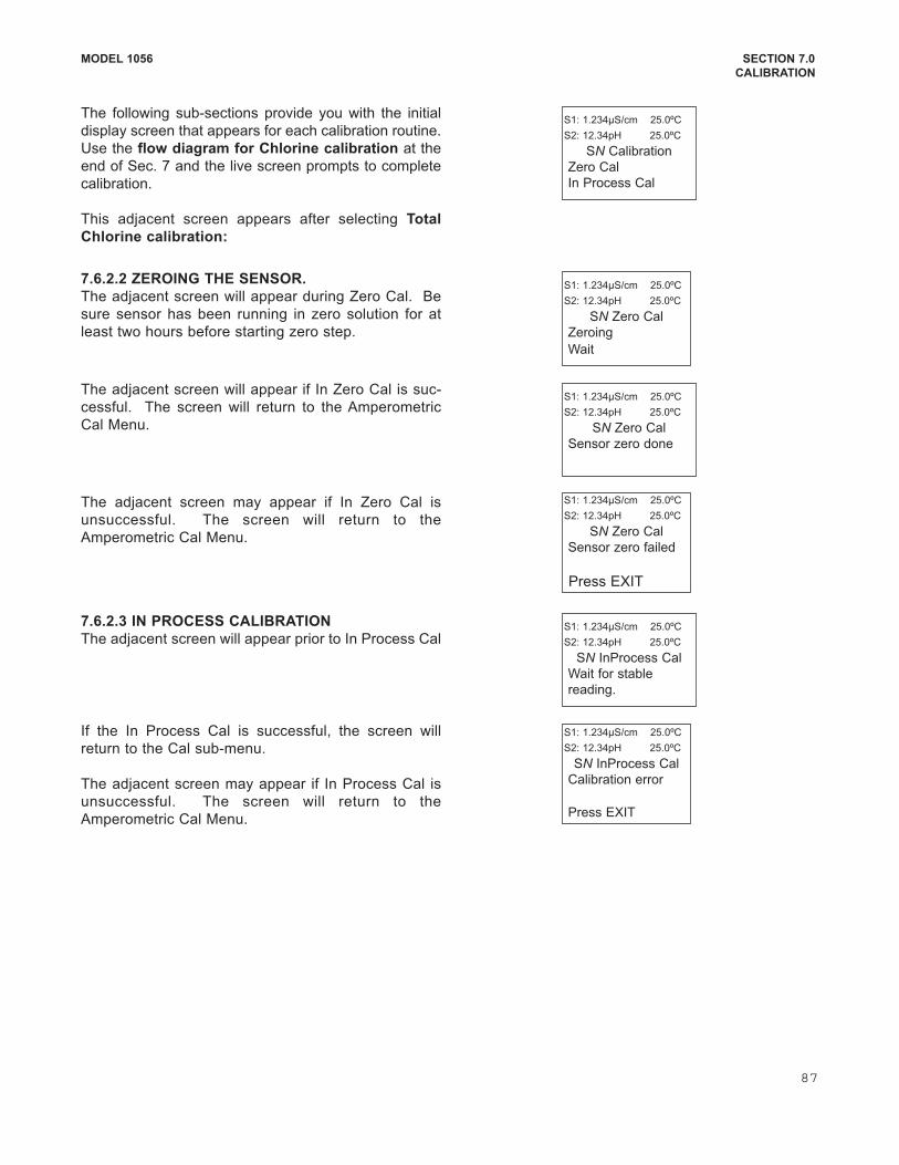
MODEL 1056 SECTION 7.0
CALIBRATION
The following subsections provide you with the initial
display screen that appears for each calibration routine.
Use the flow diagram for Chlorine calibration at the
end of Sec. 7 and the live screen prompts to complete
calibration.
This adjacent screen appears after selecting Total
Chlorine calibration:
7.6.2.2 ZEROING THE SENSOR.
The adjacent screen will appear during Zero Cal. Be
sure sensor has been running in zero solution for at
least two hours before starting zero step.
S1: 1.234µS/cm 25.0ºC
S2: 12.34pH 25.0ºC
SN Zero Cal
Zeroing
Wait
S1: 1.234µS/cm 25.0ºC
S2: 12.34pH 25.0ºC
SN Calibration
Zero Cal
In Process Cal
The adjacent screen may appear if In Zero Cal is
unsuccessful. The screen will return to the
Amperometric Cal Menu.
S1: 1.234µS/cm 25.0ºC
S2: 12.34pH 25.0ºC
SN Zero Cal
Sensor zero failed
Press EXIT
7.6.2.3 IN PROCESS CALIBRATION
The adjacent screen will appear prior to In Process Cal
If the In Process Cal is successful, the screen will
return to the Cal submenu.
The adjacent screen may appear if In Process Cal is
unsuccessful. The screen will return to the
Amperometric Cal Menu.
S1: 1.234µS/cm 25.0ºC
S2: 12.34pH 25.0ºC
SN InProcess Cal
Calibration error
Press EXIT
S1: 1.234µS/cm 25.0ºC
S2: 12.34pH 25.0ºC
SN InProcess Cal
Wait for stable
reading.
The adjacent screen will appear if In Zero Cal is suc
cessful. The screen will return to the Amperometric
Cal Menu.
S1: 1.234µS/cm 25.0ºC
S2: 12.34pH 25.0ºC
SN Zero Cal
Sensor zero done
87
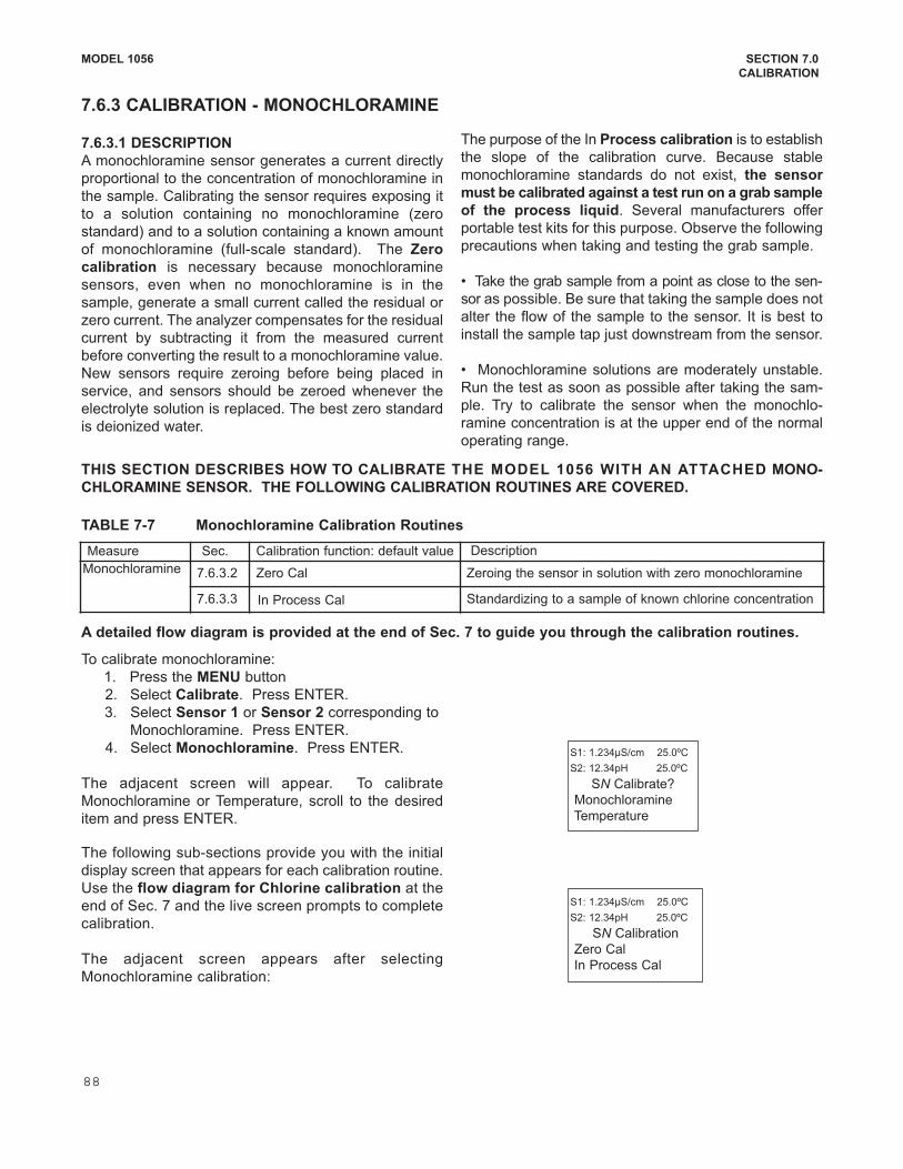
MODEL 1056 SECTION 7.0
CALIBRATION
The following subsections provide you with the initial
display screen that appears for each calibration routine.
Use the flow diagram for Chlorine calibration at the
end of Sec. 7 and the live screen prompts to complete
calibration.
The adjacent screen appears after selecting
Monochloramine calibration:
S1: 1.234µS/cm 25.0ºC
S2: 12.34pH 25.0ºC
SN Calibration
Zero Cal
In Process Cal
7.6.3 CALIBRATION MONOCHLORAMINE
7.6.3.1 DESCRIPTION
A monochloramine sensor generates a current directly
proportional to the concentration of monochloramine in
the sample. Calibrating the sensor requires exposing it
to a solution containing no monochloramine (zero
standard) and to a solution containing a known amount
of monochloramine (fullscale standard). The Zero
calibration is necessary because monochloramine
sensors, even when no monochloramine is in the
sample, generate a small current called the residual or
zero current. The analyzer compensates for the residual
current by subtracting it from the measured current
before converting the result to a monochloramine value.
New sensors require zeroing before being placed in
service, and sensors should be zeroed whenever the
electrolyte solution is replaced. The best zero standard
is deionized water.
The purpose of the In Process calibration is to establish
the slope of the calibration curve. Because stable
monochloramine standards do not exist, the sensor
must be calibrated against a test run on a grab sample
of the process liquid. Several manufacturers offer
portable test kits for this purpose. Observe the following
precautions when taking and testing the grab sample.
• Take the grab sample from a point as close to the sen
sor as possible. Be sure that taking the sample does not
alter the flow of the sample to the sensor. It is best to
install the sample tap just downstream from the sensor.
• Monochloramine solutions are moderately unstable.
Run the test as soon as possible after taking the sam
ple. Try to calibrate the sensor when the monochlo
ramine concentration is at the upper end of the normal
operating range.
Measure Sec. Calibration function: default value Description
Monochloramine 7.6.3.2 Zero Cal Zeroing the sensor in solution with zero monochloramine
7.6.3.3 In Process Cal Standardizing to a sample of known chlorine concentration
A detailed flow diagram is provided at the end of Sec. 7 to guide you through the calibration routines.
To calibrate monochloramine:
1. Press the MENU button
2. Select Calibrate. Press ENTER.
3. Select Sensor 1 or Sensor 2 corresponding to
Monochloramine. Press ENTER.
4. Select Monochloramine. Press ENTER.
The adjacent screen will appear. To calibrate
Monochloramine or Temperature, scroll to the desired
item and press ENTER.
S1: 1.234µS/cm 25.0ºC
S2: 12.34pH 25.0ºC
SN Calibrate?
Monochloramine
Temperature
TABLE 77 Monochloramine Calibration Routines
THIS SECTION DESCRIBES HOW TO CALIBRATE THE MODEL 1056 WITH AN ATTACHED MONO
CHLORAMINE SENSOR. THE FOLLOWING CALIBRATION ROUTINES ARE COVERED.
88
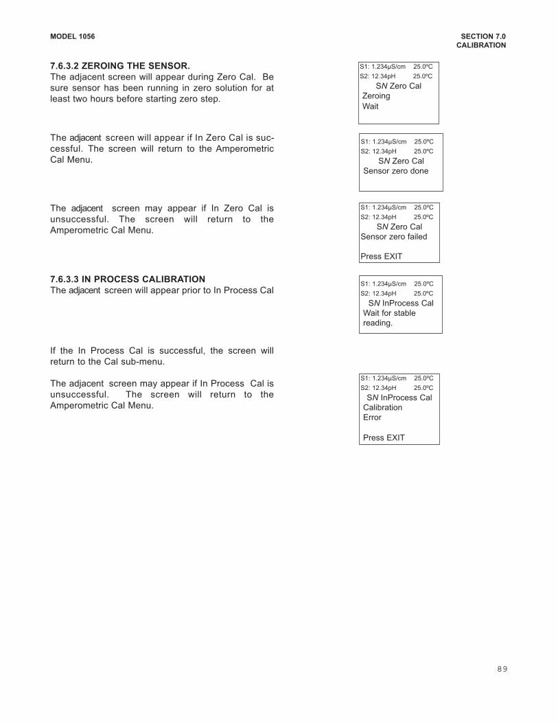
MODEL 1056 SECTION 7.0
CALIBRATION
7.6.3.2 ZEROING THE SENSOR.
The adjacent screen will appear during Zero Cal. Be
sure sensor has been running in zero solution for at
least two hours before starting zero step.
S1: 1.234µS/cm 25.0ºC
S2: 12.34pH 25.0ºC
SN Zero Cal
Zeroing
Wait
The adjacent screen may appear if In Zero Cal is
unsuccessful. The screen will return to the
Amperometric Cal Menu.
The adjacent screen will appear if In Zero Cal is suc
cessful. The screen will return to the Amperometric
Cal Menu.
S1: 1.234µS/cm 25.0ºC
S2: 12.34pH 25.0ºC
SN Zero Cal
Sensor zero failed
Press EXIT
S1: 1.234µS/cm 25.0ºC
S2: 12.34pH 25.0ºC
SN Zero Cal
Sensor zero done
If the In Process Cal is successful, the screen will
return to the Cal submenu.
The adjacent screen may appear if In Process Cal is
unsuccessful. The screen will return to the
Amperometric Cal Menu.
7.6.3.3 IN PROCESS CALIBRATION
The adjacent screen will appear prior to In Process Cal
S1: 1.234µS/cm 25.0ºC
S2: 12.34pH 25.0ºC
SN InProcess Cal
Calibration
Error
Press EXIT
S1: 1.234µS/cm 25.0ºC
S2: 12.34pH 25.0ºC
SN InProcess Cal
Wait for stable
reading.
89
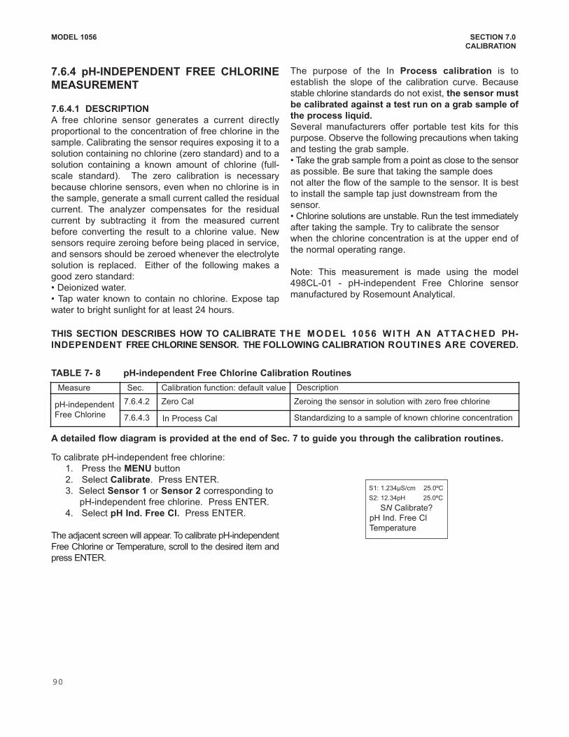
MODEL 1056 SECTION 7.0
CALIBRATION
7.6.4 pHINDEPENDENT FREE CHLORINE
MEASUREMENT
7.6.4.1 DESCRIPTION
A free chlorine sensor generates a current directly
proportional to the concentration of free chlorine in the
sample. Calibrating the sensor requires exposing it to a
solution containing no chlorine (zero standard) and to a
solution containing a known amount of chlorine (full
scale standard). The zero calibration is necessary
because chlorine sensors, even when no chlorine is in
the sample, generate a small current called the residual
current. The analyzer compensates for the residual
current by subtracting it from the measured current
before converting the result to a chlorine value. New
sensors require zeroing before being placed in service,
and sensors should be zeroed whenever the electrolyte
solution is replaced. Either of the following makes a
good zero standard:
• Deionized water.
• Tap water known to contain no chlorine. Expose tap
water to bright sunlight for at least 24 hours.
The purpose of the In Process calibration is to
establish the slope of the calibration curve. Because
stable chlorine standards do not exist, the sensor must
be calibrated against a test run on a grab sample of
the process liquid.
Several manufacturers offer portable test kits for this
purpose. Observe the following precautions when taking
and testing the grab sample.
• Take the grab sample from a point as close to the sensor
as possible. Be sure that taking the sample does
not alter the flow of the sample to the sensor. It is best
to install the sample tap just downstream from the
sensor.
• Chlorine solutions are unstable. Run the test immediately
after taking the sample. Try to calibrate the sensor
when the chlorine concentration is at the upper end of
the normal operating range.
Note: This measurement is made using the model
498CL01 pHindependent Free Chlorine sensor
manufactured by Rosemount Analytical.
Measure Sec. Calibration function: default value Description
pHindependent
Free Chlorine
7.6.4.2 Zero Cal Zeroing the sensor in solution with zero free chlorine
7.6.4.3 In Process Cal Standardizing to a sample of known chlorine concentration
A detailed flow diagram is provided at the end of Sec. 7 to guide you through the calibration routines.
TABLE 7 8 pHindependent Free Chlorine Calibration Routines
To calibrate pHindependent free chlorine:
1. Press the MENU button
2. Select Calibrate. Press ENTER.
3. Select Sensor 1 or Sensor 2 corresponding to
pHindependent free chlorine. Press ENTER.
4. Select pH Ind. Free Cl. Press ENTER.
The adjacent screen will appear. To calibrate pHindependent
Free Chlorine or Temperature, scroll to the desired item and
press ENTER.
S1: 1.234µS/cm 25.0ºC
S2: 12.34pH 25.0ºC
SN Calibrate?
pH Ind. Free Cl
Temperature
THIS SECTION DESCRIBES HOW TO CALIBRATE THE MODEL 1056 WITH AN ATTACHED PH
INDEPENDENT FREE CHLORINE SENSOR. THE FOLLOWING CALIBRATION ROUTINES ARE COVERED.
90

MODEL 1056 SECTION 7.0
CALIBRATION
The following subsections provide you with the initial
display screen that appears for each calibration
routine. Use the flow diagram for Chlorine
calibration at the end of Sec. 7 and the live screen
prompts to complete calibration.
The adjacent screen appears after selecting pHinde
pendent free chlorine calibration:
7.6.4.2 ZEROING THE SENSOR.
The adjacent screen will appear during Zero Cal S1: 1.234µS/cm 25.0ºC
S2: 12.34pH 25.0ºC
SN Zero Cal
Zeroing
Wait
S1: 1.234µS/cm 25.0ºC
S2: 12.34pH 25.0ºC
SN Calibration
Zero Cal
In Process Cal
The adjacent screen may appear if In Zero Cal is
unsuccessful. The screen will return to the
Amperometric Cal Menu.
The adjacent screen will appear if In Zero Cal is suc
cessful. The screen will return to the Amperometric
Cal Menu.
S1: 1.234µS/cm 25.0ºC
S2: 12.34pH 25.0ºC
SN Zero Cal
Sensor zero failed
Press EXIT
S1: 1.234µS/cm 25.0ºC
S2: 12.34pH 25.0ºC
SN Zero Cal
Sensor zero done
If the In Process Cal is successful, the screen will
return to the Cal submenu.
The adjacent screen may appear if In Process Cal is
unsuccessful. The screen will return to the
Amperometric Cal Menu.
7.6.4.3 IN PROCESS CALIBRATION
The following screen will appear prior to In Process Cal
S1: 1.234µS/cm 25.0ºC
S2: 12.34pH 25.0ºC
SN InProcess Cal
Calibration
Error
Press EXIT
S1: 1.234µS/cm 25.0ºC
S2: 12.34pH 25.0ºC
SN InProcess Cal
Wait for stable
reading.
91
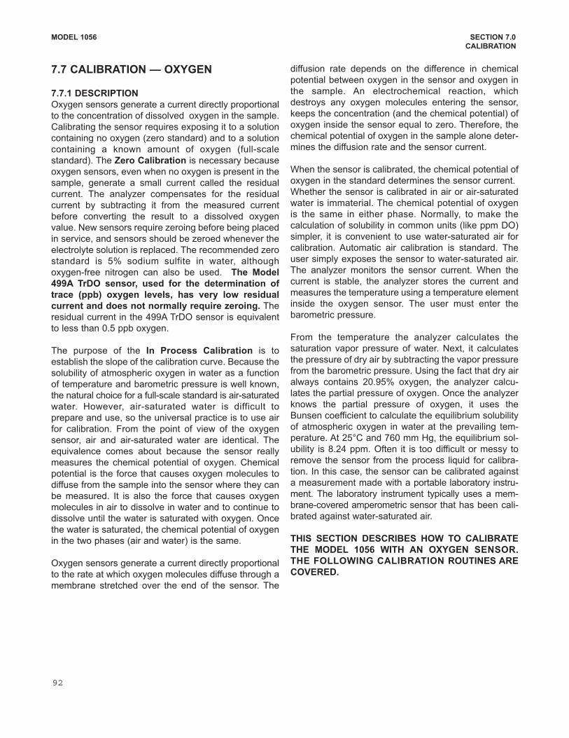
MODEL 1056 SECTION 7.0
CALIBRATION
7.7 CALIBRATION — OXYGEN
7.7.1 DESCRIPTION
Oxygen sensors generate a current directly proportional
to the concentration of dissolved oxygen in the sample.
Calibrating the sensor requires exposing it to a solution
containing no oxygen (zero standard) and to a solution
containing a known amount of oxygen (fullscale
standard). The Zero Calibration is necessary because
oxygen sensors, even when no oxygen is present in the
sample, generate a small current called the residual
current. The analyzer compensates for the residual
current by subtracting it from the measured current
before converting the result to a dissolved oxygen
value. New sensors require zeroing before being placed
in service, and sensors should be zeroed whenever the
electrolyte solution is replaced. The recommended zero
standard is 5% sodium sulfite in water, although
oxygenfree nitrogen can also be used. The Model
499A TrDO sensor, used for the determination of
trace (ppb) oxygen levels, has very low residual
current and does not normally require zeroing. The
residual current in the 499A TrDO sensor is equivalent
to less than 0.5 ppb oxygen.
The purpose of the In Process Calibration is to
establish the slope of the calibration curve. Because the
solubility of atmospheric oxygen in water as a function
of temperature and barometric pressure is well known,
the natural choice for a fullscale standard is airsaturated
water. However, airsaturated water is difficult to
prepare and use, so the universal practice is to use air
for calibration. From the point of view of the oxygen
sensor, air and airsaturated water are identical. The
equivalence comes about because the sensor really
measures the chemical potential of oxygen. Chemical
potential is the force that causes oxygen molecules to
diffuse from the sample into the sensor where they can
be measured. It is also the force that causes oxygen
molecules in air to dissolve in water and to continue to
dissolve until the water is saturated with oxygen. Once
the water is saturated, the chemical potential of oxygen
in the two phases (air and water) is the same.
Oxygen sensors generate a current directly proportional
to the rate at which oxygen molecules diffuse through a
membrane stretched over the end of the sensor. The
diffusion rate depends on the difference in chemical
potential between oxygen in the sensor and oxygen in
the sample. An electrochemical reaction, which
destroys any oxygen molecules entering the sensor,
keeps the concentration (and the chemical potential) of
oxygen inside the sensor equal to zero. Therefore, the
chemical potential of oxygen in the sample alone deter
mines the diffusion rate and the sensor current.
When the sensor is calibrated, the chemical potential of
oxygen in the standard determines the sensor current.
Whether the sensor is calibrated in air or airsaturated
water is immaterial. The chemical potential of oxygen
is the same in either phase. Normally, to make the
calculation of solubility in common units (like ppm DO)
simpler, it is convenient to use watersaturated air for
calibration. Automatic air calibration is standard. The
user simply exposes the sensor to watersaturated air.
The analyzer monitors the sensor current. When the
current is stable, the analyzer stores the current and
measures the temperature using a temperature element
inside the oxygen sensor. The user must enter the
barometric pressure.
From the temperature the analyzer calculates the
saturation vapor pressure of water. Next, it calculates
the pressure of dry air by subtracting the vapor pressure
from the barometric pressure. Using the fact that dry air
always contains 20.95% oxygen, the analyzer calcu
lates the partial pressure of oxygen. Once the analyzer
knows the partial pressure of oxygen, it uses the
Bunsen coefficient to calculate the equilibrium solubility
of atmospheric oxygen in water at the prevailing tem
perature. At 25°C and 760 mm Hg, the equilibrium sol
ubility is 8.24 ppm. Often it is too difficult or messy to
remove the sensor from the process liquid for calibra
tion. In this case, the sensor can be calibrated against
a measurement made with a portable laboratory instru
ment. The laboratory instrument typically uses a mem
branecovered amperometric sensor that has been cali
brated against watersaturated air.
THIS SECTION DESCRIBES HOW TO CALIBRATE
THE MODEL 1056 WITH AN OXYGEN SENSOR.
THE FOLLOWING CALIBRATION ROUTINES ARE
COVERED.
92
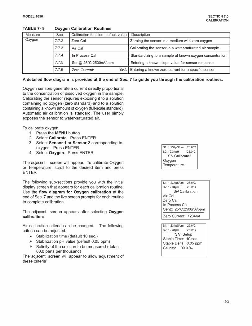
MODEL 1056 SECTION 7.0
CALIBRATION
A detailed flow diagram is provided at the end of Sec. 7 to guide you through the calibration routines.
Oxygen sensors generate a current directly proportional
to the concentration of dissolved oxygen in the sample.
Calibrating the sensor requires exposing it to a solution
containing no oxygen (zero standard) and to a solution
containing a known amount of oxygen (fullscale standard).
Automatic air calibration is standard. The user simply
exposes the sensor to watersaturated air.
To calibrate oxygen:
1. Press the MENU button
2. Select Calibrate. Press ENTER.
3. Select Sensor 1 or Sensor 2 corresponding to
oxygen. Press ENTER.
4. Select Oxygen. Press ENTER.
The adjacent screen will appear. To calibrate Oxygen
or Temperature, scroll to the desired item and press
ENTER
S1: 1.234µS/cm 25.0ºC
S2: 12.34pH 25.0ºC
SN Calibrate?
Oxygen
Temperature
The following subsections provide you with the initial
display screen that appears for each calibration routine.
Use the flow diagram for Oxygen calibration at the
end of Sec. 7 and the live screen prompts for each routine
to complete calibration.
The adjacent screen appears after selecting Oxygen
calibration:
S1: 1.234µS/cm 25.0ºC
S2: 12.34pH 25.0ºC
SN Calibration
Air Cal
Zero Cal
In Process Cal
Sen@ 25°C:2500nA/ppm
Zero Current: 1234nA
Air calibration criteria can be changed. The following
criteria can be adjusted:
Stabilization time (default 10 sec.)
Stabilization pH value (default 0.05 ppm)
Salinity of the solution to be measured (default 00.0 parts per thousand)
The adjacent screen will appear to allow adjustment of
these criteria”
S1: 1.234µS/cm 25.0ºC
S2: 12.34pH 25.0ºC
SN Setup
Stable Time: 10 sec
Stable Delta: 0.05 ppm
Salinity: 00.0 ‰
Measure Sec. Calibration function: default value Description
Oxygen 7.7.2 Zero Cal Zeroing the sensor in a medium with zero oxygen
7.7.3 Air Cal Calibrating the sensor in a watersaturated air sample
7.7.4 In Process Cal Standardizing to a sample of known oxygen concentration
7.7.5 Sen@ 25°C:2500nA/ppm Entering a known slope value for sensor response
7.7.6 Zero Current: 0nA Entering a known zero current for a specific sensor
TABLE 7 9 Oxygen Calibration Routines
93
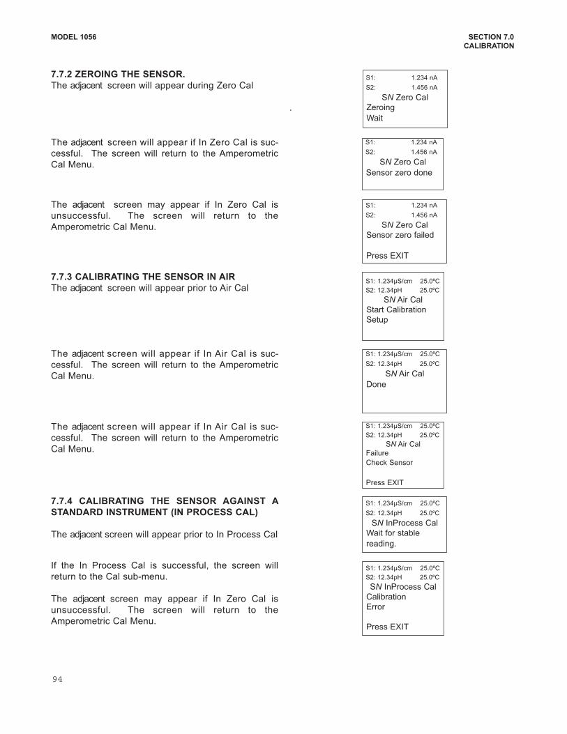
The adjacent screen will appear if In Air Cal is suc
cessful. The screen will return to the Amperometric
Cal Menu.
The adjacent screen will appear if In Air Cal is suc
cessful. The screen will return to the Amperometric
Cal Menu.
S1: 1.234µS/cm 25.0ºC
S2: 12.34pH 25.0ºC
SN Air Cal
Failure
Check Sensor
Press EXIT
S1: 1.234µS/cm 25.0ºC
S2: 12.34pH 25.0ºC
SN Air Cal
Done
If the In Process Cal is successful, the screen will
return to the Cal submenu.
The adjacent screen may appear if In Zero Cal is
unsuccessful. The screen will return to the
Amperometric Cal Menu.
7.7.4 CALIBRATING THE SENSOR AGAINST A
STANDARD INSTRUMENT (IN PROCESS CAL)
The adjacent screen will appear prior to In Process Cal
S1: 1.234µS/cm 25.0ºC
S2: 12.34pH 25.0ºC
SN InProcess Cal
Calibration
Error
Press EXIT
S1: 1.234µS/cm 25.0ºC
S2: 12.34pH 25.0ºC
SN InProcess Cal
Wait for stable
reading.
MODEL 1056 SECTION 7.0
CALIBRATION
The adjacent screen will appear if In Zero Cal is suc
cessful. The screen will return to the Amperometric
Cal Menu.
S1: 1.234 nA
S2: 1.456 nA
SN Zero Cal
Sensor zero done
7.7.3 CALIBRATING THE SENSOR IN AIR
The adjacent screen will appear prior to Air Cal
The adjacent screen may appear if In Zero Cal is
unsuccessful. The screen will return to the
Amperometric Cal Menu.
S1: 1.234µS/cm 25.0ºC
S2: 12.34pH 25.0ºC
SN Air Cal
Start Calibration
Setup
S1: 1.234 nA
S2: 1.456 nA
SN Zero Cal
Sensor zero failed
Press EXIT
7.7.2 ZEROING THE SENSOR.
The adjacent screen will appear during Zero Cal
.
S1: 1.234 nA
S2: 1.456 nA
SN Zero Cal
Zeroing
Wait
94
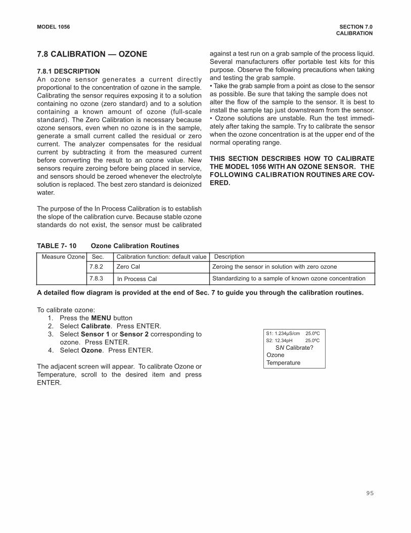
MODEL 1056 SECTION 7.0
CALIBRATION
7.8 CALIBRATION — OZONE
7.8.1 DESCRIPTION
An ozone sensor generates a current directly
proportional to the concentration of ozone in the sample.
Calibrating the sensor requires exposing it to a solution
containing no ozone (zero standard) and to a solution
containing a known amount of ozone (fullscale
standard). The Zero Calibration is necessary because
ozone sensors, even when no ozone is in the sample,
generate a small current called the residual or zero
current. The analyzer compensates for the residual
current by subtracting it from the measured current
before converting the result to an ozone value. New
sensors require zeroing before being placed in service,
and sensors should be zeroed whenever the electrolyte
solution is replaced. The best zero standard is deionized
water.
The purpose of the In Process Calibration is to establish
the slope of the calibration curve. Because stable ozone
standards do not exist, the sensor must be calibrated
against a test run on a grab sample of the process liquid.
Several manufacturers offer portable test kits for this
purpose. Observe the following precautions when taking
and testing the grab sample.
• Take the grab sample from a point as close to the sensor
as possible. Be sure that taking the sample does not
alter the flow of the sample to the sensor. It is best to
install the sample tap just downstream from the sensor.
• Ozone solutions are unstable. Run the test immedi
ately after taking the sample. Try to calibrate the sensor
when the ozone concentration is at the upper end of the
normal operating range.
THIS SECTION DESCRIBES HOW TO CALIBRATE
THE MODEL 1056 WITH AN OZONE SENSOR. THE
FOLLOWING CALIBRATION ROUTINES ARE COV
ERED.
Measure Ozone Sec. Calibration function: default value Description
7.8.2 Zero Cal Zeroing the sensor in solution with zero ozone
7.8.3 In Process Cal Standardizing to a sample of known ozone concentration
A detailed flow diagram is provided at the end of Sec. 7 to guide you through the calibration routines.
TABLE 7 10 Ozone Calibration Routines
To calibrate ozone:
1. Press the MENU button
2. Select Calibrate. Press ENTER.
3. Select Sensor 1 or Sensor 2 corresponding to
ozone. Press ENTER.
4. Select Ozone. Press ENTER.
The adjacent screen will appear. To calibrate Ozone or
Temperature, scroll to the desired item and press
ENTER.
S1: 1.234µS/cm 25.0ºC
S2: 12.34pH 25.0ºC
SN Calibrate?
Ozone
Temperature
95
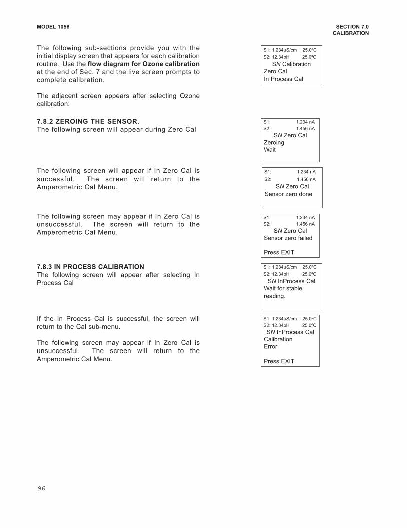
MODEL 1056 SECTION 7.0
CALIBRATION
7.8.2 ZEROING THE SENSOR.
The following screen will appear during Zero Cal
The following subsections provide you with the
initial display screen that appears for each calibration
routine. Use the flow diagram for Ozone calibration
at the end of Sec. 7 and the live screen prompts to
complete calibration.
The adjacent screen appears after selecting Ozone
calibration:
S1: 1.234 nA
S2: 1.456 nA
SN Zero Cal
Zeroing
Wait
S1: 1.234µS/cm 25.0ºC
S2: 12.34pH 25.0ºC
SN Calibration
Zero Cal
In Process Cal
The following screen may appear if In Zero Cal is
unsuccessful. The screen will return to the
Amperometric Cal Menu.
The following screen will appear if In Zero Cal is
successful. The screen will return to the
Amperometric Cal Menu.
S1: 1.234 nA
S2: 1.456 nA
SN Zero Cal
Sensor zero failed
Press EXIT
S1: 1.234 nA
S2: 1.456 nA
SN Zero Cal
Sensor zero done
If the In Process Cal is successful, the screen will
return to the Cal submenu.
The following screen may appear if In Zero Cal is
unsuccessful. The screen will return to the
Amperometric Cal Menu.
7.8.3 IN PROCESS CALIBRATION
The following screen will appear after selecting In
Process Cal
S1: 1.234µS/cm 25.0ºC
S2: 12.34pH 25.0ºC
SN InProcess Cal
Calibration
Error
Press EXIT
S1: 1.234µS/cm 25.0ºC
S2: 12.34pH 25.0ºC
SN InProcess Cal
Wait for stable
reading.
96
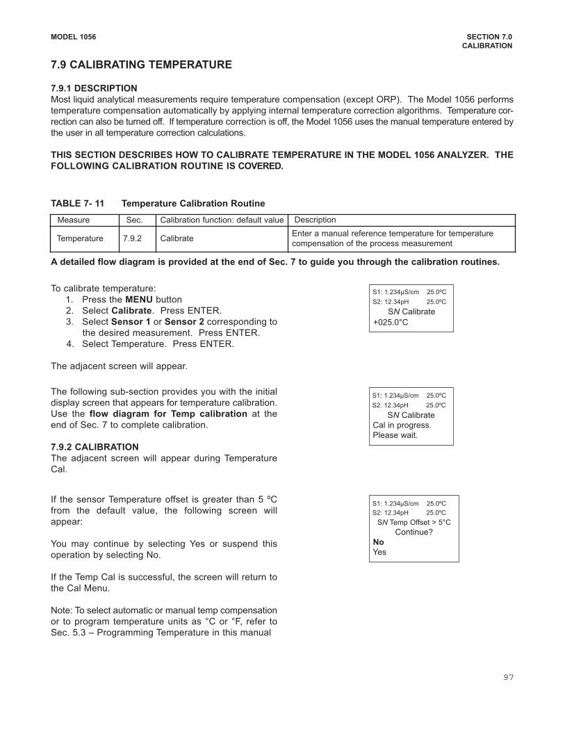
To calibrate temperature:
1. Press the MENU button
2. Select Calibrate. Press ENTER.
3. Select Sensor 1 or Sensor 2 corresponding to
the desired measurement. Press ENTER.
4. Select Temperature. Press ENTER.
The adjacent screen will appear.
Measure Sec. Calibration function: default value Description
Temperature 7.9.2 CalibrateEnter a manual reference temperature for temperature
compensation of the process measurement
A detailed flow diagram is provided at the end of Sec. 7 to guide you through the calibration routines.
S1: 1.234µS/cm 25.0ºC
S2: 12.34pH 25.0ºC
SN Calibrate
+025.0°C
The following subsection provides you with the initial
display screen that appears for temperature calibration.
Use the flow diagram for Temp calibration at the
end of Sec. 7 to complete calibration.
7.9.2 CALIBRATION
The adjacent screen will appear during Temperature
Cal.
If the sensor Temperature offset is greater than 5 ºC
from the default value, the following screen will
appear:
You may continue by selecting Yes or suspend this
operation by selecting No.
If the Temp Cal is successful, the screen will return to
the Cal Menu.
Note: To select automatic or manual temp compensation
or to program temperature units as °C or °F, refer to
Sec. 5.3 – Programming Temperature in this manual
S1: 1.234µS/cm 25.0ºC
S2: 12.34pH 25.0ºC
SN Temp Offset > 5°C
Continue?
No
Yes
S1: 1.234µS/cm 25.0ºC
S2: 12.34pH 25.0ºC
SN Calibrate
Cal in progress.
Please wait.
TABLE 7 11 Temperature Calibration Routine
MODEL 1056 SECTION 7.0
CALIBRATION
7.9 CALIBRATING TEMPERATURE
7.9.1 DESCRIPTION
Most liquid analytical measurements require temperature compensation (except ORP). The Model 1056 performs
temperature compensation automatically by applying internal temperature correction algorithms. Temperature cor
rection can also be turned off. If temperature correction is off, the Model 1056 uses the manual temperature entered by
the user in all temperature correction calculations.
THIS SECTION DESCRIBES HOW TO CALIBRATE TEMPERATURE IN THE MODEL 1056 ANALYZER. THE
FOLLOWING CALIBRATION ROUTINE IS COVERED.
97
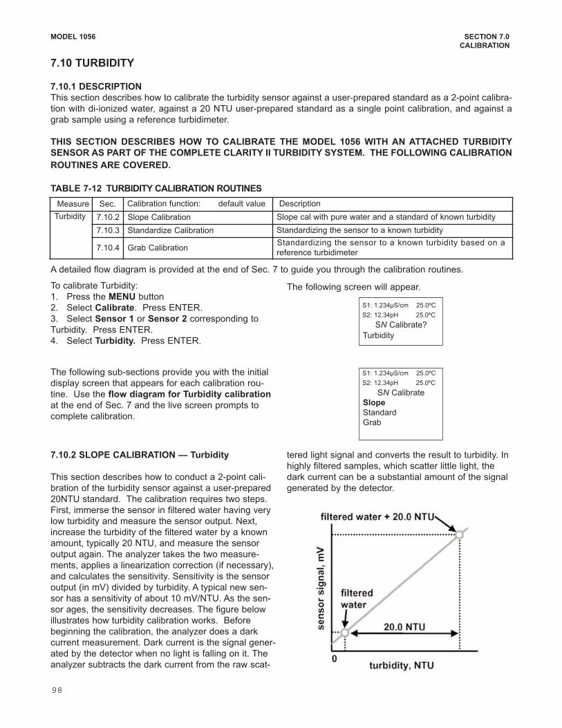
The following subsections provide you with the initial
display screen that appears for each calibration rou
tine. Use the flow diagram for Turbidity calibration
at the end of Sec. 7 and the live screen prompts to
complete calibration.
MODEL 1056 SECTION 7.0
CALIBRATION
7.10 TURBIDITY
7.10.1 DESCRIPTION
This section describes how to calibrate the turbidity sensor against a userprepared standard as a 2point calibra
tion with diionized water, against a 20 NTU userprepared standard as a single point calibration, and against a
grab sample using a reference turbidimeter.
THIS SECTION DESCRIBES HOW TO CALIBRATE THE MODEL 1056 WITH AN ATTACHED TURBIDITY
SENSOR AS PART OF THE COMPLETE CLARITY II TURBIDITY SYSTEM. THE FOLLOWING CALIBRATION
ROUTINES ARE COVERED.
To calibrate Turbidity:
1. Press the MENU button
2. Select Calibrate. Press ENTER.
3. Select Sensor 1 or Sensor 2 corresponding to
Turbidity. Press ENTER.
4. Select Turbidity. Press ENTER.
The following screen will appear.
7.10.2 SLOPE CALIBRATION — Turbidity
This section describes how to conduct a 2point cali
bration of the turbidity sensor against a userprepared
20NTU standard. The calibration requires two steps.
First, immerse the sensor in filtered water having very
low turbidity and measure the sensor output. Next,
increase the turbidity of the filtered water by a known
amount, typically 20 NTU, and measure the sensor
output again. The analyzer takes the two measure
ments, applies a linearization correction (if necessary),
and calculates the sensitivity. Sensitivity is the sensor
output (in mV) divided by turbidity. A typical new sen
sor has a sensitivity of about 10 mV/NTU. As the sen
sor ages, the sensitivity decreases. The figure below
illustrates how turbidity calibration works. Before
beginning the calibration, the analyzer does a dark
current measurement. Dark current is the signal gener
ated by the detector when no light is falling on it. The
analyzer subtracts the dark current from the raw scat
tered light signal and converts the result to turbidity. In
highly filtered samples, which scatter little light, the
dark current can be a substantial amount of the signal
generated by the detector.
A detailed flow diagram is provided at the end of Sec. 7 to guide you through the calibration routines.
Measure Sec. Calibration function: default value Description
Turbidity 7.10.2 Slope Calibration Slope cal with pure water and a standard of known turbidity
7.10.3 Standardize Calibration Standardizing the sensor to a known turbidity
7.10.4 Grab CalibrationStandardizing the sensor to a known turbidity based on a
reference turbidimeter
S1: 1.234µS/cm 25.0ºC
S2: 12.34pH 25.0ºC
SN Calibrate?
Turbidity
S1: 1.234µS/cm 25.0ºC
S2: 12.34pH 25.0ºC
SN Calibrate
Slope
Standard
Grab
98
TABLE 712 TURBIDITY CALIBRATION ROUTINES
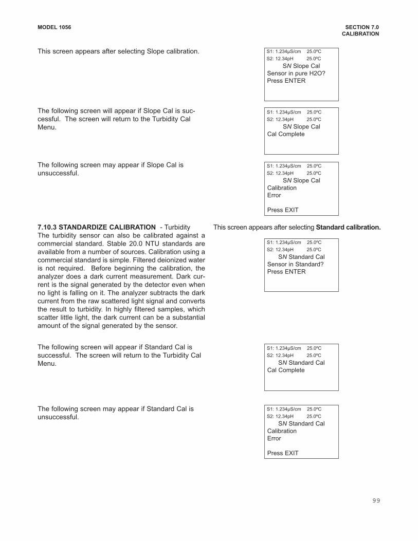
The following screen will appear if Standard Cal is
successful. The screen will return to the Turbidity Cal
Menu.
7.10.3 STANDARDIZE CALIBRATION Turbidity
The turbidity sensor can also be calibrated against a
commercial standard. Stable 20.0 NTU standards are
available from a number of sources. Calibration using a
commercial standard is simple. Filtered deionized water
is not required. Before beginning the calibration, the
analyzer does a dark current measurement. Dark cur
rent is the signal generated by the detector even when
no light is falling on it. The analyzer subtracts the dark
current from the raw scattered light signal and converts
the result to turbidity. In highly filtered samples, which
scatter little light, the dark current can be a substantial
amount of the signal generated by the sensor.
This screen appears after selecting Standard calibration.
The following screen may appear if Slope Cal is
unsuccessful.
This screen appears after selecting Slope calibration.
MODEL 1056 SECTION 7.0
CALIBRATION
The following screen will appear if Slope Cal is suc
cessful. The screen will return to the Turbidity Cal
Menu.
S1: 1.234µS/cm 25.0ºC
S2: 12.34pH 25.0ºC
SN Slope Cal
Sensor in pure H2O?
Press ENTER
S1: 1.234µS/cm 25.0ºC
S2: 12.34pH 25.0ºC
SN Slope Cal
Cal Complete
S1: 1.234µS/cm 25.0ºC
S2: 12.34pH 25.0ºC
SN Standard Cal
Cal Complete
S1: 1.234µS/cm 25.0ºC
S2: 12.34pH 25.0ºC
SN Slope Cal
Calibration
Error
Press EXIT
S1: 1.234µS/cm 25.0ºC
S2: 12.34pH 25.0ºC
SN Standard Cal
Sensor in Standard?
Press ENTER
The following screen may appear if Standard Cal is
unsuccessful.
S1: 1.234µS/cm 25.0ºC
S2: 12.34pH 25.0ºC
SN Standard Cal
Calibration
Error
Press EXIT
99
The following screen may appear if Grab Cal is
unsuccessful.
The following screen will appear if Grab Cal is successful.
The screen will return to the Turbidity Cal Menu.
7.10.4 GRAB CALIBRATION Turbidity
If desired, the turbidity sensor can be calibrated
against the turbidity reading from another instrument.
The analyzer treats the value entered by the user as
though it were the true turbidity of the sample.
Therefore, grab sample calibration changes the sensi
tivity, it does not apply an offset to the reading.
This screen appears after selecting Grab calibration.
To calibrate Pulse Flow:
1. Press the MENU button
2. Select Calibrate. Press ENTER.
3. Select Sensor 1 or Sensor 2 corresponding to
Flow. Press ENTER.
4. Select Pulse Flow. Press ENTER.
The following screen will appear.
A detailed flow diagram is provided at the end of Sec. 7 to guide you through the calibration routines.
MODEL 1056 SECTION 7.0
CALIBRATION
7.11 PULSE FLOW
7.11.1 DESCRIPTION
A variety of pulse flow sensors can be wired to the Flow signal input board to measure flow volume, total volume
and flow difference (if 2 Flow signal boards are installed). The Model 1056 Flow signal board will support flow
sensors that are selfdriven (powered by the rotation of the impeller paddlewheel).
THIS SECTION DESCRIBES HOW TO CALIBRATE THE MODEL 1056 WITH AN ATTACHED FLOW SENSOR.
THE FOLLOWING CALIBRATION ROUTINES ARE COVERED.
S1: 1.234µS/cm 25.0ºC
S2: 12.34pH 25.0ºC
SN Grab Cal
Wait for stable
reading
S1: 1.234µS/cm 25.0ºC
S2: 12.34pH 25.0ºC
SN Grab Cal
Cal Complete
S1: 1.234µS/cm 25.0ºC
S2: 12.34pH 25.0ºC
SN Grab Cal
Calibration
Error
Press EXIT
S1: 1.234µS/cm 25.0ºC
S2: 12.34pH 25.0ºC
SN Calibrate?
Pulse Flow
Measure Sec. Calibration function Description
Pulse
Flow7.11.2 K Factor A constant value representing pulses/Gal of flow
7.11.3 Frequency/Velocity & Pipe Alternate cal method – requires manual entry of frequency (Hz)
per velocity and Pipe diameter used
7.11.4 In process Calibration Calibration based on known volume per unit of time
7.11.5 Totalizer Control User settings to stop, restart and reset total volume meter
TABLE 713 FLOW CALIBRATION ROUTINES
100
MODEL 1056 SECTION 7.0
CALIBRATION
To calibrate Pulse Flow scroll to the desired item and
press ENTER.
The following subsections provide you with the initial
display screen that appears for each calibration rou
tine. Use the diagram for Pulse Flow calibration at
the end of Sec. 7 and the live screen prompts to com
plete calibration.
.
Simply enter the know K factor provided with the flow
sensor specifications. The screen will return to the
Pulse Flow Cal Menu and the updated K factor will
appear.
7.11.3 CALIBRATION — Freq/Velocity & Pipe
This screen appears after selecting Freq/Velocity &
Pipe calibration.
After completing the entry of the Freq/Velocity ratio, the
following screen will appear:
7.11.2 CALIBRATION — K Factor
This screen appears after selecting K Factor.
.
S1: 1.234µS/cm 25.0ºC
S2: 12.34pH 25.0ºC
SN Calibration
K Factor: 12.34 p/Gal
Freq/Velocity & Pipe
In Process
Totalizer Control
S1: 1.234µS/cm 25.0ºC
S2: 12.34pH 25.0ºC
SN Calibration
K Factor: 12.34 p/Gal
Freq/Velocity & Pipe
In Process
Totalizer Control
S1: 1.234µS/cm 25.0ºC
S2: 12.34pH 25.0ºC
SN Freq/Velocity
12.34 Hz per ft/sec
S1: 1.234µS/cm 25.0ºC
S2: 12.34pH 25.0ºC
SN Pipe Diameter
10.00 in
S1: 1.234µS/cm 25.0ºC
S2: 12.34pH 25.0ºC
SN K Factor
12.34 p/Gal
The following screen will appear if the entries are suc
cessful. The screen will return to the Pulse Flow Cal
Menu.
S1: 1.234µS/cm 25.0ºC
S2: 12.34pH 25.0ºC
SN Freq/Velocity&Pipe
Updated K Factor
12.34 p/Gal
101
MODEL 1056 SECTION 7.0
CALIBRATION
The following screen may appear if the entries are
unsuccessful.
7.11.5 CALIBRATION — Totalizer Control
This screen appears after selecting Totalizer Control.
7.11.4 CALIBRATION — In Process Cal
This screen appears after selecting In Process Cal.
The following screen will appear if the entries are suc
cessful. The screen will return to the Pulse Flow Cal
Menu.
The following screen will appear if the entries are suc
cessful.
The user can suspend the totalizer by selecting Stop, reenable the totalizer by selecting Resume and return the
totalizer volume count to zero by selecting Reset. The live totalizer volume count is displayed during these
menu operations.
S1: 1.234µS/cm 25.0ºC
S2: 12.34pH 25.0ºC
SN Freq/Velocity&Pipe
Calibration
Error
Press EXIT
S1: 1.234µS/cm 25.0ºC
S2: 12.34pH 25.0ºC
SN InProcess Cal
Updated K Factor
12.34 p/Gal
S1: 1.234µS/cm 25.0ºC
S2: 12.34pH 25.0ºC
SN InProcess Cal
Calibration
Error
Press EXIT
S1: 1.234µS/cm 25.0ºC
S2: 12.34pH 25.0ºC
SN Totalizer Control
Stop
Resume
Reset
123456789012.3 G
102
MODEL 1056 SECTION 7.0
CALIBRATION
FIG
UR
E 7
1 C
alib
rate
pH
103
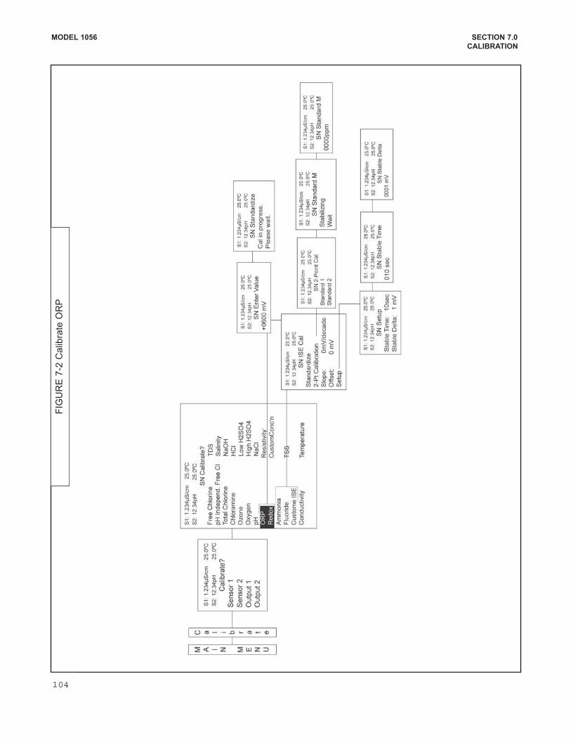
MODEL 1056 SECTION 7.0
CALIBRATION
FIG
UR
E 7
2 C
alib
rate
OR
P
104
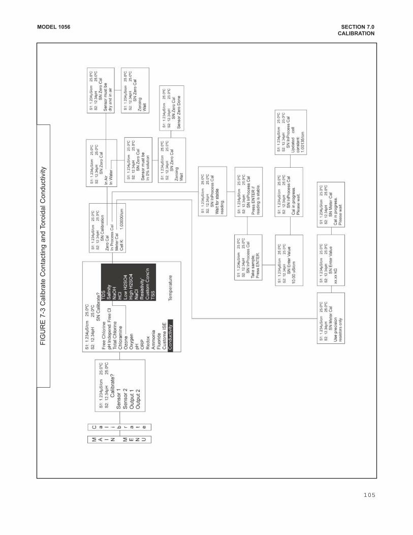
MODEL 1056 SECTION 7.0
CALIBRATION
FIG
UR
E 7
3 C
alib
rate
Conta
cting a
nd T
oro
idal C
ond
uctivity
105
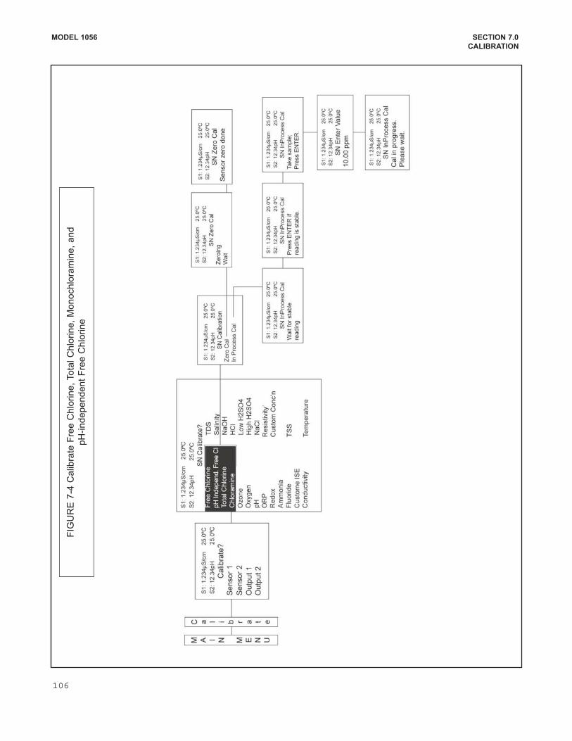
MODEL 1056 SECTION 7.0
CALIBRATION
FIG
UR
E 7
4 C
alib
rate
Fre
e C
hlo
rine,
Tota
l C
hlo
rine,
Monochlo
ram
ine,
and
pH
independent
Fre
e C
hlo
rine
106
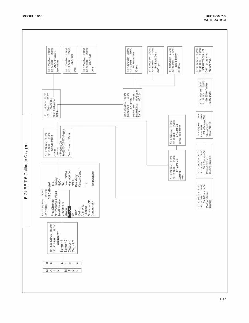
MODEL 1056 SECTION 7.0
CALIBRATION
FIG
UR
E 7
5 C
alib
rate
Oxygen
107
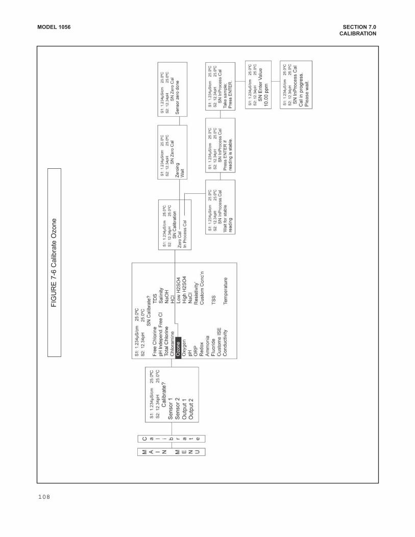
MODEL 1056 SECTION 7.0
CALIBRATION
FIG
UR
E 7
6 C
alib
rate
Ozone
108
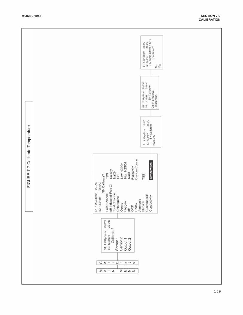
FIG
UR
E 7
7 C
alib
rate
Tem
pera
ture
MODEL 1056 SECTION 7.0
CALIBRATION
109
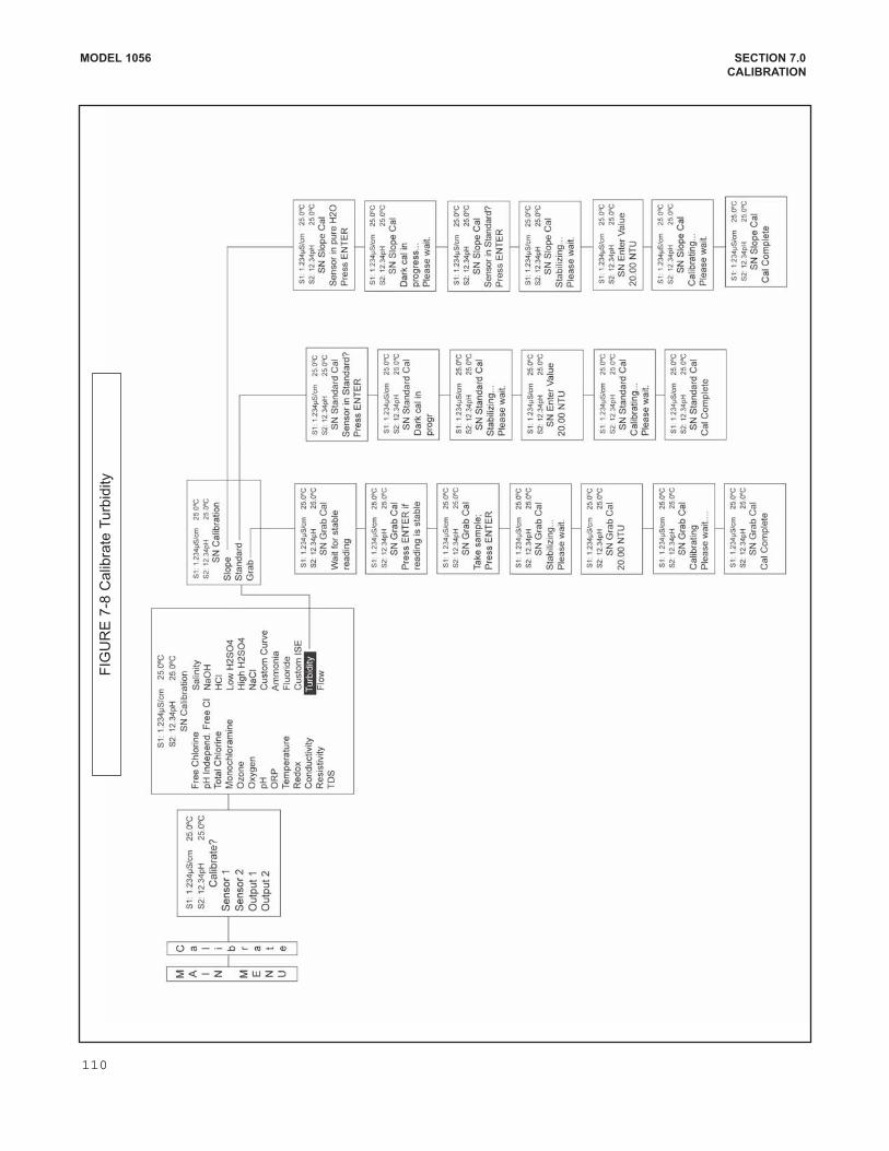
MODEL 1056 SECTION 7.0
CALIBRATION
FIG
UR
E 7
8 C
alib
rate
Turb
idity
110

MODEL 1056 SECTION 7.0
CALIBRATION
FIG
UR
E 7
9 C
alib
rate
Flo
w
111
SECTION 8.0
RETURN OF MATERIAL
17.1 GENERAL.
To expedite the repair and return of instruments, proper communication between the customer and the factory is
important. Before returning a product for repair, call 19497578500 for a Return Materials Authorization (RMA)
number.
17.2 WARRANTY REPAIR.
The following is the procedure for returning instruments still under warranty:
1. Call Rosemount Analytical for authorization.
2. To verify warranty, supply the factory sales order number or the original purchase order number. In the case
of individual parts or subassemblies, the serial number on the unit must be supplied.
3. Carefully package the materials and enclose your “Letter of Transmittal” (see Warranty). If possible, pack the
materials in the same manner as they were received.
4. Send the package prepaid to:
Emerson Process Management
Rosemount Analytical
2400 Barranca Parkway
Irvine, CA 92606
Attn: Factory Repair
RMA No. ____________
Mark the package: Returned for Repair
Model No. ____
17.3 NONWARRANTY REPAIR.
The following is the procedure for returning for repair instruments that are no longer under warranty:
1. Call Rosemount Analytical for authorization.
2. Supply the purchase order number, and make sure to provide the name and telephone number of the individ
ual to be contacted should additional information be needed.
3. Do Steps 3 and 4 of Section 17.2.
NOTE
Consult the factory for additional information regarding service or repair.
IMPORTANT
Please see second section of “Return of
Materials Request” form. Compliance with
the OSHA requirements is mandatory for
the safety of all personnel. MSDS forms
and a certification that the instruments have
been disinfected or detoxified are required.
MODEL 1056 SECTION 8.0
RETURN OF MATERIAL
112

A Worldwide Network of Sales and Service
Emerson Process Management’s field sales offices are your source for more information on the fill line of Rosemount Analyticalproducts. Field sales personnel will work closely with you to supply technical data and application information.
For more information, please contact your nearest Emerson Process Management sales office.
Immediate, Reliable Analytical Support Now there’s a way to quickly get the right answers for your liquid analytical instrumentation questions: the AnalyticalCustomer Support Center.
Our staff of trained professionals is ready to provide the information you need. If you are placing an order, verifying delivery,requesting application information, or just want to contact a Rosemount Analytical representative, a call to the CustomerSupport Center will provide you with the right people, the right answers, right now.
The right people, the right answers, right now.
THE AMERICAS HEADQUARTERS
Emerson Process Management
Rosemount Analytical Inc.
Liquid Center of Excellence
2400 Barranca Parkway
Irvine, CA 92606
Phone: +1.949.757.8500
Toll Free: +1.800.854.8257
Fax: +1.949.474.7250
ASIAPACIFIC
Emerson Process Management
Asia Pacific Private Ltd.
1 Pandan Crescent
Singapore 0512
Republic of Singapore
Phone: 65.777.8211
Fax: 65.777.0947
EUROPE
Emerson Process Management AG
Blegistrasse 21
CH6341 BaarWalterswil
Switzerland
T 41.41.768.6111
T 41.41.761.8740
VISIT OUR WEBSITE ATwww.rosemountanalytical.com
GERMANY
Emerson Process Management Process
Gas Analyzer Center of Excellence
GmbH & Co. OHG
Industriestrasse 1
63594 Hasselroth
Germany
T 49.6055.884.0
F 49.6055.884.20
LATIN AMERICA
Emerson Process Management
Rosemount Analytical
10241 West Little York, Suite #200
Houston, TX 77040 USA
T 713.467.6000
F 713.827.3328
MIDDLE EAST AND AFRICA
Emerson Process Management
EPM Building
P. O. Box 17033
Jebe Ali Free Zone
Dubai, United Arab Emirates
T 971.4.8835235
F 971.4.8835312
Credit Cards for U.S. Purchases Only.
The right people,the right answers,right now.
ONLINE ORDERING NOW AVAILABLE ON OUR WEB SITEhttp://www.rosemountanalytical.com
8
Emerson Process Management
2400 Barranca Parkway
Irvine, CA 92606 USA
Tel: (949) 7578500
Fax: (949) 4747250
http://www.rosemountanalytical.com
© Rosemount Analytical Inc. 2014