10.34: Numerical Methods Applied to Chemical Engineering · 10.34: Numerical Methods . Applied to...
35
10.34: Numerical Methods Applied to Chemical Engineering Finite Volume Methods Constructing Simulations of PDEs 1
Transcript of 10.34: Numerical Methods Applied to Chemical Engineering · 10.34: Numerical Methods . Applied to...

10.34: Numerical Methods Applied to
Chemical Engineering
Finite Volume MethodsConstructing Simulations of PDEs
1

Recap
• von Neumann stability analysis
• Finite volume methods
2

3
• Generally used for conservation equations of the form:
• is the density of a conserved quantity
• is the flux density of a conserved quantity
• The integral version of such an equation is:
Finite Volume Method
@b
@t= �r · j+ r(x, t)
b(x, t)
j(x, t)
d
dt
Z
V ⇤b(x, t) dV =
Z
S⇤n · j(x, t) dS +
Zr(x, t) dV
V ⇤
dB⇤(t) = F ⇤(t) +R⇤(t)
dtACC IN/OUT GEN/C
or
ON*

4
•
• What are each of these terms?
• B ⇤(t) = V ⇤b̄⇤(t)
• R ⇤(t) = V ⇤r̄⇤(t)
• F ⇤(t) =X
Fk(t) =k2faces⇤ k2
XA⇤
k(nk
•faces⇤
· j)(t)
the sum of fluxes through each face of the volume *db̄⇤
V ⇤ = Fk(t) + V ⇤r̄⇤(t)dt
• We want to solve for by approximating the reaction and flux terms. Let’s construct low order approximations physically.
dB⇤(t) = F ⇤(t) +R⇤(t)
dtACC IN/OUT GEN/CON
*
b̄(t)
X
k2faces⇤
Finite Volume MethodConservation within a finite volume:

5
*
@b=
@t�r · j+ r(x, t)
db̄⇤V ⇤ =
dtk2
XFk(t) + V ⇤r̄⇤(t)
faces⇤
Finite Volume Method

6
*
=@t
�r · j+ r(x, t)
db̄⇤V ⇤ =
dtk2
XFk(t) + V ⇤r̄⇤(t)
faces⇤
Finite Volume Method@b

7
@b=
@t�r · j+ r(x, t)
db̄⇤V ⇤ =
XFk(t) + V ⇤r̄⇤(t)
dt, France k2faces⇤
*
Geometrica: INRIA
Finite Volume Method
© INRIA. All rights reserved. This content is excluded from our Creative Commonslicense. For more information, see https://ocw.mit.edu/help/faq-fair-use/.

8
db̄⇤V ⇤ =
dtk2
XFk(t) + V ⇤r̄⇤(t)
faces⇤
*Cardiff et al. J Biomech Eng 136(1), 2013
Finite Volume Method@b
=@t
�r · j+ r(x, t)
© Cardiff, Philip et al. License: cc by-nc-nd. Some rights reserved. This content is excluded fromour CreativeCommons license. For more information, see https://ocw.mit.edu/help/faq-fair-use/.

9
Numerical Solution of PDEs
L
Step 1: domain decompositionfinite difference: nodes
i, j
W

10
Numerical Solution of PDEs
L
W
Step 1: domain decompositionfinite volume: cells
i, j

11L
W
Numerical Solution of PDEsStep 1: domain decomposition
finite element: elements (local basis functions)
i, j
12
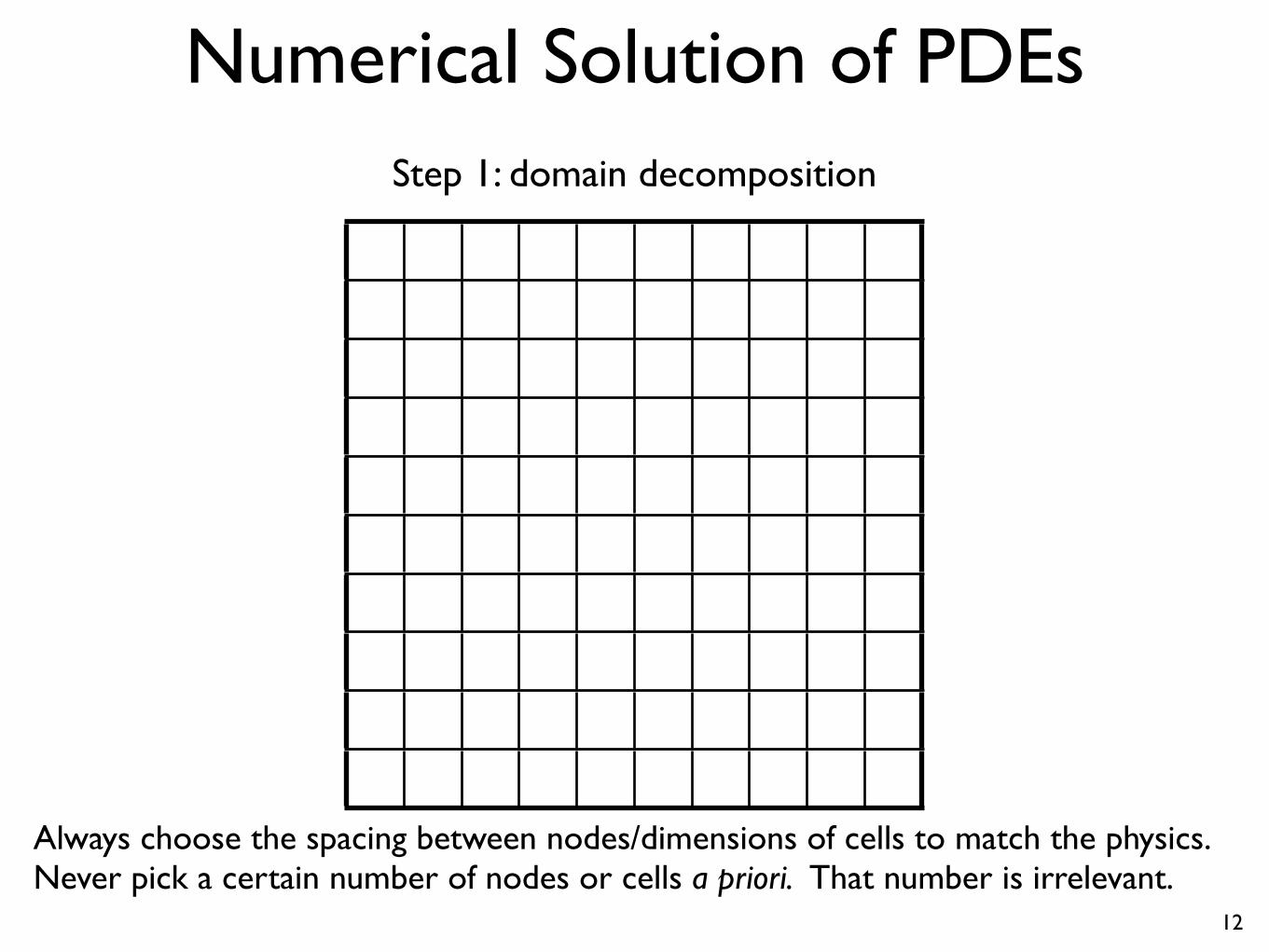
Numerical Solution of PDEsStep 1: domain decomposition
Always choose the spacing between nodes/dimensions of cells to match the physics. Never pick a certain number of nodes or cells a priori. That number is irrelevant.

13
19
x-coordinate (cm)
cm)
( etanidroco
y-
Concentration profile in (x,y)-space. Thin medical implant at x � [1,2] cm.
0 5 10 15 20 25 300
0.5
1
1.5
2
-2
0
2
4
6
8x 10⁻⁴
x-coordinate (cm)
y-co
ordi
nate
(cm
)
Close-up of concentration profile in (x,y)-space.
R =
30,
B =
2, N
= 3
00. S
emi-i
nfin
ite b
ound
ary
cond
ition
at x
=R a
nd y
=B: D
irich
let z
ero
conc
entra
tion.
0 2 4 6 8 100
0.02
0.04
0.06
0.08
0.1
-2
0
2
4
6
8x 10⁻⁴
Figure 6.2 Concentration profile using Dirichlet boundary condition for x = R and y = B. R = 30
cm, B = 2 cm, and N = 300.

14
Numerical Solution of PDEsStep 2: formulate an equation to be satisfied at each node/cell

15
Numerical Solution of PDEsStep 2: formulate an equation to be satisfied at each node/cellExample: at interior node/cell i,jr2c = 0
equation i,j: ci+1,j + ci�1,j + ci,j�1 + ci,j+1 � 4ci,j = 0
16
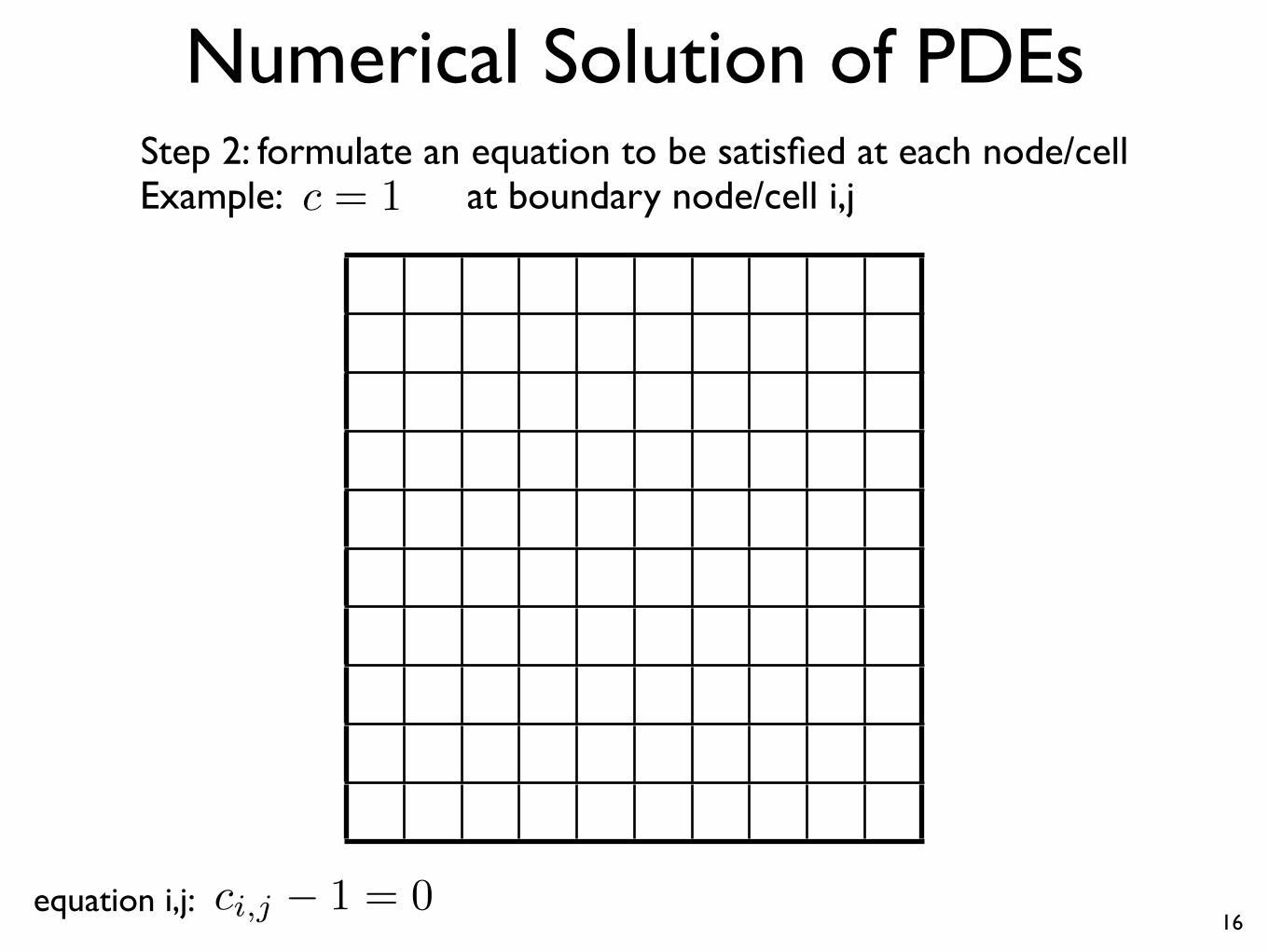
Numerical Solution of PDEsStep 2: formulate an equation to be satisfied at each node/cellExample: at boundary node/cell i,j
equation i,j:
c = 1
ci,j � 1 = 0

17
Numerical Solution of PDEsStep 3: solve the system of equations formulated at each node/cell for the
value of unknown function at each node/cell
f(c) = 0 If equations are linear, use linear iterative methodsIf equations are nonlinear, use nonlinear iterative methods

18
Numerical Solution of PDEsStep 3: solve the system of equations formulated at each node/cell for the
value of unknown function at each node/cell
f(c) = 0 must be a vector of the unknowns must be a vector of the equationscf

19
Numerical Solution of PDEs
1 Nx
Ny
1
2
i
j
Indexing
k = i+ (j � 1)Nx
ci,j+1 = ck+Nxck = ci,j or
k = j + (i� 1)Ny ci,j+1 = ck+1
3,

20
Numerical Solution of PDEs
y
1
, 2
i
j
Indexing
1 Nx
N
k = i+ (j � 1)Nxfk(c) = fi,j(c) or
k = j + (i� 1)Ny
3

21
Numerical Solution of PDEs
Ny
1
2
j
Indexing
1 Nx
k = i+ (j � 1)Nxfk(c) = fi,j(c) or
k = j + (i� 1)Ny
3,
i

22
Numerical Solution of PDEs
Nx
y
Nz
N
cl = ci,j,k, l =?
Exercise: write a single index for finite difference nodes in a cubic domain with (Nx, Ny, Nz) nodes in each cartesian direction

Numerical Solution of PDEsExercise: write a single index for finite difference nodes in a cubic
domain with (Nx, Ny, Nz) nodes in each cartesian direction
Nx
Ny
Nz
cl
= ci,j,k
, l = i+ (j � 1)Nx
+ (k � 1)Nx
Ny
23

Numerical Solution of PDEsExample: solve the diffusion equation in 2-D on a square with side = 1.
r2c = 0c = 0
c = 0
c = 0
c = 1
f(c) = 0
24

25
Numerical Solution of PDEsExample: solve the diffusion equation in 2-D on a square with side = 1.
h = 1 / 10; % Spacing between finite difference nodesNx = 1 + 1 / h; % Number of nodes in x-directionNy = Nx; % Number of nodes in y-direction
c0 = zeros( Nx * Ny, 1 ); % Initial guess for solution
c = fsolve( @( c ) my_func( c, Nx, Ny ), c0 ); % Find root of FD equations

26
Numerical Solution of PDEsExample: solve the diffusion equation in 2-D on a square with side = 1.
function f = my_func( c, Nx, Ny )
% Loop over all nodesfor i = 1:Nx
for j = 1:Ny
k = i + ( j - 1 ) * Nx; % Compound index
% Boundary nodesif ( i == 1 )
f( k ) = c( k );elseif ( i == Nx )
f( k ) = c( k );elseif( j == 1 )
f( k ) = c( k ) - 1;elseif( j == Ny )
f( k ) = c( k );
% Interior nodeselse
f( k ) = c( k + 1 ) + c( k - 1 ) + c( k - Nx ) + c( k + Nx ) - 4*c( k );end;
end;end;

27
Numerical Solution of PDEsExample: solve the diffusion equation in 2-D on a square with side = 1.
0 0.1 0.2 0.3 0.4 0.5 0.6 0.7 0.8 0.9 10
0.1
0.2
0.3
0.4
0.5
0.6
0.7
0.8
0.9
1
0.08 seconds to solve
h = 1/10
28
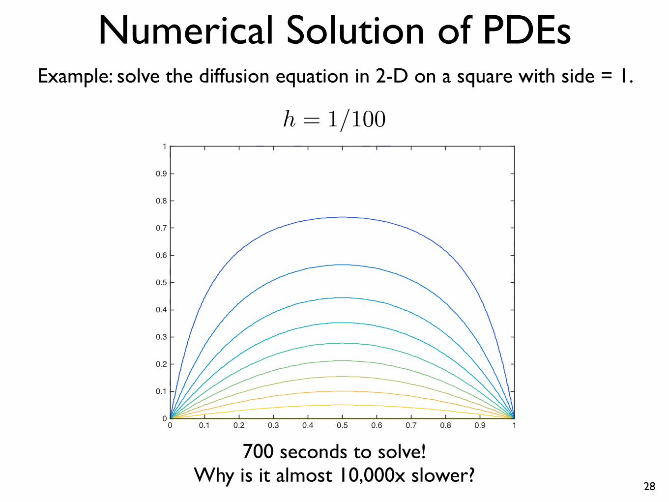
Numerical Solution of PDEsExample: solve the diffusion equation in 2-D on a square with side = 1.
0 0.1 0.2 0.3 0.4 0.5 0.6 0.7 0.8 0.9 10
0.1
0.2
0.3
0.4
0.5
0.6
0.7
0.8
0.9
1
h = 1/100
700 seconds to solve!Why is it almost 10,000x slower?

29
Numerical Solution of PDEsExample: solve the diffusion equation in 2-D on a square with side = 1.
f(c) = 0 = Ac� bfunction [ Ac, b ] = my_func( c, Nx, Ny )
Ac = sparse( Nx * Ny, 1 );b = sparse( Nx * Ny, 1 );
% Loop over all nodesfor i = 1:Nx
for j = 1:Ny
k = i + ( j - 1 ) * Nx; % Compound index
% Boundary nodesif ( i == 1 )
Ac( k ) = c( k );elseif ( i == Nx )
Ac( k ) = c( k );elseif( j == 1 )
Ac( k ) = c( k );b( k ) = 1;
elseif( j == Ny )Ac( k ) = c( k );
% Interior nodeselse
Ac( k ) = c( k + 1 ) + c( k - 1 ) + c( k - Nx ) + c( k + Nx ) - 4*c( k );end;
end;end;

30
Numerical Solution of PDEsExample: solve the diffusion equation in 2-D on a square with side = 1.
h = 1 / 10; % Spacing between finite difference nodesNx = 1 + 1 / h; % Number of nodes in x-directionNy = Nx; % Number of nodes in y-direction
% Calculate RHS of Ac = b[ Ac, b ] = my_func( zeros( Nx * Ny, 1 ), Nx, Ny );
% Find solution of linear FD equations using the an iterative method% This is gmres (generalized minimum residual). Other choices include % bicgstab (conjugate gradient), minres (minimum residual), etc.% The requires a function that returns A*c given c.c = gmres( @( c ) my_func( c, Nx, Ny ), b, 100, 1e-6, 100 );

31
Numerical Solution of PDEsExample: solve the diffusion equation in 2-D on a square with side = 1.
0.015 seconds to solve!
0 0.1 0.2 0.3 0.4 0.5 0.6 0.7 0.8 0.9 10
0.1
0.2
0.3
0.4
0.5
0.6
0.7
0.8
0.9
1h = 1/10

32
Numerical Solution of PDEsExample: solve the diffusion equation in 2-D on a square with side = 1.
5 seconds to solve!
0 0.1 0.2 0.3 0.4 0.5 0.6 0.7 0.8 0.9 10
0.1
0.2
0.3
0.4
0.5
0.6
0.7
0.8
0.9
1h = 1/100

33
Numerical Solution of PDEsExample: solve the diffusion equation in 2-D on a square with side = 1.
function [ Ac, b ] = my_func( c, Nx, Ny )
Ac = sparse( Nx * Ny, 1 );b = sparse( Nx * Ny, 1 ); k = i+ (j � 1)N
x
% Define indices of boundary points and interior points bottom = [ 1:Nx ]; top = Nx*Ny - [ 1:Nx ]; left = [ 1:Nx:Nx*Ny ]; right = [ Nx:Nx:Nx*Ny ]; interior = setdiff( [ 1:Nx*Ny ], [ left, right, bottom, top ] );
Ac( left ) = c( left );Ac( right ) = c( right );Ac( top ) = c( top );Ac( bottom ) = c( bottom );b( bottom ) = 1;
A( interior ) = c( interior - 1 ) + c( interior + 1 ) + c( interior - Nx ) + c( interior + Nx ) …- 4 * c( interior );
f(c) = 0 = Ac� b

34
Numerical Solution of PDEsExample: solve the diffusion equation in 2-D on a square with side = 1.
1.2 seconds to solve!
0 0.1 0.2 0.3 0.4 0.5 0.6 0.7 0.8 0.9 10
0.1
0.2
0.3
0.4
0.5
0.6
0.7
0.8
0.9
1h = 1/100

MIT OpenCourseWarehttps://ocw.mit.edu
10.34 Numerical Methods Applied to Chemical EngineeringFall 2015
For information about citing these materials or our Terms of Use, visit: https://ocw.mit.edu/terms.