10.1.1.157.5222(1)

ACTIVE CONTROL OF SURGE IN CENTRIFUGAL COMPRESSORS USING

MAGNETIC TIP CLEARANCE ACTUATION

A Dissertation

Presented to

the Faculty of the School of Engineering and Applied Science

University of Virginia

In Partial Fulfillment

of the Requirements for the Degree of

Doctor of Philosophy in Mechanical and Aerospace Engineering

by

Dorsa Sanadgol

August 2006

APPROVAL SHEET

This dissertation is submitted in partial fulfillment of the requirements for the degree of

Doctor of Philosophy in Mechanical and Aerospace Engineering

Dorsa Sanadgol

This dissertation has been read and approved by the Examining Committee:

Professor Eric H. Maslen, Dissertation Advisor

Professor Zongli Lin

Professor Hossein Haj-Hariri

Professor Tetsuya Iwasaki

Professor Carl Knospe

Accepted for the School of Engineering and Applied Science:

Dean, School of Engineering and Applied Science

August 2006

ABSTRACT

One of the major operational problems of centrifugal compressors is the occurrence

of surge. This flow instability degrades the performance of the compressor and limits its

stable operating range. The most common surge protection mechanism is flow recycling. A

recycling valve opens if the operating point of the machine gets close to a predicted surge

point to prevent further reduction in flow. This causes a considerable waste and energy,

specifically, when the valve has to respond to sudden changes in the flow which usually

results in a great deal of overshooting in the recycled flow.

This research presents a new method for active surge control in centrifugal compres-

sors with unshrouded impellers using a magnetic thrust bearing to modulate the impeller

tip clearance. Magnetic bearings offer the potential for active control of flow instabilities.

This capability is highly dependent on the sensitivity of the compressor characteristics to

blade tip clearance. If the position of the shaft can be actuated with sufficient authority

and speed, the induced pressure modulation makes control of surge promising. The active

nature of the magnetic bearing system makes the real–time static and dynamic positioning

of the rotor and therefore modulation of the impeller tip clearance possible.

A theoretical model is first established that describes the sensitivity of the centrifu-

gal compressor characteristic curve to tip clearance variations induced by axial motion of

the rotor. The impeller is assumed to be unshrouded, generally enhancing this sensitivity.

Using the known effects of static changes in the tip clearance on compressor parameters, a

one dimensional incompressible flow model is developed to predict the effects of dynamic

tip clearance variations. The developed model for the effects of tip clearance modulation

on the centrifugal compressor characteristics curve parameters is used to develop a surge

control method by modulating the impeller tip clearance using a magnetic thrust bearing.

First, the existing model for the dynamics of the compression system is extended to include

the influence of dynamic tip clearance modulation. A nonlinear controller is then devel-

oped using the backstepping methods with the objective that system trajectories remain on

the steady state compressor characteristic curve. This ensures zero steady state offset of

the impeller, which maintains the performance and efficiency of the compressor. Effects of

sudden changes downstream of the compressor are modeled as uncertainties in the throttle

setting and are included in the control synthesis. To take the dynamic limitations of the

actuator into account, the dynamics of the thrust bearing is also included in the design of

the nonlinear controller.

Results from simulation of the nonlinear model for a single stage high-speed cen-

trifugal compressor show that using the proposed control method, mass flow and pressure

oscillations associated with compressor surge are quickly suppressed with acceptable tip

clearance excursions, typically less than 20% of the available clearance. It is shown that

it is possible to produce adequate axial excursions in the clearance between the impeller

blades and the adjacent stationary shroud using a magnetic thrust bearing with practical

levels of drive voltage.

This surge control method would allow centrifugal compressors to reliably and

safely operate with a wider range than is currently done in the field. The principal ad-

vantage of the proposed approach over conventional surge control methods lies in that,

in machines already equipped with magnetic bearing, the method can potentially be imple-

mented by simply modifying controller software. This dispenses with the need to introduce

additional hardware, permitting adaptation of existing machinery at virtually no cost. In ad-

dition, since the controller is designed with the objective of keeping the trajectories on the

compressor characteristic curve, the compressor performance and efficiency are no longer

sacrificed by excessive recycling to achieve stability.

In order to explore these conjectures experimentally, a high speed centrifugal com-

pressor test facility with active magnetic bearings is developed. The test facility can be

used for implementing the proposed surge control method and also for assessing the im-

peller and bearing loads at off–design conditions. This data can then be used to verify

and refine analytical models used in compressor design. Magnetic levitation of the rotor

is established in radial and axial directions. A PID controller is used for the levitation of

the radial bearings. An H∞ controller with reference tracking is used for controlling the

magnetic thrust bearing. The controllers are successfully implemented on the test rig.

ACKNOWLEDGMENTS

I would most like to thank my advisor Professor Eric Maslen for his inspirations,

encouragement and guidance throughout my studies, and for giving me the opportunity to

work on this exciting project. I am very grateful for his support and friendship.

Special thanks and appreciation to Professor Zongli Lin for his support and in-

terest in this project, Professor Hossein Haj-Hariri for his advice on developing the fluid

dynamic model, Professor Carl Knospe for his constructive criticism and scrutinizing ques-

tions that made me think beyond the surface of problems, and Professor Tetsuya Iwasaki

for always being available to give advice on control problems and giving the most amazing

and insightful lectures on controls. I would also like to thank visiting post doctorate fellow

Hyeong-Joon Ahn for his help and advice on developing the tip clearance model.

I greatly appreciate the financial support of the ROMAC Laboratories and also the

help and advice of the ROMAC faculty and students. I am very grateful to the KOBE Steel

company for their generous support, especially to Mr. Koichiro Iizuka and Mr. Toshikazu

Miyaji for their help and their interest in this research.

I wish to thank Professor George Gillies for his encouragement and always having

what I was looking for, and Wei Jiang for his electronic wizardry. I would also like to

acknowledge the support of the staff of the Mechanical and Aerospace Engineering De-

partment: Jerry O’Leary for his computer support, Lewis Steva, Kevin Knight and Claude

Mitchell for their continuous machine shop support over the years, Ed Spencely from the

Aerospace Research Laboratory for helping with the rotor repair and having all the tools

that I needed, and Brittany Rugo for her friendship and knowing the answers to all my

administrative questions.

I owe a debt of gratitude to former graduate students: Nathan Brown and Eric

Buskirk. It has been a great pleasure working with them. I have learned a lot from them,

especially about tropical fish from Eric Buskirk. I wish to thank Qing Yu (flofish) Wang

for his help in the early stages of my studies. I would also like to thank the two bright

undergraduate students who participated in this project: James Chiu for always being ready

to help and his work on developing the motor cooling system and Danielle Christensen for

developing the instrumentation system and great squash games.

I would like to thank Hunter Cloud for his friendship, and his help and advice with

the experimental work, Karen Marshall for being a true friend, and always being there

for me, Bahar Sharafi for listening to my complaints and all the wonderful time that we

spent together, Mehdi Shafieian for preparing the best Persian food while he was in Char-

lottesville and sending me my favorite Persian food even when he moved to Philadelphia,

and Ali Nezamoddini for always coming up with something to cheer me up and his great

dinners.

No word can describe my appreciation for the love, support and encouragement of

my parents, sister and brother throughout the years and during my stay away from them. I

am truly blessed to have them. Finally, I am most grateful for the love and support of my

wonderful husband Matthias Glauser. I could have never done it without his friendship,

love, patience, encouragement, help and support.

vi

CONTENTS

ABSTRACT . . . . . . . . . . . . . . . . . . . . . . . . . . . . . . . . . . . . . . . i

ACKNOWLEDGMENTS . . . . . . . . . . . . . . . . . . . . . . . . . . . . . . . . iv

LIST OF ILLUSTRATIONS . . . . . . . . . . . . . . . . . . . . . . . . . . . . . . xi

LIST OF TABLES . . . . . . . . . . . . . . . . . . . . . . . . . . . . . . . . . . . xviii

Chapter

1. INTRODUCTION AND PROBLEM STATEMENT . . . . . . . . . . . . . . 1

1.1. Flow Instabilities in Compressors . . . . . . . . . . . . . . . . . . . 1

1.1.1. Rotating Stall . . . . . . . . . . . . . . . . . . . . . . . . 1

1.1.2. Surge . . . . . . . . . . . . . . . . . . . . . . . . . . . . . 4

1.2. Surge Protection . . . . . . . . . . . . . . . . . . . . . . . . . . . . 7

1.2.1. Surge Avoidance . . . . . . . . . . . . . . . . . . . . . . . 9

1.2.2. Active Control . . . . . . . . . . . . . . . . . . . . . . . . 11

1.3. Modeling . . . . . . . . . . . . . . . . . . . . . . . . . . . . . . . . 13

1.4. Research Objective . . . . . . . . . . . . . . . . . . . . . . . . . . . 14

1.5. Problem Statement . . . . . . . . . . . . . . . . . . . . . . . . . . . 15

1.6. Thesis Statement . . . . . . . . . . . . . . . . . . . . . . . . . . . . 16

1.7. Innovative Aspects and Impact of Work . . . . . . . . . . . . . . . . 17

1.8. Dissertation Outline . . . . . . . . . . . . . . . . . . . . . . . . . . . 18

2. MODELING THE COMPRESSION SYSTEM . . . . . . . . . . . . . . . . . 19

2.1. Compressor and Throttle Characteristics . . . . . . . . . . . . . . . . 20

2.1.1. Nondimensionalization . . . . . . . . . . . . . . . . . . . 23

2.2. Greitzer Compression System Model . . . . . . . . . . . . . . . . . . 24

2.2.1. Surge Simulation for the Current Compressor . . . . . . . 27

2.3. Tip Clearance Effects . . . . . . . . . . . . . . . . . . . . . . . . . . 29

2.4. Compressor Model with Tip Clearance Effects . . . . . . . . . . . . . 33

2.5. Model Linearization . . . . . . . . . . . . . . . . . . . . . . . . . . 37

2.6. Quasi-Static Assumption . . . . . . . . . . . . . . . . . . . . . . . . 42

2.7. Model Uncertainties . . . . . . . . . . . . . . . . . . . . . . . . . . 43

2.8. Model Validation . . . . . . . . . . . . . . . . . . . . . . . . . . . . 44

2.9. Summary . . . . . . . . . . . . . . . . . . . . . . . . . . . . . . . . 47

3. ACTIVE CONTROL OF SURGE . . . . . . . . . . . . . . . . . . . . . . . . 48

3.1. Model . . . . . . . . . . . . . . . . . . . . . . . . . . . . . . . . . . 49

3.2. Stabilization with Mass Flow Feedback . . . . . . . . . . . . . . . . 51

3.2.1. Simulation Results . . . . . . . . . . . . . . . . . . . . . . 53

3.3. Sliding Mode Control . . . . . . . . . . . . . . . . . . . . . . . . . . 60

3.4. Sliding Mode for Surge Control . . . . . . . . . . . . . . . . . . . . 63

3.5. Integrator Backstepping . . . . . . . . . . . . . . . . . . . . . . . . . 64

3.6. Backstepping for Surge Control . . . . . . . . . . . . . . . . . . . . 66


3.7. Thrust Bearing Dynamics . . . . . . . . . . . . . . . . . . . . . . . . 70

3.8. Backstepping with Chain of Integrators for Active Control of Surge . 71


3.9. Bandwidth Limitations . . . . . . . . . . . . . . . . . . . . . . . . . 80

3.10.Stabilization with Uncertainties . . . . . . . . . . . . . . . . . . . . . 83

3.11.Backstepping with Uncertainties . . . . . . . . . . . . . . . . . . . . 87


3.12.Backstepping with Uncertainties and Bandwidth Limitations . . . . . 95

3.13.Conclusion . . . . . . . . . . . . . . . . . . . . . . . . . . . . . . . 96

4. EXPERIMENTAL FACILITY AND SYSTEM IDENTIFICATION . . . . . . 99

4.1. Test Rig Overview . . . . . . . . . . . . . . . . . . . . . . . . . . . 99

4.1.1. Compressor . . . . . . . . . . . . . . . . . . . . . . . . . 101

4.1.2. Test Section . . . . . . . . . . . . . . . . . . . . . . . . . 102

4.1.3. Motor . . . . . . . . . . . . . . . . . . . . . . . . . . . . 109

4.1.4. Coupling and Alignment . . . . . . . . . . . . . . . . . . 110

4.1.5. Ducting System . . . . . . . . . . . . . . . . . . . . . . . 113

4.1.6. Data Acquisition System . . . . . . . . . . . . . . . . . . 115

4.2. Rotor Identification . . . . . . . . . . . . . . . . . . . . . . . . . . . 115

4.2.1. Impact Test . . . . . . . . . . . . . . . . . . . . . . . . . 115

4.2.2. Theoretical Critical Speeds Map . . . . . . . . . . . . . . 121

4.3. Radial Bearings Identification . . . . . . . . . . . . . . . . . . . . . 123

4.3.1. Radial Position Sensors . . . . . . . . . . . . . . . . . . . 124

4.3.2. Force per Current Coefficient, k i . . . . . . . . . . . . . . 127

4.3.3. Open-Loop Stiffness, kx . . . . . . . . . . . . . . . . . . . 133

4.4. Thrust Bearing Identification . . . . . . . . . . . . . . . . . . . . . . 134

4.4.1. Axial Position Sensors . . . . . . . . . . . . . . . . . . . . 135

4.4.2. Force per Current Coefficient, k i . . . . . . . . . . . . . . 137

4.4.3. Open-Loop Stiffness, kx . . . . . . . . . . . . . . . . . . . 140

4.5. Amplifier Identification . . . . . . . . . . . . . . . . . . . . . . . . . 142

4.6. Summary . . . . . . . . . . . . . . . . . . . . . . . . . . . . . . . . 144

5. MAGNETIC LEVITATION . . . . . . . . . . . . . . . . . . . . . . . . . . . 145

5.1. Magnetic Bearing Overview . . . . . . . . . . . . . . . . . . . . . . 145

5.2. Control Computer . . . . . . . . . . . . . . . . . . . . . . . . . . . . 146

5.2.1. RTLinux Operating System . . . . . . . . . . . . . . . . . 147

5.2.2. Control Software . . . . . . . . . . . . . . . . . . . . . . . 151

5.3. Thrust Bearing Controller . . . . . . . . . . . . . . . . . . . . . . . . 151

5.3.1. Thrust Bearing Model . . . . . . . . . . . . . . . . . . . . 152

5.3.2. PID Controller for Thrust Bearing . . . . . . . . . . . . . . 156

5.3.3. H∞ Controller for Thrust Bearing . . . . . . . . . . . . . 156

5.3.4. H∞ Controller with Reference Tracking . . . . . . . . . . 163

5.4. Radial Bearing Controller . . . . . . . . . . . . . . . . . . . . . . . . 171

5.5. Conclusion . . . . . . . . . . . . . . . . . . . . . . . . . . . . . . . 174

6. CONCLUSION AND FUTURE RESEARCH . . . . . . . . . . . . . . . . . . 175

6.1. Conclusion of the Analytical Work . . . . . . . . . . . . . . . . . . . 176

6.2. Conclusion of the Experimental Work . . . . . . . . . . . . . . . . . 180

6.3. Future Research . . . . . . . . . . . . . . . . . . . . . . . . . . . . . 181

APPENDIX

A. BACKSTEPPING CALCULATIONS . . . . . . . . . . . . . . . . . . . . . . 183

A.1. Backstepping with Chain of Integrators . . . . . . . . . . . . . . . . 184

A.2. Backstepping with Uncertainties . . . . . . . . . . . . . . . . . . . . 191

B. VARIABLE FREQUENCY DRIVE SETTINGS . . . . . . . . . . . . . . . . 193

C. AMPLIFIER MANUAL . . . . . . . . . . . . . . . . . . . . . . . . . . . . . 195

D. INSTRUCTIONS TO OPERATE THE CONTROLLER . . . . . . . . . . . . 200

E. INSTRUCTIONS FOR COMMISSIONING THE TEST RIG . . . . . . . . . 203

REFERENCES . . . . . . . . . . . . . . . . . . . . . . . . . . . . . . . . . . . . . 205

xi

ILLUSTRATIONS

Figure Page

1.1. Rotating stall inception mechanism . . . . . . . . . . . . . . . . . . . . . . . 2

1.2. Types of rotating stall [11] . . . . . . . . . . . . . . . . . . . . . . . . . . . . 3

1.3. Different rotating stall characteristics [11] . . . . . . . . . . . . . . . . . . . . 4

1.4. Schematic of the surge cycle . . . . . . . . . . . . . . . . . . . . . . . . . . . 5

1.5. Typical frequency range of rotating stall and surge [23] . . . . . . . . . . . . . 6

1.6. Deep surge cycle [22] . . . . . . . . . . . . . . . . . . . . . . . . . . . . . . 7

1.7. Blade damage due to surge, Copyright 2002 AVICOMP CONTROLS . . . . . 8

1.8. Damage to an Elliott 90P centrifugal compressor due to surge . . . . . . . . . 8

1.9. Bleed effect on the compressor characteristic map [12] . . . . . . . . . . . . . 9

1.10. Typical compressor characteristic map with surge avoidance line [12] . . . . . 10

1.11. Typical anti-surge system - CCI DRAG . . . . . . . . . . . . . . . . . . . . . 11

2.1. Compression system schematic . . . . . . . . . . . . . . . . . . . . . . . . . 20

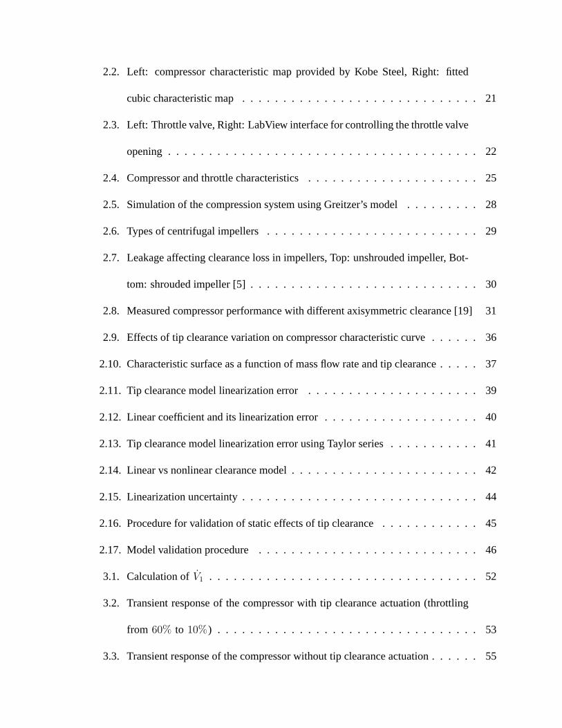
2.2. Left: compressor characteristic map provided by Kobe Steel, Right: fitted

cubic characteristic map . . . . . . . . . . . . . . . . . . . . . . . . . . . . . 21

2.3. Left: Throttle valve, Right: LabView interface for controlling the throttle valve

opening . . . . . . . . . . . . . . . . . . . . . . . . . . . . . . . . . . . . . . 22

2.4. Compressor and throttle characteristics . . . . . . . . . . . . . . . . . . . . . 25

2.5. Simulation of the compression system using Greitzer’s model . . . . . . . . . 28

2.6. Types of centrifugal impellers . . . . . . . . . . . . . . . . . . . . . . . . . . 29

2.7. Leakage affecting clearance loss in impellers, Top: unshrouded impeller, Bot-

tom: shrouded impeller [5] . . . . . . . . . . . . . . . . . . . . . . . . . . . . 30

2.8. Measured compressor performance with different axisymmetric clearance [19] 31

2.9. Effects of tip clearance variation on compressor characteristic curve . . . . . . 36

2.10. Characteristic surface as a function of mass flow rate and tip clearance . . . . . 37

2.11. Tip clearance model linearization error . . . . . . . . . . . . . . . . . . . . . 39

2.12. Linear coefficient and its linearization error . . . . . . . . . . . . . . . . . . . 40

2.13. Tip clearance model linearization error using Taylor series . . . . . . . . . . . 41

2.14. Linear vs nonlinear clearance model . . . . . . . . . . . . . . . . . . . . . . . 42

2.15. Linearization uncertainty . . . . . . . . . . . . . . . . . . . . . . . . . . . . . 44

2.16. Procedure for validation of static effects of tip clearance . . . . . . . . . . . . 45

2.17. Model validation procedure . . . . . . . . . . . . . . . . . . . . . . . . . . . 46

3.1. Calculation of V1 . . . . . . . . . . . . . . . . . . . . . . . . . . . . . . . . . 52

3.2. Transient response of the compressor with tip clearance actuation (throttling

from 60% to 10%) . . . . . . . . . . . . . . . . . . . . . . . . . . . . . . . . 53

3.3. Transient response of the compressor without tip clearance actuation . . . . . . 55

3.4. Transient response of the compressor with tip clearance actuation (throttling

from 60% to 10% and back to 60%) . . . . . . . . . . . . . . . . . . . . . . 56

3.5. Block diagram of the control system with mass flow feedback - thrust bearing

modeled as a low pass filter . . . . . . . . . . . . . . . . . . . . . . . . . . . 57

3.6. Transient response of the compressor with the thrust bearing modeled as a low

pass filter . . . . . . . . . . . . . . . . . . . . . . . . . . . . . . . . . . . . . 58

3.7. Bandwidth demand from the thrust bearing . . . . . . . . . . . . . . . . . . . 59

3.8. Transient response of the compressor with tip clearance actuation using back-

stepping method . . . . . . . . . . . . . . . . . . . . . . . . . . . . . . . . . 70

3.9. Transient response and control requirement for backstepping with chain of

integrators . . . . . . . . . . . . . . . . . . . . . . . . . . . . . . . . . . . . 78

3.10. Detail of Fig. 3.9-f, input voltage to the thrust bearing . . . . . . . . . . . . . 79

3.11. Transient response and control requirement for step change in the throttle setting 81

3.12. Block diagram of the controller . . . . . . . . . . . . . . . . . . . . . . . . . 83

3.13. Bandwidth requirement for backstepping surge controller . . . . . . . . . . . . 84

3.14. Transient response and control requirement for backstepping with uncertainties 91

3.15. Transient response and control requirement for backstepping with uncertain-

ties - integral action added to compensate for steady state offset . . . . . . . . 93

3.16. Transient response and control requirement for step change in the throttle set-

ting - backstepping with uncertainties . . . . . . . . . . . . . . . . . . . . . . 94

3.17. Transient response for backstepping with uncertainties - thrust bearing mod-

eled as a low pass filter . . . . . . . . . . . . . . . . . . . . . . . . . . . . . . 96

4.1. Assembly of the compressor test facility . . . . . . . . . . . . . . . . . . . . . 100

4.2. Left: impeller, Right: volute . . . . . . . . . . . . . . . . . . . . . . . . . . . 101

4.3. Pressure sensor placement . . . . . . . . . . . . . . . . . . . . . . . . . . . . 102

4.4. Top: bare rotor, Bottom: final rotor assembly with lamination stacks and iso-

lation rings . . . . . . . . . . . . . . . . . . . . . . . . . . . . . . . . . . . . 103

4.5. Geometry of the E-core radial magnetic actuator . . . . . . . . . . . . . . . . 104

4.6. Left: motor side radial magnetic bearing, Right: compressor side radial mag-

netic bearing . . . . . . . . . . . . . . . . . . . . . . . . . . . . . . . . . . . 105

4.7. Lamination stacks for radial bearings and radial position sensors . . . . . . . . 106

4.8. Flux path of the magnetic thrust bearing [6] . . . . . . . . . . . . . . . . . . . 107

4.9. Left and middle: thrust stators, Right: thrust stator with windings . . . . . . . 107

4.10. Left: compressor side backup bearing, Right: motor side backup bearing . . . 108

4.11. Motor installed on the baseplate and the variable frequency drive . . . . . . . . 109

4.12. Machinery damage caused by excessive misalignment [3] . . . . . . . . . . . 111

4.13. Schematic of the Rim and Face method [40] . . . . . . . . . . . . . . . . . . . 113

4.14. Left: shaft hubs, Right: Rim and Face indicator setup for aligning the shafts . . 113

4.15. Layout of the piping arrangement . . . . . . . . . . . . . . . . . . . . . . . . 114

4.16. Data acquisition user interface . . . . . . . . . . . . . . . . . . . . . . . . . . 116

4.17. Rotor suspended on piano wires to approximate the free-free support . . . . . 117

4.18. Set up for impact testing . . . . . . . . . . . . . . . . . . . . . . . . . . . . . 118

4.19. Impact test measurement for identifying the first bending mode . . . . . . . . 119

4.20. Different rotor configurations for impact testing . . . . . . . . . . . . . . . . . 120

4.21. Impact test measurement for identifying the diaphragm mode . . . . . . . . . 120

4.22. Critical speed map . . . . . . . . . . . . . . . . . . . . . . . . . . . . . . . . 122

4.23. Mode shapes . . . . . . . . . . . . . . . . . . . . . . . . . . . . . . . . . . . 123

4.24. SKF magnetic radial bearing and the variable reluctance sensors assembly . . . 124

4.25. Initial calibration of the reluctance sensors . . . . . . . . . . . . . . . . . . . 125

4.26. Sensor conditioning box, Top: circuit diagram, Bottom: hardware . . . . . . . 127

4.27. Bandwidth of the sensor conditioning box . . . . . . . . . . . . . . . . . . . . 128

4.28. Calibration of the reluctance sensors . . . . . . . . . . . . . . . . . . . . . . . 128

4.29. Sensors sign convention . . . . . . . . . . . . . . . . . . . . . . . . . . . . . 129

4.30. Load cell calibration . . . . . . . . . . . . . . . . . . . . . . . . . . . . . . . 130

4.31. Force calculation at motor side bearing . . . . . . . . . . . . . . . . . . . . . 130

4.32. Measurement of ki in x direction for the motor side radial bearing . . . . . . . 131

4.33. Measurement of ki in y direction for the motor side radial bearing . . . . . . . 131

4.34. Force calculation at compressor side bearing . . . . . . . . . . . . . . . . . . 132

4.35. Measurement of ki in x direction for the compressor side radial bearing . . . . 133

4.36. Measurement of ki in y direction for the compressor side radial bearing . . . . 133

4.37. Force generated from control current as the rotor moves in x direction . . . . . 135

4.38. Force generated from control current as the rotor moves in y direction . . . . . 136

4.39. Eddy current sensor . . . . . . . . . . . . . . . . . . . . . . . . . . . . . . . . 136

4.40. Target for the eddy current sensors . . . . . . . . . . . . . . . . . . . . . . . . 137

4.41. Eddy current sensor sensitivity . . . . . . . . . . . . . . . . . . . . . . . . . . 137

4.42. Measurement of ki for the thrust bearing . . . . . . . . . . . . . . . . . . . . 138

4.43. Measurement of kx for the thrust bearing . . . . . . . . . . . . . . . . . . . . 140

4.44. Measured and modeled transfer function of the amplifier . . . . . . . . . . . . 144

5.1. Schematic of a magnetic bearing system . . . . . . . . . . . . . . . . . . . . . 146

5.2. System block diagram . . . . . . . . . . . . . . . . . . . . . . . . . . . . . . 147

5.3. Details of the bare Linux kernel [18] . . . . . . . . . . . . . . . . . . . . . . . 149

5.4. Real-time task scheduling . . . . . . . . . . . . . . . . . . . . . . . . . . . . 150

5.5. Detail of the RTLinux kernel [18] . . . . . . . . . . . . . . . . . . . . . . . . 150

5.6. Control software . . . . . . . . . . . . . . . . . . . . . . . . . . . . . . . . . 152

5.7. Simple thrust bearing model . . . . . . . . . . . . . . . . . . . . . . . . . . . 153

5.8. Thrust bearing model from Zhu [51] . . . . . . . . . . . . . . . . . . . . . . . 154

5.9. Thrust bearing model comparison . . . . . . . . . . . . . . . . . . . . . . . . 155

5.10. Measured closed loop transfer function of the reference position to tracking

error with PID controller . . . . . . . . . . . . . . . . . . . . . . . . . . . . . 157

5.11. System block diagram . . . . . . . . . . . . . . . . . . . . . . . . . . . . . . 158

5.12. Detailed system block diagram . . . . . . . . . . . . . . . . . . . . . . . . . . 158

5.13. Bode plots of the sensors(Gs ), analog filter(Gf ), and Pade approximation(Gp )

transfer functions . . . . . . . . . . . . . . . . . . . . . . . . . . . . . . . . . 160

5.14. Plant realization for H∞ control design . . . . . . . . . . . . . . . . . . . . . 163

5.15. Attempt to introduce integral control in H∞ . . . . . . . . . . . . . . . . . . . 164

5.16. H∞ controller with integrator block diagram . . . . . . . . . . . . . . . . . . 165

5.17. Plant realization for H∞ control design with reference tracking . . . . . . . . 168

5.18. Transfer functions for the different weighting functions . . . . . . . . . . . . . 169

5.19. Controller transfer function [Non dimensional] . . . . . . . . . . . . . . . . . 169

5.20. H∞ performance . . . . . . . . . . . . . . . . . . . . . . . . . . . . . . . . . 170

5.21. Measured closed loop transfer function of the H∞ controller . . . . . . . . . . 171

5.22. Comparison between closed loop performance of PID and H∞ controllers . . 171

5.23. PID controller transfer function for motor side and compressor side radial

bearings . . . . . . . . . . . . . . . . . . . . . . . . . . . . . . . . . . . . . . 173

5.24. PID controller design for radial bearings . . . . . . . . . . . . . . . . . . . . . 173

5.25. Measured rotor position and bearing currents with the levitation controller run-

ning: PID for the radial bearings and H∞ for the thrust bearing . . . . . . . . 174

C.1. Calibration of amplifier #1, Left: current monitor gain, Right: amplifier gain . 196










xviii

TABLES

Table Page

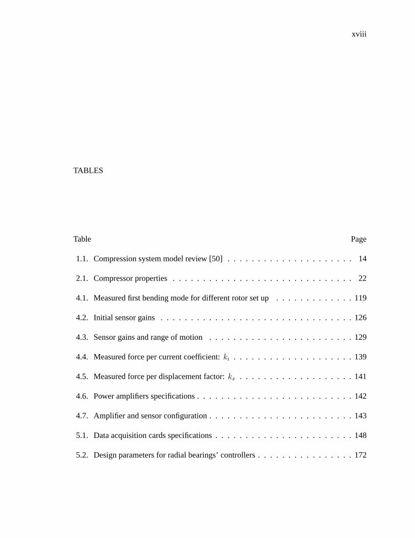
1.1. Compression system model review [50] . . . . . . . . . . . . . . . . . . . . . 14

2.1. Compressor properties . . . . . . . . . . . . . . . . . . . . . . . . . . . . . . 22

4.1. Measured first bending mode for different rotor set up . . . . . . . . . . . . . 119

4.2. Initial sensor gains . . . . . . . . . . . . . . . . . . . . . . . . . . . . . . . . 126

4.3. Sensor gains and range of motion . . . . . . . . . . . . . . . . . . . . . . . . 129

4.4. Measured force per current coefficient: ki . . . . . . . . . . . . . . . . . . . . 139

4.5. Measured force per displacement factor: kx . . . . . . . . . . . . . . . . . . . 141

4.6. Power amplifiers specifications . . . . . . . . . . . . . . . . . . . . . . . . . . 142

4.7. Amplifier and sensor configuration . . . . . . . . . . . . . . . . . . . . . . . . 143

5.1. Data acquisition cards specifications . . . . . . . . . . . . . . . . . . . . . . . 148

5.2. Design parameters for radial bearings’ controllers . . . . . . . . . . . . . . . . 172

1

CHAPTER 1

INTRODUCTION AND PROBLEM STATEMENT

1.1 Flow Instabilities in Compressors

The stable operating range of compressors is limited at low mass flow rates by

surge, rotating stall or a combination of both. Rotating stall and surge have been a problem

for compressors as long as these machines have existed. No matter which one of these flow

instabilities occur, it has detrimental effects on the system and must be avoided.

1.1.1 Rotating Stall

Generally in stall, flow is separated from its path walls. Rotating stall is a localized

flow instability where one or more regions of stall cells (stagnant flow) rotate around the

circumference of the compressor at a constant speed, which is a fraction of the rotating

2

speed of the rotor, usually between twenty and seventy percent of the rotor speed. The

average flow is steady and does not vary with time but the flow is circumferentially nonuni-

form. There is insignificant net through-flow in the stall cells. The mechanism of stall

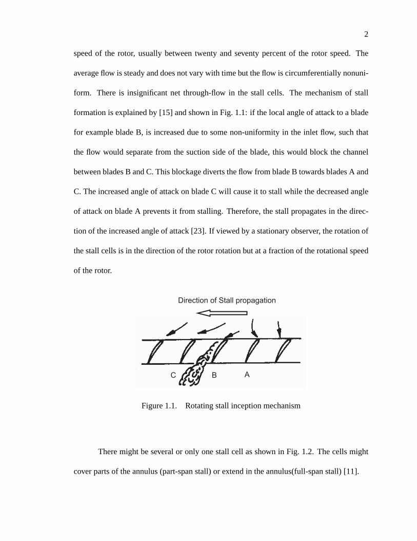
formation is explained by [15] and shown in Fig. 1.1: if the local angle of attack to a blade

for example blade B, is increased due to some non-uniformity in the inlet flow, such that

the flow would separate from the suction side of the blade, this would block the channel

between blades B and C. This blockage diverts the flow from blade B towards blades A and

C. The increased angle of attack on blade C will cause it to stall while the decreased angle

of attack on blade A prevents it from stalling. Therefore, the stall propagates in the direc-

tion of the increased angle of attack [23]. If viewed by a stationary observer, the rotation of

the stall cells is in the direction of the rotor rotation but at a fraction of the rotational speed

of the rotor.

Direction of Stall propagation

ABC

Figure 1.1. Rotating stall inception mechanism

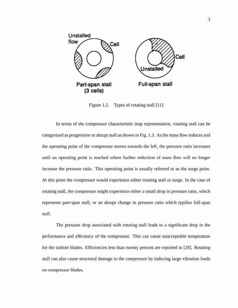
There might be several or only one stall cell as shown in Fig. 1.2. The cells might

cover parts of the annulus (part-span stall) or extend in the annulus(full-span stall) [11].

3

Figure 1.2. Types of rotating stall [11]

In terms of the compressor characteristic map representation, rotating stall can be

categorized as progressive or abrupt stall as shown in Fig. 1.3. As the mass flow reduces and

the operating point of the compressor moves towards the left, the pressure ratio increases

until an operating point is reached where further reduction of mass flow will no longer

increase the pressure ratio. This operating point is usually referred to as the surge point.

At this point the compressor would experience either rotating stall or surge. In the case of

rotating stall, the compressor might experience either a small drop in pressure ratio, which

represents part-span stall; or an abrupt change in pressure ratio which typifies full-span

stall.

The pressure drop associated with rotating stall leads to a significant drop in the

performance and efficiency of the compressor. This can cause unacceptable temperature

for the turbine blades. Efficiencies less than twenty percent are reported in [28]. Rotating

stall can also cause structural damage to the compressor by inducing large vibration loads

on compressor blades.

4

Figure 1.3. Different rotating stall characteristics [11]

Rotating stall is a major concern in axial compressors. Whether rotating stall plays

an important role in the performance of centrifugal compressors is still an issue of debate

in the compressor community. However, de Jagger [12] and Emmons [15] have shown that

rotating stall has a negligible effect on the performance of centrifugal compressors. The

centrifugal compressor’s tolerance to stall is believed to come from the fact that much of

the impeller pressure rise is produced by centrifugal effects which will occur even in the

presence of rotating stall [11]. Therefore, the main concern for these machines is surge.

1.1.2 Surge

The major operational problem for centrifugal compressors is the occurrence of

surge. This flow instability degrades the performance of the compressor and limits its sta-

ble operating range: fully developed surge is very destructive and must be meticulously

avoided. Surge is a flow instability that affects the whole compression system and is char-

acterized by large oscillations in the pressure rise and mass flow rate. During surge, flow

5

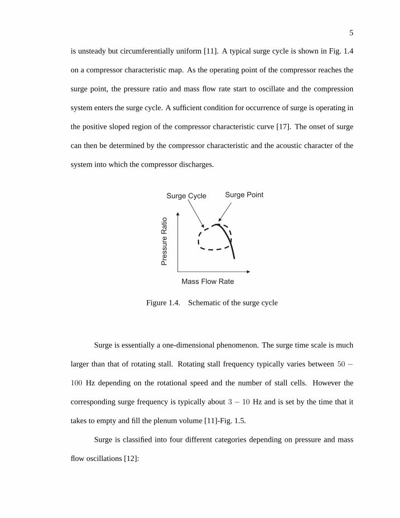
is unsteady but circumferentially uniform [11]. A typical surge cycle is shown in Fig. 1.4

on a compressor characteristic map. As the operating point of the compressor reaches the

surge point, the pressure ratio and mass flow rate start to oscillate and the compression

system enters the surge cycle. A sufficient condition for occurrence of surge is operating in

the positive sloped region of the compressor characteristic curve [17]. The onset of surge

can then be determined by the compressor characteristic and the acoustic character of the

system into which the compressor discharges.

Mass Flow Rate

Pre

ssur

e R

atio

Surge PointSurge Cycle

Figure 1.4. Schematic of the surge cycle

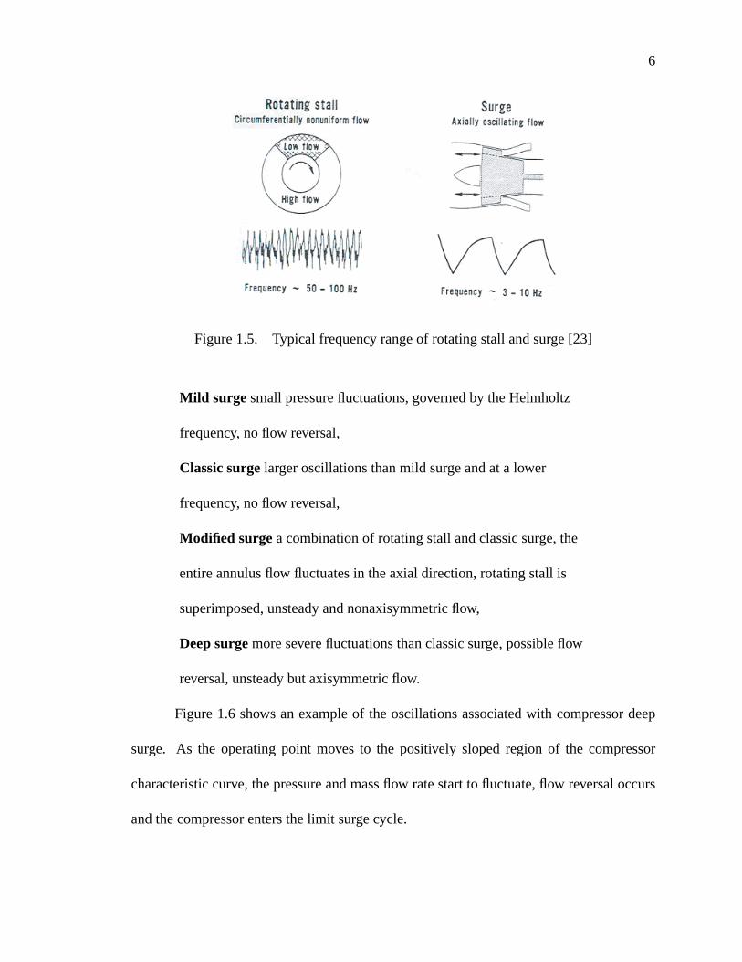
Surge is essentially a one-dimensional phenomenon. The surge time scale is much

larger than that of rotating stall. Rotating stall frequency typically varies between 50 −

100 Hz depending on the rotational speed and the number of stall cells. However the

corresponding surge frequency is typically about 3 − 10 Hz and is set by the time that it

takes to empty and fill the plenum volume [11]-Fig. 1.5.

Surge is classified into four different categories depending on pressure and mass

flow oscillations [12]:

6

Figure 1.5. Typical frequency range of rotating stall and surge [23]

Mild surge small pressure fluctuations, governed by the Helmholtz

frequency, no flow reversal,

Classic surge larger oscillations than mild surge and at a lower

frequency, no flow reversal,

Modified surge a combination of rotating stall and classic surge, the

entire annulus flow fluctuates in the axial direction, rotating stall is

superimposed, unsteady and nonaxisymmetric flow,

Deep surge more severe fluctuations than classic surge, possible flow

reversal, unsteady but axisymmetric flow.

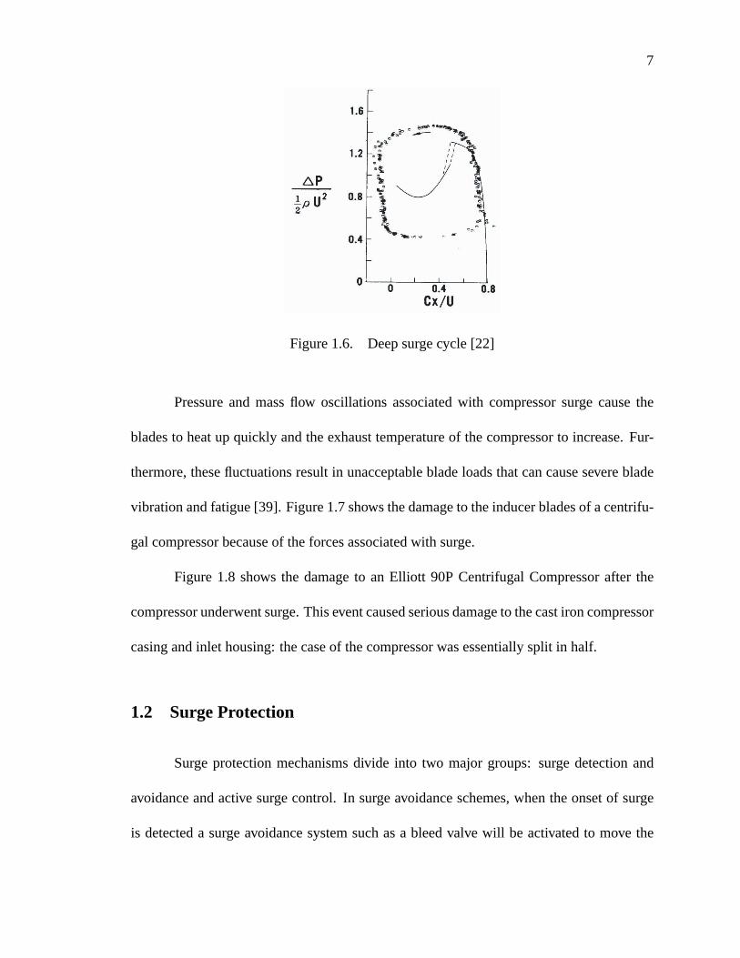
Figure 1.6 shows an example of the oscillations associated with compressor deep

surge. As the operating point moves to the positively sloped region of the compressor

characteristic curve, the pressure and mass flow rate start to fluctuate, flow reversal occurs

and the compressor enters the limit surge cycle.

7

Figure 1.6. Deep surge cycle [22]

Pressure and mass flow oscillations associated with compressor surge cause the

blades to heat up quickly and the exhaust temperature of the compressor to increase. Fur-

thermore, these fluctuations result in unacceptable blade loads that can cause severe blade

vibration and fatigue [39]. Figure 1.7 shows the damage to the inducer blades of a centrifu-

gal compressor because of the forces associated with surge.

Figure 1.8 shows the damage to an Elliott 90P Centrifugal Compressor after the

compressor underwent surge. This event caused serious damage to the cast iron compressor

casing and inlet housing: the case of the compressor was essentially split in half.

1.2 Surge Protection

Surge protection mechanisms divide into two major groups: surge detection and

avoidance and active surge control. In surge avoidance schemes, when the onset of surge

is detected a surge avoidance system such as a bleed valve will be activated to move the

8

Figure 1.7. Blade damage due to surge, Copyright 2002 AVICOMP CONTROLS

Figure 1.8. Damage to an Elliott 90P centrifugal compressor due to surge

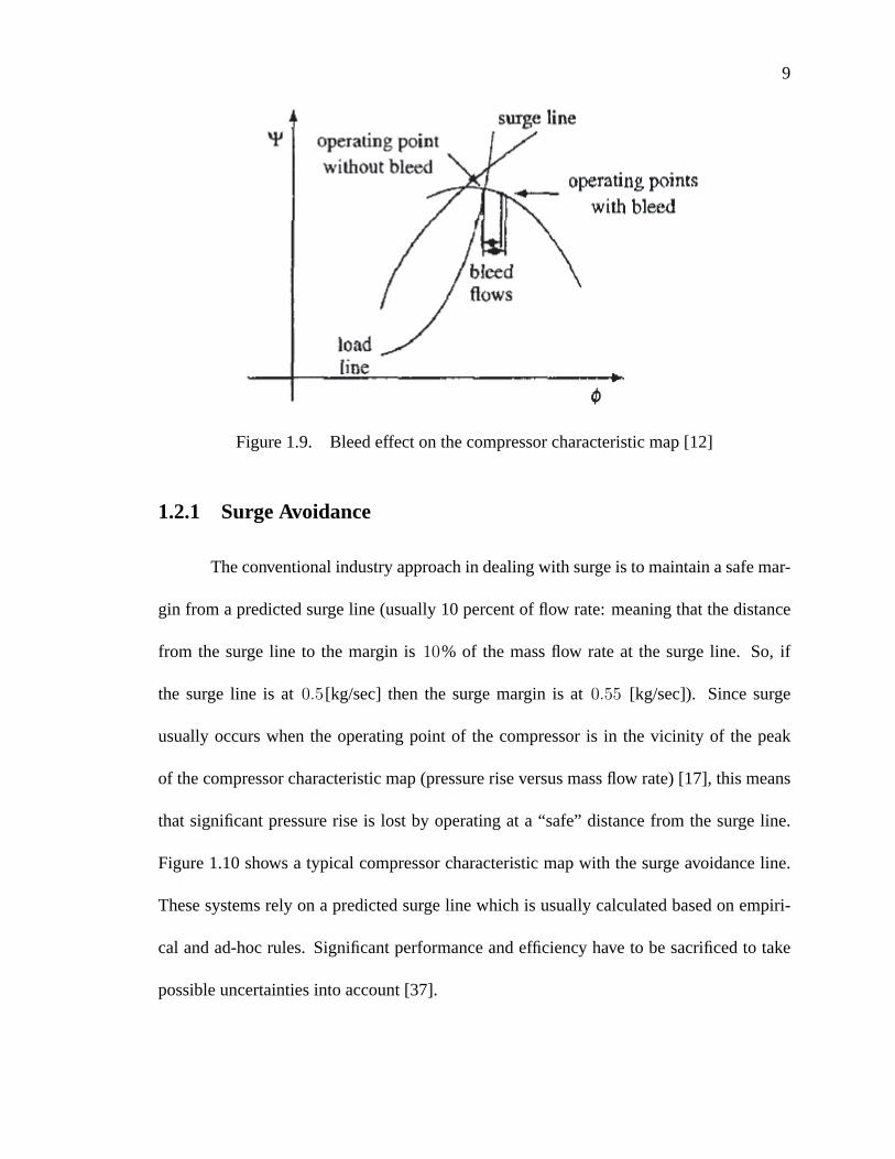
operating point of the system to a point away from the surge line, Fig. 1.9. In the active

surge control system, the compression system parameters are constantly monitored by vari-

ous sensors, a controller provides the required signal to actuators that will influence system

parameters and stabilize the operating point.

9

Figure 1.9. Bleed effect on the compressor characteristic map [12]

1.2.1 Surge Avoidance

The conventional industry approach in dealing with surge is to maintain a safe mar-

gin from a predicted surge line (usually 10 percent of flow rate: meaning that the distance

from the surge line to the margin is 10% of the mass flow rate at the surge line. So, if

the surge line is at 0.5[kg/sec] then the surge margin is at 0.55 [kg/sec]). Since surge

usually occurs when the operating point of the compressor is in the vicinity of the peak

of the compressor characteristic map (pressure rise versus mass flow rate) [17], this means

that significant pressure rise is lost by operating at a “safe” distance from the surge line.

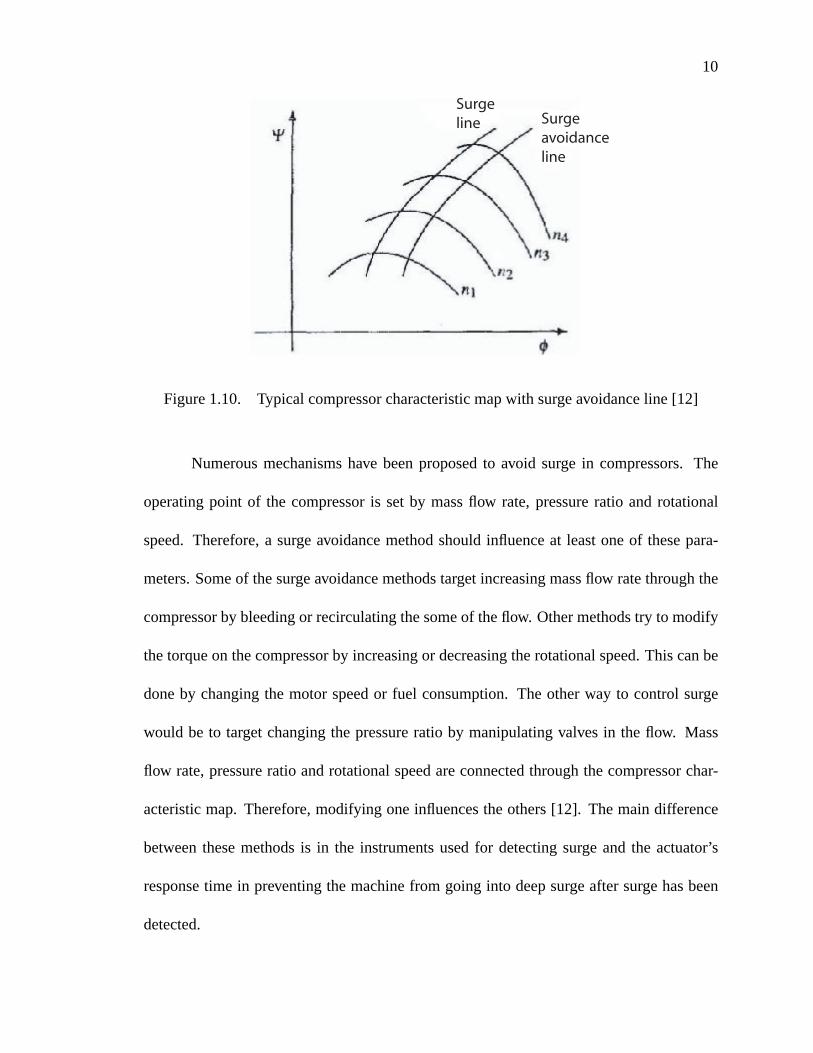
Figure 1.10 shows a typical compressor characteristic map with the surge avoidance line.

These systems rely on a predicted surge line which is usually calculated based on empiri-

cal and ad-hoc rules. Significant performance and efficiency have to be sacrificed to take

possible uncertainties into account [37].

10

Surgeline Surge

avoidanceline

Figure 1.10. Typical compressor characteristic map with surge avoidance line [12]

Numerous mechanisms have been proposed to avoid surge in compressors. The

operating point of the compressor is set by mass flow rate, pressure ratio and rotational

speed. Therefore, a surge avoidance method should influence at least one of these para-

meters. Some of the surge avoidance methods target increasing mass flow rate through the

compressor by bleeding or recirculating the some of the flow. Other methods try to modify

the torque on the compressor by increasing or decreasing the rotational speed. This can be

done by changing the motor speed or fuel consumption. The other way to control surge

would be to target changing the pressure ratio by manipulating valves in the flow. Mass

flow rate, pressure ratio and rotational speed are connected through the compressor char-

acteristic map. Therefore, modifying one influences the others [12]. The main difference

between these methods is in the instruments used for detecting surge and the actuator’s

response time in preventing the machine from going into deep surge after surge has been

detected.

11

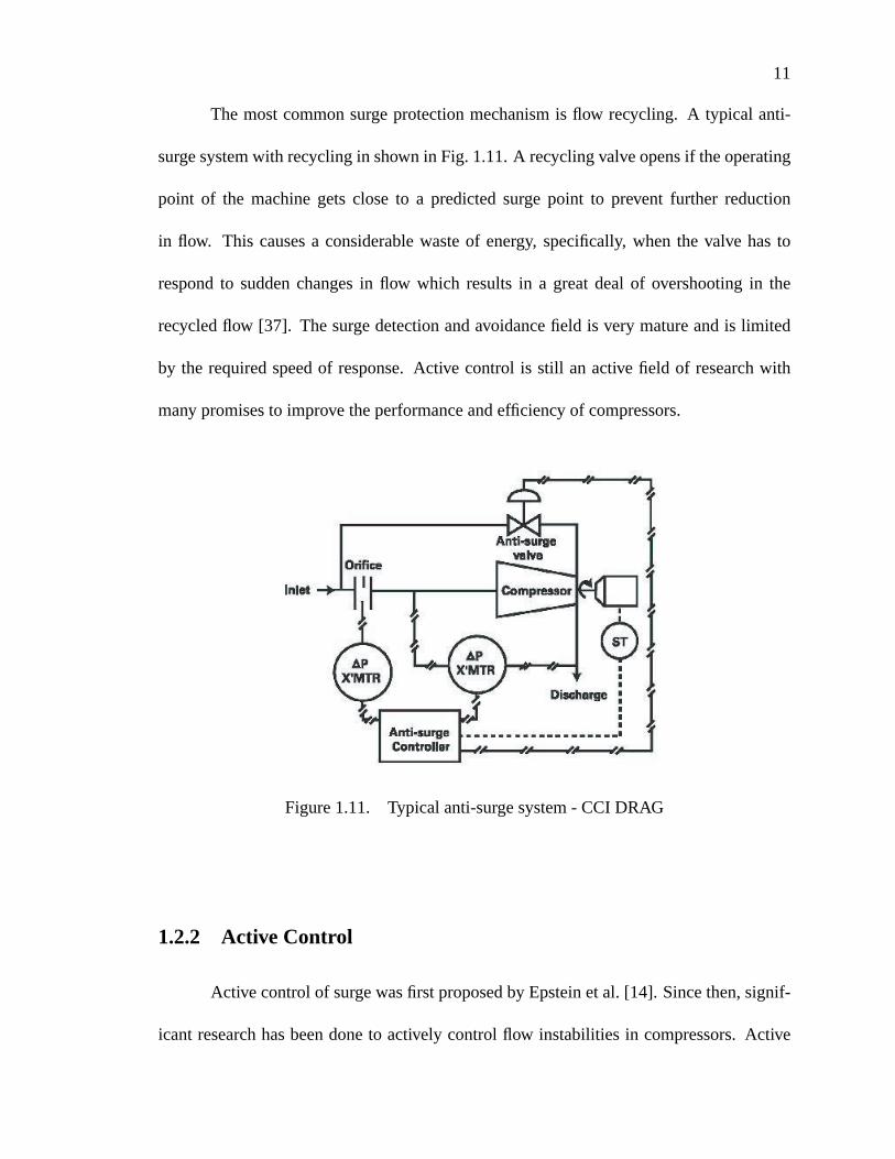
The most common surge protection mechanism is flow recycling. A typical anti-

surge system with recycling in shown in Fig. 1.11. A recycling valve opens if the operating

point of the machine gets close to a predicted surge point to prevent further reduction

in flow. This causes a considerable waste of energy, specifically, when the valve has to

respond to sudden changes in flow which results in a great deal of overshooting in the

recycled flow [37]. The surge detection and avoidance field is very mature and is limited

by the required speed of response. Active control is still an active field of research with

many promises to improve the performance and efficiency of compressors.

Figure 1.11. Typical anti-surge system - CCI DRAG

1.2.2 Active Control

Active control of surge was first proposed by Epstein et al. [14]. Since then, signif-

icant research has been done to actively control flow instabilities in compressors. Active

12

control of surge could help reducing the down time related to maintenance of equipment

because of surge and could also improve the efficiency and reliability of compression sys-

tems. Since surge is a one dimensional instability, a one dimensional actuator can be used

to control it. Actuators such as valves [39], a movable wall [25], or a loud speaker [16] have

been used in the literature. Typical sensors used in the active surge control are pressure and

mass flow sensors.

Despite many successful attempts to extend the stable operating range of the com-

pressor using active control mechanisms [4, 16], there has not been a general solution. Most

of the approaches require extensive knowledge about the system, only work on a specific

machine and do not take possible disturbances upstream or downstream of the compressor

into consideration in the design of the controller. Information about how the control system

reacts in the presence of these disturbances is necessary in setting the correct surge margin

for the compressor and would help the user in choosing a machine with a wider range of

operation.

Another area of improvement in active surge control is in the type of the controller

that is used to design the active control system. Using advanced control methods such as

nonlinear or adaptive control can extend the stable operating range of the compressor. To

summarize, the points of investigations in active surge control are:

1. type and number of sensors used for detecting flow conditions,

2. type and number of actuators used to control surge,

3. Type of the controller that is used in the control synthesis [12].

13

The need to improve the current practice in centrifugal compressor surge control

has become apparent to operating companies, and was confirmed by an industry survey

conducted by GMRC [37] in 2000.

1.3 Modeling

A mathematical model that is able to predict the onset of surge/rotating stall and the

dynamics of the compression system while the compressor is operating in surge/rotating

stall is necessary to design an active surge/rotating stall controller. Considerable research

has been done in deriving reliable models for the compression system behavior’s in the

presence of surge or rotating stall. The first extensive work in the area of modeling com-

pressor instabilities was done by Greitzer [22]. Greitzer’s model was originally developed

for low speed axial compressors. Hansen et al. [26] successfully adapted Greitzer’s model

to a small centrifugal compressor. Fink et al [17] showed that Greitzer’s model can be

applied to predict surge in a turbocharger and also included the effects of rotor speed varia-

tions in the Greitzer’s model. Others have done similar work to produce more complicated

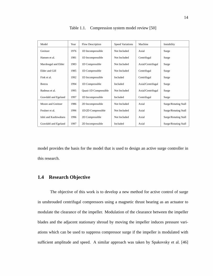
models that would also include the compressibility effects. Table 1.1 provides an overview

of the available models in the literature.

Even though compressor surge is a complicated phenomenon, it is essentially a one

dimensional nonlinear instability and can be described using a one dimensional nonlinear

model. The Greitzer model has been successfully applied to several centrifugal compres-

sors [20, 39, 50] and also used for active surge control purposes [20, 39, 50]. Greitzer’s

14

Table 1.1. Compression system model review [50]

Model Year Flow Description Speed Variations Machine Instability

Greitzer 1976 1D Incompressible Not Included Axial Surge

Hansen et al. 1981 1D Incompressible Not Included Centrifugal Surge

Macdougal and Elder 1983 1D Compressible Not Included Axial/Centrifugal Surge

Elder and Gill 1985 1D Compressible Not Included Centrifugal Surge

Fink et al. 1992 1D Incompressible Included Centrifugal Surge

Botros 1994 1D Compressible Included Axial/Centrifugal Surge

Badmus et al. 1995 Quasi-1D Compressible Not Included Axial/Centrifugal Surge

Gravdahl and Egeland 1997 1D Incompressible Included Centrifugal Surge

Moore and Greitzer 1986 2D Incompressible Not Included Axial Surge/Rotating Stall

Feulner et al. 1996 1D/2D Compressible Not Included Axial Surge/Rotating Stall

Ishii and Kashiwabara 1996 2D Compressible Not Included Axial Surge/Rotating Stall

Gravdahl and Egeland 1997 2D Incompressible Included Axial Surge/Rotating Stall

model provides the basis for the model that is used to design an active surge controller in

this research.

1.4 Research Objective

The objective of this work is to develop a new method for active control of surge

in unshrouded centrifugal compressors using a magnetic thrust bearing as an actuator to

modulate the clearance of the impeller. Modulation of the clearance between the impeller

blades and the adjacent stationary shroud by moving the impeller induces pressure vari-

ations which can be used to suppress compressor surge if the impeller is modulated with

sufficient amplitude and speed. A similar approach was taken by Spakovsky et al. [46]

15

to control rotating stall in axial compressors using radial modulations of the rotor with

magnetic radial bearings. Use of axial motion in centrifugal compressors to control surge,

distinguishes this work from that of Spakovsky et al. [46]. They were able to reduce the

stalling mass flow rate by 2.3 percent using radial modulation of the rotor in an axial com-

pressor. Comparable results were obtained by Weigl et al. [49] using unsteady air injection

in the same compressor which showed that tip clearance modulations can significantly con-

tribute to flow stabilization.

The effect of passive tip clearance control on surge has been studied by [13]. Eisen-

lohr and Chladek [13] looked at increasing tip clearance to shift the surge line to lower mass

flow rates. A larger clearance, however, is accompanied by a reduced efficiency. The major

advantage of the approach taken in the current research over the one implemented in [13]

is that the blade tip clearance is actively modulated with a magnetic thrust bearing, but the

mean tip clearance is kept at the design value. This way the performance and efficiency of

the compressor is not sacrificed to control surge.

1.5 Problem Statement

To make a commercially viable surge control system using magnetic thrust bearing

actuation, the following hypotheses should be examined:

1. It is possible to exert a useful level of control authority over the dynamics of com-

pressor surge in unshrouded centrifugal compressors by modulating the impeller

tip clearance.

16

2. It is possible to design a feedback controller based on mass flow rate and pressure

rise that stabilizes the compressor surge even in the presence of suitably bounded

downstream pressure or throttle disturbances.

3. These state variables can be adequately estimated from practical pressure measure-

ments.

4. It is possible to produce adequate axial excursions using a physically feasible mag-

netic thrust bearing with practical levels of drive voltage.

1.6 Thesis Statement

The primary goal of this research is to develop a theoretical basis that addresses

hypotheses 1, 2, and 4 above by pursuing the following:

1. Develop a model for the effects of tip clearance modulation on the centrifugal

compressor characteristics curve parameters.

2. Extend existing models for the dynamics of the compression system (compres-

sor - plenum volume - throttle) to include the influence of dynamic tip clearance

modulation.

3. Develop a method for active control of surge in centrifugal compressors using tip

clearance modulation with a magnetic thrust bearing in the presence of disturbance

downstream of the compressor.

4. Establish the bandwidth requirement of such a controller considering the limita-

tions of conventional magnetic thrust bearings and correlate it to the size of toler-

ated disturbances.

17

Design and commissioning of a test rig that would allow for: 1) conducting experi-

ments to investigate the validity of the derived model and 2) implementing an active surge

control system, is another major part of this work.

1.7 Innovative Aspects and Impact of Work

The advantage that this method provides over the conventional surge control meth-

ods is that no additional hardware need be added to the system if the machine is already

equipped with magnetic bearings. The only modification would be in the thrust bearing

control algorithm, thereby minimizing the cost of surge mitigation. In addition, since the

controller is designed with the objective of keeping the trajectories on the compressor char-

acteristic curve, the compressor performance and efficiency are no longer sacrificed by

excessive recycling to achieve stability. This surge control method would allow centrifugal

compressors to reliably and safely operate with a wider range than is currently done in the

field in the presence of disturbances, would eliminate the wasted energy due to excessive

recycling and is robust to downstream pressure and throttle disturbances.

Furthermore, when this test rig is commissioned, it will provide a test bench to

determine the bearing loads and the aerodynamic cross couplings at off design conditions

using magnetic bearings as load cells. At the design point, the bearing loads due to aerody-

namic flows are zero but at other operating points, they can be substantial. There are some

design guidelines available for estimating off-design loading but they often produce very

poor estimates. This is a problem because resizing bearings after the compressor design is

complete is very difficult. Consequently, the evolution of compressor designs is slow and

18

very conservative. Such data could be used to calibrate existing models or to validate CFD

based predictions. Better predictive tools would permit more aggressive design and would,

hopefully, contribute to substantially better performance across the technology.

1.8 Dissertation Outline

Developing a model for the compression system that includes the effects of tip

clearance actuation is discussed in Chapter 2. A new method for active control of surge in

unshrouded centrifugal compressors using magnetic thrust bearing actuation is developed

and presented in Chapter 3. The development of an experimental test facility that would

allow for conducting experiments to validate the tip clearance model and the proposed

surge control method is discussed in Chapter 4. Designing the levitating controllers for the

magnetic bearings is explained in Chapter 5. Conclusions and future research suggestions

are summarized in Chapter 6.

19

CHAPTER 2

MODELING THE COMPRESSION SYSTEM

A mathematical model that is capable of predicting surge and describing flow dy-

namics during compressor surge is needed in order to design a surge controller. The well

established Greitzer compressor model is used to model the compression system. A mathe-

matical model is derived that describes the effects of tip clearance modulation on the com-

pressor characteristic curve. This model is integrated with the Greitzer model to provide a

model for the compression system that provides authority over the blade tip clearance and

can further be used to design a surge controller using tip clearance actuation.

20

2.1 Compressor and Throttle Characteristics

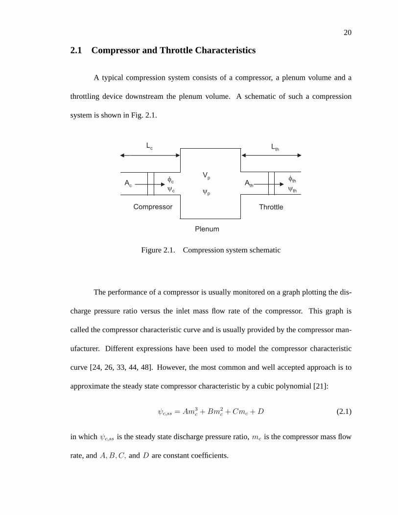
A typical compression system consists of a compressor, a plenum volume and a

throttling device downstream the plenum volume. A schematic of such a compression

system is shown in Fig. 2.1.

ψp

Vp

ψthψc

Throttle

Plenum

Compressor

Lc

Ac

Lth

Athφc φth

Figure 2.1. Compression system schematic

The performance of a compressor is usually monitored on a graph plotting the dis-

charge pressure ratio versus the inlet mass flow rate of the compressor. This graph is

called the compressor characteristic curve and is usually provided by the compressor man-

ufacturer. Different expressions have been used to model the compressor characteristic

curve [24, 26, 33, 44, 48]. However, the most common and well accepted approach is to

approximate the steady state compressor characteristic by a cubic polynomial [21]:

ψc,ss = Am3c +Bm2

c + Cmc +D (2.1)

in which ψc,ss is the steady state discharge pressure ratio, mc is the compressor mass flow

rate, and A,B,C, and D are constant coefficients.

21

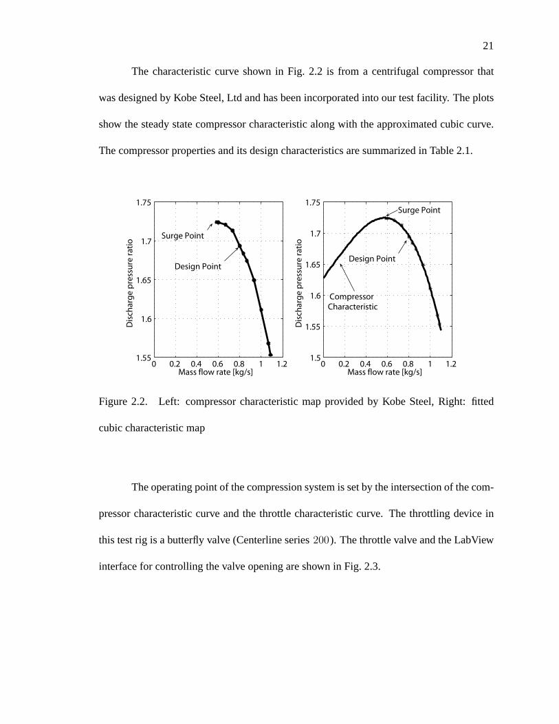
The characteristic curve shown in Fig. 2.2 is from a centrifugal compressor that

was designed by Kobe Steel, Ltd and has been incorporated into our test facility. The plots

show the steady state compressor characteristic along with the approximated cubic curve.

The compressor properties and its design characteristics are summarized in Table 2.1.

0 0.2 0.4 0.6 0.8 1 1.21.55

1.6

1.65

1.7

1.75

Mass flow rate [kg/s]

Dis

char

ge p

ress

ure

ratio

0 0.2 0.4 0.6 0.8 1 1.21.5

1.55

1.6

1.65

1.7

1.75


Dis

char

ge p

ress

ure

ratio

Surge Point

Design PointDesign Point

Surge Point

Compressor Characteristic

Figure 2.2. Left: compressor characteristic map provided by Kobe Steel, Right: fitted

cubic characteristic map

The operating point of the compression system is set by the intersection of the com-

pressor characteristic curve and the throttle characteristic curve. The throttling device in

this test rig is a butterfly valve (Centerline series 200). The throttle valve and the LabView

interface for controlling the valve opening are shown in Fig. 2.3.

22

Table 2.1. Compressor properties

Design speed 23,000 [RPM]

Design mass flow rate 0.833 [kg/sec]

Design pressure ratio 1.68[-]

Inducer hub diameter 56.3[mm]

Inducer tip diameter 116.72[mm]

Impeller exit diameter 250[mm]

Blade height at impeller exit 8.21[mm]

Figure 2.3. Left: Throttle valve, Right: LabView interface for controlling the throttle

valve opening

23

2.1.1 Nondimensionalization

Nondimensional variables are used to model the compression system. Pressure and

mass flow rate are commonly nondimensionalized by 12ρU2 and ρUAc , respectively. This

way the nondimensioanl pressure is a measure of the actual work put in the flow (∆P )

compared to the available work (U2 ), and the nondimensional mass flow rate is just the

axial velocity parameter:

Φc =ρCxAc

ρUAc

=Cx

U(2.2)

where ρ is the inlet air density, U is the impeller tip speed, Ac is the area of the impeller

eye and Cx is the axial velocity. Time is nondimensionalized by the Helmholtz frequency,

ωH :

ωH = ao1

√Ac

VpLc

(2.3)

where Vp is the plenum volume, Lc is the length of the compressor duct and ao1 is the

ambient speed of sound. The dimensionless mass flow rate through the throttle valve is

commonly modeled as [50]:

Φth = cthuth

√Ψp (2.4)

where cth is the valve constant, uth is the percent throttle opening, Φth is the nondimen-

sional throttle mass flow rate and Ψp is the nondimensional plenum pressure rise:

Φth =mth

ρUAc

and Ψp =∆Pp

12ρU2

(2.5)

The compressor characteristic curve, (2.1), is nondimensionalized using the same nondi-

mensional coefficients:

ψc,ss = Am3c +Bm2

c + Cmc +D

24

= A(ρUA)3︸︷︷︸A1

Φ3c +B(ρUA)2︸︷︷︸

B1

Φ2c + C(ρUA)︸︷︷︸

C1

Φc +D

= A1Φ3c +B1Φ

2c + C1Φc +D (2.6)

Ψc,ss =∆Pc,ss

12ρU2

=Pc,ss − Po1

12ρU2

=Po1 (ψc,ss − 1)

12ρU2

(2.7)

The equilibrium values (operating points) are found from the intersection of the throttle

and the compressor characteristics. From the compressor characteristic curve:

Ψeq =Po1

12ρU2

(ψc,ss(Φceq) − 1) (2.8)

=Po1

12ρU2

(A1Φ

3ceq

+B1Φ2ceq

+ C1Φceq +D − 1)

(2.9)

from the throttle characteristic, (2.4):

Ψp =Φ2

th

c2thu2th

(2.10)

At the equilibrium point Ψeq = Ψp and Φceq = Φth , therefore Φeq is found from solving

the following equation:

A1Φ3ceq

+

(B1 −

12ρU2

Po1c2thu2th

)Φ2

ceq+ C1Φceq +D − 1 = 0 (2.11)

The nondimensional compressor characteristic along with various throttle settings are shown

in Fig. 2.4.

2.2 Greitzer Compression System Model

In 1976, Greitzer [22] developed a model for a compression system consisting of a

compressor, a plenum volume and a throttle valve. Such a compression system is shown in

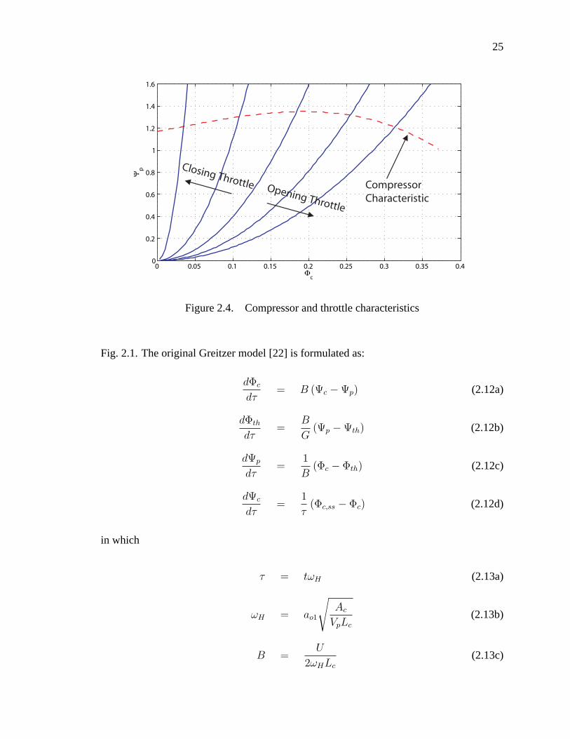
25

0 0.05 0.1 0.15 0.2 0.25 0.3 0.35 0.40

0.2

0.4

0.6

0.8

1

1.2

1.4

1.6

Ψp

Φc

Closing Throttle Opening Throttle


Figure 2.4. Compressor and throttle characteristics

Fig. 2.1. The original Greitzer model [22] is formulated as:

dΦc

dτ= B (Ψc − Ψp) (2.12a)

dΦth

dτ=

B

G(Ψp − Ψth) (2.12b)

dΨp

dτ=

1

B(Φc − Φth) (2.12c)

dΨc

dτ=

1

τ(Φc,ss − Φc) (2.12d)

in which

τ = tωH (2.13a)

ωH = ao1

√Ac

VpLc

(2.13b)

B =U

2ωHLc

(2.13c)

26

G =LthAc

LcAth

(2.13d)

where the subscript c refers to the compressor, p to the plenum, th to the throttle and 1

to the ambient values. Φ is the nondimensional mass flow rate, Ψ is the nondimensional

pressure rise, and ωH is the Helmholtz frequency as defined earlier.

Equation 2.12a is the 1-D momentum equation for the compressor duct. Equation

2.12b is the 1-D momentum equation for the throttle duct. Equation 2.12c is the mass

balance for the plenum volume. Equation 2.12d describes the dynamics of the compressor

characteristic curve.

This model has been developed assuming: one dimensional incompressible flow

in the ducts, isentropic compression process, uniform pressure distribution and negligible

velocity in the plenum, insignificant rotor speed variations, quasi-steady compressor and

throttle behavior and negligible temperature rise in the overall system. The compressor and

throttling device are both modeled as actuator disks, i.e. planes with continuous mass flow

and discontinuous pressure across. Since the oscillations associated with compressor surge

have low frequencies, the wavelength of the pressure oscillations is large compared to the

length of the compressor duct, and the flow in the ducts can be assumed incompressible.

Thus, the compressibility effects are associated with the compression in the plenum volume

while inertia effects are lumped on the acceleration of the gas in the compressor duct [50].

The complete derivation of the model is provided in [22]. Equation (2.12d) was

presented to account for the time lag between the onset of instability and the establishment

of the fully developed rotating stall. Rotating stall plays an important roll in the dynamics

of axial compressors. Therefore, Greitzer introduced a simple first order transient response

27

model to simulate this lag in the response of axial compressors. However, rotating stall

does not influence the performance of centrifugal compressors to nearly the same extent

as previously discussed in Section 1.1.1. Therefore, the compressor is assumed to behave

quasi-stationary to changes in mass flow rate and (2.12d) can be ignored [50].

The G parameter is a measure of the inertia effects in the throttle duct compared

to the inertia effects in the compressor duct. Since the length of the throttle duct Lth is

significantly shorter than the length of the compressor duct Lc , the G parameter can be

assumed to be small and therefore (2.12b) can be ignored. The final nondimensioanl model

of the compression system becomes:

Ψp =ωH

B(Φc − Φth) (2.14a)

Φc = BωH (Ψc − Ψp) (2.14b)

This model was originally developed for a low pressure ratio axial compressor.

However, as discussed earlier, the model has been successfully applied to model various

centrifugal compressors.

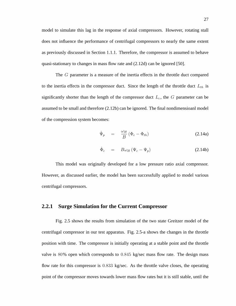
2.2.1 Surge Simulation for the Current Compressor

Fig. 2.5 shows the results from simulation of the two state Greitzer model of the

centrifugal compressor in our test apparatus. Fig. 2.5-a shows the changes in the throttle

position with time. The compressor is initially operating at a stable point and the throttle

valve is 80% open which corresponds to 0.845 kg/sec mass flow rate. The design mass

flow rate for this compressor is 0.833 kg/sec. As the throttle valve closes, the operating

point of the compressor moves towards lower mass flow rates but it is still stable, until the

28

operating point reaches the surge point. At this time, both pressure ratio and mass flow rate

start to oscillate. Further closing the throttle valve causes the compressor to enter the surge

cycle. The surge cycle has a frequency of approximately 6 Hz. The nondimensionalized

pressure ratio and mass flow rate oscillations are plotted in Fig. 2.5-c and .2.5-d. The surge

cycle along with the steady state compressor characteristic curve are shown in Fig. 2.5-b.

Surge occurs at approximately 52% throttle opening which corresponds to 0.567 kg/sec

mass flow rate.

Figure 2.5. Simulation of the compression system using Greitzer’s model

29

2.3 Tip Clearance Effects

There are two types of centrifugal impellers: shrouded or closed-face impellers and

unshrouded or open-face impellers as shown in Fig. 2.6. In shrouded impellers there is a

shroud attached to the blades that rotates with the impeller. There is a clearance between

the rotating shroud and the stationary casing. In unshrouded impellers the space between

the impeller blades and the adjacent stationary shroud is clear. There is an optimum value

for the blade tip clearance [42], therefore, unshrouded impellers have superior performance

over shrouded impellers of identical design.

Unshrouded (Open) ImpellerShrouded (Closed) Impeller

Figure 2.6. Types of centrifugal impellers

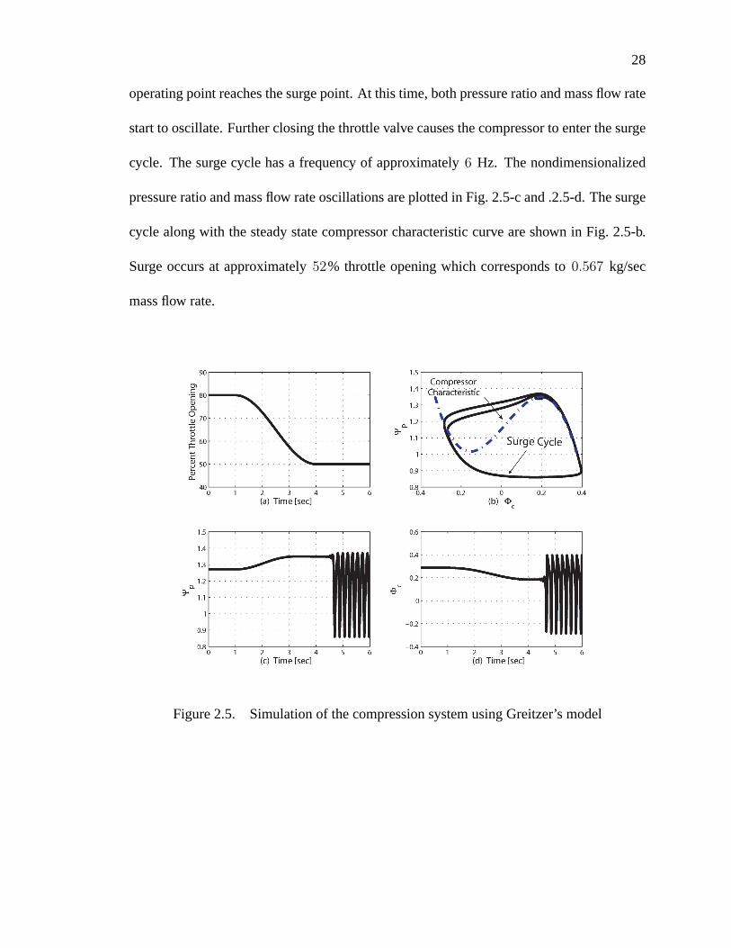
Compressor performance and efficiency are highly dependent on the clearance be-

tween the blade tips and the adjacent shroud. The fluid flow from the pressure side to the

suction side of the compressor blade is referred to as tip leakage. The schematic of the im-

peller blades, the stationary shroud and the tip leakage for both shrouded and unshrouded

impellers is shown in Fig .2.7. The tip clearance effects become very important in high

30

pressure ratio compressors. In such machines, the specific volume of the gas reduces sig-

nificantly at the blade exit, resulting in relatively short design for exit blades. Thus, the

ratio of the tip clearance to the blade height at the impeller exit is relatively high, which

further makes the tip clearance effects significant.

Figure 2.7. Leakage affecting clearance loss in impellers, Top: unshrouded impeller, Bot-

tom: shrouded impeller [5]

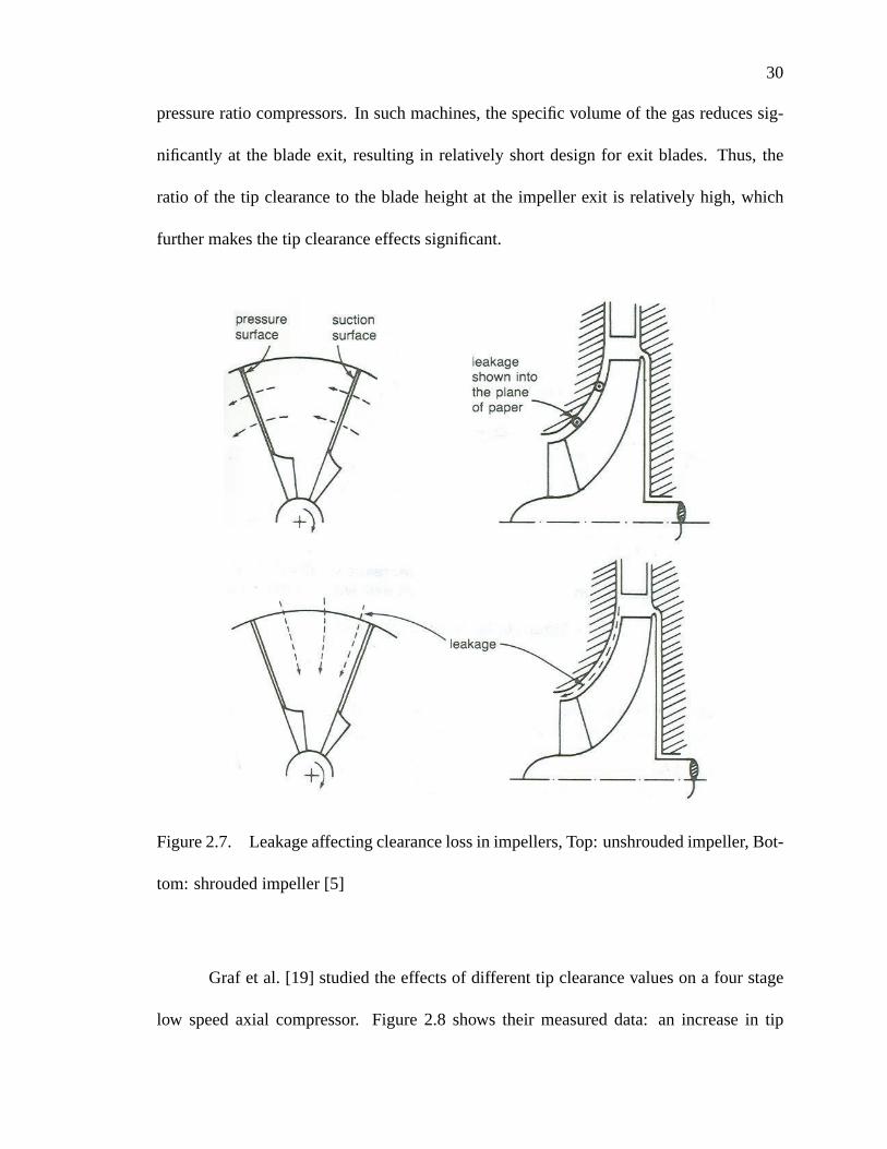
Graf et al. [19] studied the effects of different tip clearance values on a four stage

low speed axial compressor. Figure 2.8 shows their measured data: an increase in tip

31

clearance caused a decrease in peak pressure rise and efficiency as well as an increase

in stalling mass flow and vice versa. The physics of losses due to tip clearance can be

explained as follows: as the tip clearance increases, the induced leakage reduces the energy

transfer from impeller to fluid and decreases the exit velocity angle, which consequently

produces a substantial loss in pressure rise and efficiency.

Figure 2.8. Measured compressor performance with different axisymmetric clearance [19]

The effect of changes in tip clearance is usually expressed as changes in efficiency.

Pampreen [38] measured the average efficiency change for six small gas turbine centrifu-

gal compressors at different clearance values and found that the efficiency change can be

modeled as:

−∆η

η≈ 0.3cl

b2(2.15)

where cl is tip clearance, b2 is the blade height at the impeller exit and η is efficiency

which is compared to the efficiency at zero clearance. Since it is not possible to run the

32

compressor at zero clearance, there are uncertainties in the location of the reference effi-

ciency point. However, the model is not influenced by only the reference point. Eckert et

al. and Pfleiderer [11] individually proposed the following model for the clearance losses:

−∆η

η≈ 2acl

b1 + b2(2.16)

where b1 is the inducer blade height. Eckert et al. suggested a = 0.9 while Pfleiderer

recommended a = 1.5 − 3.0 .

Senoo and Ishida [43] developed a simple model for the leakage loss in centrifugal

compressors. Remarkably good predictions of the loss in efficiency were produced for a

number of compressors. The decrement in efficiency was found to be almost proportional

to the ratio of clearance to blade height at the impeller outlet provided that this ratio is less

than 0.11. The trend is expressed as:

−∆η

η≈ cl

4b2(2.17)

This means that for every 4% change in the ratio of tip clearance variation over the

blade height at the exit, the efficiency changes by 1%. This efficiency loss is smaller at

lower mass flow rates.

The variations in efficiency due to changes in tip clearance are not very large. There-

fore, very high accuracy measurement is required to assess the effects of tip clearance vari-

ations on compressor efficiency. According to Senoo [42], such difficulty in measurement

might be one of the reasons for the variation of empirical equations in the literature.

1As will be discussed in Section 2.4 this is condition is satisfied for the current test rig.

33

Flow patterns at the blade tip region are very complex due to leakage of the flow

through the clearance gap, secondary flows and variations of the blade incidence angle

due to the circumferential motion of the blades relative to the boundary layer flow [42].

The only way to quantitatively assess the tip clearance effects is through computational

models. However, a flow model consisting of only few major parameters that influence

the performance and efficiency due to tip clearance changes and can accurately predict the

losses at different tip clearance values is reasonable and can be used for both understanding

the physics of the tip clearance effects and for control purposes. It is just as easy to obtain

such a dynamic model from CFD as from experiments such as the one done by [42].

2.4 Compressor Model with Tip Clearance Effects

The goal is to provide a model that describes the overall performance of the com-

pressor due to tip clearance variations rather than the detailed dynamic behavior of the

fluid. Senoo’s relation for the effects of static clearance changes on efficiency is used to

develop a model for the compression system that includes tip clearance influence. From

(2.17):

η =η0

1 + 0.25clb2

(2.18)

Therefore, the efficiency at the design clearance is expressed as:

ηd =η0

1 + 0.25cldb2

(2.19)

where the subscript d stands for the design values. This way the efficiency at each tip

clearance value can be described as a function of the efficiency at the design clearance

instead of the zero clearance efficiency:

34

η =ηd

(1 + 0.25cld

b2

)1 + 0.25cl

b2

(2.20)

Define:

δcl = cld − cl (2.21)

i.e. positive δcl indicates moving the impeller towards the stationary shroud. Equation

(2.20) can be written as a function of the design clearance and the clearance variation from

the design clearance:

η =ηd

(1 + 0.25cld

b2

)(1 + 0.25cld

b2

)− 0.25δcl

b2

(2.22)

Define:

k0 =0.25

1 + 0.25cldb2

(2.23)

so that the efficiency at each clearance can be expressed as a function of the design clear-

ance according to:

η =ηd

1 − k0δcl

b2

(2.24)

Based on perfect gas and isentropic compression assumptions, the compressor total to static

isentropic efficiency is:

η =

To1Cp

(ψ

γ−1γ

c − 1

)∆hoc,ideal

(2.25)

where To1 is the inlet stagnation temperature, Cp is the specific heat at constant pressure,

and ∆hoc,ideal is the total specific enthalpy delivered to the fluid.

Using the above relation for efficiency and assuming a quasi-static approximation for the

effects of tip clearance, (2.24) can be rewritten as2:

2the quasi-static assumption is further explained in Section 2.6

35

To1Cp

(ψ

γ−1γ

c − 1

)∆hoc,ideal

=

To1Cp

(ψ

γ−1γ

c,ss − 1

)∆hoc,ideal

(1 − k0

δcl

b2

) (2.26)

Therefore, the compressor pressure ratio as a function of tip clearance variation from the

design clearance can be expressed as:

ψc =

1 +

ψγ−1

γc,ss − 1

1 − k0δcl

b2

γγ−1

(2.27)

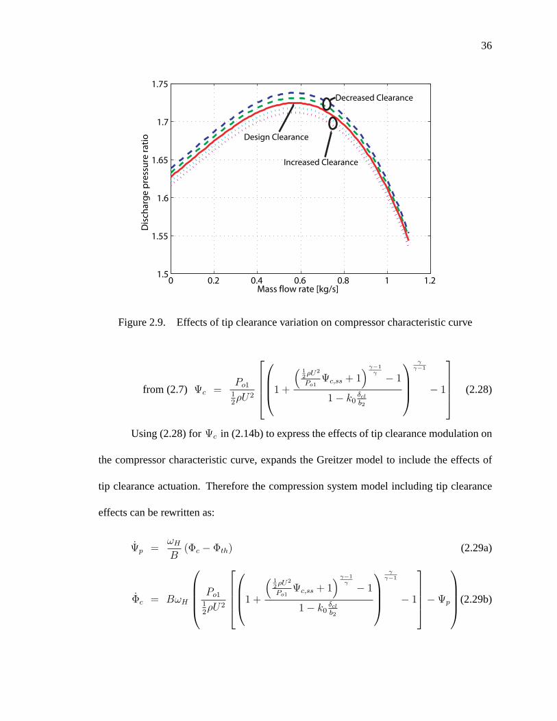
Figure 2.9 shows the simulation of the model derived in (2.27). The solid line rep-

resents the compressor characteristic map at the design clearance. As the tip clearance de-

creases by moving the impeller closer to the stationary shroud, the pressure ratio increases.

Increasing the blade tip clearance by moving the impeller away from the stationary shroud,

decreases the pressure ratio. The model developed by Senoo, (2.17), is valid for clb2< 0.1 .

The blade height at the impeller exit, b2 , in the current compressor is 8 mm and the design

tip clearance is 0.5 mm. Therefore, Senoo’s model is valid for tip clearance increase up to

60% of the design clearance, i.e. 0.8 mm.

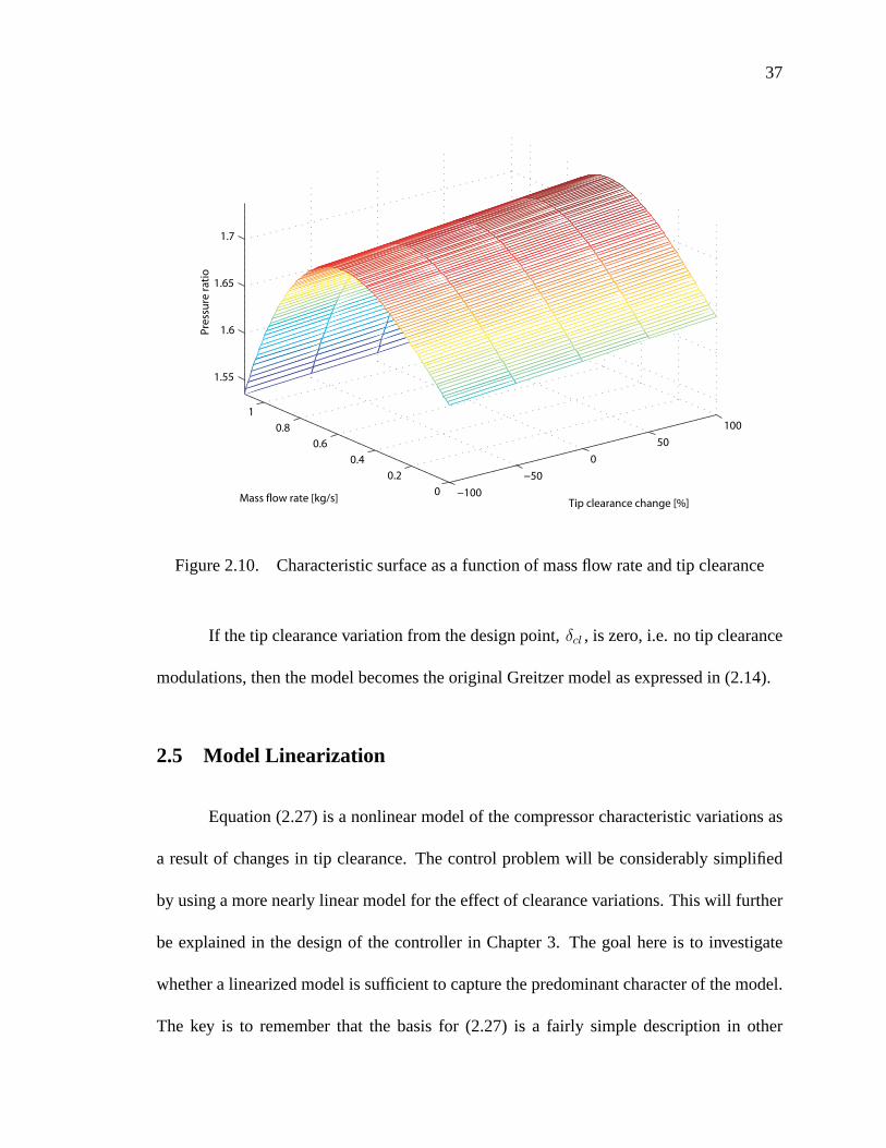
Figure 2.10 shows how the compressor pressure ratio varies with tip clearance

changes at different mass flow rates. To include this model for the effects of tip clearance

actuation in the Greitzer model, the tip clearance model should first be nondimensionalized:

Ψc =∆Pc

12ρU2

=Pc − Po1

12ρU2

=Po1 (ψc − 1)

12ρU2

from (2.27) Ψc =Po1

12ρU2

1 +

ψγ−1

γc,ss − 1

1 − k0δcl

b2

γγ−1

− 1

36

0 0.2 0.4 0.6 0.8 1 1.21.5

1.55

1.6

1.65

1.7

1.75


Dis

char

ge p

ress

ure

ratio Design Clearance

Increased Clearance

Decreased Clearance

Figure 2.9. Effects of tip clearance variation on compressor characteristic curve

from (2.7) Ψc =Po1

12ρU2

1 +

(12ρU2

Po1Ψc,ss + 1

) γ−1γ − 1

1 − k0δcl

b2

γγ−1

− 1

(2.28)

Using (2.28) for Ψc in (2.14b) to express the effects of tip clearance modulation on

the compressor characteristic curve, expands the Greitzer model to include the effects of

tip clearance actuation. Therefore the compression system model including tip clearance

effects can be rewritten as:

Ψp =ωH

B(Φc − Φth) (2.29a)

Φc = BωH

Po1

12ρU2

1 +

(12ρU2

Po1Ψc,ss + 1

) γ−1γ − 1

1 − k0δcl

b2

γγ−1

− 1

− Ψp

(2.29b)

37

−100

−50

0

50

100

00.2

0.40.6

0.81

1.55

1.6

1.65

1.7

Tip clearance change [%]Mass flow rate [kg/s]

Pres

sure

ratio

Figure 2.10. Characteristic surface as a function of mass flow rate and tip clearance

If the tip clearance variation from the design point, δcl , is zero, i.e. no tip clearance

modulations, then the model becomes the original Greitzer model as expressed in (2.14).

2.5 Model Linearization

Equation (2.27) is a nonlinear model of the compressor characteristic variations as

a result of changes in tip clearance. The control problem will be considerably simplified

by using a more nearly linear model for the effect of clearance variations. This will further

be explained in the design of the controller in Chapter 3. The goal here is to investigate

whether a linearized model is sufficient to capture the predominant character of the model.

The key is to remember that the basis for (2.27) is a fairly simple description in other

38

coordinates, (2.24). That “simple” model leads to a complicated model in coordinates

relevant to the control problem. So the question raised here is: Is there a simpler model

that fits the control problem better but is also consistent with the experimental basis for

Senoo’s work? The tip clearance model is therefore linearized as:

ψc ≈

1 +

1 + k0

δclb2

+

(k0δclb2

)2

︸︷︷︸≈0

+ · · ·

(ψ

γ−1γ

c,ss − 1

)γ

γ−1

ψc ≈[ψ

γ−1γ

c,ss − k0δclb2

(1 − ψ

γ−1γ

c,ss

)] γγ−1

ψc ≈ ψc,ss − γ

γ − 1

k0

b2ψ

1γc,ss

(1 − ψ

γ−1γ

c,ss

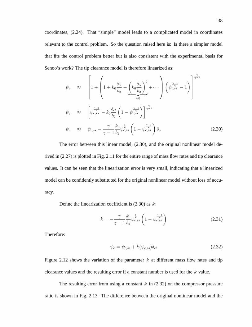
)δcl (2.30)

The error between this linear model, (2.30), and the original nonlinear model de-

rived in (2.27) is plotted in Fig. 2.11 for the entire range of mass flow rates and tip clearance

values. It can be seen that the linearization error is very small, indicating that a linearized

model can be confidently substituted for the original nonlinear model without loss of accu-

racy.

Define the linearization coefficient is (2.30) as k :

k = − γ

γ − 1

k0

b2ψ

1γc,ss

(1 − ψ

γ−1γ

c,ss

)(2.31)

Therefore:

ψc = ψc,ss + k(ψc,ss)δcl (2.32)

Figure 2.12 shows the variation of the parameter k at different mass flow rates and tip

clearance values and the resulting error if a constant number is used for the k value.

The resulting error from using a constant k in (2.32) on the compressor pressure

ratio is shown in Fig. 2.13. The difference between the original nonlinear model and the

39

−100

−50

0

50

100

0

0.5

1

1.5−15

−10

−5

0

5x 10

−3


ψc li

near

izat

ion

erro

r [%

]

Figure 2.11. Tip clearance model linearization error

linearized model assuming a constant k is very small. This shows that at any tip clearance

value, the compressor pressure ratio can be expressed as the steady state compressor char-

acteristic plus the changes in the tip clearance from the design clearance times the constant

coefficient k :

ψc = ψc,ss + kδcl (2.33)

A comparison between the original nonlinear model for the effects of tip clearance

on the compressor pressure ratio, (2.27), and its linear approximation, (2.33), is shown in

Fig. 2.14. The linear model follows the nonlinear model very closely in the regions that

the surge controller is needed. The difference between the two increases at mass flow rates

near zero. However, as was shown in Fig. 2.13 the error is still negligible, e.g. ≈ 0.0015%

at 0.3 kg/sec mass flow rate.

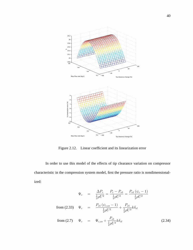
40

−100

−50

0

50

100

0.2

0.4

0.6

0.824.8

25

25.2

25.4

25.6

25.8

26

26.2


k

−100

−50

0

50

100

0.2

0.4

0.6

0.8−3

−2

−1

0

1

2

3


k Li

near

izat

ion

erro

r [%

]

Figure 2.12. Linear coefficient and its linearization error

In order to use this model of the effects of tip clearance variation on compressor

characteristic in the compression system model, first the pressure ratio is nondimensional-

ized:

Ψc =∆Pc

12ρU2

=Pc − Po1

12ρU2

=Po1 (ψc − 1)

12ρU2

from (2.33) Ψc =Po1 (ψc,ss − 1)

12ρU2

+Po1

12ρU2

kδcl

from (2.7) Ψc = Ψc,ss +Po1

12ρU2

kδcl (2.34)

41

−100

−50

0

50

100

0.2

0.4

0.6

0.8−20

−15

−10

−5

0

5

x 10−3


ψc li

near

izat

ion

erro

r [%

]

Figure 2.13. Tip clearance model linearization error using Taylor series

Therefore, the original Greitzer model, (2.14), can be rewritten to include the effects of tip

clearance modulations as:

Ψp =ωH

B(Φc − Φth) (2.35a)

Φc = BωH

(Ψc,ss +

Po1

12ρU2

kδcl − Ψp

)(2.35b)

This set of equations models the compression system and includes the effects of tip

clearance modulations. If the tip clearance variation from the design point is zero, i.e. no tip

clearance modulations, then the model becomes the original Greitzer model as expressed

in (2.14).

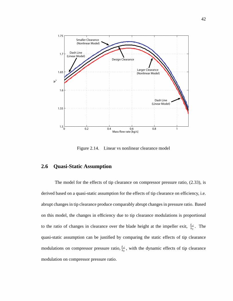
42

0 0.2 0.4 0.6 0.8 11.5

1.55

1.6

1.65

1.7

1.75


ψc

Design Clearance

Larger Clearance(Nonlinear Model)

Smaller Clearance(Nonlinear Model)

Dash Line(Linear Model)

Dash Line(Linear Model)

Figure 2.14. Linear vs nonlinear clearance model

2.6 Quasi-Static Assumption

The model for the effects of tip clearance on compressor pressure ratio, (2.33), is

derived based on a quasi-static assumption for the effects of tip clearance on efficiency, i.e.

abrupt changes in tip clearance produce comparably abrupt changes in pressure ratio. Based

on this model, the changes in efficiency due to tip clearance modulations is proportional

to the ratio of changes in clearance over the blade height at the impeller exit, δcl

b2. The

quasi-static assumption can be justified by comparing the static effects of tip clearance

modulations on compressor pressure ratio, δcl

b2, with the dynamic effects of tip clearance

modulation on compressor pressure ratio.

43

The dynamic effects can be examined by looking at the induced axial velocity be-

cause of axial tip clearance modulation and comparing it to the axial velocity of the fluid,

i.e. nondimensional ratiodcldt

u(the speed induced by tip clearance modulation over the axial

velocity of the fluid). The axial velocity of the fluid at surge point for this compressor is:

u =m

ρAc

=0.56[kg/sec]

1.2[kg/m3]0.0082104[m2]≈ 56[m/sec] (2.36)

Assuming that the modulation is performed at 20 Hz and that the tip clearance vari-

ation is 0.25 mm (i.e. 50% of the available clearance), the ratio of dcldt

is 0.005 , resulting

in adcldt

uof 8.93e − 5 . For the same tip clearance modulation, (i.e. 0.25 mm), the ratio of

δcl

b2for this compressor is 0.03125 . Therefore:

δclb2

dcldt

u

3.12e− 2 8.93e− 5

This means that the dynamic effects of tip clearance,dcldt

u, are indeed negligible

comparing to its static effects, δcl

b2, and a quasi-static assumption can confidently be used to

model the effects of tip clearance modulations on compressor pressure ratio.

2.7 Model Uncertainties

Effects of uncertainties in the linearization coefficient, k in (2.33), on the pressure

ratio is shown in Fig. 2.15. The error between the nonlinear model and the linear model

is plotted for different tip clearance variations from the design value as the linearization

coefficient, k , differs from the value used in the model represented in (2.33). The simu-

lation results are shown at two different mass flow rates. The solid line surface represents

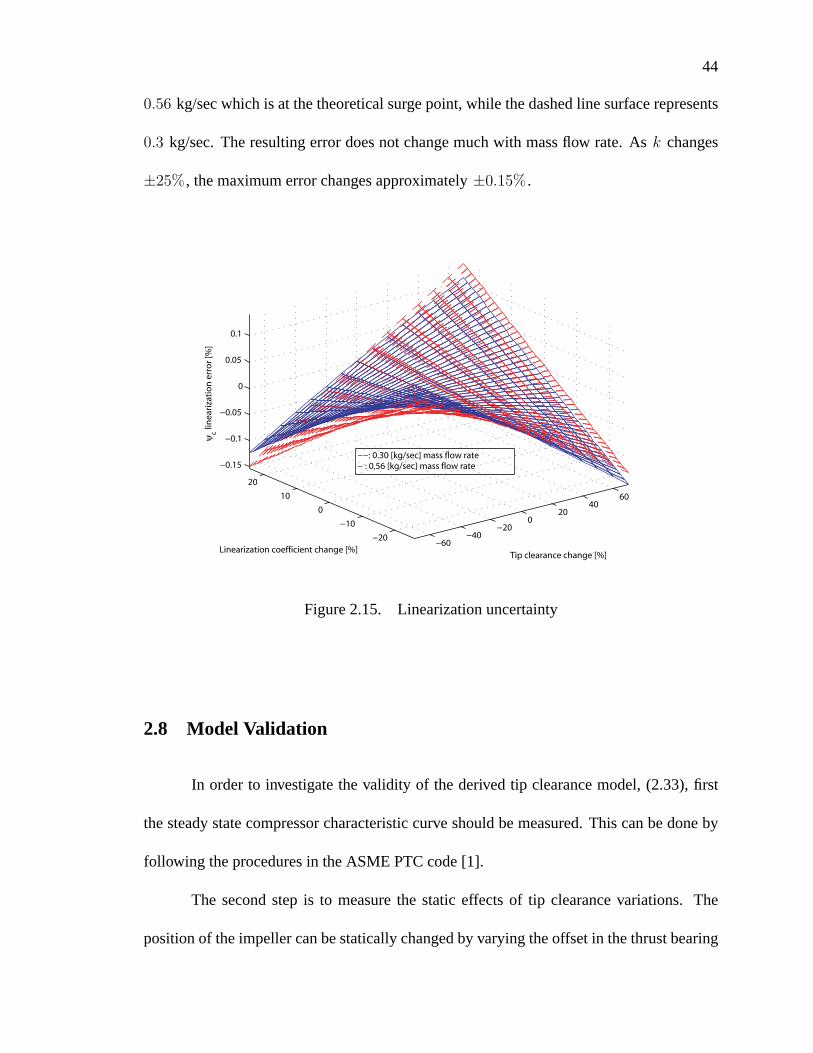
44

0.56 kg/sec which is at the theoretical surge point, while the dashed line surface represents

0.3 kg/sec. The resulting error does not change much with mass flow rate. As k changes

±25% , the maximum error changes approximately ±0.15% .

−60−40

−200

2040

60

−20

−10

0

10

20

−0.15

−0.1

−0.05

0

0.05

0.1

Tip clearance change [%]Linearization coefficient change [%]

ψc li

near

izat

ion

erro

r [%

]

−−: 0.30 [kg/sec] mass flow rate− : 0.56 [kg/sec] mass flow rate

Figure 2.15. Linearization uncertainty

2.8 Model Validation

In order to investigate the validity of the derived tip clearance model, (2.33), first

the steady state compressor characteristic curve should be measured. This can be done by

following the procedures in the ASME PTC code [1].

The second step is to measure the static effects of tip clearance variations. The

position of the impeller can be statically changed by varying the offset in the thrust bearing

45

control algorithm. The mass flow rate will be measured with an orifice meter downstream

the throttle valve, and pressure is measured throughout the compressor and in the plenum

volume. Based on these measurements, the efficiency should be calculated using (2.25),

the parameter k0 should be identified and compared to (2.24). For each throttle setting,

mass flow rate and plenum pressure should be measured at different tip clearance values as

shown in Fig. 2.16 to generate a set of characteristic curves. The measured values should

be compared to the linear and nonlinear model of tip clearance effects, (2.34) and (2.28)

respectively.

0.18 0.2 0.22 0.24 0.26 0.28 0.3 0.32 0.341.1

1.15

1.2

1.25

1.3

1.35

1.4

Φc [−]

Ψc [−

]

Thro

ttle

line

s


lines

Figure 2.16. Procedure for validation of static effects of tip clearance

The last step is to investigate the quasi-static assumption and dynamic effects of tip

clearance modulations. This can be done as follows:

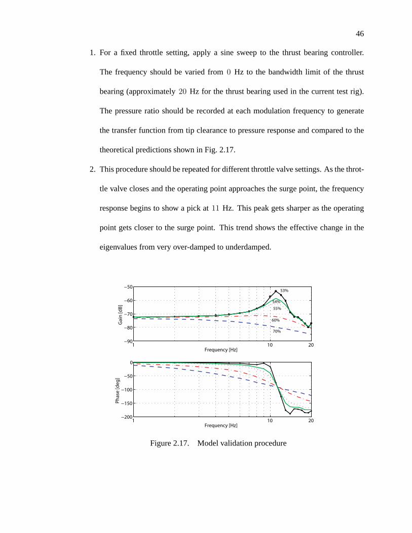
46

1. For a fixed throttle setting, apply a sine sweep to the thrust bearing controller.

The frequency should be varied from 0 Hz to the bandwidth limit of the thrust

bearing (approximately 20 Hz for the thrust bearing used in the current test rig).

The pressure ratio should be recorded at each modulation frequency to generate

the transfer function from tip clearance to pressure response and compared to the

theoretical predictions shown in Fig. 2.17.

2. This procedure should be repeated for different throttle valve settings. As the throt-

tle valve closes and the operating point approaches the surge point, the frequency

response begins to show a pick at 11 Hz. This peak gets sharper as the operating

point gets closer to the surge point. This trend shows the effective change in the

eigenvalues from very over-damped to underdamped.

1 10 20−90

−80

−70

−60

−50

Gai

n [d

B]

Frequency [Hz]

1 10 20−200

−150

−100

−50

0

Phas

e [d

eg]

Frequency [Hz]

60%

70%

55%

54%

53%

Figure 2.17. Model validation procedure

47

3. If the measured values don’t agree with the theoretical prediction, then the quasi-

static assumption might be challenged. If the correlations do agree, then they tend

to lend credence to the quasi-static assumption.

2.9 Summary

Using the known effects of static changes in the tip clearance on compressor para-

meters, a mathematical model was developed to express the sensitivity of the centrifugal

compressor characteristics curve parameters to impeller blade tip clearance. Assuming a

quasi-static approximation for the effects of tip clearance variations induced by axial mo-

tion of the rotor, the existing model for the dynamics of the compression system (Greitzer’s

model [22]) was extended to include the influence of dynamic tip clearance modulation.

The resulting model of the compression system can be used for designing active surge

control systems with tip clearance modulations.

48

CHAPTER 3

ACTIVE CONTROL OF SURGE

The control problem presented by surge is to stabilize a manifold of potential equi-

librium points which lies on the compressor characteristic curve. Without control, all points

on this curve above a specific mass flow rate are stable, while those at lower mass flow rates

are unstable (surge). The problem is complicated by the fact that the specific location on

this manifold is dictated by the throttle setting which, for the problem to be of industrial

interest, must be treated as unknown or at least highly uncertain. This general problem is

further confounded by the specific form of the system: it is nonlinear throughout (not just

at actuation point or sensing point) and cannot readily be transformed to a cascade linear

system with all of the nonlinearity confined to a single state. The ensuing discussion ex-

plores a series of control strategies, each of which moves the solution closer to the goal,

but each of which has shortcomings in accomplishing this goal. The final approach is that

49

of backstepping with uncertainty and an added integral weighting state. This approach is

able to manage all aspects of the problem, although it introduces an algebraically complex

methodology and the solution is consequently hard to interpret. However, simulation re-

sults indicate the effectiveness of the approach and show that substantial changes in throttle

setting, not explicitly known by the controller, may be accommodated to extend the stable

working range of the compressor well beyond its passive range.

3.1 Model

The final model for the compression system, including a nonlinear model for the

effects of tip clearance actuation on the compressor characteristic curve, was presented in

the previous chapter, (2.29):

Ψp =ωH

B(Φc − Φth)

Φc = BωH

Po1

12ρU2

1 +

(12ρU2

Po1Ψc,ss + 1

) γ−1γ − 1

1 − k0δcl

b2

γγ−1

− 1

︸︷︷︸Ψc

−Ψp

The objective of the controller design is stabilize compressor surge, i.e to force the

system trajectories to follow the steady state compressor characteristic curve. Therefore,

the following change of coordinates is applied to move the equilibrium point of the system

to the origin:

Ψp = Ψp − Ψeq (3.1)

50

Φc = Φc − Φeq (3.2)

where the subscript eq stands for the equilibrium values; i.e. the intersection of the steady

state characteristic curves of the compressor characteristic and the throttle valve. Using

this change of coordinates, the model for the compression system becomes:

d

dt(Ψp − Ψeq) =

ωH

B(Φc − Φeq) − ωH

BΦth +

ωH

BΦeq − dΨeq

dt(3.3a)

d

dt(Φc − Φeq) = BωHΨc −BωH (Ψp − Ψeq) −BωHΨeq − dΦeq

dt(3.3b)

where:

dΨeq

dt=

dΨeq

dΦeq

dΦeq

dt(3.4)

dΦeq

dt=

dΦeq

duth

uth (3.5)

Assign:

x = Ψp (3.6)

ξ = Φc (3.7)

Thus, the system of equations (3.3) simplifies to:

x =ωH

Bξ − ωH

BΦth +

ωH

BΦeq − dΨeq

dt(3.8a)

ξ = BωHΨc −BωHΨeq −BωHx− dΦeq

dt(3.8b)

where:

Ψc =Po1

12ρU2

1 +

ψγ−1

γc,ss − 1

1 − k0δcl

b2

γγ−1

− 1

(3.9a)

51

from (2.6) ψc,ss = A1(ξ + Φeq)3 +B1(ξ + Φeq)

2 + C1(ξ + Φeq) +D (3.9b)

from (2.4) Φth = cthuth

√x+ Ψeq (3.9c)

3.2 Stabilization with Mass Flow Feedback

Assume the use of mass flow feedback for tip clearance actuation via the control

law:

δcl = −kpξ (3.10)

where kp is a constant gain. A sufficient condition for the equilibrium point to be globally

exponentially stable is that the gain kp is chosen such that:

kp >

∂Ψc

∂ξ

∂Ψc

∂δcl

(3.11)

Proof: A Lyapunov function is chosen according to:

V =1

2

(B

ωH

x2 +1

BωH

ξ2

)> 0,∀(x, ξ) = (0, 0) (3.12)

The time derivative of this Lyapunov function is:

V =B

ωH

xx+1

BωH

ξξ (3.13a)

from (3.8) V = x

(ξ − Φth + Φeq − B

ωH

dΨeq

dt

)

+ξ

(Ψc (ξ, δcl)−Ψeq−x− 1

BωH

dΦeq

dt

)(3.13b)

assuming constant throttle position: V = −x (Φth−Φeq)︸︷︷︸V1

+ξ (Ψc (ξ, δcl)−Ψeq)︸︷︷︸V2

(3.13c)

The calculation of V1 is shown in Fig. 3.1. Therefore:

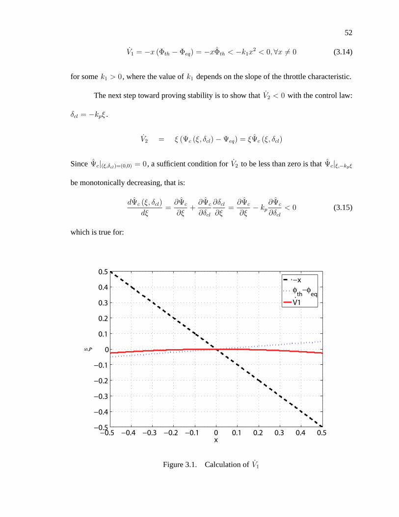
52

V1 = −x (Φth − Φeq) = −xΦth < −k1x2 < 0,∀x = 0 (3.14)

for some k1 > 0 , where the value of k1 depends on the slope of the throttle characteristic.

The next step toward proving stability is to show that V2 < 0 with the control law:

δcl = −kpξ .

V2 = ξ (Ψc (ξ, δcl) − Ψeq) = ξΨc (ξ, δcl)

Since Ψc|(ξ,δcl)=(0,0) = 0 , a sufficient condition for V2 to be less than zero is that Ψc|ξ,−kpξ

be monotonically decreasing, that is:

dΨc (ξ, δcl)

dξ=∂Ψc

∂ξ+∂Ψc

∂δcl

∂δcl∂ξ

=∂Ψc

∂ξ− kp

∂Ψc

∂δcl< 0 (3.15)

which is true for:

−0.5 −0.4 −0.3 −0.2 −0.1 0 0.1 0.2 0.3 0.4 0.5−0.5

−0.4

−0.3

−0.2

−0.1

0

0.1

0.2

0.3

0.4

0.5

x

ξ

−xφ

th−φ

eqV1.

Figure 3.1. Calculation of V1

53

kp >

∂Ψc

∂ξ

∂Ψc

∂δcl

(3.16)

This means that the compression system can be stabilized using tip clearance ac-

tuation (control law: δcl = −kpξ ) if the control gain, kp is chosen such that it is greater

than the ratio of the sensitivity of the compressor characteristic with respect to the mass

flow rate, over the sensitivity of the compressor characteristic with respect to tip clearance

variation.

3.2.1 Simulation Results

Figure 3.2 shows the results of Matlab simulation of the derived model, (3.8), with

mass flow feedback. The required blade tip clearance modulation which is realized using a

magnetic thrust bearing, is calculated according to (3.10).

e

Figure 3.2. Transient response of the compressor with tip clearance actuation (throttling

from 60% to 10%)

54

Changes in the throttle opening reflect disturbances downstream of the compressor.

For the present case, the throttle position was changed from 60% opening (stable region)

to 10% opening (where the compressor would be operating in deep surge if the controller

was not activated) in 3 seconds, Fig. 3.2-(a). The compressor characteristic curve and the

transient response of the system are plotted in Fig. 3.2-(b). Using mass flow feedback for

tip clearance actuation forces the state trajectories to follow the compressor characteristic

curve as the throttle valve continues to move towards the unstable region of the compressor

characteristic curve. The states of the system (nondimensional pressure rise and mass flow

rate) are shown in Fig. 3.2-(c). The mass flow and plenum pressure are well attenuated with

tip clearance actuation, and the compressor reaches the steady operation without instability

despite the extreme changes in the throttle valve. The required tip clearance actuation is

shown in Fig. 3.2-(f). The maximum excursion of the impeller is less than 35% of the

available clearance of the impeller. Using this control scheme, the compression system

is able to withstand extreme changes in the downstream flow conditions with acceptable

control requirement resulting in a significantly extended stable operating region.

To illustrate the effects of the surge controller, the transient response of the com-

pressor without surge controller for the same throttle setting, is shown in Fig. 3.3. As the

mass flow rate reduces with closing the throttle valve (from 60% to 10%), Fig. 3.3-(a), the

compressor enters the deep surge cycles, 3.3-(b), (c) and (d). Using tip clearance modula-

tion with mass flow feedback as in Fig. 3.2, the trajectories would remain on the compressor

characteristic curve, eliminating mass flow and pressure fluctuations associated with com-

pressor surge.

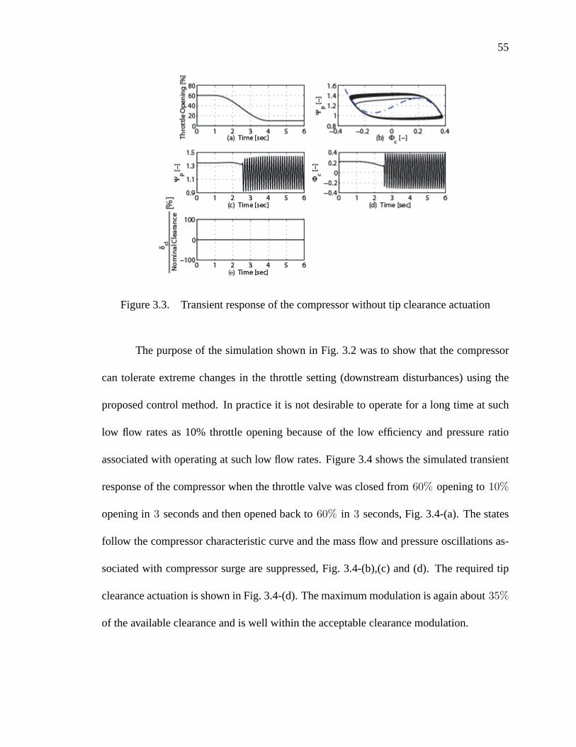
55

e

Figure 3.3. Transient response of the compressor without tip clearance actuation

The purpose of the simulation shown in Fig. 3.2 was to show that the compressor

can tolerate extreme changes in the throttle setting (downstream disturbances) using the

proposed control method. In practice it is not desirable to operate for a long time at such

low flow rates as 10% throttle opening because of the low efficiency and pressure ratio

associated with operating at such low flow rates. Figure 3.4 shows the simulated transient

response of the compressor when the throttle valve was closed from 60% opening to 10%

opening in 3 seconds and then opened back to 60% in 3 seconds, Fig. 3.4-(a). The states

follow the compressor characteristic curve and the mass flow and pressure oscillations as-

sociated with compressor surge are suppressed, Fig. 3.4-(b),(c) and (d). The required tip

clearance actuation is shown in Fig. 3.4-(d). The maximum modulation is again about 35%

of the available clearance and is well within the acceptable clearance modulation.

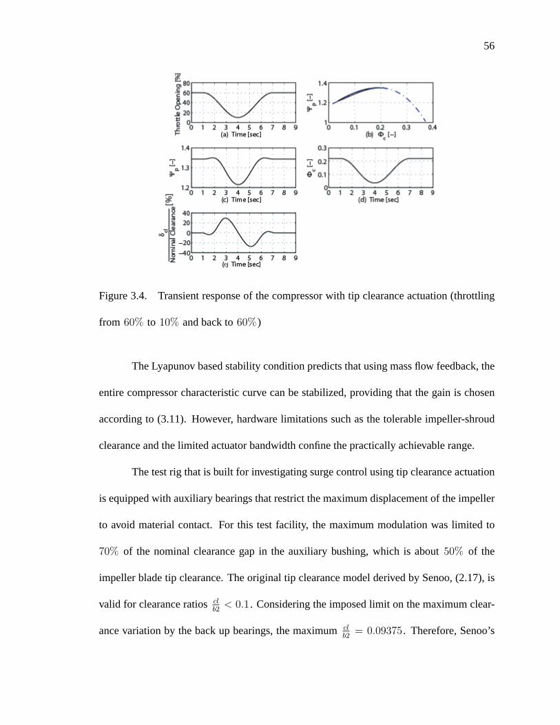
56

e

Figure 3.4. Transient response of the compressor with tip clearance actuation (throttling

from 60% to 10% and back to 60%)

The Lyapunov based stability condition predicts that using mass flow feedback, the

entire compressor characteristic curve can be stabilized, providing that the gain is chosen

according to (3.11). However, hardware limitations such as the tolerable impeller-shroud

clearance and the limited actuator bandwidth confine the practically achievable range.

The test rig that is built for investigating surge control using tip clearance actuation

is equipped with auxiliary bearings that restrict the maximum displacement of the impeller

to avoid material contact. For this test facility, the maximum modulation was limited to

70% of the nominal clearance gap in the auxiliary bushing, which is about 50% of the

impeller blade tip clearance. The original tip clearance model derived by Senoo, (2.17), is

valid for clearance ratios clb2< 0.1 . Considering the imposed limit on the maximum clear-

ance variation by the back up bearings, the maximum clb2

= 0.09375 . Therefore, Senoo’s

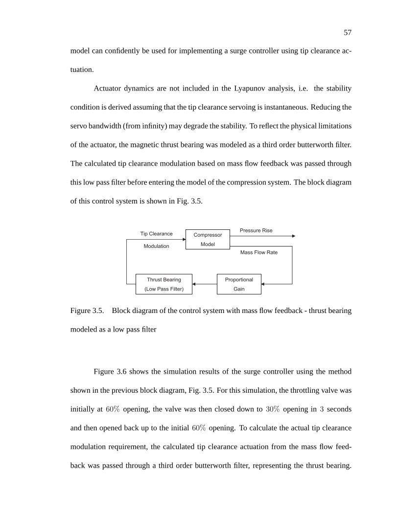
57

model can confidently be used for implementing a surge controller using tip clearance ac-

tuation.

Actuator dynamics are not included in the Lyapunov analysis, i.e. the stability

condition is derived assuming that the tip clearance servoing is instantaneous. Reducing the

servo bandwidth (from infinity) may degrade the stability. To reflect the physical limitations

of the actuator, the magnetic thrust bearing was modeled as a third order butterworth filter.

The calculated tip clearance modulation based on mass flow feedback was passed through

this low pass filter before entering the model of the compression system. The block diagram

of this control system is shown in Fig. 3.5.

Compressor

Model

Proportional

Gain

Thrust Bearing

(Low Pass Filter)

Tip Clearance

Modulation

Pressure Rise

Mass Flow Rate

Figure 3.5. Block diagram of the control system with mass flow feedback - thrust bearing

modeled as a low pass filter

Figure 3.6 shows the simulation results of the surge controller using the method

shown in the previous block diagram, Fig. 3.5. For this simulation, the throttling valve was

initially at 60% opening, the valve was then closed down to 30% opening in 3 seconds

and then opened back up to the initial 60% opening. To calculate the actual tip clearance

modulation requirement, the calculated tip clearance actuation from the mass flow feed-

back was passed through a third order butterworth filter, representing the thrust bearing.

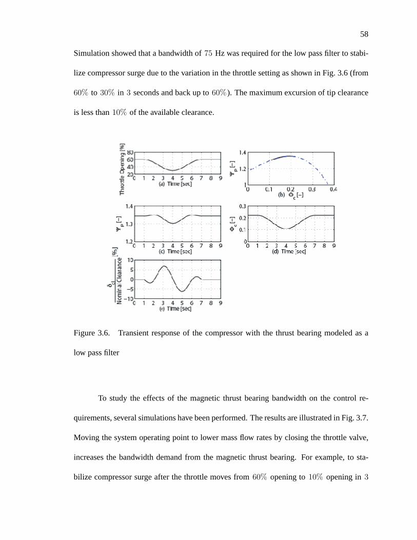
58

Simulation showed that a bandwidth of 75 Hz was required for the low pass filter to stabi-

lize compressor surge due to the variation in the throttle setting as shown in Fig. 3.6 (from

60% to 30% in 3 seconds and back up to 60%). The maximum excursion of tip clearance

is less than 10% of the available clearance.

e

Figure 3.6. Transient response of the compressor with the thrust bearing modeled as a

low pass filter

To study the effects of the magnetic thrust bearing bandwidth on the control re-

quirements, several simulations have been performed. The results are illustrated in Fig. 3.7.

Moving the system operating point to lower mass flow rates by closing the throttle valve,

increases the bandwidth demand from the magnetic thrust bearing. For example, to sta-

bilize compressor surge after the throttle moves from 60% opening to 10% opening in 3

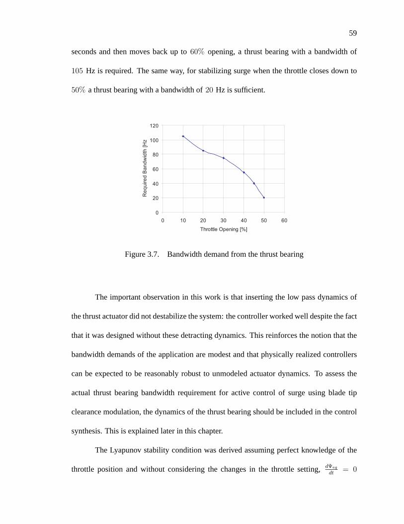
59

seconds and then moves back up to 60% opening, a thrust bearing with a bandwidth of

105 Hz is required. The same way, for stabilizing surge when the throttle closes down to

50% a thrust bearing with a bandwidth of 20 Hz is sufficient.

0

20

40

60

80

100

120

0 10 20 30 40 50 60

Throttle Opening [%]

Req

uire

d B

andw

idth

[Hz

Figure 3.7. Bandwidth demand from the thrust bearing

The important observation in this work is that inserting the low pass dynamics of

the thrust actuator did not destabilize the system: the controller worked well despite the fact

that it was designed without these detracting dynamics. This reinforces the notion that the

bandwidth demands of the application are modest and that physically realized controllers

can be expected to be reasonably robust to unmodeled actuator dynamics. To assess the

actual thrust bearing bandwidth requirement for active control of surge using blade tip

clearance modulation, the dynamics of the thrust bearing should be included in the control

synthesis. This is explained later in this chapter.

The Lyapunov stability condition was derived assuming perfect knowledge of the

throttle position and without considering the changes in the throttle setting, dΨeq

dt= 0

60

and dΦeq

dt= 0 in (3.13b). This reduces the utility of the method when throttle position

is viewed as a model for downstream disturbances. The ultimate goal for control design

is to stabilize compressor surge by properly accommodating for the lack of knowledge of

the throttle setting and its variations. The next section provides a deep insight into the

challenges associated with designing such a controller.

3.3 Sliding Mode Control

The objective of the surge control design is to force the system trajectories to follow

the compressor characteristic curve. Sliding mode control deals with the problem of getting

the states of a system to track a specific time varying trajectory in the presence of model

inaccuracies [45]. Therefore, it might seem that the obvious solution to fulfill the surge

control objective is using the sliding mode method.

Consider the single input dynamic system:

x(n) = f(ξ) + b(ξ)u (3.17)

where the notation x(n) denotes the i th time derivative of x and:

ξ = xx · · · x(n−1)

The tracking error vector ξ is defined as:

ξ = ξ − ξd = x ˙x...x(n−1)

where the subscript d stands for the desired values. The goal is to make the states follow

their desired values. To achieve this, sliding mode control suggests to define a time-varying

sliding function, s(ξ; t) , as:

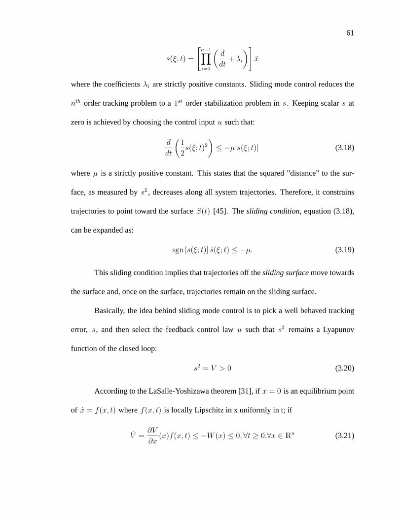
61

s(ξ; t) =

[n−1∏i=1

(d

dt+ λi

)]x

where the coefficients λi are strictly positive constants. Sliding mode control reduces the

nth order tracking problem to a 1st order stabilization problem in s . Keeping scalar s at

zero is achieved by choosing the control input u such that:

d

dt

(1

2s(ξ; t)2

)≤ −µ|s(ξ; t)| (3.18)

where µ is a strictly positive constant. This states that the squared ”distance” to the sur-

face, as measured by s2 , decreases along all system trajectories. Therefore, it constrains

trajectories to point toward the surface S(t) [45]. The sliding condition, equation (3.18),

can be expanded as:

sgn [s(ξ; t)] s(ξ; t) ≤ −µ. (3.19)

This sliding condition implies that trajectories off the sliding surface move towards

the surface and, once on the surface, trajectories remain on the sliding surface.

Basically, the idea behind sliding mode control is to pick a well behaved tracking

error, s , and then select the feedback control law u such that s2 remains a Lyapunov

function of the closed loop:

s2 = V > 0 (3.20)

According to the LaSalle-Yoshizawa theorem [31], if x = 0 is an equilibrium point

of x = f(x, t) where f(x, t) is locally Lipschitz in x uniformly in t; if

V =∂V

∂x(x)f(x, t) ≤ −W (x) ≤ 0,∀t ≥ 0.∀x ∈ Rn (3.21)

62

where V : Rn → R+ is a continuously differentiable, positive definite and radially un-

bounded function and W (x) is positive definite, then the equilibrium x = 0 is globally

uniformly asymptotically stable.

Using (3.20), the condition (3.21) can be rewritten in terms of the sliding function

s as:

2ss ≤ −W (3.22)

Choosing

W = 2ηs > 0 and η > 0 (3.23)

the condition (3.22) becomes:

2ss < −2ηs (3.24)

or

sgn(s)s < −η (3.25)

which is the same as the sliding condition introduced in (3.19). The system dynamics while

in sliding mode can be described as:

s = 0 (3.26)

The control input resulting from solving (3.32) is called the equivalent control, ueq ,

which is the control input that would maintain s = 0 if the system dynamics were exactly

known. Therefore, s can be rewritten as:

s = k0 (u− ueq) (3.27)

i.e if s = 0 → u = ueq

63

choose u = ueq − k1sgn(s) (3.28)

then s = k0 (ueq − k1sgn(s) − ueq) = −k1sgn(s) (3.29)

→ sgn(s)s = −sgn(s)k1sgn(s) < −η ∀k1 > η (3.30)

3.4 Sliding Mode for Surge Control

In order to use sliding mode method for designing a surge controller the linearized

model for the effects of tip clearance as previously derived in (2.35a) is used to model the

compression system:

Ψp =ωH

B(Φc − Φth)

Φc = BωH

(Ψc,ss +

Po1

12ρU2

kδcl − Ψp

)

Since the control objective in surge mitigation is to force the system trajectories

to follow the nominal compressor characteristic, define the sliding surface to be the steady

state compressor characteristic. This characteristic represents an equilibrium in phase space

parameterized by throttle setting: surge arises because this equilibrium is not everywhere

stable.

s = Ψp − Ψc,ss (3.31)

The system dynamic while in sliding mode can be expressed as:

s = 0. (3.32)

The equivalent control, which is the continuous control law that would maintain

s = 0 , can be obtained by solving (3.32) for the control input u .

64

s = Ψp − ∂Ψc,ss

∂Φc

Φc = 0 (3.33)

from (2.35a) ueq =ωH

B(Φc − Φth) − ∂Ψc,ss

∂ΦcBωH (Ψc,ss − Ψp)

BωHPo1

12ρU2k

∂Ψc,ss

∂Φc

(3.34)

The equivalent control resulting from the sliding function introduced in (3.31) re-

quires division by ∂Ψc,ss

∂Φcwhich is zero at the peak of the compressor characteristic curve,

Fig. 2.4. Therefore, the state trajectories will not follow the compressor characteristic curve

using sliding mode method. Since the objective of the control design is to force the sys-

tem trajectories to remain on the compressor characteristic curve, this curve is the desired

sliding surface. To avoid the singularity at the peak of the characteristic curve, change of

coordinates has been considered. However, it did not solve the singularity problem. The

sliding mode problem formulation requires putting the system model into a cascade of in-

tegrators canonical format. This makes the problem so algebraically complicated that it is

simply intractable, especially if the dynamics of the thrust bearing were to be included in

the control synthesis. Furthermore, the design of a stabilizing controller would depend on

having perfect knowledge of the throttle settings. Which are not available to the controller

in real applications.

3.5 Integrator Backstepping

The backstepping method allows for remaining on the compressor characteristic

curve in the presence of downstream disturbances without the algebraic difficulties associ-

ated with sliding mode method. The actuator dynamics can also be accommodated in the

controller design algorithm. This section provides the constructs that are used in the design

65

of the backstepping controller for surge mitigation. Proofs of these constructs and more

discussion of this methodology can be found in [31], [30] and [35].

Assumption 1: Consider a system of the form:

x = f(x) + g(x)u, f(0) = 0 (3.35)

where x ∈ Rn is the state and u ∈ R is the control input. Assume that there is a con-

tinuously differentiable feedback control law u = α1(x) where α1(0) = 0 and a smooth,

positive definite, radially unbounded function V : Rn → R such that

V (x) =∂V

∂x(x) [f(x) + g(x)α1(x)] ≤ −W (x) ≤ 0,∀x ∈ Rn (3.36)

where W : Rn → R is positive definite. Under this assumption, the control u = α1(x) ,

applied to the system (3.35) renders x = 0 the global asymptotic stable equilibrium of

(3.35).

Let the system(3.35) be augmented by an integrator:

x = f(x) + g(x)ξ (3.37a)

ξ = u (3.37b)

and suppose that (3.37a) satisfies Assumption 1 with ξ ∈ R as its control input. If W (x)

is positive definite, then Va(x, ξ) = V (x) + 12[ξ − α1(x)]

2 is a Control Lyapunov Function

(clf) for the full system (3.37); that is, there exists a feedback control u = αa(x, ξ) which

renders x = 0, ξ = 0 the global asymptotic stable equilibrium of (3.37). According to [31]

one such control is:

u = −k1 [ξ − α1(x)] +∂α1

∂x(x) [f(x) + g(x)ξ] − ∂V

∂x(x)g(x), k1 > 0 (3.38)

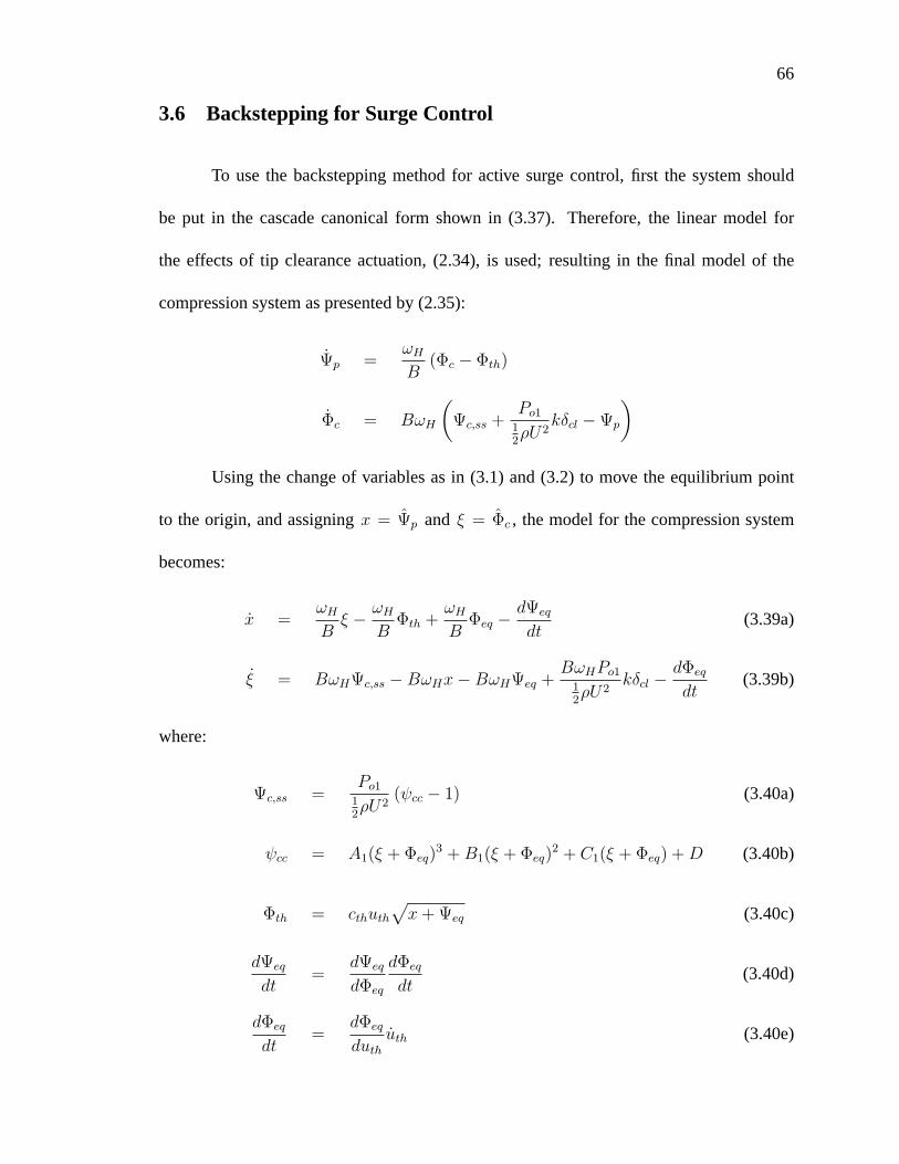
66

3.6 Backstepping for Surge Control

To use the backstepping method for active surge control, first the system should

be put in the cascade canonical form shown in (3.37). Therefore, the linear model for

the effects of tip clearance actuation, (2.34), is used; resulting in the final model of the

compression system as presented by (2.35):

Ψp =ωH

B(Φc − Φth)

Φc = BωH

(Ψc,ss +

Po1

12ρU2

kδcl − Ψp

)

Using the change of variables as in (3.1) and (3.2) to move the equilibrium point

to the origin, and assigning x = Ψp and ξ = Φc , the model for the compression system

becomes:

x =ωH

Bξ − ωH

BΦth +

ωH

BΦeq − dΨeq

dt(3.39a)

ξ = BωHΨc,ss −BωHx−BωHΨeq +BωHPo1

12ρU2

kδcl − dΦeq

dt(3.39b)

where:

Ψc,ss =Po1

12ρU2

(ψcc − 1) (3.40a)

ψcc = A1(ξ + Φeq)3 +B1(ξ + Φeq)

2 + C1(ξ + Φeq) +D (3.40b)

Φth = cthuth

√x+ Ψeq (3.40c)

dΨeq

dt=

dΨeq

dΦeq

dΦeq

dt(3.40d)

dΦeq

dt=

dΦeq

duth

uth (3.40e)

67

Assign:

f(x) = −ωH

BΦth +

ωH

BΦeq − dΨeq

dtf(0) = 0 (3.41a)

g =ωH

B(3.41b)

fa(x, ξ) = −BωHx+BωHΨc,ss(ξ) −BωHΨeq − dΦeq

dt(3.41c)

g1 =BωHPo1

12ρU2

k (3.41d)

so that (3.39) becomes:

x = f(x) + gξ

ξ = fa(x, ξ) + g1δcl

Define:

G1 =δclcl0

(3.42a)

ga = g1cl0 (3.42b)

G0 = fa(x, ξ) + gaG1 (3.42c)

where cl0 is the nominal impeller tip clearance. Therefore the system becomes:

x = f(x) + gξ (3.43a)

ξ = G0 (3.43b)

which is in the same format as (3.37) with G0 as the control input for the augmented

system. Assuming that ξ is the control input for (3.43a), we find a Lyapunov function, V1 ,

68

such that ξ = α1 makes x = 0 the global asymptotic equilibrium of (3.43a). Choose:

V1 =1

2x2 (3.44)

so that the derivative is:

V1 =∂V1

∂xx = x (f(x) + gα1(x))

If

α1(x) =−1

g(f(x) + k0x) (3.45)

then V1 = −k0x2 < 0 . To find the control input G0 for the augmented system (3.43),

define:

V2 = V1 +g

2λ1

[ξ − α1]2 (3.46)

then:

V2 =∂V1

∂xx+

g

λ1

[ξ − α1][ξ − ∂α1

∂xx]

=∂V1

∂x[f + gξ] +

g

λ1

[ξ − α1][G0 − ∂α1

∂xx]

=∂V1

∂x[f + gα1 − gα1 + gξ] +

g

λ1

[ξ − α1][G0 − ∂α1

∂xx]

=∂V1

∂x[f + gα1] +

∂V1

∂x[ξ − vα1] g +

g

λ1

[ξ − α1][G0 − ∂α1

∂xx]

=∂V1

∂x[f + gα1]︸︷︷︸

<0

+g

λ1

[ξ − α1]

[λ1∂V1

∂x+G0 − ∂α1

∂xx

]

Choose:

G0 = α2(x, ξ) = −k1[ξ − α1] +∂α1

∂xx− λ1

∂V1

∂x(3.47)

so that

69

V2 =∂V1

∂x[f + gα1]︸︷︷︸

<0

−k1g

λ1

[ξ − α1]2

→ V2 < 0

Using (3.42c), the tip clearance modulation, u = δcl , that would make x = 0, ξ = 0 the

global asymptotic stable equilibrium, becomes:

G1 = α20 =1

ga

(α2 − fa) (3.48)


Simulation results for the derived backstepping controller are shown in Fig. 3.8.

The simulation is done for the same changes in the throttle setting as in the case of mass

flow feedback, Fig. 3.4. The compressor characteristic curve and the transient response

of the system are again plotted in figure 3.8-b. Using the backstepping controller for tip

clearance actuation, the state trajectories follow the compressor characteristic curve as the

throttle valve continues to move in the unstable region of the compressor and the trajectories

remain on the characteristic curve as the valve opens. The required tip clearance actuation

using the backstepping method along with the required actuation from mass flow feedback

is shown in figure 3.8-e. The maximum modulation of the impeller is less than 15% of

the available clearance using the backstepping method (compared to roughly 30% for mass

flow feedback). It should be noted that, even though a linearized model for the effects of tip

clearance was used to design the controller, (2.35b), the original nonlinear model,(2.29b),

has been used to model the system dynamics in the simulations.

70

[%]

Figure 3.8. Transient response of the compressor with tip clearance actuation using back-

stepping method

3.7 Thrust Bearing Dynamics

To take account of the dynamic limitations of the actuator, the dynamics of the

thrust bearing should be included in the controller design, assuming the following model

for the thrust bearing:

δcl =4φb

µ0mAg

φc (3.49a)

φc =1

N(V − IR) (3.49b)

where φb is the bias flux, µ0 is the permeability of vacuum, m is the weight of the rotor

and the impeller, Ag is the air gap area, φc is the control flux and N is the number of turns

71

in the coil [41]. It is generally reasonable to assume constant φb and that IR is usually very

small in comparison to V . Defining the nondimensionalized V as u ≡ 4φbV/µ0mNAg ,

produces:

δ(3)cl = u (3.50)

Knowing that

I =2gφ

µ0NAg

(3.51)

produces

δ(3)cl =

2Ibgm

V (3.52)

or

V =gm

2Ibu (3.53)

3.8 Backstepping with Chain of Integrators for Active Control of Surge

Based on (3.42a) and (3.50):

G(3)1 =

δ(3)cl

cl0=

u

cl0(3.54)

Define:

u∗ =u

cl0(3.55)

Therefore the model for the compression system augmented with the thrust bearing dynam-

ics becomes:

x = f(x) + g(x)ξ (3.56a)

ξ = fa(x, ξ) + ga(x, ξ)G1 (3.56b)

72

G1 = G2 (3.56c)

G2 = G3 (3.56d)

G3 = u∗ (3.56e)

in which functions f , g , fa and g1 are as defined in (3.9) and u∗ is the control input to

the thrust bearing. In order to calculate u∗ , first assume the first state of the thrust bearing

model:

x = f(x) + g(x)ξ (3.57a)

ξ = fa(x, ξ) + ga(x, ξ)G1 (3.57b)

G1 = G2 (3.57c)

Define:

X1 =

x

ξ

, f1 =

f(x) + g(x)ξ

fa(x, ξ)

, g1 =

0

ga

(3.58)

so that (3.57) can be rewritten in the cascade format required by backstepping method with

G2 as the control input:

X1 = f1 + g1G1 (3.59a)

G1 = G2 (3.59b)

To find the stabilizing controller G2 , define the Lyapunov function:

V3 = V2 +ga

2λ2

[G1 − α20]2 (3.60)

then:

73

V3 =∂V1

∂xx+

g

λ1

[ξ − α1]

[ξ − ∂α1

∂xx

]+ga

λ2

[G1 − α20]

[G1 − ∂α20

∂xx− ∂α20

∂ξξ

]

=∂V1

∂x[f + gξ] +

g

λ1

[ξ − α1]

[fa + gaG1 − ∂α1

∂xx

]

+ga

λ2

[G1 − α20]

[G2 − ∂α20

∂xx− ∂α20

∂ξξ

]

...

=∂V1

∂x[f + gα1]︸︷︷︸

<0

+g

λ1

[ξ − α1]

[α2 − ∂α1

∂xx+

∂V1

∂xλ1

]︸︷︷︸

<0

+ga

λ2

[G1 − α20]

[G2 − ∂α20

∂xx− ∂α20

∂ξξ +

gλ2

λ1

[ξ − α1]

]

Choose:

G2 = α3 = −k2[G1 − α20] +∂α20

∂xx+

∂α20

∂ξξ − gλ2

λ1

[ξ − α1] (3.61)

to produce, finally:

V3 =∂V1

∂x[f + gα1]︸︷︷︸

<0

+g

λ1

[ξ − α1]

[α2 − ∂α1

∂xx+

∂V1

∂xλ1

]︸︷︷︸

<0

−k2ga

λ2

[G1 − α20]2

→ V3 < 0

Now, Add the second state of the thrust bearing to the chain of integrators:

x = f(x) + g(x)ξ (3.62a)

ξ = fa(x, ξ) + ga(x, ξ)G1 (3.62b)

G1 = G2 (3.62c)

G2 = G3 (3.62d)

74

Define:

X2 =

x

ξ

G1

, f2 =

f(x) + g(x)ξ

fa(x, ξ) + gaG1

0

, g2 =

0

0

1

(3.63)

and (3.62) can be rewritten in the cascade format required by backstepping method with

G3 as the control input:

X2 = f2 + g2G2 (3.64a)

G2 = G3 (3.64b)

To find the stabilizing controller G3 , define the Lyapunov function:

V4 = V3 +1

2λ3

[G2 − α3]2 (3.65)

then:

V4 = V3 +1

λ3

[G2 − α3]

[G2 − ∂α3

∂xx− ∂α3

∂ξξ − ∂α3

∂G1

G1

]

=∂V1

∂x[f + gα1] +

g

λ1

[ξ − α1]

[α2 − ∂α1

∂xx+

∂V1

∂xλ1

]

+ga

λ2

[G1 − α20]

[G2 − ∂α20

∂xx− ∂α20

∂ξξ +

gλ2

λ1

[ξ − α1]

]

+1

λ3

[G2 − α3]

[G3 − ∂α3

∂xx− ∂α3

∂ξξ − ∂α3

∂G1

G1

]

...

=∂V1

∂x[f + gα1]︸︷︷︸

<0

+g

λ1

[ξ − α1]

[α2 − ∂α1

∂xx+

∂V1

∂xλ1

]︸︷︷︸

<0

75

+ga

λ2

[G1 − α20]

[α3 − ∂α20

∂xx− ∂α20

∂ξξ +

gλ2

λ1

[ξ − α1]

]︸︷︷︸

<0

+1

λ3

[G2 − α3]

[G3 − ∂α3

∂xx− ∂α3

∂ξξ − ∂α3

∂G1

G1 +gaλ3

λ2

[G1 − α20]

]

Choose:

G3 = α4 = −k3[G2 − α3] +∂α3

∂xx+

∂α3

∂ξξ +

∂α3

∂G1

G1 − gaλ3

λ2

[G1 − α20] (3.66)

so that

V4 =∂V1

∂x[f + gα1]︸︷︷︸

<0

+g

λ1

[ξ − α1]

[α2 − ∂α1

∂xx+

∂V1

∂xλ1

]︸︷︷︸

<0

+ga

λ2

[G1 − α20]

[α3 − ∂α20

∂xx− ∂α20

∂ξξ +

gλ2

λ1

[ξ − α1]

]︸︷︷︸

<0

−k3

λ3

[G2 − α3]2

→ V4 < 0

Using the preceding procedure, the last state of the thrust bearing is added to the

chain of integrators:

x = f(x) + g(x)ξ (3.67a)

ξ = fa(x, ξ) + ga(x, ξ)G1 (3.67b)

G1 = G2 (3.67c)

G2 = G3 (3.67d)

G3 = u∗ (3.67e)

Define:

76

X3 =

x

ξ

G1

G2

, f3 =

f(x) + g(x)ξ

fa(x, ξ) + gaG1

G2

0

, g3 =

0

0

0

1

(3.68)

Therefore (3.67) can be rewritten as:

X3 = f3 + g3G3 (3.69a)

G3 = u∗ (3.69b)

with u∗ as the control input. To find the control input u∗ , define the Lyapunov function:

V5 = V4 +1

2λ4

[G3 − α4]2 (3.70)

then:

V5 = V4 +1

λ4

[G3 − α4]

[u− ∂α4

∂xx− ∂α4

∂ξξ − ∂α4

∂G1

G1 − ∂α4

∂G2

G2

]

=∂V1

∂x[f + gα1] +

g

λ1

[ξ − α1]

[α2 − ∂α1

∂xx+

∂V1

∂xλ1

]

+ga

λ2

[G1 − α20]

[α3 − ∂α20

∂xx− ∂α20

∂ξξ +

gλ2

λ1

[ξ − α1]

]

+1

λ3

[G2 − α3]

[G3 − ∂α3

∂xx− ∂α3

∂ξξ − ∂α3

∂G1

G1 +gaλ3

λ2

[G1 − α20]

]

+1

λ4

[G3 − α4]

[u− ∂α4

∂xx− ∂α4

∂ξξ − ∂α4

∂G1

G1 − ∂α4

∂G2

G2

]

...

=∂V1

∂x[f + gα1]︸︷︷︸

<0

+g

λ1

[ξ − α1]

[α2 − ∂α1

∂xx+

∂V1

∂xλ1

]︸︷︷︸

<0

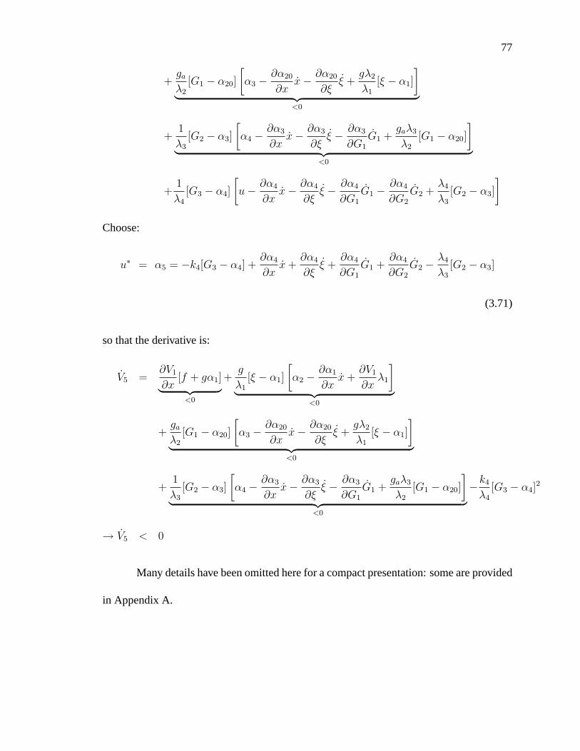
77

+ga

λ2

[G1 − α20]

[α3 − ∂α20

∂xx− ∂α20

∂ξξ +

gλ2

λ1

[ξ − α1]

]︸︷︷︸

<0

+1

λ3

[G2 − α3]

[α4 − ∂α3

∂xx− ∂α3

∂ξξ − ∂α3

∂G1

G1 +gaλ3

λ2

[G1 − α20]

]︸︷︷︸

<0

+1

λ4

[G3 − α4]

[u− ∂α4

∂xx− ∂α4

∂ξξ − ∂α4

∂G1

G1 − ∂α4

∂G2

G2 +λ4

λ3

[G2 − α3]

]

Choose:

u∗ = α5 = −k4[G3 − α4] +∂α4

∂xx+

∂α4

∂ξξ +

∂α4

∂G1

G1 +∂α4

∂G2

G2 − λ4

λ3

[G2 − α3]

(3.71)

so that the derivative is:

V5 =∂V1

∂x[f + gα1]︸︷︷︸

<0

+g

λ1

[ξ − α1]

[α2 − ∂α1

∂xx+

∂V1

∂xλ1

]︸︷︷︸

<0

+ga

λ2

[G1 − α20]

[α3 − ∂α20

∂xx− ∂α20

∂ξξ +

gλ2

λ1

[ξ − α1]

]︸︷︷︸

<0

+1

λ3

[G2 − α3]

[α4 − ∂α3

∂xx− ∂α3

∂ξξ − ∂α3

∂G1

G1 +gaλ3

λ2

[G1 − α20]

]︸︷︷︸

<0

−k4

λ4

[G3 − α4]2

→ V5 < 0

Many details have been omitted here for a compact presentation: some are provided

in Appendix A.

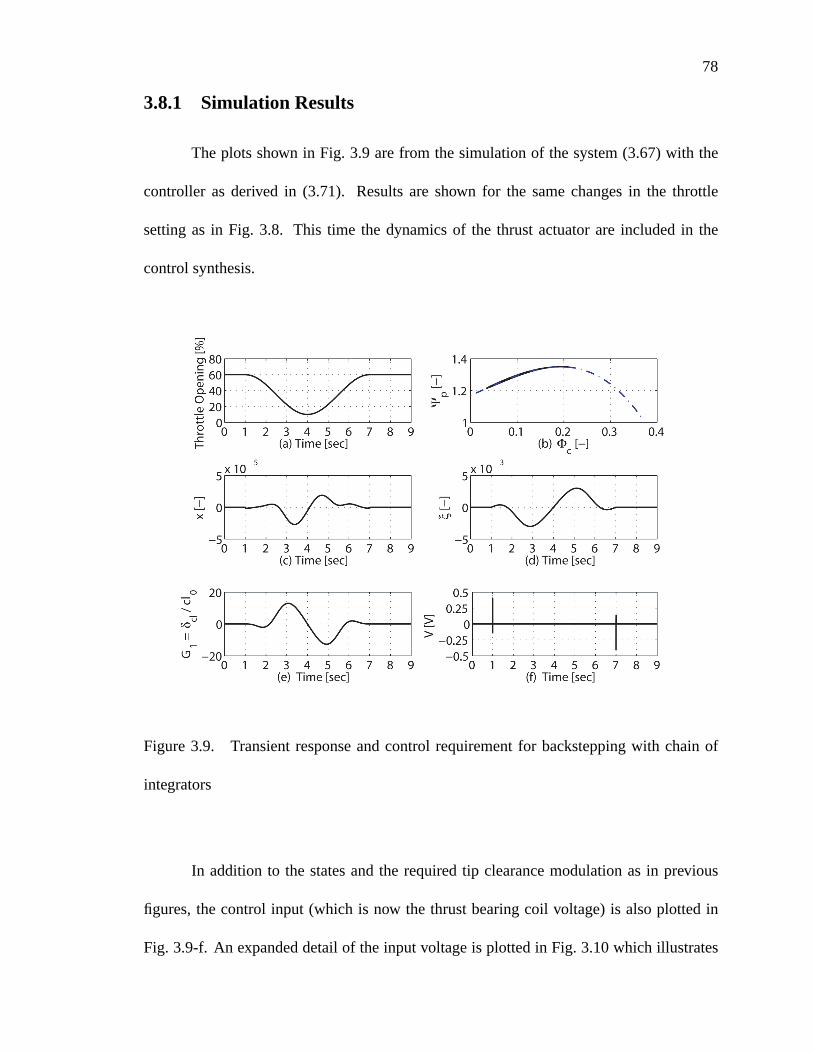
78


The plots shown in Fig. 3.9 are from the simulation of the system (3.67) with the

controller as derived in (3.71). Results are shown for the same changes in the throttle

setting as in Fig. 3.8. This time the dynamics of the thrust actuator are included in the

control synthesis.

Figure 3.9. Transient response and control requirement for backstepping with chain of

integrators

In addition to the states and the required tip clearance modulation as in previous

figures, the control input (which is now the thrust bearing coil voltage) is also plotted in

Fig. 3.9-f. An expanded detail of the input voltage is plotted in Fig. 3.10 which illustrates

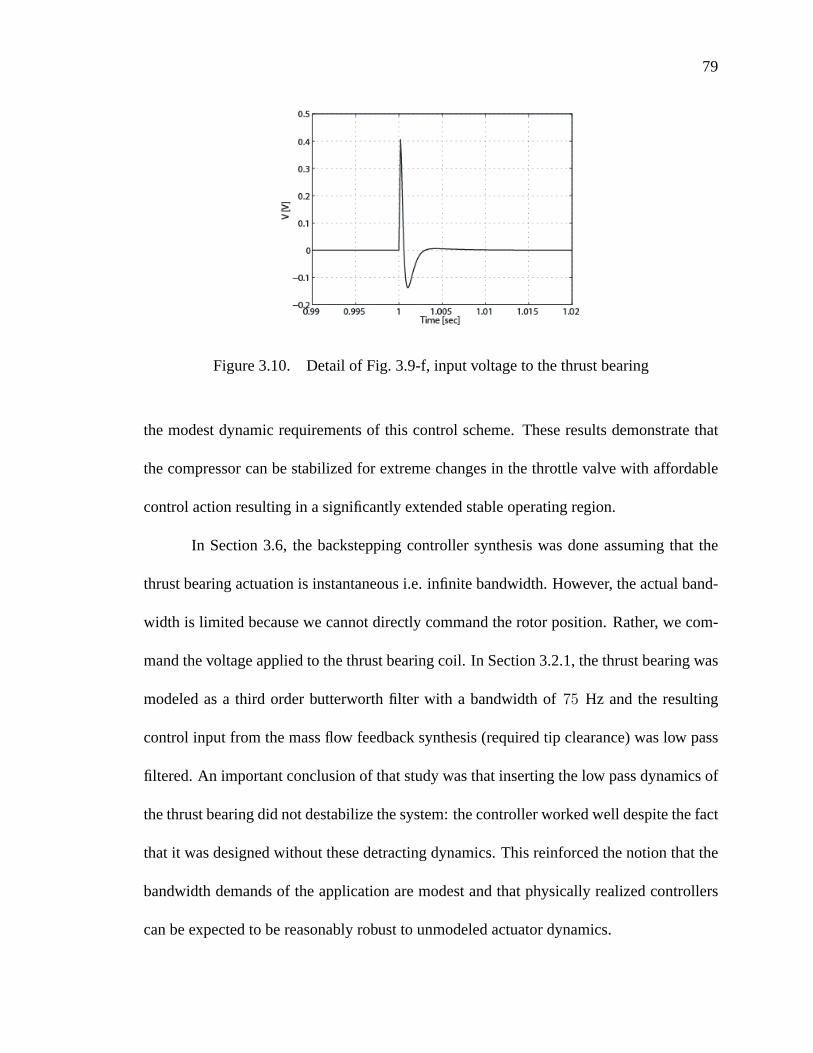
79

Figure 3.10. Detail of Fig. 3.9-f, input voltage to the thrust bearing

the modest dynamic requirements of this control scheme. These results demonstrate that

the compressor can be stabilized for extreme changes in the throttle valve with affordable

control action resulting in a significantly extended stable operating region.

In Section 3.6, the backstepping controller synthesis was done assuming that the

thrust bearing actuation is instantaneous i.e. infinite bandwidth. However, the actual band-

width is limited because we cannot directly command the rotor position. Rather, we com-

mand the voltage applied to the thrust bearing coil. In Section 3.2.1, the thrust bearing was

modeled as a third order butterworth filter with a bandwidth of 75 Hz and the resulting

control input from the mass flow feedback synthesis (required tip clearance) was low pass

filtered. An important conclusion of that study was that inserting the low pass dynamics of

the thrust bearing did not destabilize the system: the controller worked well despite the fact

that it was designed without these detracting dynamics. This reinforced the notion that the

bandwidth demands of the application are modest and that physically realized controllers

can be expected to be reasonably robust to unmodeled actuator dynamics.

80

Including the thrust bearing in the design of the backstepping controller with a chain

of integrators somewhat removes the imposed limit for the required bandwidth of the thrust

bearing. As can be seen in Fig. 3.9, the stable range of the compressor can be signifi-

cantly extended with acceptable control effort. This reinforces the previous observation

that the dynamic requirements of this control strategy are indeed modest which indicates

that control of surge by tip clearance actuation with a thrust bearing can be implemented

in a conventional machine that does not have a specially designed high bandwidth thrust

bearing. Of course no uncertainties were assumed in the throttle position and its derivative

and a triple integrator was used to model the thrust bearing, ignoring the coil resistance and

eddy current effects. Eliminating these simplifications in the control synthesis results in

a much more complicated control structure but does not substantially alter the underlying

result.

Figure 3.11 shows the transient response of the compression system to a sudden

change in the downstream disturbance modeled as a step change in the throttle setting.

The key result is that the maximum required impeller modulation is less than 65% of the

available clearance for a step perturbation from 60% to 50% throttle opening. In reality,

any disturbance in the pipeline will not immediately be transferred to the compressor and

a step change is shown only to indicate the capabilities of the controller.

3.9 Bandwidth Limitations

To assess the bandwidth limitation of the proposed method for surge control, the

linear dependency on G1, G2 and G3 is examined:

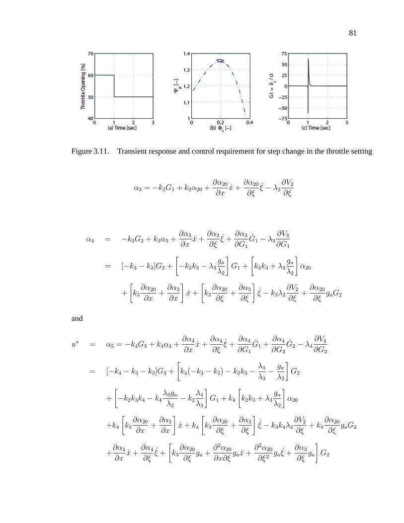
81

Figure 3.11. Transient response and control requirement for step change in the throttle setting

α3 = −k2G1 + k2α20 +∂α20

∂xx+

∂α20

∂ξξ − λ2

∂V2

∂ξ

α4 = −k3G2 + k3α3 +∂α3

∂xx+

∂α3

∂ξξ +

∂α3

∂G1

G1 − λ3∂V3

∂G1

= [−k3 − k2]G2 +

[−k2k3 − λ3

ga

λ2

]G1 +

[k2k3 + λ3

ga

λ2

]α20

+

[k3∂α20

∂x+∂α3

∂x

]x+

[k3∂α20

∂ξ+∂α3

∂ξ

]ξ − k3λ2

∂V2

∂ξ+∂α20

∂ξgaG2

and

u∗ = α5 = −k4G3 + k4α4 +∂α4

∂xx+

∂α4

∂ξξ +

∂α4

∂G1

G1 +∂α4

∂G2

G2 − λ4∂V4

∂G2

= [−k4 − k3 − k2]G3 +

[k4(−k3 − k2) − k2k3 − λ4

λ3

− ga

λ2

]G2

+

[−k2k3k4 − k4

λ3ga

λ2

− k2λ4

λ3

]G1 + k4

[k2k3 + λ3

ga

λ2

]α20

+k4

[k3∂α20

∂x+∂α3

∂x

]x+ k4

[k3∂α20

∂ξ+∂α3

∂ξ

]ξ − k3k4λ2

∂V2

∂ξ+ k4

∂α20

∂ξgaG2

+∂α4

∂xx+

∂α4

∂ξξ +

[k3∂α20

∂ξga +

∂2α20

∂x∂ξgax+

∂2α20

∂ξ2gaξ +

∂α3

∂ξga

]G2

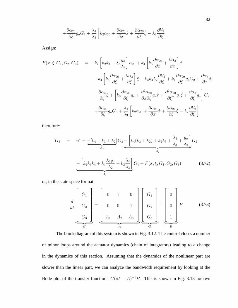
82

+∂α20

∂ξgaG3 +

λ4

λ3

[k2α20 +

∂α20

∂xx+

∂α20

∂ξξ − λ2

∂V2

∂ξ

]

Assign:

F (x, ξ,G1, G2, G3) = k4

[k2k3 + λ3

ga

λ2

]α20 + k4

[k3∂α20

∂x+∂α3

∂x

]x

+k4

[k3∂α20

∂ξ+∂α3

∂ξ

]ξ − k3k4λ2

∂V2

∂ξ+ k4

∂α20

∂ξgaG2 +

∂α4

∂xx

+∂α4

∂ξξ +

[k3∂α20

∂ξga +

∂2α20

∂x∂ξgax+

∂2α20

∂ξ2gaξ +

∂α3

∂ξga

]G2

+∂α20

∂ξgaG3 +

λ4

λ3

[k2α20 +

∂α20

∂xx+

∂α20

∂ξξ − λ2

∂V2

∂ξ

]

therefore:

G3 = u∗ = −[k4 + k3 + k2]︸︷︷︸A3

G3 −[k4(k3 + k2) + k2k3 +

λ4

λ3

+ga

λ2

]︸︷︷︸

A2

G2

−[k2k3k4 + k4

λ3ga

λ2

+ k2λ4

λ3

]︸︷︷︸

A1

G1 + F (x, ξ,G1, G2, G3) (3.72)

or, in the state space format:

d

dt

G1

G2

G3

︸︷︷︸G

=

0 1 0

0 0 1

A1 A2 A3

︸︷︷︸A

G1

G2

G3

︸︷︷︸G

+

0

0

1

︸︷︷︸B

F (3.73)

The block diagram of this system is shown in Fig. 3.12. The control closes a number

of minor loops around the actuator dynamics (chain of integrators) leading to a change

in the dynamics of this section. Assuming that the dynamics of the nonlinear part are

slower than the linear part, we can analyze the bandwidth requirement by looking at the

Bode plot of the transfer function: C(sI − A)−1B . This is shown in Fig. 3.13 for two

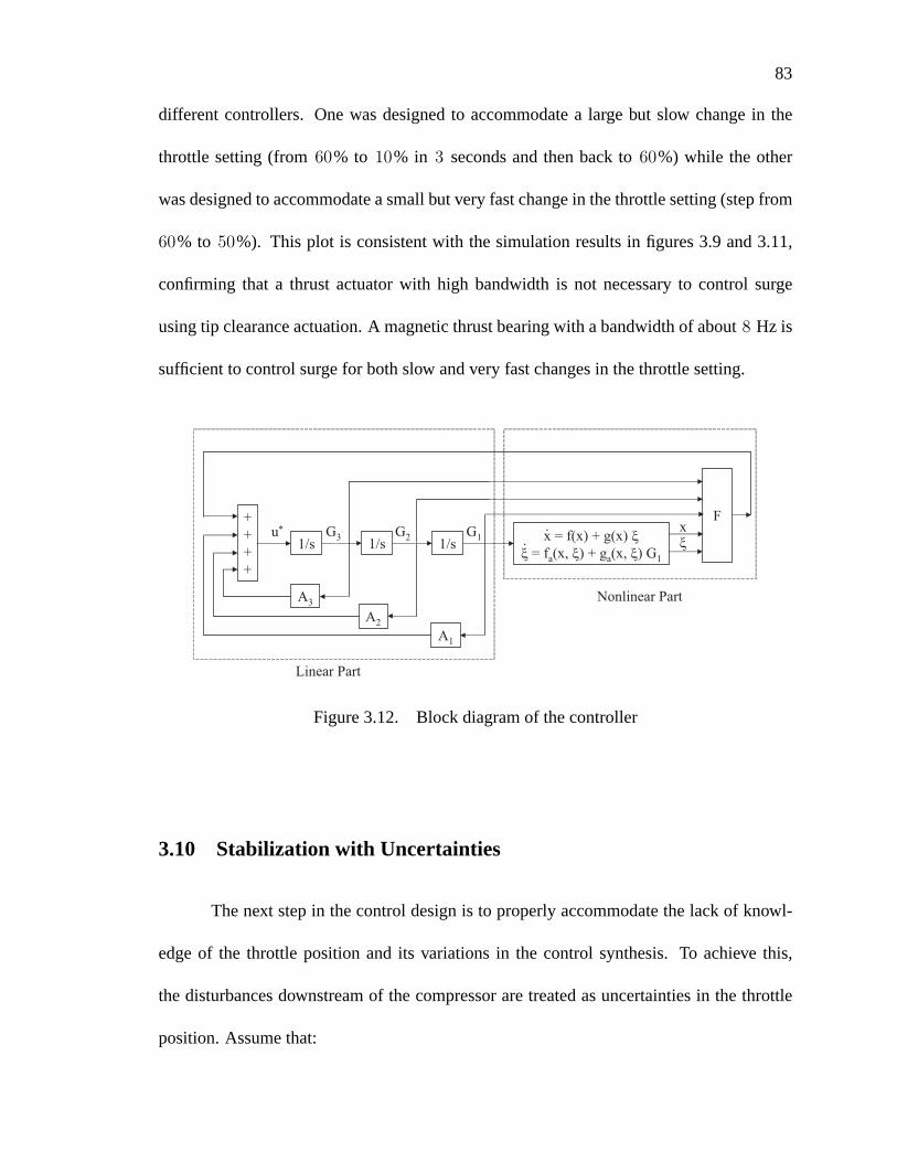
83

different controllers. One was designed to accommodate a large but slow change in the

throttle setting (from 60% to 10% in 3 seconds and then back to 60%) while the other

was designed to accommodate a small but very fast change in the throttle setting (step from

60% to 50%). This plot is consistent with the simulation results in figures 3.9 and 3.11,

confirming that a thrust actuator with high bandwidth is not necessary to control surge

using tip clearance actuation. A magnetic thrust bearing with a bandwidth of about 8 Hz is

sufficient to control surge for both slow and very fast changes in the throttle setting.

A3

A2A1

F

1/s 1/s 1/sG3 G2 G1u* x

ξ

++++

x = f(x) + g(x) ξξ = fa(x, ξ) + ga(x, ξ) G1

..

Linear Part

Nonlinear Part

Figure 3.12. Block diagram of the controller

3.10 Stabilization with Uncertainties

The next step in the control design is to properly accommodate the lack of knowl-

edge of the throttle position and its variations in the control synthesis. To achieve this,

the disturbances downstream of the compressor are treated as uncertainties in the throttle

position. Assume that:

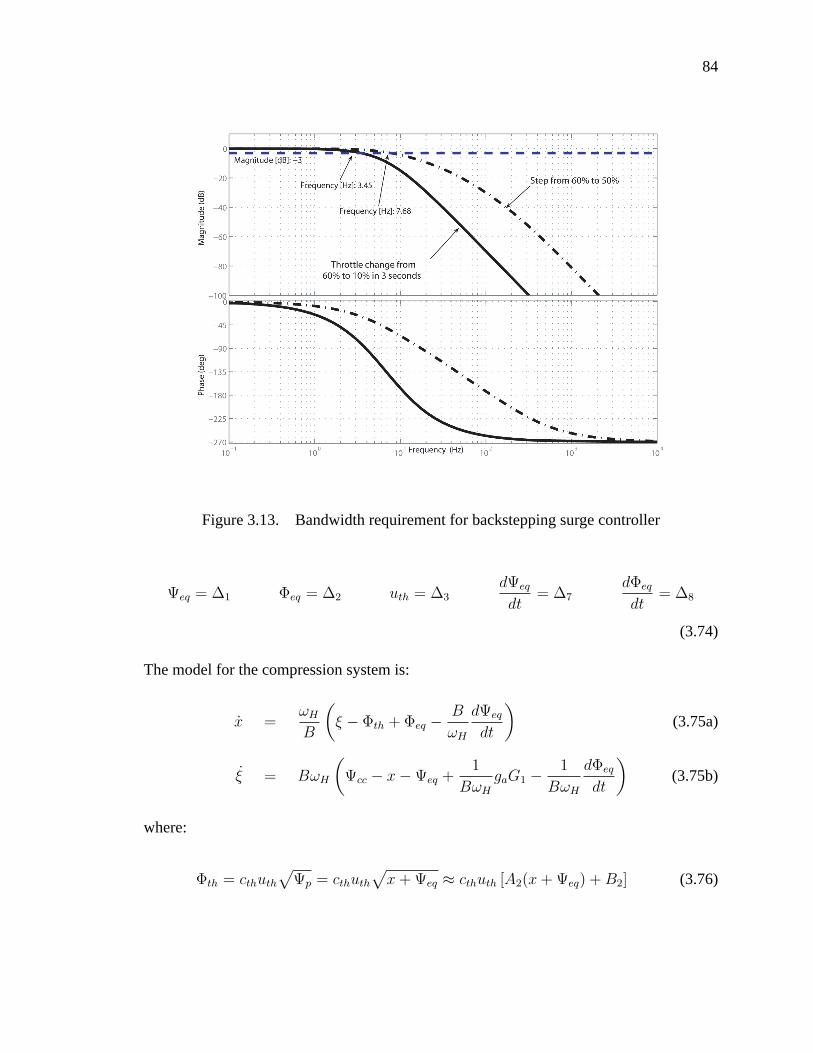
84

Figure 3.13. Bandwidth requirement for backstepping surge controller

Ψeq = ∆1 Φeq = ∆2 uth = ∆3dΨeq

dt= ∆7

dΦeq

dt= ∆8

(3.74)

The model for the compression system is:

x =ωH

B

(ξ − Φth + Φeq − B

ωH

dΨeq

dt

)(3.75a)

ξ = BωH

(Ψcc − x− Ψeq +

1

BωH

gaG1 − 1

BωH

dΦeq

dt

)(3.75b)

where:

Φth = cthuth

√Ψp = cthuth

√x+ Ψeq ≈ cthuth [A2(x+ Ψeq) +B2] (3.76)

85

This linearized model for the throttle mass flow rates very closely follows the orig-

inal square root function in the interested range of operation. Therefore (3.75a) becomes:

x =ωH

B

(ξ − cthuth [A2(x+ Ψeq) +B2] + Φeq − B

ωH

dΨeq

dt

)

Define ∆4 ≡ ∆3∆1 so that:

x =ωH

B

(ξ − cth(A2x+B2)∆3 − cthA2∆4 + ∆2 − B

ωH

∆7

)(3.77)

Equation (3.75b) can be rewritten in terms of the uncertainties as:

ξ = BωH

(Po1

12ρU2

[A1(ξ + ∆2)

3 +B1(ξ + ∆2)2 + C1(ξ + ∆2) +D − 1

]

−x− ∆1 +1

BωH

gaG1 − 1

BωH

∆8

)

Assign:

f2a(x, ξ) =Po1

12ρU2

(A1ξ

3 +B1ξ2 + C1ξ

)− x+Po1(D − 1)

12ρU2

(3.78)

∆5 = 3A1∆22 + 2B1∆2 (3.79)

∆6 = A1∆32 +B1∆

22 + C1∆2 (3.80)

With this, the system model including the throttle uncertainties becomes:

x =ωH

B

(ξ − cth(A2x+B2)∆3 − cthA2∆4 + ∆2 − B

ωH

∆7

)(3.81a)

ξ = BωH

(f2a(x, ξ) +

1

BωH

gaG1 +3Po1A1

12ρU2

ξ2∆2 +Po1

12ρU2

ξ∆5 +Po1

12ρU2

∆6

−∆1 − 1

BωH

∆8

)(3.81b)

To find the stabilizing controller, G1 , introduce:

86

V1(x) =B

2ωH

x2 (3.82)

The derivative of V1(x) is:

V1 = x

[ξ − cth(A2x+B2)∆3 − cthA2∆4 + ∆2 − B

ωH

∆7

](3.83)

Choose:

ξ = α1(x) = −σ1x− k1x

[1 + (cth(A2x+B2))

2 + (cthA2)2 +

(B

ωH

)2]

(3.84)

to produce:

V1 = −σ1x2 − xcth(A2x+B2)∆3 − k1x

2 (−cth(A2x+B2))2 − xcthA2∆4

−k1x2 (−cthA2)

2 + x∆2 − k1x2 − x

B

ωH

∆7 − k1x2

(−BωH

)2

(3.85)

Young’s Inequality [31]: If the constants p > 1 and q > 1 are such that (p −

1)(q − 1) = 1 , then for all ε > 0 and all (x, y) ∈ R2 we have

xy ≤ εp

p|x|p +

1

qεq|y|q (3.86)

Choosing p = q = 2 and ε2 = 2k , (3.86) becomes

xy ≤ kx2 +1

4ky2

→ xy − kx2 ≤ 1

4ky2 (3.87)

Rewrite (3.85):

V1 = −σ1x2 − xcth(A2x+B2)∆3 − k1x

2 (−cth(A2x+B2))2 − xcthA2∆4

−k1x2 (−cthA2)

2 + x∆2 − k1x2 − x

B

ωH

∆7 − k1x2

(−BωH

)2

87

V1 ≤ −σ1x2 − xcth(A2x+B2) ‖ ∆3 ‖∞ −k1x

2 (−cth(A2x+B2))2

−xcthA2 ‖ ∆4 ‖∞ −k1x2 (−cthA2)

2 + x ‖ ∆2 ‖∞ −k1x2

−x BωH

‖ ∆7 ‖∞ −k1x2

(−BωH

)2

by(3.87) V1 ≤ −σ1x2 +

‖ ∆3 ‖2∞

4k1

+‖ ∆4 ‖2

∞4k1

+‖ ∆2 ‖2

∞4k1

+‖ ∆7 ‖2

∞4k1

(3.88)

Define:

W1(x) = σ1x2 > 0 (3.89)

b1 =1

4k1

[‖ ∆3 ‖2∞ + ‖ ∆4 ‖2

∞ + ‖ ∆2 ‖2∞ + ‖ ∆7 ‖2

∞]

(3.90)

Therefore:

V1 ≤ −W1(x) + b1 (3.91)

In (3.91), it follows that V1 is negative whenever W1(x) > b1 . The radial unboundedness

of W1(x) combined with (3.88) implies that V1 is negative outside a compact set, which in

turns implies that x(t) and ξ(t) are globally uniformly bounded.

3.11 Backstepping with Uncertainties

The augmented system is:

x =ωH

B

(ξ − cth(A2x+B2)∆3 − cthA2∆4 + ∆2 − B

ωH

∆7

)

ξ = BωH

(f2a(x, ξ) +

1

BωH

gaG1 +3Po1A1

12ρU2

ξ2∆2 +Po1

12ρU2

ξ∆5 +Po1

12ρU2

∆6

−∆1 − 1

BωH

∆8

)

88

To find the stabilizing controller for the above system, define:

G0 = BωHf2a(x, ξ) + gaG1 (3.92)

so that the system model becomes:

x =ωH

B

(ξ − cth(A2x+B2)∆3 − cthA2∆4 + ∆2 − B

ωH

∆7

)(3.93a)

ξ = G0 +BωH

(3Po1A1

12ρU2

ξ2∆2 +Po1

12ρU2

ξ∆5 +Po1

12ρU2

∆6 − ∆1 − 1

BωH

∆8

)

(3.93b)

in which ξ is the control input that makes x = 0 the global asymptotic equilibrium of

(3.93a) and is calculated from (3.84). To find the control input G0 for the augmented

system (3.93), define:

V2 = V1 +1

2λ1BωH

[ξ − α1]2 (3.94)

Therefore:

V2 = x

[ξ − cth(A2x+B2)∆3 − cthA2∆4 + ∆2 − B

ωH

∆7

]

+1

λ1

[ξ − α1]

[1

BωH

ξ − 1

BωH

∂α1

∂xx

]

V2 ≤ −W1(x) + b1 +1

λ1

[ξ − α1]

[1

BωH

G0 + λ1x− 1

B2

∂α1

∂xξ +

3Po1A1

12ρU2

ξ2∆2

+Po1

12ρU2

ξ∆5 +Po1

12ρU2

∆6 − ∆1 − 1

BωH

∆8 +1

B2

∂α1

∂xcth(A2x+B2)∆3

+1

B2

∂α1

∂xcthA2∆4 − 1

B2

∂α1

∂x∆2 +

1

BωH

∂α1

∂x∆7

](3.95)

Choose:

89

1

BωH

G0 =1

BωH

α2(x, ξ) = −σ2[ξ − α1] − λ1x+1

B2

∂α1

∂xξ − k2

λ1

[ξ − α1]

[1

(−BωH)2

+

(3Po1A1

12ρU2

ξ2

)2

+

(Po1

12ρU2

ξ

)2

+

(Po1

12ρU2

)2

+ 1 +

(1

B2

∂α1

∂xcth(A2x+B2)

)2

+

(1

B2

∂α1

∂xcthA2

)2

+

(1

B2

∂α1

∂x

)2

+

(1

BωH

∂α1

∂x

)2]

(3.96)

Then:

V2≤−W1(x) + b1 − σ2

λ1

[ξ − α1]2 +

[ξ − α1]

λ1

3Po1A1

12ρU2

ξ2 ‖ ∆2 ‖∞

−k2

λ21

[ξ − α1]2

(3Po1A1

12ρU2

ξ2

)2

+[ξ − α1]

λ1

Po1

12ρU2

ξ ‖ ∆5 ‖∞

−k2

λ21

[ξ − α1]2

(Po1

12ρU2

ξ

)2

+[ξ − α1]

λ1

Po1

12ρU2

‖ ∆6 ‖∞

−k2

λ21

[ξ − α1]2

(Po1

12ρU2

)2

− [ξ − α1]

λ1

‖ ∆1 ‖∞ −k2

λ21

[ξ − α1]2 1

(BωH)2

− [ξ − α1]

λ1

‖ ∆8 ‖∞ −k2

λ21

[ξ − α1]2 +

[ξ − α1]

λ1

1

B2

∂α1

∂xcth(A2x+B2) ‖ ∆3 ‖∞

−k2

λ21

[ξ − α1]2

(1

B2

∂α1

∂xcth(A2x+B2)

)2

+[ξ − α1]

λ1

1

B2

∂α1

∂xcthA2 ‖ ∆4 ‖∞

−k2

λ21

[ξ − α1]2

(1

B2

∂α1

∂xcthA2

)2

− [ξ − α1]

λ1

1

B2

∂α1

∂x‖ ∆2 ‖∞

−k2

λ21

[ξ − α1]2

(−1

B2

∂α1

∂x

)2

+[ξ − α1]

λ1

1

BωH

∂α1

∂x‖ ∆7 ‖∞

−k2

λ21

[ξ − α1]2

(1

BωH

∂α1

∂x

)2

by(3.87) V2 ≤ −W1(x) + b1 − σ2

λ1

[ξ − α1]2 +

‖ ∆2 ‖2∞

4k2

+‖ ∆5 ‖2

∞4k2

+‖ ∆6 ‖2

∞4k2

+‖ ∆1 ‖2

∞4k2

+‖ ∆8 ‖2

∞4k2

+‖ ∆3 ‖2

∞4k2

+‖ ∆4 ‖2

∞4k2

+‖ ∆2 ‖2

∞4k2

+‖ ∆7 ‖2

∞4k2

90

Define:

W2(x, ξ) =σ2

λ1

[ξ − α1]2 (3.97)

b2 =1

4k2

[‖ ∆2 ‖2∞ + ‖ ∆5 ‖2

∞ + ‖ ∆6 ‖2∞ + ‖ ∆1 ‖2

∞ + ‖ ∆8 ‖2∞

+ ‖ ∆3 ‖2∞ + ‖ ∆4 ‖2

∞ + ‖ ∆2 ‖2∞ + ‖ ∆7 ‖2

∞]

(3.98)

to produce, finally:

V2 ≤ −W1(x) + b1 −W2(x, ξ) + b2 (3.99)

so that V2 is negative whenever:

W1(x) +W2(x, ξ) > b1 + b2 (3.100)

This implies that V2 is negative outside a compact set determined by b1 and b2 which are

set by the bounds in the uncertainties in the throttle settings. This in turn implies that x(t)

and ξ(t) are globally uniformly bounded.

Using (3.92) the tip clearance modulation, G1 , becomes:

G1 = α20 =1

ga

(α2 −BωHf2a) (3.101)


Simulation results for the derived backstepping controller are shown in Fig. 3.14.

Results are shown for the same changes in the throttle opening as in the previous cases

(from 60% opening to 10% opening -where the compressor would be operating in deep

surge if the controller was not activated- in 3 seconds and opens back to 60% opening in 3

91

seconds). The controller is designed without any knowledge of the throttle valve position

and its changes with time.

The compressor characteristic curve and the transient response of the system are

plotted in Fig. 3.14-b,c and d. Since the controller was designed without having any knowl-

edge of the throttle position and therefore system’s equilibrium point, there is an offset

from the steady state compressor characteristic curve in the state trajectories and the final

impeller location as shown in Fig. 3.14-c, d, and e.

[%]

Figure 3.14. Transient response and control requirement for backstepping with uncertain-

ties

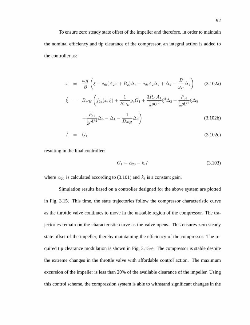
92

To ensure zero steady state offset of the impeller and therefore, in order to maintain

the nominal efficiency and tip clearance of the compressor, an integral action is added to

the controller as:

x =ωH

B

(ξ − cth(A2x+B2)∆3 − cthA2∆4 + ∆2 − B

ωH

∆7

)(3.102a)

ξ = BωH

(f2a(x, ξ) +

1

BωH

gaG1 +3Po1A1

12ρU2

ξ2∆2 +Po1

12ρU2

ξ∆5

+Po1

12ρU2

∆6 − ∆1 − 1

BωH

∆8

)(3.102b)

I = G1 (3.102c)

resulting in the final controller:

G1 = α20 − kiI (3.103)

where α20 is calculated according to (3.101) and ki is a constant gain.

Simulation results based on a controller designed for the above system are plotted

in Fig. 3.15. This time, the state trajectories follow the compressor characteristic curve

as the throttle valve continues to move in the unstable region of the compressor. The tra-

jectories remain on the characteristic curve as the valve opens. This ensures zero steady

state offset of the impeller, thereby maintaining the efficiency of the compressor. The re-

quired tip clearance modulation is shown in Fig. 3.15-e. The compressor is stable despite

the extreme changes in the throttle valve with affordable control action. The maximum

excursion of the impeller is less than 20% of the available clearance of the impeller. Using

this control scheme, the compression system is able to withstand significant changes in the

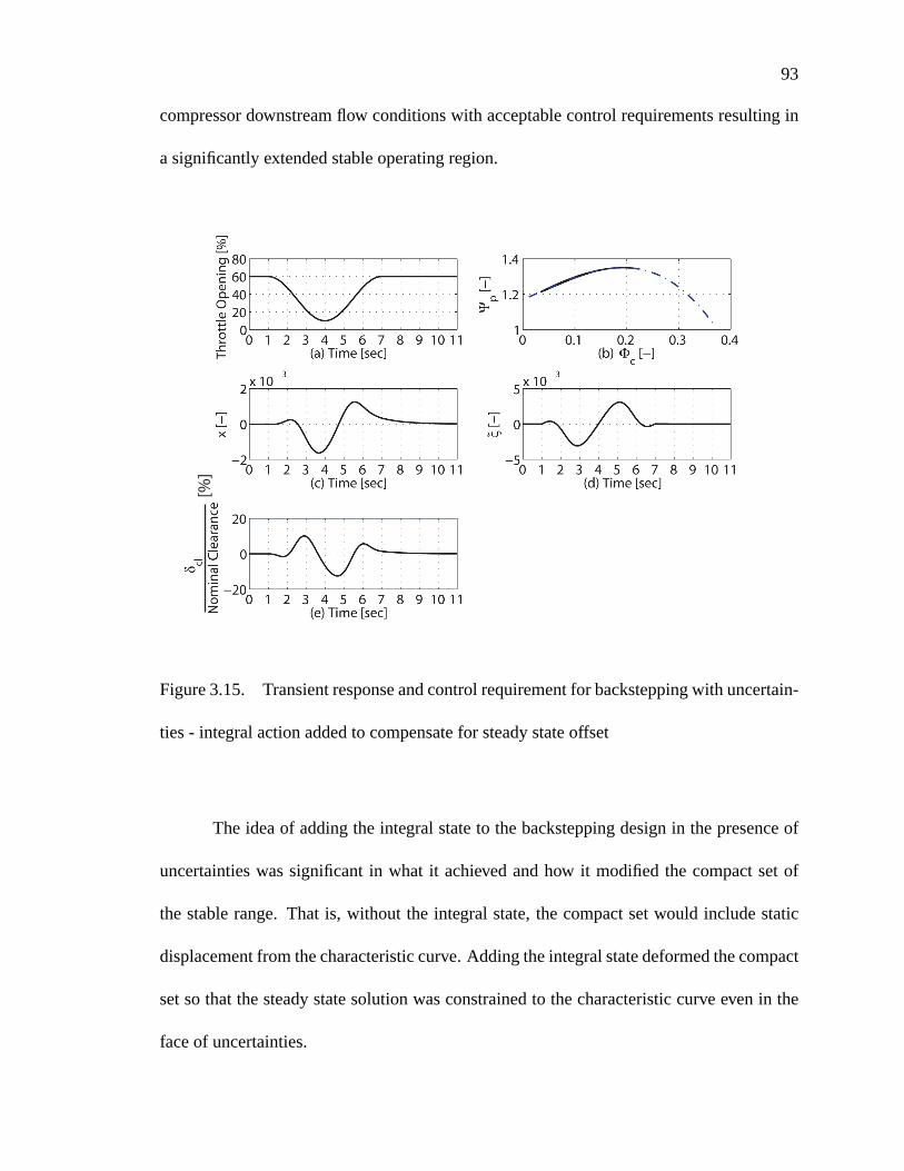
93

compressor downstream flow conditions with acceptable control requirements resulting in

a significantly extended stable operating region.

[%]

Figure 3.15. Transient response and control requirement for backstepping with uncertain-

ties - integral action added to compensate for steady state offset

The idea of adding the integral state to the backstepping design in the presence of

uncertainties was significant in what it achieved and how it modified the compact set of

the stable range. That is, without the integral state, the compact set would include static

displacement from the characteristic curve. Adding the integral state deformed the compact

set so that the steady state solution was constrained to the characteristic curve even in the

face of uncertainties.

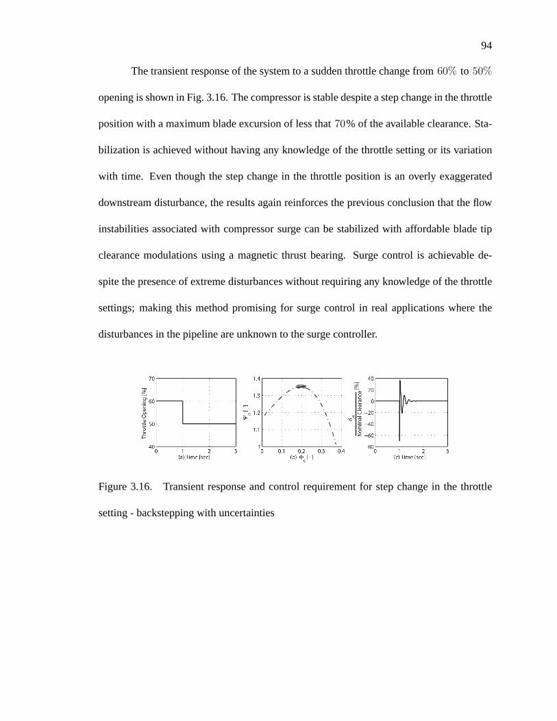
94

The transient response of the system to a sudden throttle change from 60% to 50%

opening is shown in Fig. 3.16. The compressor is stable despite a step change in the throttle

position with a maximum blade excursion of less that 70% of the available clearance. Sta-

bilization is achieved without having any knowledge of the throttle setting or its variation

with time. Even though the step change in the throttle position is an overly exaggerated

downstream disturbance, the results again reinforces the previous conclusion that the flow

instabilities associated with compressor surge can be stabilized with affordable blade tip

clearance modulations using a magnetic thrust bearing. Surge control is achievable de-

spite the presence of extreme disturbances without requiring any knowledge of the throttle

settings; making this method promising for surge control in real applications where the

disturbances in the pipeline are unknown to the surge controller.

[%]

Figure 3.16. Transient response and control requirement for step change in the throttle

setting - backstepping with uncertainties

95

3.12 Backstepping with Uncertainties and Bandwidth Limitations

To establish the thrust bearing bandwidth requirement in the presence of throttle un-

certainties, the thrust bearing dynamics should be included in the control synthesis. Adding

the dynamics of the thrust bearing as a chain of integrators to the system with uncertainties

enormously complicates the algebra associated with the backstepping design. Given the

level of algebraic difficulty added to the control design with each integrator, the author was

not able to establish the actual actuator bandwidth requirement in the presence of throttle

uncertainties.

However, an upper bound on the required actuator bandwidth can be estimated by

modeling the thrust bearing as a low pass filter and passing the control signal resulting

from the backstepping design with uncertainties through this low pass filter(as was pre-

viously discussed in Section 3.2.1). Figure 3.17 shows the simulation result from such

a controller. The thrust bearing was modeled as a third–order low pass butterworth filter

and the control signal from (3.101) was passed through this filter to represent the physical

limitation of the actual hardware. The simulation results show that a bandwidth of 80 Hz

is required to stabilize compressor surge for the same changes in the throttle setting as in

the previous simulations. Since the thrust bearing is not included in the control synthesis,

the limitations of the actuator are not considered in the control design. This tends to in-

crease the bandwidth request from the actuator to 80 Hz comparing to less than 10 Hz in

Section 3.9. Adding the thrust bearing dynamics in the control synthesis is expected to re-

duce this bandwidth requirement for surge control in the presence of throttle uncertainties.

However, this is something that can be the focus of future research.

96

0 2 4 6 80

20406080

Thro

ttle

Op

enin

g [%

](a) Time [sec]

0 0.1 0.2 0.3 0.41

1.2

1.4

Ψp [−

]

(b) Φc

[−]

0 5 10−5

0

5 x 10−3

x[−

]

(c) Time [sec]0 5 10

−5

0

5 x 10−3

ξ[−

]

(d) Time [sec]

0 5 10−20

0

20

δ clN

om

inal

Cle

aran

ce

(e) Time [sec]

[%]

Figure 3.17. Transient response for backstepping with uncertainties - thrust bearing mod-

eled as a low pass filter

3.13 Conclusion

The goal of the research presented in this chapter was to develop a new method for

controlling surge in single stage unshrouded centrifugal compressors which is capable of

substantially mitigating flow instabilities using the magnetic thrust bearing to modulate the

impeller tip clearance. Different control methodologies were considered for this purpose.

A mass flow feedback was originally proposed which was able to significantly increase the

stable operating range of the compressor. However, the stability condition for mass flow

feedback was developed assuming infinite actuator bandwidth, constant throttle position

and no uncertainties in the throttle settings.

97

The control objective was to force the state trajectories to follow the steady state

compressor characteristic curve. The sliding mode control method seemed to be the perfect

candidate to achieve such a goal. However, problems arose because of the singularity of the

controller at the peak of the compressor characteristic curve and the algebraic difficulties

associated with putting the system into the cascade of integrators canonical form required

by sliding mode formulation.

The singularity problem at the peak of the compressor characteristic curve is not an

issue with the backstepping method. Backstepping also permits inclusion of the uncertain-

ties in the throttle setting in the control synthesis. A backstepping controller was designed

with the objective that system trajectories remain on the compressor characteristic curve in

the presence of disturbances downstream of the compressor which are modeled as changes

in the throttle opening. This ensured zero steady state offset of the impeller, maintaining

the efficiency of the compressor. Results from the simulation of the nonlinear model for

a single stage high speed centrifugal compressor showed that, using backstepping control,

mass flow and pressure oscillations associated with compressor surge were very effectively

suppressed and the stable operating range of the compressor was increased significantly.

Throttle changes producing a reduction in mass flow rate from 60% to 10% in 3 seconds

were readily accommodated by the controller with very acceptable impeller excursions.

The thrust bearing dynamics were included in the synthesis of the backstepping controller

and showed modest bandwidth requirement for this control method which makes it more

attractive for industrial applications.

The ultimate goal of the application of backstepping to this problem was to properly

accommodate lack of knowledge of throttle position in design of the control. Simulation

98

results showed that the compression system can be stabilized in the presence of downstream

disturbances with acceptable impeller tip clearance modulation. However, this would result

in a static offset from the steady state compressor characteristic curve. An integral state

was successfully added to the backstepping design to compensate for this static offset and

to force the state trajectories follow the steady state compressor characteristic. The notion

of adding auxiliary integral states to the backstepping problem with uncertainties in order

to deform the unstable compact set characterizing the residual limit cycles appears to be

new to the literature. The added flexibility that this introduces: being able to avoid certain

undesirable directions in the limit cycles can substantially improve the performance of

these controllers, as evidenced in the present example.

99

CHAPTER 4

EXPERIMENTAL FACILITY AND SYSTEM

IDENTIFICATION

A test facility with magnetic bearings was designed and constructed to enable mea-

surement of off-design impeller loads and to support experimental investigation of the pro-

posed surge control method. This chapter provides an overview of the test rig and its

capabilities.

4.1 Test Rig Overview

The test rig has six main mechanical sections: 1) Compressor, 2) Test section,

3) Motor and its cooling system, 4) Flexible coupling 5) Inlet and discharge ducting and

100

6) Data acquisition system. The schematic of the test facility and its final assembly are

shown in Fig. 4.1.

Impeller Test SectionMotor

Baseplate

MotorTest Section

Compressor

Coupling

Figure 4.1. Assembly of the compressor test facility

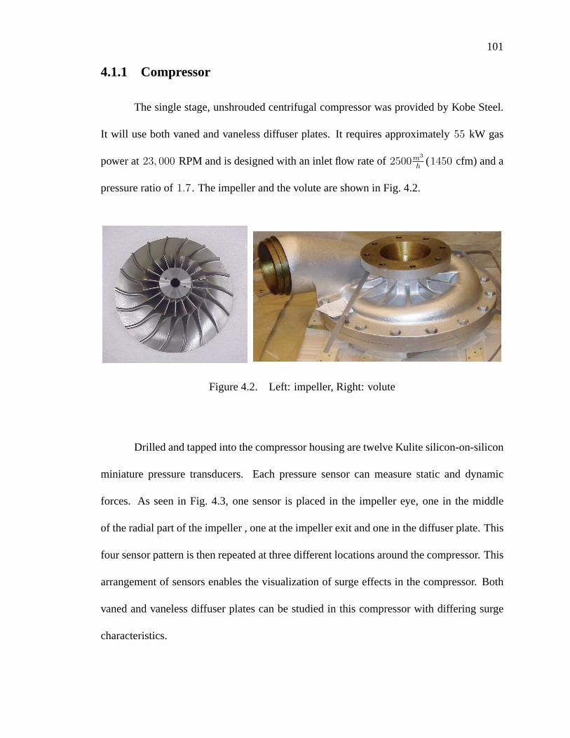
101

4.1.1 Compressor

The single stage, unshrouded centrifugal compressor was provided by Kobe Steel.

It will use both vaned and vaneless diffuser plates. It requires approximately 55 kW gas

power at 23, 000 RPM and is designed with an inlet flow rate of 2500m3

h(1450 cfm) and a

pressure ratio of 1.7 . The impeller and the volute are shown in Fig. 4.2.

Figure 4.2. Left: impeller, Right: volute

Drilled and tapped into the compressor housing are twelve Kulite silicon-on-silicon

miniature pressure transducers. Each pressure sensor can measure static and dynamic

forces. As seen in Fig. 4.3, one sensor is placed in the impeller eye, one in the middle

of the radial part of the impeller , one at the impeller exit and one in the diffuser plate. This

four sensor pattern is then repeated at three different locations around the compressor. This

arrangement of sensors enables the visualization of surge effects in the compressor. Both

vaned and vaneless diffuser plates can be studied in this compressor with differing surge

characteristics.

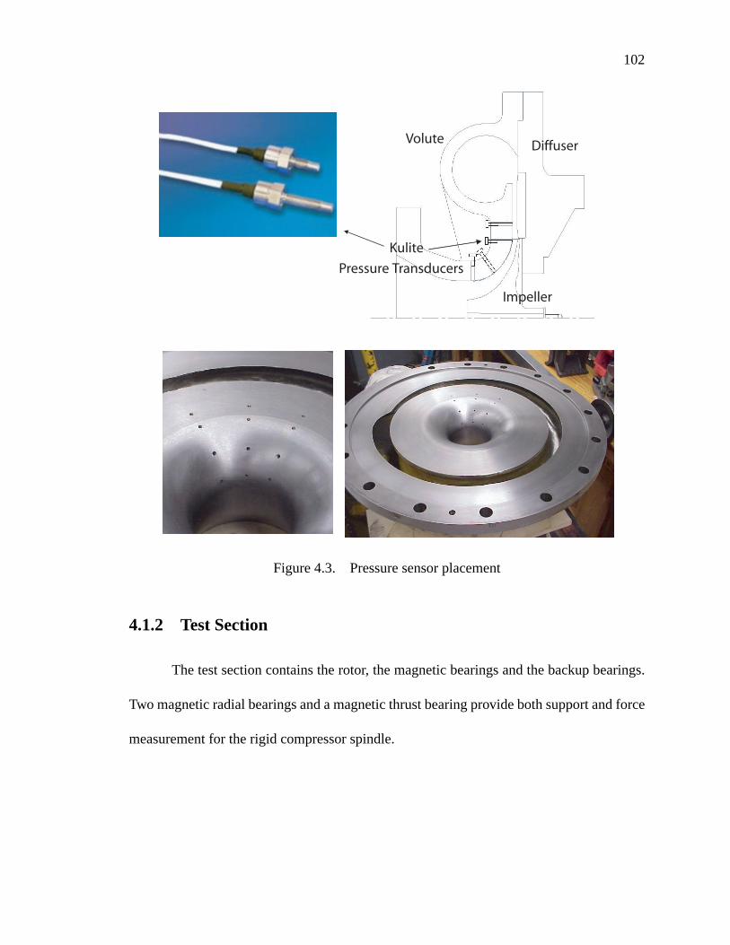
102

Volute

Impeller

Diffuser

Kulite

Pressure Transducers

Figure 4.3. Pressure sensor placement

4.1.2 Test Section

The test section contains the rotor, the magnetic bearings and the backup bearings.

Two magnetic radial bearings and a magnetic thrust bearing provide both support and force

measurement for the rigid compressor spindle.

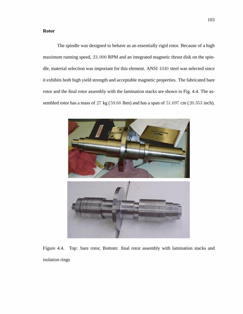
103

Rotor

The spindle was designed to behave as an essentially rigid rotor. Because of a high

maximum running speed, 23, 000 RPM and an integrated magnetic thrust disk on the spin-

dle, material selection was important for this element. ANSI 4340 steel was selected since

it exhibits both high yield strength and acceptable magnetic properties. The fabricated bare

rotor and the final rotor assembly with the lamination stacks are shown in Fig. 4.4. The as-

sembled rotor has a mass of 27 kg (59.68 lbm) and has a span of 51.697 cm (20.353 inch).

Figure 4.4. Top: bare rotor, Bottom: final rotor assembly with lamination stacks and

isolation rings

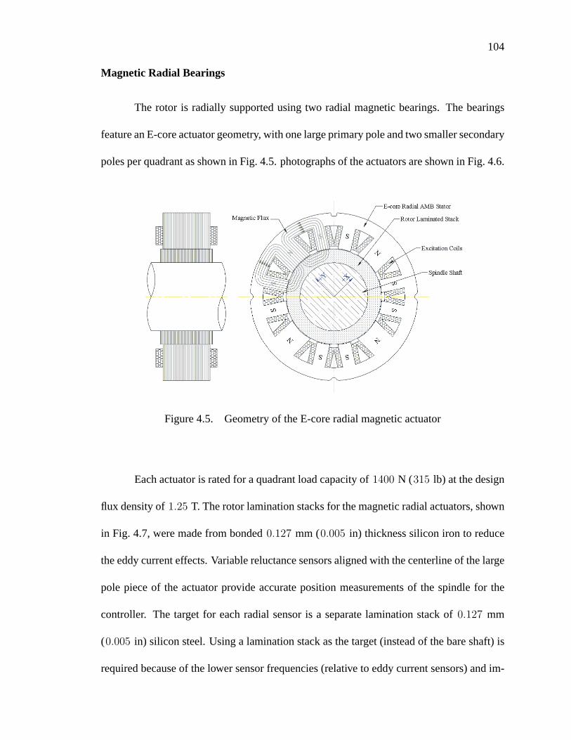
104

Magnetic Radial Bearings

The rotor is radially supported using two radial magnetic bearings. The bearings

feature an E-core actuator geometry, with one large primary pole and two smaller secondary

poles per quadrant as shown in Fig. 4.5. photographs of the actuators are shown in Fig. 4.6.

Figure 4.5. Geometry of the E-core radial magnetic actuator

Each actuator is rated for a quadrant load capacity of 1400 N (315 lb) at the design

flux density of 1.25 T. The rotor lamination stacks for the magnetic radial actuators, shown

in Fig. 4.7, were made from bonded 0.127 mm (0.005 in) thickness silicon iron to reduce

the eddy current effects. Variable reluctance sensors aligned with the centerline of the large

pole piece of the actuator provide accurate position measurements of the spindle for the

controller. The target for each radial sensor is a separate lamination stack of 0.127 mm

(0.005 in) silicon steel. Using a lamination stack as the target (instead of the bare shaft) is

required because of the lower sensor frequencies (relative to eddy current sensors) and im-

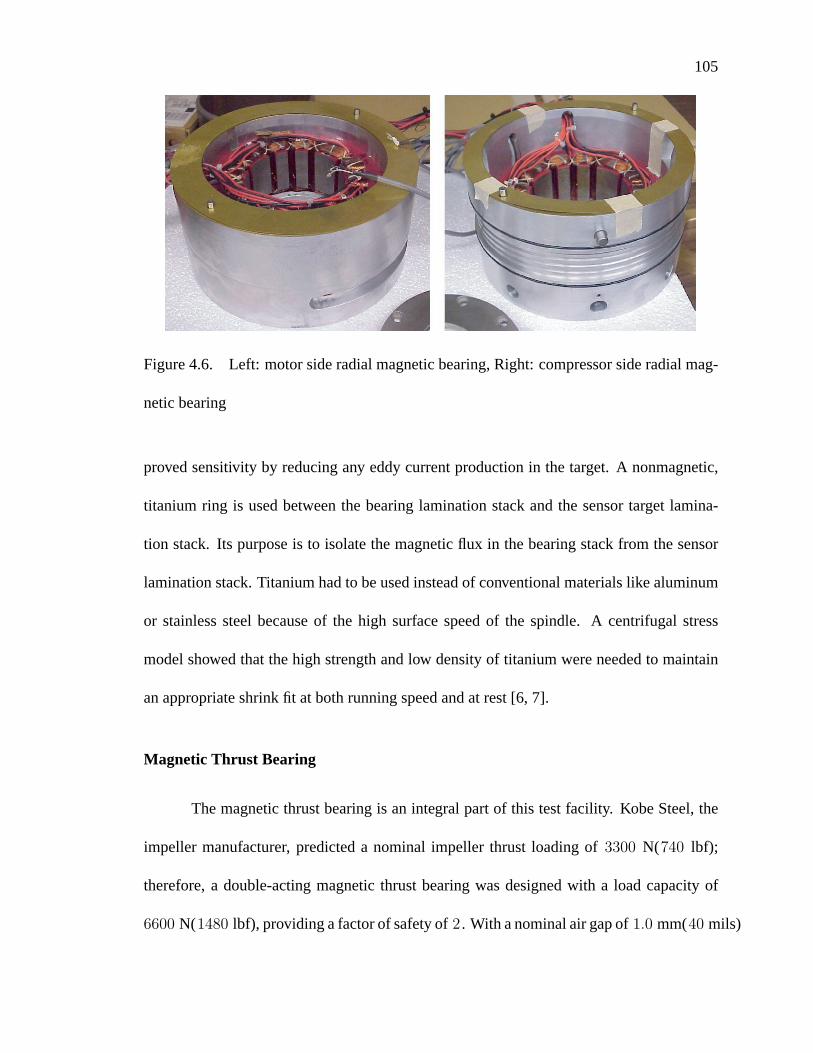
105

Figure 4.6. Left: motor side radial magnetic bearing, Right: compressor side radial mag-

netic bearing

proved sensitivity by reducing any eddy current production in the target. A nonmagnetic,

titanium ring is used between the bearing lamination stack and the sensor target lamina-

tion stack. Its purpose is to isolate the magnetic flux in the bearing stack from the sensor

lamination stack. Titanium had to be used instead of conventional materials like aluminum

or stainless steel because of the high surface speed of the spindle. A centrifugal stress

model showed that the high strength and low density of titanium were needed to maintain

an appropriate shrink fit at both running speed and at rest [6, 7].

Magnetic Thrust Bearing

The magnetic thrust bearing is an integral part of this test facility. Kobe Steel, the

impeller manufacturer, predicted a nominal impeller thrust loading of 3300 N(740 lbf);

therefore, a double-acting magnetic thrust bearing was designed with a load capacity of

6600 N(1480 lbf), providing a factor of safety of 2 . With a nominal air gap of 1.0 mm(40 mils)

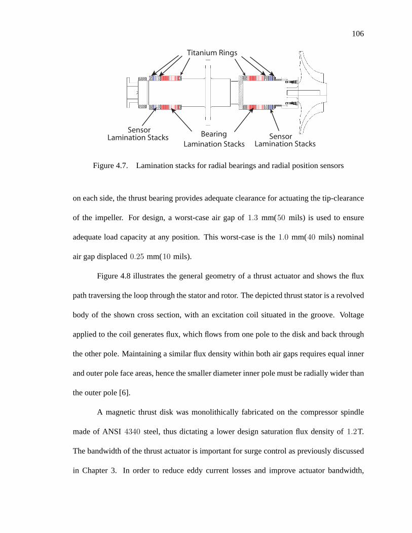
106

BearingSensorLamination Stacks

Lamination Stacks

Titanium Rings

Lamination StacksSensor

Figure 4.7. Lamination stacks for radial bearings and radial position sensors

on each side, the thrust bearing provides adequate clearance for actuating the tip-clearance

of the impeller. For design, a worst-case air gap of 1.3 mm(50 mils) is used to ensure

adequate load capacity at any position. This worst-case is the 1.0 mm(40 mils) nominal

air gap displaced 0.25 mm(10 mils).

Figure 4.8 illustrates the general geometry of a thrust actuator and shows the flux

path traversing the loop through the stator and rotor. The depicted thrust stator is a revolved

body of the shown cross section, with an excitation coil situated in the groove. Voltage

applied to the coil generates flux, which flows from one pole to the disk and back through

the other pole. Maintaining a similar flux density within both air gaps requires equal inner

and outer pole face areas, hence the smaller diameter inner pole must be radially wider than

the outer pole [6].

A magnetic thrust disk was monolithically fabricated on the compressor spindle

made of ANSI 4340 steel, thus dictating a lower design saturation flux density of 1.2T.

The bandwidth of the thrust actuator is important for surge control as previously discussed

in Chapter 3. In order to reduce eddy current losses and improve actuator bandwidth,

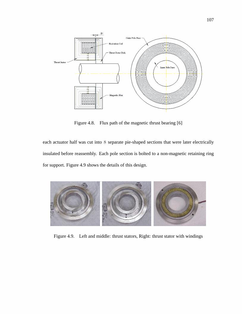
107

Figure 4.8. Flux path of the magnetic thrust bearing [6]

each actuator half was cut into 8 separate pie-shaped sections that were later electrically

insulated before reassembly. Each pole section is bolted to a non-magnetic retaining ring

for support. Figure 4.9 shows the details of this design.

Figure 4.9. Left and middle: thrust stators, Right: thrust stator with windings

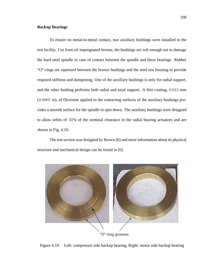
108

Backup Bearings

To ensure no metal-to-metal contact, two auxiliary bushings were installed in the

test facility. Cut from oil impregnated bronze, the bushings are soft enough not to damage

the hard steel spindle in case of contact between the spindle and these bearings. Rubber

“O”-rings are squeezed between the bronze bushings and the steel test housing to provide

required stiffness and dampening. One of the auxiliary bushings is only for radial support,

and the other bushing performs both radial and axial support. A thin coating, 0.013 mm

(0.0005 in), of Dicronite applied to the contacting surfaces of the auxiliary bushings pro-

vides a smooth surface for the spindle to spin down. The auxiliary bushings were designed

to allow orbits of 50% of the nominal clearance in the radial bearing actuators and are

shown in Fig. 4.10.

The test section was designed by Brown [6] and more information about its physical

structure and mechanical design can be found in [6].

“O”-ring grooves

Figure 4.10. Left: compressor side backup bearing, Right: motor side backup bearing

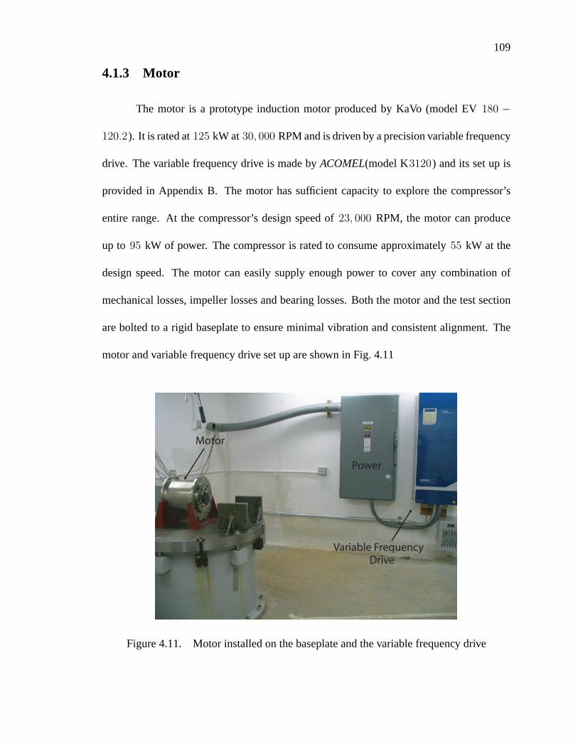
109

4.1.3 Motor

The motor is a prototype induction motor produced by KaVo (model EV 180 −

120.2). It is rated at 125 kW at 30, 000 RPM and is driven by a precision variable frequency

drive. The variable frequency drive is made by ACOMEL(model K3120) and its set up is

provided in Appendix B. The motor has sufficient capacity to explore the compressor’s

entire range. At the compressor’s design speed of 23, 000 RPM, the motor can produce

up to 95 kW of power. The compressor is rated to consume approximately 55 kW at the

design speed. The motor can easily supply enough power to cover any combination of

mechanical losses, impeller losses and bearing losses. Both the motor and the test section

are bolted to a rigid baseplate to ensure minimal vibration and consistent alignment. The

motor and variable frequency drive set up are shown in Fig. 4.11

Motor

Variable FrequencyDrive

Power

Figure 4.11. Motor installed on the baseplate and the variable frequency drive

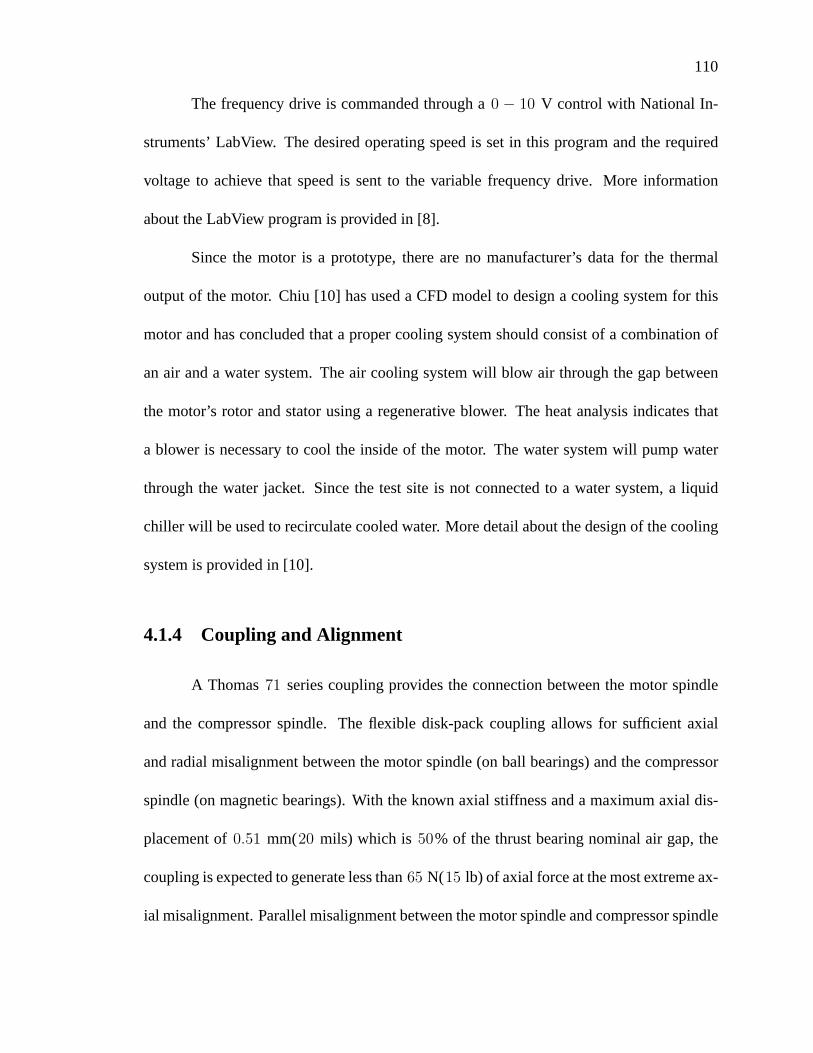
110

The frequency drive is commanded through a 0 − 10 V control with National In-

struments’ LabView. The desired operating speed is set in this program and the required

voltage to achieve that speed is sent to the variable frequency drive. More information

about the LabView program is provided in [8].

Since the motor is a prototype, there are no manufacturer’s data for the thermal

output of the motor. Chiu [10] has used a CFD model to design a cooling system for this

motor and has concluded that a proper cooling system should consist of a combination of

an air and a water system. The air cooling system will blow air through the gap between

the motor’s rotor and stator using a regenerative blower. The heat analysis indicates that

a blower is necessary to cool the inside of the motor. The water system will pump water

through the water jacket. Since the test site is not connected to a water system, a liquid

chiller will be used to recirculate cooled water. More detail about the design of the cooling

system is provided in [10].

4.1.4 Coupling and Alignment

A Thomas 71 series coupling provides the connection between the motor spindle

and the compressor spindle. The flexible disk-pack coupling allows for sufficient axial

and radial misalignment between the motor spindle (on ball bearings) and the compressor

spindle (on magnetic bearings). With the known axial stiffness and a maximum axial dis-

placement of 0.51 mm(20 mils) which is 50% of the thrust bearing nominal air gap, the

coupling is expected to generate less than 65 N(15 lb) of axial force at the most extreme ax-

ial misalignment. Parallel misalignment between the motor spindle and compressor spindle

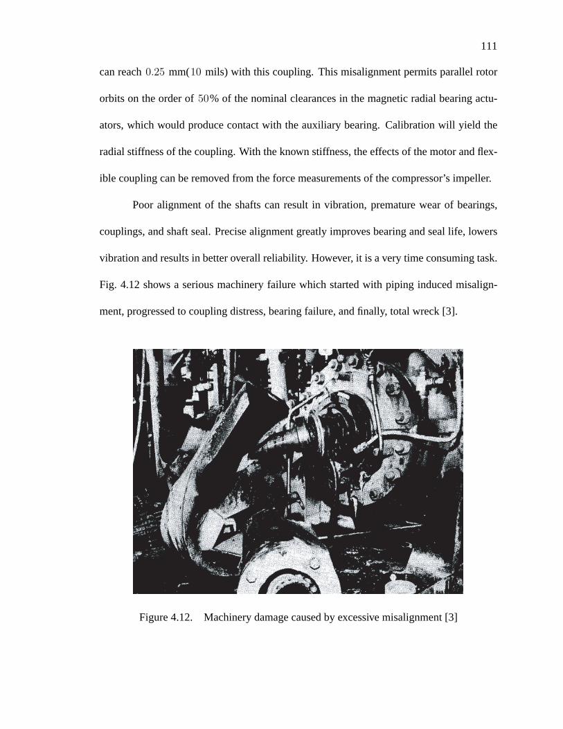
111

can reach 0.25 mm(10 mils) with this coupling. This misalignment permits parallel rotor

orbits on the order of 50% of the nominal clearances in the magnetic radial bearing actu-

ators, which would produce contact with the auxiliary bearing. Calibration will yield the

radial stiffness of the coupling. With the known stiffness, the effects of the motor and flex-

ible coupling can be removed from the force measurements of the compressor’s impeller.

Poor alignment of the shafts can result in vibration, premature wear of bearings,

couplings, and shaft seal. Precise alignment greatly improves bearing and seal life, lowers

vibration and results in better overall reliability. However, it is a very time consuming task.

Fig. 4.12 shows a serious machinery failure which started with piping induced misalign-

ment, progressed to coupling distress, bearing failure, and finally, total wreck [3].

Figure 4.12. Machinery damage caused by excessive misalignment [3]

112

The shafts can be precisely aligned using laser alignment techniques. Because of

the lack of space for mounting equipment, laser alignment can not be implemented on this

test rig. The Rim-and-Face method was used to align the motor shaft with the compressor

shaft. Acceptable shaft alignment on the order of less than 2 mils can be achieved using the

Rim-and-Face method. In this method, two dial indicators are used as shown in Fig. 4.14.

The alignment bracket is firmly attached to one shaft. One indicator reads the face of

the hub and the other indicator reads the rim of the hub. The indicators are zeroed at 12

o’clock. Both shafts and the bracket arrangement are slowly rotated through 90 degree

intervals stopping at 3 , 6 and 9 o’clock positions. To cancel out the effects of runout,

both shafts should be rotated at the same time. The procedure is repeated two times to

verify the set of readings. Shims are added to the various feet of the movable machine (the

motor in this case) to compensate for the face and rim misalignments. The schematic of the

Rim-and-Face alignment method and the shafts setups are shown in Figures 4.14 and 4.13.

Details about how to calculate each foot’s shim adjustment are provided in [3, 47].

Due to an unacceptable runout on the motor hub in this test rig (7 mils), it is not

possible to align the shafts to an acceptable level. It is recommended that the motor hub

be removed using a bearing puller and be reinstalled on the motor shaft after checking the

hub and shaft runouts. The final runout on the shaft and hub assembly should be less than

2 mils before starting the Rim-and-Face alignment procedure.

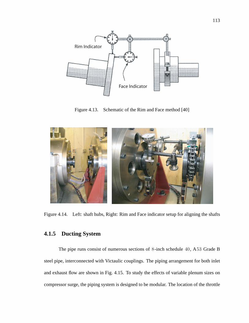
113

Rim Indicator

Face Indicator

Figure 4.13. Schematic of the Rim and Face method [40]

Figure 4.14. Left: shaft hubs, Right: Rim and Face indicator setup for aligning the shafts

4.1.5 Ducting System

The pipe runs consist of numerous sections of 8-inch schedule 40 , A53 Grade B

steel pipe, interconnected with Victaulic couplings. The piping arrangement for both inlet

and exhaust flow are shown in Fig. 4.15. To study the effects of variable plenum sizes on

compressor surge, the piping system is designed to be modular. The location of the throttle

114

valve can vary within the pipe run to change the plenum size. Minimum straight runs for

the inlet and exhaust are chosen according to Power Test Code (PTC) [1] to ensure reliable

measurements.

Figure 4.15. Layout of the piping arrangement

115

4.1.6 Data Acquisition System

Major data acquisition is performed using LabView. Two high speed data acquisi-

tion (DAQ) cards, National Instruments PCI-6052 and PCI-6071 , are used in conjunction

with NI’s signal processing cards. The Kulite pressure transducers are measured using NI’s

SCXI-1520 which incorporates a full-bridge with internal 0 − 10 V excitation. Numerous

T-type thermocouples are measured with NI’s SCXI-1102 which features an internal 2 Hz

low pass filter. Where possible, instrumentation is installed in accordance with the 1997

version of the Power Test Code (PTC). Proper sampling rates were set for each instrument

to capture all relevant information. Pressure sensors are sampled at 5 kHz, position sensors

at 3 kHz, thermocouples at 10 Hz. The user interface for the LabView program is shown

in Fig. 4.16. More information about this program is provided in [8].

4.2 Rotor Identification

A first step towards identifying a rotor/bearing system is measuring the natural fre-

quencies of the rotor. The rotor is designed for a running speed of 23000 RPM (383 Hz).

If the first bending mode occurs at a frequency higher than the design speed, then the rotor

will not undergo violent resonance related vibration while getting up to speed.

4.2.1 Impact Test

A rotor impact test, also known as ring test is the common tool for identifying the

natural frequencies of a rotor [27]. Ideally, the rotor should be in free-free support while

performing the impact test. This means that the rotor should be floating in the air. Since

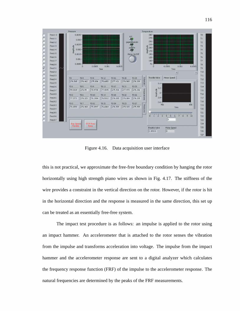
116

Figure 4.16. Data acquisition user interface

this is not practical, we approximate the free-free boundary condition by hanging the rotor

horizontally using high strength piano wires as shown in Fig. 4.17. The stiffness of the

wire provides a constraint in the vertical direction on the rotor. However, if the rotor is hit

in the horizontal direction and the response is measured in the same direction, this set up

can be treated as an essentially free-free system.

The impact test procedure is as follows: an impulse is applied to the rotor using

an impact hammer. An accelerometer that is attached to the rotor senses the vibration

from the impulse and transforms acceleration into voltage. The impulse from the impact

hammer and the accelerometer response are sent to a digital analyzer which calculates

the frequency response function (FRF) of the impulse to the accelerometer response. The

natural frequencies are determined by the peaks of the FRF measurements.

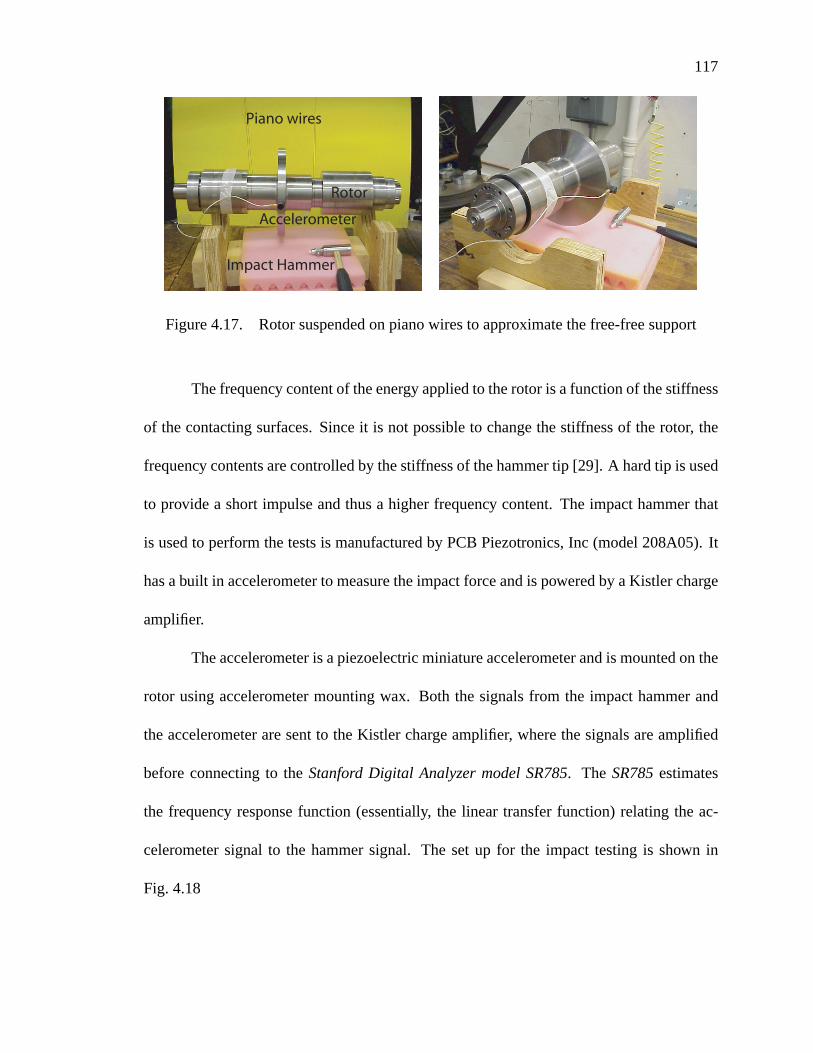
117

Impact Hammer

Rotor

Accelerometer

Piano wires

Figure 4.17. Rotor suspended on piano wires to approximate the free-free support

The frequency content of the energy applied to the rotor is a function of the stiffness

of the contacting surfaces. Since it is not possible to change the stiffness of the rotor, the

frequency contents are controlled by the stiffness of the hammer tip [29]. A hard tip is used

to provide a short impulse and thus a higher frequency content. The impact hammer that

is used to perform the tests is manufactured by PCB Piezotronics, Inc (model 208A05). It

has a built in accelerometer to measure the impact force and is powered by a Kistler charge

amplifier.

The accelerometer is a piezoelectric miniature accelerometer and is mounted on the

rotor using accelerometer mounting wax. Both the signals from the impact hammer and

the accelerometer are sent to the Kistler charge amplifier, where the signals are amplified

before connecting to the Stanford Digital Analyzer model SR785. The SR785 estimates

the frequency response function (essentially, the linear transfer function) relating the ac-

celerometer signal to the hammer signal. The set up for the impact testing is shown in

Fig. 4.18

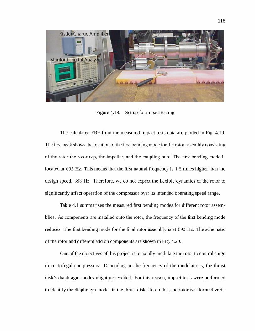
118

Stanford Digital Analyzer

Kistler Charge Amplifier

Figure 4.18. Set up for impact testing

The calculated FRF from the measured impact tests data are plotted in Fig. 4.19.

The first peak shows the location of the first bending mode for the rotor assembly consisting

of the rotor the rotor cap, the impeller, and the coupling hub. The first bending mode is

located at 692 Hz. This means that the first natural frequency is 1.8 times higher than the

design speed, 383 Hz. Therefore, we do not expect the flexible dynamics of the rotor to

significantly affect operation of the compressor over its intended operating speed range.

Table 4.1 summarizes the measured first bending modes for different rotor assem-

blies. As components are installed onto the rotor, the frequency of the first bending mode

reduces. The first bending mode for the final rotor assembly is at 692 Hz. The schematic

of the rotor and different add on components are shown in Fig. 4.20.

One of the objectives of this project is to axially modulate the rotor to control surge

in centrifugal compressors. Depending on the frequency of the modulations, the thrust

disk’s diaphragm modes might get excited. For this reason, impact tests were performed

to identify the diaphragm modes in the thrust disk. To do this, the rotor was located verti-

119

0 500 1000 1500 20000

0.5

1

1.5

2

2.5

3

3.5 x 104

Frequency [Hz]

Am

plitu

de

0 200 400 600 8000

1000

2000

3000

4000

5000

6000

7000

Frequency [Hz]A

mpl

itude

Figure 4.19. Impact test measurement for identifying the first bending mode

Table 4.1. Measured first bending mode for different rotor set up

Part to be tested Mass [kg] (lbm) First Bending Mode [Hz]

Rotor [27.09] (59.68) 1272

Rotor + Cap [28.29] (62.32) 1160

Rotor + Cap + Impeller [36.46] (80.31) 712

Rotor + Cap +Impeller + Coupling hub [37.13] (81.79) 692

cally on the floor and an impulse was introduced by hitting the thrust disk with the impact

hammer. Figure 4.21 shows the schematic of this setup and the calculated FRF from the

120

Figure 4.20. Different rotor configurations for impact testing

measured impact tests. The peak location shows that the first diaphragm mode is roughly

at 2780 Hz. The axial modulation of the rotor for controlling surge is expected to be less

than 20 Hz. Therefore, it should be easy to design the surge controller to not interact with

the diaphragm modes.

0 2000 4000 6000 80000

500

1000

1500

2000

2500

3000

3500

Frequency [Hz]

Am

plit

ud

e

0 1000 2000 3000 40000

200

400

600

800

1000

1200

1400

1600

1800

2000

Frequency [Hz]

Am

plit

ud

e

Figure 4.21. Impact test measurement for identifying the diaphragm mode

121

Information about the rotor bending modes was used to design a suspension con-

troller for the active magnetic bearings. The next section discusses how to generate a rotor

model to predict the natural frequencies of the rotor. The predicted natural frequencies

from the rotor model will be compared to the measured data from ring testing to verify the

model and then will be used in the design of the rotor levitation controller.

4.2.2 Theoretical Critical Speeds Map

A finite element model based on Euler-Bernoulli beam elements was used to gen-

erate a modally reduced state space model of the single free-free rotor. The analysis is

based on undamped mode shapes. The mode shapes and eigenvalues were computed using

a transfer matrix method [36]. For single undamped shafts, this approach is fast, accurate

and very convenient to program.

The model includes the rotor, rotor cap, impeller and half of the coupling. A total of

31 mass stations were used to model the rotor assembly. The location of the radial bearings

and sensors are also specified in the program.

Figure 4.22 shows the resulting critical speed map. The measured first bending

mode from the ring testing is also shown on this plot for comparison purposes. Based on

the finite element prediction, the first bending mode occurs at 680 Hz. The first bending

mode was measured to be at 692 Hz. This shows less than 2% error in the first bending

mode frequency. As a reference, the running speed of the rotor, 383 Hz is also marked on

the plot. The first bending mode occurs well above the running speed, assuring a safe spin

up.

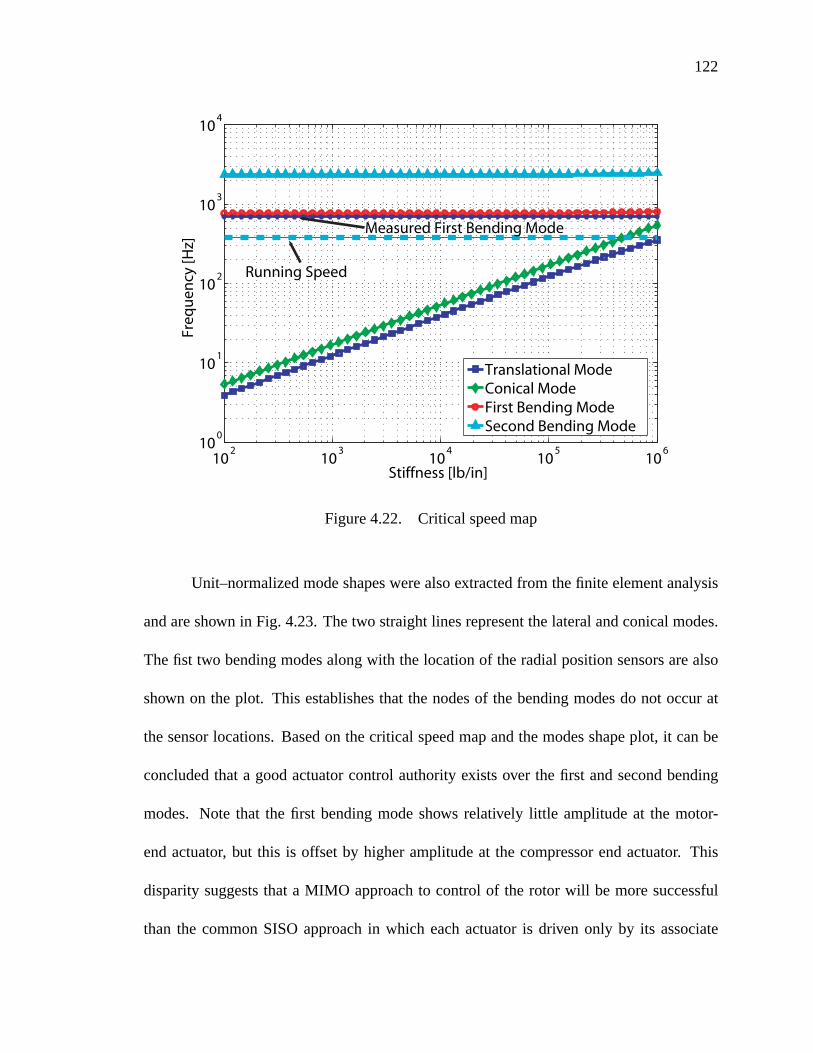
122

102

103

104

105

10610

0

101

102

103

104

Freq

uenc

y [H

z]

Stiffness [lb/in]

Translational ModeConical ModeFirst Bending ModeSecond Bending Mode

Running Speed

Measured First Bending Mode

Figure 4.22. Critical speed map

Unit–normalized mode shapes were also extracted from the finite element analysis

and are shown in Fig. 4.23. The two straight lines represent the lateral and conical modes.

The fist two bending modes along with the location of the radial position sensors are also

shown on the plot. This establishes that the nodes of the bending modes do not occur at

the sensor locations. Based on the critical speed map and the modes shape plot, it can be

concluded that a good actuator control authority exists over the first and second bending

modes. Note that the first bending mode shows relatively little amplitude at the motor-

end actuator, but this is offset by higher amplitude at the compressor end actuator. This

disparity suggests that a MIMO approach to control of the rotor will be more successful

than the common SISO approach in which each actuator is driven only by its associate

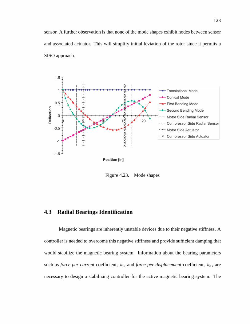
123

sensor. A further observation is that none of the mode shapes exhibit nodes between sensor

and associated actuator. This will simplify initial leviation of the rotor since it permits a

SISO approach.

-1.5

-1

-0.5

0

0.5

1

1.5

0 5 10 15 20 25

Position [in]

Def

lect

ion

Translational Mode

Conical Mode

First Bending Mode

Second Bending Mode

Motor Side Radial Sensor

Compressor Side Radial Sensor

Motor Side Actuator

Compressor Side Actuator

Figure 4.23. Mode shapes

4.3 Radial Bearings Identification

Magnetic bearings are inherently unstable devices due to their negative stiffness. A

controller is needed to overcome this negative stiffness and provide sufficient damping that

would stabilize the magnetic bearing system. Information about the bearing parameters

such as force per current coefficient, ki , and force per displacement coefficient, kx , are

necessary to design a stabilizing controller for the active magnetic bearing system. The

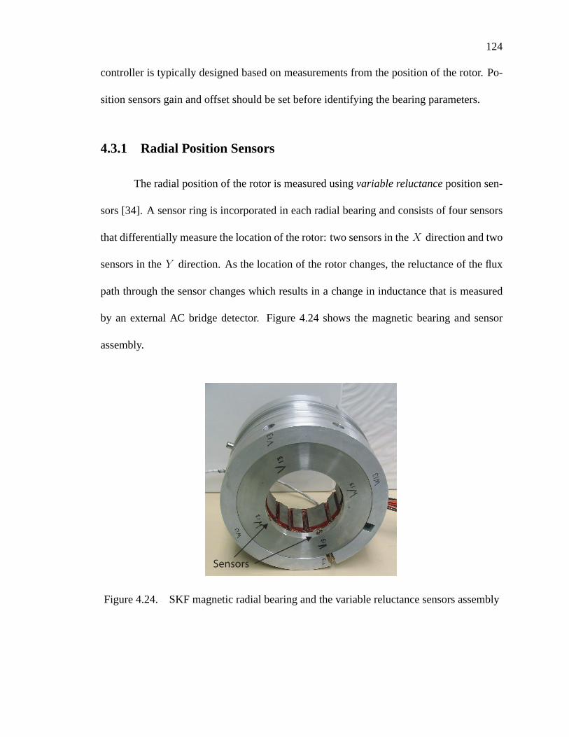
124

controller is typically designed based on measurements from the position of the rotor. Po-

sition sensors gain and offset should be set before identifying the bearing parameters.

4.3.1 Radial Position Sensors

The radial position of the rotor is measured using variable reluctance position sen-

sors [34]. A sensor ring is incorporated in each radial bearing and consists of four sensors

that differentially measure the location of the rotor: two sensors in the X direction and two

sensors in the Y direction. As the location of the rotor changes, the reluctance of the flux

path through the sensor changes which results in a change in inductance that is measured

by an external AC bridge detector. Figure 4.24 shows the magnetic bearing and sensor

assembly.

Sensors

Figure 4.24. SKF magnetic radial bearing and the variable reluctance sensors assembly

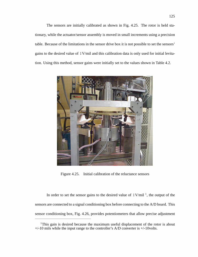
125

The sensors are initially calibrated as shown in Fig. 4.25. The rotor is held sta-

tionary, while the actuator/sensor assembly is moved in small increments using a precision

table. Because of the limitations in the sensor drive box it is not possible to set the sensors’

gains to the desired value of 1V/mil and this calibration data is only used for initial levita-

tion. Using this method, sensor gains were initially set to the values shown in Table 4.2.

Figure 4.25. Initial calibration of the reluctance sensors

In order to set the sensor gains to the desired value of 1V/mil 1, the output of the

sensors are connected to a signal conditioning box before connecting to the A/D board. This

sensor conditioning box, Fig. 4.26, provides potentiometers that allow precise adjustment

1This gain is desired because the maximum useful displacement of the rotor is about+/-10 mils while the input range to the controller’s A/D converter is +/-10volts.

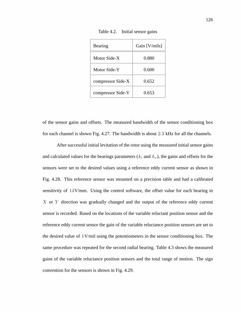
126

Table 4.2. Initial sensor gains

Bearing Gain [V/mils]

Motor Side-X 0.880

Motor Side-Y 0.600

compressor Side-X 0.652

compressor Side-Y 0.653

of the sensor gains and offsets. The measured bandwidth of the sensor conditioning box

for each channel is shown Fig. 4.27. The bandwidth is about 2.3 kHz for all the channels.

After successful initial levitation of the rotor using the measured initial sensor gains

and calculated values for the bearings parameters (ki and kx ), the gains and offsets for the

sensors were set to the desired values using a reference eddy current sensor as shown in

Fig. 4.28. This reference sensor was mounted on a precision table and had a calibrated

sensitivity of 14V/mm. Using the control software, the offset value for each bearing in

X or Y direction was gradually changed and the output of the reference eddy current

sensor is recorded. Based on the locations of the variable reluctant position sensor and the

reference eddy current sensor the gain of the variable reluctance position sensors are set to

the desired value of 1V/mil using the potentiometers in the sensor conditioning box. The

same procedure was repeated for the second radial bearing. Table 4.3 shows the measured

gains of the variable reluctance position sensors and the total range of motion. The sign

convention for the sensors is shown in Fig. 4.29.

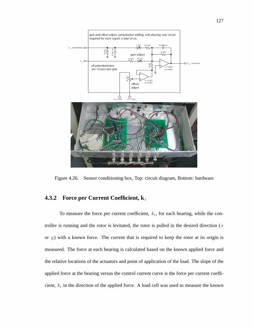
127

V x1

1.0 k Ω

10k Ω

10

k Ω

10 k Ω

+12.1 V DC -12.1 VDC

0.0068 µfV x1 , perturbation

8.2 k Ω

10

kΩ

0.0

01

µf

Vx1

, corrected

gain adjust

offsetadjust

10 k Ω

5 kΩ

gain and offset adjust, perturbation adding, anti-aliasing: one circuitrequired for each signal: a total of six

½ T L 082or s imilar

all potentiometersare 10-turn trim pots

½ T L 082or s imilar

Figure 4.26. Sensor conditioning box, Top: circuit diagram, Bottom: hardware

4.3.2 Force per Current Coefficient, ki

To measure the force per current coefficient, ki , for each bearing, while the con-

troller is running and the rotor is levitated, the rotor is pulled in the desired direction (x

or y ) with a known force. The current that is required to keep the rotor at its origin is

measured. The force at each bearing is calculated based on the known applied force and

the relative locations of the actuators and point of application of the load. The slope of the

applied force at the bearing versus the control current curve is the force per current coeffi-

cient, ki in the direction of the applied force. A load cell was used to measure the known

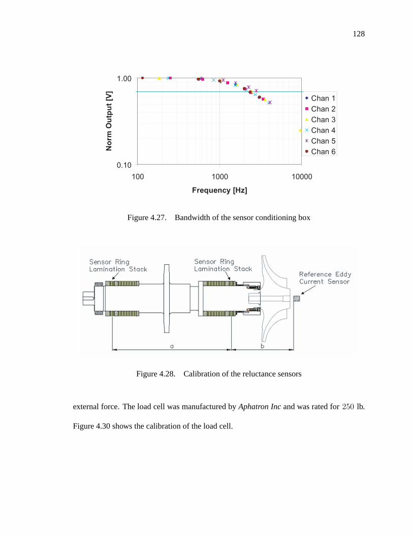
128

0.10

1.00

100 1000 10000

Frequency [Hz]

Nor

m O

utpu

t [V] Chan 1

Chan 2Chan 3Chan 4Chan 5Chan 6

Figure 4.27. Bandwidth of the sensor conditioning box

Figure 4.28. Calibration of the reluctance sensors

external force. The load cell was manufactured by Aphatron Inc and was rated for 250 lb.

Figure 4.30 shows the calibration of the load cell.

129

Table 4.3. Sensor gains and range of motion

Bearing Gain [V/mils] Total clearance [mils]

Motor Side-X 1.0145 13.04

Motor Side-Y 0.9961 14.09

compressor Side-X 1.0085 14.48

compressor Side-Y 0.9718 14.52

Figure 4.29. Sensors sign convention

Motor Side ki

A disturbance force was applied in the direction that ki is being measured using a

pulley and weights system. The resulting force at the bearings was calculated based on the

location of the applied disturbance force and the bearing locations on the rotor. Figure 4.31

shows the free body diagram of the applied disturbance force and the resulting bearing

forces. The forces at the bearing locations were calculated according to (4.1a) and (4.1b).

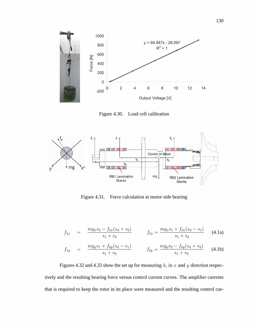
130

y = 69.847x - 28.097R2 = 1

-200

0

200

400

600

800

1000

0 2 4 6 8 10 12 14

Output Voltage [V]

Forc

e [N

]

Figure 4.30. Load cell calibration

Figure 4.31. Force calculation at motor side bearing

f1x =mgxs2 − fdx(sd + s2)

s1 + s2

f2x =mgxs1 + fdx(sd − s1)

s1 + s2

(4.1a)

f1y =mgys1 + fdy(sd − s1)

s1 + s2

f2y =mgys2 − fdy(sd + s2)

s1 + s2

(4.1b)

Figures 4.32 and 4.33 show the set up for measuring ki in x and y direction respec-

tively and the resulting bearing force versus control current curves. The amplifier currents

that is required to keep the rotor in its place were measured and the resulting control cur-

131

rents were calculated. The saturation force for the motor side radial bearing is computed

as 300 lb (1334 N) in each direction. The disturbance force was varied from 0 to 200 lbs.

The experiment was repeated two times. The data exhibited a very linear trend over the

entire range of the available bearing force.

y = 280.36x - 160.39R2 = 0.9996

y = 284.58x - 159.46R2 = 0.9995

-1400

-1200

-1000

-800

-600

-400

-200

0

200

-4.0 -3.0 -2.0 -1.0 0.0 1.0 2.0

Control Current ix [A]

F x [

N]

1st

2nd

Linear (1st)

Linear (2nd)

Figure 4.32. Measurement of ki in x direction for the motor side radial bearing

y = 298.61x - 106.89R2 = 0.9992

y = 301.04x - 105.98R2 = 0.9987

-1400

-1200

-1000

-800

-600

-400

-200

0

200

-4.0 -3.0 -2.0 -1.0 0.0 1.0

Control Current iy [A]

Fy [

N] 1st

2ndLinear (1st)Linear (2nd)

Figure 4.33. Measurement of ki in y direction for the motor side radial bearing

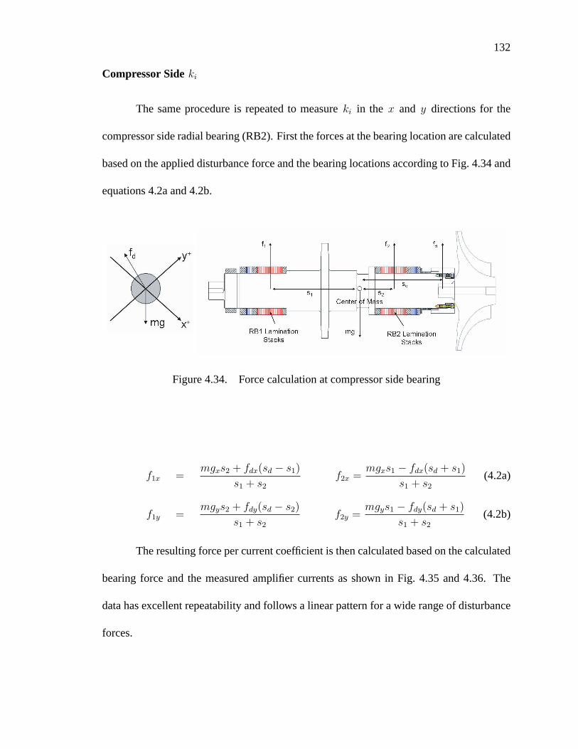
132

Compressor Side ki

The same procedure is repeated to measure ki in the x and y directions for the

compressor side radial bearing (RB2). First the forces at the bearing location are calculated

based on the applied disturbance force and the bearing locations according to Fig. 4.34 and

equations 4.2a and 4.2b.

Figure 4.34. Force calculation at compressor side bearing

f1x =mgxs2 + fdx(sd − s1)

s1 + s2

f2x =mgxs1 − fdx(sd + s1)

s1 + s2

(4.2a)

f1y =mgys2 + fdy(sd − s2)

s1 + s2

f2y =mgys1 − fdy(sd + s1)

s1 + s2

(4.2b)

The resulting force per current coefficient is then calculated based on the calculated

bearing force and the measured amplifier currents as shown in Fig. 4.35 and 4.36. The

data has excellent repeatability and follows a linear pattern for a wide range of disturbance

forces.

133

y = 243.81x + 8.5767R2 = 0.9996

y = 246.42x + 10.634R2 = 0.9996

-1200

-1000

-800

-600

-400

-200

0

200

400

-5.00 -4.00 -3.00 -2.00 -1.00 0.00 1.00

Control Current ix [A]

Fx [N

] 2nd1stLinear (2nd)Linear (1st)

Figure 4.35. Measurement of ki in x direction for the compressor side radial bearing

y = 255.59x - 146.39R2 = 0.9995

y = 255.54x - 148.76R2 = 0.9997

-1200

-1000

-800

-600

-400

-200

0

200

400

-4.0 -3.0 -2.0 -1.0 0.0 1.0 2.0

Control Current iy [A]

Fy [N

] 1st2ndLinear (1st)Linear (2nd)

Figure 4.36. Measurement of ki in y direction for the compressor side radial bearing

4.3.3 Open-Loop Stiffness, kx

In order to measure the open-loop stiffness (force per displacement coefficient), kx ,

the rotor is moved parallel to the direction that kx is being measured using the control pro-

gram. The required current that is needed to keep the rotor at the new location is measured

and the resulting control current is calculated. The total instantaneous force acting on the

134

rotor at each offset location is calculated according to (4.3a) and (4.3b):

F1 = x1kx + i1ki (4.3a)

F2 = x2kx + i2ki (4.3b)

Using the current measurement and knowing the force per current coefficient, ki ,

from previous measurements, the force per current coefficient, kx , is calculated according

to (4.4):

F1 = F2 → kx =(i1 − i2)ki

x1 − x2

(4.4)

Figures 4.37 and 4.38 show how the force generated by the control current, iki ,

varies as the rotor moves to different offset locations in x and y directions respectively for

both the motor side radial bearing and the compressor side radial bearing. The experiment

is repeated two times in each direction and the resulting force follows a linear trend with

an excellent repeatability. This shows that the data can confidently be used to calculate the

force per displacement coefficient, kx . The resulting kx values for both radial bearings at

different bias currents are summarized in table 4.5.

4.4 Thrust Bearing Identification

The same identification technique is used to identify the ki and kx for the thrust

bearing.

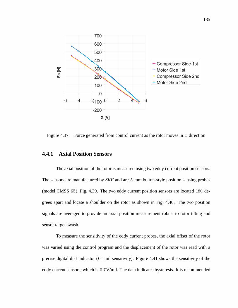
135

-200

-100

0

100

200

300

400

500

600

700

-6 -4 -2 0 2 4 6

X [V]

Fc [N

] Compressor Side 1stMotor Side 1stCompressor Side 2ndMotor Side 2nd

Figure 4.37. Force generated from control current as the rotor moves in x direction

4.4.1 Axial Position Sensors

The axial position of the rotor is measured using two eddy current position sensors.

The sensors are manufactured by SKF and are 5 mm button-style position sensing probes

(model CMSS 65), Fig. 4.39. The two eddy current position sensors are located 180 de-

grees apart and locate a shoulder on the rotor as shown in Fig. 4.40. The two position

signals are averaged to provide an axial position measurement robust to rotor tilting and

sensor target swash.

To measure the sensitivity of the eddy current probes, the axial offset of the rotor

was varied using the control program and the displacement of the rotor was read with a

precise digital dial indicator (0.1mil sensitivity). Figure 4.41 shows the sensitivity of the

eddy current sensors, which is 0.7V/mil. The data indicates hysteresis. It is recommended

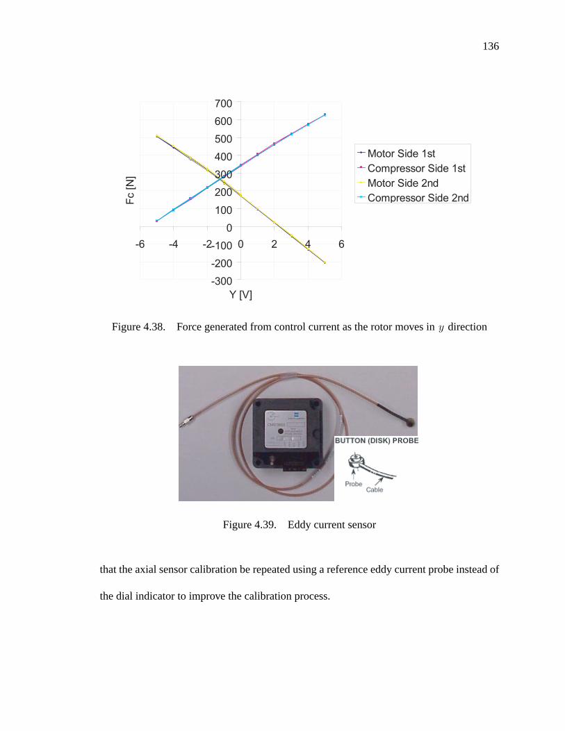
136

-300-200-100

0100

200300400500600700

-6 -4 -2 0 2 4 6

Y [V]

Fc [N

]

Motor Side 1stCompressor Side 1stMotor Side 2ndCompressor Side 2nd

Figure 4.38. Force generated from control current as the rotor moves in y direction

Figure 4.39. Eddy current sensor

that the axial sensor calibration be repeated using a reference eddy current probe instead of

the dial indicator to improve the calibration process.

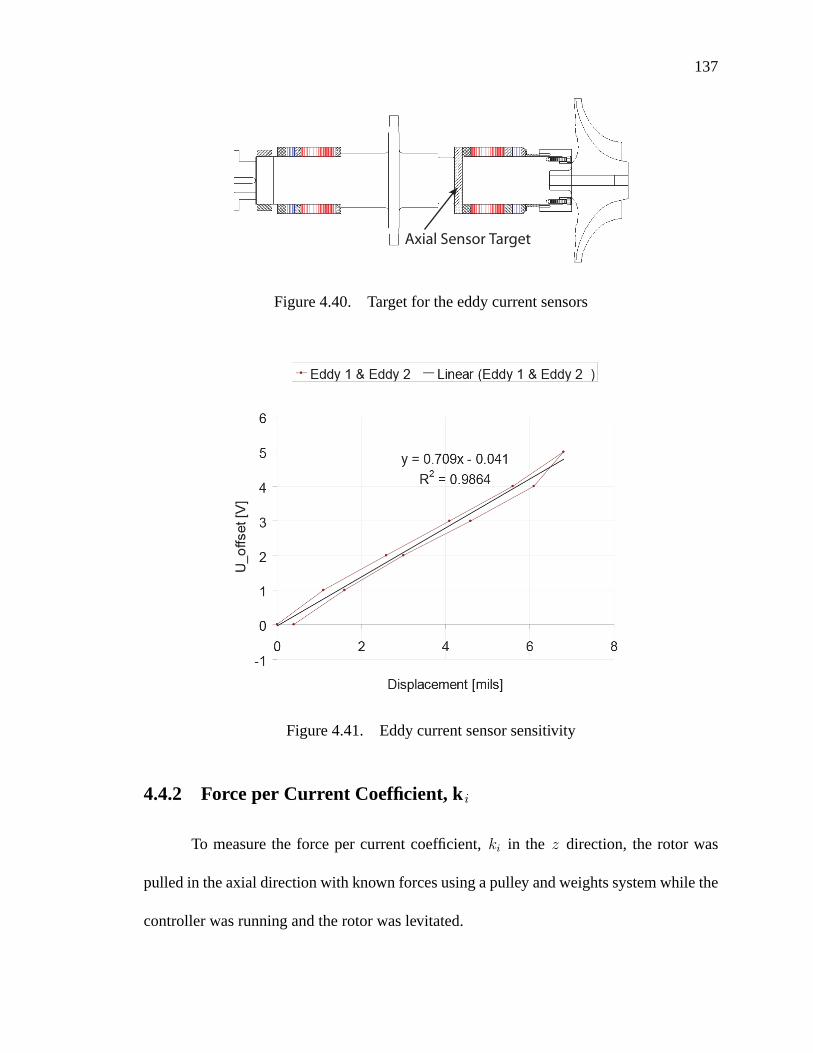
137

Axial Sensor Target

Figure 4.40. Target for the eddy current sensors

Figure 4.41. Eddy current sensor sensitivity

4.4.2 Force per Current Coefficient, ki

To measure the force per current coefficient, ki in the z direction, the rotor was

pulled in the axial direction with known forces using a pulley and weights system while the

controller was running and the rotor was levitated.

138

The amplifier current that is required to keep the rotor axially in its place is mea-

sured and the resulting control current versus the bearing force is plotted in Fig. 4.42. The

compressor manufacturer has predicted an impeller load of 3300 N at the design operating

point. To accommodate for the unpredicted forces encountered in the surge regime and the

dynamic capacity derating due to eddy current effects at high frequencies, the thrust bear-

ing is designed with a high safety factor of 2, to withstand 6600 N with a bias current of

7 A. Because of the maximum load capacity limitation of the available load cell (250 lb),

it is not possible to do measurements for the entire range of thrust bearing load capacity.

Therefore, the experiments are done up to the point that is possible to obtain reliable mea-

surement using the current load cell. However, since this data shows a very repeatable and

linear curve, it is assumed that the trend is valid for the rest of bearing load capacity range.

y = 1158.4x - 353.51R2 = 0.9974

y = 1137.5x - 340.88R2 = 0.9993

0

100

200

300

400

500

600

700

800

900

1000

0.0 0.5 1.0 1.5

Control Current iz [A]

Fz [N

] 1st2ndLinear (1st)Linear (2nd)

Figure 4.42. Measurement of ki for the thrust bearing

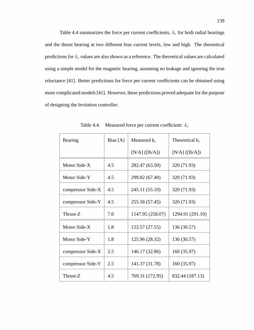
139

Table 4.4 summarizes the force per current coefficients, ki for both radial bearings

and the thrust bearing at two different bias current levels, low and high. The theoretical

predictions for ki values are also shown as a reference. The theoretical values are calculated

using a simple model for the magnetic bearing, assuming no leakage and ignoring the iron

reluctance [41]. Better predictions for force per current coefficients can be obtained using

more complicated models [41]. However, these predictions proved adequate for the purpose

of designing the levitation controller.

Table 4.4. Measured force per current coefficient: ki

Bearing Bias [A] Measured ki Theoretical ki

[N/A] ([lb/A]) [N/A] ([lb/A])

Motor Side-X 4.5 282.47 (63.50) 320 (71.93)

Motor Side-Y 4.5 299.82 (67.40) 320 (71.93)

compressor Side-X 4.5 245.11 (55.10) 320 (71.93)

compressor Side-Y 4.5 255.56 (57.45) 320 (71.93)

Thrust-Z 7.0 1147.95 (258.07) 1294.91 (291.10)

Motor Side-X 1.8 122.57 (27.55) 136 (30.57)

Motor Side-Y 1.8 125.96 (28.32) 136 (30.57)

compressor Side-X 2.5 146.17 (32.86) 160 (35.97)

compressor Side-Y 2.5 141.37 (31.78) 160 (35.97)

Thrust-Z 4.5 769.31 (172.95) 832.44 (187.13)

140

4.4.3 Open-Loop Stiffness, kx

The same procedure (as in the case of radial bearings) was repeated to measure the

open-loop stiffness (force per displacement coefficient), kx , for the thrust bearing. The

rotor was moved to different offset locations using the control program. The required

current to keep the rotor at the new location was measured and the resulting control current

was calculated. Using the current measurement and the already known force per current

coefficient, ki , from previous measurements, the force per current coefficient, kx , was

calculated according to (4.4).

Figure 4.43 shows how the force generated by the control current, iki , varies as the

rotor moves to different offset locations in axial, z , direction. The experiment was repeated

two times. The resulting force again follows a linear trend which shows that the data can

confidently be used to calculate the force per displacement coefficient, kx .

-1500

-1000

-500

0

500

1000

1500

2000

2500

-8 -6 -4 -2 0 2 4 6 8

Z [V]

Fc [N

] 1st2nd

Figure 4.43. Measurement of kx for the thrust bearing

141

Table 4.5 summarizes the force per displacement coefficients, kx for both radial

bearings and the thrust bearing at two different bias current levels, low and high along with

their theoretical predictions.

Table 4.5. Measured force per displacement factor: kx

Bearing Bias[A] Measured Theoretical

kx[N/m]([lb/inch]) kx[N/m]([lb/inch])

Motor Side-X 4.5 2.6585e6 (15180) 3.08e6 (17587)

Motor Side-Y 4.5 2.7812e6 (15881) 3.08e6 (17587)

compressor Side-X 4.5 2.2305e6 (12736) 3.08e6 (17587)

compressor Side-Y 4.5 2.2780e6 (13007 3.08e6 (17587)

Thrust-Z 7.0 6.8228e6 (38959) 7.68e6 (43854)

Motor Side-X 1.8 5.0066e5 (2858) 4.92e5 (2809)

Motor Side-Y 1.8 5.0215e5 (2867) 4.92e5 (2809)

compressor Side-X 2.5 9.7195e5 (5550) 9.50e5 (5424)

compressor Side-Y 2.5 9.2994e5 (5310) 9.50e5 (5424)

Thrust-Z 4.5 3.0693e6 (17526) 3.67e6 (20956)

Knowing all the bearing parameters, the controller was redesigned with the identi-

fied values for ki, kx and the sensor gains.

142

4.5 Amplifier Identification

The power amplifiers that are used to drive the magnetic bearings are DC servo

switching amplifiers manufactured by Copley Controls-(Model 423). These 25 kHz switch-

ing amplifiers can provide a maximum continuous current of 15A at 170V and a maximum

peak current of 30A at 170V. Table 4.6 summarizes the properties of the power amplifiers.

More information about the amplifiers are provided in Appendix C. The configuration and

matching of the amplifiers and sensors is summarized in Table 4.7.

Table 4.6. Power amplifiers specifications

Switching Frequency 25[kHz]

Supply Voltage 141[VDC]

Continuous Current 15[A]

Peak Current 30[A]

Gain 1.5[A/V] (see Appendix C)

Amplifier Offset 0.002[A]

Current Monitor 4.87-4.94[A/V] (see Appendix C)

Inductance (Amplifiers 1-8) 15-25[mH]

Inductance (Amplifiers 9-10) 48-52[mH]

The amplifier transfer function was measured using a sine sweep with a magnitude

of 1 A. Figure 4.44 shows the measured transfer function from the sine sweep test and a

143

Table 4.7. Amplifier and sensor configuration

Direction Amplifier Sensor [Revolve] (Sensor Conditioning)

Motor Side Radial Bearing (RB1)

X1 #4 [-V24] (+Channel 3)

X2 #2 [+V24] (-Channel 3)

Y1 #3 [+W24] (+Channel 4)

Y2 #1 [-W24] (-Channel 4)

Compressor Side Radial Bearing (RB2)

X1 #8 [-W13] (+Channel 2)

X2 #6 [+W13] (-Channel 2)

Y1 #7 [-V13] (-Channel 1)

Y2 #5 [+V13] (+Channel 1)

Thrust Bearing

Z1 #10 [less negative] (-Channel 5/6)

Z2 #9 [more negative] (+Channel 5/6)

model that matches the data very well. The model is a first order model with a bandwidth

of 620 Hz and a time delay of 0.1444 msec.

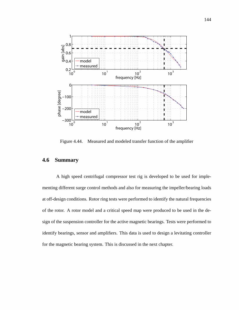
144

100

101

102

1030.2

0.4

0.6

0.8

1

gain

[abs

]

frequency [Hz]

modelmeasured

100

101

102

103−300

−200

−100

0

phas

e [d

egre

e]

frequency [Hz]

modelmeasured

Figure 4.44. Measured and modeled transfer function of the amplifier

4.6 Summary

A high speed centrifugal compressor test rig is developed to be used for imple-

menting different surge control methods and also for measuring the impeller/bearing loads

at off-design conditions. Rotor ring tests were performed to identify the natural frequencies

of the rotor. A rotor model and a critical speed map were produced to be used in the de-

sign of the suspension controller for the active magnetic bearings. Tests were performed to

identify bearings, sensor and amplifiers. This data is used to design a levitating controller

for the magnetic bearing system. This is discussed in the next chapter.

145

CHAPTER 5

MAGNETIC LEVITATION

5.1 Magnetic Bearing Overview

The principle of operation of an active magnetic bearing system may be explained

using Fig. 5.1. The primary goal is to keep the rotor in a desired position. A non-contacting

sensor measures the position of the rotor and provides this displacement information to the

controller. The controller uses a control law to compute the required current to keep the

error between the desired and actual position small. The power amplifier applies a voltage

trajectory to the coil which attempts to meet this target current to keep the rotor in the

desired location. The specific parameters of the control law govern the resulting stiffness

and damping of the suspension [41].

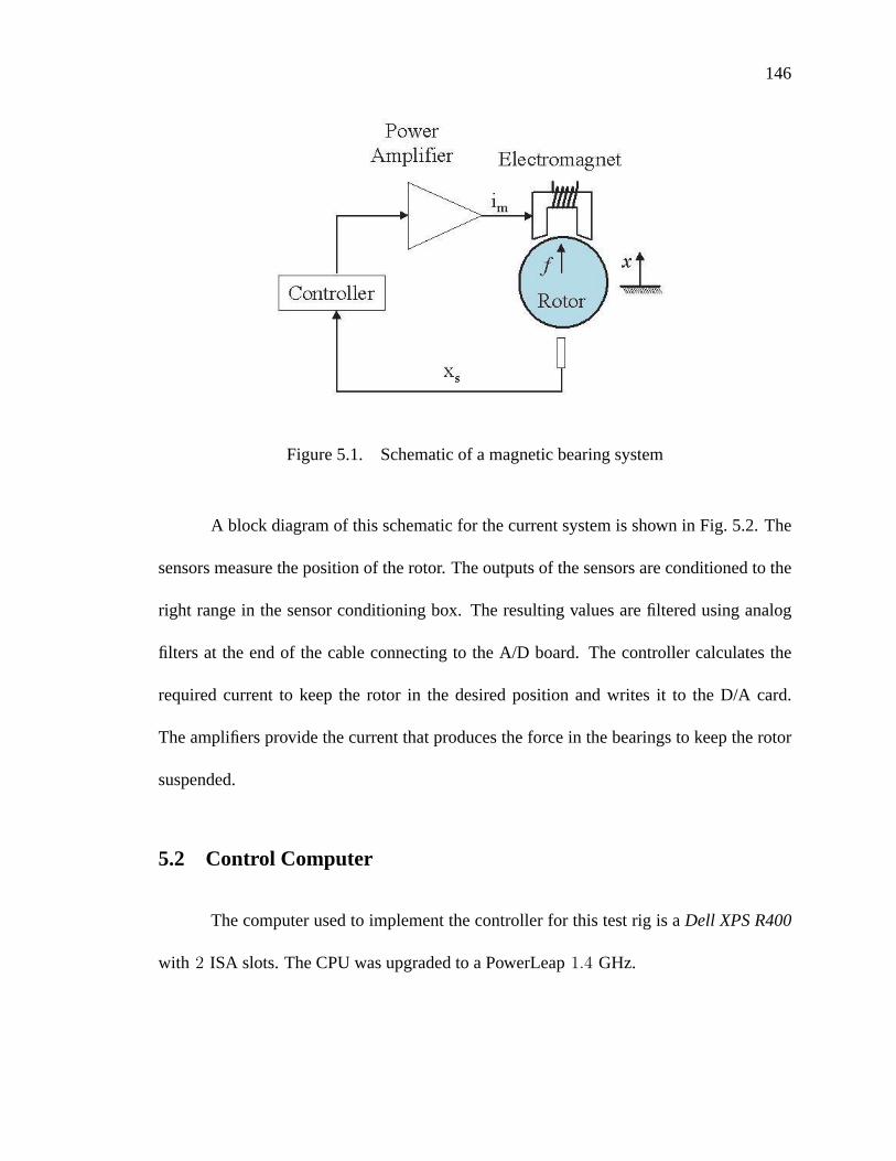
146

Figure 5.1. Schematic of a magnetic bearing system

A block diagram of this schematic for the current system is shown in Fig. 5.2. The

sensors measure the position of the rotor. The outputs of the sensors are conditioned to the

right range in the sensor conditioning box. The resulting values are filtered using analog

filters at the end of the cable connecting to the A/D board. The controller calculates the

required current to keep the rotor in the desired position and writes it to the D/A card.

The amplifiers provide the current that produces the force in the bearings to keep the rotor

suspended.

5.2 Control Computer

The computer used to implement the controller for this test rig is a Dell XPS R400

with 2 ISA slots. The CPU was upgraded to a PowerLeap 1.4 GHz.

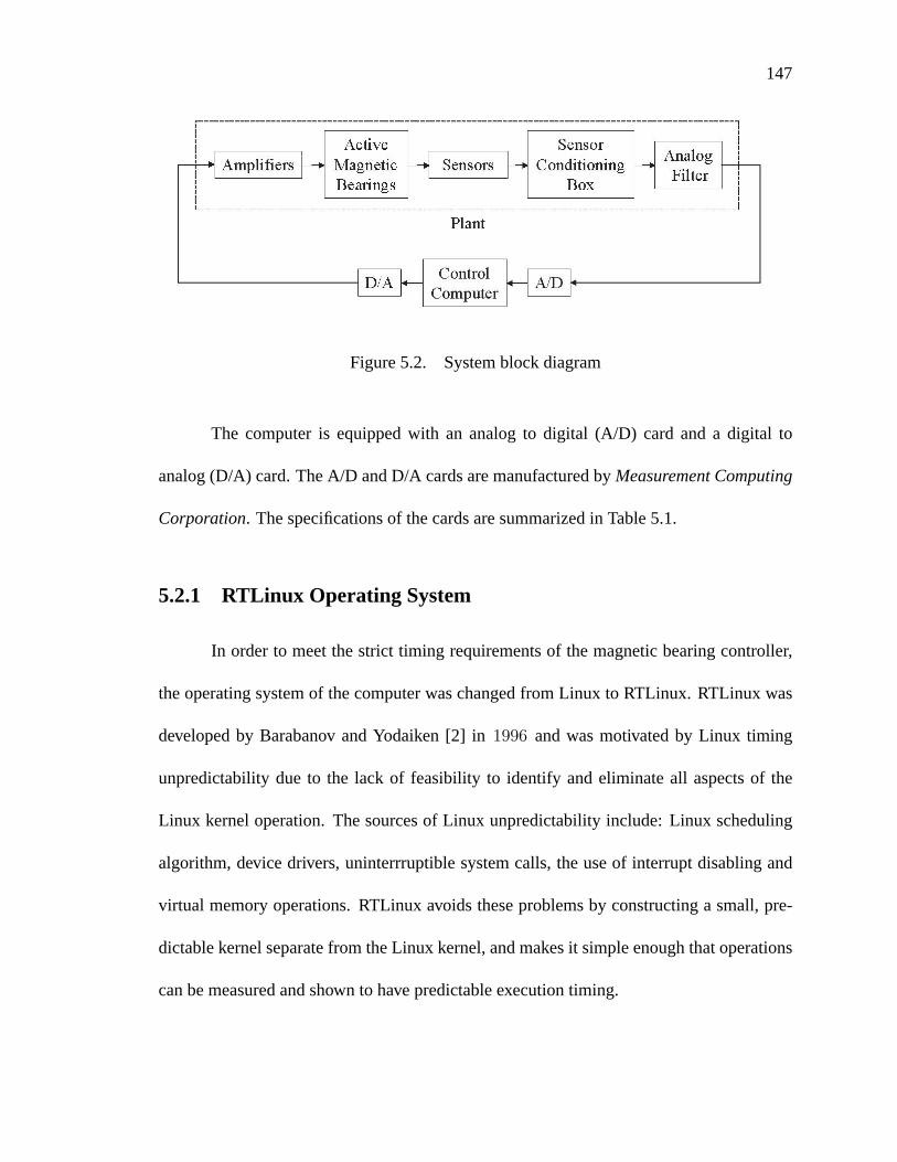
147

Figure 5.2. System block diagram

The computer is equipped with an analog to digital (A/D) card and a digital to

analog (D/A) card. The A/D and D/A cards are manufactured by Measurement Computing

Corporation. The specifications of the cards are summarized in Table 5.1.

5.2.1 RTLinux Operating System

In order to meet the strict timing requirements of the magnetic bearing controller,

the operating system of the computer was changed from Linux to RTLinux. RTLinux was

developed by Barabanov and Yodaiken [2] in 1996 and was motivated by Linux timing

unpredictability due to the lack of feasibility to identify and eliminate all aspects of the

Linux kernel operation. The sources of Linux unpredictability include: Linux scheduling

algorithm, device drivers, uninterrruptible system calls, the use of interrupt disabling and

virtual memory operations. RTLinux avoids these problems by constructing a small, pre-

dictable kernel separate from the Linux kernel, and makes it simple enough that operations

can be measured and shown to have predictable execution timing.

148

Table 5.1. Data acquisition cards specifications

Analog to Digital Card Digital to Analog Card

Model: CIO-DAS1402/16 Model: CIO-DAC16

Base Channel: 0x300 Base Address: 0x320

16-bit (1 in 65536) 12 bits (1 in 4095)

Number of Channels: 8 differential inputs Number of Channels: 16 single-ended outputs

Output Range: ±10V Output Range: ±10V

Resolution: 0.30mV Resolution: 4.80mV

Burstmode: 13.3µ sec Settling time: 70µ sec

A/D conversion time: 10µ sec Slew Rate: 0.3V/µ sec

Throughput: 100kHz

Figure 5.3 shows the basic Linux kernel without hard realtime support. The Linux

kernel separates the hardware from user-level tasks. The kernel has the ability to suspend

any user-level task, once that task has outrun the slice of time allotted to it by the CPU. In

running the controller for the magnetic bearings, the standard Linux kernel at some instants

preempts the task and gives the CPU to a task which is less critical (e.g. one that boots

up Netscape). Consequently, the magnetic bearing controller does not meet strict timing

requirements and looses levitation. Thus, in trying to be fair to all tasks, the standard Linux

kernel prevents critical events from real-time execution.

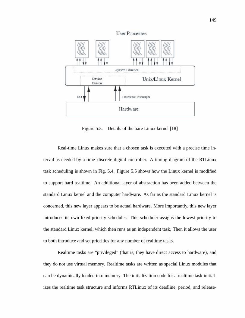
149

Figure 5.3. Details of the bare Linux kernel [18]

Real-time Linux makes sure that a chosen task is executed with a precise time in-

terval as needed by a time–discrete digital controller. A timing diagram of the RTLinux

task scheduling is shown in Fig. 5.4. Figure 5.5 shows how the Linux kernel is modified

to support hard realtime. An additional layer of abstraction has been added between the

standard Linux kernel and the computer hardware. As far as the standard Linux kernel is

concerned, this new layer appears to be actual hardware. More importantly, this new layer

introduces its own fixed-priority scheduler. This scheduler assigns the lowest priority to

the standard Linux kernel, which then runs as an independent task. Then it allows the user

to both introduce and set priorities for any number of realtime tasks.

Realtime tasks are “privileged” (that is, they have direct access to hardware), and

they do not use virtual memory. Realtime tasks are written as special Linux modules that

can be dynamically loaded into memory. The initialization code for a realtime task initial-

izes the realtime task structure and informs RTLinux of its deadline, period, and release-

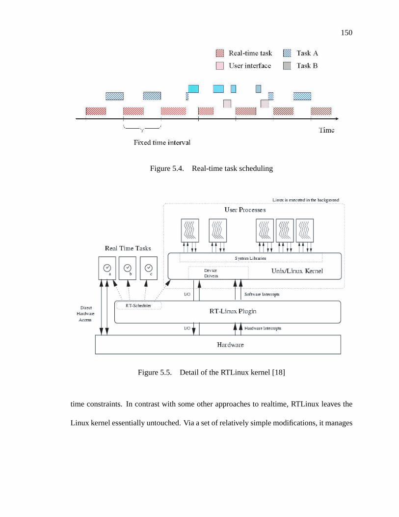
150

Figure 5.4. Real-time task scheduling

Figure 5.5. Detail of the RTLinux kernel [18]

time constraints. In contrast with some other approaches to realtime, RTLinux leaves the

Linux kernel essentially untouched. Via a set of relatively simple modifications, it manages

151

to convert the existing Linux kernel into a hard realtime environment without hindering fu-

ture Linux development1.

5.2.2 Control Software

The control software is programmed in C. Instructions on how to operate the con-

trol program are provided in Appendix D. Figure 5.6 shows the structure of the control

software. First the user should load a controller. The control matrices are generated in

Matlab. The development of the control matrices is explained in the next section. The user

can modify the control settings such as the offset of the rotor and perturbation level and

frequencies for each bearing and in X or Y direction. The realtime task first reads the

sensor signals from the A/D convertor and propagates the states. The required current to

keep the rotor at the preset reference position is calculated and is written to the D/A cards.

The position of the rotor and the commanded bearing currents are recorded in a ring buffer

and can be accessed by a non–realtime user interface or written to the hard drive.

5.3 Thrust Bearing Controller

In order to design a levitating controller for the thrust direction, one should first

obtain a good model of the thrust bearing itself. The next section discusses the modeling

of the magnetic thrust bearing.

1For a more detailed discussion, see [18].

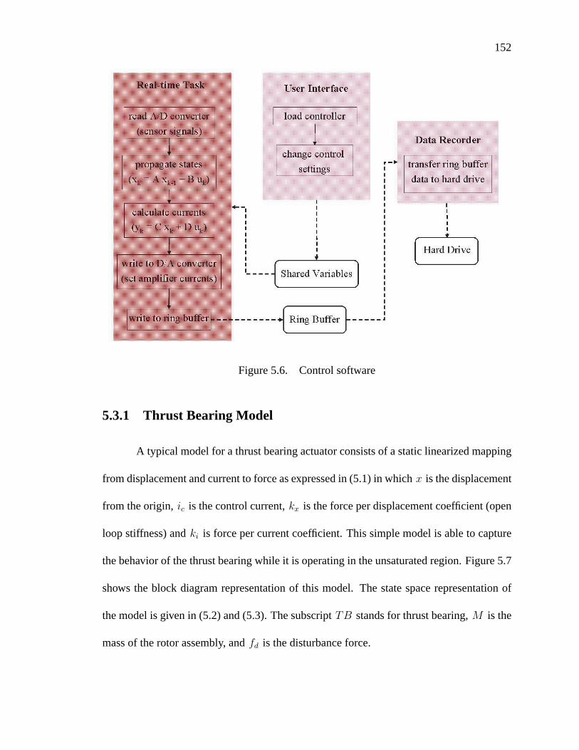
152

Figure 5.6. Control software

5.3.1 Thrust Bearing Model

A typical model for a thrust bearing actuator consists of a static linearized mapping

from displacement and current to force as expressed in (5.1) in which x is the displacement

from the origin, ic is the control current, kx is the force per displacement coefficient (open

loop stiffness) and ki is force per current coefficient. This simple model is able to capture

the behavior of the thrust bearing while it is operating in the unsaturated region. Figure 5.7

shows the block diagram representation of this model. The state space representation of

the model is given in (5.2) and (5.3). The subscript TB stands for thrust bearing, M is the

mass of the rotor assembly, and fd is the disturbance force.

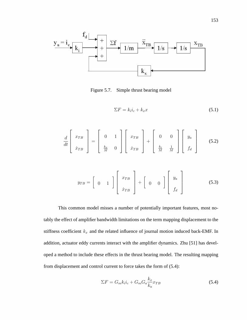
153

Figure 5.7. Simple thrust bearing model

ΣF = kiic + kxx (5.1)

d

dt

xTB

xTB

=

0 1

kx

M0

xTB

xTB

+

0 0

ki

M1M

ya

fd

(5.2)

yTB =

[0 1

] xTB

xTB

+

[0 0

] ya

fd

(5.3)

This common model misses a number of potentially important features, most no-

tably the effect of amplifier bandwidth limitations on the term mapping displacement to the

stiffness coefficient kx and the related influence of journal motion induced back-EMF. In

addition, actuator eddy currents interact with the amplifier dynamics. Zhu [51] has devel-

oped a method to include these effects in the thrust bearing model. The resulting mapping

from displacement and control current to force takes the form of (5.4):

ΣF = Gmkiic +GmGakx

ka

xTB (5.4)

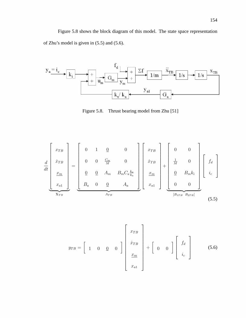
154

Figure 5.8 shows the block diagram of this model. The state space representation

of Zhu’s model is given in (5.5) and (5.6).

Figure 5.8. Thrust bearing model from Zhu [51]

d

dt

xTB

xTB

xm

xa1

︸︷︷︸XTB

=

0 1 0 0

0 0 Cm

M0

0 0 Am BmCakx

ka

Ba 0 0 Aa

︸︷︷︸ATB

xTB

xTB

xm

xa1

+

0 0

1M

0

0 Bmki

0 0

︸︷︷︸[B1TB B2TB ]

fd

ic

(5.5)

yTB =

[1 0 0 0

]

xTB

xTB

xm

xa1

+

[0 0

] fd

ic

(5.6)

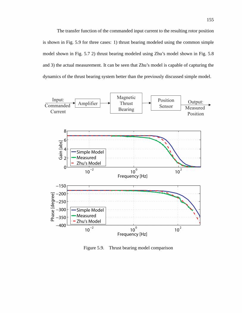
155

The transfer function of the commanded input current to the resulting rotor position

is shown in Fig. 5.9 for three cases: 1) thrust bearing modeled using the common simple

model shown in Fig. 5.7 2) thrust bearing modeled using Zhu’s model shown in Fig. 5.8

and 3) the actual measurement. It can be seen that Zhu’s model is capable of capturing the

dynamics of the thrust bearing system better than the previously discussed simple model.

10−2

100

1020

2

4

6

8

Gai

n [a

bs]

Frequency [Hz]

10−2

100

102−400

−350

−300

−250

−200

−150

Phas

e [d

egre

e]

Frequency [Hz]

Simple ModelMeasuredZhu‘s Model

Simple ModelMeasuredZhu‘s Model

MagneticThrust

Bearing

PositionSensorAmplifier

Input:Commanded

Current

Output:Measured Position

Figure 5.9. Thrust bearing model comparison

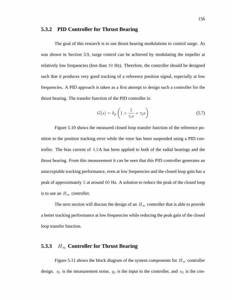
156

5.3.2 PID Controller for Thrust Bearing

The goal of this research is to use thrust bearing modulations to control surge. As

was shown in Section 3.9, surge control can be achieved by modulating the impeller at

relatively low frequencies (less than 10 Hz). Therefore, the controller should be designed

such that it produces very good tracking of a reference position signal, especially at low

frequencies. A PID approach is taken as a first attempt to design such a controller for the

thrust bearing. The transfer function of the PID controller is:

G(s) = kp

(1 +

1

τis+ τds

)(5.7)

Figure 5.10 shows the measured closed loop transfer function of the reference po-

sition to the position tracking error while the rotor has been suspended using a PID con-

troller. The bias current of 4.5A has been applied to both of the radial bearings and the

thrust bearing. From this measurement it can be seen that this PID controller generates an

unacceptable tracking performance, even at low frequencies and the closed loop gain has a

peak of approximately 5 at around 60 Hz. A solution to reduce the peak of the closed loop

is to use an H∞ controller.

The next section will discuss the design of an H∞ controller that is able to provide

a better tracking performance at low frequencies while reducing the peak gain of the closed

loop transfer function.

5.3.3 H∞ Controller for Thrust Bearing

Figure 5.11 shows the block diagram of the system components for H∞ controller

design. η1 is the measurement noise, y2 is the input to the controller, and u2 is the con-

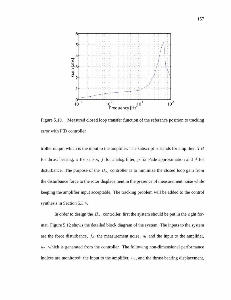
157

10−1

100

101

1020

1

2

3

4

5

6

Gai

n [a

bs]

Frequency [Hz]

Figure 5.10. Measured closed loop transfer function of the reference position to tracking

error with PID controller

troller output which is the input to the amplifier. The subscript a stands for amplifier, TB

for thrust bearing, s for sensor, f for analog filter, p for Pade approximation and d for

disturbance. The purpose of the H∞ controller is to minimize the closed loop gain from

the disturbance force to the rotor displacement in the presence of measurement noise while

keeping the amplifier input acceptable. The tracking problem will be added to the control

synthesis in Section 5.3.4.

In order to design the H∞ controller, first the system should be put in the right for-

mat. Figure 5.12 shows the detailed block diagram of the system. The inputs to the system

are the force disturbance, fd , the measurement noise, η1 and the input to the amplifier,

u2 , which is generated from the controller. The following non-dimensional performance

indices are monitored: the input to the amplifier, u2 , and the thrust bearing displacement,

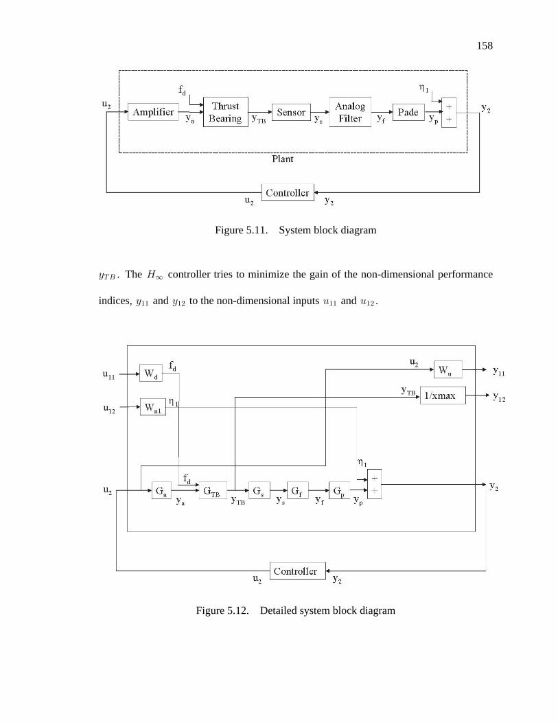
158

Figure 5.11. System block diagram

yTB . The H∞ controller tries to minimize the gain of the non-dimensional performance

indices, y11 and y12 to the non-dimensional inputs u11 and u12 .

Figure 5.12. Detailed system block diagram

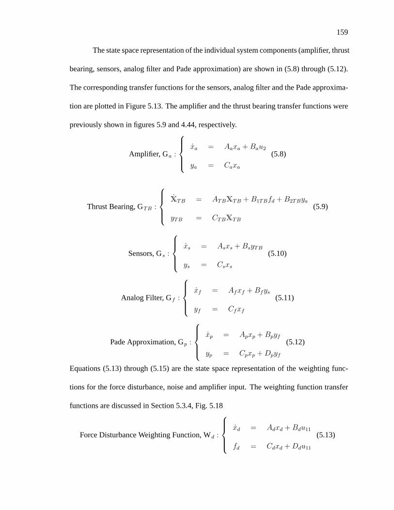
159

The state space representation of the individual system components (amplifier, thrust

bearing, sensors, analog filter and Pade approximation) are shown in (5.8) through (5.12).

The corresponding transfer functions for the sensors, analog filter and the Pade approxima-

tion are plotted in Figure 5.13. The amplifier and the thrust bearing transfer functions were

previously shown in figures 5.9 and 4.44, respectively.

Amplifier, Ga :

xa = Aaxa +Bau2

ya = Caxa

(5.8)

Thrust Bearing, GTB :

XTB = ATBXTB +B1TBfd +B2TBya

yTB = CTBXTB

(5.9)

Sensors, Gs :

xs = Asxs +BsyTB

ys = Csxs

(5.10)

Analog Filter, Gf :

xf = Afxf +Bfys

yf = Cfxf

(5.11)

Pade Approximation, Gp :

xp = Apxp +Bpyf

yp = Cpxp +Dpyf

(5.12)

Equations (5.13) through (5.15) are the state space representation of the weighting func-

tions for the force disturbance, noise and amplifier input. The weighting function transfer

functions are discussed in Section 5.3.4, Fig. 5.18

Force Disturbance Weighting Function, Wd :

xd = Adxd +Bdu11

fd = Cdxd +Ddu11

(5.13)

160

0

1

2

3x 10

4

Mag

nitu

de (a

bs)

102

103

104

105

−90

−45

0Ph

ase

(deg

)

Gs

Frequency (Hz)

0

0.5

1

Mag

nitu

de (a

bs)

102

103

104

105

−90

−45

0

Phas

e (d

eg)

Gf

Frequency (Hz)

0

1

2

Mag

nitu

de (a

bs)

101

102

103

104

105

180

270

360

Phas

e (d

eg)

Gp

Frequency (Hz)

Figure 5.13. Bode plots of the sensors(Gs ), analog filter(Gf ), and Pade

approximation(Gp ) transfer functions

Measurement Noise Weighting Function, Wn1 :

xn1 = An1xn1 +Bn1u12

η1 = Cn1xn1 +Dn1u12

(5.14)

Amplifier Input Weighting Function, Wu :

xu = Auxu +Buu2

y11 = Cuxu +Duu2

(5.15)

This results in a system of 15 states. The system matrices are expressed in (5.16) and

(5.17).

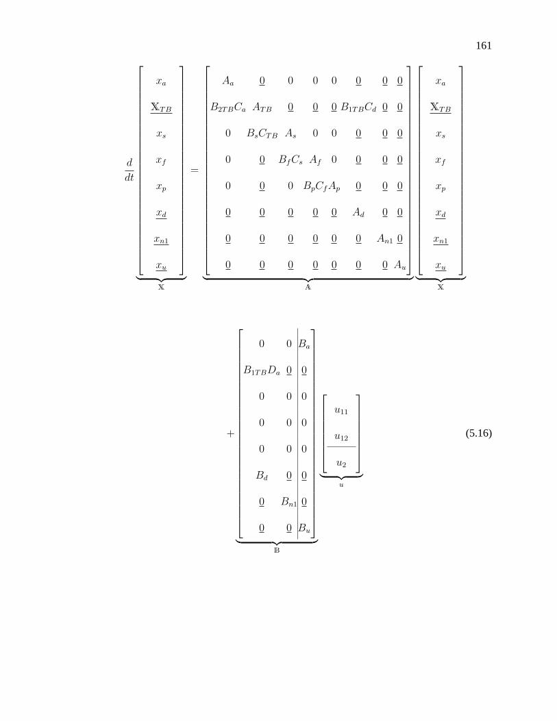
161

d

dt

xa

XTB

xs

xf

xp

xd

xn1

xu

︸︷︷︸X

=

Aa 0 0 0 0 0 0 0

B2TBCa ATB 0 0 0 B1TBCd 0 0

0 BsCTB As 0 0 0 0 0

0 0 BfCs Af 0 0 0 0

0 0 0 BpCfAp 0 0 0

0 0 0 0 0 Ad 0 0

0 0 0 0 0 0 An1 0

0 0 0 0 0 0 0 Au

︸︷︷︸A

xa

XTB

xs

xf

xp

xd

xn1

xu

︸︷︷︸X

+

0 0 Ba

B1TBDa 0 0

0 0 0

0 0 0

0 0 0

Bd 0 0

0 Bn1 0

0 0 Bu

︸︷︷︸B

u11

u12

u2

︸︷︷︸u

(5.16)

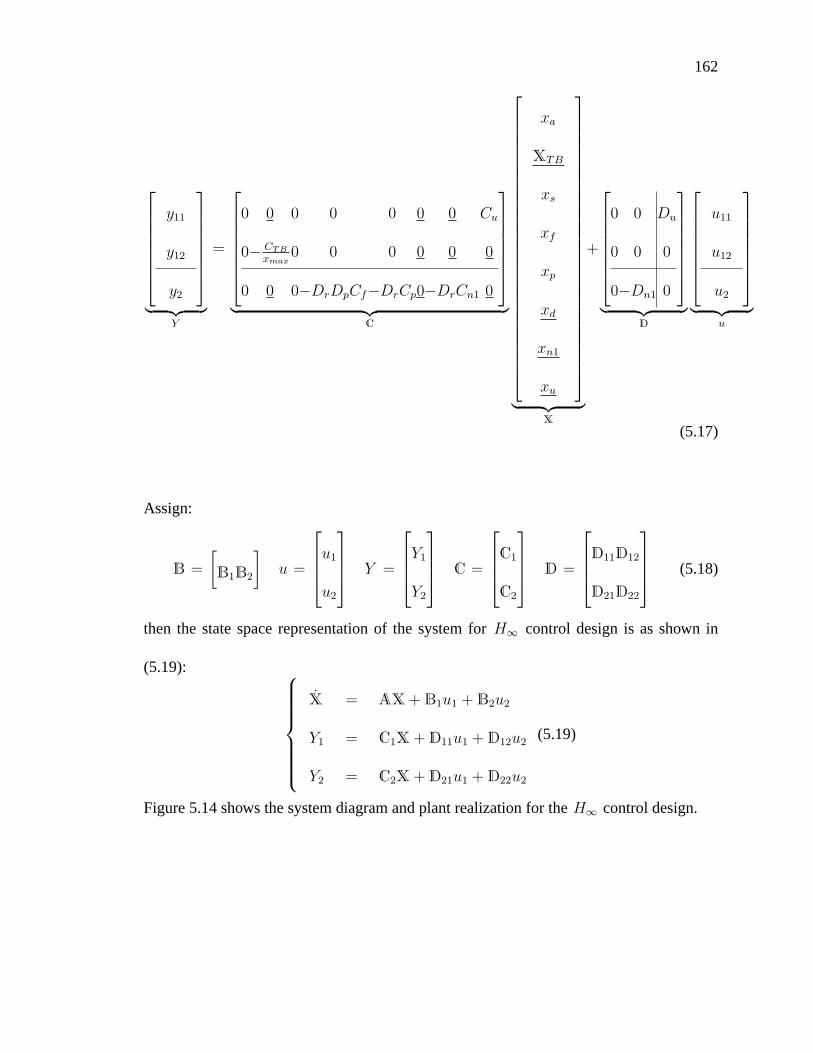
162

y11

y12

y2

︸︷︷︸Y

=

0 0 0 0 0 0 0 Cu

0− CTB

xmax0 0 0 0 0 0

0 0 0−DrDpCf−DrCp0−DrCn1 0

︸︷︷︸C

xa

XTB

xs

xf

xp

xd

xn1

xu

︸︷︷︸X

+

0 0 Du

0 0 0

0−Dn1 0

︸︷︷︸D

u11

u12

u2

︸︷︷︸u

(5.17)

Assign:

B =

[B1B2

]u =

u1

u2

Y =

Y1

Y2

C =

C1

C2

D =

D11D12

D21D22

(5.18)

then the state space representation of the system for H∞ control design is as shown in

(5.19):

X = AX + B1u1 + B2u2

Y1 = C1X + D11u1 + D12u2

Y2 = C2X + D21u1 + D22u2

(5.19)

Figure 5.14 shows the system diagram and plant realization for the H∞ control design.

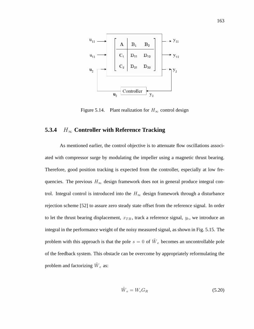
163

Figure 5.14. Plant realization for H∞ control design

5.3.4 H∞ Controller with Reference Tracking

As mentioned earlier, the control objective is to attenuate flow oscillations associ-

ated with compressor surge by modulating the impeller using a magnetic thrust bearing.

Therefore, good position tracking is expected from the controller, especially at low fre-

quencies. The previous H∞ design framework does not in general produce integral con-

trol. Integral control is introduced into the H∞ design framework through a disturbance

rejection scheme [52] to assure zero steady state offset from the reference signal. In order

to let the thrust bearing displacement, xTB , track a reference signal, yt , we introduce an

integral in the performance weight of the noisy measured signal, as shown in Fig. 5.15. The

problem with this approach is that the pole s = 0 of W e becomes an uncontrollable pole

of the feedback system. This obstacle can be overcome by appropriately reformulating the

problem and factorizing W e as:

W e = WeGR (5.20)

164

Figure 5.15. Attempt to introduce integral control in H∞

where GR is proper, containing all the imaginary axis poles of W e , and We is stable and

minimum phase [52]. Now the problem can be formulated in the general LFT framework

as in Fig. 5.16.

Equations (5.21), (5.22) and (5.23) show the state space realization of the weighting func-

tion for the tracking signal, and the integrator.

Tracking Signal Weighting Function W t :

xt = Atxt +Btu13

yt = Ctxt +Dtu13

(5.21)

Gr :

xr = Arxr +Bryh

yr = Crxr +Dryh

(5.22)

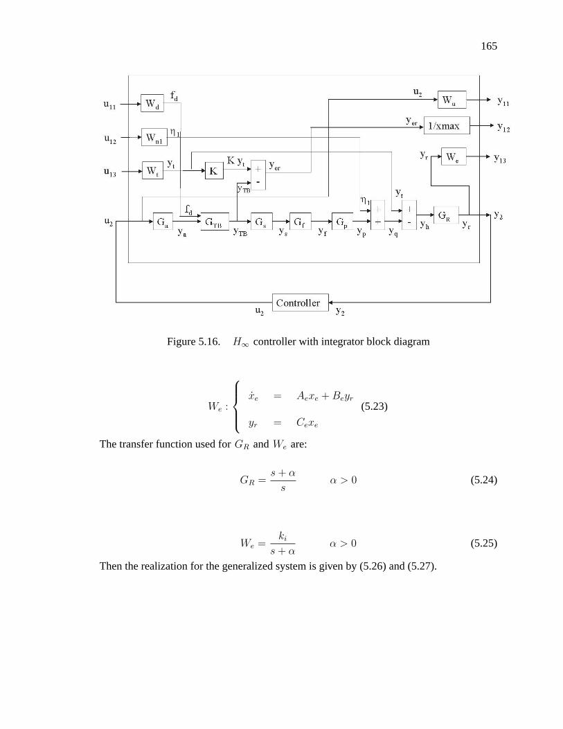
165

Figure 5.16. H∞ controller with integrator block diagram

We :

xe = Aexe +Beyr

yr = Cexe

(5.23)

The transfer function used for GR and We are:

GR =s+ α

sα > 0 (5.24)

We =ki

s+ αα > 0 (5.25)

Then the realization for the generalized system is given by (5.26) and (5.27).

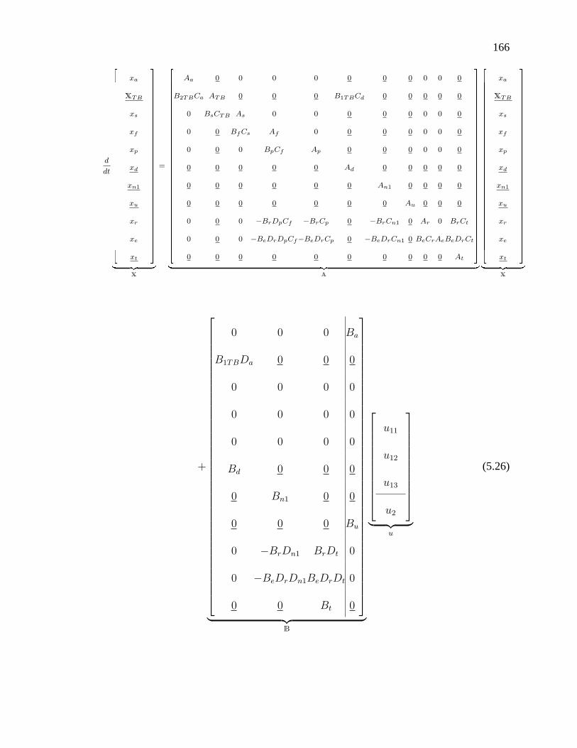
166

d

dt

xa

XTB

xs

xf

xp

xd

xn1

xu

xr

xe

xt

X

=

Aa 0 0 0 0 0 0 0 0 0 0

B2TBCa ATB 0 0 0 B1TBCd 0 0 0 0 0

0 BsCTB As 0 0 0 0 0 0 0 0

0 0 Bf Cs Af 0 0 0 0 0 0 0

0 0 0 BpCf Ap 0 0 0 0 0 0

0 0 0 0 0 Ad 0 0 0 0 0

0 0 0 0 0 0 An1 0 0 0 0

0 0 0 0 0 0 0 Au 0 0 0

0 0 0 −BrDpCf −BrCp 0 −BrCn1 0 Ar 0 BrCt

0 0 0 −BeDrDpCf−BeDrCp 0 −BeDrCn1 0 BeCrAeBeDrCt

0 0 0 0 0 0 0 0 0 0 At

A

xa

XTB

xs

xf

xp

xd

xn1

xu

xr

xe

xt

X

+

0 0 0 Ba

B1TBDa 0 0 0

0 0 0 0

0 0 0 0

0 0 0 0

Bd 0 0 0

0 Bn1 0 0

0 0 0 Bu

0 −BrDn1 BrDt 0

0 −BeDrDn1BeDrDt 0

0 0 Bt 0

︸︷︷︸B

u11

u12

u13

u2

︸︷︷︸u

(5.26)

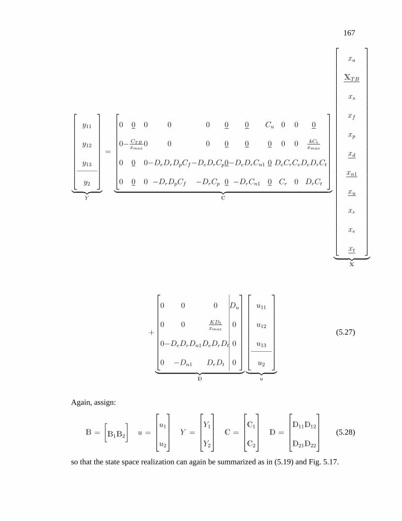
167

y11

y12

y13

y2

︸︷︷︸Y

=

0 0 0 0 0 0 0 Cu 0 0 0

0− CTB

xmax0 0 0 0 0 0 0 0 kCt

xmax

0 0 0−DeDrDpCf−DeDrCp0−DeDrCn1 0 DeCrCeDeDrCt

0 0 0 −DrDpCf −DrCp 0 −DrCn1 0 Cr 0 DrCt

︸︷︷︸C

xa

XTB

xs

xf

xp

xd

xn1

xu

xr

xe

xt

︸︷︷︸X

+

0 0 0 Du

0 0 KDt

xmax0

0−DeDrDn1DeDrDt 0

0 −Dn1 DrDt 0

︸︷︷︸D

u11

u12

u13

u2

︸︷︷︸u

(5.27)

Again, assign:

B =

[B1B2

]u =

u1

u2

Y =

Y1

Y2

C =

C1

C2

D =

D11D12

D21D22

(5.28)

so that the state space realization can again be summarized as in (5.19) and Fig. 5.17.

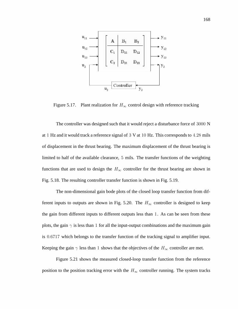
168

Figure 5.17. Plant realization for H∞ control design with reference tracking

The controller was designed such that it would reject a disturbance force of 3000 N

at 1 Hz and it would track a reference signal of 3 V at 10 Hz. This corresponds to 4.28 mils

of displacement in the thrust bearing. The maximum displacement of the thrust bearing is

limited to half of the available clearance, 5 mils. The transfer functions of the weighting

functions that are used to design the H∞ controller for the thrust bearing are shown in

Fig. 5.18. The resulting controller transfer function is shown in Fig. 5.19.

The non-dimensional gain bode plots of the closed loop transfer function from dif-

ferent inputs to outputs are shown in Fig. 5.20. The H∞ controller is designed to keep

the gain from different inputs to different outputs less than 1 . As can be seen from these

plots, the gain γ is less than 1 for all the input-output combinations and the maximum gain

is 0.6717 which belongs to the transfer function of the tracking signal to amplifier input.

Keeping the gain γ less than 1 shows that the objectives of the H∞ controller are met.

Figure 5.21 shows the measured closed-loop transfer function from the reference

position to the position tracking error with the H∞ controller running. The system tracks

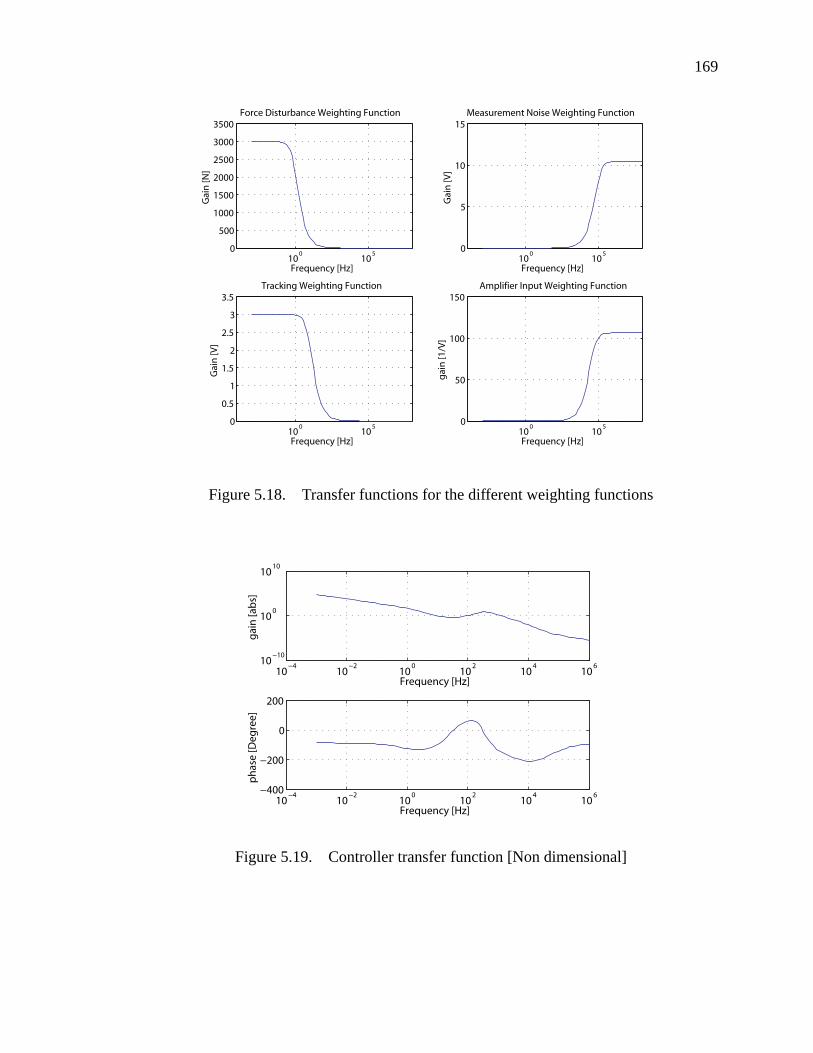
169

100

105

0

500

1000

1500

2000

2500

3000

3500

Gai

n [N

]

Frequency [Hz]

Force Disturbance Weighting Function

100

105

0

5

10

15

Gai

n [V

]

Frequency [Hz]

Measurement Noise Weighting Function

100

105

0

0.5

1

1.5

2

2.5

3

3.5

Gai

n [V

]

Frequency [Hz]

Tracking Weighting Function

100

105

0

50

100

150

gain

[1/V

]Frequency [Hz]

Amplifier Input Weighting Function

Figure 5.18. Transfer functions for the different weighting functions

10−4

10−2

100

102

104

10610

−10

100

1010

gain

[abs

]

Frequency [Hz]

10−4

10−2

100

102

104

106−400

−200

0

200

phas

e [D

egre

e]

Frequency [Hz]

Figure 5.19. Controller transfer function [Non dimensional]

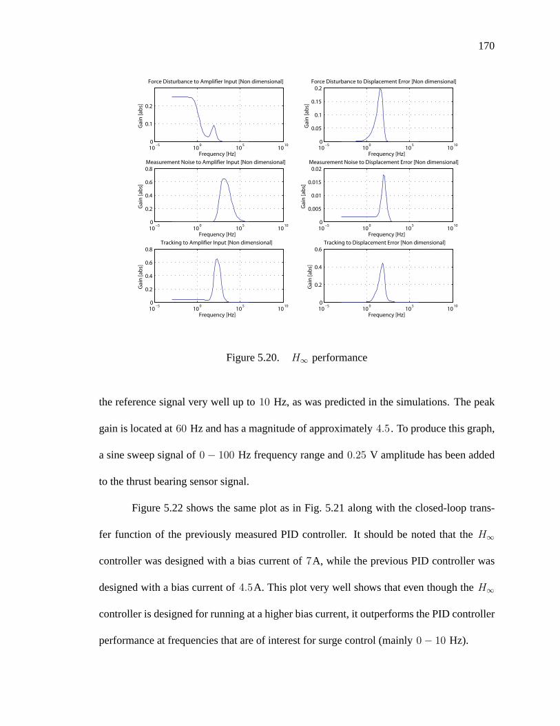
170

10−5

100

105

1010

0

0.1

0.2

Gai

n [a

bs]

Frequency [Hz]

Force Disturbance to Amplifier Input [Non dimensional]

10−5

100

105

1010

0

0.05

0.1

0.15

0.2

Gai

n [a

bs]

Frequency [Hz]

Force Disturbance to Displacement Error [Non dimensional]

10−5

100

105

1010

0

0.2

0.4

0.6

0.8

Gai

n [a

bs]

Frequency [Hz]

Measurement Noise to Amplifier Input [Non dimensional]

10−5

100

105

1010

0

0.005

0.01

0.015

0.02

Gai

n [a

bs]

Frequency [Hz]

Measurement Noise to Displacement Error [Non dimensional]

10−5

100

105

1010

0

0.2

0.4

0.6

0.8

Gai

n [a

bs]

Frequency [Hz]

Tracking to Amplifier Input [Non dimensional]

10−5

100

105

1010

0

0.2

0.4

0.6

Gai

n [a

bs]

Frequency [Hz]

Tracking to Displacement Error [Non dimensional]

Figure 5.20. H∞ performance

the reference signal very well up to 10 Hz, as was predicted in the simulations. The peak

gain is located at 60 Hz and has a magnitude of approximately 4.5 . To produce this graph,

a sine sweep signal of 0 − 100 Hz frequency range and 0.25 V amplitude has been added

to the thrust bearing sensor signal.

Figure 5.22 shows the same plot as in Fig. 5.21 along with the closed-loop trans-

fer function of the previously measured PID controller. It should be noted that the H∞

controller was designed with a bias current of 7A, while the previous PID controller was

designed with a bias current of 4.5A. This plot very well shows that even though the H∞

controller is designed for running at a higher bias current, it outperforms the PID controller

performance at frequencies that are of interest for surge control (mainly 0 − 10 Hz).

171

10−1

100

101

1020

1

2

3

4

5

Gai

n [a

bs]

Frequency [Hz]

Figure 5.21. Measured closed loop transfer function of the H∞ controller

10−1

100

101

1020

1

2

3

4

5

6

Gai

n [a

bs]

Frequency [Hz]

Hinf

PID

Bias current: 7[A]

Bias current: 4.5[A]

Figure 5.22. Comparison between closed loop performance of PID and H∞ controllers

5.4 Radial Bearing Controller

A PID controller is designed for radial levitation of the rotor using active magnetic

bearings. The controller transfer function is:

G(s) =kds+ kp

1ω2ω3s

s2 + ω2+ω3

ω2ω3s+ 1

+ki

swhere kd =

kp

ω1

and ki = kp (5.29)

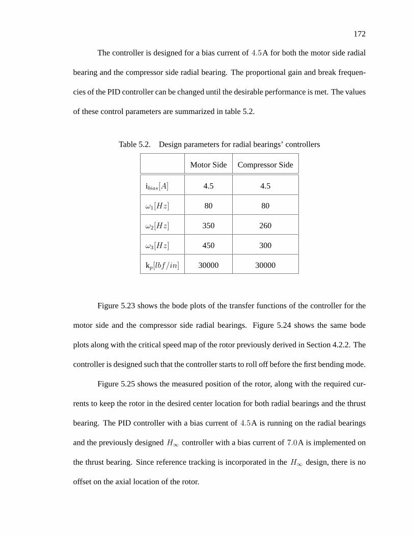
172

The controller is designed for a bias current of 4.5A for both the motor side radial

bearing and the compressor side radial bearing. The proportional gain and break frequen-

cies of the PID controller can be changed until the desirable performance is met. The values

of these control parameters are summarized in table 5.2.

Table 5.2. Design parameters for radial bearings’ controllers

Motor Side Compressor Side

ibias[A] 4.5 4.5

ω1[Hz] 80 80

ω2[Hz] 350 260

ω3[Hz] 450 300

kp[lbf/in] 30000 30000

Figure 5.23 shows the bode plots of the transfer functions of the controller for the

motor side and the compressor side radial bearings. Figure 5.24 shows the same bode

plots along with the critical speed map of the rotor previously derived in Section 4.2.2. The

controller is designed such that the controller starts to roll off before the first bending mode.

Figure 5.25 shows the measured position of the rotor, along with the required cur-

rents to keep the rotor in the desired center location for both radial bearings and the thrust

bearing. The PID controller with a bias current of 4.5A is running on the radial bearings

and the previously designed H∞ controller with a bias current of 7.0A is implemented on

the thrust bearing. Since reference tracking is incorporated in the H∞ design, there is no

offset on the axial location of the rotor.

173

Figure 5.23. PID controller transfer function for motor side and compressor side radial

bearings

100

102

104

10610

2

103

104

105

106

Frequency [rad/sec]

Stiff

ness

[lb/

inch

]

Translational ModeConical ModeFirst Bending ModeSecond Bending ModeRunning Speed

Motor Side Controller

Compresor Side Controller

Figure 5.24. PID controller design for radial bearings

174

−10 −5 0 5 10

−10

−5

0

5

10

Motor side x [mils]

Mot

or s

ide

y [m

ils]

Position

0 0.5 13

4

5

6

Time [sec]

Mot

or s

ide

x [A

]

Amplifier input current

0 0.5 13

4

5

6

Time [sec]

Mot

or s

ide

y [A

]


−10 −5 0 5 10

−10

−5

0

5

10

Compressor side x [mils]

Com

pres

sor s

ide

y [m

ils]

Position

0 0.5 13

4

5

6

Time [sec]

Com

pres

sor s

ide

x [A

] Amplifier input current

0 0.5 13

4

5

6

Time [sec]

Com

pres

sor s

ide

y [A

] Amplifier input current

0 0.5 1

−10

−5

0

5

10

Time [sec]

Thru

st z

[mils

]

Position

0 0.5 16

6.5

7

7.5

8

Time [sec]

Thru

st z

[A]


x1x2

y1y2

x1x2

y1y2

z1z2

Figure 5.25. Measured rotor position and bearing currents with the levitation controller

running: PID for the radial bearings and H∞ for the thrust bearing

5.5 Conclusion

Magnetic levitation of the rotor was established in radial and axial directions. A PID

controller was used for the levitation of the radial bearings. Since the test rig is designed

to be used for testing different surge control algorithm using the magnetic thrust bearing,

an H∞ controller with reference tracking was used for the thrust bearing controller. The

controllers were successfully implemented on the test rig as shown in Fig.5.25.

175

CHAPTER 6

CONCLUSION AND FUTURE RESEARCH

The objectives of the presented work were:

1. To develop a new method for active control of surge in unshrouded centrifugal

compressors using a magnetic thrust bearing as an actuator to modulate the im-

peller blades tip clearance,

2. To develop a test rig that would allow for implementing the proposed surge control

method and could also be used for measuring the impeller and bearing loads at

off–design conditions.

The outcomes of this research are summarized in the following sections.

176

6.1 Conclusion of the Analytical Work

1. A mathematical model was developed to express the effects of tip clearance mod-

ulation on the centrifugal compressor characteristics curve parameters.

2. The existing model for the dynamics of the compression system (Greitzer’s model [22])

was extended to include the influence of dynamic tip clearance modulation.

3. A new method for active control of surge in centrifugal compressors was developed

using tip clearance modulations with a magnetic thrust bearing.

4. The objective of the control design was to keep the system trajectories on the com-

pressor characteristic curve, i.e. the blade tip clearance should be actively modu-

lated with the magnetic thrust bearing, but the mean tip clearance should be kept at

the design value. By ensuring zero steady state offset of the impeller, the intended

efficiency of the compressor is maintained. The performance and efficiency of the

compressor will no longer be sacrificed to control surge.

5. It was shown that it is possible to design a feedback controller based on mass flow

measurements that can stabilize compressor surge and can significantly increase

the stable operating range of the compressor (down to 10% throttle opening in a

typical study).

6. The controller designed based on mass flow feedback assumed infinite actuator

bandwidth and no uncertainties in the throttle settings. Thus, limiting actual imple-

mentation on industrial scale machines and prompting an exploration of alternative

control design strategies.

177

7. It was shown that the sliding mode control method could not be used to force the

state trajectories to follow the steady state compressor characteristic curve due to

the singularity of the resulting controller at the peak of the compressor character-

istic curve and the algebraic difficulties associated with putting the system into the

cascade of integrators canonical form required by sliding mode formulation.

8. This problem was solved using the backstepping control method. The backstep-

ping method also permits inclusion of uncertainties in the throttle setting in the

control synthesis.

9. A backstepping controller without throttle uncertainties was designed with the ob-

jective that system trajectories remain on the compressor characteristic curve in

the presence of disturbances downstream of the compressor which were modeled

as changes in the throttle settings.

10. Results from the simulation of the nonlinear model for a single stage high speed

centrifugal compressor showed that, using backstepping control, mass flow and

pressure oscillations associated with compressor surge were very effectively sup-

pressed and the stable operating range of the compressor was increased signifi-

cantly (down to 10% throttle opening in a typical study, where the passive stable

limit was 52% throttle opening ).

11. Throttle changes producing a reduction in mass flow rate from 60% to 10% in 3

seconds were readily accommodated by the controller with very acceptable im-

peller excursions (less than 15% of the available clearance).

12. To consider the limitations of the conventional magnetic thrust bearings, the thrust

bearing dynamics were included in the synthesis of the backstepping controller. It

178

was shown that it is possible to produce adequate axial excursions using a phys-

ically feasible magnetic thrust bearing with practical levels of drive voltage. The

results showed modest bandwidth requirement for this control method (less than

10 Hz), making the method more attractive to industrial applications.

13. The lack of throttle position knowledge was then properly accommodated in design

of the backstepping control by modeling the throttle settings as uncertainties.

14. Simulation results showed that the compression system can be stabilized in the

presence of downstream disturbances with acceptable impeller tip clearance mod-

ulation (less than 20% of the available clearance for a throttle change from 60%

to 10%). However, this would result in a static offset from the steady state com-

pressor characteristic curve.

15. An integral state was successfully added to the backstepping design to compen-

sate for this static offset and to force the state trajectories follow the steady state

compressor characteristic by requiring a zero steady state impeller excursion.

16. The notion of adding auxiliary integral states to the backstepping problem with

uncertainties appears to be new to the literature and significantly improves the

performance of the backstepping controller in the presence of uncertainties by per-

mitting the control designer extra freedom in choosing the shape of the compact

set to which limit cycles will be confined.

17. The proposed surge control method would allow centrifugal compressors to reli-

ably and safely operate with a wider range than is currently done in the field in the

presence of disturbances.

179

18. Adding the dynamics of the thrust bearing to the backstepping control design in

the presence of uncertainties enormously complicated the algebra associated with

the control synthesis. Therefore, the actual thrust bearing bandwidth requirement

could not be directly established in the presence of throttle uncertainties. Instead, a

more heuristic approach was adopted to assess the impact of uncertainty on band-

width requirements.

19. An upper bound of 80 Hz was estimated for the required actuator bandwidth by

modeling the thrust bearing as a low pass filter and passing the control signal result-

ing from the backstepping design with uncertainties through this low pass filter to

represent the physical limitation of the actual hardware. Inserting the low pass dy-

namics of the thrust actuator did not destabilize the system: the controller worked

well despite the fact that it was designed without these detracting dynamics. This

reinforces the notion that the bandwidth demands of the application are modest

and that physically realized controllers can be expected to be reasonably robust to

unmodeled actuator dynamics.

20. The advantage that this method provides over the conventional surge control meth-

ods is that no additional hardware need be added to the system if the machine is

already equipped with magnetic bearings. Therefore, the compressor performance

and efficiency will no longer sacrificed by excessive recycling to achieve surge

control. The only modification would be in the thrust bearing control algorithm,

thereby minimizing the cost of surge mitigation.

180

6.2 Conclusion of the Experimental Work

1. A high speed centrifugal compressor test rig was developed to be used for imple-

menting different surge control methods and also for measuring the impeller/bearing

loads at off-design conditions.

2. An instrumentation system was developed to monitor the the bearing currents, and

the pressure and temperature throughout the ducts and in the compressor.

3. A modular piping system was designed that permits the use of different plenum

sizes.

4. Tests were performed to identify various components of the rig including the rotor,

bearings, sensor and amplifiers. The measured data were compared to the predicted

component models to assure proper modeling of the system.

5. The component models were used to design a levitating controller for the magnetic

bearing system in radial and axial directions.

6. A PID controller was developed to levitate the rotor using the radial bearings.

7. Since one of the objectives of developing of the test rig is to implement different

surge control algorithms using a magnetic thrust bearing, an H∞ controller with

reference tracking was synthesized for the thrust bearing controller.

8. The controllers were implemented on the test rig and the rotor was successfully

levitated using the magnetic bearings.

181

6.3 Future Research

Upon commissioning of the test rig1, the following experiments should be con-

ducted to produce a working surge control system:

1. Run the fully instrumented machine at different flow conditions to generate the

compressor characteristic map [1]and identify the parameters of the Greitzer model [50].

2. Investigate the validity of the derived tip clearance model as described in Sec-

tion 2.8. With the test rig commissioned, the validity of this model can be inves-

tigated by measuring the locally linearized dynamics between axial displacement

and pressure response. This dynamic can be measured freely in the stable oper-

ating regime of the compressor and compared directly to model predictions. The

expectation is that, as the throttle opening is decreased toward surge, the trans-

fer function from tip clearance to pressure ratio will exhibit a progressively less

damped peak.

3. Pressure measurements are more readily available in practice than mass flow mea-

surements. Also, pressure sensors usually have wider bandwidths than flow sen-

sors. Therefore, mass flow rates should be estimated from pressure measurements:

some work needs to be done to develop the math for this estimator and to ensure

that estimator dynamics do not conflict with the backstepping controllers. To check

the accuracy of the estimation process, the estimated values from steady operation

can be compared to steady measurements from an orifice meter which should be

mounted in the piping system.

1See Appendix E for details

182

4. Implement the mass flow feedback surge controller. Using the mass flow feed-

back controller, the stable operating range of the compressor would extend signif-

icantly. However, this controller would not accommodate for the uncertainties in

the throttle settings. An objective here is to establish a baseline against which the

backstepping control will be evaluated.

5. Theoretically, the nonlinear backstepping controller would allow for stabilization

of the entire compressor characteristic curve in the presence of disturbances down-

stream the compressor. First, a backstepping surge controller should be imple-

mented assuming knowledge of the throttle setting. The throttle opening should

vary with the controller running to establish the actual achievable stable range of

operation.

6. Uncertainties in the throttle setting should be included in the implementation of

the surge controller to investigate the robustness of the method to disturbances

downstream of the compressor.

APPENDIX A

BACKSTEPPING CALCULATIONS

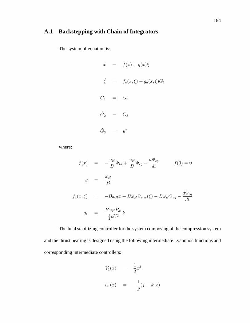
184

A.1 Backstepping with Chain of Integrators

The system of equation is:

x = f(x) + g(x)ξ

ξ = fa(x, ξ) + ga(x, ξ)G1

G1 = G2

G2 = G3

G3 = u∗

where:

f(x) = −ωH

BΦth +

ωH

BΦeq − dΨeq

dtf(0) = 0

g =ωH

B

fa(x, ξ) = −BωHx+BωHΨc,ss(ξ) −BωHΨeq − dΦeq

dt

g1 =BωHPo1

12ρU2

k

The final stabilizing controller for the system composing of the compression system

and the thrust bearing is designed using the following intermediate Lyapunoc functions and

corresponding intermediate controllers:

V1(x) =1

2x2

α1(x) = −1

g(f + k0x)

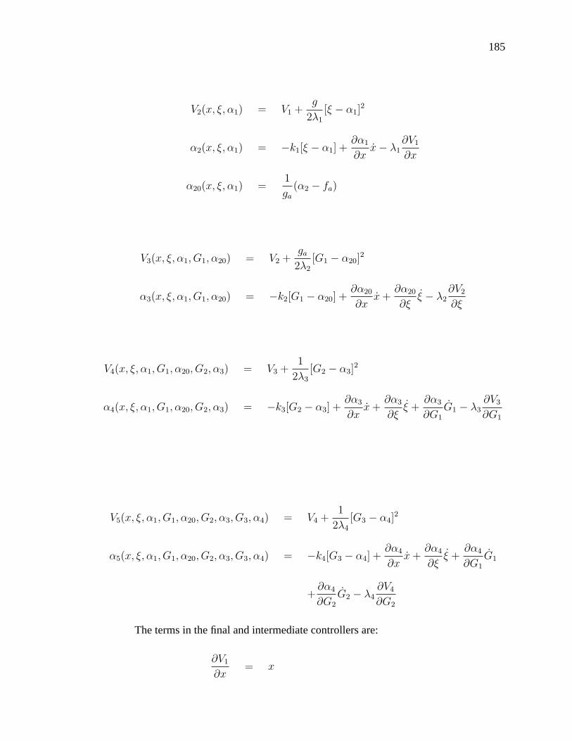
185

V2(x, ξ, α1) = V1 +g

2λ1

[ξ − α1]2

α2(x, ξ, α1) = −k1[ξ − α1] +∂α1

∂xx− λ1

∂V1

∂x

α20(x, ξ, α1) =1

ga

(α2 − fa)

V3(x, ξ, α1, G1, α20) = V2 +ga

2λ2

[G1 − α20]2

α3(x, ξ, α1, G1, α20) = −k2[G1 − α20] +∂α20

∂xx+

∂α20

∂ξξ − λ2

∂V2

∂ξ

V4(x, ξ, α1, G1, α20, G2, α3) = V3 +1

2λ3

[G2 − α3]2

α4(x, ξ, α1, G1, α20, G2, α3) = −k3[G2 − α3] +∂α3

∂xx+

∂α3

∂ξξ +

∂α3

∂G1

G1 − λ3∂V3

∂G1

V5(x, ξ, α1, G1, α20, G2, α3, G3, α4) = V4 +1

2λ4

[G3 − α4]2

α5(x, ξ, α1, G1, α20, G2, α3, G3, α4) = −k4[G3 − α4] +∂α4

∂xx+

∂α4

∂ξξ +

∂α4

∂G1

G1

+∂α4

∂G2

G2 − λ4∂V4

∂G2

The terms in the final and intermediate controllers are:

∂V1

∂x= x

186

∂α1

∂x= −1

g

(∂f

∂x+ k0

)

∂f

∂x= −ωH

B

∂Φth

∂x=

−ωHcthuth

2B√x+ Ψeq

∂α20

∂x=

1

ga

(∂α2

∂x− ∂fa

∂x

)

∂α2

∂x= k1

∂α1

∂x+∂2α1

∂2xx+

∂α1

∂x

∂

∂xx− ∂2V1

∂2xg

∂2α1

∂x2= −1

g

∂2f

∂2x

∂2f

∂x2=

ωHcthuth

4B(x+ Ψeq)32

∂

∂xx =

∂

∂x(f + gξ) =

∂f

∂x

∂2V1

∂x2= 1

∂fa

∂x= −BωH

∂α20

∂ξ=

1

ga

(∂α2

∂ξ− ∂fa

∂ξ

)

∂α2

∂ξ= −k1 +

∂α1

∂x

∂

∂ξx

∂

∂ξx =

∂

∂ξ(f + gξ) = g

∂fa

∂ξ=

BωHPo1

12ρU2

[3A1(ξ + Φeq)2 + 2B1(ξ + Φeq) + C1]

187

∂α3

∂x= k2

∂α20

∂x+

∂

∂x

∂α20

∂xx+

∂α20

∂x

∂

∂xx+

∂

∂x

∂α20

∂ξξ +

∂α20

∂ξ

∂

∂xξ − λ2

∂

∂x

∂V2

∂ξ

∂

∂x

∂α20

∂x=

1

ga

(∂2α2

∂x2− ∂2fa

∂x2

)=

1

ga

∂2α2

∂x2

∂2α2

∂x2= k1

∂2α1

∂x2+∂3α1

∂x3x+ 2

∂2α1

∂x2

∂

∂xx+

∂α1

∂x

∂2

∂x2x− ∂3V1

∂x3g

∂3α1

∂x3= −1

g

∂3f

∂x3

∂3f

∂x3=

−3ωHcthuth

8B(x+ Ψeq)52

∂2

∂x2x =

∂

∂x

∂f

∂x=∂2f

∂x2

∂3V1

∂x3= 0

∂

∂x

∂α20

∂ξ=

1

ga

(∂

∂x

∂α2

∂ξ− ∂

∂x

∂fa

∂ξ

)=

1

ga

∂

∂x

∂α2

∂ξ

∂

∂x

∂α2

∂ξ=

∂2α1

∂x2

∂

∂ξx+

∂α1

∂x

∂

∂x

∂

∂ξx

∂

∂x

∂

∂ξx = 0

∂

∂xξ =

∂

∂x(fa + gaG1) =

∂fa

∂x

∂

∂x

∂V2

∂ξ=

g

λ1

∂

∂x(ξ − α1) = − g

λ1

∂α1

∂x

∂α3

∂ξ= k2

∂α20

∂ξ+

∂

∂ξ

∂α20

∂xx+

∂α20

∂x

∂

∂ξx+

∂2α20

∂ξ2ξ +

∂α20

∂ξ

∂

∂ξξ − ∂2V2

∂ξ2

∂

∂ξ

∂α20

∂x=

1

ga

(∂

∂ξ

∂α2

∂x− ∂

∂ξ

∂fa

∂x

)=

1

ga

∂

∂ξ

∂α2

∂x

∂

∂ξ

∂α2

∂x=

∂2α1

∂x2

∂

∂ξx

188

∂2α20

∂ξ2=

1

ga

(∂2α2

∂ξ2− ∂2fa

∂ξ2

)

∂2α2

∂ξ2=

∂

∂ξ

∂α1

∂x

∂

∂ξx+

∂α1

∂x

∂2

∂ξ2x

∂

∂ξ

∂α1

∂x= 0

∂2

∂ξ2x = 0

∂2fa

∂ξ2=

BωHPo1

12ρU2

[6A1(ξ + Φeq) + 2B1]

∂

∂ξξ =

∂

∂ξ(fa + gaG1) =

∂fa

∂ξ

∂2V2

∂ξ2=

g

λ1

∂

∂ξ(ξ − α1) =

g

λ1

∂α3

∂G1

= −k2 +∂α20

∂ξ

∂

∂G1

ξ

∂

∂G1

ξ =∂

∂G1

(fa + gaG1) = ga

∂α4

∂ξ= k3

∂α3

∂ξ+

∂

∂ξ

∂α3

∂xx+

∂α3

∂x

∂

∂ξx+

∂2α3

∂ξ2ξ +

∂α3

∂ξ

∂

∂ξξ +

∂2α3

∂ξ∂G1

G1

+∂α3

∂G1

∂

∂ξG1 − ∂

∂ξ

∂V3

∂G1

∂

∂ξ

∂α3

∂x= k2

∂2α20

∂ξ∂x+

∂

∂ξ

∂2α20

∂x2x+

∂2α20

∂x2

∂

∂ξx+

∂2α20

∂ξ∂x

∂

∂xx+

∂α20

∂x

∂2

∂ξ∂xx

+∂

∂ξ

∂2α20

∂x∂ξξ +

∂2α20

∂x∂ξ

∂

∂ξξ +

∂2α20

∂ξ2

∂

∂xξ +

∂α20

∂ξ

∂2

∂ξ∂xξ − ∂

∂ξ

∂2V2

∂ξ∂x

∂

∂ξ

∂2α20

∂x2=

1

ga

∂

∂ξ

∂2α2

∂x2=

1

ga

∂3α1

∂x3

∂

∂ξx

189

∂2

∂ξ∂xx =

∂

∂ξ

∂f

∂x= 0

∂

∂ξ

∂2α20

∂x∂ξ=

∂

∂ξ

[1

ga

∂2α1

∂x2

∂fa

∂x

]= 0

∂2

∂ξ∂xξ =

∂

∂ξ

∂fa

∂x= 0

∂

∂ξ

∂2V2

∂ξ∂x= − g

λ1

∂

∂ξ

∂α1

∂x= 0

∂2α3

∂ξ2= k2

∂2α20

∂ξ2+

∂

∂ξ

∂2α20

∂ξ∂xx+ 2

∂2α20

∂ξ∂x

∂

∂ξx+

∂α20

∂x

∂2

∂ξ2x+

∂3α20

∂ξ3ξ

+2∂2α20

∂ξ2

∂

∂ξξ +

∂α20

∂ξ

∂2

∂ξ2ξ − ∂3V2

∂ξ3

∂

∂ξ

∂2α20

∂ξ∂x=

1

ga

∂

∂ξ

(∂2α1

∂x2

∂

∂ξx

)=

1

ga

∂2α1

∂x2

∂2

∂ξ2x = 0

∂3α20

∂ξ3= − 1

ga

∂3fa

∂ξ3

∂3fa

∂ξ3= 6A1

BωHPo1

12ρU2

∂2

∂ξ2ξ =

∂

∂ξ

∂fa

∂ξ=∂2fa

∂ξ2=BωHPo1

12ρU2

[6A1(ξ + Φeq) + 2B1]

∂3V2

∂ξ3= 0

∂2α3

∂ξ∂G1

=∂

∂ξ(−k2 + ga

∂α20

∂ξ) = ga

∂2α20

∂ξ2

∂

∂ξG1 = 0

∂

∂ξ

∂V3

∂G1

=∂

∂ξ(ga

λ2

(G1 − α20)) = −ga

λ2

∂α20

∂ξ

190

∂α4

∂x= k3

∂α3

∂x+∂2α3

∂x2x+

∂α3

∂x

∂

∂xx+

∂2α3

∂x∂ξξ +

∂α3

∂ξ

∂

∂xξ +

∂2α3

∂x∂G1

G1

+∂α3

∂G1

∂

∂xG1 − ∂

∂x

∂V3

∂G1

∂2α3

∂x2= k2

∂2α20

∂x2+∂3α20

∂x3x+ 2

∂2α20

∂x2

∂

∂xx+

∂α20

∂x

∂2

∂x2x+

∂

∂x

∂2α20

∂x∂ξξ

+2∂2α20

∂x∂ξ

∂

∂xξ +

∂α20

∂ξ

∂2

∂x2ξ − ∂2

∂x2

∂V2

∂ξ

∂3α20

∂x3=

1

ga

∂3α2

∂x3

∂3α2

∂x3= k1

∂3α1

∂x3+∂4α1

∂x4x+ 3

∂3α1

∂x3

∂

∂xx+ 3

∂2α1

∂x2

∂2

∂x2x+

∂α1

∂x

∂3

∂x3x

∂4α1

∂x4= −1

g

∂4f

∂x4

∂4f

∂x4=

15ωHcthuth

16B(x+ Ψeq)72

∂3

∂x3x =

∂3f

∂x3

∂

∂x

∂2α20

∂ξ∂x=

∂

∂x

[1

ga

∂2α1

∂x2

∂

∂ξx

]=

1

ga

∂3α1

∂x3

∂

∂ξx

∂2

∂x2ξ =

∂

∂x

∂fa

∂x=∂2fa

∂x2= 0

∂2

∂x2

∂V2

∂ξ= − g

λ1

∂2α1

∂x2

∂2α3

∂x∂G1

=∂

∂x(−k2 + ga

∂α20

∂ξ) = ga

∂2α20

∂x∂ξ

∂

∂xG1 = 0

∂

∂x

∂V3

∂G1

=∂

∂x(ga

λ2

(G1 − α20)) = −ga

λ2

∂α20

∂x

191

∂α4

∂G1

= k3∂α3

∂G1

+∂

∂G1

∂α3

∂xx+

∂α3

∂x

∂

∂G1

x+∂

∂G1

∂α3

∂ξξ +

∂α3

∂ξ

∂

∂G1

ξ +∂2α3

∂G21

G1

+∂α3

∂G1

∂

∂G1

G1 − ∂2V3

∂G21

∂

∂G1

∂α3

∂x=

∂2α20

∂x∂ξ

∂

∂G1

ξ +∂α20

∂ξ

∂

∂G1

∂ξ

∂x

∂

∂G1

ξ = ga

∂

∂G1

∂ξ

∂x= 0

∂

∂G1

x = 0

∂

∂G1

∂α3

∂ξ=

∂2α20

∂ξ2

∂

∂G1

ξ +∂α20

∂ξ

∂

∂G1

∂ξ

∂ξ

∂

∂G1

∂ξ

∂ξ= 0

∂2α3

∂2G1

=∂

∂G1

(−k2 + ga∂α20

∂ξ) = 0

∂

∂G1

G1 =∂

∂G1

G2 = 0

∂2V3

∂G21

=ga

λ2

∂

∂G1

(G1 − α1) =ga

λ2

∂α4

∂G2

= −k3 +∂α3

∂G1

∂

∂G2

G1

∂

∂G2

G1 =∂

∂G2

G2 = 1

A.2 Backstepping with Uncertainties

The system of equation is:

192

x =ωH

B

(ξ − cth(A2x+B2)∆3 − cthA2∆4 + ∆2 − B

ωH

∆7

)

ξ = BωH

(f2a(x, ξ) +

1

BωH

gaG1 +3Po1A1

12ρU2

ξ2∆2 +Po1

12ρU2

ξ∆5 +Po1

12ρU2

∆6 − ∆1 − 1

BωH

∆8

)

where:

The intermediate Lyapunov functions and corresponding intermediate controllers

are:

V1(x) =B

2ωH

x2

ξ = α1(x) = −σ1x− k1x

[1 + (cth(A2x+B2))

2 + (cthA2)2 +

(B

ωH

)2]

V2(x, ξ, α1) = V1 +1

2λ1BωH

[ξ − α1]2

G0

BωH

=α2(x, ξ)

BωH

= −σ2[ξ − α1] − λ1x+1

B2

∂α1

∂xξ − k2

λ1

[ξ − α1]

[1

(BωH)2

+

(3Po1A1

12ρU2

ξ2

)2(Po1

12ρU2

ξ

)2

+

(Po1

12ρU2

)2

+ 1 +

(1

B2

∂α1

∂xcth(A2x+B2)

)2

+

(1

B2

∂α1

∂xcthA2

)2

+

(1

B2

∂α1

∂x

)2

+

(1

BωH

∂α1

∂x

)2]

G1 = α20(x, ξ, α1) =1

ga

(α2 −BωHf2a)

APPENDIX B

VARIABLE FREQUENCY DRIVE SETTINGS

APPENDIX C

AMPLIFIER IDENTIFICATION

196

Figures C.1-C.10 show the measured gains on the amplifiers and the current moni-

tors. The amplifier gain is roughly 1.5[A/V] and the average current monitor gain is about

5[A/V].

y = 1.4999x + 0.0004R2 = 1.0000

-2.0000

-1.0000

0.0000

1.0000

2.0000

-1.500 -1.000 -0.500 0.000 0.500 1.000 1.500

Input Voltage [V]

Out

put C

urre

nt [A

]

y = 4.9281x - 0.0111R2 = 1.0000

-2.0000

-1.0000

0.0000

1.0000

2.0000

-0.400 -0.200 0.000 0.200 0.400

Current Monitor [V]

Out

put C

urre

nt [A

]

Figure C.1. Calibration of amplifier #1, Left: current monitor gain, Right: amplifier gain

y = 4.9080x - 0.0227R2 = 1.0000

-2.0000

-1.0000

0.0000

1.0000

2.0000

-0.400 -0.200 0.000 0.200 0.400

Current Monitor [V]

Out

put C

urre

nt [A

y = 1.5039x - 0.0016R2 = 1.0000

-2.0000

-1.0000

0.0000

1.0000

2.0000

-1.500 -1.000 -0.500 0.000 0.500 1.000 1.500

Input Voltage [V]

Out

put C

urre

nt [A


197

y = 4.9114x + 0.0203R2 = 1.0000

-2.0000

-1.0000

0.0000

1.0000

2.0000

-0.400 -0.200 0.000 0.200 0.400

Current Monitor [V]

Out

put C

urre

nt [A

y = 1.4975x + 0.0014R2 = 1.0000

-2.0000

-1.0000

0.0000

1.0000

2.0000

-1.500 -1.000 -0.500 0.000 0.500 1.000 1.500

Input Voltage [V]

Out

put C

urre

nt [A


y = 4.9341x - 0.0278R2 = 1.0000

-2.0000

-1.0000

0.0000

1.0000

2.0000

-0.400 -0.200 0.000 0.200 0.400

Current Monitor [V]

Out

put C

urre

nt [A

y = 1.5023x - 0.0017R2 = 1.0000

-2.0000

-1.0000

0.0000

1.0000

2.0000

-1.500 -1.000 -0.500 0.000 0.500 1.000 1.500

Input Voltage [V]

Out

put C

urre

nt [A


y = 4.9177x - 0.0079R2 = 1.0000

-2

-1

0

1

2

-0.400 -0.200 0.000 0.200 0.400

Current Monitor [V]

Out

put C

urre

nt [A

y = 1.5010x + 0.0006R2 = 1.0000

-2

-1

0

1

2

-1.500 -1.000 -0.500 0.000 0.500 1.000 1.500

Input Voltage [V]

Out

put C

urre

nt [A


198

y = 4.9437x - 0.0035R2 = 1.0000

-2.0000

-1.0000

0.0000

1.0000

2.0000

-0.400 -0.200 0.000 0.200 0.400

Current Monitor [V]

Out

put C

urre

nt [A

y = 1.4974x + 0.0008R2 = 1.0000

-2.0000

-1.0000

0.0000

1.0000

2.0000

-1.500 -1.000 -0.500 0.000 0.500 1.000 1.500

Input Voltage [V]

Out

put C

urre

nt [A


y = 4.9066x - 0.0136R2 = 1.0000

-2.0000

-1.0000

0.0000

1.0000

2.0000

-0.400 -0.200 0.000 0.200 0.400

Current Monitor [V]

Out

put C

urre

nt [A

y = 1.4999x - 0.0017R2 = 1.0000

-2.0000

-1.0000

0.0000

1.0000

2.0000

-1.500 -1.000 -0.500 0.000 0.500 1.000 1.500

Input Voltage [V]

Out

put C

urre

nt [A


y = 4.8713x - 0.0165R2 = 0.9998

-2.0000

-1.0000

0.0000

1.0000

2.0000

-0.400 -0.200 0.000 0.200 0.400

Current Monitor [V]

Out

put C

urre

nt [A

y = 1.5004x + 0.0002R2 = 1.0000

-2.0000

-1.0000

0.0000

1.0000

2.0000

-1.500 -1.000 -0.500 0.000 0.500 1.000 1.500

Input Voltage [V]

Out

put C

urre

nt [A


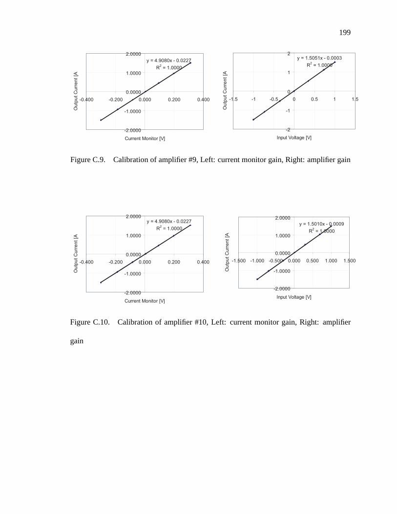
199

y = 4.9080x - 0.0227R2 = 1.0000

-2.0000

-1.0000

0.0000

1.0000

2.0000

-0.400 -0.200 0.000 0.200 0.400

Current Monitor [V]

Out

put C

urre

nt [A

y = 1.5051x - 0.0003R2 = 1.0000

-2

-1

0

1

2

-1.5 -1 -0.5 0 0.5 1 1.5

Input Voltage [V]

Out

put C

urre

nt [A


y = 4.9080x - 0.0227R2 = 1.0000

-2.0000

-1.0000

0.0000

1.0000

2.0000

-0.400 -0.200 0.000 0.200 0.400

Current Monitor [V]

Out

put C

urre

nt [A

y = 1.5010x - 0.0009R2 = 1.0000

-2.0000

-1.0000

0.0000

1.0000

2.0000

-1.500 -1.000 -0.500 0.000 0.500 1.000 1.500

Input Voltage [V]

Out

put C

urre

nt [A

Figure C.10. Calibration of amplifier #10, Left: current monitor gain, Right: amplifier

gain

APPENDIX D

INSTRUCTIONS TO OPERATE THE CONTROLLER

201

To run the controller for magnetic bearings follow these instructions:

1. Start the computer, choose RTLinux from the boot menu

2. Username: guest

3. Password: romacguest

4. From the taskbar click on the terminal icon (to the right of the red hat, computer

screen icon)

5. Become super user. Type: su and use Password: lAyton1

6. Type: cd /home/ds5bf/Control/rtControl

7. Start the realtime task. Type: rtlinux start rttask

8. Turn on the control rack

9. Put Master Enable to ON position (on the Control Rack)

10. Load a controller. Type: ./control/l/cPID − AllLev.m

11. Follow the menu options

12. To turn on the controller choose the menu number 1 (state) by typing 1 . Type: 1

to turn on the controller and type: 0 to turn off the controller

13. To get out of each menu type: −1

14. To stop the realtime task, type: rtlinux stop rttask

15. To monitor the currents and positions open another terminal from the taskbar

16. Become super user (follow the step 5)

17. Type: cd /home/ds5bf/Control/rtControl

18. Type: ./spy 3 (shows the last 3 samples, you can play with the number of samples

to monitor)

19. To stop the controller at any time press the red switch on the Control Rack

202

20. To see what RTLinux packages are running type: rtlinux status

APPENDIX E

INSTRUCTIONS FOR COMMISSIONING THE TEST RIG

204

The following tasks should be performed to make the test rig ready for conducting experi-

ments:

1. Reassemble the test section with the repaired bearing/rotor.

2. Calibrate the new position sensors for the compressor side radial bearing.

3. Recalibrate the axial position sensors using a reference eddy current sensor to re-

duce hysteresis effects.

4. Reestablish magnetic levitation with the new position sensors.

5. Remove the motor shaft hub and measure the shaft and hub runouts.

6. Reassemble the coupling hub on the motor shaft assuring runout of less than

2 mils.

7. Allign the motor shaft with the compressor shaft using Rim-and-Face method.

8. Set up remote computer system using Secure CRT and a local network: test remote

rotor leviation and motor start/stop.

9. Install the motor/bearings cooling system.

10. Run the open face compressor (without the stationary shroud) to assure safe initial

spin-up and measure the vibration and temperature levels.

11. Install pressure and temperature probes in the inlet/exhaust ducts according to [1].

12. Install the shroud and inlet/exhaust pipes. Recheck the alignment of the shafts after

adding each component [3].

13. Follow PTC [1] instructions and contact KOBE Steel before running the machine

at full speed.

205

REFERENCES

1. ASME, Performance Test Code on Compressors and Exhausters. PTC 10-1997,

American Society of Mechanical Engineers, 7th ed., 1998.

2. Barabanov M. and Yodaiken V., Real-Time Linux, Linux Journal, March 1996.

3. Bloch H. P. and Geitner F. K., Practical Machinery Managment for Process Plants,

Volume 3, Second Edition, Machinery Component Maintenance and Repair, Golf

Publishing Company, 1990.

4. Botros K. K., and Henderson J. F., Development in Centrifugal Compressor Surge

Control- A Technology Assessment, Journal of Turbomachinery, Vol. 116, pp. 240-

249, 1994.

5. Boyce M. P., Gas Turbine Engineering Handbook, Gulf Publishing Company, 1982.

6. Brown, N. K., High-speed Compressor Facility–Electromechaniacal Design, Mas-

ter’s Thesis, Department of Mechanical and Aerospace Engineering, University of

Virginia, 2005.

206

7. Buskirk E.S., Sanadgol D., Maslen, E.H. and Brown N., Centrifugal Compressor

Test Facility with Active Magnetic Bearings, The Ninth International Symposium on

Magnetic Bearings, 2004.

8. Christensen D. M., Developing a Characteristic Compressor Curve for a High-Speed

Centrifugal Compressor, Undergraduate Thesis Project, Department of Mechanical

and Aerospace Engineering, University of Virginia, 2006.

9. Childs D., Turbomachinery Rotordynamics: Phenomena, Modeling, And Analysis,

Wiley-Interscience, 1993.

10. Chiu J., Cooling The High-Speed Induction Motor Of An Air Compression System,

Undergraduate Thesis Project, Department of Mechanical and Aerospace Engineer-

ing, University of Virginia, 2006.

11. Cumpsty N. A., Compressor Aerodynamics, Longman Scientific Technical, 1989.

12. de Jager B., Rotating Stall and Surge Control: A Survey, Proceedings of the 34th

Conference on Decision and Control, New Orleans, LA, pp 1857-1862, 1995.

13. Eisenlohr G and Chladek H, Thermal Tip Clearance Control for Centrifugal Comres-

sor of an APU Engine, Journal of Turbomachinery, Vol. 116, pp. 629-634, 1994.

14. Epstein A. H., Ffows Williams J. E. and Greitzer E. M., Active Supression of Aero-

dynamic Instabilities in Turbomachines, Journal of Propulsion, Vol. 5, pp. 204-211,

1989.

15. Emmons H. W., Pearson C. E. and Grant H. P., Compressor Surge and Stall Propaga-

tion, Transactions of the ASME, pp 455-469, 1955.

16. Ffows Williams and Huang X. Y., Active Stabilization of Compressor Surge, Journal

of Fluid Mechanics, Vol. 204, pp. 245-262, 1989.

207

17. Fink D. A., Cumpsty N. A. and Greitzer E. M., Surge Dynamics in a Free-Spool

Centrifugal Compressor System, Journal of Turbomachinery, Vol. 114, pp 321-332,

1992.

18. FSM Labs Inc., Getting Started with RTLinux, 2001.

19. Graf M. B., Wong T. S., Greitzer E. M., Marble F. E., Tan C. S., Shin H. W. and Wisler

D.C., Effects of Nonaxisymmetric Tip Clearance on Axial Compressor Performance

and Stability, Journal of Turbomachinery, Vol. 120, pp 661-648, 1998.

20. Gravdahl J.T., Egeland O. and Vatland S.O., Active Surge Control of Centrifugal Com-

pressors Using Drive Torque, Proceedings of 40th IEEE Conference on Decision and

Control, pp 1286-1291, 2001.

21. Gravdahl J.T., Egeland O., 1999, Compressor Surge and Rotating Stall, Springer.

22. Greitzer E. M., Surge and Rotating Stall in Axial Flow Compressors, Parts I, II,

ASME Journal of Engineering for Power, Vol. 120, pp 190-217, 1976.

23. Greitzer E. M., Review-Axial Compressor Stall Phenomena, ASME Journal of Fluids

Engineering, Vol. 102, pp 134-151, 1980.

24. Greitzer E. M. and Moore F. K., A Theory of Post-Stall Transients in Axial Com-

pressor Systems, Journal of engineering for Gas Turbines and Power, Vol. 108, pp

231-239, 1986.

25. Gysling D. L., Dugundji J., Greitzer E. M., and Epstein A H., Dynamic control of

centrifugal compressor surge using tailored structures, Journal of Turbomacbinery,

Vol. 113, pp. 710-7722, 1991.

26. Hansen K. E., Jorgensen P. and Larsen P. S., Experimental and Theoretical Study of

Surge in a Small Centrifugal Compressor, ASME Journal Fluids Engineering, Vol.

208

103, pp 391-395, 1981.

27. The Fundamentals of Modal Testing, Application Note 243-3, Hewlett Packard.

28. Iura T. and Rannie W. D., Experimental Investigations of Propagating Stall in Axial-

Flow Compressors, ASME Transaction, pp 463-471, 1954.

29. Hewlett Packard, The fundamentals of Modal Testing, Application Note 243-3,

http://www.agilnet.com, 2000.

30. Khalil, H. K., Nonlinear Systems, Prentice-Hall, Inc, 1996.

31. Krstic, M., Kanellakopoulos, I. and Kokotovic, P., Nonlinear and Adaptive Control

Design, Wiley-Interscience, 1995.

32. L. Lamport, LATEX: A document preparation system, 2nd ed., Addison-Wesley, New

York, 1994.

33. Mansoux C. A., Gysling D. L., Setiawan J. D., Paduano J. D., Distributed Nonlinear

Modeling and Stability Analysis of Axial Compressors, Proceedings of the American

Control Conference, pp 2305-2316, 1994.

34. Maresca R. L., A general method for designing low-temperature drift, high-

bandwidth, variable-reluctance position sensors, IEEE Transactions on Magnetics,

vol. 22, pp. 118-123, 1986.

35. Marquez H. J., Nonlinear Control Systems, Analysis and Design, Wiley-Interscience,

2003.

36. Maslen, E. H., Sortore, C. K. and Meeker D. , Analysis Software for Magnetic Bear-

ing Audits, ROMAC Report No. 406, School of Engineering and Applied Science,

Department of Mechanical Engieering, University of Virginia, 2000.

209

37. McKee R. J., Edlund C. E. and Pantermuehl P. J., Development of an Active Surge

Control System, Gas Machinery Research Council, Report No. TR 00-3, 2000.

38. Pampreen R. C., Trans. ASME, Ser. A, Vol. 95, No. 3 (1973-7), p.251,

39. Pinsley J. E., Guenette G. R., Epstein A. H., and Greitzer E. M., Active Stabilization

of Centrifugal Compressor Surge, Journal of Turbomachinery, Vol. 113, pp. 723-732,

1991.

40. Piotrowski J., Shaft alignment handbook, M. Dekker, 1995.

41. Schweitzer G, Bleuler H and Traxler A, Active Magnetic Bearings, vdf Hochschul-

verlag AG, 1994.

42. Senoo Y., Pressure Losses and Flow Field Distortion Induced by Tip Clearance of

Centrifugal and Axial Compressors, JSME International Journal, Vol. 30, No. 261,

pp 375-385, 1987.

43. Senoo Y. and Ishida M., Deterioration of Comressor Performance Due to Tip Clear-

ance of Centrifugal Impellers, Journal of Turbomachinery, Vol. 109, pp 55-61, 1987.

44. Sepulchre R., Kokotovi P., Shape Signifiers of Throttle Control of a Low Order Com-

pressor Model, 1996.

45. Slotine, J-J. E. and Li, W., Applied Nonlinear Control, Prentice-Hall, Englewood

Cliffs, NJ, 1991.

46. Spakovsky Z.S., Paduano J.D., Larsonneur R., Traxler A. and Bright M. M., Tip

Clearance Actuation with Magnetic Bearing For High Speed Compressor Stall Con-

trol, ASME Turbo Expo 2000.

47. VibrAlign Inc, Precision Shaft Alignment, Reference Guide, VibrAlign Inc, 1997.

210

48. Wang H. H. and Kristi Control of Deep-Hysteresis Aeroengine Compressors, Pro-

ceedings of the American Control Conference, 1997.

49. Weigl H., Paduano J.D., Frechette L., Epstein A. and Greitzer E. M., Active Sabi-

lization of Rotating Stall and Surge in a Transonic Single Stage Axial Compressor,

Journal of Turbomachinery, Vol. 120, pp. 625-636, 1998.

50. Willms, F. P. T., Modeling and Bounded Feedback Stabilization of Centrifugal Com-

pressors, PhD dissertation, Technische Universiteit Eindhoven, 2000.

51. Zhu, L., PhD dissertation, Department of Mechanical and Aerospace Engineering,

University of Virginia, 2004.

52. Zhou K, Doyle J. C. and Glover K, Robust and Optimal Conotrol, prentice Hall, 1995.

10.1.1.157.5222(1)

Documents

Transcript of 10.1.1.157.5222(1)