10 Lidars and wind turbine control – Part...

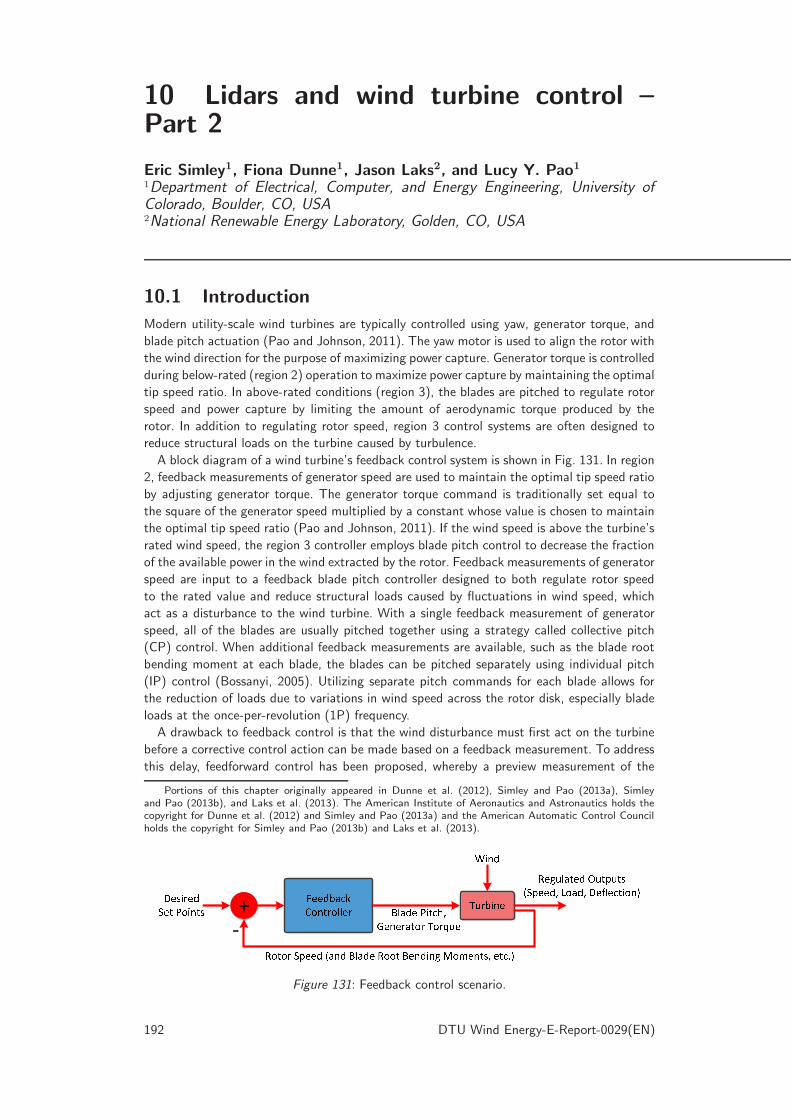
10 Lidars and wind turbine control –Part 2

Eric Simley1, Fiona Dunne1, Jason Laks2, and Lucy Y. Pao1

1Department of Electrical, Computer, and Energy Engineering, University ofColorado, Boulder, CO, USA2National Renewable Energy Laboratory, Golden, CO, USA

10.1 Introduction

Modern utility-scale wind turbines are typically controlled using yaw, generator torque, and

blade pitch actuation (Pao and Johnson, 2011). The yaw motor is used to align the rotor with

the wind direction for the purpose of maximizing power capture. Generator torque is controlled

during below-rated (region 2) operation to maximize power capture by maintaining the optimal

tip speed ratio. In above-rated conditions (region 3), the blades are pitched to regulate rotor

speed and power capture by limiting the amount of aerodynamic torque produced by the

rotor. In addition to regulating rotor speed, region 3 control systems are often designed to

reduce structural loads on the turbine caused by turbulence.

A block diagram of a wind turbine’s feedback control system is shown in Fig. 131. In region

2, feedback measurements of generator speed are used to maintain the optimal tip speed ratio

by adjusting generator torque. The generator torque command is traditionally set equal to

the square of the generator speed multiplied by a constant whose value is chosen to maintain

the optimal tip speed ratio (Pao and Johnson, 2011). If the wind speed is above the turbine’s

rated wind speed, the region 3 controller employs blade pitch control to decrease the fraction

of the available power in the wind extracted by the rotor. Feedback measurements of generator

speed are input to a feedback blade pitch controller designed to both regulate rotor speed

to the rated value and reduce structural loads caused by fluctuations in wind speed, which

act as a disturbance to the wind turbine. With a single feedback measurement of generator

speed, all of the blades are usually pitched together using a strategy called collective pitch

(CP) control. When additional feedback measurements are available, such as the blade root

bending moment at each blade, the blades can be pitched separately using individual pitch

(IP) control (Bossanyi, 2005). Utilizing separate pitch commands for each blade allows for

the reduction of loads due to variations in wind speed across the rotor disk, especially blade

loads at the once-per-revolution (1P) frequency.

A drawback to feedback control is that the wind disturbance must first act on the turbine

before a corrective control action can be made based on a feedback measurement. To address

this delay, feedforward control has been proposed, whereby a preview measurement of the

Portions of this chapter originally appeared in Dunne et al. (2012), Simley and Pao (2013a), Simleyand Pao (2013b), and Laks et al. (2013). The American Institute of Aeronautics and Astronautics holds thecopyright for Dunne et al. (2012) and Simley and Pao (2013a) and the American Automatic Control Councilholds the copyright for Simley and Pao (2013b) and Laks et al. (2013). !" #

$Figure 131: Feedback control scenario.

192 DTU Wind Energy-E-Report-0029(EN)

!"#$% &'( #

( )

*+,-./0120013+456416/1 2001-678*+/94+::04 ;<4-./0 =0><:6901 ?<9@<9ABC@001D E+61D F03:079 .+/GF0A.401C09 H+./9A I:610 H.97JDK0/0469+4;+4L<0F0:6MB1NOGP./1

=+9+4 C@001 B6/1 I:610 =++9 I0/1./> Q+,0/9AD 097RG

Figure 132: Combined feedback and feedforward control scenarios with (a) perfect preview

measurements and (b) lidar measurements and the effects of wind evolution.

wind disturbance is used directly as an input to the controller (see Fig. 132a). Original work

in feedforward control focused on regulating power capture in fluctuating wind conditions

using preview measurements provided by an upstream meteorological tower (Kodama et al.,

1999). Later, research concentrated on using lidar to remotely sense the wind speeds from

the turbine nacelle (Harris et al., 2005).

Lidar-based control has been investigated for use in both below-rated and above-rated

conditions. In below-rated region 2 control, turbine-mounted lidar measurements have been

proposed for correcting yaw error (Schlipf et al. 2011; Kragh et al. 2013) and increasing

power capture (Schlipf et al. 2011; Wang et al. 2012a; Bossanyi et al. 2012b). Through

simulation, it was found that a scanning lidar system can effectively estimate yaw error and

fine-tune the yaw alignment of a turbine as long as the inflow is not too complex (Kragh

et al., 2013). Lidar-assisted feedforward control in below-rated conditions has been shown

to provide a small increase in power capture (0.1 − 2%). However, the additional structural

loads caused by aggressively tracking the optimal tip speed ratio usually outweigh the power

capture improvement (Schlipf et al. 2011; Bossanyi et al. 2012b).

Recently, much of the lidar-based feedforward control research has focused on regulating

rotor speed and mitigating structural loads in above-rated conditions, where potential for

significant load reduction has been shown. As with feedback control, lidar-assisted control

in region 3 can be classified as either collective pitch or individual pitch control. Collective

pitch feedforward control strategies use the lidar measurements to estimate the effective

wind speed that the entire rotor will experience to regulate rotor speed and reduce tower

and collective blade loads (Wang et al. 2012b; Schlipf et al. 2012b; Bossanyi et al. 2012b).

Individual blade pitch control, however, allows for reduction of the loads experienced by

each separate blade, which could also be transferred to non-rotating components on the

DTU Wind Energy-E-Report-0029(EN) 193

turbine (Bir, 2008). Information from lidar measurements must be used to estimate the wind

speeds encountered by each individual blade. One class of controller designs uses information

from lidar measurements to estimate the hub-height, horizontal shear, and vertical shear

components of the wind, which are in turn used as inputs to the controller (Schlipf et al.

2010; Laks et al. 2011b; Bossanyi et al. 2012b). The other class of controllers uses a separate

measurement of the expected wind speed for each individual blade (Dunne et al. 2011b; Laks

et al. 2011b; Dunne et al. 2012). During the summer of 2012, a simple lidar-based collective

pitch feedforward controller designed to regulate rotor speed was tested at the US National

Renewable Energy Laboratory (NREL) with promising results (Scholbrock et al., 2013).

The simulation of lidar-based controllers is progressing toward more realistic preview mea-

surement modeling. Preliminary research included the assumption that upstream wind speeds

could be measured perfectly (Schlipf and Kuhn 2008; Dunne et al. 2011b; Laks et al. 2011b).

An additional assumption was that the measured wind speeds would reach the turbine un-

changed after a delay time of d/U , where d is the preview distance and U is the mean wind

speed (see Fig. 132a). The next generation of feedforward control simulations contained realis-

tic lidar models including spatial averaging of the wind speeds along the lidar beam (discussed

in Section 10.5.1) (Schlipf et al. 2009; Dunne et al. 2011a; Laks et al. 2011a; Simley et al.

2013c; Kragh et al. 2013). Recently, control simulations have included models of the impor-

tant source of error commonly referred to as “wind evolution” (discussed in Section 10.5.3)

(Bossanyi 2012; Laks et al. 2013). Wind evolution describes how the wind speeds change, or

evolve, as they travel downstream toward the turbine. The more realistic lidar measurement

scenario including wind evolution is shown in Fig. 132b. An additional source of measurement

error that has recently been included in simulation is uncertainty in the time it takes for the

measured wind to reach the rotor (Mirzaei et al., 2013).

10.1.1 Lidar Measurement Strategies

Several lidar technologies suitable for wind turbine control have been field tested in the past

decade. Harris et al. (2007) performed the first turbine-mounted lidar test using a continuous-

wave (CW) lidar (see Section 10.5.1) mounted on top of the nacelle. This lidar was simply

configured to stare straight ahead into the wind and focus at a particular distance. Rettenmeier

et al. (2010) employ a customized pulsed lidar system (see Section 10.5.1) that is also mounted

on top of the nacelle. The pulsed lidar provides measurements at a number of points along

the beam and can be aimed in any direction in front of the rotor using a mirror with two axes

of motion. Mikkelsen et al. (2013) have developed a circularly scanning CW lidar that can

be mounted in the hub, or spinner, of a turbine (see Fig. 133). This configuration allows for

continuous measurements without periodic blockage from passing blades. Recently, Pedersen

et al. (2013) have tested a CW lidar mounted directly on a turbine blade, allowing for direct

measurement of the wind speed and angle-of-attack that a rotating blade will experience.

The lidar measurement analyses in the rest of this chapter assume a circularly scanning

spinner-mounted lidar similar to the system developed by Mikkelsen et al. (2013). Figure 133

contains an illustration of the measurement scenario. The hub-mounted lidar measures a circle

of wind with scan radius r at a preview distance d upstream of the rotor. Although it is possible

to scan faster than the rotational speed of the rotor (Mikkelsen et al., 2013), the analyses

in this chapter assume that the lidar spins with the rotor, allowing the lidar to measure the

wind that a single blade will experience. The relative simplicity of this measurement scenario

allows for careful analysis of measurement performance. Unless otherwise specified, the lidar

investigations in this chapter are performed using the NREL 5-MW reference turbine model

(Jonkman et al., 2009) which has a hub height of 90 m and a rotor radius of 63 m.

The remainder of this chapter is organized as follows. Section 10.2 presents the region

3 feedforward control scenario using a linear wind turbine model. The feedforward control

strategy that minimizes the variance of an output error variable such as generator speed or

a structural load is derived for the case of imperfect lidar measurements. An explanation

of why measurement preview is required in feedforward wind turbine control is presented in


-100-50

0-50

0

50

0

50

100

150

horizontal (m)along wind (m)

vert

ical (m

)d

r

R

w

u

v

Figure 133: Measurement scenario for the 5-MW reference turbine. The variable d represents

the preview distance upwind of the turbine where measurements are taken. r represents the

radius of the scan circle and R indicates the 63 m rotor radius. The dots represent where

measurements are taken for the circularly scanning lidar and the magenta curve illustrates the

range weighting function along the lidar beam (see Section 10.5.1).

Section 10.3. Section 10.4 describes the wind speed quantity of interest for blade pitch control,

referred to as “blade effective wind speed.” Section 10.5 describes how measurements from

a hub-mounted lidar can be used to estimate blade effective wind speed. The main sources

of lidar measurement error are discussed here as well. The topics in Sections 10.2, 10.4,

and 10.5 are combined to illustrate a lidar measurement design scenario in Section 10.6,

with the objective of minimizing the mean square value of blade root bending moment using

feedforward control. Examples of lidar-based feedforward controller designs using simulation

are included in Sections 10.7 and 10.8. Finally, Section 10.9 summarizes the material presented

in the chapter.

10.2 Wind Turbine Feedforward Control

The combined feedback/feedforward control scenario for above-rated conditions used in this

chapter is described in Fig. 134. A blade pitch control loop using feedback from rotor speed

regulates an output variable y (such as generator speed error or a structural load), which

represents the deviation from a set point. Generator torque is controlled to be inversely

proportional to generator speed to maintain the rated 5 MW of power (Jonkman et al., 2009).

The feedback control loop is designed for the mean wind speed U such that any wind speed

deviation acts as a disturbance wt on the turbine. The feedback control loop is augmented with

a blade pitch feedforward controller F which uses the preview wind disturbance measurement

wm, provided by a lidar. Additionally, a prefilter Hpre can be introduced between the lidar

measurement and the feedforward controller to provide an estimate wt of the wind disturbance

based on wm. The original upstream wind worig is measured by the lidar yielding the distorted

measurement wm. As worig travels downstream toward the turbine, it will undergo distortion

due to wind evolution until it interacts with the turbine as wt after a delay of d/U .

10.2.1 Feedforward Control Assuming Perfect Measurements

When feedforward is not used (F = 0), the output variable y is given by

y = Tywtwt (214)


+

F

PC

FF

LidarHpre

Evo.

worig

wt

wm

y

FB

t

T

gen yFB

Figure 134: Block diagram of the feedforward control scenario. P is the linearized turbine

model and C is the feedback controller, controlling blade pitch and generator torque deviations

from the operating point using a measurement of generator speed error yFB. T represents the

turbine with feedback control, as enclosed in the dashed box. y is the output error variable of

interest, which is intended to be regulated to 0. F represents the ideal feedforward controller

(assuming perfect measurements) and Hpre is the prefilter used to estimate a preview of the

wind disturbance wt based on the lidar measurement wm. worig is the original upstream wind

speed which becomes wm after lidar measurement and wt after experiencing wind evolution

and arriving at the turbine.

where Tywtis the transfer function from the wind disturbance wt to y. With the introduction

of feedforward control without a prefilter (Hpre = 1), y becomes a function of both wt and

wm:

y = Tywtwt + TyβFF

Fwm (215)

where TyβFFis the transfer function from the feedforward blade pitch command βFF to

y. When measurements are perfect (wm = wt) and there is perfect turbine modeling, the

feedforward controller that completely cancels the effect of the disturbance wt on the turbine

is given by

F = −T−1yβFF

Tywt, (216)

which yields the output y = 0 in Eq. (215). In reality, non-minimum phase (unstable) zeros

in TyβFFcan cause the ideal F to be unstable (Dunne et al., 2011b). In this case, a stable

approximation to the ideal F is used (Dunne et al., 2011b). For the analysis in this chapter,

however, it is simply assumed that F = −T−1yβFF

Tywt. When the measurements are not perfect

(wm 6= wt), the output is

y = Tywt(wt − wm) . (217)

Due to the distorting effects of the lidar and wind evolution along with the spatial averaging

of the wind caused by the area of the turbine rotor, in general wm 6= wt. In this case, the

variance, or mean square magnitude, of y in the frequency domain is given by

|Y (f)|2 = |Tywt(f)|2 |Wt(f)−Wm(f)|2

= |Tywt(f)|2 (Swtwt

(f) + Swmwm(f)− 2ℜSwtwm

(f))(218)

where Swtwt(f) represents the power spectral density (PSD) of the wind disturbance, Swmwm

(f)

is the PSD of the lidar measurement, Swtwm(f) is the cross-power spectral density (CPSD)

between the wind disturbance and the lidar measurement, and ℜ indicates the real part of

a complex value. The variance of y in the time domain is calculated by integrating Eq. (218)

over all frequencies:

Var (y) =

∫ ∞

−∞

|Tywt(f)|2 (Swtwt

(f) + Swmwm(f)− 2ℜSwtwm

(f)) df. (219)


With feedback only, on the other hand, the variance of y is simply

|Y (f)|2 = |Tywt(f)|2 Swtwt

(f) (220)

in the frequency domain and

Var (y) =

∫ ∞

−∞

|Tywt(f)|2 Swtwt

(f)df (221)

in the time domain. Section 10.2.3 provides an explanation for treating reduction in variance

as a control objective.

By comparing Eq. (218) with Eq. (220), the frequencies where feedforward control with

wt = wm is beneficial can be found. Ideal feedforward control with no prefilter reduces the

variance of y at the frequencies where Eq. (222) is satisfied:

Swtwt(f) + Swmwm

(f)− 2ℜSwtwm(f) < Swtwt

(f) . (222)

Equation (222) can be rearranged as

1

2<

ℜSwtwm(f)

Swmwm(f)

. (223)

10.2.2 Feedforward Control with Imperfect Measurements

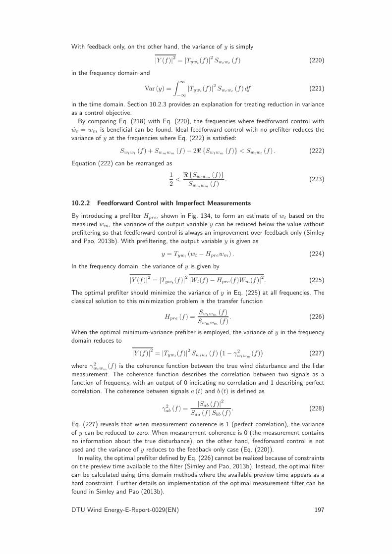
By introducing a prefilter Hpre, shown in Fig. 134, to form an estimate of wt based on the

measured wm, the variance of the output variable y can be reduced below the value without

prefiltering so that feedforward control is always an improvement over feedback only (Simley

and Pao, 2013b). With prefiltering, the output variable y is given as

y = Tywt(wt −Hprewm) . (224)

In the frequency domain, the variance of y is given by

|Y (f)|2 = |Tywt(f)|2 |Wt(f)−Hpre(f)Wm(f)|2. (225)

The optimal prefilter should minimize the variance of y in Eq. (225) at all frequencies. The

classical solution to this minimization problem is the transfer function

Hpre (f) =Swtwm

(f)

Swmwm(f)

. (226)

When the optimal minimum-variance prefilter is employed, the variance of y in the frequency

domain reduces to

|Y (f)|2 = |Tywt(f)|2 Swtwt

(f)(1− γ2wtwm

(f))

(227)

where γ2wtwm(f) is the coherence function between the true wind disturbance and the lidar

measurement. The coherence function describes the correlation between two signals as a

function of frequency, with an output of 0 indicating no correlation and 1 describing perfect

correlation. The coherence between signals a (t) and b (t) is defined as

γ2ab (f) =|Sab (f)|2

Saa (f)Sbb (f). (228)

Eq. (227) reveals that when measurement coherence is 1 (perfect correlation), the variance

of y can be reduced to zero. When measurement coherence is 0 (the measurement contains

no information about the true disturbance), on the other hand, feedforward control is not

used and the variance of y reduces to the feedback only case (Eq. (220)).

In reality, the optimal prefilter defined by Eq. (226) cannot be realized because of constraints

on the preview time available to the filter (Simley and Pao, 2013b). Instead, the optimal filter

can be calculated using time domain methods where the available preview time appears as a

hard constraint. Further details on implementation of the optimal measurement filter can be

found in Simley and Pao (2013b).


0 200 400 600 800 10000

500

1000

1500

2000

2500

3000

3500

4000

RootMyb1 standard deviation (kNm)

Ro

otM

yb

1 D

EL

(kN

m)

m=10

m=3

Figure 135: DEL vs STD values of blade root flapwise bending moment (RootMyb1) from

various simulations of the NREL 5-MW wind turbine. The DEL calculation depends on m,

the slope of the S-N (stress vs. cycles to failure) curve for the particular material. The value

m=3 is typical for welded steel, and m=10 is typical for composite blades.

10.2.3 The Relationship between Variance and Damage Equivalent Loads

Aside from regulating generator speed, the objective of the control in above-rated conditions is

to minimize variations in stress on turbine components because they cause material fatigue,

which over time leads to failure. The damage equivalent load (DEL) (IEC, 2001) is the

standard method of quantifying fatigue damage. However, the DEL is a fairly complicated

nonlinear function of a load on a turbine component, and it is difficult to minimize directly.

Instead, the standard deviation (STD) of a load can be minimized, and this is correlated with

reduction in the DEL, as shown in Fig. 135. Minimizing variance is the same as minimizing

standard deviation because the variance is simply the standard deviation squared.

10.3 Preview Time in Feedforward Control

10.3.1 Ideal Feedforward Controller Preview Time

The ideal feedforward controller (Eq. (216)) is typically non-causal, and therefore not imple-

mentable except by causal approximation or by using a preview measurement of the wind. This

non-causality appears whenever TyβFFhas more phase delay than Tywt

, or in other words,

the blade pitch command takes longer to affect the output of interest than does the wind

disturbance. This happens whenever a blade pitch actuator model is included, and it has also

been observed when blade-flexibility is modeled. The difference in phase delay between TyβFF

and Tywtdetermines how much preview time is required to implement the ideal controller. A

smaller-than-ideal amount of preview time is still useful, allowing a better approximation to

the ideal controller than would be possible with no preview time at all.

The pitch actuator for the NREL 5-MW wind turbine is typically modeled as a 2nd-order

low-pass filter with a natural frequency of 1 Hz and a damping ratio of 0.7. This results in a

delay of about 0.225 seconds that appears in TyβFFbut not Tywt

. Phase delay is converted

to time delay using the equation

time delay = −phase/360/frequency.

The time delay is a function of frequency, but remains fairly constant at low frequencies, and

we use this low-frequency value of the time delay.

When blade flexibility is modeled on the NREL 5-MW wind turbine, and when the output

y is chosen to be generator speed error, the delay in TyβFFfurther increases relative to Tywt

.


12 14 16 18 20 22 24

1.5

2

2.5

3

wind speed (m/s)

required p

revie

w t

ime f

or

LP

F (

s)

Figure 136: Estimated preview required to cancel the delay of the prefilter, as a function of

wind speed. The prefilter is assumed to be a 2nd order low-pass Butterworth filter with cutoff

frequency corresponding to 0.04 rad/m.

The physical reason for this blade-flexibility delay is not understood, but it does conincide

with non-minimum phase zeros in the linearized turbine model. The resulting delay ranges

from 0.05 to 0.3 seconds depending on average wind speed. Additional or different delay in

TyβFFrelative to Tywt

may appear when a different output of interest is chosen.

10.3.2 Prefilter Preview Time

In addition to the preview time required to implement the ideal feedforward controller, preview

time is needed to implement the minimummean square error prefilter (Eq. (226)). The prefilter

generally takes the form of a low-pass filter, where the better the wind measurements are,

the higher the cutoff frequency of the low-pass filter is. Every low-pass filter introduces delay

(or requires equivalent advance knowledge of the incoming signal). The higher the cutoff

frequency of the low-pass filter, the less delay is introduced at any given frequency. Therefore

better measurements mean less delay introduced in the prefilter and less required preview

time.

A typical nacelle-mounted lidar, designed for control, yields good measurements up to a

wavenumber of about 0.04 rad/m. For a wind speed of 13 m/s for example, this frequency is

0.04 rad/m× 13 m/s/(2π rad) ≈ 0.08 Hz.

Figure 136 shows the preview time required (the time delay introduced at low frequencies)

by the prefilter, assuming it is a 2nd-order low-pass Butterworth filter with a cutoff frequency

corresponding to 0.04 rad/m. (The amount of delay introduced depends on the order of the

filter in addition to the cutoff frequency. A higher-order means a steeper cutoff and more

delay introduced.) We see that the preview time needed for the prefilter is much greater

than the preview time needed for the ideal feedforward controller, and it decreases with

increasing wind speed, ranging from about 1.5 to 3 seconds. Preview time available from

the lidar measurement also decreases with increasing wind speed because it is determined by

the preview distance divided by the average wind speed. More detail on required preview time

due to pitch actuators, blade flexibility, and imperfect wind measurements can be found in

Dunne et al. (2012).

10.3.3 Pitch Actuation Preview Time

The ideal model-inverse feedforward controller design method assumes we want to minimize a

single output or set of outputs, such as generator speed error or blade root bending moments,


with no restriction on pitch actuation. However, we may want to minimize pitch actuation in

addition to generator speed error or particular loads of interest. It is possible that additional

preview time may be useful in meeting this combined objective. This topic is currently under

investigation.

10.4 Blade Effective Wind Speed

Before analyzing lidar measurement error in depth, it is important to define the wind speed

quantities that are of interest for blade pitch control. For collective pitch control, the effective

wind speed experienced by the rotor is often calculated by integrating the wind speeds across

the entire rotor disk using the formula:

urotor =

∫ 2π

0

∫ R

0

u3 (r, φ)CP (r) rdrdφ

∫ 2π

0

∫ R

0

CP (r) rdrdφ

1

3

, (229)

where CP (r) is the radially-dependent coefficient of power and R is the rotor radius (Schlipf

et al., 2012b). The resulting urotor is the uniform wind speed that would produce the same

power as the actual distribution of wind speeds across the rotor disk. Note that Eq. (229) is

only a function of the u component of wind, which is perpendicular to the rotor plane (see

Fig. 133), rather than also including the horizontal v and vertical w components. Because u

has a significantly greater impact on the turbine’s aerodynamics than v or w, the calculation

of effective wind speeds at the turbine is performed solely for the u component. Section 10.4.1

describes the relative importance of the u, v, and w wind speed components in further detail.

For individual pitch control, the effective wind speeds experienced by each individual blade

are of interest, rather than a rotor averaged quantity. The blade effective wind speed used here

is a weighted sum of wind speeds along the blade span such that wind speeds at each location

are weighted according to their contribution to overall aerodynamic torque. Aerodynamic

torque δQ (r) produced by a segment of the blade with spanwise thickness δr at radial

distance r along the blade can be described using the radially dependent coefficient of torque

CQ (r) as

δQ (r) = ρπr2u2 (r)CQ (r) δr, (230)

where ρ is the air density and u (r) is the u component of the wind speed at radial distance

r along the blade (Moriarty and Hansen 2005; WT Perf 2012). Although other weighting

variables could be chosen for the definition of blade effective wind speed, aerodynamic torque

is used here because it is directly related to the power generated by the turbine.

Using Eq. (230), the torque-based blade effective wind speed is given by

ublade =

∫ R

0

u2 (r)CQ (r) r2dr

∫ R

0

CQ (r) r2dr

1

2

. (231)

A linearized form of Eq. (231) is used to calculate blade effective wind speed by integrating

the wind speeds along the blade using the linear weighting function

Wb (r) =CQ (r) r2

∫ R

0

CQ (r) r2dr

. (232)

A linear blade effective wind speed is used because of its simplicity and because the statistics

of a linear combination of wind speeds are generally easy to calculate. Figure 137 illustrates

the blade effective weighting function Wb (r) calculated using WT Perf (2012) for the NREL

5-MW turbine model at the rated wind speed U = 11.4 m/s, and two above-rated wind

speeds (13 m/s and 15 m/s). In above-rated conditions, the weighting curves change with

wind speed because the steady-state blade pitch angle increases as wind speed increases

(Jonkman et al., 2009).


0 6.3 12.6 18.9 25.2 31.5 37.8 44.1 50.4 56.7 63

Spanwise Position, r (m)

Norm

aliz

ed

CPr

= C

Qr2

0 10 20 30 40 50 60 70 80 90 100

0

0.2

0.4

0.6

0.8

1U = 11.4 m/s

U = 13 m/s

U = 15 m/s

40 50 60Blade Span (%)

Wb(r

)

Figure 137: Aerodynamic torque-based blade effective weighting functionWb (r) for the NREL

5-MW turbine model at the rated wind speed 11.4 m/s and two above-rated wind speeds.

10.4.1 The Relative Importance of the u, v, and w Components

When a turbine is operating in above-rated wind speeds, variations in the u component of

the wind have a much greater effect than variations in the v and w components, in terms of

their effect on generator speed and structural loads. To illustrate this point, linearized transfer

functions from wind speed to variables of interest were generated for the 5-MW model using

NREL’s FAST software (Jonkman and Buhl, 2005). For example, in Fig. 138, which shows the

magnitude frequency responses of several transfer functions, the effect of the u component

is generally about ten times (20 dB) greater than that of the v and w components, when

looking at the frequencies where the turbine speed and loads are most affected. There are

some frequencies at which v and w have a greater effect than u on the vertical and horizontal

components of blade root bending. However, all wind inputs shown are uniform over the

rotor plane, and shear was not included. It is expected that the magnitude of the transfer

functions from vertical and horizontal shear in the u component of the wind to the vertical

and horizontal components of blade root bending would be much higher than the magnitude

of the transfer functions from the v and w components.

The u component likely has a greater effect than v and w in part because the turbine

blades move quickly in the direction of the v and w components. In above-rated wind speeds,

a turbine’s tip speed is typically around 70 m/s, so the outboard half of the blade (which is

most influential in power capture and loads) is moving through the v and w wind components

at 35 to 70 m/s. The angle of attack seen by a blade section is more influenced by a small

change in the 13 m/s u component than a small change in the 35 to 70 m/s v or w component

it sees.

10.5 Lidar Measurements

The performance of lidar measurements is investigated using the hub-mounted, circularly

scanning lidar scenario shown in Fig. 133. The lidar model is based on the ZephIR 300

continuous-wave lidar (Slinger and Harris, 2012), which has a sampling rate of 50 Hz. Mea-

surement performance is assessed as a function of the two scan parameters: scan radius r and

preview distance d.

In general, measurement quality is described using the coherence between the lidar mea-

surement and the blade effective wind speed. The coherence calculations require a frequency


100

50

0

50

To:

GenS

peed

50

0

50

100

To:

RootM

ycC

50

0

50

To:

RootM

ycV

103

102

101

100

101

50

0

50

To:

RootM

ycH

Bode Diagram

Frequency (Hz)

Magnitude (

dB

)

From: u

From: v

From: w

Figure 138: Plots of the magnitude frequency response of the closed-loop transfer functions

from the u, v, and w components of wind speed (m/s) to (from upper to lower plots)

generator speed error (rpm) and the collective, vertical, and horizontal components of blade

root bending moment (kN·m) for the NREL 5-MW turbine, with all 16 degrees of freedom,

linearized at 13 m/s.

domain model of the wind field. The wind field used here is based on the IEC von Karman

isotropic model for neutral atmospheric stability (Jonkman, 2009). An above-rated mean wind

speed U = 13 m/s is used, along with a turbulence intensity of 10%. Wind speeds are spa-

tially correlated in the transverse y and vertical z directions using the IEC coherence formula

(Jonkman 2009; IEC 2005). Whereas the IEC standard only defines spatial coherence for the

u component of wind speed, we apply the coherence formula to the spatial correlation of the

v and w components as well.

Lidar measurements and blade effective wind speeds are calculated as weighted sums of

wind speeds along the lidar beam and blade span. Conveniently, the spectra of weighted

sums of wind speeds are easy to calculate. For example, the CPSD between signals a (t) =M∑

m=0

αmam (t) (A(f) in the frequency domain) and b (t) =

N∑

n=0

βnbn (t) (B(f) in the fre-

quency domain), which are linear combinations of other signals, can be calculated as

Sab (f) = A (f)B∗ (f)

=

(M∑

m=0

αmAm (f)

)(N∑

n=0

β∗nB

∗n (f)

)

=

M∑

m=0

N∑

n=0

αmβ∗nSambn (f),

(233)

as long as the CPSDs Sambn (f) are known for each m and n. The symbol ∗ represents the

complex conjugate operator. The wind field model used here defines the CPSDs between wind

speeds at any two locations, allowing the spectra of lidar measurements and blade effective

wind speeds to be calculated.


10-3

10-2

10-1

100

0

0.2

0.4

0.6

0.8

1

Frequency (Hz)

Co

he

ren

ce

Point to Blade Effective Wind Speed Coherence

r = 25% R

r = 50% R

r = 70% R

r = 84% R

r = 100% R

0 6.3 12.6 18.9 25.2 31.5 37.8 44.1 50.4 56.7 63

Spanwise Position, r (m)

No

rma

lize

d C

Pr

= C

Qr2

0 10 20 30 40 50 60 70 80 90 100

0

0.2

0.4

0.6

0.8

1 Weighting, U = 11.4 m/s

r = 25% R

r = 50% R

r = 70% R

r = 84% R

r = 100% R

Wb(r

)

40 50 60Blade Span (%)

Figure 139: Coherence between the wind speeds at single points along the blade and overall

blade effective wind speed for the NREL 5-MW model at U = 11.4 m/s.

The scan radius r of the circularly scanning lidar should be chosen to produce high measure-

ment coherence between the measured wind and the blade effective wind speed. Figure 139

shows the coherence between perfectly measured u wind speeds at various points along the

blade and blade effective wind speed. Coherence is highest for wind speed measurements near

the outboard region of the blade, where torque production is highest. Note that low-frequency

coherence happens to be maximized when the wind is measured at 70% blade span rather

than at 84% span, where the peak of the weighting function is located, due to the partic-

ular spatial coherence model used. For control purposes, it is more important to maximize

coherence at low frequencies, where the power in the turbulence spectrum is concentrated.

10.5.1 Range Weighting

As illustrated by the magenta curve on the lidar beam in Fig. 133, a CW lidar measures

weighted line-of-sight wind speeds along the entire beam, where the peak of the weighting

function is located at the intended focus point. A weighted line-of-sight lidar measurement

can be described as

uwt,los = −ℓxuwt − ℓyvwt − ℓzwwt (234)

where ℓ = [ℓx, ℓy, ℓz] is the unit vector in the direction that the lidar is pointing. uwt,

vwt, and wwt are the weighted velocities along the lidar beam such that the vector ~uwt =

[uwt, vwt, wwt] is given by

~uwt =

∫ ∞

0

~u(Rℓ~ℓ+ [0, 0, h]

)W (Fℓ, Rℓ)dRℓ (235)


0 50 100 150 200 250 3000

0.2

0.4

0.6

0.8

1

Range Rl (m)

No

rma

lize

dW

(Fl ,

Rl )

Fl = 50 m F

l = 125 m F

l = 200 m Pulsed

Figure 140: Normalized range weighting function W (Fℓ, Rℓ) for a CW lidar similar to the

ZephIR 300 at three different focus distances along with the range weighting function for a

pulsed lidar similar to the Windcube WLS7.

where the velocity vector ~u = [u, v, w] is defined such that the u velocity is in the x direction,

v is in the y direction, and w is in the z direction (see Fig. 133). Hub height is represented

by h. The minus signs appear in Eq. (234) because the measured line-of-sight velocity is the

projection of the velocity vector onto the direction from the measurement point to the lidar,

opposite from the lidar look direction. W (Fℓ, Rℓ) is the range weighting function with focus

distance Fℓ and range along the lidar beam Rℓ as arguments.

The range weighting function for a CW lidar becomes broader as the focus distance in-

creases (the Full width at half maximum of W (Fℓ, Rℓ) scales with the square of the focus

distance Fℓ) (Frehlich and Kavaya 1991; Slinger and Harris 2012). W (Fℓ, Rℓ) is plotted as

a function of range along the lidar beam for three different focus distances in Fig. 140. Also

included in Fig. 140 is the range weighting function for a pulsed lidar similar to the Windcube

WLS7 (Frehlich et al. 2006; Mikkelsen 2009). Note that the pulsed lidar range weighting

function does not vary with measurement distance. Additional details on CW and pulsed

range weighting functions can be found in Simley et al. (2013c).

10.5.2 Geometry Errors

As mentioned in Section 10.4.1, the u component of the wind speed is of interest for wind

turbine control. An estimate of the u component is formed by dividing the line-of-sight

measurement in Eq. (234) by −ℓx, yielding

u = − 1ℓxuwt,los

= uwt +ℓyℓxvwt +

ℓzℓxwwt.

(236)

As revealed in Eq. (236), detection of the v and w wind speed components causes a degrada-

tion in the estimate of the u component. For a fixed scan radius r, short preview distances d

will result in large measurement angles, causing significant measurement error due to detec-

tion of the v and w components (Simley et al., 2013c). As preview distance increases, theℓyℓx

and ℓzℓx

terms decrease and error caused by measurement geometry will decrease. Figure 141

contains coherence curves for a hub-mounted lidar without range weighting measuring at a

scan radius of r = 41 m for different preview distances. The coherence curves represent the

correlation between the lidar measurement and the wind speed at a single point downstream

of the measurement, so that only geometry errors are included. As preview distance increases,

the measurement coherence increases due to less contribution from the v and w components

in Eq. (236).


10−3

10−2

10−1

100

0

0.2

0.4

0.6

0.8

1

Frequency (Hz)

Cohere

nce

Geometry Errors, r = 41 m

d = 30 m

d = 60 m

d = 90 m

d = 120 m

d = 150 m

Figure 141: Measurement coherence for a hub-mounted lidar with a scan radius of 41 m at

five different preview distances. Only geometry errors are included.

10−3

10−2

10−1

100

0

0.2

0.4

0.6

0.8

1

Frequency (Hz)

Co

he

ren

ce

Wind Evolution, r = 41 m

d = 30 m

d = 60 m

d = 90 m

d = 120 m

d = 150 m

Figure 142: Measurement coherence for a hub-mounted lidar with a scan radius of 41 m at

five different preview distances. Only wind evolution errors are included.

10.5.3 Wind Evolution

A major source of preview measurement error is the evolution of the turbulence between

the time it is measured by the lidar and the time it appears at the turbine rotor as a wind

disturbance. While for a fixed scan radius r, measurement errors due to the measurement

geometry decrease as preview distance increases, errors due to wind evolution become more

severe, since there is additional time for the turbulence to evolve.

Wind evolution can be described by a coherence function between wind speeds at two

points separated in the longitudinal (along-wind) direction. A popular longitudinal coherence

formula used in the wind turbine control community (Bossanyi et al. 2012b; Schlipf et al.

2012a; Laks et al. 2013) is presented in Kristensen (1979). The Kristensen coherence formula

is a function of frequency, longitudinal separation, mean wind speed, turbulent kinetic energy,

and a turbulence length scale. Wind evolution becomes more severe when longitudinal sepa-

ration or turbulent kinetic energy are increased and becomes less severe as mean wind speed

increases. Longitudinal coherence curves using the Kristensen (1979) formula are shown in

Fig. 142 for several preview distances. A mean wind speed of 13 m/s is used with a turbulence

intensity of 10%. Wind evolution tends to affect high frequencies more than low frequencies

and, as a result, very low-frequency structures in the wind do not change significantly between

the measurement point and the turbine.

The IEC von Karman wind model used in this chapter only defines spatial coherence in

the transverse and vertical (yz) plane. This model assumes that wind speeds are perfectly


10−3

10−2

10−1

100

0

0.2

0.4

0.6

0.8

1

Frequency (Hz)

Co

he

ren

ce

Estimation of Point Wind Speeds, r = 41 m

d = 30 m

d = 90 m

d = 150 m

d = 30 m, w/ Lidar

d = 90 m, w/ Lidar

d = 150 m, w/ Lidar

Figure 143: Coherence between lidar measurements and the wind speed at a point 41 m

along the blade for a hub-mounted lidar with a scan radius of 41 m for three different

preview distances. Geometry errors and wind evolution are included. The solid curves represent

measurement coherence without lidar range weighting while the dashed curves include range

weighting.

correlated in the x direction, i.e., wind speeds simply “march” downstream without evolving.

Wind evolution is added to this wind field model by introducing imperfect longitudinal spatial

coherence. We define spatial coherence for wind speeds at any two locations as the prod-

uct between the spatial coherence defined in Jonkman (2009) due to the separation in the

transverse (y) and vertical (z) directions and the longitudinal coherence due to separation in

the x direction. Additional details on the application of the Kristensen (1979) wind evolution

formula to wind field modeling can be found in Simley and Pao (2013a) and Laks et al.

(2013).

10.5.4 Lidar Measurements of Blade Effective Wind Speed

Figures 141 and 142 reveal measurement coherence including the effects of geometry errors

and wind evolution separately, where the variable of interest is the wind speed at a single point

41 m along the blade. Figure 143 contains measurement coherence curves for a fixed scan

radius of r = 41 m including the combined effects of geometry errors and wind evolution for

three different preview distances, with and without the effects of lidar range weighting. As pre-

view distance increases, low-frequency correlation improves, due to diminishing measurement

geometry effects, but high-frequency correlation becomes worse because of the additional

wind evolution. Since more power in the wind is located at lower frequencies, it is important

to have good low-frequency measurement correlation even if high-frequency correlation suf-

fers. Lidar range weighting causes an overall drop in measurement coherence with the wind

speed at a single point along the blade due to spatial averaging of the wind field.

As discussed earlier, blade effective wind speed is the wind speed quantity of interest for

blade pitch control purposes, rather than the wind speed at a single point along the blade. The

coherence between lidar measurements and blade effective wind speed for the same preview

distances that are included in Fig. 143 are shown in Fig. 144. Measurement coherence tends

to decrease compared to the results in Fig. 143 because of the spatial averaging of the wind

field caused by blade effective weighting. However, when the variable of interest is blade

effective wind speed, lidar range weighting actually improves measurement coherence. We

attribute this improvement to the spatial averaging of the lidar measurement “mimicking”

the spatial averaging of wind speeds along the blade. Further details on the calculation of lidar

measurement coherence for measurement scenarios including geometry errors, wind evolution,

and range weighting can be found in Simley et al. (2012).


10−3

10−2

10−1

100

0

0.2

0.4

0.6

0.8

1

Frequency (Hz)

Co

he

ren

ce

Estimation of Blade Effective Wind Speeds, r = 41 m

d = 30 m

d = 90 m

d = 150 m

d = 30 m, w/ Lidar

d = 90 m, w/ Lidar

d = 150 m, w/ Lidar

Figure 144: Coherence between lidar measurements and blade effective wind speed for a hub-

mounted lidar with a scan radius of 41 m for three different preview distances. Geometry

errors and wind evolution are included. The solid curves represent measurement coherence

without lidar range weighting while the dashed curves include range weighting.

10.6 Lidar Measurement Example: Hub Height and ShearComponents

In the previous section, the measurement quality between a lidar measurement and blade

effective wind speed at a fixed location was investigated. In reality, the blades of a turbine

rotate through the wind field and it is the total contribution from all blades comprising the

rotor that affects the turbine. For a three-bladed turbine, such as the NREL 5-MW model, the

wind speeds felt by the rotating blades can be described as the sum of a collective component,

which all three blades experience; a linear vertical shear component, which describes the

gradient of the wind speeds in the vertical z direction; and a linear horizontal shear component,

which describes the wind speed gradient in the horizontal y direction. These collective and

shear components describe the u component of wind speed in the rotor plane.

The three blade effective wind speeds, using the weighting function Wb (r) defined in

Eq. (232), can be written in terms of collective and shear components asublade,1ublade,2ublade,3

=

1 B cos (ψ) −B sin (ψ)

1 B cos(ψ + 2π

3

)−B sin

(ψ + 2π

3

)

1 B cos(ψ + 4π

3

)−B sin

(ψ + 4π

3

)

uhh∆v

∆h

(237)

where ψ is the azimuth angle in the rotor plane corresponding to blade number one, uhh is

the wind speed at hub height, ∆v is the difference in the wind speed across the rotor disk in

the vertical direction normalized by the mean wind speed U , ∆h is the difference in the wind

speed across the rotor in the horizontal direction normalized by the mean wind speed, and

B =U

2R

∫ R

0

Wb (r) rdr. (238)

Azimuth angle is defined such that ψ = 0 corresponds to the top of rotation (in the z

direction) and ψ = 90 corresponds to the left side of the rotor disk when facing upwind

(in the −y direction). By inverting Eq. (237), the collective and shear components can be

described as a function of the three blade effective wind speeds asuhh∆v

∆h

=

13

13

13

23B cos (ψ) 2

3B cos(ψ + 2π

3

)23B cos

(ψ + 4π

3

)

− 23B sin (ψ) − 2

3B sin(ψ + 2π

3

)− 2

3B sin(ψ + 4π

3

)

ublade,1ublade,2ublade,3

. (239)

Using the frequency domain description of the wind field with defined power spectra and

spatial coherence functions, the spectrum of the wind experienced by a blade rotating through

the wind field can be calculated, as explained in Simley and Pao (2013a). The method in


10−2

10−1

100

10−2

10−1

100

101

102

103

Frequency (Hz)

PS

D (

m2/s

)

Blade and Rotor Effective Wind Speed Spectra

Rotor Effective Wind Speed (Entire Disk)

Blade Effective Wind Speed

Collective Component, uhh

Shear components, ∆h, ∆

v

Figure 145: Power spectra of rotating blade effective wind speed as well as collective and

shear components due to three rotating blades. The rotor effective wind speed, calculated

by integrating wind speeds weighted according to their contribution to power over the entire

rotor disk, is shown for comparison. Spectra are generated for the IEC von Karman wind field

model using the NREL 5-MW turbine at mean wind speed 13 m/s.

Simley and Pao (2013a) can be extended to calculate the spectra of the collective and

shear components due to three rotating blades, using Eq. (239). Using the IEC von Karman

wind field and the NREL 5-MW model, the rotating blade effective wind speed and rotating

collective and shear terms are plotted in Fig. 145 for the rated rotor speed 12.1 rpm (0.202 Hz)

and above-rated wind speed 13 m/s. The blade effective wind speed spectrum contains peaks

at the 1P frequency (0.202 Hz) and its harmonics, due to the blade passing through turbulent

structures once per revolution. The collective and shear component spectra contain peaks at

the 3P (three times per revolution) frequency (0.606 Hz) and its harmonics because each of

the three blades passes through structures once per revolution. Also shown in Fig. 145 is the

rotor effective wind speed averaged across the entire rotor disk, calculated using Eq. (229),

to highlight the difference between modeling rotor effective wind speed as the wind felt by

the rotor disk and the wind felt by three rotating blades.

For wind turbine controls, it is popular to use linear models of the turbine in the non-rotating

frame because the resulting transfer functions do not vary with azimuth angle as much as

in the rotating frame. Rotating variables at each of the three blades are instead represented

as a collective component y0, a vertical component yv, and a horizontal component yh. For

example, the flapwise bending moment experienced by each blade can be represented as the

average bending moment over all blades (y0), the net bending moment of the rotor around the

y axis (yv), and the net bending moment around the vertical z axis (yh). Transfer functions

are calculated in the non-rotating frame using the multiblade coordinate (MBC) transform

(Bir, 2008), which is used as the basis for Eqs. (237) and (239). The response of the collective

component of a turbine variable is dominated by the collective wind component uhh, and the

vertical and horizontal components are dominated by the vertical ∆v and horizontal ∆h shear

components of the wind, respectively. Figure 146 contains the magnitude squared frequency

response of the transfer functions from hub height wind speed to the collective component of

flapwise blade root bending moment as well as the transfer functions from horizontal shear

and vertical shear to the horizontal component and vertical component of blade root bending

moment generated using FAST (Jonkman and Buhl, 2005) with the 5-MW model at the

above-rated wind speed 13 m/s. These transfer functions include blade pitch and generator


10−2

10−1

100

104

105

106

107

108

Frequency (Hz)

Magnitude S

quare

d

Wind to Blade Root Bending Moment

|Hy

0,u

hh

|2

|Hy

v,∆

v

|2

|Hy

h,∆

h

|2

Figure 146: Transfer functions from hub height wind speed uhh to the collective component

of flapwise blade root bending moment y0 as well as the transfer functions from vertical

shear ∆v and horizontal shear ∆h to the vertical component yv and horizontal component

yh of blade root bending moment. The transfer functions correspond to the NREL 5-MW

turbine model at above-rated wind speed 13 m/s including feedback control of blade pitch

and generator torque.

torque feedback control (Jonkman et al., 2009) using rotor speed measurements.

A lidar measurement scenario is proposed that uses three rotating measurements to estimate

the three rotating blade effective wind speeds u1, u2, and u3, using Eq. (236). The collective

and shear components of the wind are then estimated from the three lidar measurements

using

uhh∆v

∆h

=

13

13

13

43U cos (ψ) 4

3U cos(ψ + 2π

3

)43U cos

(ψ + 4π

3

)

− 43U sin (ψ) − 4

3U sin(ψ + 2π

3

)− 4

3U sin(ψ + 4π

3

)

u1u2u3

. (240)

A measurement scenario based on the lidar scenario in Fig. 133 is investigated for the purpose

of minimizing the variance of the three blade root bending moment components using lidar-

based estimates of the collective and shear wind speed terms and ideal feedforward control

(Eq. (216)). Since the three lidars rotate at the rotor speed to provide measurements of blade

effective wind speed, the only design variables are the scan radius r and preview distance d.

10.6.1 Optimizing the Measurement Scenario

The design problem is formulated to minimize the variance of the blade root bending moment

felt by the three blades. The measurement geometry is to be chosen to minimize the sum of

the variances of the three bending moment components:

(r∗, d∗) = argminr,d

[Var (y0) +

1

2Var (yv) +

1

2Var (yh)

]. (241)

As a blade rotates through the wind field, it experiences the vertical and horizontal compo-

nents of bending moment scaled by the cosine and sine of the azimuth angle ψ, respectively.

Since variance is equivalent to the mean square value over time and thus azimuth angle, and

the mean square value of a sinusoid is 12 , the factor of 1

2 appears in front of the vertical

and horizontal terms in Eq. (241). Using Eq. (219) from Section 10.2.1 for calculating vari-

ance based on measurement coherence with feedforward control and optimal prefiltering, the


40 60 80 100 120 140 160 1800.2

0.25

0.3

0.35

0.4

0.45

0.5

0.55

d (m)

ΣVar(

y) F

F+

FB/Σ

Var(

y) F

B

Sum of Variance Components

r = 35 m (55% R), w/ filter

r = 35 m (55% R), w/o filter

r = 41 m (65% R), w/ filter

r = 41 m (65% R), w/o filter

r = 47 m (75% R), w/ filter

r = 47 m (75% R), w/o filter

Figure 147: The sum of the variance terms of blade root bending moment Var (y0) +12Var (yv)+

12Var (yh) with feedforward control normalized by the sum of the variance terms

with feedback only for a few scan radii r vs. preview distance d. The solid curves represent

the variance with minimum mean square error prefiltering and the dashed curves show the

performance without prefiltering (Hpre = 1). Measurement coherence is calculated using the

ZephIR CW lidar model. The transfer functions are computed for the NREL 5-MW turbine

at rated wind speed 13 m/s.

variances in Eq. (241) can be calculated using

Var (y0) =

∫ ∞

0

|Ty0uhh(f)|2 Suhhuhh

(f)(1− γ2uhhuhh

(f))df, (242a)

Var (yv) =

∫ ∞

0

|Tyv∆v(f)|2 S∆v∆v

(f)(1− γ2

∆v∆v(f))df, (242b)

Var (yh) =

∫ ∞

0

|Tyh∆h(f)|2 S∆h∆h

(f)(1− γ2

∆h∆h(f))df. (242c)

In order to find the optimal r and d that satisfy Eq. (241), the variance terms in Eq. (242)

are calculated for a number of scan radii and preview distances. Figure 147 shows the sum of

the variance terms for scan radii r = 35 m (55% blade span), r = 41 m (65% blade span),

and r = 47 m (75% blade span) plotted as a function of preview distance d. The variance

is normalized by the sum of the variance terms without feedforward control (calculated using

Eq. (220)). The solid curves indicate the variance achieved with the ideal feedforward con-

troller and the optimal prefilter while the dashed curves represent the variance as a result of

ideal feedforward control without prefiltering. The wind field model is comprised of the von

Karman spectral model with wind evolution described in Section 10.5.3.

The results in Fig. 147 reveal that the variance of blade root bending moment is minimized

using optimal measurement prefiltering with a scan radius r = 41 m (65% blade span) and

a preview distance d = 120 m (almost one rotor diameter). This lidar geometry achieves

a bending moment variance that is less than 25% of the value when feedforward control is

not used. Without prefiltering, the variance is roughly 28% of the value with feedback only.

Although the analysis in Fig. 139 showed that measurements at 70% blade span provide

the highest correlation with blade effective wind speed, a scan radius of 65% blade span is

optimal for this scenario, largely because of the implicit penalty on large scan radii caused

by lidar geometry errors. Measurement performance suffers for preview distances less than

120 m because of additional errors caused by large measurement angles, as explained in

Section 10.5.2. For preview distances beyond 120 m, on the other hand, the severity of wind

evolution increases, as discussed in Section 10.5.3, causing measurement coherence to drop.


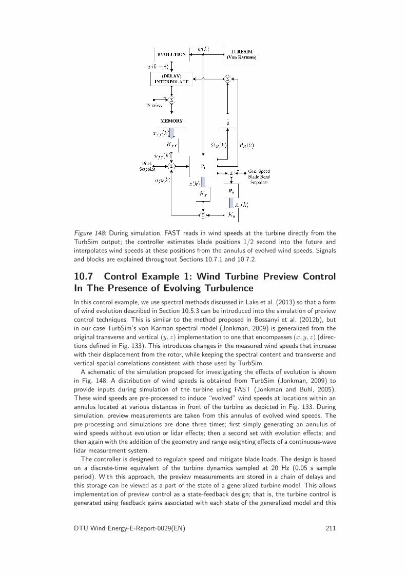
Figure 148: During simulation, FAST reads in wind speeds at the turbine directly from the

TurbSim output; the controller estimates blade positions 1/2 second into the future and

interpolates wind speeds at these positions from the annulus of evolved wind speeds. Signals

and blocks are explained throughout Sections 10.7.1 and 10.7.2.

10.7 Control Example 1: Wind Turbine Preview ControlIn The Presence of Evolving Turbulence

In this control example, we use spectral methods discussed in Laks et al. (2013) so that a form

of wind evolution described in Section 10.5.3 can be introduced into the simulation of preview

control techniques. This is similar to the method proposed in Bossanyi et al. (2012b), but

in our case TurbSim’s von Karman spectral model (Jonkman, 2009) is generalized from the

original transverse and vertical (y, z) implementation to one that encompasses (x, y, z) (direc-

tions defined in Fig. 133). This introduces changes in the measured wind speeds that increase

with their displacement from the rotor, while keeping the spectral content and transverse and

vertical spatial correlations consistent with those used by TurbSim.

A schematic of the simulation proposed for investigating the effects of evolution is shown

in Fig. 148. A distribution of wind speeds is obtained from TurbSim (Jonkman, 2009) to

provide inputs during simulation of the turbine using FAST (Jonkman and Buhl, 2005).

These wind speeds are pre-processed to induce “evolved” wind speeds at locations within an

annulus located at various distances in front of the turbine as depicted in Fig. 133. During

simulation, preview measurements are taken from this annulus of evolved wind speeds. The

pre-processing and simulations are done three times; first simply generating an annulus of

wind speeds without evolution or lidar effects; then a second set with evolution effects; and

then again with the addition of the geometry and range weighting effects of a continuous-wave

lidar measurement system.

The controller is designed to regulate speed and mitigate blade loads. The design is based

on a discrete-time equivalent of the turbine dynamics sampled at 20 Hz (0.05 s sample

period). With this approach, the preview measurements are stored in a chain of delays and

this storage can be viewed as a part of the state of a generalized turbine model. This allows

implementation of preview control as a state-feedback design; that is, the turbine control is

generated using feedback gains associated with each state of the generalized model and this


encompasses the storage of preview measurements. If the gains associated with the preview

storage are partitioned from the gains applied to turbine measurements, then the former

are correctly viewed as disturbance feedforward control and this is how they are depicted in

Fig. 148. In the course of design, it is determined that the majority of benefit of preview is

obtained using 0.5 s (10 samples) worth of feed-forward compensation, but this can change

depending on the dynamics of the turbine involved.

The FAST simulation code marches the TurbSim wind distribution past the turbine at

the mean speed of 18 m/s. The pre-processing induces evolution corresponding to distances

iTs × 18 where Ts is the sample period and i is the number of preview samples used. Where

the evolution distance is greater than 10Ts × 18, the process is equivalent to taking preview

measurements further in front of the turbine, and then waiting the appropriate amount of

time before applying the preview gains to the measurements.

10.7.1 H2 Optimal Preview Control

In this section, we describe the design of the preview controller and then evaluate its perfor-

mance in the presence of emulated wind evolution. Linear models are obtained from the FAST

wind turbine modeling code (Jonkman and Buhl, 2005) developed at NREL. The model is

based on a 40 m diameter, three-bladed controls advanced-research turbine (CART3) located

at NREL’s National Wind Technology Center (NWTC). The nominal operating point for de-

sign (and simulation) is a uniform wind of 18 m/s, a blade pitch of 12.7, and a rotor speed

of 41.7 rpm.

As in Laks et al. (2011b), the FAST linearizations are used to obtain a discrete-time state-

space model representing the turbine dynamics Pt with a 20 Hz sample rate. For controller

design, the linearized model includes a first-order generator degree of freedom (DOF), second-

order dynamics for each blade’s out-of-plane blade flap compliance, and a second-order drive-

train compliance. This model is then augmented with simple pitch actuator dynamics that

provide the pitch rates generated by individual pitch commands. During simulation, all DOFs

provided by FAST are used except for yaw and teeter (the freedom of the rotor to tilt).

In addition, integral control on generator speed error Ωg (= ΩRNgb where Ngb is the gear-

box ratio and ΩR is the rotor speed) and rejection of 1P variation in the bending moments are

obtained by augmenting the turbine model with additional dynamics Pa driven by measure-

ments of these signals. We configure the control system to use individual point measurements

of the longitudinal wind that the blades will encounter at 75% span after a fixed time delay

of i samples, where the point measurements rotate in unison with the blades. As discussed in

Laks et al. (2011b), this corresponds to using a blade-local model, that describes the effect

on the turbine of wind speed perturbations local to each blade.

The state feedback is designed by forming the generalized plant (the FAST linearization with

preview storage and augmented dynamics) with weighting on outputs that include generator

speed perturbations and perturbations in out-of-plane blade bending moments. The state-

feedback gains [Kx Ka Kff ] are optimized to minimize the H2 norm from the preview wind

measurement to weighted versions of flap and speed perturbations; this includes a penalty on

excessive pitch rates so that the associated linear quadratic regulator problem is well posed. It

is possible to compute the optimal state feedback independent of the amount of preview used

(Hazell, 2008). This involves using the stabilizing solution of a Riccati equation to compute

both the optimal state-feedback and feedforward gains. Details can be found in Laks et al.

(2013).

In formulating the H2 cost, emphasis is initially focused on the flap response to wind

perturbations. Then, the penalty on pitch effort is increased until the (linear) closed-loop

response to a step change in collective wind produces pitch rates on the order of 10/s.

Generally, the H2 performance improves with the number of samples of preview, but remains

bounded below so that there is a diminishing return; this lower bound is essentially reached

with the use of about 4 samples of preview at 20 Hz. However, the goal is not the precise

value of the H2 norm, but the attenuation of perturbations in blade load due to perturbations


Figure 149: Collective flap response to collective wind: dashed line indicates open loop (no

feedback control); each level of preview is indicated by the progression from blue to red.

The notch near 0.7 Hz corresponds to the rejection of 1P loading that is provided by the

augmented dynamics.

in wind speed. This goal is evident in the frequency responses provided in Fig. 149.

10.7.2 Controller Performance Simulations

As shown in Fig. 148, TurbSim is used to generate wind speeds at the turbine that are

consistent with the von Karman spectral model. Then the technique presented in Laks et al.

(2013) is used to induce evolved wind speeds located at 60 evenly spaced azimuths that are at

a measurement radius of r = 15 m (= 75% blade span). The evolution distance d = iTs×U

is chosen based upon i samples at the control system sample rate of 20 Hz (= 1/Ts) and the

nominal wind speed of U = 18 m/s.

The controller is simulated using feedback only, and also with increments of i samples of

preview

Kff =[Kw0 · · · Kwi 0 · · · 0

], (243)

up to i = 10 samples. For previews 0 ≤ i ≤ 10, the controller uses gains up through Kwi,

and for i > 10, the controller uses preview gains through Kw10. In the latter case, this is

equivalent to taking measurements further than 1/2 s (at 18 m/s average wind speed) ahead

of the turbine, and then waiting until those wind speeds are within 1/2 s of reaching the

turbine before storing them in the feedforward MEMORY.

The controller is simulated using the same base TurbSim wind field first using feedback only,

and then multiple times using feedback plus preview feedforward. For the preview simulations,

evolved wind speed measurements are pre-computed for the base wind field at distances

that correspond to preview times in the range [0.05,10] s (or preview distances in the range

[0.9,180] m). The computation done for each distance produces 60 time-varying measurement

waveforms arranged spatially in a ring in front of the turbine as depicted in Fig. 133. As

indicated in Fig. 148, the present rotor position θR(k) and speed ΩR(k) are used to predict

1/2 s worth of blade rotation, and then the evolved wind speeds at the 60 azimuth locations

are interpolated to the predicted blade positions. This gives the controller a preview of wind

speeds that the blades will encounter over a 1/2 s horizon.

There are three sets of measurements generated corresponding to (i) an ideal preview

case without evolution, (ii) a set that includes the evolution model, and (iii) a set that

uses evolution and lidar distortion as discussed in Section 10.5. The turbine and controller

simulation is repeated for each set of pre-computed wind measurements and the RMS blade

load and preview measurement error (relative to the wind at the blades) are computed. The


Figure 150: The accuracy (top plot) of evolved preview measurements w/o lidar distortion

(blue/dots) and with lidar distortion (green/diamonds); RMS blade-loads (lower plot) w/o

lidar distortion (blue/dots) and with lidar distortion (green/diamonds).

results are provided in Fig. 150. Simply introducing a set of wind speeds in the annulus that

are properly correlated with the existing TurbSim field without evolution results in a base

level of error relative to the wind speeds actually encountered by the blades; this is depicted

by the red-dashed line in the top plot of Fig. 150.

10.7.3 Simulation Results

Given the 0.7 m/s RMS base level of measurement error, the maximum benefit potential of

preview actuation is about a 10% drop in RMS blade flap relative to feedback-only control

as shown in the lower plot of Fig. 150. As expected, the benefit of preview in terms of RMS

blade loading reaches a maximum with 0.2 s (4 samples) of preview time. Without evolution

or lidar effects, preview greater than 0.2 s does not really improve performance. With evolution

and no lidar distortion, blade load mitigation performance deteriorates with preview distances

greater than 0.2 s as measurement errors increase with distance from the rotor due to the

applied evolution. Because of the frequency dependent nature of the evolution model, these

measurement errors tend to be more significant at higher frequencies leading to over-actuation

by the feedforward control. By 10 s (180 m) of preview, the advantage of preview control

relative to feedback-only has been completely lost.

When applying preview based on a lidar measurement, large cone angles relative to the x

(downstream) direction result in significant contributions of the transverse v and vertical w

wind components to the estimate u of the downstream speed. This is apparent in the sharp

upward trend of the green-diamond curve as preview times are reduced below 3 s (< 54 m

preview, or equivalently a cone angle > 15); at these shorter preview distances the geometry

errors dominate the preview measurement errors. At larger preview times, evolution dominates

the lidar measurement error, but the system is benefiting from the lidar range weighting, which

low-pass filters the poorly correlated high frequencies in the wind. What is surprising is the

magnitude of the effect this filtering has on the quality of the load mitigation. Since the


10−10

10−5

100

105

gen s

peed

10−4

10−3

10−2

10−1

100

10−10

100

bla

de p

itch

Bode Diagram

Frequency (Hz)

Magnitude (

abs)

feedback only

typical measurement

perfect measurement

Figure 151: Frequency responses of closed-loop transfer functions, with wind spectrum in-

cluded, showing generator speed error and blade pitch actuation with H2 optimal combined

feedforward/feedback control for the NREL 5-MW turbine at a 13 m/s wind speed operating

point with 9 seconds of available preview time.

lidar is removing high frequency content from the measurement, the remaining low frequency

errors due to evolution do not become significant until at least 7 s (126 m) of preview, when

even the low frequencies of turbulence have significantly evolved. Additional details regarding

this control study can be found in Laks et al. (2013).

10.8 Control Example 2: H2 Optimal Control with Modelof Measurement Coherence

In this section, an H2 optimal controller design is described where a model of wind mea-

surement coherence is included in the design process. This combined feedforward/feedback

controller is designed to minimize a weighted sum of RMS generator speed error and RMS

blade pitch (deviation from the operating point) using the NREL 5-MW model, assuming the

Kaimal wind spectrum, class B turbulence (medium turbulence) and the normal turbulence

model (NTM) (Jonkman, 2009).

Figure 151 shows the resulting closed-loop generator speed and pitch actuation responses

for three different cases: feedback only, typical measurements (measurement coherence is

modeled as the magnitude squared of a single-pole low-pass filter with bandwidth of 0.2 Hz),

and perfect measurements. We see that with lidar measurements, generator speed error is

improved at both low and high frequencies, and pitch actuation is reduced at high frequencies.

Figure 152 shows the magnitudes of the optimal controllers. As the lidar measurement

improves, the feedforward controller action increases at low frequencies, and the feedback

controller action decreases at low frequencies, freeing it to act more at mid frequencies if

necessary. The decrease in low-frequency feedback action is helpful because feedback control

performance is fundamentally limited by the Bode sensitivity integral (Franklin et al., 2006),

which essentially says that a decrease in sensitivity to disturbance at one frequency must be

balanced by an increase in sensitivity to disturbance at another frequency. When feedforward

takes over at low frequencies, feedback can increase sensitivity to low-frequency disturbance,

and therefore can decrease sensitivity to mid-frequency disturbance. Thus low-frequency wind

measurements can lead to reductions in mid-frequency loads. This increase in mid-frequency

feedback action occurs for typical lidar measurements, but for perfect measurements, feedback

is unnecessary because the feedforward controller takes over at all frequencies, assuming


10−4

10−2

100

0

0.005

0.01

0.015

0.02

0.025

0.03

0.035

0.04

0.045

0.05From: wind meas

To: bla

de p

itch

10−4

10−2

100

From: gen speedBode Diagram

Frequency (Hz)

Magnitude (

abs)

feedback only

typical measurement

perfect measurement

Figure 152: Frequency responses of H2 optimal feedforward (From: wind meas) and feedback

(From: gen speed) controllers for the NREL 5-MW turbine at a 13 m/s wind speed operating

point, with 9 seconds of available preview time.

perfect knowledge of the turbine model.

10.9 Summary

This chapter presented an introduction to wind turbine control using lidar, primarily focusing

on a frequency domain analysis of lidar measurement quality. Two control examples were

included to highlight the challenges that accompany the design of feedforward controllers

that use lidar measurements. A summary of the main results presented in this chapter is

provided here.

• With perfect preview measurements of wind speeds, a model-inverse feedforward con-

troller can completely cancel the effect of the wind disturbance on a turbine variable

of interest, assuming perfect turbine modeling. For imperfect preview measurements, a

measurement filter can be introduced such that the mean square value of the turbine

variable is minimized.

• A feedforward control system requires not only measurements of the wind disturbance,

but also a certain amount of preview time required for implementation.

• For blade pitch control, the lidar system should be used to acquire an estimate of the

“blade effective wind speed,” a weighted integral of wind speeds along the blade that

describes the equivalent wind speed experienced by the blade. Furthermore, the longi-

tudinal component of the wind is of interest because it has the greatest impact on the

rotor aerodynamics.

• The two main sources of lidar measurement error are geometry effects, or estimation

of the longitudinal component using a line-of-sight measurement, and wind evolution,

which represents the decorrelation of the turbulence as it travels downwind between the

measurement location and the turbine. Spatial averaging, inherent in lidar measurements,

appears to help with estimation of blade effective wind speed.

• Wind turbine control systems are often defined in the non-rotating frame, where estimates

of the collective, vertical shear, and horizontal shear wind components are required, as

opposed to measurements of the wind speed at individual blades.


• Measurement coherence, which can be calculated given a frequency domain wind field

model, can be used to find the optimal lidar measurement configuration that minimizes

the mean square value of a turbine variable of interest.

• For a hub-mounted lidar, there is an optimal preview distance that minimizes measure-

ment error. For shorter preview distances, geometry effects cause error to increase. Be-

yond the optimal preview distance, wind evolution becomes more severe, thus increasing

measurement error.

• A combined feedback/feedforward control system can be optimized given the measure-

ment coherence. For perfect measurement coherence, the control system relies entirely

on the feedforward controller. For measurements that are completely uncorrelated with

the wind disturbance, the control system relies entirely on feedback. For imperfect mea-

surements that have some correlation with the wind disturbance, the optimal control

strategy utilizes both feedback and feedforward control.

Notation

1P once per revolution

CPSD Cross-Power Spectral Density

CW continuous-wave

CP (r) radially-dependent coefficient of power

CQ(r) radially-dependent coefficient of torque

d measurement preview distance

DEL Damage Equivalent Load

f frequency (Hz)

F feedforward controller

Fℓ lidar focus distance

h hub height

Hpre lidar measurement prefilter

IEC International Electrotechnical Commission

Ka state feedback gains for augmented states

Kff state feedback gains for preview measurements

Kx state feedback gains for turbine states~ℓ lidar direction vector

NREL National Renewable Energy Laboratory

Ngb gear box ratio

PSD Power Spectral Density

Pa augmented dynamics

Pt wind turbine dynamics

r lidar scan radius

R rotor radius

Rℓ range along lidar beam

RMS root mean square

STD standard deviation

Saa(f) power spectral density of signal a

Sab(f) cross-power spectral density between signals a and b

Ts sample period of control system

Tywt transfer function from wind disturbance to output y

TyβFFtransfer function from feedforward blade pitch command to output y

u longitudinal wind speed

U mean wind speed

ublade blade effective wind speed

uhh hub height or collective wind speed component

uhh estimate of hub height wind speed component from lidar measurements

urotor rotor effective wind speed

uwt,los range weighted line-of-sight measurement

u estimate of u component from lidar measurement

~uwt range weighted wind speed vector

v transverse wind speed

w vertical wind speed


Wb(r) blade effective weighting function

W (Fℓ, Rℓ) lidar range weighting function

wm wind speed disturbance preview measurement

wt wind disturbance at the turbine

x longitudinal (along-wind) direction

y transverse (horizontal) direction; output error variable from the turbine

y0 collective component of output error variable from the turbine

yh horizontal component of output error variable from the turbine

yv vertical component of output error variable from the turbine

z vertical direction

γ2ab(f) coherence between signals a and b

∆h horizontal shear wind speed component

∆h estimate of horizontal shear component from lidar measurements

∆v vertical shear wind speed component

∆v estimate of vertical shear component from lidar measurements

θR rotor position

ψ azimuth angle in rotor plane

Ωg generator speed

ΩR rotor speed

ReferencesBir, B. (2008) Multiblade coordinate transformation and its application to wind turbine analysis. Proc. AIAA

Aerospace Sciences Meeting, Reno, NV

Bossanyi, E. A. (2005) Further load reductions with individual pitch control. Wind Energy 8:481–485

Bossanyi, E. A. (2012) Un-freezing the turbulence: Improved wind field modeling for investigating lidar-assisted

wind turbine control. Proc. European Wind Energy Association Annual Event (EWEA), Copenhagen, Den-

mark

Bossanyi, E. A., Kumar, A., and Hugues-Salas, O. (2012b) Wind turbine control applications of turbine-

mounted lidar. Proc. Science of Making Torque from Wind, Oldenburg, Germany

Dunne, F., Pao, L. Y., Wright, A. D., Jonkman, B., Kelley, N., and Simley, E. (2011a) Adding feedforward

blade pitch control for load mitigation in wind turbines: Non-causal series expansion, preview control, and

optimized FIR filter methods. Proc. AIAA Aerospace Sciences Meeting, Orlando, FL

Dunne, F., Pao, L. Y., Wright, A. D., Jonkman, B., and Kelley, N. (2011b) Adding feedforward blade pitch

control to standard feedback controllers for load mitigation in wind turbines. Mechatronics 21:682–690

Dunne, F., Schlipf, D., Pao, L. Y., Wright, A. D., Jonkman, B., Kelley, N., and Simley, E. (2012) Comparison

of two independent LIDAR-based pitch control designs. Proc. AIAA Aerospace Sciences Meeting, Nashville,

TN

Franklin, G. F., Powell, J. D., and Emami-Naeini, A. (2006) Feedback control of dynamic systems, fifth edition,

Pearson Prentice Hall

Frehlich, R. and Kavaya, M. (1991) Coherent laser performance for general atmospheric refractive turbulence.

Applied Optics 30:5325–5352

Frehlich, R., Meillier, Y., Jensen, M., Balsley, B. and Sharman, M. (2006) Measurements of boundary layer

profiles in an urban environment. Applied Meteorology and Climatology 45:821–837

Harris, M., Hand, M., and Wright, A. (2005) Lidar for turbine control, NREL/TP-500-39154, Tech. Rep.,

National Renewable Energy Laboratory, Golden, CO

Harris, M., Bryce, D., Coffey, A., Smith, D., Birkemeyer, J., and Knopf, U. (2007) Advance measurements of

gusts by laser anemometry. Wind Engineering and Industrial Aerodynamics 95:1637–1647

Hazell, A. (2008) Discrete-Time Optimal Preview Control, Ph.D. Thesis, Imperial College, University of

London, London, England

IEC (2001) IEC 61400-13 Ed. 1: Wind turbine generator systems: Measurement of mechanical loads. Int.

Electrotechnical Commission

IEC (2005) IEC 61400-1 Ed. 3: Wind turbines - Part 1: Design requirements. Int. Electrotechnical Commission

Jonkman, J. and Buhl, M. (2005) FAST user’s guide, NREL/TP-500-38230, Tech. Rep., National Renewable

Energy Laboratory, Golden, CO


Jonkman, B. (2009) TurbSim user’s guide: Version 1.50, NREL/TP-500-46198, Tech. Rep., National Renew-

able Energy Laboratory, Golden, CO

Jonkman, J., Butterfield, S., Musial, W., and Scott, G. (2009) Definition of a 5-MW reference wind turbine for

offshore system development, NREL/TP-500-38060, Tech. Rep., National Renewable Energy Laboratory,

Golden, CO

Kodama, N., Matsuzaka, T., Tuchiya, K., and Arinaga, S. (1999) Power variation control of a wind generator

by using feed-forward control. Renewable Energy 16:847–850

Kragh, K. A., Hansen, M. H., and Mikkelsen, T. (2013) Precision and shortcomings of yaw error estimation

using spinner-based light detection and ranging. Wind Energy 16:353–366

Kristensen, L. (1979) On longitudinal spectral coherence. Bound.-Layer Meteorol. 16:145–153

Laks, J., Pao, L. Y., Simley, E., Wright, A. D., Kelley, N., and Jonkman, B. (2011a) Model predictive control

using preview measurements from lidar. Proc. AIAA Aerospace Sciences Meeting, Orlando, FL

Laks, J., Pao, L. Y., Wright, A. D., Kelley, N., and Jonkman, B. (2011b) The use of preview wind measurements

for blade pitch control. Mechatronics 21:668–681

Laks, J., Simley, E., and Pao, L. Y. (2013) A spectral model for evaluating the effect of wind evolution on

wind turbine preview control. Proc. American Control Conference, Washington, D.C.

Mikkelsen, T. (2009) On mean wind and turbulence profile measurements from ground-based wind lidars:

limitations in time and space resolution with continuous wave and pulsed lidar systems. Proc. European

Wind Energy Conference, Stockholm, Sweden

Mikkelsen, T., Angelou, N., Hansen, K., Sjoholm, M., Harris, M., Slinger, C., Hadley, P., Scullion, R., Ellis,

G., and Vives, G. (2013) A spinner-integrated wind lidar for enhanced wind turbine control. Wind Energy

16:625–643

Mirzaei, M., Soltani, M., Poulsen, N. K., and Niemann, H. H. (2013) Model predictive control of wind turbines

using uncertain lidar measurements. Proc. American Control Conference, Washington, D.C.

Moriarty, P.J. and Hansen, A.C. (2005) Aerodyn Theory Manual, NREL/TP-500-36881, Tech. Rep., National

Renewable Energy Laboratory, Golden, CO

Pao, L. Y. and Johnson, K. E. (2011) Control of wind turbines: Approaches, challenges, and recent develop-

ments. IEEE Control Systems Magazine 31:44–62

Pedersen, A. T., Sjoholm, M., Angelou, N., Mikkelsen, T., Montes, B. F., Pedersen, J. E., Slinger, C., and

Harris, M. (2013) Full-scale field test of a blade-integrated dual-telescope wind lidar. Proc. European Wind

Energy Association Annual Event (EWEA), Vienna, Austria

Rettenmeier, A., Bischoff, O., Hofsaß, M., Schlipf, D., and Trujillo, J. J. (2010) Wind field analysis using a

nacelle-based LIDAR system. Proc. European Wind Energy Conference, Warsaw, Poland

Schlipf, D. and Kuhn, M. (2008) Prospects of a collective pitch control by means of predictive disturbance

compensation assisted by wind speed measurements. Proc. German Wind Energy Conference (DEWEK),

Bremen, Germany

Schlipf, D., Trujillo, J. J., Basterra, V., and Kuhn, M. (2009) Development of a wind turbine lidar simulator.

Proc. European Wind Energy Conference, Marseille, France

Schlipf, D., Schuler, S., Grau, P., Allgower, F., and Kuhn, M. (2010) Look-ahead cyclic pitch control using

LIDAR. Proc. Science of Making Torque from Wind, Heraklion, Greece

Schlipf, D., Kapp, S., Anger, J., Bischoff, O., Hofsaß, M., Rettenmeier, A., Smolka, U., and Kuhn, M. (2011)

Prospects of optimization of energy production by lidar assisted control of wind turbines. Proc. European

Wind Energy Association Annual Event (EWEA), Brussels, Belgium

Schlipf, D., Mann, J., Rettenmeier, A., and Cheng, P. W. (2012a) Model of the correlation between lidar

systems and wind turbines for lidar assisted control. Proc. Int. Symp. for the Advancement of Boundary

Layer Remote Sensing, Boulder, CO

Schlipf, D., Schlipf, D. J., and Kuhn, M. (2012b) Nonlinear model predictive control of wind turbines using

LIDAR. Wind Energy

Scholbrock, A. K., Fleming, P . A., Fingersh, L. J., Wright, A. D., Schlipf, D., Haizman, F., and Belen, F.

(2013) Field testing LIDAR based feed-forward controls on the NREL controls advanced research turbine.

Proc. AIAA Aerospace Sciences Meeting, Grapevine, TX


Simley, E., Pao, L. Y., Kelley, N., Jonkman, B., and Frehlich, R. (2012) LIDAR wind speed measurements of

evolving wind fields. Proc. AIAA Aerospace Sciences Meeting, Nashville, TN

Simley, E. and Pao, L. Y. (2013a) Correlation between rotating LIDAR measurements and blade effective

wind speed. Proc. AIAA Aerospace Sciences Meeting, Grapevine, TX

Simley, E. and Pao, L. Y. (2013b) Reducing lidar wind speed measurement error with optimal filtering. Proc.

American Control Conference, Washington, D.C.

Simley, E., Pao, L. Y., Frehlich, R., Jonkman, B., and Kelley, N. (2013c) Analysis of light detection and

ranging wind speed measurements for wind turbine control. Wind Energy

Slinger, C. and Harris, M. (2012) Introduction to continuous-wave Doppler lidar. Proc. Summer School in

Remote Sensing for Wind Energy, Boulder, CO

Wang, N., Johnson, K., and Wright, A. (2012a) Combined feedforward and feedback controllers for turbine

power capture enhancement and fatigue loads mitigation with pulsed lidar. Proc. AIAA Aerospace Sciences

Meeting, Nashville, TN

Wang, N., Johnson, K., and Wright, A. (2012b) FX-RLS-based feedforward control for lidar-enabled wind

turbine load mitigation. IEEE Transactions on Control Systems Technology 20:1212–1222

WT Perf (2012). NWTC Design Codes (WT Perf by Andrew Platt).

http://wind.nrel.gov/designcodes/simulators/wtperf/. Last modified 26-November-2012


10 Lidars and wind turbine control – Part...

Documents

Transcript of 10 Lidars and wind turbine control – Part...