1 , V.V.Konichek , I.Ye.Sinelnikov , O.M.Burkhonov , B.P ...

arX

iv:a

stro

-ph/

0312

631v

1 2

9 D

ec 2

003

Astronomy & Astrophysics manuscript no. aa˙0104 May 7, 2021(DOI: will be inserted by hand later)

Color Effects Associated with the 1999 Microlensing Brightness

Peaks in Gravitationally Lensed Quasar Q2237+0305

V.G.Vakulik1, R.E.Schild2, V.N.Dudinov1, A.A.Minakov3 , S.N.Nuritdinov4, V.S.Tsvetkova3,A.P.Zheleznyak1, V.V.Konichek1, I.Ye.Sinelnikov1, O.M.Burkhonov4, B.P.Artamonov5, and V.V.Bruevich5

1 Institute of Astronomy of Kharkov National University, Sumskaya 35, 61022 Kharkov, Ukraineemail: [email protected]

2 Center for Astrophysics, 60 Garden Street, Cambridge, MA 02138, U.S.A.email: [email protected]

3 Institute of Radio Astronomy of Nat.Ac.Sci. of Ukraine, Chervonoznamennaya 4, 61002 Kharkov, Ukraineemail: [email protected]

4 Ulugh Beg Astronomical Institute of Ac.Sci. of Uzbekistan, Astronomicheskaya 33, 700052, Tashkent, Republicof Uzbekistanemail: [email protected]

5 Sternberg Astronomical Institute, Universitetski Ave. 13, 119899 Moscow, Russiaemail: [email protected]

Received ...; accepted ...

Abstract. Photometry of the Q2237+0305gravitational lens in VRI spectral bands with the 1.5-m telescope ofthe high-altitude Maidanak observatory in 1995-2000 is presented. Monitoring of Q2237+0305 in July-October2000, made at nearly daily basis, did not reveal rapid (night-to-night and intranight) variations of brightness ofthe components during this time period. Rather slow changes of magnitudes of the components were observed,such as 0.08m fading of B and C components and 0.05m brightening of D in R band during July 23 - October7, 2000. By good luck three nights of observation in 1999 were almost at the time of the strong brightness peakof image C, and approximately in the middle of the ascending slope of the image A brightness peak. The Ccomponent was the most blue one in the system in 1998 and 1999, having changed its (V-I) color from 0.56m to0.12m since August 1997, while its brightness increased almost 1.2m during this time period. The A componentbehaved similarly between August 1998 and August 2000, having become 0.47m brighter in R, and at the sametime, 0.15m bluer. A correlation between the color variations and variations of magnitudes of the componentsis demonstrated to be significant and reaches 0.75, with a regression line slope of 0.33. A color (V-I) vrs color(V-R) plot shows the components settled in a cluster, stretched along a line with a slope of 1.31. Both slopesare noticeably smaller than those expected if a standard galactic interstellar reddening law were responsible forthe differences between the colors of images and their variations over time. We attribute the brightness and colorchanges to microlensing of the quasar’s structure, which we conclude is more compact at shorter wavelengths, aspredicted by most quasar models featuring an energizing central source.

Key words. cosmology: gravitational lensing – galaxies: quasars: individual: QSO 2237+0305 – methods: observa-tional – techniques: image processing

1. Introduction

The Q2237+0305 gravitational lens (the Einstein Cross) isone of the most impressive manifestations of the gravita-tional lensing phenomenon - four images of the same high-redshift quasar (z = 1.695) are arranged almost symmetri-cally around the lensing galaxy nucleus (z = 0.039) withina circle of approximately 2′′ diameter. The Q2237+0305system is an excellent target to study microlensing events,

Send offprint requests to: V.Vakulik

because the light beams, corresponding to the 4 lensedquasar’s images, pass through the interior, heavily pop-ulated part of the lensing galaxy and thus, have a highprobability to intersect a significant mass of microlens-ing stars as they pass through the inner disc (Kayser &Refsdal 1989).

The system has been intensively examined since 1987,when the first published measurements of magnitudes ofthe individual lensed quasar components in g, r and iGunn filters were made by Yee (1988). The first attempt to

http://arxiv.org/abs/astro-ph/0312631v1

2 V.Vakulik et al.: Color effects in Q2237+0305

build the light curves of the four quasar components wasmade in 1991 by Corrigan et al. (1991). They brought to-gether all the available Q2237 images of sufficient quality,taken with different telescopes and in a variety of pass-bands, - Mould B, V and R and Gunn g, r and i, - andreprocessed with a single algorithm. Having used the mul-ticolor photometry data for 33 normal stars, whose (B−V )colors ranged from -0.3 to 1.5, they calculated the relevantcolor equations, which allowed them to reduce all the ob-servations to a single passband. Their r Gunn and B lightcurves cover the time period from September 1986 up toDecember 1989, and include the first microlensing eventobserved in August 1988 by Irwin et al. (1989).

A further attempt to use all the available observationaldata for Q2237+0305 was made in 1994 by construct-ing ”differential” light curves, which were argued to befree from the effects of different spectral bands, techniqueof zero-pointing, and the quasar intrinsic brightness vari-ations, (Houde et al. 1994). In addition to the data of1986-89, contained in (Corrigan et al. 1991), other resultswere used, taken in 1990 and 1991 by Crane et al. (1991),Racine (1992), Rix et al. (1992), and Houde et al. (1994).

The first program of regular photometric monitoringof Q2237+0305 was started in 1990 at the Nordic OpticalTelescope, (Østensen et al. 1996). A large number of mea-surements of the four quasar components in V,R and Ispectral bands during five years were obtained, which per-mitted construction, with the use of Corrigan et al. (1991)zero-pointing, of the historic light curves, covering 9 yearsof observations.

No regular multi-filter monitoring of Q2237+0305 isreported between 1996 and 1999, excepting our resultsof V RI photometry for three nights on 17-19 September1995, (Vakulik et al. 1997), and the similar results byBurud et al. (1998), obtained with the Nordic OpticalTelescope for a close epoch, 10-11 October 1995. No night-to-night or intranight brightness variations of the fourcomponents have been found for these time periods, whilea noticeable change in the component B color as comparedto the observations by Yee in 1987 (1988) has been re-ported in both works. A short time-scale monitoring withthe CFHT in June 14-16, 1992 should be mentioned here,(Cumming & De Robertis, 1995), which also did not re-veal any photometric variations in R and I bands duringa three-day period.

In 1999 and 2000, the results of V RI photometry in1997 and 1998 with the Maidanak 1.5-m telescope werepublished, (Bliokh et al. 1999) and (Dudinov et al. 2000a).Recently, the superb results of a detailed long-term moni-toring, obtained within the OGLE program from 4 August1997 to 5 November 2000 has become publicly accessi-ble, and partly presented in two papers of Wozniak et al.(2000a) and (2000b). And in 2002, the results of moni-toring of Q2237+0305 by GLITP collaboration appeared,which cover the 4-month period October 1999 - February2000 (Alcalde et al. 2002). The most recent publication ofthe results of low-resolution observations with the 3.5-mtelescope at the Apache Point Observatory should be also

mentioned here, (Schmidt et al. 2002), which have giventhe Gunn r lightcurves of A and B components for 73dates between July 1995 and January 1998. In spite of arather low photometric accuracy, - an error bar of 0.1m to0.2m is reported, - the data are of value first of all becausethey include the brightness peak of A component in 1996.As far as we know, no more data about this event havebeen ever published, though reported in private commu-nication, (e.g. R. Østensen).

The brightness records taken in broad-band filters area good starting point for theorists to estimate the sizeof the quasar radiating region in the visual (ultravioletrest frame) continuum, and to determine the range formicrolens masses responsible for the observed brightnessvariations. Both the statistical analysis of long-term mon-itoring data, and simulation of the isolated microlens-ing peaks have been applied to calculate these values,(Nadeau et al. 1991, Lewis & Irwin 1996, Refsdal & Stabell1993, Webster et al. 1991, Wyithe et al. 2000a, Wyitheet al, 2000b, Wyithe et al. 2002, Yonehara 2000), havinggiven the estimates of the quasar dimension, - 1015cm to1016cm in the optical continuum, and a great variety of mi-crolens masses ranging from 0.0006M⊙ < M < 0.006M⊙,(Nadeau et al. 1991), to 0.1M⊙, (Wambsganss 1991), allindicating however, that microlensing events in the systemare mostly caused by subsolar-mass objects.

These available models confront a problem which prob-ably indicates a breakdown of the simple assumption thatthe luminous quasar is a uniformly bright accretion disc.The dilemma is that the short time scale of the observedevents like the C image peak in July 1999 and the A bright-ness peak in November 1999 occur on such short timescales that small accretion disc diameters are implied; suchsmall bright accretion discs would have occasional strongbrightness peaks of several magnitudes that are never ob-served. This probably tells us that a more complex modelwhere the time scale of the brightness peaks is related toa quasar structure crossing time, not the crossing time ofthe entire quasar luminosity. We expect to apply, in a sub-sequent report, the Schild and Vakulik (2003) double ringquasar model that successfully models the long history ofQ0957+561 microlensing observations.

No systematic multicolor photometric measurementsexisted until the monitoring program with the NOT wasstarted in 1990 (Østensen et al. 1996). Meanwhile, a sus-picion was expressed by Corrigan et al. in 1991, and in1992 by Rix et al. independently (Corrigan et al. 1991,Rix et al. 1992), that the color indices of the componentsmight have changed since the first three-color observationsby Yee, (1988). It was a very important statement, sincereducing different datasets to a single light curve, (e.g.Houde et al., 1994), as well as determining the extinctionlaw in the Q2237+0305 lensing galaxy, (Yee 1988, Nadeauet al. 1991, Falco et al. 1999), are substantially based onthe assumptions, that ”all four components have identicalintrinsic color indices”, and ”their observed color differ-ences are due to different degrees of interstellar extinc-tion and reddening by the same extinction law”, (Houde

V.Vakulik et al.: Color effects in Q2237+0305 3

et al. 1994), and ”the magnification is wavelength inde-pendent... and time independent”, (Falco et al. 1999). Inparticular, Falco et al. (1999) measured the value of RV

for Q2237+0305 to be equal 5.3 and came to a conclusionabout great differences in the extinction laws for lensinggalaxies from a sample consisting of 23 gravitational lenssystems. However, as it can be seen from Fig. 4 in Falcoet al. (1999), the differences may be significant at wave-lengths shorter than 550nm, while at larger wavelengthsthe difference between the extinction curves does not ex-ceed the error bars.

In discussing the results of the five-year V RI moni-toring of Q2237+0305, Østensen et al. (1996) did not an-alyze, however, any color changes in the system, havingnoted only ”very nearly equal” colors for the componentsA and B, as well as roughly equal colors of C and D, withthe extinction difference between the pairs of 0.6m in Vband, provided the extinction law follows λ−1, accordingto Houde et al. (1994). Meanwhile, Vakulik et al. (1997)and Burud et al. (1998) reported that the B componentbecame the most blue one in the system in 1995, as com-pared to observations by Yee in 1987, (Yee 1988).

The next step in determining colors and color changesin the Q2237+0305 system was made in V RI observa-tions with the Maidanak 1.5-m telescope in 1997-1998,presented in Dudinov et al. 2000a and Dudinov et al.2000b. Variations of colors were argued to be significant,and a tendency of the components to become bluer as theirbrightness increased has been demonstrated with the useof all available multicolor data. Unfortunately, the remark-able monitoring by Wozniak et al. 2000a and Wozniak etal. 2000b has been made only in V band, and thus can notbe used to investigate the color changes, while the mostrecent data of the GLITP collaboration have been taken inV and R filters for a campaign of 4 months only (Alcaldeet al. 2002).

By this time, a great amount of observations ofQ2237+0305 in spectral ranges other than visual contin-uum exists, - VLA observations at 20cm and 3.6cm (Falcoet al. 1996), observations in the near and mid-IR (Nadeauet al. 1991; Agol et al. 2000), and in the quasar emissionlines (Fitte & Adam 1994; Racine 1992; De Robertis & Yee1988, Lewis et al. 1998, Saust 1994). The observed mag-nitudes of the components have been found to be almostunaffected by microlensings in these spectral ranges, whichindicates that much larger quasar features radiate in IRand in the radio, as well as in the emission lines, as com-pared to the optical continuum. The recent detection of anarc of C III] emission, connecting A, D and B components(Mediavilla et al. 1998), should be regarded as a visualproof of the extended emission line region of the source.Because of the low sensitivity of a large source bright-ness to microlensing, the brightness ratios for the compo-nents, measured in these spectral ranges, were used to testthe validity of a great variety of the existing macrolensingmodels, listed by Wyithe et al. (2002).

Observations in UV with the HST (Blanton et al. 1998)and the recent X-ray imaging of Q2237+0305 with the

Chandra X-ray Observatory (Dai et al. 2003) should bealso mentioned here, which provided, in particular, highlyaccurate relative coordinates of the components (Blantonet al. 1998) and the upper limits for the physical size andbrightness of the Broad-Line Region producing Ly-α emis-sion, (Dai et al. 2003). Also, the Chandra data permittedcalculation of the time delay between the A and B com-ponents of 2.7 hours.

2. Observations

Our observations were carried out with the 1.5-m AZT-22 telescope of the high-altitude Maidanak observatory,(Central Asia, Republic of Uzbekistan), known for its su-perb seeing conditions and a large number of cloudlessnights, (Ehgamberdiev et al. 2000). Because of technicalreasons, we had to use three different CCD cameras in ourobservations, Pictor-416 camera in 1995, Pictor-416 andTI 800 x 800 cameras in 1997 and 1998, and ST-7 camerain 1999 and 2000. And because of technical reasons again,both f/8 and f/16 focal lengths were used in observations.The LN-cooled TI 800 x 800 camera, with pixel size of15µ, kindly provided by Prof.D.Turnshek, unfortunatelyrevealed some peculiarities, caused by the charge trans-fer inefficiency, that is characteristic for the CCD’s of thisgeneration, (Turnshek et al. 1997). In particular, notice-able stretching of stellar images in the direction of chargetransfer is observed, as well as a dependence of the PSFupon coordinates at the chip plane. In addition, sensitivityirregularities of the chip can not be corrected satisfactorily,with the output of the flatfielding procedure dependent onthe signal level. All these peculiarities reduced the actualaccuracy of photometry, that is seen in Tables 4 and 6.

Unfortunately, a poor telescope tracking systemspoiled the intrinsically good seeing of Maidanak sitesometimes and did not permit use of exposures longerthan 3 minutes. To provide sufficiently high accuracy ofour photometry with such short exposures, we took imagesin series, consisting of 10 to 20 frames each. The frameswere averaged before being subjected to photometric pro-cessing, while a comparison of photometry of individualframes enabled us to obtain an adequate estimate of therandom error inherent in a particular series.

Most of images has been taken in R band, - 31 datesin 1995-1999, (Table 4), plus 46 dates in 2000, (Table 5)- which were obtained almost at a daily basis during 2.5months. There is also photometry in V and I bands for 17dates in 1995-2000, (Table 6). Some results have been pre-sented in our previous publications (Vakulik et al. 1997,Bliokh et al. 1999, Dudinov et al. 2000a, Dudinov et al.2000b). We present here the results of all our observa-tions, including those which have been never published.In particular, the observations of July-October 2000 arepresented, which have been undertaken to search for short-period (night-to-night) variations of brightness. The ap-pearance of the Einstein Cross at six epochs betweenOctober 1995 and August 2001 can be seen in Fig. 1,


which clearly demonstrates high photometric variabilityin the system.

In addition to magnitudes of the components, the see-ing conditions are also presented in Tables 4 and 5, - thevalues of FWHM for particular nights, the scales and theCCD camera used.

3. Photometric Reductions

The difficulties inherent in accurate photometry ofground-based images of Q2237+0305, have been noted bymany authors, (Burud et al. 1998, Corrigan et al. 1991,Vakulik et al. 1997, Yee 1988). They are due mainly toits extremely compact spatial structure, with the wingsof the quasar images overlapping even under good seeingconditions. Additional difficulties are due to the presenceof a rather bright foreground lensing galaxy, with its steepradial brightness distribution. These are the main reasonsfor poor agreement of the results of different monitoringprograms, and even for a noticeable discrepancy in pho-tometric results for the same data reduced with differentalgorithms, (Burud et al. 1998, Alcalde et al. 2002). Inphotometry of the data of 1995-1999, we used the methoddescribed in Vakulik et al. 1997, and Bliokh et al. 1999,which is in general features similar to the double iterativePSF subtraction method, proposed by Yee (1988), whowas the first to present spatially resolved photometry ofthe system. In short, the method consists of the following.

The PSF estimate is obtained from a reference starimage, and is further superimposed upon each image com-ponent and the galaxy nucleus alternately, and then sub-tracted in such a way, that no depressions would appearin the residual brightness distribution. Such a procedureis repeated iteratively until a stable convergence of esti-mates of brightness and coordinates of the componentsis achieved. Then, according to the resulting estimates,the quasar components are subtracted, and the residualgalaxy brightness distribution is smoothed with a ratherbroad median filter. After the resulting galaxy bright-ness distribution is subtracted from the initial image, re-moval of quasar components is repeated, followed again bysmoothing the galaxy brightness distribution with a suc-cessively decreasing window. The iterative process stopswhen the width of the median filter becomes of order ofthe PSF width.

In processing our data for the 2000 observing season,another method was applied, which used the known rel-ative coordinates of the components and an analyticalmodel of the brightness distribution in the galaxy, repre-sented as a sum of three two-dimensional Gaussian func-tions. Before describing the algorithm, consider the basicprinciples of photometry for compact groups of star-likeobjects, that have been implemented in the known algo-rithms of other authors.

Even in the images of Q2237+0305 taken with theHubble Space Telescope, the quasar components are star-like and thus, in the isoplanacy region, the entire picture(photometric model of the system) can be represented as

a sum of the PSF’s r(x− xk, y− yk), and the galaxy lightdistribution g(x, y), and in the case of a sampled CCDimage, may be written as:

f(i, j) =4∑

k=1

Ikr(i − xk, j − yk) + g(i, j), (1)

where i and j are pixel numbers in x and y axes, chosenin parallel to the CCD lines and columns, respectively.The unknown parameters, - the coordinates of the compo-nents in the detector reference frame, xk, yk, their relativebrightnesses Ik, and the galaxy light distribution g(i, j), -are usually estimated from a requirement to minimize thedifference between a model and the observed brightnessdistribution in the detected image according to some cri-terion, - e.g. the minimum of the sum of square residualscriterion:

Φ(p) =∑

i

∑

j

(F (i, j)− f(i, j,p))2 = min. (2)

Here F (i, j) is the brightness distribution in the detectedimage, and the set of unknown parameters is denoted as pfor short. The estimate of the PSF can be obtained fromthe images of reference stars near the object.

As was noted above, noticeable difficulties in photom-etry of Q2237+0305 components are caused by the fore-ground lensing galaxy, with its light distribution g(x, y)being unknown. In minimizing Eq. 2, or another one sim-ilar to it, - the galaxy brightness distribution is usuallyrepresented either analytically, - (e.g. Burud et al. 1998,Alcalde et al. 2002), or its digital form g(i, j) is estimated,- e.g. the MCS algorithm (Magain et al. 1998, Burud etal. 1998).

To solve the problem, iterative algorithms are oftenused, which in fact approximately realize minimization ofEq. 2, and also permit to obtain the estimate of g(x, y) ei-ther analytically (Teuber 1993, Ostensen et al. 1996) or ina digital form, (Yee 1988, Vakulik et al. 1997). The result-ing analytic or numerical model can be treated furtherin photometry of Q2237+0305 components as a knownfunction. Such an approach noticeably simplifies the solu-tion procedure, and provides good intrinsic convergence,(Corrigan et al. 1991, Alcalde et al. 2002, Burud et al.1998), but unfortunately, does not ensure the absence ofsystematic errors in estimating the magnitudes of the com-ponents caused by an inadequate galaxy model.

A new image subtraction method proposed by Alard& Lupton (1999) and successfully applied by Wozniaket al. (2000a, 2000b) and by Alcalde et al. (2002) inQ2237+0305 photometry, is seemingly free from this weakpoint. However, a comparison of photometry results forQ2237+0305 published by the OGLE group and those ob-tained with other methods, reveals some systematics inthe components magnitudes, that is probably caused by abias of brightness estimates in their reference image.

The PSF is usually represented either numerically, oras an analytic function. In this work, the following ap-proach was used. We transformed all the detected images


to the same axisymmetrical Gaussian PSF with a pre-assigned parameter σs using the inverse linear filtrationprocedure:

F (i, j) = W̃

(

F̃0(ωl, ωn) ·R(ωl, ωn)

r̃(ωl, ωn)

)

, (3)

Here F̃0(ωl, ωn) is the Fourier transform of the initial im-age, F (i, j) is the transformed (standardized) image, andW̃ is the inverse Fourier transform operator. A complex-valued inverse filter w(ωl, ωn) = 1/r̃(ωl, ωn) is composedfrom the Fourier transform of the initial PSF r(i, j). Afunction R(ωl, ωn) = exp[−σ2

s(ω2

l + ω2n)/2] forms the

Fourier spectrum of the standardized image with theGaussian PSF for the given parameter σs. To construct theinverse filter, a reference star about 64′′south-west fromthe quasar, denoted as α star in Corrigan et al. (1991)was used.

In doing so, we did not try to noticeably increase theresolution in the initial images, and used a transforma-tion (3) that is a linear one, and, in contrast to non-linearfiltration methods, retains photometric accuracy. To ex-clude dependence of the resulting PSF on the signal-to-noise ratio in the Fourier spectrum of a specific image, wealso did not use any optimizing algorithms of image re-construction, such as e.g. the well-known Wiener filtering.

Since the restoring filter is normalized to unity at thezero spatial frequency, such a transformation retains theintegral brightness of an image, and thus the estimates ofthe components’ brightnesses can be made in the units ofthe reference star brightness.

With such standardized images created, the sum inEq.1 can be represented as

s(i, j) =

4∑

k=1

Ik exp{−[(i− xk)2 + (j − yk)

2]/2σ2

s}, (4)

where σs is an effective width of the resulting PSF.The distribution of light over the galaxy was repre-

sented by a sum of three two-dimensional Gaussian func-tions:

g(i, j) =

=

3∑

m=1

Im exp{−[(i− xg) cosϕm + (j − yg) sinϕm]2/2η2m−

− [−(i− xg) sinϕm + (j − yg) cosϕm]2/2ε2m}, (5)

where xg, yg are coordinates of the galaxy center, Im arenormalizing coefficients, ηm and εm are parameters deter-mining the characteristic widths of the Gaussian profilesalong the major and minor axes respectively, with theirmeaning understood from Eq. 5, and finally, ϕm definesthe major axes orientation. Therefore, the photometricmodel of the system f(i, j,p) in Eq.2 can be representedas a sum of two constituents, s(i, j) and g(i, j), which de-scribe the quasar components (Eq.4), and a photometricmodel of the light distribution in the lensing galaxy, (Eq.

Table 1. Parameters of the photometric model of the lens-ing galaxy for Q2237+0305 system.

m I η(′′) ε(′′) P.A.(◦)

1 0.875 ± 0.021 0.264 ± 0.045 0.206 ± 0.038 57± 32 0.090 ± 0.011 1.260 ± 0.075 0.790 ± 0.041 78± 23 0.035 ± 0.002 5.440 ± 0.530 2.840 ± 0.110 58± 4

Table 2. Relative angular positions of Q2237+0305A,B,C,D components and the galaxy center (G) from ob-servations of 2000.

Component ∆α(′′) ∆δ(′′)

A 0.000 0.000B −0.674 ± 0.003 1.679 ± 0.004C 0.624 ± 0.005 1.206 ± 0.004D −0.867 ± 0.008 0.513 ± 0.003G −0.085 ± 0.014 0.939 ± 0.006

5). A set of 26 unknown parameters denoted as p, con-sists of four pairs of coordinates xk, yk and coordinates ofthe galaxy center xg, yg, normalizing multipliers Ik, Im,the parameters ηm, εm, and orientations of axes ϕm of thethree Gaussian components of the galaxy model.

To calculate the parameters of the galaxy photometricmodel, as well as the coordinates of the quasar compo-nents, a set consisting of 14 best quality images was se-lected that was obtained on September 2, 2000 in R filterunder the atmospheric seeing of 0.′′8 and better. The im-ages were averaged and reduced, through the inverse linearfiltration procedure described above, to the Gaussian PSFwith σs = 0.′′34, (FWHM of 0.′′8).

The least-squares algorithm was used to calculate thebrightnesses and coordinates of the components and theparameters of the galaxy photometric model from the con-dition expressed by Eq. 2. It should be noted, that in sucha way we obtain parameters of the galaxy model, that isthe result of the convolution of an actual galaxy light dis-tribution with the Gaussian PSF with the given σs = 0.′′34.Since Gaussian functions were adopted both for the PSFand for the constituents of the galaxy model, the decon-volved galaxy model parameters can be easily calculated.Such deconvolved parameters are presented in Table 1.

In Table 2, the relative positions of the B, C, D compo-nents and the galaxy center in the equatorial coordinatesystem, calculated from the 14 selected images with theprocedure described above are presented. Our coordinatesagree within 0.′′015 with those obtained from the HST im-ages (Crane et al. 1991, Blanton et al. 1998).

In the subsequent photometric processing of all theavailable data, every image was reduced to a ”standard”PSF, and the corresponding quasar image brightnesseswere estimated by minimizing the function (2), with the


parameters of the galaxy model and the relative coordi-nates of the components being fixed, according to Tables1 and 2. The α star from Corrigan et al.(1991) was usedas a secondary photometric standard, with its magnitudestaken from this work.

Photometry of the image sets taken during a singlenight does not show brightness variations that might beregarded as significant as compared to the photometryuncertainties. Therefore, the brightness estimates takenwithin a night were averaged, and the formally calculatederror in the mean can be regarded as a measure of theinner convergence of our photometry. The method ensuresphotometry with no seeing-dependent systematic errors,inherent in some other methods, - for images with a PSFup to 1.′′4.

4. Results of V RI photometry

Our photometry is presented in Tables 4, 5, and 6.The magnitudes were zero-pointed with Yee’s (1988) ref-erence star, with its magnitudes taken from Corrigan etal. (1991). Our measurements in R band in 1997-2000 areplotted in Fig. 2, where the OGLE data (Wozniak et al2000b) taken in V filter are shown in grey. For better com-parison, our data of Tables 4 and 5 are shifted by smallamounts along the vertical axis, - 0.1, 0.13, 0.15 and 0.3magnitudes for A, B,C and D, respectively.

The most important brightness changes observed were:

1. An increase of the image A brightness, starting at theend of 1998 and peaking, according to photometry ofWozniak et al.(2000b) and Alcalde et al. (2002), in themiddle of November 1999. We observed almost 0.4m

brightening of A image between our observing seasonsin 1998 and 1999.

2. A monotonic decline of almost 1.0m in image B bright-ness starting with our earliest, 1995.8 observation. Ithas become the faintest component in R band bySeptember 2000.

3. A strong brightness peak in image C. Our observationsin July 19-22, 1999 were made near the brightness peakof the C component, seen in the well-sampled lightcurves of Wozniak et al. (2000b). The C image becamealmost 1m brighter in R band between August 1997and July 1999. Thus we have an excellent occasion todetect the color change that accompanied the bright-ness peak.

4. A noticeable growth of the D image brightness, whichis no more the faintest one since September 2000.

Our measurements, presented in Fig. 2 are in a goodqualitative agreement with more detailed and accuratesingle-filter light curves of Wozniak et al. 2000b, takenin V band for a similar epoch. A large scatter of pointsfor 1997 and 1998 in Fig. 2 are due to the dates, when theTI 800 x 800 CCD camera was used. We compared our Vmagnitudes, taken with the TI 800 x 800 camera in 1997-98, (Table 6) with the same dates of OGLE monitoring,

Table 3. A comparison of three programs of Q2237+0305photometry: Maidanak (this work, ST-7 CCD), OGLEand GLITP; V magnitude differences for A,B,C and Dcomponents; observations of 2000.

Programs ∆VA ∆VB ∆VC ∆VD

GLITP - OGLE 0.07 0.01 0.14 -0.18Maidanak-OGLE 0.06 0.05 0.07 -0.15

and found that the OGLE V magnitudes are systemat-ically smaller than our measurements with this camera.The greatest differences are for the A and D components,reaching approximately 0.2m, with 0.1m for B and C. Asseen from comparison of Table 4 with Table 5, where thephotometry with the ST-7 camera is presented, the latteris almost an order of magnitude more accurate as com-pared to the TI 800 x 800 data.

Our well-sampled and most accurate measurements,made in July-September 2000 with the ST-7 camera, - thedatapoints near the right edge of Fig. ??, - can be seen inFig. 3 more in detail, (see also Table 5). For better clar-ity, the light curves in Fig. 3 were arbitrarily shifted alongthe magnitude axis, and fit with quadratic polynomials,with the 1% error strips shown. Variations of brightnessof all the components were moderate during this time pe-riod, about 0.02m ÷ 0.03m per month, and may be ap-proximated by the second-order polynomials quite well.The brightness estimates for the A component are mainlywithin a 1% deviation with respect to the fitted curve. Acorrelation between the rapid brightness variations of allthe components seen in Fig. 3 could be ascribed to quasarintrinsic brightness changes, except that since their am-plitudes are larger for the fainter components, these vari-ations are probably not real and are more likely due toerrors.

We compared our photometry of July-September 2000in V band with the OGLE data, obtained for the samedates, and, since our data do not overlap with the obser-vations of GLITP collaboration, we made a similar com-parison between their photometry and that of OGLE. Theresults of such a comparison are presented in Table 3.Here, positive differences mean that OGLE magnitudesare smaller. The difference between our photometry andthat of OGLE program will be even smaller for A, B andC images if one takes into account 0.034m difference inmagnitude for α star adopted in Wozniak et al. (2000a)and in this work, though systematics for the C componentwill become larger.

5. Variations of color in Q2237+0305

The first multicolor observations by Yee (1988) have im-mediately shown, that the components differ in their col-ors. An obvious dependence of the components’ reddeningon the distance to the galaxy nucleus allowed Yee to ex-plain it by selective extinction in the dusty matter of the


lensing galaxy. This suggestion made it possible to esti-mate the extinction law in the lensing galaxy, which, ac-cording to Nadeau et al. (1991) and Yee (1988), is similarto that in our Galaxy. It should be emphasized here, thatthe conclusion was based on the analysis of color differ-ences of the components for a fixed epoch.

As mentioned in the Introduction, a suspicion arose in1991 and 1992, that the colors of the components mighthave changed, (Corrigan et al. 1991; Rix et al. 1992). Inparticular, Corrigan et al. did not find any significant vari-ations of (B − r) colors of the components with time,but they were the first to notice that ”there may be asmall color change in image A as the r magnitude getsfainter” (Corrigan et al. 1991). They referred to the workby Wambsganss & Paczinski (1991), where the possibilityis discussed that, if the quasar structure is wavelength de-pendent, microlensing events will differently reveal them-selves in different spectral regions. In particular, accordingto Wambsganss & Paczinski (1991), the bluer inner partsof the continuum source might be more strongly amplifiedas compared to the outer parts.

Rix et al. (1992), analyzing their observations in Uand R bands with the Hubble Space Telescope, plottedtheir (U − R) colors against (g − i) colors of the compo-nents, measured by Yee (1988), and concluded that they”are only marginally consistent” with the reddening linederived by Nadeau et al. (1991). They suggested, the dis-crepancy could be due to either variable dust extinctionin the lensing galaxy, or to the effects of microlensingcolor changes, first noted by Kayser et al. (1989) andlater investigated by Wambsganss & Paczynski (1991) andWambsganss (1991) in simulations.

We have already analyzed the behavior of the rela-tive colors of the Q2237+0305 components qualitatively,(Dudinov et al. 2000a and Dudinov et al. 2000b), basedupon our observations on Maidanak in 1995 (Vakulik etal. 1997), and in 1997-1998, and also upon all availablemulticolor observations by other authors, (Burud et al.1998; Østensen et al. 1996; Rix et al. 1992; Yee 1988).A tendency for the components to become more blue astheir brightness increases has been noted there, but noquantitative relationships have been derived.

We present here our measurements of the colors of theA,B,C,D components, and the attempt to quantitativelyanalyze the behavior of (V −R) and (V −I) color indices ofthe components using our data taken in 1995-2000. V RIphotometry is presented in Table 6, and (V −R) and (V −I) colors can be seen in Table 7. Formal errors for thesequantities, calculated as the errors of the average, rangefrom 0.02m − 0.03m (A component) to 0.03m − 0.05m (Dcomponent), for the most accurate observations of 2000,and, as seen from Table 6, are within 0.08m − 0.15m forthe observations of 1997-1998, made with the TI 800 x 800camera.

As shown in the previous section, our photometry isin quite satisfactory agreement with that obtained byother observers for close epochs, (e.g. Alcalde et al. 2002,Woznyak et al. 2000b). At any rate, the discrepancy does

not exceed that obtained when different algorithms areapplied to the same data, (Alcalde et al. 2002, Burud etal. 1998).

However, one should keep in mind the peculiarities ofQ2237+0305 photometry mentioned above in analyzingand interpreting the lightcurves in general, and especiallythose combined from heterogeneous observing data. Withthis in view, more weight should be given to the analysis ofrelative quantities, which are less sensitive to differencesin observational circumstances and algorithms of imageprocessing. In particular, relative colors and relative mag-nitudes, as well as their variations are such quantities.Examining their behavior in time, and their relationshipswith each other in microlensings can be a valuable sourceof additional information about the physical properties ofboth the quasar and lensing galaxy. In particular, they canbe used to probe the spatial structure of the quasar at dif-ferent wavelengths, (Wambsganss & Paczynski 1991), andto determine the extinction law in the lensing galaxy.

A correlation between (V − I) colors of the compo-nents and their R magnitudes can be seen from Fig. 4,where the components are marked with different symbols.It is interesting to note, that B, C and D componentsare arranged just along a line in this diagram, while theA component forms a separate cluster of points. We cannot refute the possibility of some systematic errors in ourphotometry, but we argue that they would hardly arrangethe B, C and D components along a single line so well,- a correlation reaches 0.8 for them, - and separate theA component so significantly. Moreover, we studied thesystematic errors of our algorithms very carefully in sim-ulation and found, that their effect, if present, might onlyslightly bias the color of the C and D components to largervalues, i.e. make them redder, as compared to A and B,(see Vakulik et al. 1997 for more details). We see from Fig.4, however, that the cluster of point for A image is shiftedtowards redder colors with respect to the cluster for B, Cand D.

If all the components were equally macroamplified, andif both the colour differences of the components and theirvariations in time were caused by the interstellar redden-ing law, similar to that for our Galaxy, a linear relationshipbetween (V − I) and R could be expected, with a regres-sion slope of about 0.42 for (V − I) base, (Schild 1977).Microlensing events, with their still unknown brightness-color dependence, would disturb and rearrange this order,making the components follow the reddening line in theaverage, but forming individual clusters of points, withthe patterns and stretches, determined by the level of mi-crolensing activity at a particular time period, and by theunknown character of color-brightness dependence of mi-crolensings.

However, the existing macrolens models predict differ-ent macroamplifications for the components. According tothe macromodel by Schmidt et al. (1998), rather well con-firmed by the observations in emission lines (Fitte & Adam1994; Racine 1992; Lewis et al. 1998, Saust 1994), and inthe IR spectral range, (Nadeau, et al. 1991; Agol, et al.


2000), where no microlensing effects are expected, the A,B and D components must be almost equally macroampli-fied, with the flux ratios of 0.25, 0.27 and 0.32 respectively.The C component is expected to have the least macroam-plification factor by this model, - flux ratio of 0.15 is pre-dicted for it. It means, that in this case the componentscan not be expected to sit along a line in the (V − I) vrsR plot. In the presence of microlensings, the componentswould produce a family of clusters, shifted with respect toeach other by the amount of flux ratio differences.

We see in Fig. 4 another situation however. While B, Cand D components produce three overlapping clusters, allof them being stretched approximately in the same direc-tion, the A datapoints form a separate cluster, stretchedalong a line with a slope similar to that of the joint B, Cand D cluster. All the points in the joint cluster are ratherwell correlated, with a correlation index of 0.8 ± 0.1 anda regression line slope of 0.33 ± 0.08. The points formedby the A component are also rather well correlated, witha correlation index of 0.84 and a regression line slope of0.36.

To eliminate possible additive constituents of the color-magnitude dependence, which may differ for different com-ponents, and to focus on the analysis of changes, we stud-ied a correlation between the deviations of (V − I) colorsfrom their average over the whole time period, and sim-ilarly calculated variations of brightness in R band. Thediagram can be seen in Fig. 5. The quantities are ratherwell correlated, with a correlation index of 0.75 ± 0.08,and a regression slope of 0.31± 0.08, in a good agreementwith that of Fig. 4 for B, C and D components, but the Acomponent is not situated separately this time. The un-certainties are given for an 80% confidence interval.

A diagram of color (V − I) - color (V − R), which isknown to be of great diagnostic importance for the studyof dust extinction, is usually presented by all authors ofmulticolor observations, e.g., Yee (1988), Rix et al. (1992),Burud et al. (1998), but, as was noted above, only for afixed epoch. In such a diagram, the color indices shouldbe proportional to each other for any color base and forany type of dust extinction, with the slope determinedby the reddening law. The diagram, built with the useof our measurements (see Table 6), can be seen in Fig.6. A large range of color variations of the C componentshould be particularly noted. It is quite real and can beexplained by the presence of observations of 1999 in ourdata, - two asterisks near the origin. As was noted, thesedata were obtained near the July 1999 brightness peak ofC, when it became almost 1m brighter during two years,(Wozniak et al. 2000b), and exceeded the B component inbrightness. The datapoints in this diagram are found alonga line with a slope of approximately 1.31± 0.14, which ismuch less than 2.15 for these color indices expected forthe interstellar reddening law in our Galaxy, (Schild 1977).We conclude that if the extinction law in the lens galaxy issimilar to that of our Galaxy, the observed color changescan not be explained by variable interstellar reddening.

6. Color Changes Associated with Brightness

Peaks

A further perspective of the nature of the observed colorchanges comes from a comparison of the history of bright-ness changes with the history of color changes. The generalfeatures of long-term variations of the components mag-nitudes during 1995-2000 in comparison with the simul-taneously determined colors can be seen in Fig. 7. Sincedurations of our observing seasons are small as comparedto the characteristic time scale of the long-term variationsof colors of the components, we calculated the mean val-ues for (V − I) and R for every season, and plotted themas a function of time, (the midpoint dates of each seasonare used here).

Long-term variations of colors of the components areclearly seen in this figure, as well as a tendency of thecomponents to change their color indices towards smallervalues (bluer color) as their brightness increases. But thetendency is not always straightforward. Some reddeningof the components, preceding the subsequent decrease oftheir color indices at the stage of component brighten-ing can be also seen. As noted above, our observations inJuly 1999 were made very close to the brightness peak ofC component, that is seen very well from the more com-plete and well sampled light curves of the OGLE program,Wozniak et al. (2000b), while the A component was justin the middle of the ascending slope of its peak at thistime, according to the observations of OGLE and GLITPprograms, (Wozniak et al. 2000b, Alcalde et al. 2002).

The relationship between brightness change and coloris obvious and approximately as expected from models ofWambsganss & Paczynski (1991). The most direct corre-lation is found for image C, where (V − I) color is almostperfectly anti-correlated with brightness. Thus as the Cquasar image brightened by almost 1.0m in R between1997.5 and 1999.6, it became bluer by 0.42 magnitudes in(V −I) color index (Fig. 7). A second interesting behavioris seen in the brightness of image A, where we find that thebrightness increased by 0.45m as the color became bluer by0.15m in the (V − I) color index. Just as interesting is thecolor history for image B, which underwent a sustainedslow brightness drop of 1.0m during our monitoring pe-riod. As it gently declined in brightness, it became 0.25m

redder in (V − I) color from 1995.7 to 1998.8, and thenagain became 10% (0.1m) bluer as the brightness contin-ued to fade from 1998.8 to 2000.9.

We have already shown that this is not likely to be pro-duced by a hole appearing in some absorbing clouds. If in-stead we view the image C brightness peak as a microlens-ing artefact where a compact object (star) in the lensgalaxy passed in front of the quasar and caused the tem-porary brightening, we can compare to the calculationsin Figs 1, 2, and 3 of Wambsganss & Paczinski (1991).Their models were crafted to apply to Q2237, and theyshow approximately the correct brightness change (1m in-crease in V ) and color change (0.4m bluer in (B − R))for events with 1 year duration, and appear similar to


the Wambsganss & Paczinski (1991) Fig. 2 i,j pattern ofa quasar image passing outside a cusp of a microlensingstar. We do not press these calculations further becausewe feel that the failed Wyithe, Turner, andWebster (2000)prediction of a subsequent large brightness change inval-idates all models with such simple accretion disc approx-imations. However almost any quasar model with an en-ergizing central source produces quasar structure whichis more compact at shorter wavelengths. We expect toproduce separately a series of models that can reproducethe observed effects, based upon the double-ring Schild &Vakulik (2003) model.

Although quasar emission lines contaminate the colorphotometry in the continuum-dominated filter bands, wedoubt that the emission lines are responsible for the largebrightness-color effects found here, given that the largebrightness changes observed are always associated withmicrolensing of the quasar continuum.

7. Conclusions

1. Our observations demonstrate drastic changes of thecomponent magnitudes, which are inherently uncor-related in this system, confirming high probabilityfor microlensings, predicted for Q2237+0305 in 1989,(Kayser & Refsdal 1989). The highest gradient ofbrightness change was observed for the C componentbetween 1997 and 1998, - almost 0.07m per month inour R filter. Almost the same value has been measuredby OGLE program in their V band for the same timeperiod. However, a much more rapid brightness changeof the C component was detected immediately afterits extraordinary brightness peak in July 1999 by theOGLE program, - almost a 0.2m decrease per monthin their V band, (Wozniak et al. 2000b).

2. No strong microlensing event occurred in the systemduring our detailed 2.5-months monitoring in July-October 2000 but the fact that the B componenthas become the faintest one, after its long continu-ous fading beginning in 1995, (see Fig. 2 and Table 5).No noticeable night-to-night brightness variations weredetected in this time period. Moderate brightnesschanges were inherent in all the components, reachinga 0.03m decrease per month for B and C, and 0.02m

brightening for D, (see Fig. 3 and Table 5).3. All the components demonstrated variations of their

colors during 1995-2000, which we argue to be real andsignificant. The most prominent change of color wasobserved for the C component, - 0.43m for its (V − I)color index during two years. The (V −I) color indicesof A, B and D were less variable during the wholetime period, having changed from 0.3m to 0.5m for A,from 0.2m to 0.5m for B, and from 0.7m to 0.45m forD component, which became 0.2m bluer between 1997and 2000, having approached the B component in colorand exceeded it in brightness.

4. The (V − I), (V −R) color-color plot shown in Fig. ??incorporates all our observations. The regression slope

is 1.31± 0.14 for this diagram, i.e. much smaller thana value of 2.16, expected for the reddening line in ourGalaxy for these color indices. We conclude that thebrightness and color changes observed are not causedby time variations in reddening, but are more probablycaused by microlensing of source structure that is morecompact at shorter wavelengths.

5. The large brightness peak of the C component in July1999 was accompanied by large color change in thesense that as the C image brightness increased by al-most 1m both in our R and Wozniak et al. (2000b) Vbands, the color became bluer by 0.43m in (V −I). Thisis the sense and amplitude expected for microlensingof an object that is smaller at shorter wavelengths, andmodelled previously by Wambsganss and Paczinski(1991). The colors of the other components behavesimilarly, though the amplitudes of their color vari-ations are smaller, (see Fig. 7).

6. Returning to Fig. 4, where the relationship betweenthe (V −I) colors and R magnitudes of the componentsis shown, we note that the plot is inconsistent with theadopted models of macrolensing, e.g. Schmidt et al.(1998). We think that most probably the A componentis macroamplified almost 0.8m more than B, C and D,which have almost equal amplifications.

We hope, that the data presented here will demon-strate the importance of multiband observations of grav-itationally lensed quasars in general, and Q2237+0305 inparticular. More detailed analysis of the obtained dataand simulation with the new quasar structure model, willbe presented in the next paper, which is in progress.

Acknowledgements. The authors thank the MaidanakFoundation, and its President Dr.Henrik N. Omma personallyfor delivering the ST-7 CCD camera. We also appreciate avaluable financial support and kind attention to our work

from Dr.James Bush and Prof. Kim Morla (PontificiaUniversidad Catolica del Peru, Lima). The work has beenalso substantially supported by the joint Ukrainian-UzbekProgram ”Development of observational base for opticalastronomy on Maidanak Mountain”. The observations of1997-98 have become possible thanks to funding from theCRDF grant UP2-302, with Prof. B.Paczynski as a USCo-Investigator, whom the authors from Ukraine greatlyappreciate. The co-authors from Russia are also thankful tothe Russian Foundation of Fundamental Research, grantsNo.98-02-17490 and 1.2.5.5.

References

Agol E., Jones B., and Blaes O. 2000, ApJ 545, 657Agol E., and Krolik J. 1999, ApJ 524, 49Alard C., & Lupton R.H. 1998, ApJ, 503, 325Alcalde D., Mediavilla E., Moreau O., et al., 2002, ApJ 572,

729ABlanton M., Turner E.L., and Wambsganss J. 1998, MNRAS

298(4), 1223Bliokh P.V., Dudinov V.N., Vakulik V.G., et al. 1999,

Kin.&Phys.Cel.Bodies 15, 338


Burud I., Stabell R., Magain P., et al. 1998, A&A 339, 701Corrigan R.T., Irwin M.J., Arnaud J., et al. 1991, AJ 102, 34Crane P., Albrecht R., Barbieri C., et al., 1991, ApJ 102, 34Cumming C.M. and De Robertis M.M. 1995, PASP 107, 469Dai X., Chartas G., Agol E., et al. 2003, ApJ 589, Iss.1, 100De Robertis M.M. and Yee H.K.C. 1988, ApJ 332, L49Dudinov V.N., Vakulik V.G., Zheleznyak A.P., et al. 2000,

Kin.& Phys.Cel.Bodies, 16, 346Dudinov V., Bliokh P., Paczynski P., et al. 2000,

Kin.&Phys.Cel.Bodies, Suppl. No 3, 170Ehgamberdiev S.A., Baijuramov A.K., Ilyasov S.P., et al. 2000,

A&A Suppl. 145, 293Falco E.E., Lehar J., Perley R.A., et al. 1996, AJ 112, 897Falco E.E., Impey C.D., Kochanek C.S., et al. 1999, ApJ 523,

617Fitte C. and Adam G. 1994, A&A 282, 11Houde M., and Racine 1994, AJ 107, 466Irwin M.J., Webster R.L., Hewett P.C., et al. 1989, AJ 98, 1989Kayser R., and Refsdal S., and Stabell R. 1986, A&A 166, 36Kayser R., Refsdal S., 1989, Nature 338, No 6218, 745Lewis G.F. and Irwin M.J. 1996, MNRAS 283, 225Lewis G.F., Irwin M.J., Hewett P.C., Foltz C.B. 1998, MNRAS

295(3), 573Magain P., Courbin F., and Sohy S. 1998, ApJ 494, 472Mediavilla E., Arribas S., del Burgo C., et al. 1998, ApJ 503,

L27Nadeau D., Yee H.K.C., Forrest W.J., et al. 1991, ApJ 376,

430Østensen R., Refsdal S., Stabell R., et al. 1996, A&A 309, 59Refsdal S. and Stabell R. 1993, A&A 278, L5Racine R. 1991, AJ 102, 454Racine R. 1992, ApJ 395, L65Rix H.-W., Schneider D.P.,and Bachcall J.N. 1992, AJ 104, 959Saust A.B. 1994, A&A Sup. 103, 33Schild R. 1977, AJ, 82, 337Schild R. & Vakulik V. 2003, AJ 126, 689Schmidt R., Webster R.L., & Lewis G.F. 1998, MNRAS, 295,

488Schmidt R.W., Kundic N., Pen U.-L., et al. 2002, A&A 392,

773Teuber J., 1993, Digital image Processing, Prentice-HallTurnshek D.A., Lupie O.L., Rao S.M., et al. 1997, ApJ 485,

100Vakulik V.G., Dudinov V.N., Zheleznyak A.P., et al. 1997,

Astron. Nachr., 318, 73Wambsganss J., Paczynski B., and Schneider P. 1990, ApJ 358,

L33Wambsganss J. 1992, Lecture Notes in Physics 406.

Gravitational lenses, 183Wambsganss J. & Paczinski B., 1991, AJ 102, 864Webster R.L., Ferguson A.M.N., Corrigan R.T., Irwin M.J.

1991, AJ 102, 1939Wozniak P.R., Alard C., Udalski A., et al. 2000, ApJ 529, 88Wozniak P.R., Udalski A., Szymanski M., et al. 2000, ApJ 540,

L65Wyithe J.S.B., Agol E., and Fluke C.J. 2002, MNRAS 331(4),

1041Wyithe J.S.B., Turner E.L., Webster R.L. 2000, MNRAS

318(4), 1120Wyithe J.S.B., Webster R.L. Turner, E.L. 2000, MNRAS

318(3), 762Wyithe J.S.B., Webster R.L., Turner E.L. 2000, MNRAS

312(4), 843

Yee H.K.C. 1988, AJ 95, 1331Yonehara A., Mineshige S., Manmoto T., et al. 1998, ApJ 501,

L41Yonehara A. 2000, ApJ 548, L127

Figure captions

Fig. 1. Images of Q2237+0305 for six epochs, obtained inR band with the 1.5-m Maidanak telescope; A componentis at the bottom, C is at the left.

Fig. 2. Photometry of Q2237+0305 A,B,C,D in R bandfrom observations with the 1.5-m Maidanak telescope in1997-2000, (large symbols). Photometry in V band byOGLE program is also plotted by smaller and fainter sym-bols. Our data (Tables 4 and 5) are shifted arbitrarily forbetter comparison, see Sec. 4 for more details. The appar-ent brightness discrepancy near the image C 1999 bright-ness peak results from the different monitoring filter bandsused and a significant color change during the brightnesspeak event.

Fig.3. Photometry of Q2237+0305 A,B,C,D in R bandfrom observations with the 1.5-m Maidanak telescope in2000, July 23 - September 7. The light curves of the com-ponents are shifted arbitrarily along the magnitude axiswith respect to each other for clarity, and approximatedby second-order polynomials.

Fig. 4. (V − I) colors vrs R magnitudes, calculated for ob-servations of 1995-2000. Note a separate cluster of pointsfor A component. A regression line slope for B, C and Dcomponents is of 0.33± 0.08.

Fig. 5. Variations of (V −I) colors (vertical axis) vrs varia-tions of R magnitudes, calculated for observations of 1995-2000. A regression line slope is 0.31± 0.08.

Fig. 6. Color (V − I) vrs color (V − R) diagramfor Q2237+0305 A,B,C,D components, plotted from theMaidanak data, taken in 1995-2000. A regression line slopeis 1.31± 0.14.

Fig. 7. Long-term variations of R magnitudes (upperpanel) and (V − I) colors (at the bottom) of A, B, C,D components of Q2237+0305 from the observations of1995-2000. Each point is a result of averaging within oneobservational set.

Figures 1–7 ” are available in ”gif” format from:http://arXiv.org/ps/astro-ph/


Table 4. Photometry of Q2237+0305 in R band from observations with the Maidanak 1.5-m telesope in 1995-1999.

Date A B C D FWHM(′′) Camera Scale(′′/pix)

95.09.17 17.18 ± 0.03 17.32 ± 0.03 18.13 ± 0.06 18.44 ± 0.07 0.90 Pictor 0.15997.07.02 17.10 ± 0.05 17.77 ± 0.05 18.10 ± 0.07 18.48 ± 0.10 0.73 TI 0.13097.07.03 17.08 ± 0.06 17.62 ± 0.06 17.98 ± 0.08 18.55 ± 0.12 0.84 TI 0.13097.08.29 17.15 ± 0.03 17.72 ± 0.03 18.08 ± 0.12 18.38 ± 0.10 0.85 TI 0.13097.08.30 17.14 ± 0.02 17.75 ± 0.03 18.08 ± 0.04 18.41 ± 0.05 0.71 TI 0.13097.08.31 17.16 ± 0.02 17.78 ± 0.03 18.05 ± 0.05 18.49 ± 0.06 0.81 TI 0.13097.09.01 17.13 ± 0.04 17.75 ± 0.05 18.01 ± 0.04 18.44 ± 0.11 0.85 TI 0.13097.10.18 17.20 ± 0.01 17.65 ± 0.02 17.97 ± 0.02 18.39 ± 0.04 0.74 TI 0.13097.10.22 17.23 ± 0.02 17.73 ± 0.05 18.04 ± 0.04 18.50 ± 0.12 0.84 TI 0.13097.10.23 17.18 ± 0.02 17.56 ± 0.04 17.96 ± 0.04 18.33 ± 0.06 0.83 TI 0.13097.10.24 17.19 ± 0.03 17.76 ± 0.04 17.96 ± 0.05 18.54 ± 0.07 0.76 TI 0.13097.11.11 17.24 ± 0.02 17.63 ± 0.03 17.95 ± 0.05 18.47 ± 0.07 0.77 TI 0.26897.11.12 17.25 ± 0.03 17.70 ± 0.05 17.98 ± 0.05 18.46 ± 0.08 0.87 TI 0.26898.07.23 17.10 ± 0.04 17.97 ± 0.08 17.52 ± 0.10 18.22 ± 0.12 0.96 TI 0.13098.07.26 17.08 ± 0.04 17.82 ± 0.04 17.43 ± 0.06 18.12 ± 0.07 0.87 Pictor 0.15998.07.28 17.14 ± 0.02 18.00 ± 0.02 17.63 ± 0.06 18.32 ± 0.12 0.88 TI 0.13098.08.23 17.22 ± 0.07 18.03 ± 0.04 17.41 ± 0.03 18.33 ± 0.06 1.00 TI 0.13098.08.24 17.18 ± 0.02 18.05 ± 0.04 17.39 ± 0.03 18.30 ± 0.04 1.05 TI 0.13098.08.25 17.15 ± 0.02 17.97 ± 0.02 17.45 ± 0.02 18.28 ± 0.04 1.08 TI 0.13098.08.26 17.15 ± 0.03 18.00 ± 0.04 17.45 ± 0.03 18.38 ± 0.05 0.89 TI 0.13098.08.28 17.05 ± 0.02 17.85 ± 0.02 17.45 ± 0.03 18.04 ± 0.04 0.96 Pictor 0.15998.08.29 17.06 ± 0.02 17.84 ± 0.02 17.39 ± 0.03 18.09 ± 0.04 0.86 Pictor 0.15998.08.30 17.03 ± 0.02 17.82 ± 0.02 17.39 ± 0.03 17.99 ± 0.04 0.90 Pictor 0.15998.08.31 17.06 ± 0.02 17.88 ± 0.02 17.40 ± 0.03 18.08 ± 0.04 0.86 Pictor 0.15998.09.01 17.08 ± 0.02 17.83 ± 0.02 17.44 ± 0.03 18.04 ± 0.04 1.04 Pictor 0.15998.09.02 17.06 ± 0.02 17.84 ± 0.02 17.40 ± 0.03 18.04 ± 0.04 0.86 Pictor 0.15998.10.22 17.05 ± 0.02 17.89 ± 0.02 17.40 ± 0.03 17.99 ± 0.04 0.97 Pictor 0.15998.11.14 17.07 ± 0.05 17.89 ± 0.06 17.43 ± 0.05 18.07 ± 0.08 1.05 TI 0.26899.07.19 16.76 ± 0.02 18.01 ± 0.04 17.11 ± 0.02 18.08 ± 0.03 0.96 ST-7 0.16099.07.20 16.75 ± 0.06 17.99 ± 0.06 17.14 ± 0.04 18.15 ± 0.11 1.15 ST-7 0.16099.07.22 16.78 ± 0.01 18.00 ± 0.03 17.13 ± 0.02 18.09 ± 0.02 0.87 ST-7 0.160


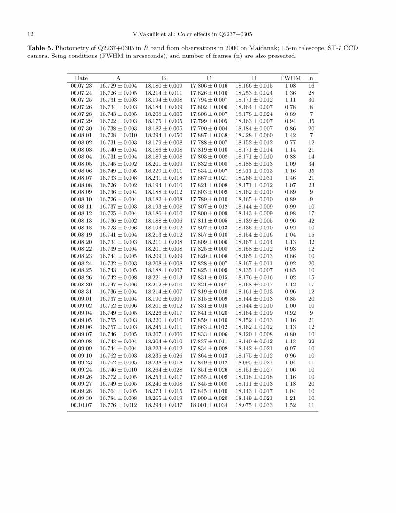
Table 5. Photometry of Q2237+0305 in R band from observations in 2000 on Maidanak; 1.5-m telescope, ST-7 CCDcamera. Seing conditions (FWHM in arcseconds), and number of frames (n) are also presented.

Date A B C D FWHM n

00.07.23 16.729 ± 0.004 18.180 ± 0.009 17.806 ± 0.016 18.166 ± 0.015 1.08 1600.07.24 16.726 ± 0.005 18.214 ± 0.011 17.826 ± 0.016 18.253 ± 0.024 1.36 2800.07.25 16.731 ± 0.003 18.194 ± 0.008 17.794 ± 0.007 18.171 ± 0.012 1.11 3000.07.26 16.734 ± 0.003 18.184 ± 0.009 17.802 ± 0.006 18.164 ± 0.007 0.78 800.07.28 16.743 ± 0.005 18.208 ± 0.005 17.808 ± 0.007 18.178 ± 0.024 0.89 700.07.29 16.722 ± 0.003 18.175 ± 0.005 17.799 ± 0.005 18.163 ± 0.007 0.94 3500.07.30 16.738 ± 0.003 18.182 ± 0.005 17.790 ± 0.004 18.184 ± 0.007 0.86 2000.08.01 16.728 ± 0.010 18.294 ± 0.050 17.887 ± 0.038 18.328 ± 0.060 1.42 700.08.02 16.731 ± 0.003 18.179 ± 0.008 17.788 ± 0.007 18.152 ± 0.012 0.77 1200.08.03 16.740 ± 0.004 18.186 ± 0.008 17.819 ± 0.010 18.171 ± 0.014 1.14 2100.08.04 16.731 ± 0.004 18.189 ± 0.008 17.803 ± 0.008 18.171 ± 0.010 0.88 1400.08.05 16.745 ± 0.002 18.201 ± 0.009 17.832 ± 0.008 18.188 ± 0.013 1.09 3400.08.06 16.749 ± 0.005 18.229 ± 0.011 17.834 ± 0.007 18.211 ± 0.013 1.16 3500.08.07 16.733 ± 0.008 18.231 ± 0.018 17.867 ± 0.021 18.266 ± 0.031 1.46 2100.08.08 16.726 ± 0.002 18.194 ± 0.010 17.821 ± 0.008 18.171 ± 0.012 1.07 2300.08.09 16.736 ± 0.004 18.188 ± 0.012 17.803 ± 0.009 18.162 ± 0.010 0.89 900.08.10 16.726 ± 0.004 18.182 ± 0.008 17.789 ± 0.010 18.165 ± 0.010 0.89 900.08.11 16.737 ± 0.003 18.193 ± 0.008 17.807 ± 0.012 18.144 ± 0.009 0.99 1000.08.12 16.725 ± 0.004 18.186 ± 0.010 17.800 ± 0.009 18.143 ± 0.009 0.98 1700.08.13 16.736 ± 0.002 18.188 ± 0.006 17.811 ± 0.005 18.139 ± 0.005 0.96 4200.08.18 16.723 ± 0.006 18.194 ± 0.012 17.807 ± 0.013 18.136 ± 0.010 0.92 1000.08.19 16.741 ± 0.004 18.213 ± 0.012 17.857 ± 0.010 18.154 ± 0.016 1.04 1500.08.20 16.734 ± 0.003 18.211 ± 0.008 17.809 ± 0.006 18.167 ± 0.014 1.13 3200.08.22 16.739 ± 0.004 18.201 ± 0.008 17.825 ± 0.008 18.158 ± 0.012 0.93 1200.08.23 16.744 ± 0.005 18.209 ± 0.009 17.820 ± 0.008 18.165 ± 0.013 0.86 1000.08.24 16.732 ± 0.003 18.208 ± 0.008 17.828 ± 0.007 18.167 ± 0.011 0.92 2000.08.25 16.743 ± 0.005 18.188 ± 0.007 17.825 ± 0.009 18.135 ± 0.007 0.85 1000.08.26 16.742 ± 0.008 18.221 ± 0.013 17.831 ± 0.015 18.176 ± 0.016 1.02 1500.08.30 16.747 ± 0.006 18.212 ± 0.010 17.821 ± 0.007 18.168 ± 0.017 1.12 1700.08.31 16.736 ± 0.004 18.214 ± 0.007 17.819 ± 0.010 18.161 ± 0.013 0.96 1200.09.01 16.737 ± 0.004 18.190 ± 0.009 17.815 ± 0.009 18.144 ± 0.013 0.85 2000.09.02 16.752 ± 0.006 18.201 ± 0.012 17.831 ± 0.010 18.144 ± 0.010 1.00 1000.09.04 16.749 ± 0.005 18.226 ± 0.017 17.841 ± 0.020 18.164 ± 0.019 0.92 900.09.05 16.755 ± 0.003 18.220 ± 0.010 17.859 ± 0.010 18.152 ± 0.013 1.16 2100.09.06 16.757 ± 0.003 18.245 ± 0.011 17.863 ± 0.012 18.162 ± 0.012 1.13 1200.09.07 16.746 ± 0.005 18.207 ± 0.006 17.833 ± 0.006 18.120 ± 0.008 0.80 1000.09.08 16.743 ± 0.004 18.204 ± 0.010 17.837 ± 0.011 18.140 ± 0.012 1.13 2200.09.09 16.744 ± 0.004 18.223 ± 0.012 17.834 ± 0.008 18.142 ± 0.021 0.97 1000.09.10 16.762 ± 0.003 18.235 ± 0.026 17.864 ± 0.013 18.175 ± 0.012 0.96 1000.09.23 16.762 ± 0.005 18.238 ± 0.018 17.849 ± 0.012 18.095 ± 0.027 1.04 1100.09.24 16.746 ± 0.010 18.264 ± 0.028 17.851 ± 0.026 18.151 ± 0.027 1.06 1000.09.26 16.772 ± 0.005 18.253 ± 0.017 17.855 ± 0.009 18.118 ± 0.018 1.16 1000.09.27 16.749 ± 0.005 18.240 ± 0.008 17.845 ± 0.008 18.111 ± 0.013 1.18 2000.09.28 16.764 ± 0.005 18.273 ± 0.015 17.845 ± 0.010 18.143 ± 0.017 1.04 1000.09.30 16.784 ± 0.008 18.265 ± 0.019 17.909 ± 0.020 18.149 ± 0.021 1.21 1000.10.07 16.776 ± 0.012 18.294 ± 0.037 18.001 ± 0.034 18.075 ± 0.033 1.52 11


Table 6. V RI Photometry of Q2237+0305 in 1995-2000; Maidanak, 1.5-m telescope.

Date A B C D Sp.band

17.34 ± 0.04 17.44 ± 0.03 18.41 ± 0.10 18.66 ± 0.08 V95.09.17 17.18 ± 0.03 17.32 ± 0.03 18.13 ± 0.06 18.44 ± 0.07 R

16.99 ± 0.03 17.21 ± 0.04 17.83 ± 0.08 18.23 ± 0.09 I

17.43 ± 0.03 17.95 ± 0.05 18.42 ± 0.05 18.78 ± 0.07 V97.08.29 17.15 ± 0.03 17.72 ± 0.03 18.08 ± 0.12 18.38 ± 0.10 R

16.96 ± 0.03 17.60 ± 0.04 17.81 ± 0.04 18.15 ± 0.07 I

17.40 ± 0.03 17.94 ± 0.04 18.35 ± 0.05 18.79 ± 0.06 V97.08.30 17.14 ± 0.02 17.75 ± 0.03 18.08 ± 0.04 18.41 ± 0.05 R

16.89 ± 0.02 17.55 ± 0.04 17.82 ± 0.03 18.11 ± 0.06 I

17.47 ± 0.05 18.01 ± 0.07 18.38 ± 0.06 18.91 ± 0.09 V97.09.01 17.13 ± 0.04 17.75 ± 0.05 18.01 ± 0.04 18.44 ± 0.11 R

16.93 ± 0.03 17.61 ± 0.04 17.83 ± 0.04 18.19 ± 0.09 I

17.30 ± 0.02 18.11 ± 0.05 17.66 ± 0.05 18.52 ± 0.05 V98.07.26 17.08 ± 0.04 17.82 ± 0.04 17.43 ± 0.06 18.12 ± 0.07 R

16.92 ± 0.03 17.71 ± 0.04 17.32 ± 0.04 17.87 ± 0.06 I

17.44 ± 0.03 18.23 ± 0.03 17.78 ± 0.03 18.64 ± 0.05 V98.07.28 17.14 ± 0.02 18.00 ± 0.02 17.63 ± 0.06 18.32 ± 0.12 R

16.93 ± 0.04 17.72 ± 0.05 17.47 ± 0.05 17.82 ± 0.06 I

17.52 ± 0.02 18.23 ± 0.02 17.77 ± 0.04 18.84 ± 0.07 V98.08.23 17.22 ± 0.07 18.03 ± 0.04 17.41 ± 0.03 18.33 ± 0.06 R

17.09 ± 0.04 17.83 ± 0.03 17.36 ± 0.04 18.14 ± 0.20 I

17.34 ± 0.05 18.28 ± 0.05 17.65 ± 0.06 18.48 ± 0.11 V98.11.14 17.07 ± 0.05 17.89 ± 0.06 17.43 ± 0.05 18.07 ± 0.08 R

16.94 ± 0.03 17.79 ± 0.05 17.44 ± 0.03 17.92 ± 0.06 I

16.89 ± 0.04 18.12 ± 0.05 17.19 ± 0.03 18.34 ± 0.11 V99.07.20 16.75 ± 0.06 17.99 ± 0.06 17.14 ± 0.04 18.15 ± 0.11 R

16.62 ± 0.02 17.76 ± 0.05 17.07 ± 0.02 17.84 ± 0.04 I

16.92 ± 0.02 18.16 ± 0.03 17.22 ± 0.02 18.40 ± 0.08 V99.07.22 16.78 ± 0.01 18.00 ± 0.03 17.13 ± 0.02 18.09 ± 0.02 R

16.63 ± 0.01 17.79 ± 0.03 17.09 ± 0.02 17.82 ± 0.03 I

16.888 ± 0.005 18.401 ± 0.016 18.011 ± 0.008 18.400 ± 0.007 V00.07.26 16.734 ± 0.003 18.184 ± 0.009 17.802 ± 0.006 18.164 ± 0.007 R

16.577 ± 0.004 17.973 ± 0.007 17.590 ± 0.008 17.911 ± 0.006 I

16.880 ± 0.004 18.387 ± 0.015 17.992 ± 0.011 18.392 ± 0.017 V00.08.04 16.731 ± 0.004 18.189 ± 0.008 17.803 ± 0.008 18.171 ± 0.010 R

16.577 ± 0.004 17.968 ± 0.007 17.604 ± 0.006 17.919 ± 0.004 I

16.894 ± 0.008 18.423 ± 0.010 18.032 ± 0.017 18.381 ± 0.020 V00.08.09 16.736 ± 0.004 18.188 ± 0.012 17.803 ± 0.009 18.162 ± 0.010 R

16.586 ± 0.005 17.976 ± 0.008 17.616 ± 0.010 17.925 ± 0.016 I

16.878 ± 0.008 18.365 ± 0.025 18.021 ± 0.030 18.350 ± 0.025 V00.08.18 16.723 ± 0.006 18.194 ± 0.012 17.807 ± 0.013 18.136 ± 0.010 R

16.574 ± 0.006 17.975 ± 0.010 17.612 ± 0.013 17.899 ± 0.012 I

16.882 ± 0.006 18.369 ± 0.014 18.008 ± 0.010 18.370 ± 0.015 V00.08.25 16.743 ± 0.005 18.188 ± 0.007 17.825 ± 0.009 18.135 ± 0.007 R

16.578 ± 0.003 17.982 ± 0.008 17.616 ± 0.004 17.884 ± 0.011 I

16.886 ± 0.006 18.398 ± 0.013 17.997 ± 0.007 18.328 ± 0.016 V00.09.07 16.746 ± 0.005 18.207 ± 0.006 17.833 ± 0.006 18.120 ± 0.008 R

16.583 ± 0.006 17.988 ± 0.010 17.612 ± 0.008 17.884 ± 0.012 I

16.918 ± 0.005 18.443 ± 0.011 18.057 ± 0.013 18.365 ± 0.016 V00.09.28 16.764 ± 0.005 18.273 ± 0.015 17.845 ± 0.010 18.143 ± 0.017 R

16.600 ± 0.006 18.006 ± 0.013 17.657 ± 0.006 17.871 ± 0.016 I


Table 7. (V − R) and (R− I) colors of Q2237+0305 A,B,C,D; 1995-2000, Maidanak, 1.5-m telescope.

Date A B C D

V-R V-I V-R V-I V-R V-I V-R V-I

17.09.95 0.16 0.35 0.12 0.23 0.28 0.42 0.22 0.5728.08.97 0.28 0.47 0.23 0.35 0.34 0.51 0.40 0.6330.08.97 0.26 0.51 0.19 0.39 0.27 0.63 0.38 0.6801.09.97 0.34 0.54 0.26 0.40 0.37 0.55 0.47 0.7226.07.98 0.22 0.38 0.29 0.40 0.23 0.34 0.40 0.6528.07.98 0.30 0.51 0.23 0.51 0.15 0.31 0.32 0.7023.08.98 0.30 0.43 0.20 0.60 0.36 0.41 0.51 0.7014.11.98 0.27 0.40 0.39 0.59 0.22 0.21 0.41 0.5620.07.99 0.14 0.27 0.13 0.34 0.05 0.12 0.19 0.5022.07.99 0.14 0.29 0.16 0.37 0.09 0.13 0.31 0.5826.07.00 0.15 0.31 0.22 0.43 0.21 0.42 0.24 0.4904.08.00 0.15 0.30 0.20 0.42 0.19 0.39 0.22 0.4709.08.00 0.15 0.31 0.23 0.45 0.23 0.42 0.22 0.4618.08.00 0.15 0.30 0.17 0.39 0.21 0.41 0.21 0.4525.08.00 0.14 0.30 0.18 0.39 0.18 0.39 0.23 0.4907.09.00 0.14 0.30 0.19 0.41 0.16 0.38 0.22 0.4428.09.00 0.15 0.32 0.17 0.44 0.21 0.40 0.22 0.39

This figure "0104_f1.gif" is available in "gif" format from:

http://arxiv.org/ps/astro-ph/0312631v1


1 , V.V.Konichek , I.Ye.Sinelnikov , O.M.Burkhonov , B.P ...

Documents

Transcript of 1 , V.V.Konichek , I.Ye.Sinelnikov , O.M.Burkhonov , B.P ...