1 Volume Fractions of Texture Components A. D. Rollett 27-750 Texture, Microstructure & Anisotropy...

1

Volume Fractions of Texture Components

A. D. Rollett

27-750 Texture, Microstructure & Anisotropy

Last revised: 4th Oct. ‘11

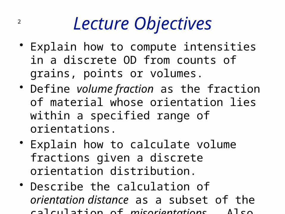
2 Lecture Objectives• Explain how to compute intensities in a discrete

OD from counts of grains, points or volumes.• Define volume fraction as the fraction of

material whose orientation lies within a specified range of orientations.

• Explain how to calculate volume fractions given a discrete orientation distribution.

• Describe the calculation of orientation distance as a subset of the calculation of misorientations. Also discuss how to apply symmetry, and some of the pitfalls.

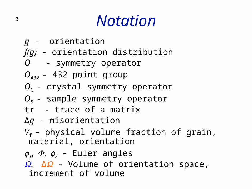
3 Notation g - orientation f(g) - orientation distribution O - symmetry operator

O432 - 432 point group

OC - crystal symmetry operator

OS - sample symmetry operator tr - trace of a matrix ∆g - misorientation

Vf – physical volume fraction of grain, material, orientation

- Euler angles ∆ - Volume of orientation space, increment of volume

In Class Questions

• How do we compute intensities from volume fractions?

• What is the difference between cell-edge and cell-centered coordinates?

• What do we mean by the volume fraction of a texture component?

• How do we compute the volume fraction of a component?

• What is a capture angle or tolerance angle or capture radius?

• What is a partition map?

• Why is the density of randomly chosen orientations (in Euler space) not uniform?

• Describe two ways to compute orientation distance.

• Why is misorientation useful for computing orientation distance?

• How do we apply symmetry to compute misorientation?

• Why do different components (e.g. cube vs. S) have different volume fractions in a random texture?

4

5

Intensity from Volume Fractions

Objective: given information on volume fractions (e.g. numbers of grains of a given orientation), how do we calculate the intensity in the OD? • General relationships:

€

V f (g) = f (g)dg∫

f (g) =1

V

dV (g)

dg=

ΔV f

ΔΩg

Reminder on units of the OD: the way that normalization is performed means that the units of the OD are Multiples of a Random Density (MRD). If there is no texture or preferred orientation then the value of “f” is one everywhere.

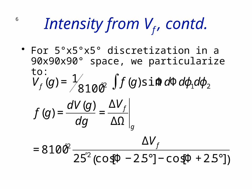
6 Intensity from Vf , contd.

• For 5°x5°x5° discretization in a 90x90x90° space, we particularize to:

€

V f (g) = 18100°2 f (g)sinΦdΦdϕ1dϕ 2∫

f (g) =dV (g)

dg=

ΔV f

ΔΩg

= 8100°2ΔV f

25°2 cos Φ − 2.5°[ ] − cos Φ + 2.5°[ ]( )

7

Discrete OD

• Normalization also required for discrete OD

• Sum the intensities over all the cells.• 0f1 2π, 0F π, 0f2 2π

0f1 90°, 0F 90°, 0f2 90°

1=1

8π2 f φ1,Φi ,φ2( )φ2

∑Φ∑

φ1

∑ Δφ1Δφ2 cosΦi −ΔΦ2

⎛ ⎝

⎞ ⎠ −cosΦi +

ΔΦ2

⎛ ⎝

⎞ ⎠

⎛ ⎝ ⎜

⎞ ⎠ ⎟

1=1

8100f φ1,Φi ,φ2( )

φ2

∑Φ∑

φ1

∑ Δφ1Δφ2 cosΦi −ΔΦ2

⎛ ⎝

⎞ ⎠ −cosΦi +

ΔΦ2

⎛ ⎝

⎞ ⎠

⎛ ⎝ ⎜

⎞ ⎠ ⎟

8

Volume fraction calculations

• Choice of cell size determines size of the volume increment, which depends on the value of the second angle (F or Q).

• Some grids start at the specified value.• More typical for the specified value to

be in the center of the cell.• popLA: grids are cell-centered.

9 Discrete ODs

0° 10° 20° 90°

90°

80°

80°

10°

20°

0°

∆ =10°F

f1

F

∆ f1 =10°

dA=sinFdFdf1:∆A=∆(cos )F ∆f1

Section at f2= 30°

∆f2=10°

f(10,10,30)

f(10,0,30)

f(10,80,30)

Each layer: ∆ W = S∆A∆f2 = 90(°)

Total: =W

8100(°)2

Cell edge discretization

10 Centered Cells

0° 10° 20° 90°

90°

80°

10°

20°

0°

∆ =10°F

f1

F

∆ f1 =10°

dA=sinFdFdf1:∆A=∆(cos )F ∆f1

….∆ =5°F

∆ f1 =5°

Different treatment of end and corner cells to exclude volume outside the subspace

f(10,10,30)

f(10,0,30)

f(10,90,30)

Cell centered discretization

11 Discrete orientation information

# WorkDirectory /usr/OIM/rollett# OIMDirectory /usr/OIM………...# 4.724 0.234 4.904 0.500 0.866 1.0 1.000 0 0 4.491 0.024 5.132 7.500 0.866 1.0 1.000 0 0 4.932 0.040 4.698 19.500 0.866 1.0 1.000 0 0 4.491 0.024 5.132 20.500 0.866 1.0 1.000 0 0 4.491 0.024 5.132 21.500 0.866 1.0 1.000 0 0 4.932 0.040 4.698 22.500 0.866 1.0 1.000 0 0 4.932 0.040 4.698 23.500 0.866 1.0 1.000 0 0 4.932 0.040 4.698 24.500 0.866 1.0 1.000 0 0

f1 F f2

(Euler angles, radians)

x y

Typical text data.ANG file from TSL EBSD system:

Each dataset may have millions of points

(spatial coordinates, microns)

12 Binning individual orientations in a discrete OD

0° 10° 20° 90°

90°

80°

80°

10°

20°

0°

∆ =10°F

f1

F

∆ f1 =10°

Section at f2= 30°

individualorientation

13 Example of random

orientation distribution in Euler spaceNote the smaller densities of points (arbitrary scale)

near F = 0°. When converted to intensities, however, then the result is a uniform, constant value of the OD (because of the effect of the volume element size, sindddf). If a material had randomly oriented grains all of the same size then this is how they would appear, as individual points in orientation space.

[Bunge]

14 OD from discrete points: pseudo-code

1. Compute the volume of the chosen orientation space, e.g. Euler space, e.g. 90° x 90° x 90° ⇒ W =∫dg = 8100 °2. Also compute the volume of each cell; in this case dW(f1, ,F f2) = ∆(cosF)∆f1∆f2

2. Bin each orientation into a cell in the OD

3. Sum number (or weight, if each orientation represents a different physical volume) in each cell

4. Divide the number (or physical volume) in each cell by the total number of grains (or total physical volume) to obtain Vf

5. Convert from Vf to f(g):

f(g) = 8100 Vf / {∆(cos )F ∆f1∆f2}

∆ W =cell volume W =∫dg

15 Discrete OD from points• The same Vf near F=0° will have much larger f(g)

than cells near F =90°.• Unless large number (>104, texture dependent) of

grains are measured, the resulting OD will be noisy, i.e. large variations in intensity between cells.

• Typically, smoothing is used to facilitate presentation of results: always do this last and as a visual aid only!

• An alternative to smoothing an ODF plot is to replace individual points by Gaussians and then evaluate the texture. This is particularly helpful (and commonly applied) when performing a series expansion fit to a set of individual orientation measurements, such as OIM data.

16

Volume fraction calculation

• In its simplest form: sum up the intensities multiplied by the value of the volume increment (invariant measure) for each cell.

• Check that when you compute this sum for the entire space the result is equal to one (else the normalization is not correct).

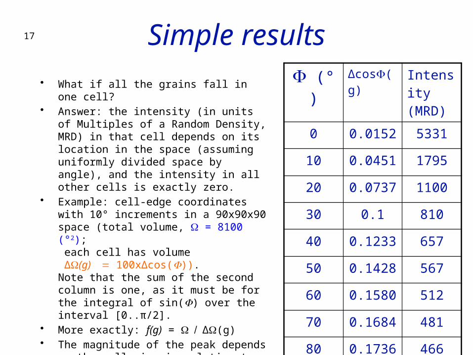
17 Simple results

• What if all the grains fall in one cell?• Answer: the intensity (in units of Multiples of

a Random Density, MRD) in that cell depends on its location in the space (assuming uniformly divided space by angle), and the intensity in all other cells is exactly zero.

• Example: cell-edge coordinates with 10° increments in a 90x90x90 space (total volume, = 8100 (°2); each cell has volume ∆(g) 100x∆cos()). Note that the sum of the second column is one, as it must be for the integral of sin() over the interval [0..π/2].

• More exactly: f(g) = ∆(g)• The magnitude of the peak depends on the

cell size in relation to the volume, not on the measure (degrees versus radians).

(°) ∆cos(g) Intensity (MRD)

0 0.0152 5331

10 0.0451 1795

20 0.0737 1100

30 0.1 810

40 0.1233 657

50 0.1428 567

60 0.1580 512

70 0.1684 481

80 0.1736 466

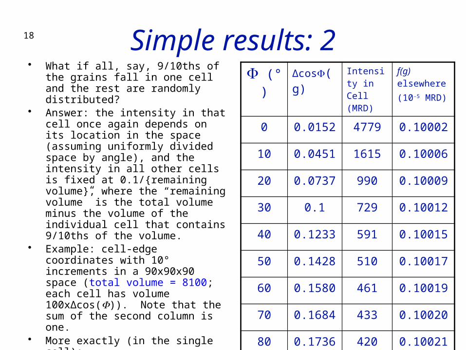
18 Simple results: 2• What if all, say, 9/10ths of the grains fall

in one cell and the rest are randomly distributed?

• Answer: the intensity in that cell once again depends on its location in the space (assuming uniformly divided space by angle), and the intensity in all other cells is fixed at 0.1/{remaining volume}, where the “remaining volume” is the total volume minus the volume of the individual cell that contains 9/10ths of the volume.

• Example: cell-edge coordinates with 10° increments in a 90x90x90 space (total volume = 8100; each cell has volume 100x∆cos()). Note that the sum of the second column is one.

• More exactly (in the single cell): f(g) = 0.9 ∆(g), - “peak”or elsewhere, since ∫f(g) = f(g) = 0.1 / (∆(g)) - “random”

(°) ∆cos(g) Intensity in Cell (MRD)

f(g) elsewhere(10-5 MRD)

0 0.0152 4779 0.10002

10 0.0451 1615 0.10006

20 0.0737 990 0.10009

30 0.1 729 0.10012

40 0.1233 591 0.10015

50 0.1428 510 0.10017

60 0.1580 461 0.10019

70 0.1684 433 0.10020

80 0.1736 420 0.10021

19

Acceptance Angle

• The simplest way to think about volume fractions is to consider that all cells within a certain angle of the location of the position of the texture component of interest belong to that component.

• Although we will need to use the concept of orientation distance (equivalent to misorientation), for now we can use a fixed angular distance or acceptance angle to decide which component a particular cell belongs to.

20

Acceptance Angle Schematic

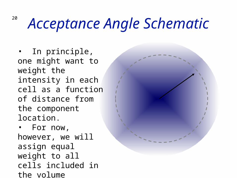
• In principle, one might want to weight the intensity in each cell as a function of distance from the component location.• For now, however, we will assign equal weight to all cells included in the volume fraction estimate.

21

Illustration of Acceptance Angle

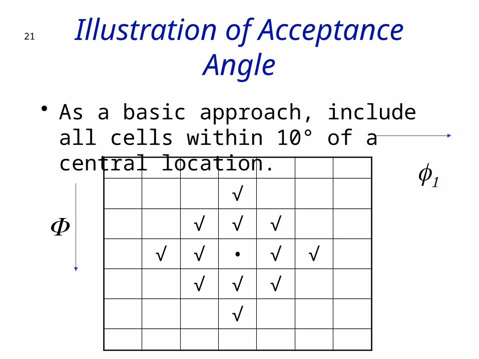
• As a basic approach, include all cells within 10° of a central location.

√√ √ √

√ √ • √ √√ √ √

√

F

f1

22 Copper component example

CUR80-2 6/13/88 35 Bwimv iter: 2.0%FON= 0 13-APR-** strength= 2.43 CODK 5.0 90.0 5.0 90.0 1 1 1 2 3 100 phi= 45.0 15 12 8 3 3 6 14 42 89 89 89 42 14 6 3 3 8 12 15 5 5 5 6 8 20 43 53 57 65 65 45 21 14 12 10 8 9 7 12 11 10 14 20 30 60 118 136 84 49 16 2 1 1 1 2 4 5 22 21 32 49 68 81 100 123 132 108 37 12 6 3 3 3 3 2 1 321 284 228 185 172 190 207 178 109 48 19 7 5 5 4 3 3 1 1 955 899 770 575 389 293 223 131 55 12 3 2 2 1 1 1 0 0 0 173015471100 652 382 233 132 62 23 7 2 1 1 1 1 0 1 0 0 15131342 881 436 191 90 53 29 17 6 2 1 0 0 1 0 0 0 0 137 135 109 77 59 41 24 10 4 2 1 0 0 0 0 0 0 0 0 1 0 1 3 5 10 13 14 10 3 1 1 0 0 0 0 0 0 0 0 1 1 1 1 1 1 1 1 0 0 0 0 0 0 0 0 0 0 0 0 0 1 1 1 1 1 1 1 0 0 0 0 0 1 1 1 1 0 0 0 0 1 0 1 2 2 1 1 1 2 2 3 4 5 6 7 0 0 0 0 1 1 2 4 5 5 5 4 3 6 8 6 6 7 5 2 2 2 2 2 2 2 2 4 3 3 3 4 7 9 6 12 17 16 3 4 4 4 4 7 33 80 86 66 42 29 29 31 33 40 51 46 40 7 7 9 14 31 71 144 179 145 81 31 11 7 7 10 17 25 23 23 203 190 188 193 224 304 417 486 410 249 109 51 36 26 16 12 12 12 8 301 315 404 559 752100511801140 861 494 237 132 65 42 29 26 31 30 30

15° acceptance angle; location of maximum intensity 5° off ideal position

F

f1

23

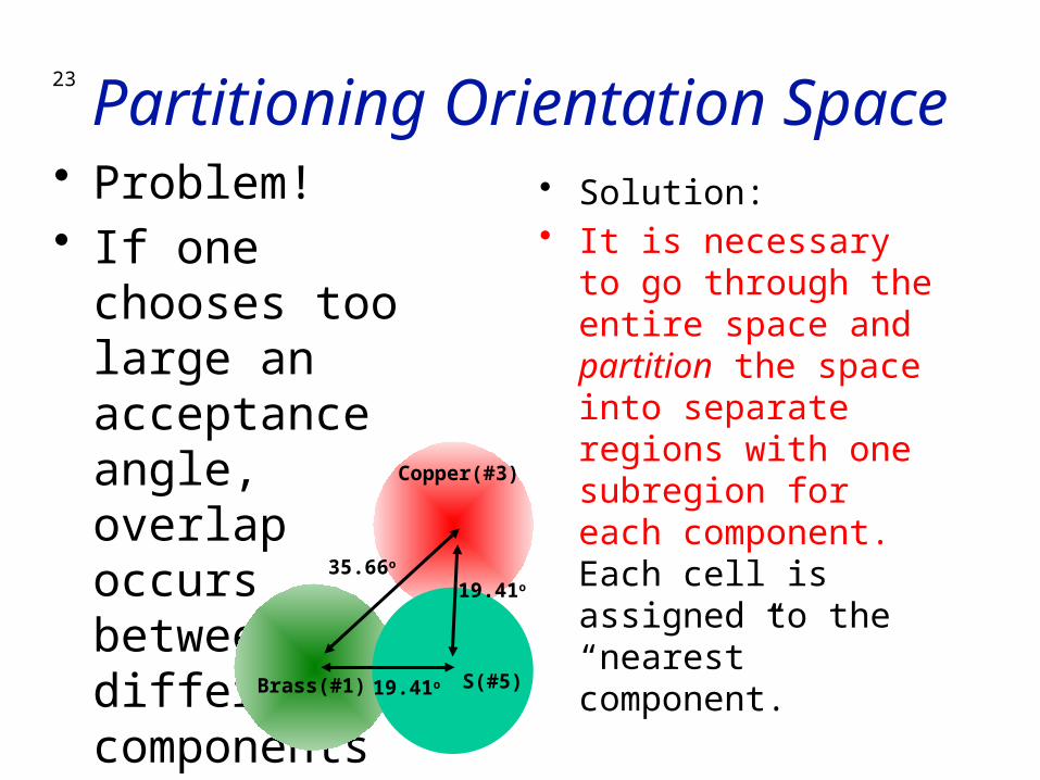
Partitioning Orientation Space• Problem!• If one chooses

too large an acceptance angle, overlap occurs between different components

• Solution:• It is necessary to go

through the entire space and partition the space into separate regions with one subregion for each component. Each cell is assigned to the “nearest” component.

Brass(#1)

Copper(#3)

35.66o

19.41o

S(#5)19.41o

24

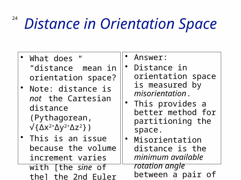
Distance in Orientation Space

• What does “distance” mean in orientation space?

• Note: distance is not the Cartesian distance (Pythagorean, √{∆x2+∆y2+∆z2})

• This is an issue because the volume increment varies with [the sine of the] the 2nd Euler angle.

• Answer:• Distance in orientation

space is measured by misorientation.

• This provides a better method for partitioning the space.

• Misorientation distance is the minimum available rotation angle between a pair of orientations.

25

Partitioning by Misorientation• Compute misorientation by “reversing” one orientation and then applying

the other orientation. More precisely stated, compose the inverse of one orientation with the other orientation.

• |∆g| = minij{ cos-1( { tr([OixtalgAOj

sample]gBT) -1}/2 )}

• The symbol “tr()” means the trace of (sum of leading diagonal entries) of the matrix within the parentheses. The minimum function indicates that one chooses the particular combination of crystal symmetry operator, OiO432, and sample symmetry operator, OjO222, that results in the smallest angle (for cubic crystals, computed for all 24 proper rotations in the crystal symmetry point group). Thus i=1..24 and j=1..4.

• Superscript T indicates (matrix) transpose which gives the inverse rotation. Subscripts A and B denote first and second component. For this purpose, the order of the rotations does not matter (but it will matter when the rotation axis is important!).

• Note that including the symmetry operators allows points near the edges of orientation space to be close to each other, even though they may be at opposite edges of the space.

• More details provided in later slides.

26 Partitioning by Misorientation, contd.

• For each point (cell) in the orientation space, compute the misorientation of that point with every component of interest (including all 3 variants of that component within the space); this gives a list of, say, six misorientation values between the cell and each of the six components of interest.

• Assign the point (cell) to the component with which it has the smallest misorientation, provided that it is less than the acceptance angle.

• If a point (cell) does not belong to a particular component (because it is not close enough), label it as “other” or “random”.

27 Partition Map, COD, f2 = 0° Acceptance angle (degrees) = 15.AL 3/08/02 99 WIMV iter: 1.2%,Fon= 0 20-MAY-** strength= 3.88 CODB 5.0 90.0 5.0 90.0 1 1 1 2 3 0 6859Phi2= 0.0 1 1 1 4 4 4 4 0 0 0 0 0 4 4 4 4 1 1 1 1 1 1 4 4 4 4 0 0 0 0 0 4 4 4 4 1 1 1 2 2 2 4 4 4 4 0 0 0 0 0 4 4 4 4 5 5 5 2 2 2 2 4 0 0 0 0 0 0 0 0 0 0 0 5 5 5 2 2 2 0 0 0 0 0 0 0 0 0 0 0 0 0 5 5 5 2 2 2 0 0 0 9 9 9 0 0 0 0 0 0 0 0 0 0 3 3 3 7 0 9 9 9 9 9 0 0 0 0 0 0 0 0 0 3 3 3 7 7 9 9 9 9 9 0 0 0 0 0 0 0 0 0 3 3 7 7 7 7 8 8 8 8 0 0 0 0 0 0 0 0 0 3 7 7 7 7 7 8 8 8 8 0 0 0 0 0 0 0 0 0 3 3 7 7 7 7 8 8 8 8 0 0 0 0 0 0 0 0 0 3 3 3 7 7 9 9 9 9 9 0 0 0 0 0 0 0 0 0 3 3 3 7 0 9 9 9 9 9 0 0 0 0 0 0 0 0 0 2 2 2 0 0 0 9 9 9 0 0 0 0 0 0 0 0 0 5 2 2 2 0 0 0 0 0 0 0 0 0 0 0 0 0 5 5 5 2 2 2 0 4 0 0 0 0 0 0 0 0 0 0 0 5 5 5 2 2 2 4 4 4 4 0 0 0 0 0 4 4 4 4 5 5 5 1 1 1 4 4 4 4 0 0 0 0 0 4 4 4 4 1 1 1 1 1 1 4 4 4 4 0 0 0 0 0 4 4 4 4 1 1 1

Cube Cube

Cube Cube

Brass

The number in each cell indicates which component it belongs to. 0 = “random”; 8 = Brass; 1 = Cube.

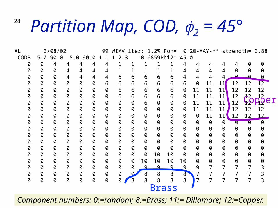
28 Partition Map, COD, f2 = 45°AL 3/08/02 99 WIMV iter: 1.2%,Fon= 0 20-MAY-** strength= 3.88 CODB 5.0 90.0 5.0 90.0 1 1 1 2 3 0 6859Phi2= 45.0 0 0 4 4 4 4 4 1 1 1 1 1 4 4 4 4 4 0 0 0 0 0 4 4 4 4 1 1 1 1 1 4 4 4 4 0 0 0 0 0 0 4 4 4 4 6 6 6 6 6 4 4 4 4 0 0 0 0 0 0 0 0 0 6 6 6 6 6 6 6 0 11 11 12 12 12 0 0 0 0 0 0 0 6 6 6 6 6 0 11 11 11 12 12 12 0 0 0 0 0 0 0 6 6 6 6 6 0 11 11 11 12 12 12 0 0 0 0 0 0 0 0 0 6 0 0 0 11 11 11 12 12 12 0 0 0 0 0 0 0 0 0 0 0 0 0 11 11 11 12 12 12 0 0 0 0 0 0 0 0 0 0 0 0 0 0 11 11 12 12 12 0 0 0 0 0 0 0 0 0 0 0 0 0 0 0 0 0 0 0 0 0 0 0 0 0 0 0 0 0 0 0 0 0 0 0 0 0 0 0 0 0 0 0 0 0 0 0 0 0 0 0 0 0 0 0 0 0 0 0 0 0 0 0 0 0 0 0 0 0 0 0 0 0 0 0 0 0 0 0 0 0 0 0 0 0 0 0 0 0 0 0 0 0 0 0 0 0 0 0 0 0 0 0 0 0 10 10 0 0 0 0 0 0 0 0 0 0 0 0 0 0 0 0 10 10 10 10 0 0 0 0 0 0 0 0 0 0 0 0 0 0 0 9 9 9 9 9 7 7 7 7 3 0 0 0 0 0 0 0 0 0 8 8 8 8 7 7 7 7 7 3 0 0 0 0 0 0 0 0 8 8 8 8 8 7 7 7 7 7 3

Brass

Copper

Component numbers: 0:=random; 8:=Brass; 11:= Dillamore; 12:=Copper.

29

Component Volumes: fcc

rolling texture• These contour

maps of individual components in Euler space are drawn for an acceptance angle of ~12°.

brass copper

S Goss

Cube

30

How to calculate misorientation?

• The next set of slides describe how to calculate misorientations, how to deal with crystal symmetry and sample symmetry, and some of the pitfalls that can arise.

• For orientation distance, only the magnitude of the difference in orientation needs to be calculated. Therefore some of the details that follow go beyond what you need for volume fraction. Nevertheless, you need to be aware of these issues so that you do not become confused in subsequent exercises.

• This misorientation calculation is not available in popLA but is available in TSL/HKL software. It is completely reliable but does not allow you to control the application of symmetry.

31

Objective

• To make clear how it is possible to express a misorientation in more than (physically) equivalent fashion.

• To allow researchers to apply symmetry correctly; mistakes are easy to make!

• It is essential to know how a rotation/orientation/texture component is expressed in order to know how to apply symmetry operations.

32

Worked Example• In this example, we take a pair of orientations that were chosen

to have a 60°<111> misorientation between them (rotation axis expressed in crystal coordinates). In fact the pair of orientations are the two sample symmetry related Copper components. The Copper component is nominally (112)[11-1].

• We calculate the 3x3 Rotation matrix for each orientation, gA

and gB, and then form the misorientation matrix, ∆g=gBgA-1.

• From the misorientation matrix, we calculate the angle, = cos-1(trace(∆g)-1)/2), and the rotation axis.

• In order to find the smallest possible misorientation angle, we have to apply crystal symmetry operators, O, to the misorientation matrix, O∆g, and recalculate the angle and axis.

• First, let’s examine the result….

33

Worked Example angles.. 90. 35.2599983 45. angles.. 270. 35.2599983 45.

1st Grain: Euler angles: 90. 35.2599983 45. 2nd Grain: Euler angles: 270. 35.2599983 45.

1st matrix:[ -0.577 0.707 0.408 ][ -0.577 -0.707 0.408 ][ 0.577 0.000 0.817 ]

2nd matrix:[ 0.577 -0.707 0.408 ][ 0.577 0.707 0.408 ][ -0.577 0.000 0.817 ]

Product matrix for gA X gB^-1:[ -0.667 0.333 0.667 ][ 0.333 -0.667 0.667 ][ 0.667 0.667 0.333 ] MISORI: angle= 60. axis= 1 1 -1

+

{100} pole figures

As it happens, the result is 60°[11-1], which looks reasonable, but is it, in fact, the smallest angle?

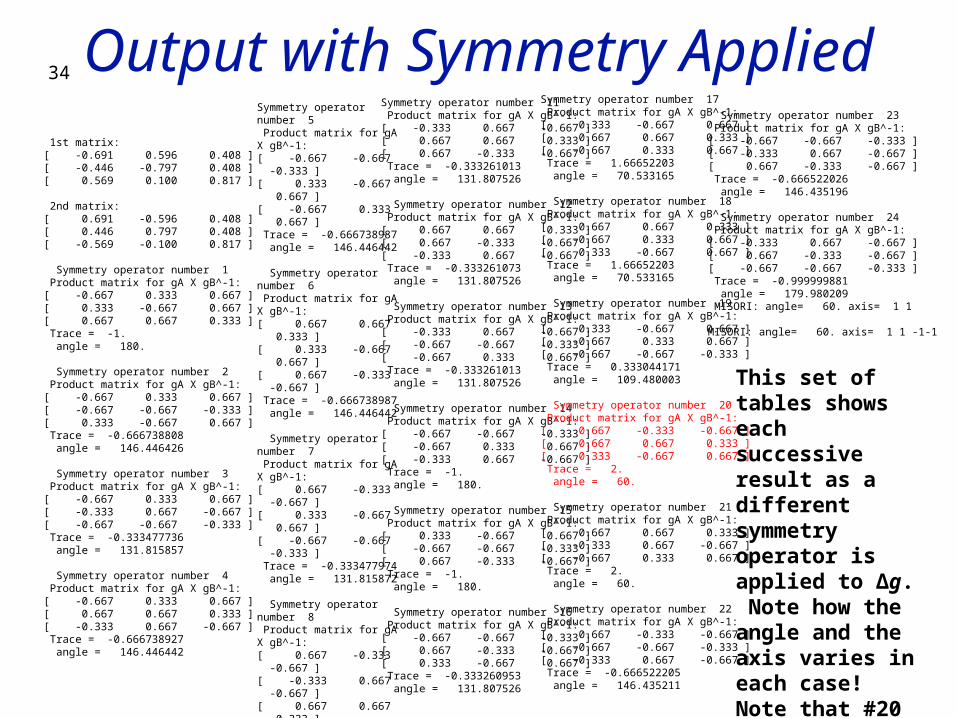
34 Output with Symmetry Applied 1st matrix:[ -0.691 0.596 0.408 ][ -0.446 -0.797 0.408 ][ 0.569 0.100 0.817 ]

2nd matrix:[ 0.691 -0.596 0.408 ][ 0.446 0.797 0.408 ][ -0.569 -0.100 0.817 ]

Symmetry operator number 1 Product matrix for gA X gB^-1:[ -0.667 0.333 0.667 ][ 0.333 -0.667 0.667 ][ 0.667 0.667 0.333 ] Trace = -1. angle = 180.

Symmetry operator number 2 Product matrix for gA X gB^-1:[ -0.667 0.333 0.667 ][ -0.667 -0.667 -0.333 ][ 0.333 -0.667 0.667 ] Trace = -0.666738808 angle = 146.446426

Symmetry operator number 3 Product matrix for gA X gB^-1:[ -0.667 0.333 0.667 ][ -0.333 0.667 -0.667 ][ -0.667 -0.667 -0.333 ] Trace = -0.333477736 angle = 131.815857

Symmetry operator number 4 Product matrix for gA X gB^-1:[ -0.667 0.333 0.667 ][ 0.667 0.667 0.333 ][ -0.333 0.667 -0.667 ] Trace = -0.666738927 angle = 146.446442

Symmetry operator number 5 Product matrix for gA X gB^-1:[ -0.667 -0.667 -0.333 ][ 0.333 -0.667 0.667 ][ -0.667 0.333 0.667 ] Trace = -0.666738987 angle = 146.446442

Symmetry operator number 6 Product matrix for gA X gB^-1:[ 0.667 0.667 0.333 ][ 0.333 -0.667 0.667 ][ 0.667 -0.333 -0.667 ] Trace = -0.666738987 angle = 146.446442

Symmetry operator number 7 Product matrix for gA X gB^-1:[ 0.667 -0.333 -0.667 ][ 0.333 -0.667 0.667 ][ -0.667 -0.667 -0.333 ] Trace = -0.333477974 angle = 131.815872

Symmetry operator number 8 Product matrix for gA X gB^-1:[ 0.667 -0.333 -0.667 ][ -0.333 0.667 -0.667 ][ 0.667 0.667 0.333 ] Trace = 1.66695571 angle = 70.5199966

Symmetry operator number 9 Product matrix for gA X gB^-1:[ 0.333 -0.667 0.667 ][ 0.667 -0.333 -0.667 ][ 0.667 0.667 0.333 ] Trace = 0.333477855 angle = 109.46682

Symmetry operator number 10 Product matrix for gA X gB^-1:[ -0.333 0.667 -0.667 ][ -0.667 0.333 0.667 ][ 0.667 0.667 0.333 ] Trace = 0.333477855 angle = 109.46682

Symmetry operator number 11 Product matrix for gA X gB^-1:[ -0.333 0.667 -0.667 ][ 0.667 0.667 0.333 ][ 0.667 -0.333 -0.667 ] Trace = -0.333261013 angle = 131.807526

Symmetry operator number 12 Product matrix for gA X gB^-1:[ 0.667 0.667 0.333 ][ 0.667 -0.333 -0.667 ][ -0.333 0.667 -0.667 ] Trace = -0.333261073 angle = 131.807526

Symmetry operator number 13 Product matrix for gA X gB^-1:[ -0.333 0.667 -0.667 ][ -0.667 -0.667 -0.333 ][ -0.667 0.333 0.667 ] Trace = -0.333261013 angle = 131.807526

Symmetry operator number 14 Product matrix for gA X gB^-1:[ -0.667 -0.667 -0.333 ][ -0.667 0.333 0.667 ][ -0.333 0.667 -0.667 ] Trace = -1. angle = 180.

Symmetry operator number 15 Product matrix for gA X gB^-1:[ 0.333 -0.667 0.667 ][ -0.667 -0.667 -0.333 ][ 0.667 -0.333 -0.667 ] Trace = -1. angle = 180.

Symmetry operator number 16 Product matrix for gA X gB^-1:[ -0.667 -0.667 -0.333 ][ 0.667 -0.333 -0.667 ][ 0.333 -0.667 0.667 ] Trace = -0.333260953 angle = 131.807526

Symmetry operator number 17 Product matrix for gA X gB^-1:[ 0.333 -0.667 0.667 ][ 0.667 0.667 0.333 ][ -0.667 0.333 0.667 ] Trace = 1.66652203 angle = 70.533165

Symmetry operator number 18 Product matrix for gA X gB^-1:[ 0.667 0.667 0.333 ][ -0.667 0.333 0.667 ][ 0.333 -0.667 0.667 ] Trace = 1.66652203 angle = 70.533165

Symmetry operator number 19 Product matrix for gA X gB^-1:[ 0.333 -0.667 0.667 ][ -0.667 0.333 0.667 ][ -0.667 -0.667 -0.333 ] Trace = 0.333044171 angle = 109.480003

Symmetry operator number 20 Product matrix for gA X gB^-1:[ 0.667 -0.333 -0.667 ][ 0.667 0.667 0.333 ][ 0.333 -0.667 0.667 ] Trace = 2. angle = 60.

Symmetry operator number 21 Product matrix for gA X gB^-1:[ 0.667 0.667 0.333 ][ -0.333 0.667 -0.667 ][ -0.667 0.333 0.667 ] Trace = 2. angle = 60.

Symmetry operator number 22 Product matrix for gA X gB^-1:[ 0.667 -0.333 -0.667 ][ -0.667 -0.667 -0.333 ][ -0.333 0.667 -0.667 ] Trace = -0.666522205 angle = 146.435211

Symmetry operator number 23 Product matrix for gA X gB^-1:[ -0.667 -0.667 -0.333 ][ -0.333 0.667 -0.667 ][ 0.667 -0.333 -0.667 ] Trace = -0.666522026 angle = 146.435196

Symmetry operator number 24 Product matrix for gA X gB^-1:[ -0.333 0.667 -0.667 ][ 0.667 -0.333 -0.667 ][ -0.667 -0.667 -0.333 ] Trace = -0.999999881 angle = 179.980209 MISORI: angle= 60. axis= 1 1

MISORI: angle= 60. axis= 1 1 -1-1

This set of tables shows each successive result as a different symmetry operator is applied to ∆g. Note how the angle and the axis varies in each case! Note that #20 is the one that gives a 60° angle.

35 Misorientations

• Misorientations:

∆g=gBgA-1

transform from crystal axes of grain A back to the reference axes, and then transform to the axes of grain B.

• Note that this use of “g” is based on the standard Bunge definition (transformation of axes)

36 Notation

• In some texts, misorientation formed from axis transformations is written with a tilde.

• Standard A->B transformation is expressed in crystal axes. The reason for this is that we generally want to know the common axis between the two crystals in terms of crystal coordinates.

Δ˜ g

37 Misorientation +Symmetry

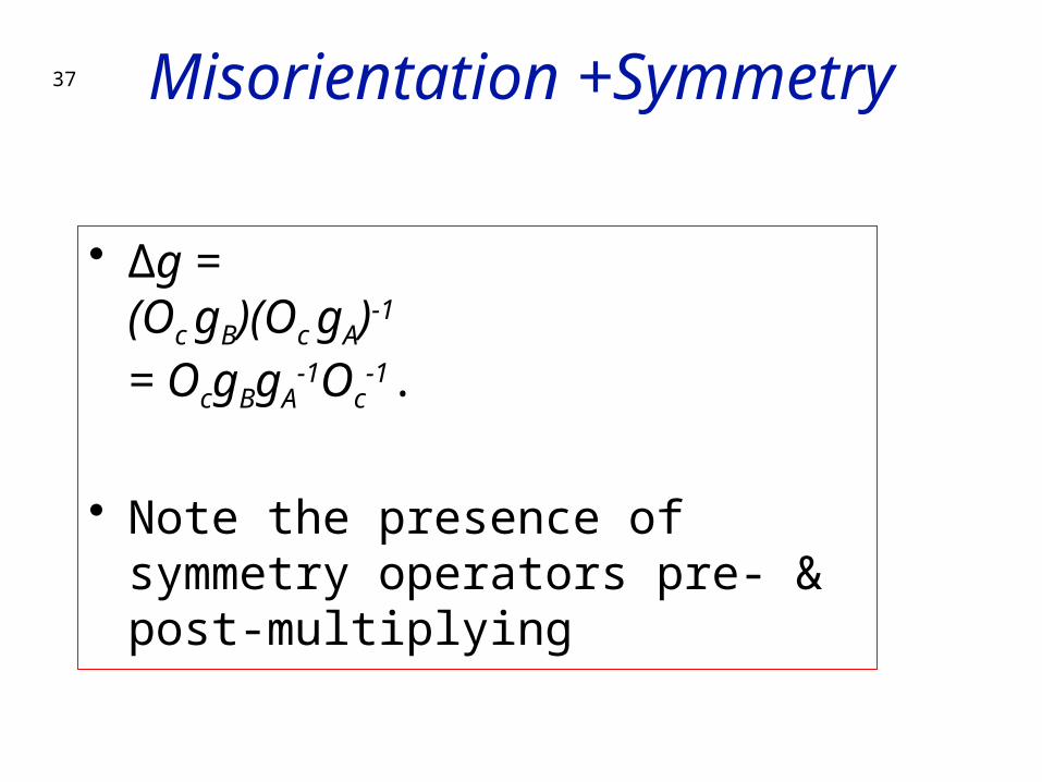
• ∆g =(Oc gB)(Oc gA)-1

= OcgBgA-1Oc

-1.

• Note the presence of symmetry operators pre- & post-multiplying

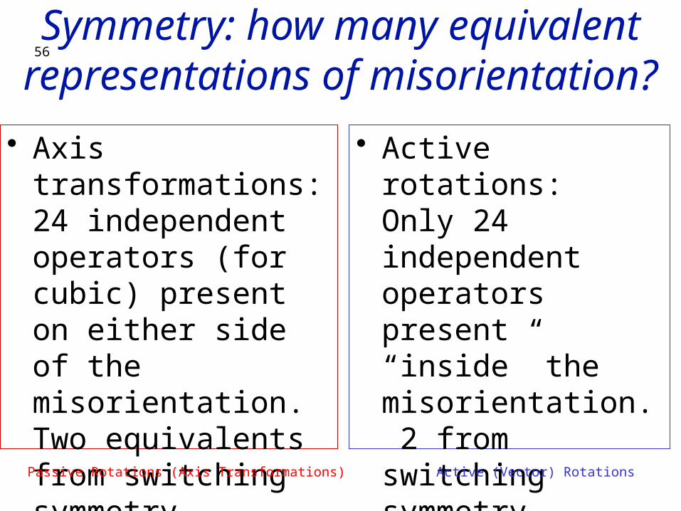
38Symmetry: how many equivalent

representations of misorientation?

• Axis transformations:24 independent operators (for cubic) present on either side of the misorientation. Two equivalents from switching symmetry, i.e. the fact that there is no (physical) difference between passing from grain A to grain B, versus passing from grain B to grain A.

• Number of equivalents = 24x24x2=1152.

39

When to include Sample Symmetry?

• The rule is simple:• For calculating orientation distances for the

purpose of partitioning orientation space, you do include sample symmetry. You only have to apply the sample symmetry, however, to either the component or the cell being tested but not both.

• For calculating misorientations for the purpose of characterizing grain boundaries, you do not include sample symmetry.

40

Practical Help with Volume Fractions

• To calculate volume fractions directly from popLA .SOD files (orientation distributions in popLA format), use sod2vf.f (a Fortran 77 code)

• To calculate volume fractions from a list of discrete orientations in .WTS format, use wts2pop[-latest_revision_date].f, which also bins the orientations into an SOD as well as pole figures and inverse pole figures. Look at any .WTS file to learn about the format (or read the popLA manual). You can find these programs at neon.materials.cmu.edu/rollett/texture_subroutines

• If your data source is a *.ANG orientation map (from TSL, or, a *.CTF from HKL) then first use OIM2WTS.f to convert it to the .WTS format. If your material has hexagonal symmetry be very careful about how the Cartesian x-axis is aligned with the crystal axes (TSL and HKL are, typically, different).

41

Volume fractions from Random?

• Based on a list of 20,000 random orientations and a 15° acceptance angle, you should expect this set of volume fractions:

• {001}<100> cube vol. frac.= 2.175 %{001}<110> NDcube vol. frac.= 2.144 %{011}<100> Goss vol. frac.= 2.310 %{110}<112> brass vol. frac.= 4.116 % Dillamore vol. frac.= 3.030 %{211}<111> Copper vol. frac.= 3.721 %{231}<124> S vol. frac.= 8.475 %

42 Volume fractions from Random?• Based on a list of 20,000 random orientations and a 10° acceptance

angle, you should expect this set of volume fractions:For component cube vol. frac.= 0.575 %For component NDcube vol. frac.= 0.690 %For component Goss vol. frac.= 0.715 %For component brass vol. frac.= 1.310 %For component Dillam vol. frac.= 1.103 %For component Copper vol. frac.= 1.382 %For component 231124 vol. frac.= 2.775 %

• Note how the volume fractions have decreased markedly with the decrease in acceptance angle.

• Eliminating the Dillamore component, which is only about 10° from Copper, the following set is found: note that Copper has increased but not by a factor of 2.For component cube vol. frac.= 0.575 %For component NDcube vol. frac.= 0.690 %For component Goss vol. frac.= 0.715 %For component brass vol. frac.= 1.310 %For component Copper vol. frac.= 1.710 %For component 231124 vol. frac.= 2.775 %

More Random/Uniform Volume Fractions by Component

Taken from unpublished work by Creuziger, Hu & Rollett (2010).

43

Variations in Random Vf• Why do the volume fractions vary with component

location?• Answer: mainly because of variations in how close

they lie to symmetry planes in orientation space.• Assume cubic-orthorhombic (crystal+sample)

symmetry• An orientation such as Goss lies on one edge, so

despite including 3 symmetry-related locations, its volume is only about 1/4th of, say, the S component.

• Similarly the Copper component, only includes 1/2th of the space of the S component.

• The rest of the variation is related to location with respect to the second Euler angle. See the next slide for illustrations of the above points.

44

45

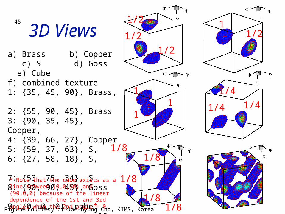
3D Viewsa) Brass b) Copper c) S d) Goss e) Cube f) combined texture 1: {35, 45, 90}, Brass, 2: {55, 90, 45}, Brass3: {90, 35, 45}, Copper, 4: {39, 66, 27}, Copper5: {59, 37, 63}, S, 6: {27, 58, 18}, S, 7: {53, 75, 34}, S 8: {90, 90, 45}, Goss 9: {0, 0, 0}, cube* 10: {45, 0, 0}, rotated cube* Note that the cube exists as a line between (0,0,90) and (90,0,0) because of the linear dependence of the 1st and 3rd angles when the 2nd angle = 0.

Figure courtesy of Jae-hyung Cho, KIMS, Korea

1/2

1/2

1/2

1/21

1

11 1/41/4

1/4

1/8

1/8

1/81/8

1/8

Scaling by Random Vf

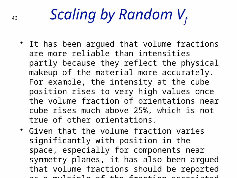
• It has been argued that volume fractions are more reliable than intensities partly because they reflect the physical makeup of the material more accurately. For example, the intensity at the cube position rises to very high values once the volume fraction of orientations near cube rises much above 25%, which is not true of other orientations.

• Given that the volume fraction varies significantly with position in the space, especially for components near symmetry planes, it has also been argued that volume fractions should be reported as a multiple of the fraction associated with a random (uniform) texture.

46

47

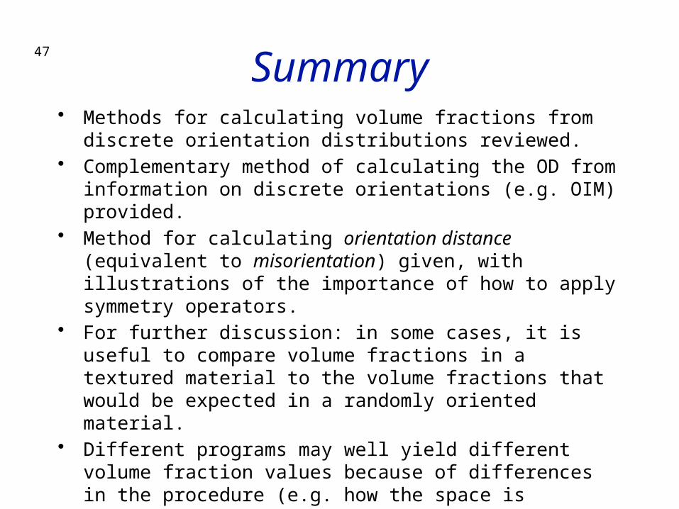
Summary• Methods for calculating volume fractions from discrete

orientation distributions reviewed.• Complementary method of calculating the OD from information

on discrete orientations (e.g. OIM) provided.• Method for calculating orientation distance (equivalent to

misorientation) given, with illustrations of the importance of how to apply symmetry operators.

• For further discussion: in some cases, it is useful to compare volume fractions in a textured material to the volume fractions that would be expected in a randomly oriented material.

• Different programs may well yield different volume fraction values because of differences in the procedure (e.g. how the space is partitioned).

48 Supplemental Slides• The following slides illustrate what happens with

misorientations if you deal with active rotations, instead of the standard axis transformations (passive rotations) used in materials science.

• This material is useful in case you have experience with solid mechanics, or you cannot get a misorientation calculation to work properly.

• Note: it does not matter whether you use passive or active rotations for computing the rotation angle; it only makes a difference to the rotation axis, i.e. the skew-symmetric part of the misorientation matrix.

49 Passive vs. Active Rotations

• Passive Rotations• Materials Science• g describes an axis transformation from

sample to crystal axes

• Active Rotations• Solid mechanics• g describes a rotation of a crystal from

ref. position to its orientation.

Passive Rotations (Axis Transformations) Active (Vector) Rotations

These next few slides describe the differences between dealing with passive rotations (= transformations of axes) and active rotations (fixed coordinate system)

50

Matricesg = Z2XZ1 =

g = gf1001gF100gf2001 =

cosϕ1cosϕ2

−sinϕ1sinϕ2cosΦ

sinϕ1cosϕ2

+cosϕ1sinϕ2cosΦsinϕ2sinΦ

−cosϕ1sinϕ2

−sinϕ1cosϕ2cosΦ

−sinϕ1sinϕ2

+cosϕ1cosϕ2cosΦ

cosϕ2sinΦ

sinϕ1sinΦ −cosϕ1sinΦ cosΦ

⎛

⎝

⎜ ⎜ ⎜ ⎜ ⎜ ⎜ ⎜ ⎜

⎞

⎠

⎟ ⎟ ⎟ ⎟ ⎟ ⎟ ⎟ ⎟

cosϕ1cosϕ2

−sinϕ1sinϕ2cosΦ

−cosϕ1sinϕ2

−sinϕ1cosϕ2cosΦsinϕ1sinΦ

sinϕ1cosϕ2

+cosϕ1sinϕ2cosΦ

−sinϕ1sinϕ2

+cosϕ1cosϕ2cosΦ

−cosϕ1sinΦ

sinϕ2sinΦ cosϕ2sinΦ cosΦ

⎛

⎝

⎜ ⎜ ⎜ ⎜ ⎜ ⎜ ⎜ ⎜ ⎜ ⎜

⎞

⎠

⎟ ⎟ ⎟ ⎟ ⎟ ⎟ ⎟ ⎟ ⎟ ⎟


Note transpose relationship between the two matrices.

51

Texture +SymmetrySymmetry Operators:

Osample Os

Ocrystal Oc

Note that the crystal symmetry post-multiplies, and the sample symmetry pre-multiplies.

Note the reversal in order of application of symmetry operators!

€

′ g = OcgOs

′ g =← → ⏐ g

€

′ g = OsgOc

′ g =← → ⏐ g


52

Groups: Sample +Crystal Symmetry

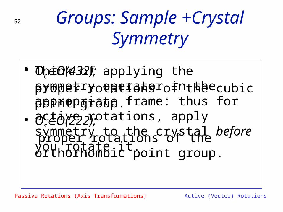
• OcO(432);proper rotations of the cubic point group.

• OsO(222); proper rotations of the orthorhombic point group.

• Think of applying the symmetry operator in the appropriate frame: thus for active rotations, apply symmetry to the crystal before you rotate it.


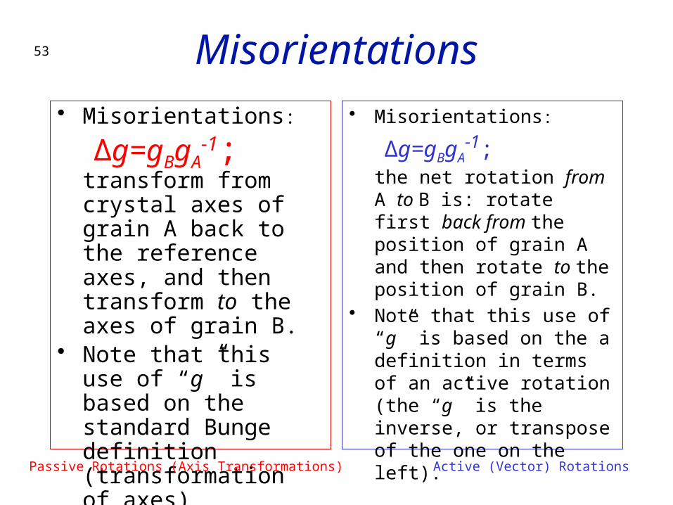
53 Misorientations• Misorientations:

∆g=gBgA-1;

transform from crystal axes of grain A back to the reference axes, and then transform to the axes of grain B.

• Note that this use of “g” is based on the standard Bunge definition (transformation of axes)

• Misorientations:

∆g=gBgA-1;

the net rotation from A to B is: rotate first back from the position of grain A and then rotate to the position of grain B.

• Note that this use of “g” is based on the a definition in terms of an active rotation (the “g” is the inverse, or transpose of the one on the left).


54 Notation

• In some texts, misorientation formed from axis transformations is written with a tilde.

• Standard A->B transformation is expressed in crystal axes.

• You must verify from the context which type of misorientation is discussed in a text!

• Standard A->B rotation is expressed in sample axes.

Δ˜ g


55 Misorientation +Symmetry

• ∆g=(Oc gB)(Oc gA)-1

= OcgBgA-1Oc

-1.

• Note the presence of symmetry operators pre- & post-multiplying

• ∆g=gBgA-1;

(gBOc)(gAOc)-1

= gBOcOc-1gA

-1

= gBOc’gA-1.

• Note the reduction to a single symmetry operator because the symmetry operators belong to the same group!


56Symmetry: how many equivalent

representations of misorientation?

• Axis transformations:24 independent operators (for cubic) present on either side of the misorientation. Two equivalents from switching symmetry.

• Number of equivalents=24x24x2=1152.

• Active rotations:Only 24 independent operators present “inside” the misorientation. 2 from switching symmetry.

• Number of equivalents=24x2=48.Passive Rotations (Axis Transformations) Active (Vector) Rotations

57

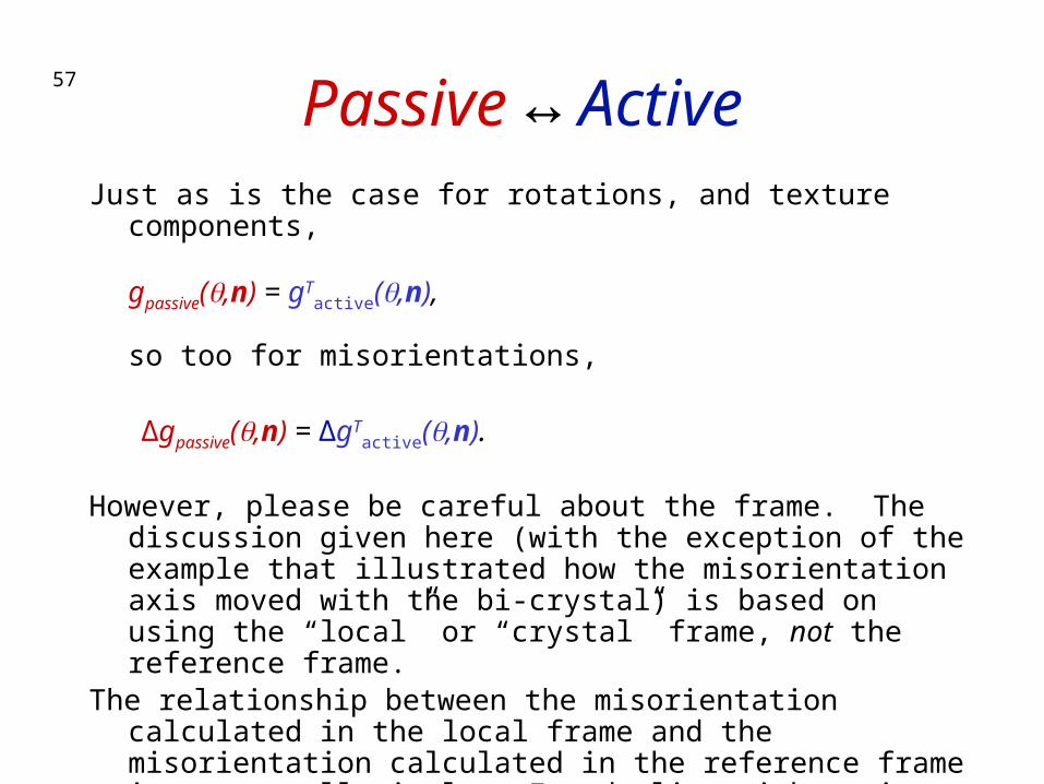
Passive ↔ ActiveJust as is the case for rotations, and texture components,

gpassive(q,n) = gTactive(q,n),

so too for misorientations,

∆gpassive(q,n) = ∆gTactive(q,n).

However, please be careful about the frame. The discussion given here (with the exception of the example that illustrated how the misorientation axis moved with the bi-crystal) is based on using the “local” or “crystal” frame, not the reference frame.

The relationship between the misorientation calculated in the local frame and the misorientation calculated in the reference frame is not at all simple. For dealing with grain boundaries, I strongly suggest that you stick to the local/crystal frame.

58

Worked example: active rotations• So what happens when we

express orientations as active rotations in the sample reference frame?

• The result is similar (same minimum rotation angle) but the axis is different!

• The rotation axis is the sample [100] axis, or x-axis, which happens to be parallel to a crystal <111> direction because the Copper component is (112)[11-1].

{100} pole figures

60° rotationabout RD

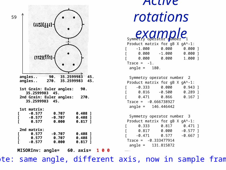
59Active rotations

example Symmetry operator number 1 Product matrix for gB X gA^-1:[ -1.000 0.000 0.000 ][ 0.000 -1.000 0.000 ][ 0.000 0.000 1.000 ] Trace = -1. angle = 180.

Symmetry operator number 2 Product matrix for gB X gA^-1:[ -0.333 0.000 0.943 ][ 0.816 -0.500 0.289 ][ 0.471 0.866 0.167 ] Trace = -0.666738927 angle = 146.446442

Symmetry operator number 3 Product matrix for gB X gA^-1:[ 0.333 0.817 0.471 ][ 0.817 0.000 -0.577 ][ -0.471 0.577 -0.667 ] Trace = -0.333477914 angle = 131.815872…………..

Note: same angle, different axis, now in sample frame

angles.. 90. 35.2599983 45. angles.. 270. 35.2599983 45.

1st Grain: Euler angles: 90. 35.2599983 45.

2nd Grain: Euler angles: 270. 35.2599983 45.

1st matrix:[ -0.577 0.707 0.408 ][ -0.577 -0.707 0.408 ][ 0.577 0.000 0.817 ]

2nd matrix:[ 0.577 -0.707 0.408 ][ 0.577 0.707 0.408 ][ -0.577 0.000 0.817 ]

MISORInv: angle= 60. axis= 1 0 0

60

Active rotations

• What is stranger, at first sight, is that, as you rotate the two orientations together in the sample frame, the misorientation axis moves with them, if expressed in the reference frame (active rotations).

• On the other hand, if one uses passive rotations, so that the result is in crystal coordinates, then the misorientation axis remains unchanged, as you rotate the pair of cr.

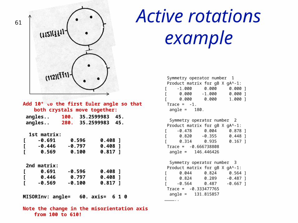
61 Active rotations example

Add 10° to the first Euler angle so that both crystals move together:

angles.. 100. 35.2599983 45. angles.. 280. 35.2599983 45.

1st matrix:[ -0.691 0.596 0.408 ][ -0.446 -0.797 0.408 ][ 0.569 0.100 0.817 ]

2nd matrix:[ 0.691 -0.596 0.408 ][ 0.446 0.797 0.408 ][ -0.569 -0.100 0.817 ]

MISORInv: angle= 60. axis= 6 1 0

Note the change in the misorientation axis from 100 to 610!

Symmetry operator number 1 Product matrix for gB X gA^-1:[ -1.000 0.000 0.000 ][ 0.000 -1.000 0.000 ][ 0.000 0.000 1.000 ] Trace = -1. angle = 180.

Symmetry operator number 2 Product matrix for gB X gA^-1:[ -0.478 0.004 0.878 ][ 0.820 -0.355 0.448 ][ 0.314 0.935 0.167 ] Trace = -0.666738808 angle = 146.446426

Symmetry operator number 3 Product matrix for gB X gA^-1:[ 0.044 0.824 0.564 ][ 0.824 0.289 -0.487 ][ -0.564 0.487 -0.667 ] Trace = -0.333477765 angle = 131.815857…………..

1 Volume Fractions of Texture Components A. D. Rollett 27-750 Texture, Microstructure & Anisotropy...

Documents

Transcript of 1 Volume Fractions of Texture Components A. D. Rollett 27-750 Texture, Microstructure & Anisotropy...