
1 -val_gillet_-_ligand-based_and_structure-based_virtual_screening
83
Ligand-Based and Structure-Based Virtual Screening Val Gillet University of Sheffield
-
Upload
deependra-ban -
Category
Engineering
-
view
100 -
download
0
Transcript of 1 -val_gillet_-_ligand-based_and_structure-based_virtual_screening

Ligand-Based and Structure-Based
Virtual Screening
Val Gillet University of Sheffield
Bio
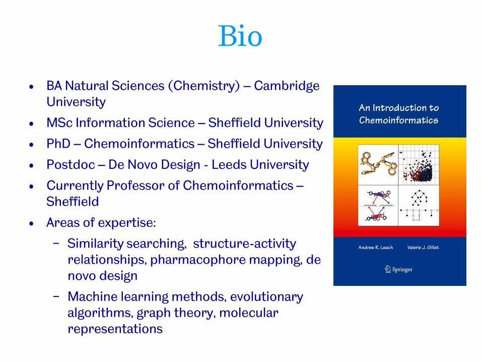
• BA Natural Sciences (Chemistry) – Cambridge University
• MSc Information Science – Sheffield University
• PhD – Chemoinformatics – Sheffield University
• Postdoc – De Novo Design - Leeds University
• Currently Professor of Chemoinformatics – Sheffield
• Areas of expertise:
− Similarity searching, structure-activity relationships, pharmacophore mapping, de novo design
− Machine learning methods, evolutionary algorithms, graph theory, molecular representations
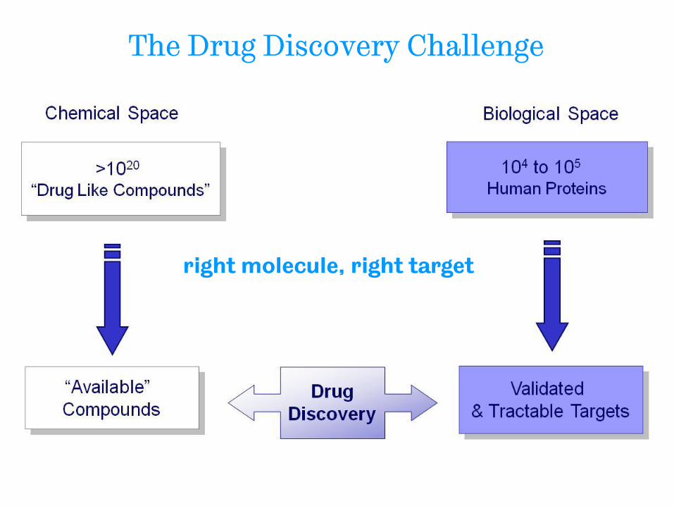
The Drug Discovery Challenge
right molecule, right target

High throughput automation High-throughput screening Combinatorial chemistry
Still need to consider carefully what to screen/make
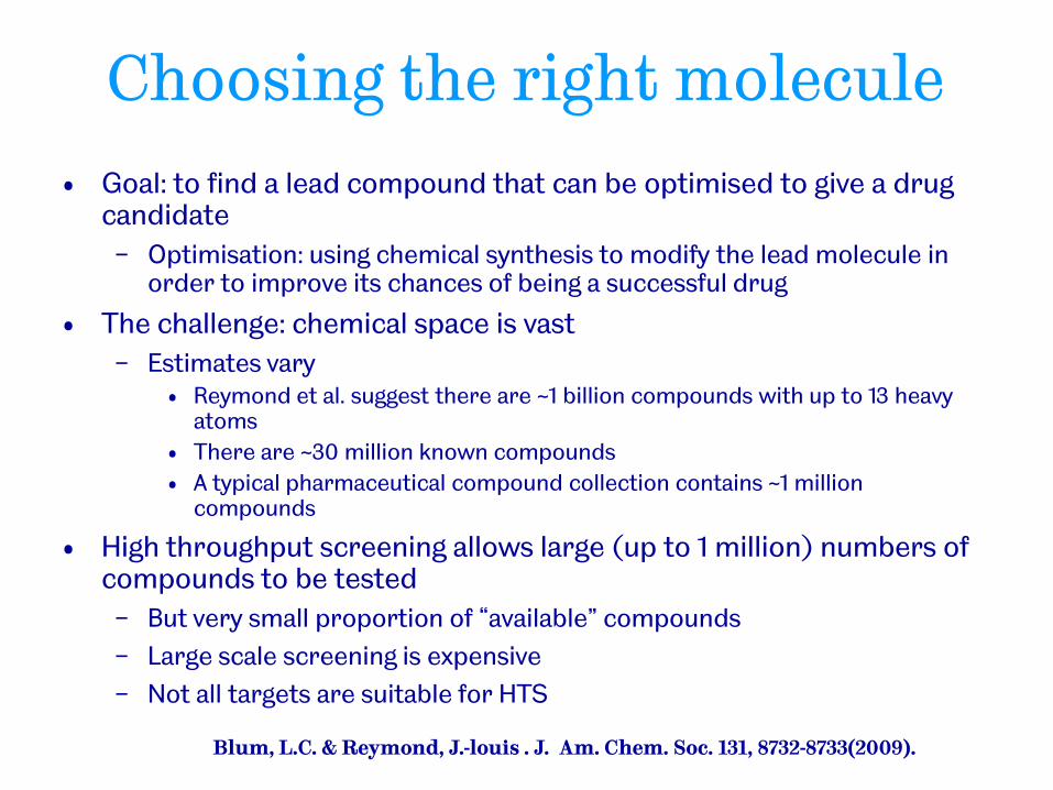
Choosing the right molecule
• Goal: to find a lead compound that can be optimised to give a drug candidate
− Optimisation: using chemical synthesis to modify the lead molecule in order to improve its chances of being a successful drug
• The challenge: chemical space is vast
− Estimates vary • Reymond et al. suggest there are ~1 billion compounds with up to 13 heavy
atoms
• There are ~30 million known compounds
• A typical pharmaceutical compound collection contains ~1 million compounds
• High throughput screening allows large (up to 1 million) numbers of compounds to be tested
− But very small proportion of “available” compounds
− Large scale screening is expensive
− Not all targets are suitable for HTS
Blum, L.C. & Reymond, J.-louis . J. Am. Chem. Soc. 131, 8732-8733(2009).
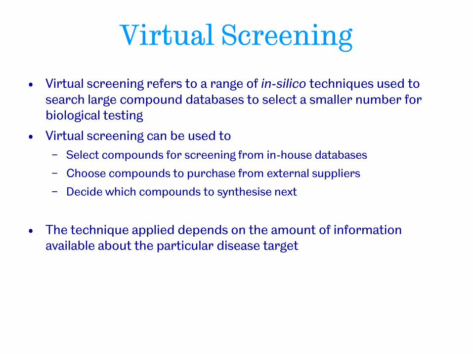
Virtual Screening
• Virtual screening refers to a range of in-silico techniques used to search large compound databases to select a smaller number for biological testing
• Virtual screening can be used to
− Select compounds for screening from in-house databases
− Choose compounds to purchase from external suppliers
− Decide which compounds to synthesise next
• The technique applied depends on the amount of information available about the particular disease target
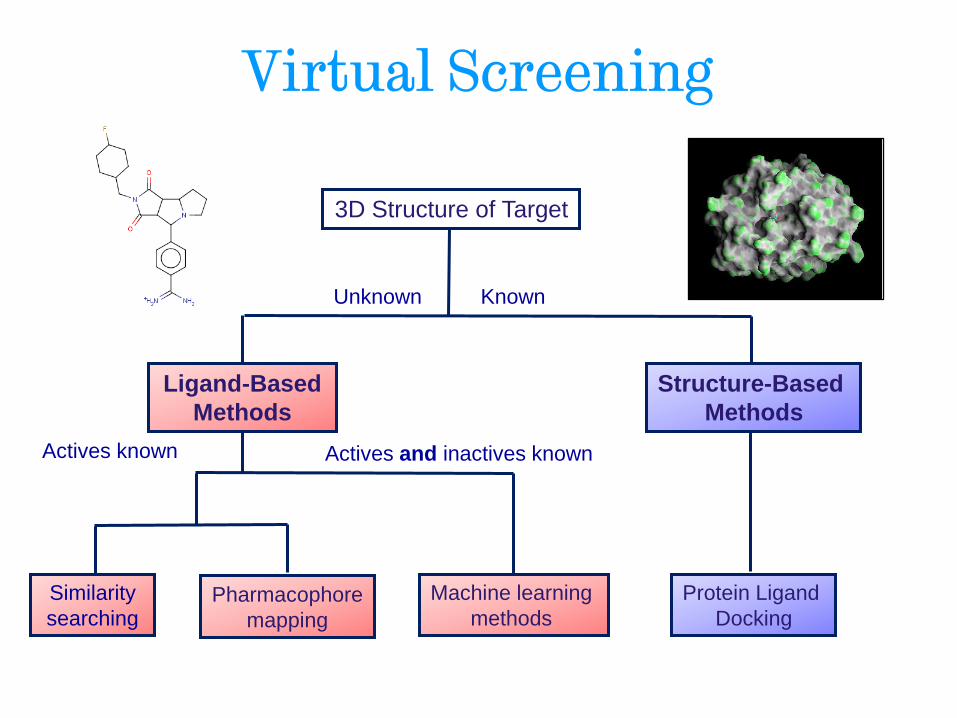
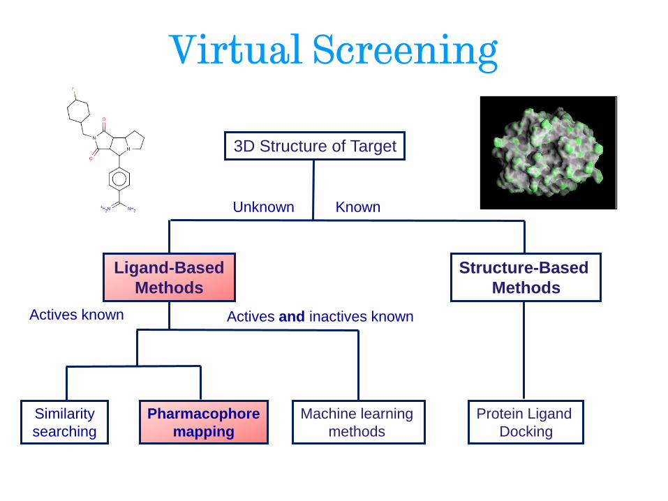
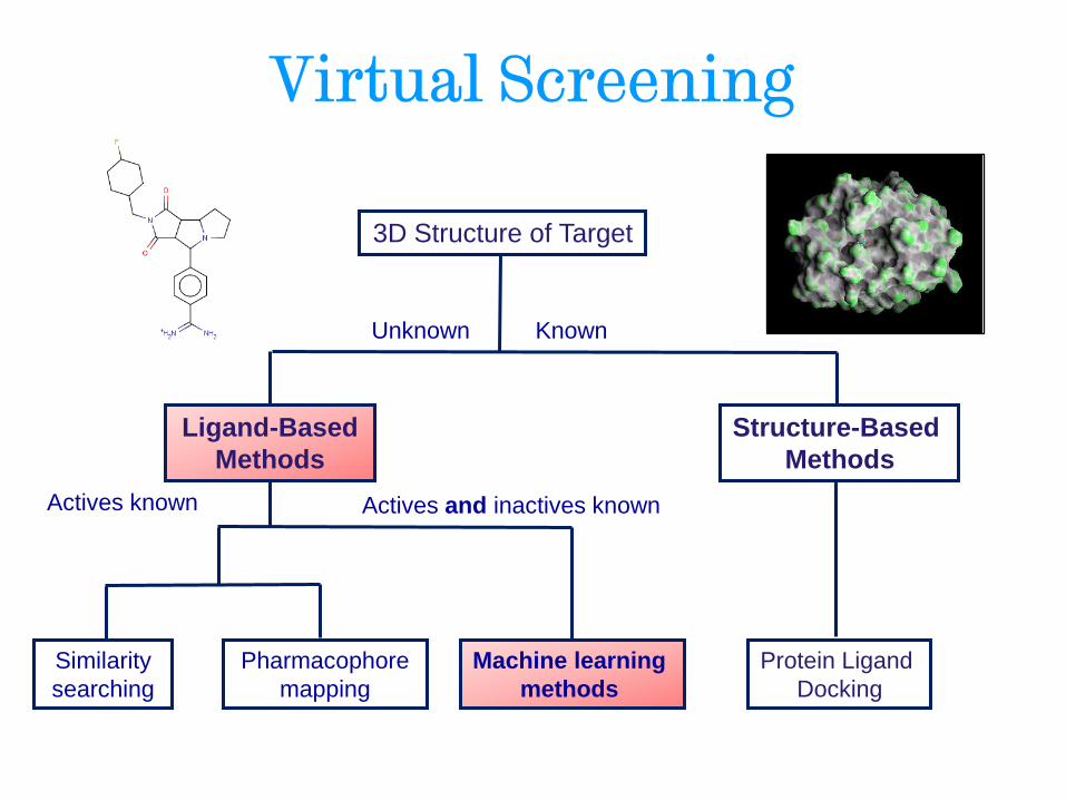
Virtual Screening
Ligand-Based
Methods
Structure-Based
Methods
Unknown
3D Structure of Target
Known
Actives known Actives and inactives known
Machine learning
methods Pharmacophore
mapping
Similarity
searching
Protein Ligand
Docking

Virtual Screening
Ligand-Based
Methods
Structure-Based
Methods
Unknown
3D Structure of Target
Known
Actives known Actives and inactives known
Machine learning
methods Pharmacophore
mapping
Similarity
searching
Protein Ligand
Docking
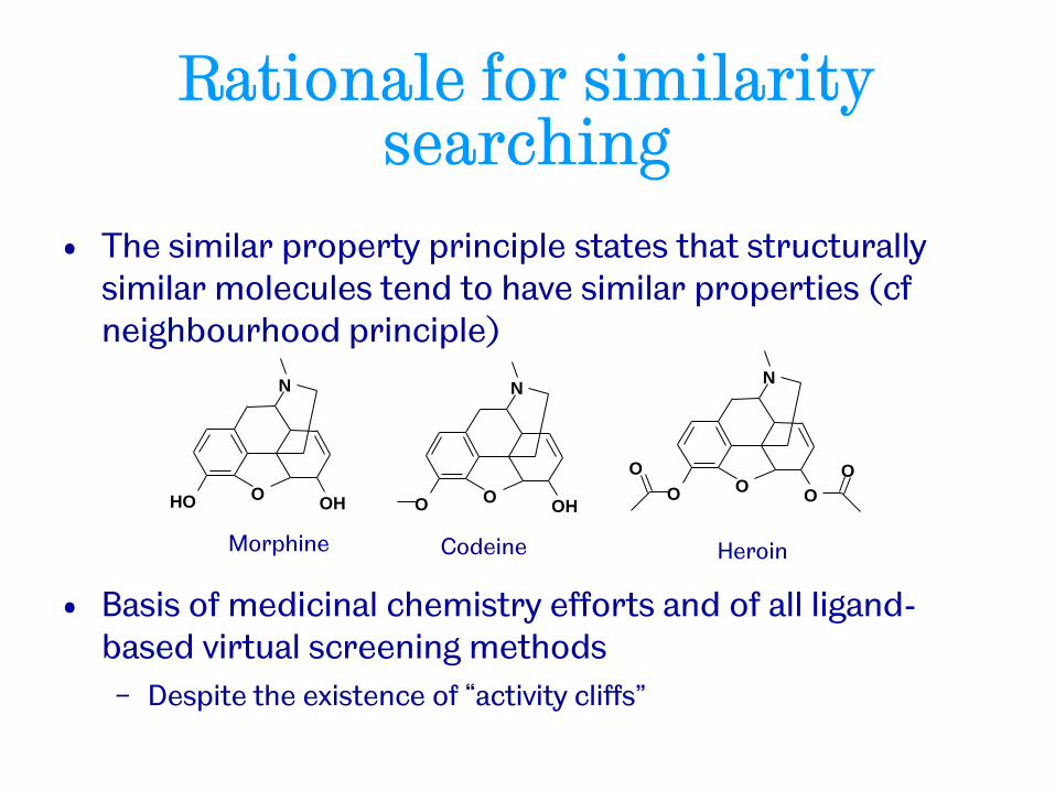
Rationale for similarity searching
• The similar property principle states that structurally similar molecules tend to have similar properties (cf neighbourhood principle)
• Basis of medicinal chemistry efforts and of all ligand-based virtual screening methods
− Despite the existence of “activity cliffs”
N
O O H O H
Morphine
N
O O H O
Codeine
N
O O O
O O
Heroin
Similarity-based virtual screening
• Given an active reference structure rank order a database of compounds on similarity to the reference
• Select the top ranking compounds for biological testing
• Requires a way of measuring the similarity of a pair of compounds
• But similarity is inherently subjective, so need to provide a quantitative basis, a similarity measure, for ranking structures
• There is no single measure of similarity
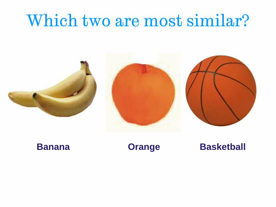
Which two are most similar?
Banana Orange Basketball
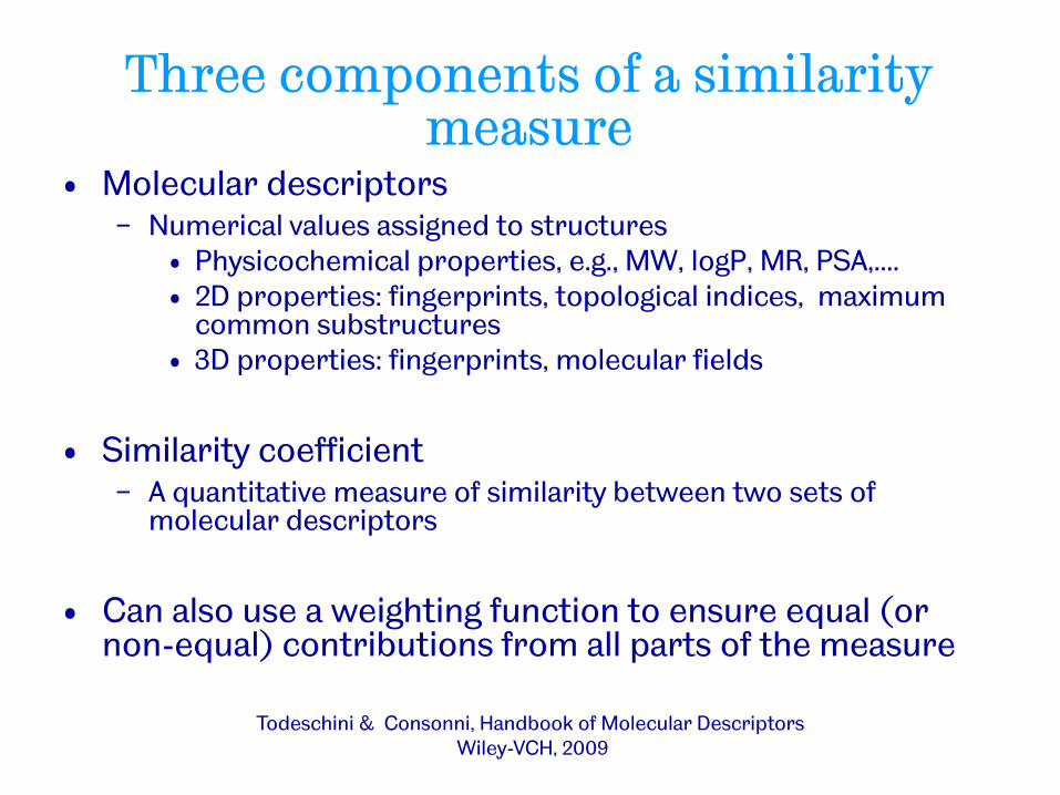
Three components of a similarity measure
• Molecular descriptors − Numerical values assigned to structures
• Physicochemical properties, e.g., MW, logP, MR, PSA,.... • 2D properties: fingerprints, topological indices, maximum
common substructures • 3D properties: fingerprints, molecular fields
• Similarity coefficient − A quantitative measure of similarity between two sets of
molecular descriptors
• Can also use a weighting function to ensure equal (or non-equal) contributions from all parts of the measure
Todeschini & Consonni, Handbook of Molecular Descriptors Wiley-VCH, 2009

2D fingerprints: molecules represented as binary vectors
• Each bit in the bit string (binary vector) represents one molecular fragment. Typical length is ~1000 bits
• The bit string for a molecule records the presence (“1”) or absence (“0”) of each fragment in the molecule
• Originally developed for speeding up substructure search
− for a query substructure to be present in a database molecule each bit set to “1” in the query must also be set to “1” in the database structure
• Similarity is based on determining the number of bits that are common to two structures
C C C
C
C
C C C
O

C
C
N C
C C
C
C N
C
C
C
C C
C
C
C
C
C
C
N C
C
N
C
a. Augmented Atom C rs C rd C rs C
b. Atom Sequence C rs C rs C rd C
c. Bond Sequence AA rs AA rs AA rd AA
d. Ring Composition N rs C rd C rs C rs C rs
e. Ring Fusion XX3 XX3 XX3 XX2 XX2
f. Atom Pair N 0;3 - 2 - C 0;3
Example fragments
Dictionary-based fingerprints: pre-defined fragments each of which maps to a single bit. Examples include MACCS Keys, BCI fps
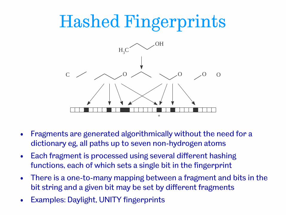
Hashed Fingerprints
• Fragments are generated algorithmically without the need for a dictionary eg, all paths up to seven non-hydrogen atoms
• Each fragment is processed using several different hashing functions, each of which sets a single bit in the fingerprint
• There is a one-to-many mapping between a fragment and bits in the bit string and a given bit may be set by different fragments
• Examples: Daylight, UNITY fingerprints
*
CH3
OH
C OO O O

Other descriptors: Circular substructures
• Each atom is represented by a string of integers obtained by an adaptation of the Morgan algorithm
• Pipeline Pilot (Accelrys) descriptors, e.g., ECFP2, ECFP4, ECFP6, FCFP2,....
• ECFP fragments encode atomic type, charge and mass
• FCFP fragments encode six generalised atom-types
• 2, 4 or 6 denotes the diameter (in bonds) of the circular substructure
• RDKit variant: Morgan, FeatMorgan
N
NN
NH
N
O
OH
O
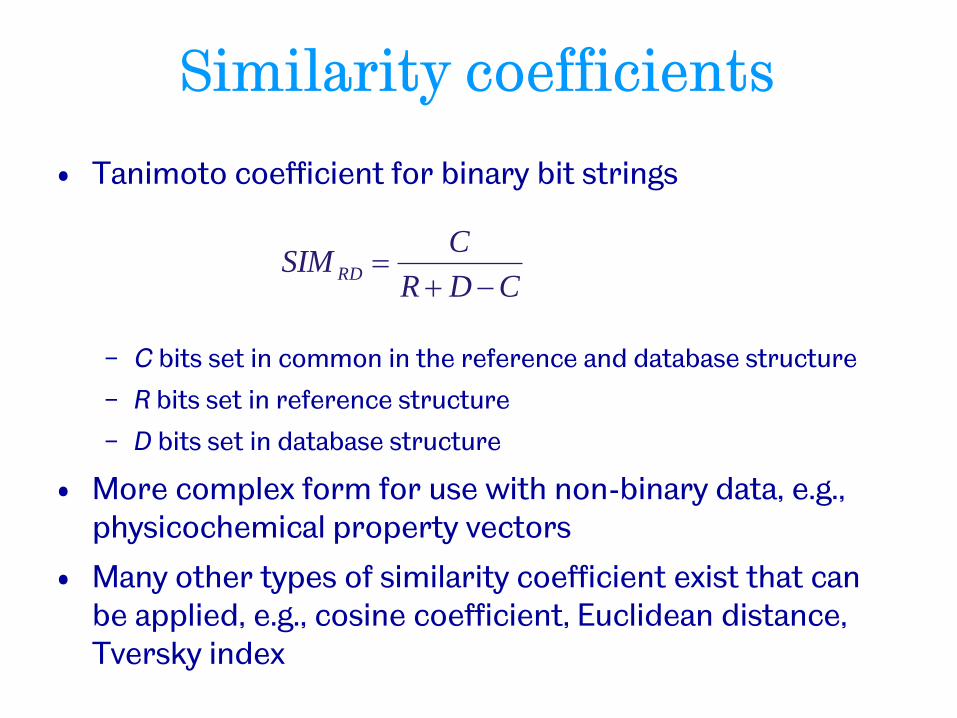
Similarity coefficients
• Tanimoto coefficient for binary bit strings
− C bits set in common in the reference and database structure
− R bits set in reference structure
− D bits set in database structure
• More complex form for use with non-binary data, e.g., physicochemical property vectors
• Many other types of similarity coefficient exist that can be applied, e.g., cosine coefficient, Euclidean distance, Tversky index
CDR
CSIM RD
Limitations of traditional 2D descriptors
N
O O H O H
Morphine
N
O O H O
Codeine 0.99 similar
N
O O O
O O
Heroin 0.95 similar
N
O
Methadone 0.20 similar
Daylight fingerprints;
Tanimoto similarities
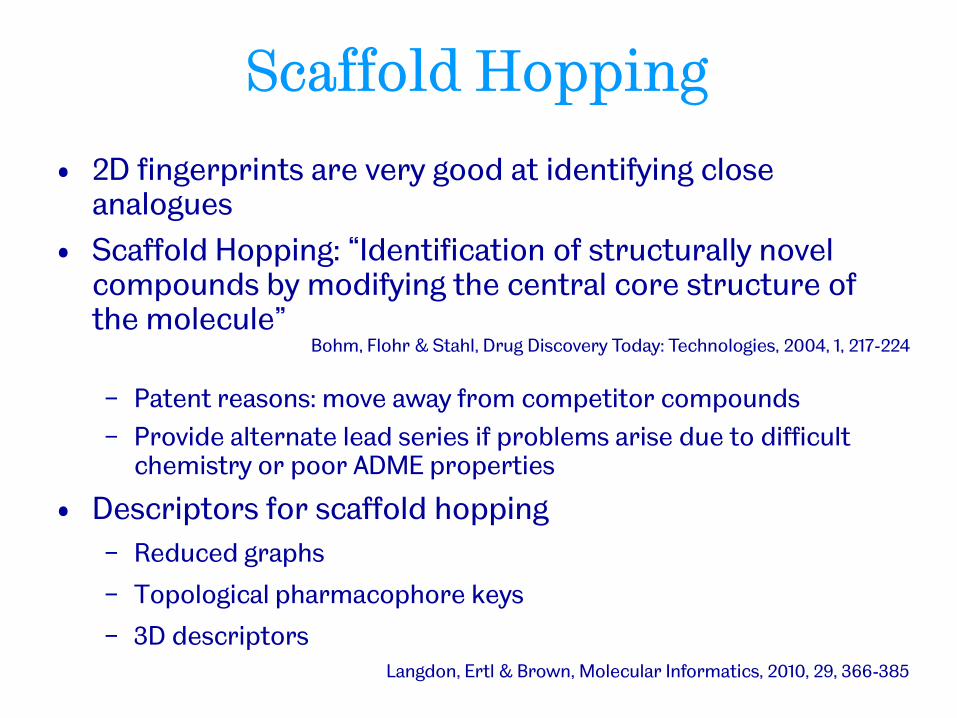
Scaffold Hopping
• 2D fingerprints are very good at identifying close analogues
• Scaffold Hopping: “Identification of structurally novel compounds by modifying the central core structure of the molecule”
− Patent reasons: move away from competitor compounds
− Provide alternate lead series if problems arise due to difficult chemistry or poor ADME properties
• Descriptors for scaffold hopping
− Reduced graphs
− Topological pharmacophore keys
− 3D descriptors
Bohm, Flohr & Stahl, Drug Discovery Today: Technologies, 2004, 1, 217-224
Langdon, Ertl & Brown, Molecular Informatics, 2010, 29, 366-385

Scaffold Hops
Cyclooxygenase inhibitors
Bohm, Flohr & Stahl, Scaffold hopping. Drug Discovery Today: Technologies, 2004, 1, 217-224
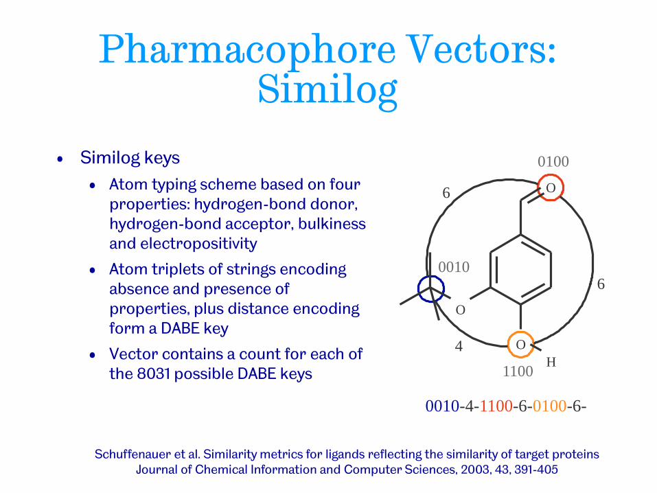
Pharmacophore Vectors: Similog
• Similog keys
• Atom typing scheme based on four properties: hydrogen-bond donor, hydrogen-bond acceptor, bulkiness and electropositivity
• Atom triplets of strings encoding absence and presence of properties, plus distance encoding form a DABE key
• Vector contains a count for each of the 8031 possible DABE keys
0010-4-1100-6-0100-6-
0100
0010
1100
6
6
4
O
O
H
O
Schuffenauer et al. Similarity metrics for ligands reflecting the similarity of target proteins Journal of Chemical Information and Computer Sciences, 2003, 43, 391-405
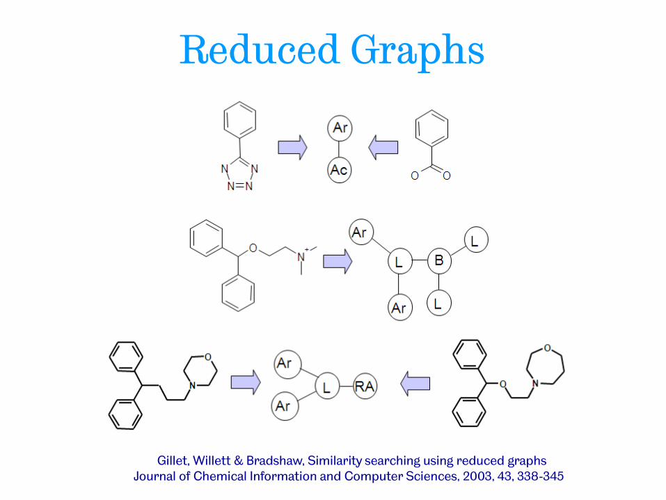
Reduced Graphs
Gillet, Willett & Bradshaw, Similarity searching using reduced graphs Journal of Chemical Information and Computer Sciences, 2003, 43, 338-345
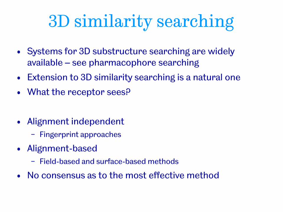
3D similarity searching
• Systems for 3D substructure searching are widely available – see pharmacophore searching
• Extension to 3D similarity searching is a natural one
• What the receptor sees?
• Alignment independent
− Fingerprint approaches
• Alignment-based
− Field-based and surface-based methods
• No consensus as to the most effective method
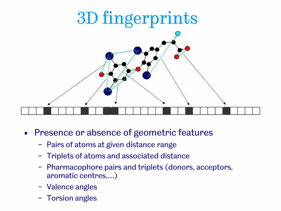
3D fingerprints
• Presence or absence of geometric features − Pairs of atoms at given distance range
− Triplets of atoms and associated distance
− Pharmacophore pairs and triplets (donors, acceptors, aromatic centres,....)
− Valence angles
− Torsion angles

Alignment-based 3D similarity
• Shape-based − ROCS (Rapid Overlay of Chemical Structures)
− Molecules are aligned in 3D
− Similarity score is based on common volume
Nicholls et al, Molecular Shape and Medicinal Chemistry; A Perspective. Journal of Medicinal Chemistry, 2010, 53, 3862-3886
Copyright © 2010 American Chemical Society
CBA
CAB
VVV
VSIM
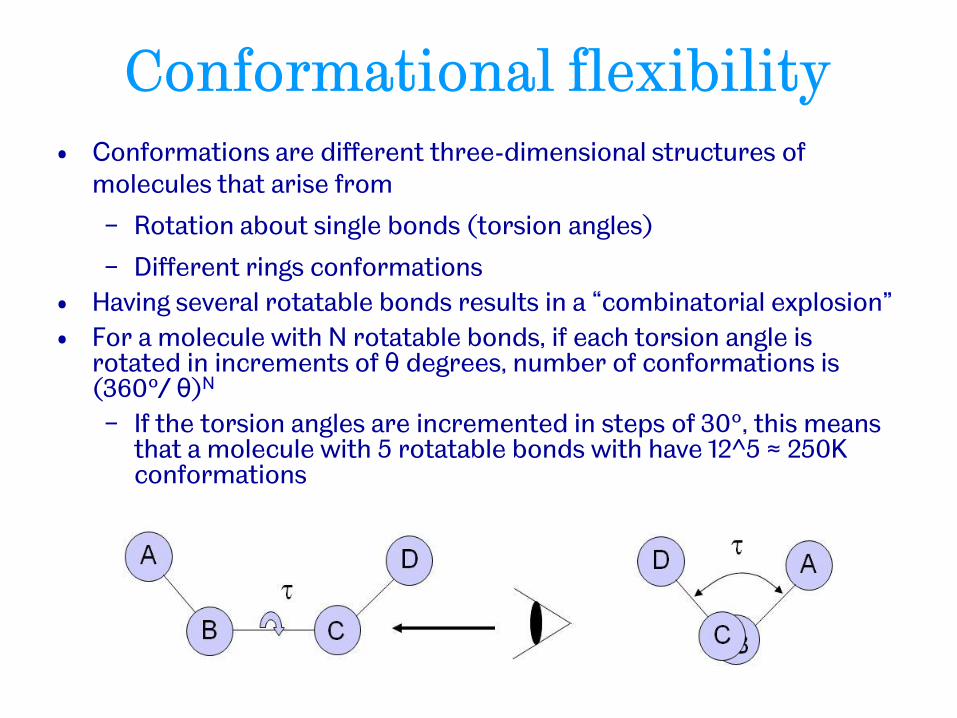
Conformational flexibility • Conformations are different three-dimensional structures of
molecules that arise from
− Rotation about single bonds (torsion angles)
− Different rings conformations
• Having several rotatable bonds results in a “combinatorial explosion”
• For a molecule with N rotatable bonds, if each torsion angle is rotated in increments of θ degrees, number of conformations is (360º/ θ)N
− If the torsion angles are incremented in steps of 30º, this means that a molecule with 5 rotatable bonds with have 12^5 ≈ 250K conformations
Two approaches to handling conformational flexibility
Conformer selection
• When a new molecule is to be registered in a database, a conformational analysis is used to select diverse conformers spanning the low-energy conformational space
• Each such conformer is loaded into the database and then searched as if it was a single, rigid structure
• Trade-off between effectiveness of coverage (selection of many conformers) and efficiency of searching (selection of few conformers)
Exploration of conformational space • Use of triangle smoothing to
identify min-max distances between each atom-pair
• Creation of a distance-range (rather than a distance) graph for each database structure
• Screen and graph search of the min-max distance data using appropriately modified algorithms
• Final conformational analysis (by varying torsional angles) of the hits resulting from the screen/graph searches

3D similarity
• Computationally more expensive than 2D methods
• Requires consideration of conformational flexibility − Rigid search - based on a single conformer
− Flexible search • Conformation explored at search time
• Ensemble of conformers generated prior to search time with each conformer of each molecule considered in turn
• How many conformers are required?
• Methods that require aligning molecules are more costly than vector-based calculations
Evaluation of similarity methods
• Retrospective search
• For a reference compound of known activity, search against a database that contains other actives and decoy compounds
− Determine where the active compounds appear in the ranked list
− A good similarity measure will cluster the known actives at the top of the ranking
− Performance measures: enrichment factors, AUC, BEDROC, .....
• Comparative studies suggest that 2D fingerprints are most effective
− Good at identifying "me-too" compounds but less good at scaffold hopping
• R.P. Sheridan and S.K. Kearsley (2002) Drug Discovery Today, 7, 903-911
− “We have come to regard looking for ‘the best’ way of searching chemical databases as a futile exercise. In both retrospective and prospective studies, different methods select different subsets of actives for the same biological activity and the same method might work better on some activities than others”
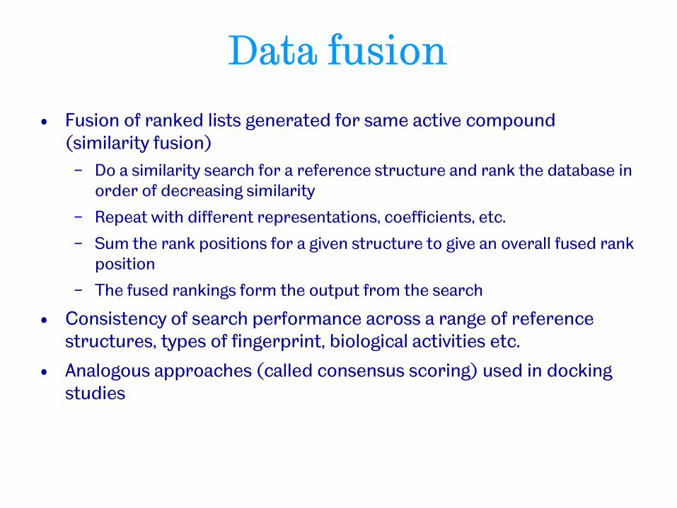
Data fusion
• Fusion of ranked lists generated for same active compound (similarity fusion)
− Do a similarity search for a reference structure and rank the database in order of decreasing similarity
− Repeat with different representations, coefficients, etc.
− Sum the rank positions for a given structure to give an overall fused rank position
− The fused rankings form the output from the search
• Consistency of search performance across a range of reference structures, types of fingerprint, biological activities etc.
• Analogous approaches (called consensus scoring) used in docking studies
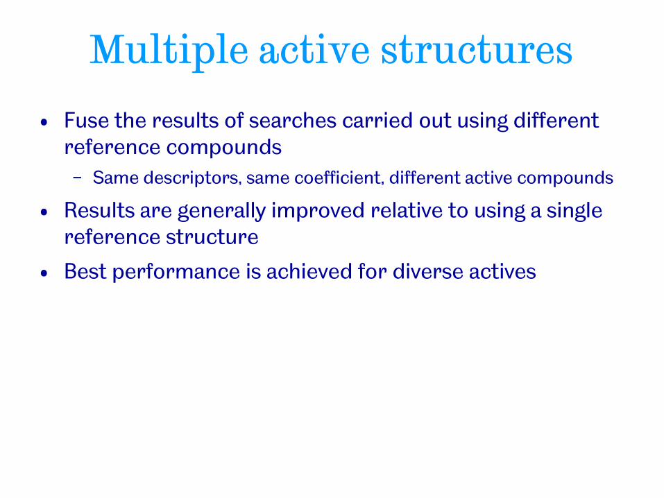
Multiple active structures
• Fuse the results of searches carried out using different reference compounds
− Same descriptors, same coefficient, different active compounds
• Results are generally improved relative to using a single reference structure
• Best performance is achieved for diverse actives
Virtual Screening
Ligand-Based
Methods
Structure-Based
Methods
Unknown
3D Structure of Target
Known
Actives known Actives and inactives known
Machine learning
methods
Pharmacophore
mapping
Similarity
searching
Protein Ligand
Docking
Multiple actives known: phamacophore searching
(with thanks to Stefan Senger, GSK)

• A pharmacophore is the ensemble of steric and electronic features that is necessary to ensure the optimal supramolecular interactions with a specific biological target structure and to trigger (or to block) its biological response
Pharmacophore Definition
Glossary of terms used in Medicinal Chemistry (IUPAC Recommendations 1998) Pure & Appl. Chem. 1998, 70(5), 1129-1143 http://dx.doi.org/10.1351/pac199870051129).
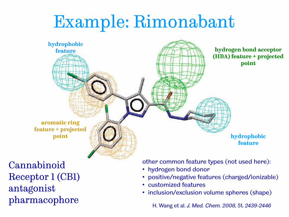
H. Wang et al. J. Med. Chem. 2008, 51, 2439-2446
hydrogen bond acceptor (HBA) feature + projected
point
hydrophobic feature
hydrophobic feature
aromatic ring feature + projected
point
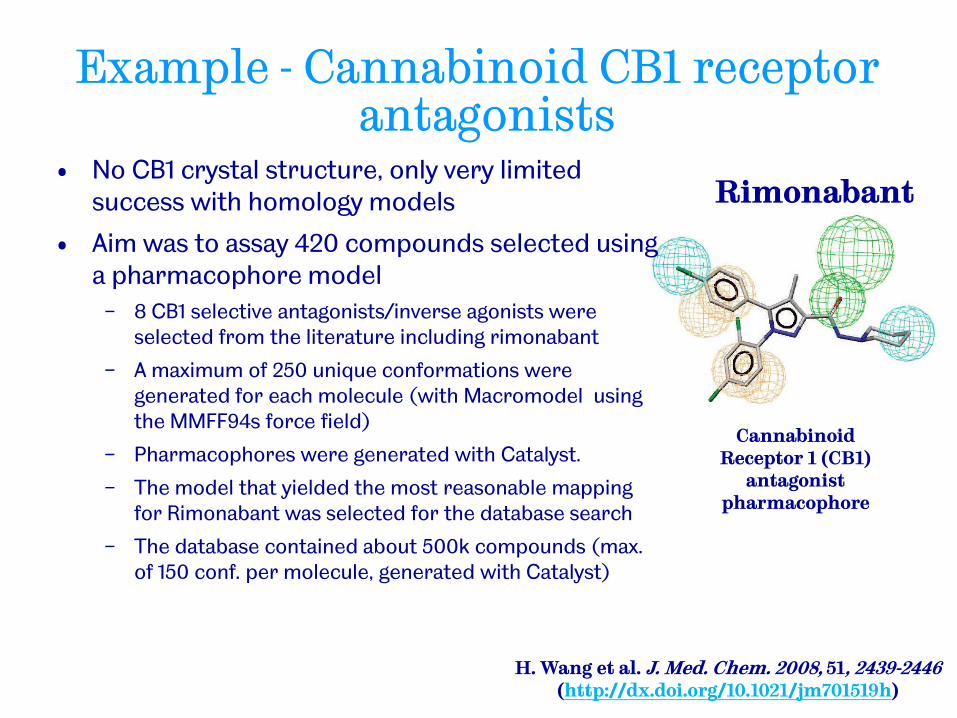
Cannabinoid Receptor 1 (CB1) antagonist pharmacophore
other common feature types (not used here): • hydrogen bond donor • positive/negative features (charged/ionizable) • customized features • inclusion/exclusion volume spheres (shape)
Example: Rimonabant
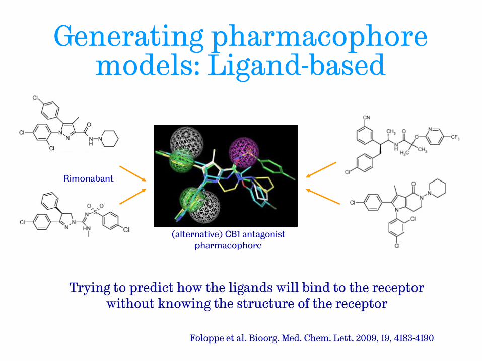
Generating pharmacophore models: Ligand-based
Foloppe et al. Bioorg. Med. Chem. Lett. 2009, 19, 4183-4190
Rimonabant
(alternative) CB1 antagonist pharmacophore
Trying to predict how the ligands will bind to the receptor without knowing the structure of the receptor
Pharmacophore generation methods
• Pharmacophoric features in each ligand identified
− Donors, acceptors, hydrophobic groups,...
− Often SMARTs-based to allow user-definitions
• Ligands aligned such that corresponding features are overlaid
• Conformational space explored
− On-the-fly eg using a genetic algorithm
− Generating ensemble of conformations with each conformer considered in turn
• Given the undetermined nature of the problem it is unlikely that a single correct solution will be found
• Pharmacophore hypotheses are scored
− eg number of features, goodness of fit to features, conformational energy, volume of the overlay, rarity of the pharmacophore,....
Ligand-based pharmacophores: practical aspects
• Select a ‘representative’ set of actives
− Most methods assume similar binding modes
− One or more rigid molecules are preferred
− The ligands should be diverse (otherwise too many common features that are not involved in binding)
• Prepare molecules (e.g. tautomeric form, protonation state), generate 3D structure and conformations (if required)
• Use pharmacophore software/tool to generate pharmacophores (biased or unbiased?)
• Select preferred pharmacophore model(s) and validate them
− Visual inspection
− Do the “actives” fit the pharmacophore?
− Can the pharmacophore separate actives from decoys?

D. Schulster et al. Bioorg. Med. Chem. 2011, 19, 7168-7180 (http://dx.doi.org/10.1016/j.bmc.2011.09.056)
U. Grienke et al. Bioorg. Med. Chem. 2011, 19, 6779-6791 (http://dx.doi.org/10.1016/j.bmc.2011.09.039)
Pharmacophore contains five hydrophobic features, one hydrogen bond acceptor feature, and 27 exclusion spheres
PDB entry 1osh, farnesoid X receptor (FXR, a ligand-dependent transcription factor)
Structure-based pharmacophores
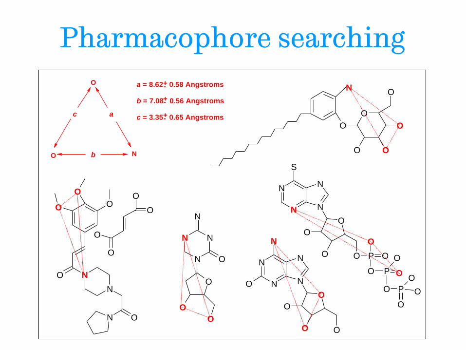
Pharmacophore searching
O
O N
a
b
c
a = 8.62 0.58 Angstroms
b = 7.08 0.56 Angstroms
c = 3.35 0.65 Angstroms +-
+-
+-
O
O
O
O
OO
N
O
O
O
N
N
N O
O
O
O
O
O
N
N
N
N
S
O
O
O O P O
O
O P O
O P
O
O
O
ON
N
N
N
N
O
O
O O
O
N
N
N
O
N
O
O
O
Database searching • Conformational search
− On-the-fly
− Ensemble of conformers
• Database search should be “compatible” with parameters used to generate the pharmacophore
− The same pharmacophore feature definitions should be used to describe the database structures as were used to generate the pharmacophore
− The database should be generated using the same protocol as used to generate the pharmacophore
− What tolerance should be used to allow a match?
• If two pharmacophore features are separated by 5Å what distance range is acceptable: 4.5-5.5Å; 4-6Å?
• Should all tolerances be the same?
• What effect does this have on recall and precision?
− Can exclusion/inclusion volumes be used?

Select actives
Generate conformers
Generate (Modify)
pharmacophore models
Validation 1: Map actives back on
pharmacophore
Validation 2: Search validation
database – enrichment, specificity, sensitivity?
Prioritise/select pharmacophore
model(s)
Perform search/mapping(s)
Generate/select ‘compatible’ compound database
Select actives + inactives/decoys
for validation
Generate ‘compatible’ validation database
Filter (availability, properties,
novelty, visually inspect
mappings,…)
Select compounds
for screening
Virtual screening
Pharmacophore-based VS: workflow
H. Wang et al. J. Med. Chem. 2008, 51, 2439-2446 (http://dx.doi.org/10.1021/jm701519h)
Rimonabant
Cannabinoid Receptor 1 (CB1)
antagonist pharmacophore
Example - Cannabinoid CB1 receptor antagonists
• No CB1 crystal structure, only very limited success with homology models
• Aim was to assay 420 compounds selected using a pharmacophore model
− 8 CB1 selective antagonists/inverse agonists were selected from the literature including rimonabant
− A maximum of 250 unique conformations were generated for each molecule (with Macromodel using the MMFF94s force field)
− Pharmacophores were generated with Catalyst.
− The model that yielded the most reasonable mapping for Rimonabant was selected for the database search
− The database contained about 500k compounds (max. of 150 conf. per molecule, generated with Catalyst)
• The pharmacophore search resulted in 22794 hits (approx. 5% of the database)
• Stepwise filtering 300 < MW < 550 (18693 compounds remaining) availability as solid > 2 mg (10581 compounds remaining) modified Lipinski’s rule of five (7247 compounds remaining)
• A Bayesian model built from compounds in the MDDR database was used to rank the remaining compounds (using the FCFP6 fingerprints in Pipeline Pilot)
• The top ranking 2100 were selected
• Clustering using the maximum dissimilarity clustering algorithm. 420 clusters were generated and from each cluster the compound with the highest Bayesian score was selected.
H. Wang et al. J. Med. Chem. 2008, 51, 2439-2446
(http://dx.doi.org/10.1021/jm701519h)
Example (continued)

• 420 compounds were screened at a single concentration. Five compounds showed more than 50% inhibition. All five compounds confirmed in the full curve assay.
− Approx. 1% screening hit rate
• One compound has a Ki of less than 100 nM.
Rimonabant
Cannabinoid Receptor 1 (CB1) antagonist pharmacophore
H. Wang et al. J. Med. Chem. 2008, 51, 2439-2446 (http://dx.doi.org/10.1021/jm701519h)
Example (continued)

Software Source Recent published use cases
Catalyst (Discovery Studio)
Accelrys http://dx.doi.org/10.1007/s00894-011-1105-5 http://dx.doi.org/10.1016/j.bmcl.2010.12.131
GASP Tripos http://dx.doi.org/10.1016/j.jmgm.2010.02.004
GALAHAD Tripos http://dx.doi.org/10.1016/j.bmc.2011.09.016 http://dx.doi.org/10.1016/j.ejmech.2010.09.012
Ligandscout Inte:ligand http://dx.doi.org/10.1016/j.eplepsyres.2011.08.016
MOE Chemical Computing Group
http://dx.doi.org/10.1007/s10822-011-9442-0 http://dx.doi.org/10.1016/j.ejmech.2010.07.020
Phase Schrödinger http://10.1111/j.1747-0285.2011.01130.x http://cs-test.ias.ac.in/cs/Volumes/100/12/1847.pdf
Examples (by no means comprehensive):
(Commercial) software

Some references for pharmacophores
• A. R. Leach, V. J. Gillet, R. A. Lewis, R. Taylor Three-Dimensional Pharmacophore Methods in Drug Discovery J. Med. Chem. 2010, 53, 539-558 (http://dx.doi.org/10.1021/jm900817u)
• T. Seidel, G. Ibis, F. Bendix, G. Wolber Strategies for 3D pharmacophore-based virtual screening Drug Disc. Today: Technologies 2010, 7, e221-e228 (http://dx.doi.org/10.1016/j.ddtec.2010.11.004)
• G. Hessler, K.-H. Baringhaus The scaffold hopping potential of pharmacophores Drug Disc. Today: Technologies 2010, 7, e263-e269 (http://dx.doi.org/10.1016/j.ddtec.2010.09.001)
• M. Hein, D. Zilian, C. A. Sotriffer Docking compared to 3D-pharmacophores: the scoring function challenge Drug Disc. Today: Technologies 2010, 7, e2229-e236 (http://dx.doi.org/10.1016/j.ddtec.2010.12.003)
• F. Caporuscio, A. Tafi Pharmacophore Modelling: A Forty Year Old Approach and its Modern Synergies Curr. Med. Chem. 2011, 18, 2543-2553
• I. Wallach Pharmacophore Interference and its Application to Computational Drug Discovery Drug Dev. Res. 2011, 72, 17-25 (http://dx.doi.org/10.1002/ddr.20398)
Virtual Screening
Ligand-Based
Methods
Structure-Based
Methods
Unknown
3D Structure of Target
Known
Actives known Actives and inactives known
Machine learning
methods
Pharmacophore
mapping
Similarity
searching
Protein Ligand
Docking

Structure-Activity Relationship Modelling
• Use knowledge of known active and known inactive compounds to build a predictive model
• Quantitative-Structure Activity Relationships (QSARs)
− Long established (Hansch analysis, Free-Wilson analysis)
− Generally restricted to small, homogeneous datasets eg lead optimisation
• Structure-Activity Relationships (SARs)
− “Activity” data is usually treated qualitatively
− Can be used with data consisting of diverse structural classes and multiple binding modes
− Some resistance to noisy data (HTS data)
− Resulting models used to prioritise compounds for lead finding (not to identify candidates or drugs)

C3 C1 C4 C2 C5
.
.
.
.
.
.
.
.
.
.
.
Lik
elih
oo
d o
f be
ing
ac
tive
Top Ranked Compounds Picked
for Testing Training Set
Known active compounds Known inactive compounds
Model of Activity
Analyse actives
inactives
Untested compounds C1, C2, C3, C4, C5 …
Compute scores
Generalised machine learning method
•Substructural analysis •Recursive partitioning •Support vector machines •K nearest neighbours •Neural networks
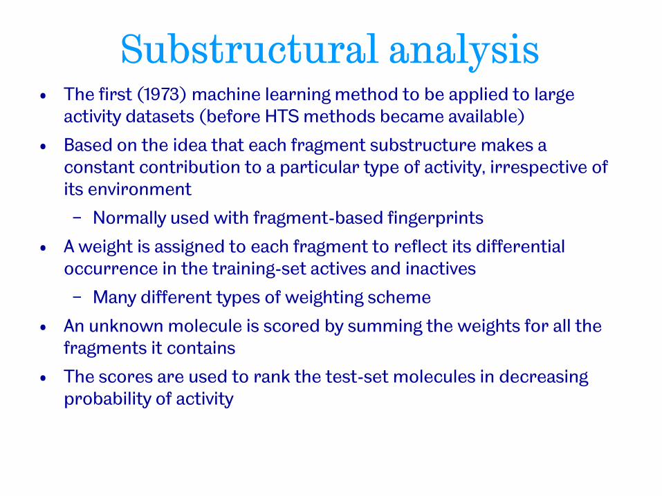
Substructural analysis • The first (1973) machine learning method to be applied to large
activity datasets (before HTS methods became available)
• Based on the idea that each fragment substructure makes a constant contribution to a particular type of activity, irrespective of its environment
− Normally used with fragment-based fingerprints
• A weight is assigned to each fragment to reflect its differential occurrence in the training-set actives and inactives
− Many different types of weighting scheme
• An unknown molecule is scored by summing the weights for all the fragments it contains
• The scores are used to rank the test-set molecules in decreasing probability of activity
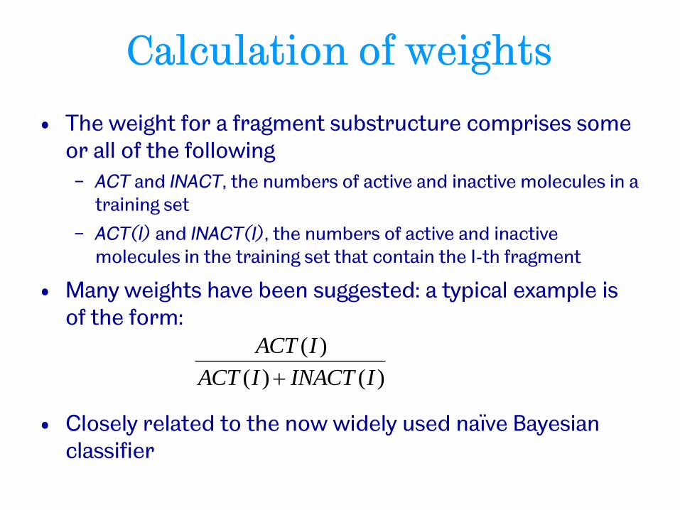
Calculation of weights
• The weight for a fragment substructure comprises some or all of the following
− ACT and INACT, the numbers of active and inactive molecules in a training set
− ACT(I) and INACT(I), the numbers of active and inactive molecules in the training set that contain the I-th fragment
• Many weights have been suggested: a typical example is of the form:
• Closely related to the now widely used naïve Bayesian classifier
)()(
)(
IINACTIACT
IACT

Recursive Partitioning • Classification approach that constructs a decision tree
from qualitative data
− active/inactive, soluble/insoluble, toxic/non-toxic
• Identification of a rule that gives the best statistical split into classes, with the lowest rate of misclassification
− Example drug|non-drug: MW < 500|MW > 500
• Repeat on each set coming from the previous split until no more reasonable splits can be found
• Can generate good models but with poor predictive power if used without care
− Use leave-many-out strategies to validate
− Easy to interpret/drive what-next decisions
Hamman F, Gutmann H. Voigt N, Helma C, Drewe J. Prediction of adverse drug reactions using decision tree modeling. Clin Pharmacol Ther, 2010, 88, 52-59.

Example
Test compounds are dropped through the tree. Prediction depends on whether they fall into “active” or inactive nodes”

Virtual Screening
Ligand-Based
Methods
Structure-Based
Methods
Unknown
3D Structure of Target
Known
Actives known Actives and inactives known
Machine learning
methods
Pharmacophore
mapping
Similarity
searching
Protein Ligand
Docking
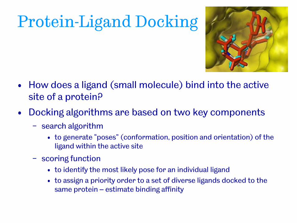
Protein-Ligand Docking
• How does a ligand (small molecule) bind into the active site of a protein?
• Docking algorithms are based on two key components
− search algorithm
• to generate “poses” (conformation, position and orientation) of the ligand within the active site
− scoring function
• to identify the most likely pose for an individual ligand
• to assign a priority order to a set of diverse ligands docked to the same protein – estimate binding affinity
The search space • The difficulty with protein–ligand docking is in part
due to the fact that it involves many degrees of freedom
− The translation and rotation of one molecule relative to another involves six degrees of freedom
− These are in addition the conformational degrees of freedom of both the ligand and the protein
− The solvent may also play a significant role in determining the protein–ligand geometry (often ignored though)
• The search algorithm generates poses, orientations of particular conformations of the molecule in the binding site − Tries to cover the search space, if not exhaustively, then as
extensively as possible
− There is a tradeoff between time and search space coverage
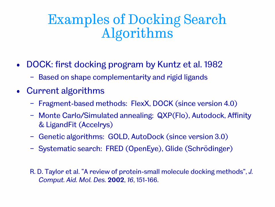
Examples of Docking Search Algorithms
• DOCK: first docking program by Kuntz et al. 1982
− Based on shape complementarity and rigid ligands
• Current algorithms
− Fragment-based methods: FlexX, DOCK (since version 4.0)
− Monte Carlo/Simulated annealing: QXP(Flo), Autodock, Affinity & LigandFit (Accelrys)
− Genetic algorithms: GOLD, AutoDock (since version 3.0)
− Systematic search: FRED (OpenEye), Glide (Schrödinger)
R. D. Taylor et al. “A review of protein-small molecule docking methods”, J. Comput. Aid. Mol. Des. 2002, 16, 151-166.
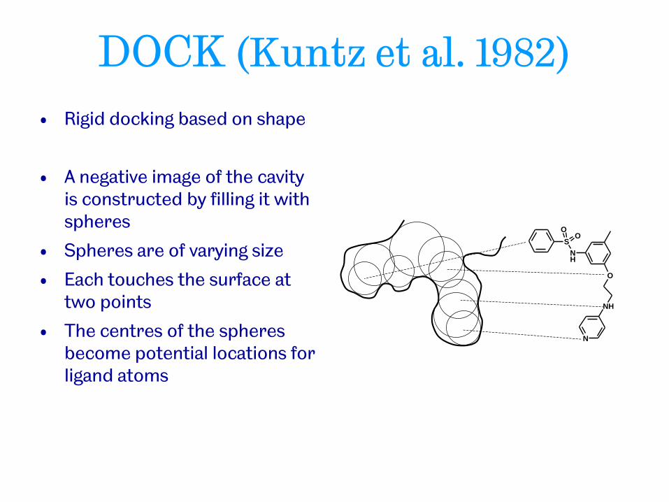
DOCK (Kuntz et al. 1982)
• Rigid docking based on shape
• A negative image of the cavity is constructed by filling it with spheres
• Spheres are of varying size
• Each touches the surface at two points
• The centres of the spheres become potential locations for ligand atoms
SNH
O
NH
O O
N
S
NH
O
NH
OO
N
DOCK
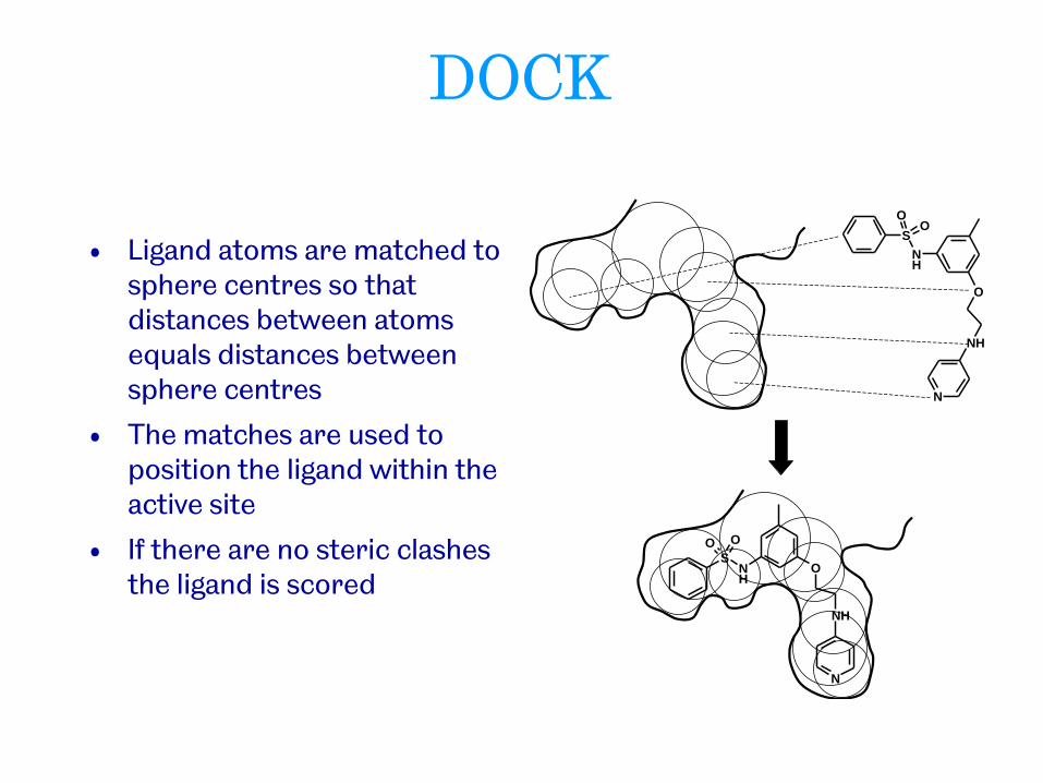
• Ligand atoms are matched to sphere centres so that distances between atoms equals distances between sphere centres
• The matches are used to position the ligand within the active site
• If there are no steric clashes the ligand is scored
SNH
O
NH
O O
N
S
NH
O
NH
OO
N

DOCK
• Many different mappings (poses) are possible
• Each pose is scored based on goodness of fit
• Highest scoring pose is presented to the user
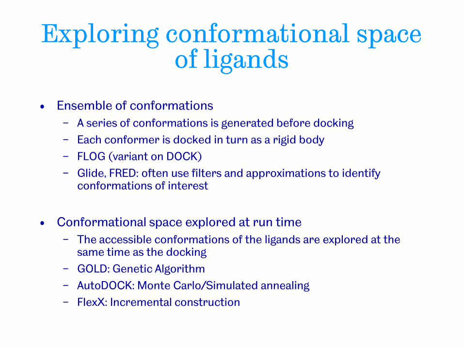
Exploring conformational space of ligands
• Ensemble of conformations
− A series of conformations is generated before docking
− Each conformer is docked in turn as a rigid body
− FLOG (variant on DOCK)
− Glide, FRED: often use filters and approximations to identify conformations of interest
• Conformational space explored at run time
− The accessible conformations of the ligands are explored at the same time as the docking
− GOLD: Genetic Algorithm
− AutoDOCK: Monte Carlo/Simulated annealing
− FlexX: Incremental construction
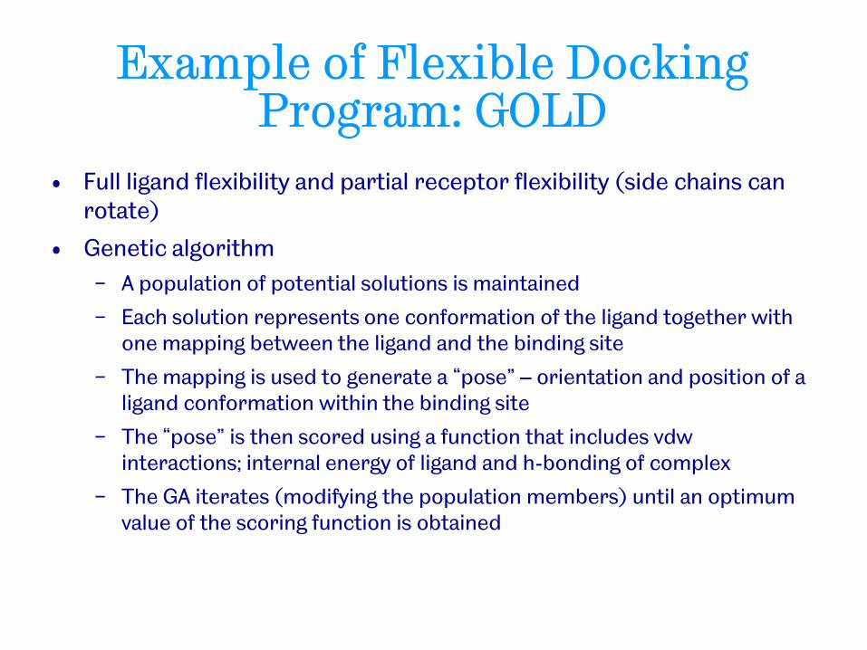
Example of Flexible Docking Program: GOLD
• Full ligand flexibility and partial receptor flexibility (side chains can rotate)
• Genetic algorithm
− A population of potential solutions is maintained
− Each solution represents one conformation of the ligand together with one mapping between the ligand and the binding site
− The mapping is used to generate a “pose” – orientation and position of a ligand conformation within the binding site
− The “pose” is then scored using a function that includes vdw interactions; internal energy of ligand and h-bonding of complex
− The GA iterates (modifying the population members) until an optimum value of the scoring function is obtained
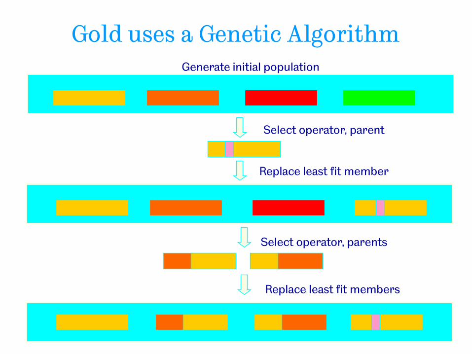
Gold uses a Genetic Algorithm Generate initial population
Select operator, parent
Replace least fit member
Select operator, parents
Replace least fit members
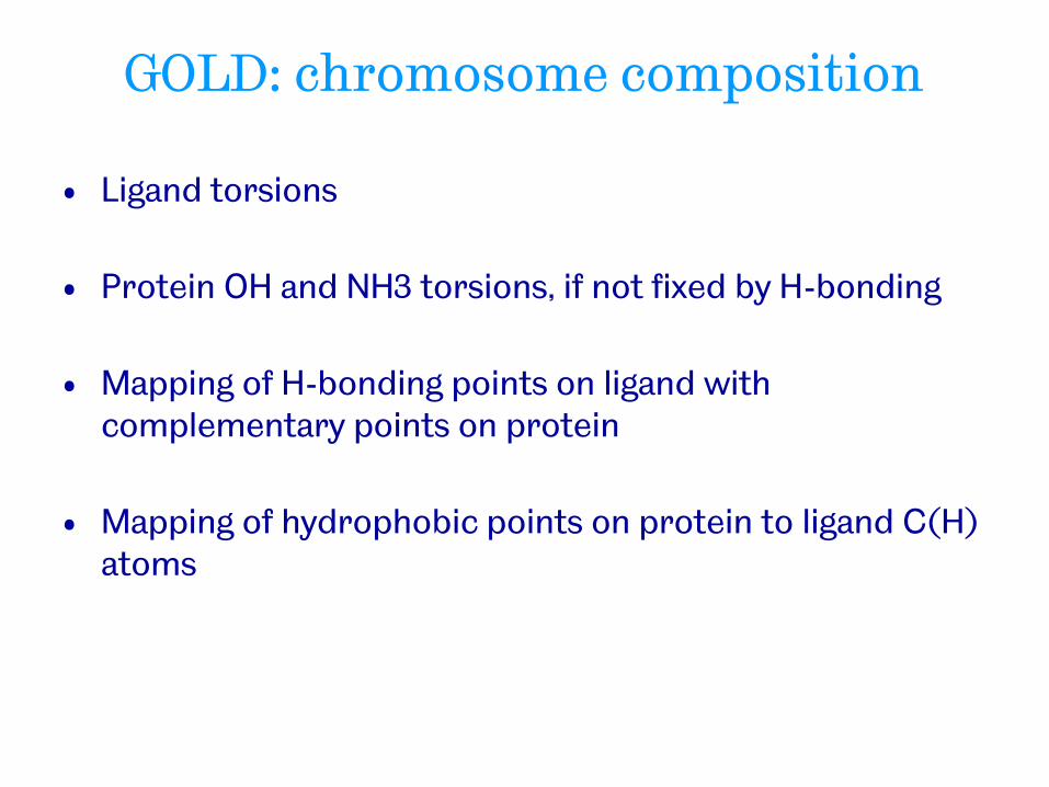
GOLD: chromosome composition
• Ligand torsions
• Protein OH and NH3 torsions, if not fixed by H-bonding
• Mapping of H-bonding points on ligand with complementary points on protein
• Mapping of hydrophobic points on protein to ligand C(H) atoms
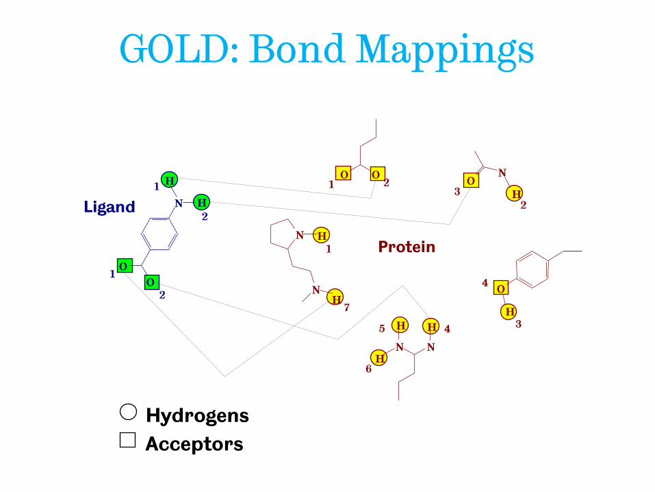
GOLD: Bond Mappings
O
N
N
N N
N O
Ligand
Protein
Hydrogens
Acceptors
N
O
O
O O H
H
H
H
H
H H
H
H
1
1
1
1
2
2
2
2
3
3 4
4
5
6
7
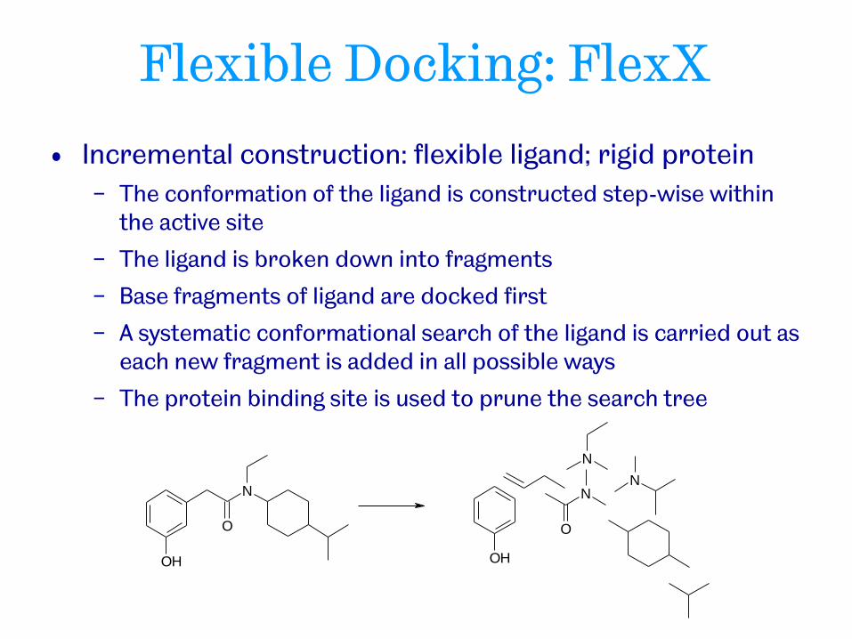
Flexible Docking: FlexX
• Incremental construction: flexible ligand; rigid protein
− The conformation of the ligand is constructed step-wise within the active site
− The ligand is broken down into fragments
− Base fragments of ligand are docked first
− A systematic conformational search of the ligand is carried out as each new fragment is added in all possible ways
− The protein binding site is used to prune the search tree
N
O
OH OH
O
N
N
N
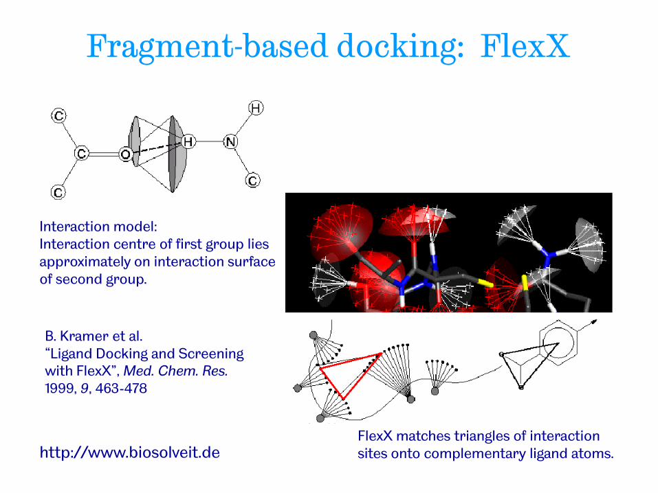
Fragment-based docking: FlexX
FlexX matches triangles of interaction sites onto complementary ligand atoms.
Interaction model: Interaction centre of first group lies approximately on interaction surface of second group.
http://www.biosolveit.de
B. Kramer et al. “Ligand Docking and Screening with FlexX”, Med. Chem. Res. 1999, 9, 463-478
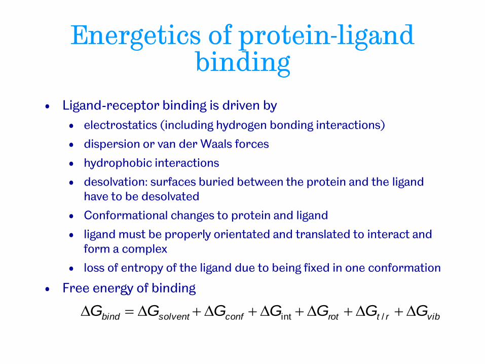
Energetics of protein-ligand binding
vibrtrotconfsolventbind GGGGGGG /int
• Ligand-receptor binding is driven by
• electrostatics (including hydrogen bonding interactions)
• dispersion or van der Waals forces
• hydrophobic interactions
• desolvation: surfaces buried between the protein and the ligand have to be desolvated
• Conformational changes to protein and ligand
• ligand must be properly orientated and translated to interact and form a complex
• loss of entropy of the ligand due to being fixed in one conformation
• Free energy of binding
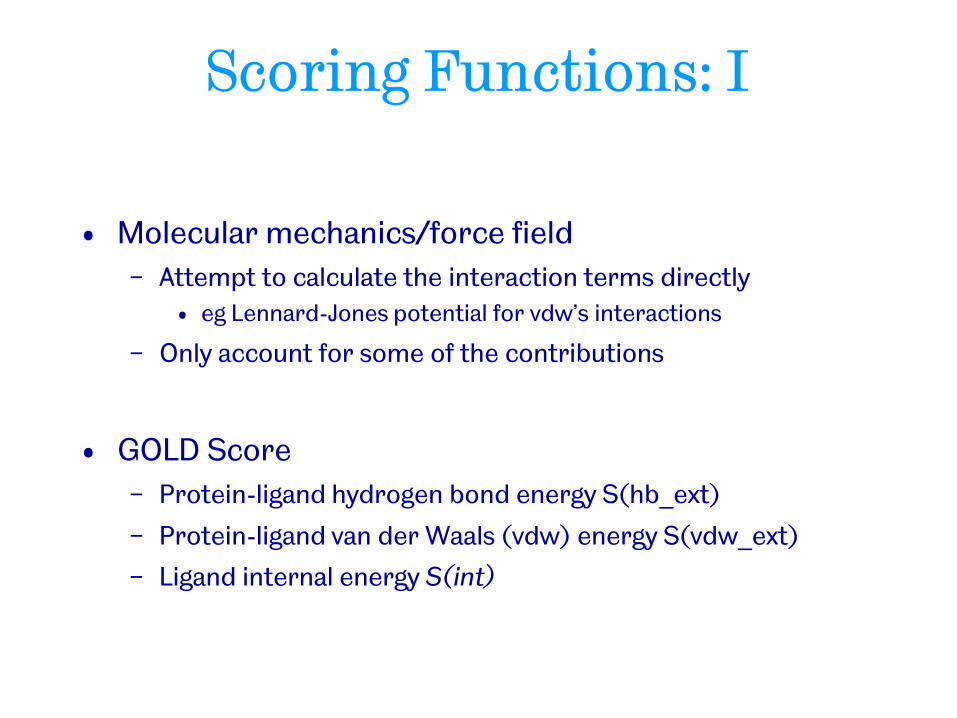
Scoring Functions: I
• Molecular mechanics/force field
− Attempt to calculate the interaction terms directly
• eg Lennard-Jones potential for vdw’s interactions
− Only account for some of the contributions
• GOLD Score
− Protein-ligand hydrogen bond energy S(hb_ext)
− Protein-ligand van der Waals (vdw) energy S(vdw_ext)
− Ligand internal energy S(int)
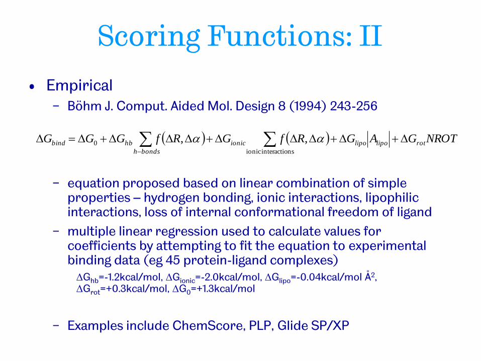
Scoring Functions: II
• Empirical − Böhm J. Comput. Aided Mol. Design 8 (1994) 243-256
− equation proposed based on linear combination of simple properties – hydrogen bonding, ionic interactions, lipophilic interactions, loss of internal conformational freedom of ligand
− multiple linear regression used to calculate values for coefficients by attempting to fit the equation to experimental binding data (eg 45 protein-ligand complexes)
Ghb=-1.2kcal/mol, Gionic=-2.0kcal/mol, Glipo=-0.04kcal/mol Å2, Grot=+0.3kcal/mol, G0=+1.3kcal/mol
− Examples include ChemScore, PLP, Glide SP/XP
NROTGAGRfGRfGGG rotlipolipoionic
bondsh
hbbind nsinteractioionic
0 ,,
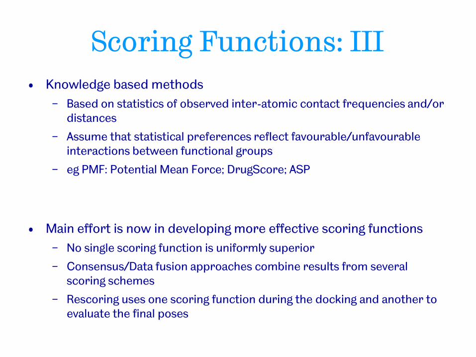
Scoring Functions: III
• Knowledge based methods
− Based on statistics of observed inter-atomic contact frequencies and/or distances
− Assume that statistical preferences reflect favourable/unfavourable interactions between functional groups
− eg PMF: Potential Mean Force; DrugScore; ASP
• Main effort is now in developing more effective scoring functions
− No single scoring function is uniformly superior
− Consensus/Data fusion approaches combine results from several scoring schemes
− Rescoring uses one scoring function during the docking and another to evaluate the final poses
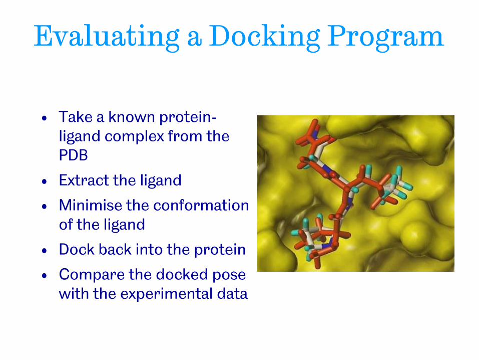
Evaluating a Docking Program
• Take a known protein-ligand complex from the PDB
• Extract the ligand
• Minimise the conformation of the ligand
• Dock back into the protein
• Compare the docked pose with the experimental data
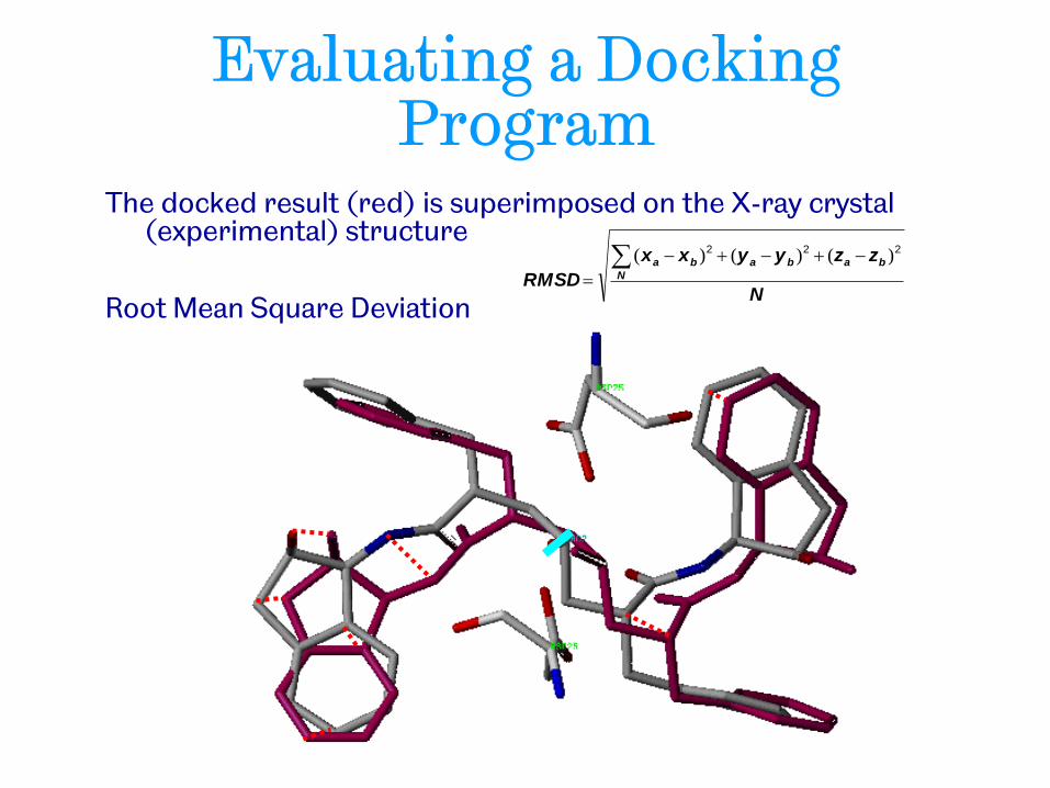
Evaluating a Docking Program
The docked result (red) is superimposed on the X-ray crystal (experimental) structure
Root Mean Square Deviation N
zzyyxx
RMSD N
bababa
222 )()()(
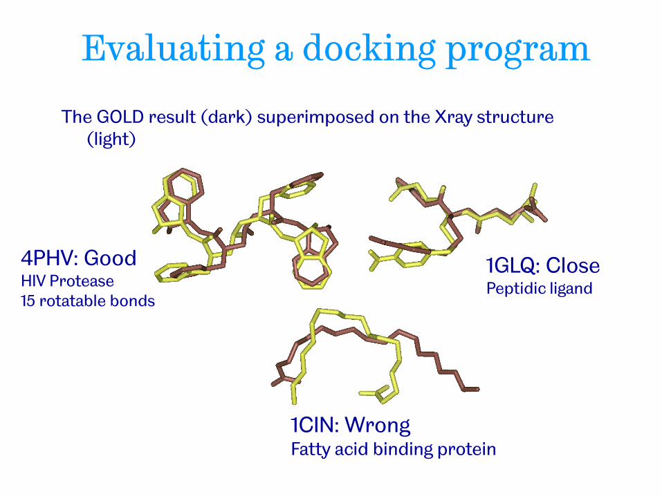
Evaluating a docking program
The GOLD result (dark) superimposed on the Xray structure (light)
4PHV: Good HIV Protease 15 rotatable bonds
1GLQ: Close Peptidic ligand
1CIN: Wrong Fatty acid binding protein
GOLD: Validation
• GOLD validation
− 305 complexes found in PDB (CCDC/Astex dataset)
− ligand extracted from complex
− ligand minimised
− docked back to protein
− GOLD prediction compared with original crystal structure
• ~72% success rate using stringent criteria
• G. Jones, P. Willett, R. C. Glen, A. R. Leach & R. Taylor, J. Mol. Biol 1997, 267, 727-748
• J. W. M. Nissink et al. “A New Test Set for Validating Predictions of Protein-Ligand Interaction”, Proteins 2002, 49, 457-471.
Issues related to the protein
• Need to ensure all residues are in the correct protonation and tautomeric states
• Protein conformation
− Can be several examples of the same protein but with different ligands bound
− The conformation of the binding site can vary from one complex to another
− Which should be used in the virtual screening experiment?
• Ensemble docking to different protein conformations may be required where there are large changes in the binding site

Where there’s no chicken wire, there are no electrons..atoms
An X-ray crystal structure is one crystallographer’s subjective interpretation of an observed electron-density map expressed in terms of an atomic models
A Davis, S Teague G Kleywegt Angew. Chem. 2003, 24, 2693
Homology models can be even more subjective

Issues related to the ligands
• The protonation state and tautomeric form of a ligand can influence its hydrogen bonding ability
− Need to ensure all ligands are in the correct protonation and tautomeric states or enumerate and dock all possibilities
• Conformations
− Need to ensure sufficient sampling of conformational space has been carried out
− Can we be sure the bioactive conformation has been generated?
− May want to apply filtering techniques to prune unlikely candidates prior to carrying out the docking
Enol Ketone
N
OH
NH
O
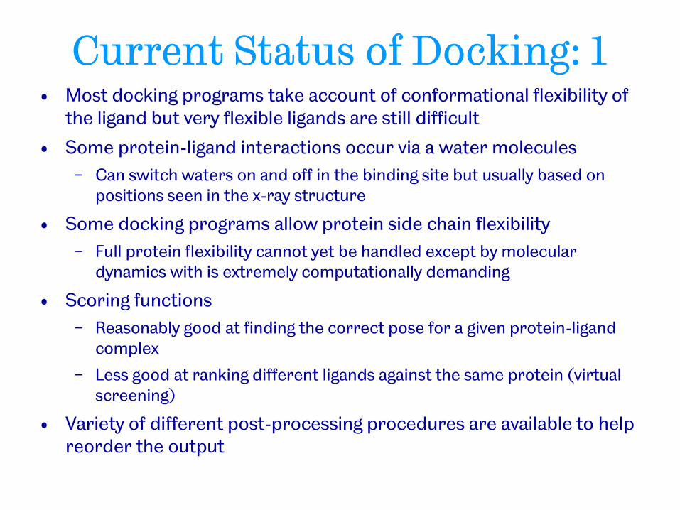
Current Status of Docking: 1 • Most docking programs take account of conformational flexibility of
the ligand but very flexible ligands are still difficult
• Some protein-ligand interactions occur via a water molecules
− Can switch waters on and off in the binding site but usually based on positions seen in the x-ray structure
• Some docking programs allow protein side chain flexibility
− Full protein flexibility cannot yet be handled except by molecular dynamics with is extremely computationally demanding
• Scoring functions
− Reasonably good at finding the correct pose for a given protein-ligand complex
− Less good at ranking different ligands against the same protein (virtual screening)
• Variety of different post-processing procedures are available to help reorder the output

Current Status of Docking: 2
• Despite its limitations docking is very widely used and there are many success stories
− see Kolb et al. Curr. Opin. Biotech., 2009, 20, 429, and Waszkowycz et al., WIREs Comp Mol. Sci., 2011, 1, 229)
• Performance varies from target to target, and scoring function to scoring function
− See for example, Plewczynski et al, “Can we trust docking results? Evaluation of seven commonly used programs on PDBbind database”, J. Comp. Chem., 2011, 32, 742.
• Care needs to be taken when preparing both the protein and the ligands
• The more information you have (and use!), the better your chances
− Targeted library, docking constraints, filtering poses, seeding with known actives, comparing with known crystal poses

Conclusions
• Wide range of virtual screening techniques have been developed
• The performance of different methods varies on different datasets
• Increased complexity in descriptors and method does not necessarily lead to greater success
• Combining different approaches can lead to improved results
• Computational filters should be applied to remove undesirable compounds from further consideration
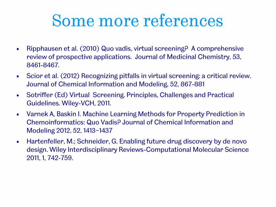
Some more references
• Ripphausen et al. (2010) Quo vadis, virtual screening? A comprehensive review of prospective applications. Journal of Medicinal Chemistry, 53, 8461-8467.
• Scior et al. (2012) Recognizing pitfalls in virtual screening: a critical review. Journal of Chemical Information and Modeling, 52, 867-881
• Sotriffer (Ed) Virtual Screening. Principles, Challenges and Practical Guidelines. Wiley-VCH, 2011.
• Varnek A, Baskin I. Machine Learning Methods for Property Prediction in Chemoinformatics: Quo Vadis? Journal of Chemical Information and Modeling 2012, 52, 1413−1437
• Hartenfeller, M.; Schneider, G. Enabling future drug discovery by de novo design. Wiley Interdisciplinary Reviews-Computational Molecular Science 2011, 1, 742-759.


![1 1 1 1 1 1 1 ¢ 1 , ¢ 1 1 1 , 1 1 1 1 ¡ 1 1 1 1 · 1 1 1 1 1 ] ð 1 1 w ï 1 x v w ^ 1 1 x w [ ^ \ w _ [ 1. 1 1 1 1 1 1 1 1 1 1 1 1 1 1 1 1 1 1 1 1 1 1 1 1 1 1 1 ð 1 ] û w ü](https://static.fdocuments.net/doc/165x107/5f40ff1754b8c6159c151d05/1-1-1-1-1-1-1-1-1-1-1-1-1-1-1-1-1-1-1-1-1-1-1-1-1-1-w-1-x-v.jpg)


![1 1 1 1 1 1 1 ¢ 1 1 1 - pdfs.semanticscholar.org€¦ · 1 1 1 [ v . ] v 1 1 ¢ 1 1 1 1 ý y þ ï 1 1 1 ð 1 1 1 1 1 x ...](https://static.fdocuments.net/doc/165x107/5f7bc722cb31ab243d422a20/1-1-1-1-1-1-1-1-1-1-pdfs-1-1-1-v-v-1-1-1-1-1-1-y-1-1-1-.jpg)