1 Unit III - WordPress.com · PROPAGATION OVER WATER OR FLAT OPEN AREA Propagation over water or...

CMC

Unit IIIPRESENTATION

BY

VIDYA SAGAR

1

Syllabus

CELL COVERAGE FOR SIGNAL AND TRAFFIC

Signal reflections in flat and hilly terrain, Effect of human made structures, Phase

difference between direct and reflected path, constant standard deviation, Straight line

path loss slope, General formula for mobile propagation over water and flat open area,

near and long distance propagation, Path loss from a point to point prediction model in

different conditions, merits of Lee model.

CELL SITE AND MOBILE ANTENNAS

Space diversity antennas, Umbrella pattern antennas, and minimum separation of cell site

antennas, mobile antennas.

CMC BY VIDYA SAGAR P 2-2

GENERAL INTRODUCTION

Cell coverage can be based on signal coverage or on traffic coverage.

We have to examine the service area as occurring in one of the following environments:

Human-made structures

In a building area

In an open area

In a suburban area

In an urban area

Natural terrains

Over flat terrain

Over hilly terrain

Over water

Through foliage areas


Ground Incident Angle and Ground Elevation Angle

A coordinate sketch in a flat terrain.


The ground incident angle θ is the angle of wave arrival incidentally pointing to the ground.

The ground elevation angle φ is the angle of wave arrival at the mobile unit.

Ground Reflection Angle and Reflection Point

A coordinate sketch in a hilly terrain.


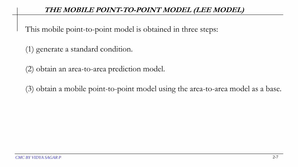
THE MOBILE POINT-TO-POINT MODEL (LEE MODEL)

This mobile point-to-point model is obtained in three steps:

(1) generate a standard condition.

(2) obtain an area-to-area prediction model.

(3) obtain a mobile point-to-point model using the area-to-area model as a base.


A Standard ConditionTo generate a standard condition and provide correction factors, we have used the

standard conditions shown on the left side and the correction factors on the right side of

TableGenerating a Standard Condition


Effect of the Human-Made Structures.

Because the terrain configuration of each city is different, and the human-made structure of

each city is also unique.

The way to factor out the effect due to the terrain configuration from the man-made

structures is to work out a way to obtain the path loss curve for the area.

The path loss curve obtained on virtually flat ground indicates the effects of the signal

loss due to solely human-made structures.


Propagation path loss curves for human-made structures.

(a) For selecting measurement areas

We may have to measure signal strengths at those high spots and also at the low spots surrounding the cell sites.


(b) path loss phenomenon.

Then the average path loss slope, which is a combination of measurements from high spots and

low spots along different radio paths in a general area, represents the signal received as if it is

from a flat area affected only by a different local human-made structured environment.


Therefore, the differences in area-to-area prediction curves are due to the different manmade

structures.

The measurements made in urban areas are different from those made in suburban and open areas.

Any area-to-area prediction model can be used as a first step toward achieving the point-to-point

prediction model.

Area-to-area prediction model which is described here can be represented by two parameters:

(1) the 1-mi (or 1-km) intercept point

(2) the path-loss slope.

The 1-mi intercept point is the power received at a distance of 1 mi from the transmitter.

There are two general approaches to finding the values of the two parameters experimentally.


(c) Propagation path loss in different cities.

1. Compare the area of interest with an area of similar human-made structures which presents a curve as shown.


2. If the human-made structures of a city are different from the cities listed in previous figure,

a simple measurement should be carried out.

Set up a transmitting antenna at the center of a general area.

As long as the building height is comparable to the others in the area, the antenna location is

not critical.

Take six or seven measured data points around the 1-mi intercept and around the 10-mi

boundary based on the high and low spots.

Then compute the average of the 1 mi data points and of the 10 mi data points.

By connecting the two values, the path-loss slope can be obtained.


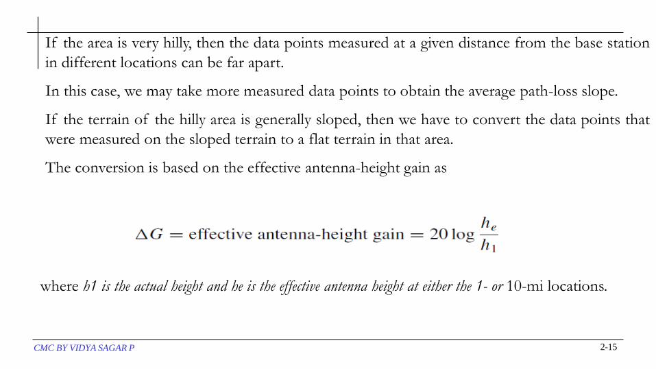
If the area is very hilly, then the data points measured at a given distance from the base station

in different locations can be far apart.

In this case, we may take more measured data points to obtain the average path-loss slope.

If the terrain of the hilly area is generally sloped, then we have to convert the data points that

were measured on the sloped terrain to a flat terrain in that area.

The conversion is based on the effective antenna-height gain as

where h1 is the actual height and he is the effective antenna height at either the 1- or 10-mi locations.


Path-loss Phenomena

The plotted curves shown in the previous figure have different 1-mi intercepts and different slopes.


(d) Explanation of the path-loss phenomenon.CMC BY VIDYA SAGAR P 2-17

The Phase Difference between a Direct Path and a Ground-Reflected Path

A simple model.


Based on a direct path and a ground-reflected path, where a direct path is a line-of-sight

(LOS) path with its received power

and a ground-reflected path with its reflection coefficient and phase changed after

reflection, the sum of the two wave paths can be expressed as:

where av = the reflection coefficient

φ = the phase difference between a direct path and a reflected path

P0 = the transmitted power

d = the distance

λ = the wavelength


In a mobile environment av = −1 because of the small incident angle of the ground wave

caused by a relatively low cell-site antenna height.

Thus,


Then the received power of becomes :

From Equation, we can deduce two relationships as follows:

If φ is less than 0.6 rad, then sin(φ/2) ≈ φ/2, cos(φ/2) ≈ 1 and equation simplifies to

where ΔP is the power difference in decibels between two different path lengths and ΔG is the gain

(or loss) in decibels obtained from two different antenna heights at the cell site.


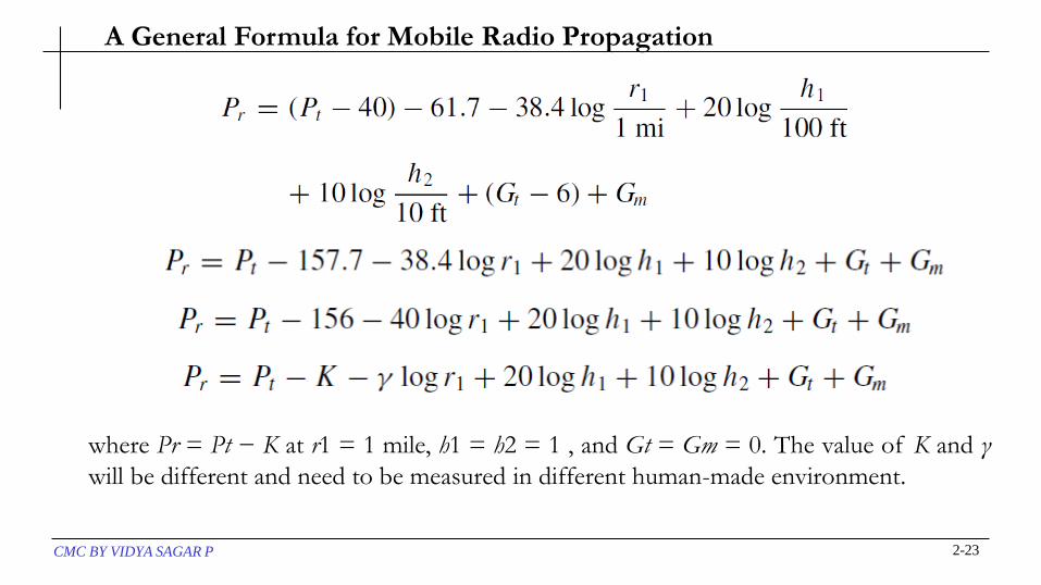
A General Formula for Mobile Radio Propagation

where Pr = Pt − K at r1 = 1 mile, h1 = h2 = 1 , and Gt = Gm = 0. The value of K and γ

will be different and need to be measured in different human-made environment.


PROPAGATION OVER WATER OR FLAT OPEN AREA

Propagation over water or flat open area is becoming a big concern because it is very easy

to interfere with other cells if we do not make the correct arrangements. Interference

resulting from propagation over the water can be controlled if we know the cause.

the permittivities of seawater and fresh water are the same, but the conductivities of seawater and

fresh water are different.

Then (seawater) = 80 − j84 and ( fresh water) = 80 − j0.021.

Based upon the reflection coefficients formula with a small incident angle,

both the reflection coefficients for horizontal polarized waves and vertically polarized

waves approach 1.

Because the 180◦ phase change occurs at the ground reflection point, the

reflection coefficient is −1.


A model for propagation over water.

Below shown are the two antennas, one at the cell site and the other at the mobile unit, are

well above sea level, two reflection points are generated.


The formula to find the field strength under the circumstances of a fixed point-to-point

transmission and a land-mobile transmission over a water or flat open land condition.

Between Fixed Stations

The point-to-point transmission between the fixed stations over the water or flat open

land can be estimated as follows. The received power Pr can be expressed as


Propagation between two fixed stations over water or flat open land.


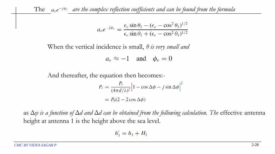
The are the complex reflection coefficients and can be found from the formula

When the vertical incidence is small, θ is very small and

And thereafter, the equation then becomes:-

as Δφ is a function of Δd and Δd can be obtained from the following calculation. The effective antenna

height at antenna 1 is the height above the sea level.


The effective antenna height at antenna 2 is the height above the sea level.

where h1 and h2 are actual heights and H1 and H2 are the heights of hills. In general, both antennas

at fixed stations are high, so the reflection point of the wave will be found toward the middle

of the radio path. The path difference d can be obtained as

Then, equation becomes


Therefore, we can set up five conditions:


Land-to-Mobile Transmission Over Water

There are always two equal-strength reflected waves, one from the water and one from the

proximity of the mobile unit, in addition to the direct wave.

Therefore, the reflected power of the two reflected waves can reach the mobile unit without

noticeable attenuation. The total received power at the mobile unit would be obtained by

summing three components.


Where Δφ1 and Δφ2 are the path-length difference between the direct wave and two reflected waves,

respectively. Because Δφ1 and Δφ2 are very small usually for the land-to-mobile path, then

Follow the same approximation for the land-to-mobile propagation over water.

Then,

In most practical cases, Δφ1 + Δφ2 < 1; then << 1 and the equation reduces to


FOLIAGE LOSS

Foliage loss is a very complicated topic that has many parameters and variations. The sizes

of leaves, branches, and trunks, the density and distribution of leaves, branches, and

trunks, and the height of the trees relative to the antenna heights will all be considered.

A characteristic of foliage environment.


This unique problem can become very complicated . For a system design, the estimate of the

signal reception due to foliage loss does not need any degree of accuracy.

Furthermore, some trees, such as maple or oak, lose their leaves in winter, while others, such

as pine, never do.

However, a rough estimate should be sufficient for the purpose of system design. In tropic

zones, the sizes of tree leaves are so large and thick that the signal can hardly penetrate.

Sometime the foliage loss can be treated as a wire-line loss, in decibels per foot or decibels per

meter, when the foliage is uniformly heavy and the path lengths are short.

When the path length is long and the foliage is non uniform, then decibels per octaves or

decibels per decade is used.


PROPAGATION IN NEAR-IN DISTANCE

We are using the suburban area as an example.

At the 1-mi intercept, the received level is −61.7 dBm based on the reference set of parameters;

that is, the antenna height is 30 m (100 ft).

If we increase the antenna height to 60 m (200 ft), a 6-dB gain is obtained. From 60 to 120

m (20 to 400-ft), another 6 dB is obtained.

At the 120-m (400-ft) antenna height, the mobile received signal is the same as that

received at the free space.

The antenna pattern is not isotropic in the vertical plane.


A typical 6-dB omni-directional antenna beam width.


The reduction in signal reception can be found in the figure and is listed in the table below.

At d = 100 m (328 ft) [mobile antenna height = 3 m (10 ft)], the incident angles and elevation angles

are 11.77◦ and 10.72◦, respectively.


Curves for near-in propagation.CMC BY VIDYA SAGAR P 2-38

Calculation of Near-Field Propagation

The range dF of near field can be obtained by letting φ in the equation below be π.

The signal received within the nearfield (d < dF ) uses the free space loss formula, and the signal

received outside the nearfield (d > dF ) can use the mobile radio path loss formula, for the best

approximation.


LONG-DISTANCE PROPAGATION

The advantage of a high cell site is that it covers the signal in a large area, especially in a

noise-limited system where usually different frequencies are repeatedly used in different

areas.

However, we have to be aware of the long-distance propagation phenomenon.

A noise-limited system gradually becomes an interference-limited system as the traffic

increases.

The interference is due to not only the existence of many co-channels and adjacent

channels in the system, but the long-distance propagation also affects the interference.

Within an Area of 50-mi Radius

For a high site, the low-atmospheric phenomenon would cause the ground wave path to

propagate in a non-straight-line fashion.

The wave path can bend either upward or downward.

Then we may have the experience that at one spot the signal may be strong at one time but

weak at another.CMC BY VIDYA SAGAR P 2-40

At a Distance of 320 km (200 mi)

Tropospheric wave propagation prevails at 800 MHz for long-distance

propagation; sometimes the signal can reach 320 km (200 mi) away.

The wave is received 320 km away because of an abrupt change in the effective

dielectric constant of the troposphere.

The dielectric constant changes with temperature, which decreases with height at a

rate of about 6.5◦C/km and reaches −50◦C at the upper boundary of the

troposphere.

In tropospheric propagation, the wave may be divided by refraction and reflection.

Tropospheric refraction: This refraction is a gradual bending of the rays due to

the changing effective dielectric constant of the atmosphere through which the

wave is passing.


Tropospheric reflection: This reflection will occur where there are abrupt changes in the

dielectric constant of the atmosphere. The distance of propagation is much greater than

the line-of-sight propagation.

Moistness: Water content has much more effect than temperature on the dielectric

constant of the atmosphere and on the manner in which the radio waves are affected.

The water vapor pressure decreases as the height increases.

Tropospheric wave propagation does cause interference and can only be reduced by

umbrella antenna beam patterns, a directional antenna pattern, or a low-power low-antenna

approach.


General Formula of Lee Model

Lee’s point-to-point model has been described. The formula of the Lee model can be stated

simply in three cases:

1. Direct-wave case. The effective antenna height is a major factor which varies with the

location of the mobile unit while it travels.

2. Shadow case. No effective antenna height exists. The loss is totally due to the knife-edge

diffraction loss.

3. Over-the-water condition. The free space path-loss is applied.


• An antenna is a device used to transform an RF signal, traveling on aconductor, into an electromagnetic wave in free space.

• The first antennas were built in 1888 by German physicist HeinrichHertz in his pioneering experiments to prove the existence ofelectromagnetic waves predicted by the theory of James ClerkMaxwell.

Typically an antenna consists of an arrangement of metallicconductors (“elements"), electrically connected (often through atransmission line) to the receiver or transmitter.

• Antennas are reciprocal, i.e. the same design works for receivingsystems as for transmitting systems. 3

Introduction

• Ideally all incident energy must be reflected back when open circuit.

• But practically a small portion of electromagnetic energy escapes from thesystem that is it gets radiated.

• The amount of escaped energy is very small due to mismatch betweentransmission line and surrounding space.

• Also because two wires are too close to each other, radiation from one tip willcancel radiation from other tip.( as they are of opposite polarities and distancebetween them is too small as compared to wavelength )

G

Radiation Mechanism

• To increase amount of radiated power open circuit must beenlarged , by spreading the two wires.

• Due to this arrangement, coupling between transmission line andfree space is improved.

• Also amount of cancellation has reduced.

• The radiation efficiency will increase further if two conductorsof transmission line are bent so as to bring them in same line.

47

Radiation Mechanism..

• According to their applications and technology available, antennas generallyfall in one of two categories:

• 1.Omnidirectional or only weakly directional antennas which receive orradiate more or less in all directions.

• These are employed when the relative position of the other station is unknown orarbitrary.

• They are also used at lower frequencies where a directional antenna would be toolarge, or simply to cut costs in applications where a directional antenna isn'trequired.

• 2. Directional or beam antennas which are intended to preferentiallyradiate or receive in a particular direction or directional pattern.

AntennaTypes

• According to length of transmission lines available, antennasgenerally fall in one of two categories:

• 1. Resonant Antennas – is a transmission line, the length of whichis exactly equal to multiples of half wavelength and it is open atboth ends.

• 2. Non-resonant Antennas – the length of these antennas isnot equal to exact multiples of half wavelength.

• In these antennas standing waves are not present as antennas areterminated in correct impedance which avoid reflections.

• The waves travel only in forward direction.

• Non-resonant antenna is a unidirectional antenna.

AntennaTypes..

• Radiation Resistance

• This relates the power supplied to the antenna and the current flowing into theantenna.

• The greater the radiation resistance, the more energy is radiated or received bythe antenna.

• To optimize an antenna system, this resistance should match the resistance of thetransmitter or receiver system.

8

AntennaPrincipals

•Antenna Pattern•This shows a distribution of radiated power

as a function of direction in space.

•Typically displayed in a polar plot.

•This example shows an antenna that

radiates a lot of power in one direction but

very little in other directions.

EQUIVALENT CIRCUIT OF ANTENNAS:

The operating conditions of an actual antenna (Fig.) can be expressed in

an equivalent circuit for both receiving (Fig b) and transmitting (Fig.c). In

Fig. 3.9, Za is the antenna impedance; Zl is the load impedance, and Zt is

the impedance at the transmitter terminal.

From the transmitting end (obtaining free-space path-loss formula):

Power Pt originates at a transmitting antenna and radiate out into space.

(Equivalent circuit of a transmitting antenna is shown in Fig.3.9b.)

Assume that an isotropic source Pt is used and that the power in the

spherical space will be measured as the power per unit area. Thus power

density, called the Poynting vector p or the outward flow of

electromagnetic energy through a given surface area, is expressed as

Fig.3.9 (a) An actual antenna ;(b) equivalent circuit of transmitting antenna;

(c) equivalent circuit of a receiving antenna

• Directivity and Gain• The directivity and gain are related parameters; the directivity measures theantenna’s ability to concentrate its power in a given direction and the gain is theratio of power radiated to input power.

• Bandwidth• The bandwidth of an antenna refers to the frequencies available outside the center

frequency.• For example, a 10MHz transmitter with 10% bandwidth could send

information on frequencies from 9 MHz to 11Mhz.• Beam-width

• Beam-width of an antenna is defined asangular separation between the two half power pointson power density radiation pattern.

OR• Angular separation between two 3dB

down points on the field strength of radiation pattern.9•

It is expressed in degrees.

• Isotropic (Reference)

• The Isotropic Radiator would radiate all the power delivered to itand equally in all directions

• The isotropic radiator would also be a point source.

• The Half-Wave Dipole

• The total length of the antenna is equal to half of the wavelength ofthe signal you’re trying to transmit or receive.

• The dipole is fed by a two wire line where the two currents are equalin amplitude but opposite in direction.

• The ends are essentially an open circuit, so most of the energy isradiated out the center of the antenna.

• The electric field radiates in a donut shaped pattern around thedipole axis, and the magnetic field radiates in a circle outward fromthe antenna.

• The quarter-wave Monopole• It is very similar to the above type.

• It basically consists of one-half a dipole plus a perfectly conducting plane.

10

CommonAntennaTypes

• Loop Antennas

• Microstrip Antennas

• Horn Antennas

• Helical Antennas

• Dish Antennas11

CommonAntennaTypes..

• Mobile and portable antennas usedwith cellular and PCS systems haveto be omnidirectional and small.

• The simplest antenna is the quarter-wavelength monopole these areusually the ones supplied withportable phones.

• For mobile phones, and commonconfiguration is the quarter-waveantenna with a half-wave antennamounted above it.

Mobileand PortableAntenna

• Cell site is used to refer to the physical location of radioequipment that provides coverage within a cell.

• For cellular radio systems, there is a need for omnidirectionalantennas and for antennas with beamwidths of 120º, and less forsectorized cells.

• Cellular and PCS base-station receiving antennas are usuallymounted in such a way as to obtain space diversity.

• For an omnidirectional pattern, typically three antennas are mountedon a tower with a triangular cross section and the antennas aremounted at 120º intervals.

Cell SiteAntennas

ANTENNAS AT CELL SITE

• For Coverage

– Use Omni-directional Antennas

• High-Gain Antennas

• There are standard 6-dB and 9-dB gain omni-directional antennas

High-gain omnidirectional antennasGain with reference to dipole: (a) 6 dB; (b) 9 dB

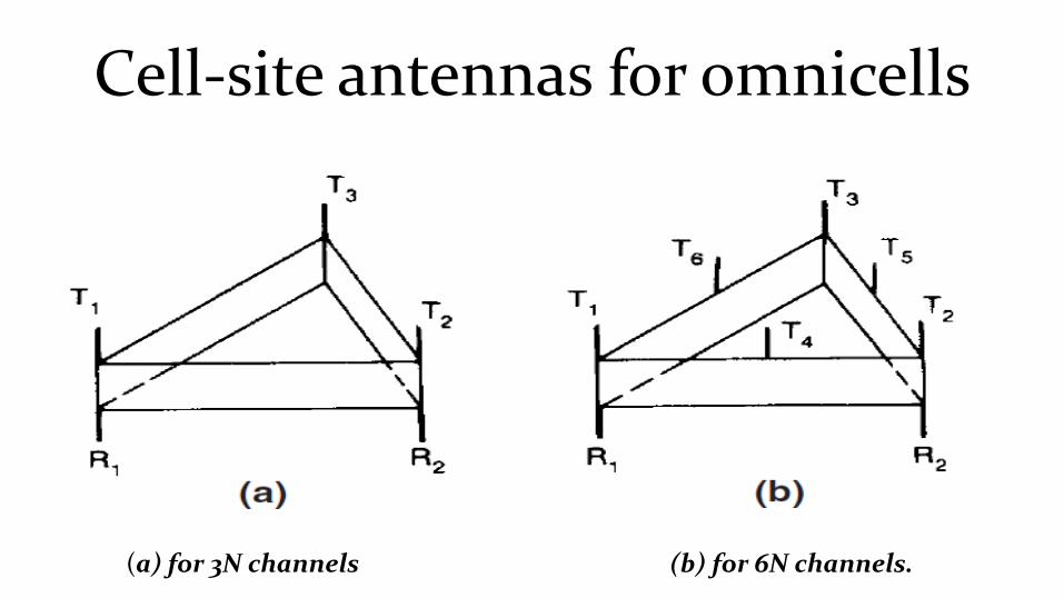
Cell-site antennas for omnicells

(a) for 3N channels (b) for 6N channels.

Ring combiner• A ring combiner is used to combine two

groups of channels into a single output.

• The function of a ring combiner is tocombine two 16-channel combiners intoone 32-channel output.

• Therefore, all 32 channels can be used bya single transmitting antenna.

• The ring combiner has a limitation ofhandling power up to 600 W with a lossof 3 dB.

Relation between Gain and Beam Width

• Relation between Gain and Beam Width• The receiver gain GR can be related to its half-power

beam width as

• θHP and φHP are the half-power beam widths in the θ and φ planes

• The factor 4π is the solid angle subtended by a sphere in steradians (square radians)

Relation between Gain and Beam Width

A typical pattern for a directional antenna of 120° beamwidth

(a) Azimuthal pattern of8-dB directional antenna

A typical pattern for a directional antenna of 120° beamwidth

(b) Vertical pattern of8-dB directional antenna

Directional antenna arrangement

(a) 120◦ sector (45 radios);(b) 60◦ sector; (c) 120◦ sector (90 radios).

Cell-site antenna mounting

Other Antennas at cellsite

• Location antennas

• Setup channel antennas

• Spaced diversity antennas

Spatial Diversity

Diversity Antenna Spacing

(a)η = h/d; (b)(b) proper arrangement with two antennas.

Umbrella-Pattern Antennas

• Normal Umbrella-Pattern Antenna.

• Broadband Umbrella-Pattern Antenna

• High-Gain Broadband Umbrella-Pattern Antenna

Dipole antenna

Monopole Antenna

Discone Antennas

(a)Single antenna. (b) An array of antennas

Photo of discone antenna

Discone Antenna

Radiation pattern

High gain Broadband umbrella-pattern antenna

UNIQUE SITUATIONS OF CELL-SITE ANTENNAS

Antenna Pattern in Free Space and in Mobile Environments

Front-to-back ratio of a directional antenna in amobile radio environment.

Minimum Separation of Cell-Site Receiving Antennas

Antenna pattern ripple effect

• The greater the antenna separation, theless likely the fades of the two receivedsignals will occur simultaneously.

• Thus the diversity gain for reducing theeffect of the

• fades increases as the separation increases.• Two types of separation:• Horizontal (shown in figure).• Vertical.• Separation distance depends on the

antenna height.

By experiments, optimum

MOBILE ANTENNAS

• Roof-Mounted Antenna

• Glass-Mounted Antennas

Mobile antenna patterns

(a) Roofmounted3-dB-gain collinear antennaversus roof-mountedquarter-wave antenna.

Mobile antenna patterns(b) Windowmounted“on-glass” gain antennaversus roof-mountedquarter-wave antenna.

Roof Mounted Antenna

Mobile Antennas

• Mobile High-Gain Antennas

• Horizontally Oriented Space-Diversity Antennas

• Vertically Oriented Space-Diversity Antennas

Horizontally spaced antennas

(a) Maximum difference in lcr of a four-branch equal-gain signal between α = 0 and α = 90◦ with antenna spacing of 0.15λ (b) Not recommended. (c) Recommended.

Vertical separation between two mobile antennas.

The theoretical derivation of correlation

Correlation coefficients in different areas and different street orientations.

Two vertically spaced

antennas mounted on

a mobile unit.

Thank you………………92

1 Unit III - WordPress.com · PROPAGATION OVER WATER OR FLAT OPEN AREA Propagation over water or...

Documents

Transcript of 1 Unit III - WordPress.com · PROPAGATION OVER WATER OR FLAT OPEN AREA Propagation over water or...