1. The inﬁnite square well - Queen's University Belfast · 1. The inﬁnite square well ... even...

PHY3011 Wells and Barriers page 1 of 17

1. The infinite square well

First we will revise the infinite square well which you did at level 2. Instead of thewell extending from 0 to a, in all of the following sections we will use a well that extendsfrom −a to a, that is, twice as wide and centred at 0. Of course the solutions are thesame: they’re just shifted and scaled (see Robinett, chapter 5).

The potential is

V (x) ={

0, for − a ≤ x ≤ a,∞, for |x| > a,

Outside the well where the potential is infinite there is no probability for the particle tobe found and so ψ(x) = 0 for |x| > a. Inside the well the potential is zero so the timeindependent Schrodinger equation reads

− h2

2md2ψdx2

= Eψ

which we writed2ψdx2

= −k2ψ

and

k =1h

√

2mE

There are no normalisable solutions for E < 0 and so k is real and the general solution is

ψ(x) = A sinkx+B coskx

The boundary conditions areψ(−a) = ψ(a) = 0

soA sinka+B coska = 0

−A sinka+B coska = 0

Adding or subtracting these we get either

A sinka = 0 or B coska = 0

Because the potential has inversion symmetry, V (−x) = V (x), it is natural that thesolutions fall into two classes: even parity solutions having ψ(−x) = ψ(x), and odd parity

solutions having ψ(−x) = −ψ(x). And the two possible boundary conditions give rise toone of these sets each. Specifically since we cannot have both A and B equal to zero(since then ψ = 0 everywhere and this cannot be normalised) the two sets correspondrespectively to either A = 0 or B = 0.

The boundary condition A = 0 leads to the even parity solutions. In this case we havecoska = 0 which is true if

k = kem =(

m− 1

2

)

πa

=(2m− 1)π

2a, m = 1,2,3, · · ·

and the eigenfunctions of the even solutions are

ψm(x) = B coskemx


The other case, B = 0 leads to the odd parity solutions with boundary condition A sinka =0 implying

k = kom =mπa

=2mπ2a

, m= 1,2,3, · · ·

with eigenfunctionsψm(x) = A sinkomx

We note that the eigenfunctions can be written as

ψn(x) ={

C cosknx, n = 2m− 1 i.e., n oddC sinknx n = 2m i.e., n even

andkn =

nπ2a, n = 1,2,3, · · ·

The boundary condition fixes the allowed wavelength λn = 2π/kn. kn is called a quantum

number and generally speaking quantum numbers arise as labels which dictate the allowedsolutions under the given boundary conditions. The allowed energies are the eigenvalues

associated with the values of kn. Since we will have kn =√

2mEn/h it follows that

En =h2k2

n2m

=n2π2 h2

2m(2a)2

To find the constant C, we normalise the wavefunction.

∫ a

−a

∣

∣C∣

∣

2cos2 kx dx=

∫ a

−a

∣

∣C∣

∣

2sin2 kx dx = a

∣

∣C∣

∣

2= 1

and so we can take C = 1/√a.

Please note that these ψn(x) are eigenvectors. A stationary state of the infinite squarewell is

Ψn(x, t) = ψn eiEnt/h

Now comes an important point. The eigenvectors

ψn(x) = |n〉

provide a basis in which to express any wavefunction that satisfies the boundary conditionslaid down by the potential (in this case the infinite square well) just like the basis vectors

ı , and k are a basis for any cartesian vector. Mathematically we can write the state ofany particle in the infinite square well as a linear combination

ψ(x) =∞∑

n=1

cnψn(x)

=∞∑

n=1

cn |n〉

(In the second line I have used the vector notation to describe the eigenvector.) Unlikecartesian space, this space is infinite dimensional. It’s exactly the same as Fourier analysiswhich says that any function in some interval, which is zero at the ends, can be expandedin sines and cosines having the same boundary conditions. Using Fourier analysis we find


the important result that the coefficients cn in the expansion above can be found usingan integral,

cn =∫ a

−aψ∗

n(x)ψ(x)dx

= 〈n∣

∣ψ⟩

And, again, I have indicated the alternative vector notation that emphasises this as ascalar product between the state and one of the eigenstates. Another property of thebasis functions is that they are orthonormal,

∫ a

−aψ∗

m(x)ψn(x) dx = δmn

〈m |n〉 = δmn

where δmn is the “Kronecker delta,” it’s zero if m 6= n and one if m = n. The fact thatthe scalar product between two eigenstates is zero unless they are identical is completelyanalogous to the orthogonality between the cartesian unit vectors, ı , and k . For example

· k = 0

butı · ı = 1

This will become a lot clearer when I do an example in class.


2. The finite square well

The potential is

V (x) ={−V0, for − a ≤ x ≤ a,

0, for |x| > a,

with V0 > 0. We first consider states with energy E < 0. Classically they would beconfined within the well. In quantum mechanics a particle is represented by a solutionto the time independent Schrodinger equation. The strategy is to find solutions in thethree regions, left of the well, in the well and right of the well. To the left, x < −a, thepotential is zero and we have

− h2

2md2ψdx2

= Eψ

which we writed2ψdx2

= κ2ψ (1a)

with

κ =1h

√

−2mE (1b)

The general solution isψ(x) = Ae−κx +Beκx

but we must have A = 0 or this blows up at large negative x.Inside the well the time independent Schrodinger equation reads

− h2

2md2ψ

dx2− V0ψ = Eψ

which we writed2ψ

dx2= −l2ψ (2a)

with

l =1h

√

2m(E + V0) (2b)

While E < 0 it’s also true that E > −V0 because there is no normalisable solution in thewell for energy less than −V0 (why not?). Please note the signs on κ and l on the righthand sides of (1a) and (2a). Solutions of equations like (1a) with positive coefficent arealways exponentially decaying, like e±κx, while if the coefficient is negative as in (2a) thesolution is oscillatory like e±ilx which we can also equally correctly write in terms of sinesand cosines:

ψ(x) = C sin lx+D cos lx

Note it is conventional to use the symbols k or l for the quantum number in the oscillatorycase and to use the symbol κ in the decaying case. In your level 2 notes you used α ratherthan κ as I shall also do in handwritten notes, since k and κ look very similar.

To the right of the well the potential is again zero and the energy of the state is lessthan this so the particle is classically forbidden this region. The signature of this is anexponentially decaying wavefunction just as to the left of the well. So for x > a we have

ψ(x) = Fe−κx


The procedure is one we will use in all problems of this type. First we write down thewavefunction and its first derivative with respect to x in the three regions.

ψ(x) =

Beκx, for x < −aC sin lx+D cos lx, for − a ≤ x ≤ a,Fe−κx, for x > a

ψ′(x) =

κBeκx, for x < −alC cos lx− lD sin lx, for − a ≤ x ≤ a,−κFe−κx, for x > a

The task at hand is to find those values of the constants B, C, D and F that render thewavefunction continuous and differentiable over the whole range of x. I will show laterfor the case of states with E > 0 how this is done in a general way. We approach thisparticular problem, E < 0, in a way that exploits the symmetry of the potential, namelythat it is symmetrical about x = 0 so that the wavefunction solutions must be either ofeven parity (ψ(x) = ψ(−x)) or of odd parity (ψ(x) = −ψ(−x)). We then seek first theeven solutions and then the odd solutions. For the even solutions we have

ψ(x) =

ψ(−x), for x < −aD cos lx, for − a ≤ x ≤ a,Fe−κx, for x > a

For ψ to be continuous at x= a we must have

Fe−κa =D cos la

and to be differentiable we need

−κFe−κa = −lD sin la

Dividing these two equations one by the other we get

κ = l tan la even solutions (3)

and this is the answer. Looking at (1b) and (2b) you see that the allowed energies, E,are those which result in κ and l obeying (3). For each allowed energy, we get κ and lwhich we plug into the wavefunctions in the three regions. At the same time we can solvefor the constants F and D (one of which is arbitrary and can be chosen to normalise thewavefunction over the range of x).

Now, for the odd solutions we write

ψ(x) =

−ψ(−x), for x < −aC sin lx, for − a ≤ x ≤ a,Fe−κx, for x > a

and matching value and slope at x = a results in

ψ(a) = Fe−κa = C sin la

ψ′(a) = −κFeκa = lC cos la


which when we divide one by the other, we arrive at

−κ=l

tan laodd solutions (4)

Equations (3) and (4) do not have analytical solutions but we can find the answers graph-ically or by computation. To do this we define some dimensionless parameters,

z = la, and z0 =ah

√

2mV0

and (3) and (4) become, in terms of z and z0

tan z =

[

(z0/z)2 − 1

]1/2, even solutions

[

(z0/z)2 − 1

]−1/2, odd solutions

π 2π 3π 4π 5π

even solutions

odd solutions

z0=16

z0=8

z0=16z0=8

To find even and odd solutions we just have to plot tanz against the right hand sides.The figure shows this plot for two cases, z0 = 8 and z0 = 16. Note that z0 is proportionalto the width and the square root of the depth of the well; it therefore is a measure of the“strength” of the potential well. From (2b) we have

En + V0 =h2l2

2m= z2

h2

2ma2


In the case of a very deep well, we see from the figure that the intersections occurnear the infinities of tan z, namely

zn → nπ/2 as z0 → ∞and so in the limit of an infinitely deep well we get that the eigenenergies measured fromthe bottom of the well, −V0 are

n2π2 h2

2m(2a)2

which are of course the energies of a particle trapped in an infinite square well of width2a.

In the other limit, as z0 → 0, we see from the figure that there are fewer and fewerstates “bound by the potential” and for z0 < π/2 there are no odd states and just oneeven state. It is significant that this survives however weak is the potential: even theweakest and narrowest square well will bind at least one state.

The next figure shows this lowest energy bound state and also the second and sixthstates, which are odd and even respectively, for z0 = 16. These have the shapes of thestates of the infinite square well, but unlike classical particles, the quantum mechanicsadmits a non zero probability that a measurement will find the particle outside the wallseven though its energy is less than zero. I also show the eigenvalues of the first 10 boundstates. You note that the probability density of a measurement finding the particle outside

the well increases with the quantum number n. You might think this is inconsistent withBohr’s correspondence principle which asserts that the classical limit corresponds to largerquantum numbers; but in this case the increased probability is due to the energy gettingcloser to zero after which the states and are free from the well altogether. These states,having E < 0, are discussed next.


So those were the particles whose energies were below zero so that they are trappedin or near the well. Now we come to particles whose energies are greater than zero so theycan exist as propagating stationary states anywhere in the range of x (−∞< x <∞).

I will do this using the general method of “transfer matrices.” First we write downthe wavefunctions and derivatives in the three regions as before.

ψ(x) =

Aeikx +Be−ikx, for x < −aC sin lx+D cos lx, for − a ≤ x ≤ a,Feikx +Ge−ikx, for x > a

ψ′(x) =

ikAeikx − ikBe−ikx, for x < −alC cos lx− lD sin lx, for − a ≤ x ≤ a,ikFeikx − ikGe−ikx, for x > a

in which

k =1h

√

2mE

and

l =1h

√

2m(E + V0)

In the well the wavefunction is the same as in the bound state, but outside the well thereare now running wave solutions travelling left (e−ikx) and right (eikx). We need to jointhe three regions up by matching value and slope at the boundaries of the well as before.So at x= −a we have

Ae−ika +Beika = −C sin la+D cos la

ikAe−ika − ikBeika = lC cos la+ lD sin la (5a)

and at x= a

C sin la+D cos la = Feika +Ge−ika

lC cos la− lD sin la = ikFeika − ikGe−ika (6a)

Now the nub. We can solve these as simultaneous equations bit by bit as we did forthe bound states by adding and subtracting. But you know that you can usually solvesimultaneous equations with matrices. So inspecting these sets of equations for a momentyou see they are equivalent to these:

(

e−ika eika

ike−ika −ikeika

)(

AB

)

=(

− sin la cos lal cos la l sin la

)(

CD

)

(5b)

(

sin la cos lal cos la −l sin la

)(

CD

)

=(

eika e−ika

ikeika −ike−ika

)(

FG

)

(6b)

Remember the quantum numbers k and l are fixed by the energy E for which we areseeking a solution. What we want are the coefficients A, B, C and D to plug back intothe wavefunction. Before doing that let’s just look at the physics of this problem. We maywell be asking, suppose I launch a wave in from the left at the well. How much probabilityamplitude is transmitted and how much is reflected? Then I will fix A from the outset bythe normalisation of the incoming wave. The amplitude A tells me how much is reflected


and the amplitude F how much is transmitted. As long as I don’t expect any amplitudecoming in from the right (it’s my experiment after all) then I may take it that G = 0.

The next figure shows such a matched solution for an energy just above zero, E =0.1V0,

Re ψIm ψamplitude

E

Anticipating ahead, what I really want to know is the transmission coefficient

T =

∣

∣F∣

∣

2

∣

∣A∣

∣

2

In the meanwhile I may want to know what is the wavefunction in the well, so I’ll wantto know C and D as well.

I will rewrite (5b) and (6b) like this

M1

(

AB

)

=M2

(

CD

)

(5c)

M3

(

CD

)

=M4

(

FG

)

(6c)

I can multiply (5c) by the inverse of M1 and (6c) by the inverse of M3. Then I substitute(6c) into (5c) and I get

(

AB

)

=M−11 M2M

−13 M4

(

FG

)

= P(

FG

)

and P is called the transfer matrix. This is a very general way to deduce the relationbetween waves going in and waves coming out of a one dimensional scattering problem.


There may be more than one well or barrier one after the other and this is the way totackle such a problem.

For these purposes we just need to solve for A and B in terms of C and D and forC and D in terms of F and G and finally to get all the coefficients so we can plot thewavefunction and extract the transmission coefficient. So firstly I have

(

AB

)

=M−11 M2

(

CD

)

(7)

It’s useful to remember how to invert a 2× 2 matrix.

if T =(

a bc d

)

then T−1 =1

ad− bc

(

d −b−c a

)

(Multiply by one over the determinant, swap the diagonals and change the sign of the offdiagonals.) We’ll get

M−11 M2 =

i2k

(

−ikeika −eika

−ike−ika e−ika

)(

− sin la cos lal cos la l sin la

)

=i

2k

(

eika (ik sin la− l cos la) −eika (ik cos la+ l sin la)e−ika (ik sin la+ l cos la) e−ika (−ik cos la+ l sin la)

)

Putting this in (7) you’ll find

A =i

2keika

(

C (ik sin la− l cos la) −D (ik cos la+ l sin la))

B =i

2ke−ika

(

C (ik sin la+ l cos la) +D (−ik cos la+ l sin la))

Next we do the same thing with (6c). But we’ll now set G = 0 as discussed above, andto keep the algebra simpler. (If there were amplitude coming in from the right also, thenyou can retain G 6= 0.)

M−13 M4 =

1l

(

l sin la cos lal cos la − sin la

)(

eika e−ika

ikeika −ike−ika

)

=1l

(

eika (l sin la+ ik cos la) e−ika (l sin la− ik cos la)eika (l cos la− ik sin la) e−ika (l cos la+ ik sin la)

)

and (6c) becomes

C = Feika(

sin la+ ikl

cos la)

D = Feika(

cos la− ikl

sin la)

Finally I substitute these into my formulas for A and B to get A and B in terms of F . Ifind after quite a bit of algebra

B =iF2kl

(

l2 − k2)

sin2la

A = Fe2ika

(

cos2la− i l2 + k2

2klsin2la

)


So the transmission coefficient must be given by

T−1 =

∣

∣A∣

∣

2

∣

∣F∣

∣

2= 1 +

V 20

4E(E + V0)sin2

(

2ah

√

2m(E + V0))

(8)

The next figure shows the transmission coefficient plotted versus the energy (rememberthis is the energy above the top of the well). If the energy is less than zero there are notravelling solutions outside the well, the particle is trapped inside although it can tunnelto the outside as seen in the figure on page 6. Note that the figure below plots the samefunction twice over, in different ranges of the energy.

0 10 20 30 40 500.98

1

E / V0

tran

smis

sion

0 1 2 3 4 50

0.25

0.5

0.75

1

E / V0

tran

smis

sion

square well

You notice that the transmission coefficient periodically becomes one as a function ofthe energy of the incoming wave. This happens as you see from equation (8) wheneverthe sine is zero. That is, when

2ah

√

2m(E + V0) = nπ

for any integer n. So there is perfect transmission (no reflection) whenever

E + V0 =n2π2 h2

2m(2a)2= En

but these are the energy eigenvalues of the infinite square well, measured from the bottomof the well. This is a quite remarkable fact.


3. The square barrier

The square barrier rises above the zero of energy having a constant potential V0between −a < x < a. If we look for energies greater than V0 then the problem is the sameas for the finite well as you can see from the following figure.

−V0

V0

E

0

As long as E > V0 then the problem is the same as for the well having E > 0, exceptthat the kinetic energy in the barrier is E − V0 rather than E + V0. So the solution isexactly as for the well except that now

l =1h

√

2m(E − V0)

This means that wavefunctions approaching the barrier are reflected and transmitted witha transmission coefficient given by equation (8) with the sign of V0 changed,

T−1 = 1 +V 2

04E(E − V0)

sin2(

2ah

√

2m(E − V0))

(9)

A classical particle would also fly over the barrier, but what if the energy is less thanV0? This is the most interesting case; classically a particle would bounce off the barrier,but in quantum mechanics there’s a finite probability for the particle to “tunnel” throughthe barrier and appear on the other side.

Re ψIm ψamplitude

E


The figure above shows tunnelling of a particle with energy E = 0.1V0 which youcan compare with the figure on page 9. In either case, the amplitude is constant on theright as there is only an outgoing wave and this must have a constant intensity, or energyis not conserved. On the left on the other hand what you see is interference betweenthe incoming and reflected waves, and the combination has a varying amplitude. In thetunnelling case note how the wavefunction is decaying in the barrier and what remains isallowed to “leak out into the vacuum” and propagate.

The transmission coefficient in the tunnelling case, E < V0, as compared to equa-tion (9) is given by

T−1 = 1 +V 2

04E(V0 −E)

sinh2(

2ah

√

2m(V0 −E))

(10)

I’ll now derive this result (you may skip this bit) using the method of transmission ma-trices. It’s almost the same as the case of the potential well. The wavefunction is

ψ(x) =

Aeikx +Be−ikx, for x < −aCelx +De−lx, for − a ≤ x ≤ a,Feikx +Ge−ikx, for x > a

The only difference is that inside the well the wavefunctions are decaying—it’s like thecase of states bound within a finite well that decay to the outside. These now decay tothe inside. The slopes are

ψ′(x) =

ikAeikx − ikBe−ikx, for x < −alCelx − lDe−lx, for − a ≤ x ≤ a,ikFeikx − ikGe−ikx, for x > a

in which

k =1h

√

2mE

and

l =1h

√

2m(V0 −E)

At x= −aAe−ika +Beika = Ce−la +Dela

ikAe−ika − ikBeika = lCe−la − lDela

and at x= aCela +De−la = Feika +Ge−ika

lCela − lDe−la = ikFeika − ikGe−ika

(

e−ika eika

ike−ika −ikeika

)(

AB

)

=(

e−la ela

le−la −lela)(

CD

)

(

ela e−la

lela −le−la

)(

CD

)

=(

eika e−ika

ikeika −ike−ika

)(

FG

)

By solving these matrix equations in the same way as before you will get these expressionsfor A and B in terms of C and D,

A =i

2keika

(

−Ce−la (l+ ik) +Dela (l − ik))

B =i

2ke−ika

(

Ce−la (l − ik) −Dela (l+ ik))


and solving for C and D in terms of F (again we set G = 0)

C =F2leika

(

e−la (l+ ik))

D =F2leika

(

ela (l − ik))

Then

A =iF4lk

(

−e2(ik−l)a (l+ ik)2+ e2(ik+l)a (l − ik)2

)

=iF4lk

e2ika(

−e−2la(

l2 − k2 + 2ilk)

+ e2la(

l2 − k2 − 2ilk))

=iF4lk

e2ika((

e2la − e−2la)(

l2 − k2)

−(

e2la + e−2la)

2ilk)

= Fe2ika

(

cosh 2la+ il2 − k2

2lksinh 2la

)

so finally forming |A|2/|F |2 we get the inverse of the transmission coefficient

T−1 = 1 +V 2

04E(V0 −E)

sinh2(

2ah

√

2m(V0 −E))

(10)

0 10 20 30 40 500.98

1

E / V0

tran

smis

sion

0 1 2 3 4 50

0.25

0.5

0.75

1

E / V0

tran

smis

sion

square barrier

The figure above shows equations (9) and (10) which is the transmission coefficient ofthe barrier for energies below the barrier (10) left of the dotted line; and above (9) rightof the dotted line.


Again we see perfect transmission when the sine in (9) is zero, that is

2ah

√

2m(E − V0) = nπ

which is the same as

E − V0 =n2π2 h2

2m(2a)2= En

This happens when the energy measured from the top of the barrier is an eigenenergy ofan infinite square well whose energy zero is set to the top of the barrier. Maybe this isnot too surprising because at those energies the boundary conditions of the infinite wellrequire that exactly one or one-half a wavelength must fit exactly in the well. This allowsfor the wave reflected from the start of the barrier at −a to interfere maximally with thewave reflected from the end of the well at a when they add up to make the reflected wavein the region x < −a. If the interference is destructive then there is no reflected wave andthe incoming wave is totally transmitted. This property of reflective coatings is employedin camera lenses to maximise the light entering the camera, and also in non reflectivecoatings on spectacles. We see as we noted in the Introduction and Revision notes thatthere is a parallel between interference of the probability amplitude and the interferenceof waves in optics.

Re ψIm ψamplitude

Re ψIm ψamplitude

The above figures show this effect, in which the energy E has been set to V0+E1, left;and V0 +E2, right. In each case you can see that the amplitude is completely transmittedfrom left to right. You can also see that exactly one-half wavelength is contained in thebarrier in the left hand plot, and one wavelength in the right hand plot; this is consistentwith the boundary conditions on the infinite well for quantum numbers n = 1 and n = 2as expected.

An example of perfect transmission is the Ramsauer–Townsend effect in which lowenergy electrons impinging on a gas of neon or argon is found to have certain energies forwhich there is no reflexion.


4. Some manifestations of tunnelling

Here, I will briefly describe some experiments in which tunnelling is revealed.Look back at equation (10) for the transmission coefficient of a barrier when the

energy is less than the barrier height. If we define some parameters,

α =1h

√

2m(V0 −E)

E =4E(V0 −E)

V 20

w = 2a

then

T−1 = 1 +1

Esinh2αw

We consider the limit that αw ≫ 1 and the limit of the sinh is

sinhx =1

2(ex − e−x) → 1

2ex

We then neglect the “one” compared to the sinh2 and get

T = 4E e−2αw

This is the famous “tunnelling law” that says that the fraction of incoming wave thattunnels through a barrier depends exponentially on the thickness, w, of the barrier. Soto observe tunnelling you need a large incoming energy or flux and a thin barrier. Thereis a couple of very important applications of this law.

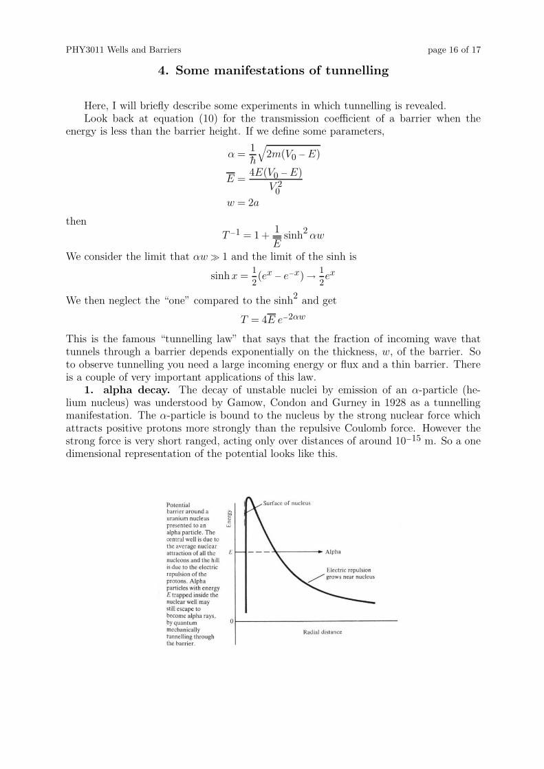
1. alpha decay. The decay of unstable nuclei by emission of an α-particle (he-lium nucleus) was understood by Gamow, Condon and Gurney in 1928 as a tunnellingmanifestation. The α-particle is bound to the nucleus by the strong nuclear force whichattracts positive protons more strongly than the repulsive Coulomb force. However thestrong force is very short ranged, acting only over distances of around 10−15 m. So a onedimensional representation of the potential looks like this.


The combination of the two potential energies (strong and Coulomb) amount to abarrier that the α-particle might tunnel through. The higher the energy of the particlethe greater the probability of emission (once it escapes the pull of the strong force it’simmediately repelled from the positive nucleus by the Coulomb force). In fact the tun-nelling law predicts that the logarithm of the lifetime is proportional to the inverse squareroot of the α-particle’s energy. This is confirmed for a large number of nuclei in the plotbelow.

2. The scanning tunnelling mi-

croscope was invented in 1981 by Bin-nig and Rohrer, who received the No-bel Prize in physics for their inventionin 1986. You probably know how itworks; here I just want to show a fig-ure from one of their papers showingthe logarithmic dependence of the tun-nelling current on the gap between thetip and the sample, as predicted by thetunnelling law.

1. The inﬁnite square well - Queen's University Belfast · 1. The inﬁnite square well ... even...

Documents

Transcript of 1. The inﬁnite square well - Queen's University Belfast · 1. The inﬁnite square well ... even...