1

Support Vector Machines Podpůrné vektorové stroje

Babak Mahdian,June 2009

2

Most of slides are taken from the presentations provided by:

1. Chih-Jen Lin (National Taiwan University)2. Colin Campbell (Bristol University)3. Andrew W. Moore (Carnegie Mellon University) 4. Jan Flusser (AS CR, ÚTIA)

3

Outline

1. SVMs for binary classification.

2. Soft margins and multi-class classification.

4

A classifier derived from statistical learning by Vladimir Vapnik et al. in 1992.

Currently SVM is widely used in object detection & recognition, content-based image retrieval, text recognition, biometrics, speech recognition, etc.

5

Preliminaries: Consider a binary classification problem: input vectors are xi and yi = {1,-1} are the targets or labels. The index i labels the pattern pairs (i = 1,…,m).

The xi define a space of labelled points called input space.

6

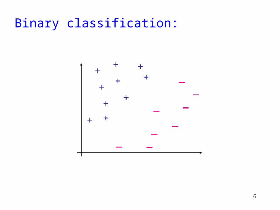
Binary classification:

7

Let us to separate the input data via a hyperplane.

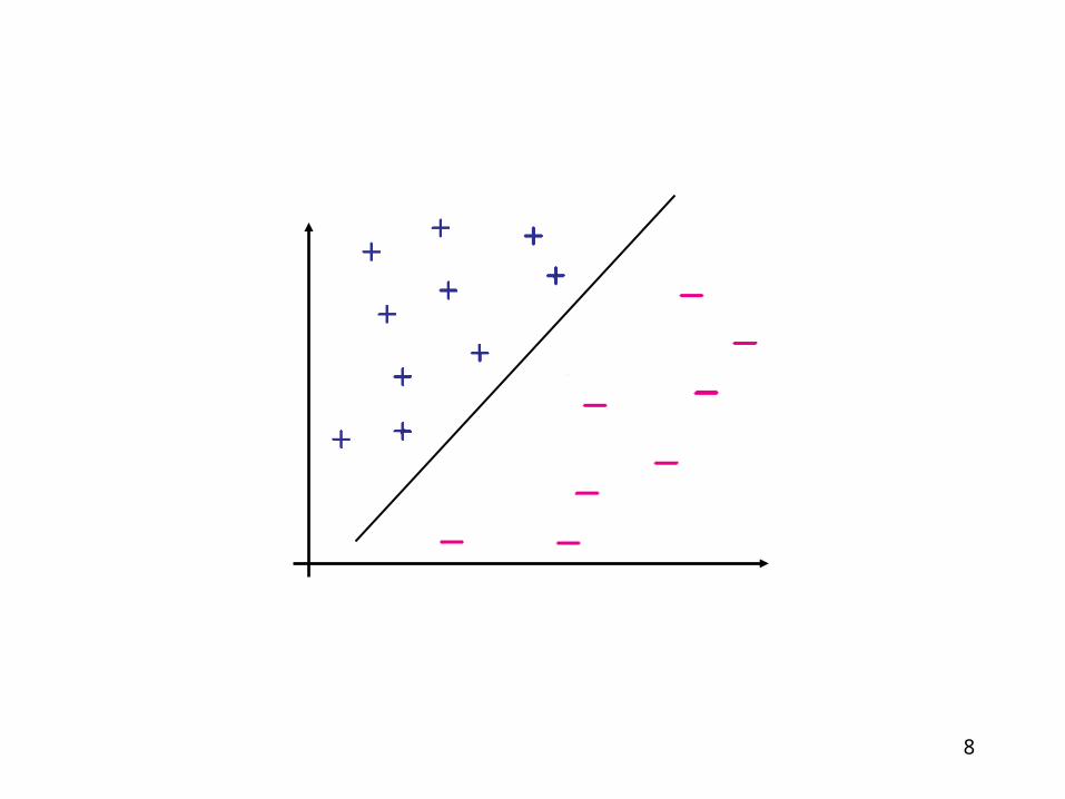
8

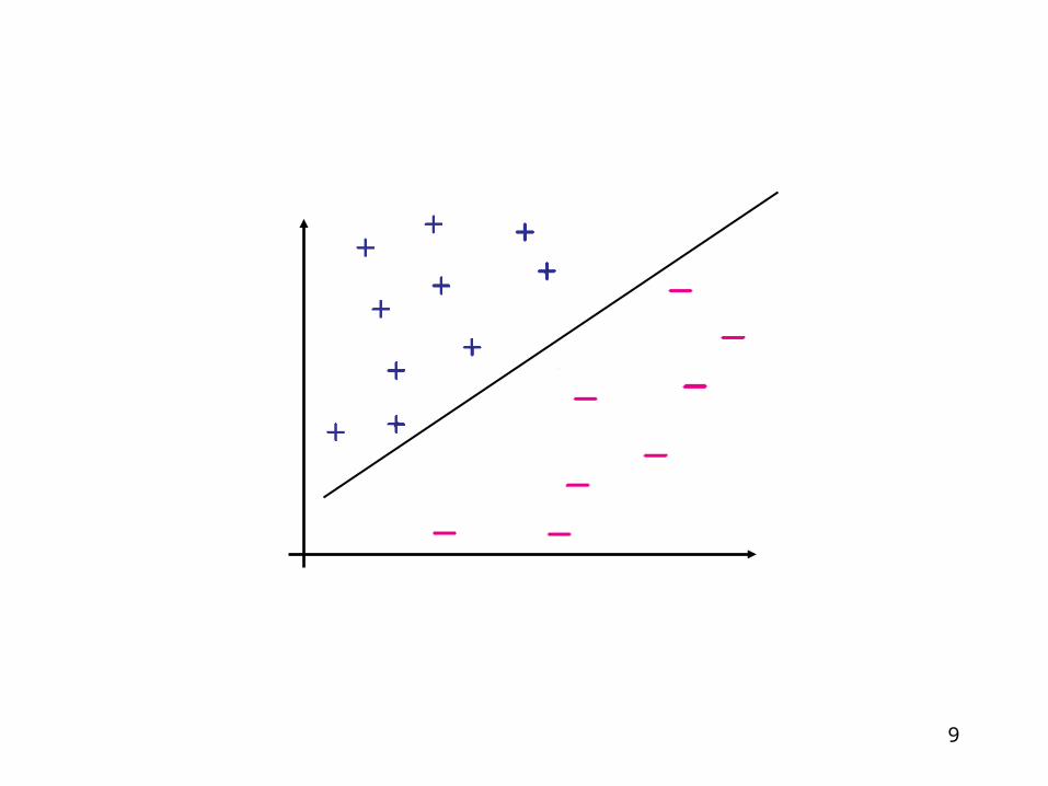
9

10

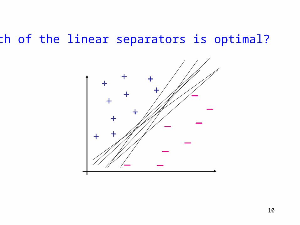
Which of the linear separators is optimal?

11

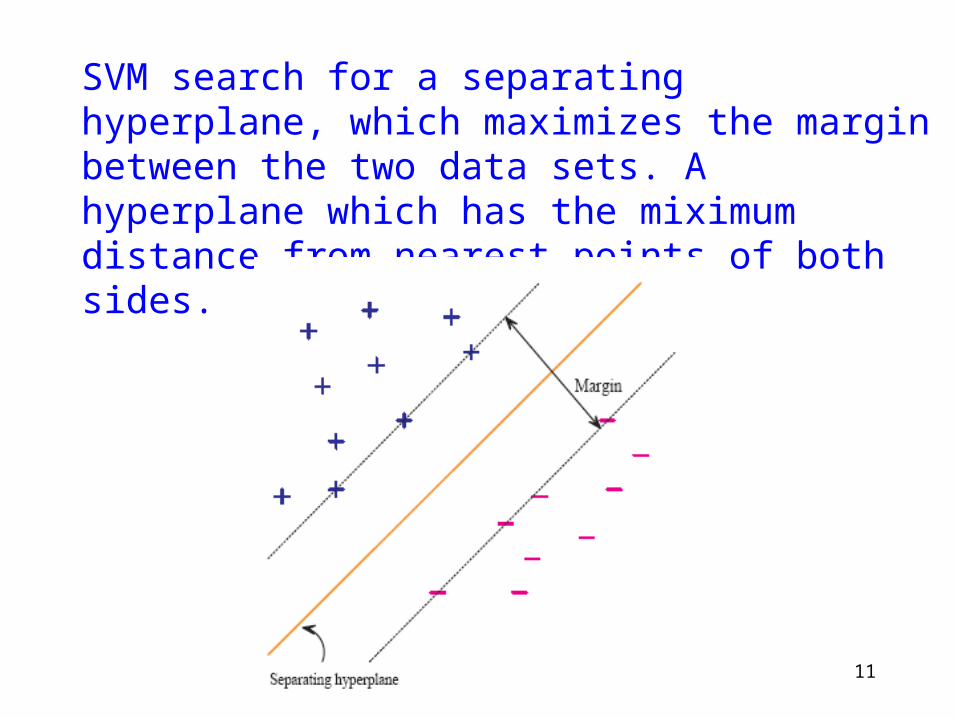
SVM search for a separating hyperplane, which maximizes the margin between the two data sets. A hyperplane which has the miximum distance from nearest points of both sides.

12

Such a hyperplane exhibits the best generalization.

It creates a “safe zone”.

The closest points are called support vectors (they directly support where the hyperplane should be).

Any change in support vectors shift the hyperplane.

Any change in non-support vectors do not shift the hyperplane.

13

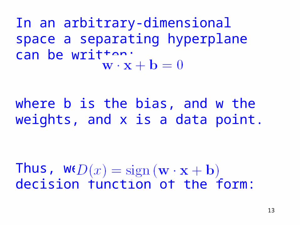
In an arbitrary-dimensional space a separating hyperplane can be written:

where b is the bias, and w the weights, and x is a data point.

Thus, we will consider a decision function of the form:

14

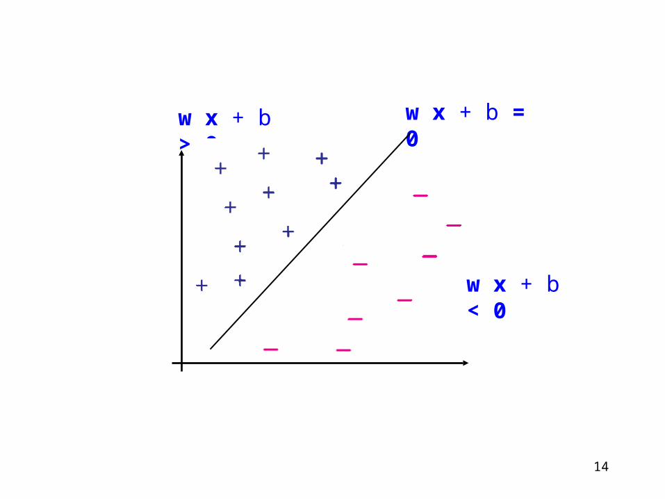
w x + b > 0

w x + b < 0

w x + b = 0

15

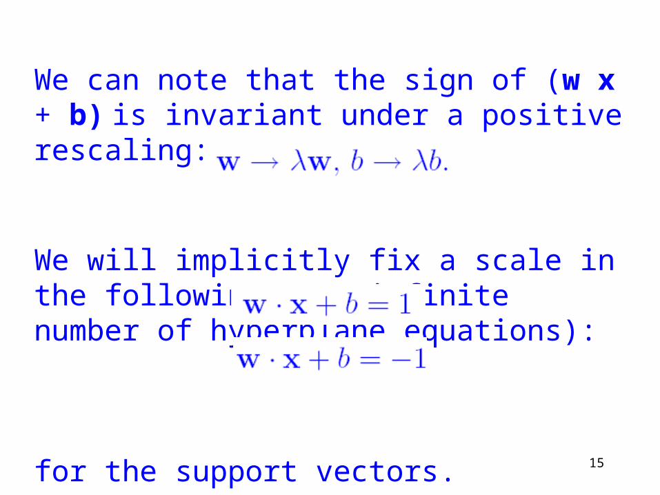
We can note that the sign of (w x + b) is invariant under a positive rescaling:

We will implicitly fix a scale in the following way (infinite number of hyperplane equations):

for the support vectors.

16

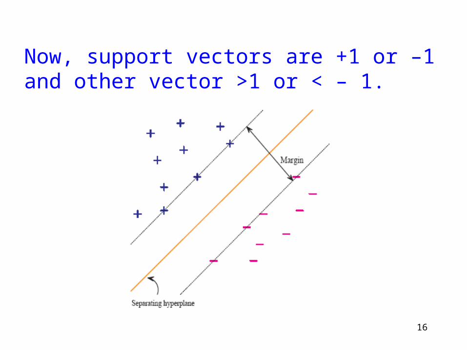
Now, support vectors are +1 or –1 and other vector >1 or < – 1.

17

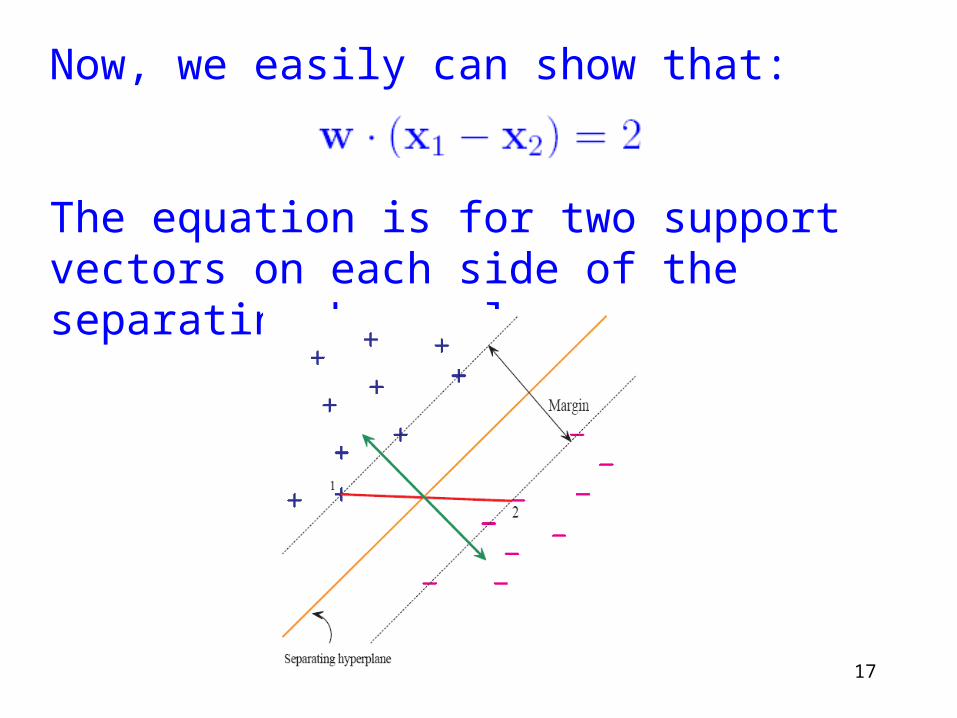
Now, we easily can show that:

The equation is for two support vectors on each side of the separating hyperplane.

18

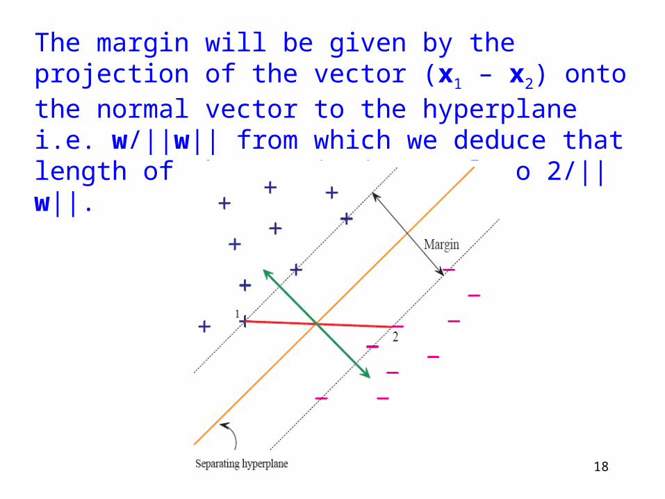
The margin will be given by the projection of the vector (x1 – x2) onto the normal vector to the hyperplane i.e. w/||w|| from which we deduce that length of the margin is equal to 2/||w||.

19

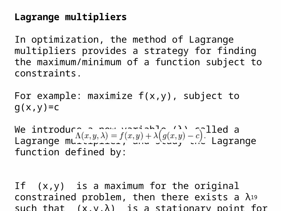
Lagrange multipliers

In optimization, the method of Lagrange multipliers provides a strategy for finding the maximum/minimum of a function subject to constraints.

For example: maximize f(x,y), subject to g(x,y)=c

We introduce a new variable (λ) called a Lagrange multiplier, and study the Lagrange function defined by:

If (x,y)  is a maximum for the original constrained problem, then there exists a λ such that (x,y,λ)  is a stationary point for the Lagrange function.

20

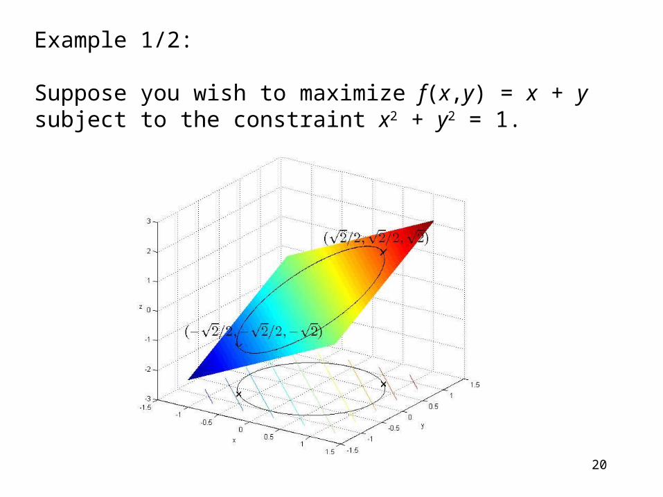
Example 1/2:

Suppose you wish to maximize f(x,y) = x + y subject to the constraint x2 + y2 = 1.

21

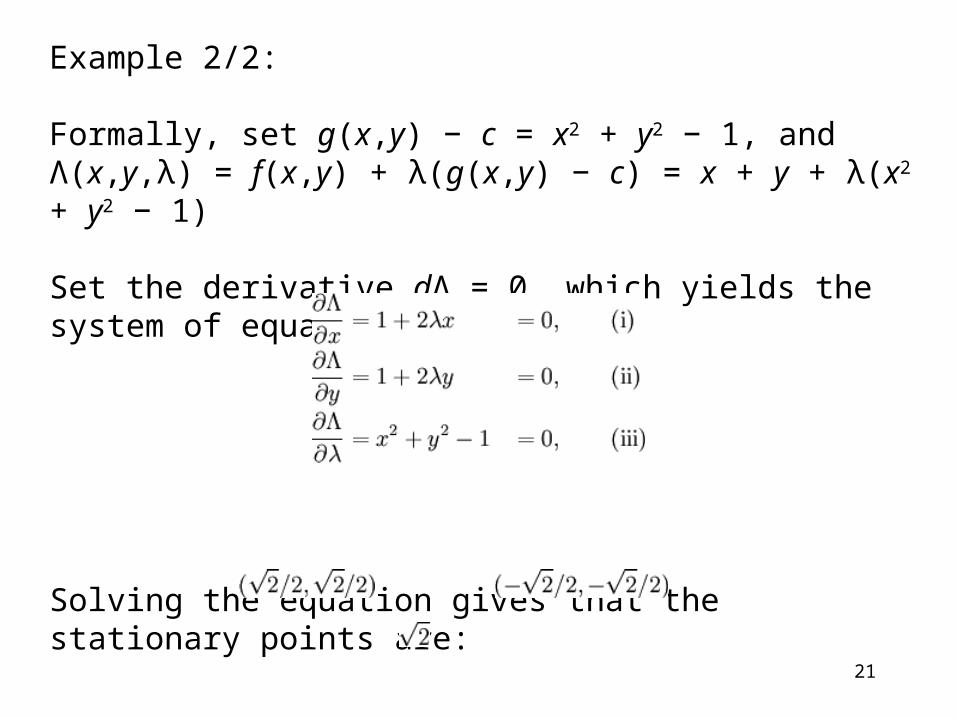
Example 2/2:

Formally, set g(x,y) − c = x2 + y2 − 1, and Λ(x,y,λ) = f(x,y) + λ(g(x,y) − c) = x + y + λ(x2 + y2 − 1)

Set the derivative dΛ = 0, which yields the system of equations:

Solving the equation gives that the stationary points are:

which gives the maximum

22

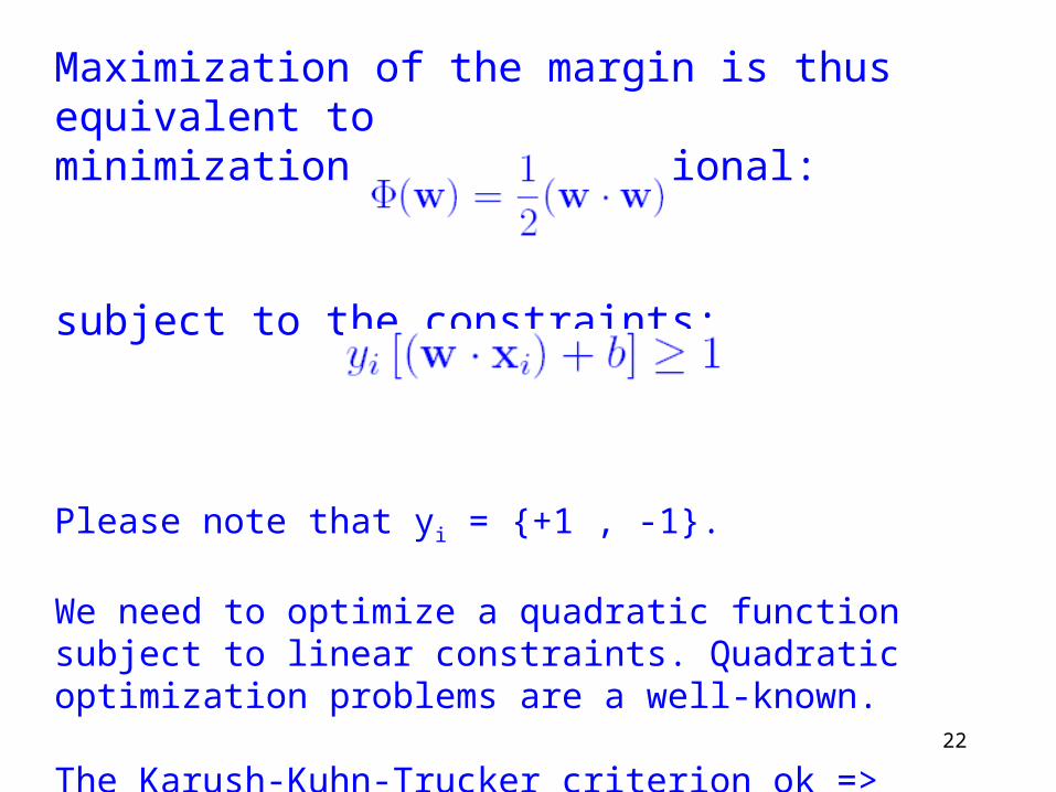
Maximization of the margin is thus equivalent tominimization of the functional:

subject to the constraints:

Please note that yi = {+1 , -1}.

We need to optimize a quadratic function subject to linear constraints. Quadratic optimization problems are a well-known.

The Karush-Kuhn-Trucker criterion ok => Lagrange

23

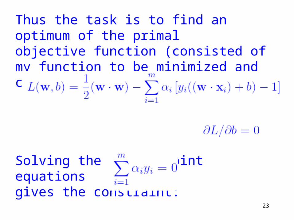
Thus the task is to find an optimum of the primalobjective function (consisted of my function to be minimized and constraints):

Solving the saddle point equationsgives the constraint:

24

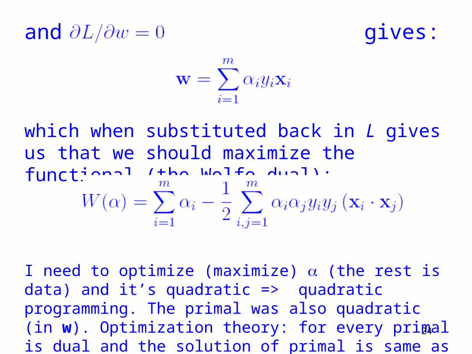
and gives:

which when substituted back in L gives us that we should maximize the functional (the Wolfe dual):

I need to optimize (maximize) (the rest is data) and it’s quadratic => quadratic programming. The primal was also quadratic (in w). Optimization theory: for every primal is dual and the solution of primal is same as the solution of dual.

25

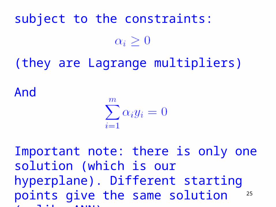
subject to the constraints:

(they are Lagrange multipliers)

And

Important note: there is only one solution (which is our hyperplane). Different starting points give the same solution (unlike ANN).

26

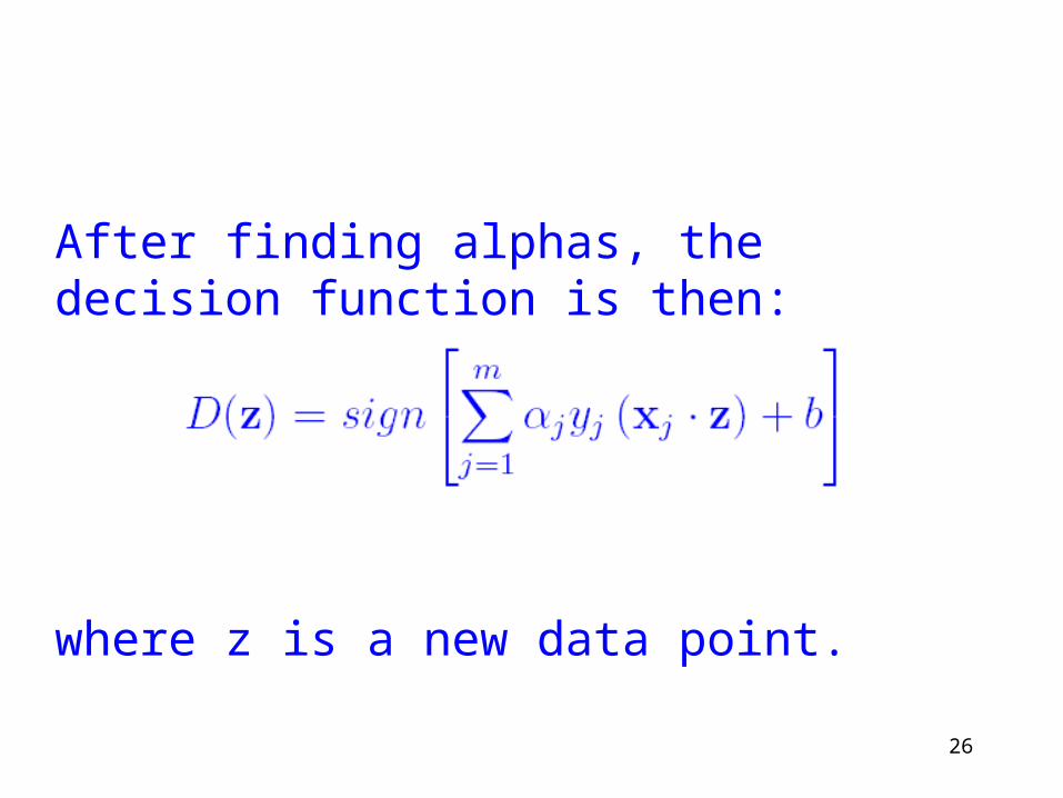
After finding alphas, the decision function is then:

where z is a new data point.

27

6=1.4

1=0.8

2=0

3=0

4=0

5=07=0

8=0.6

9=0

10=0

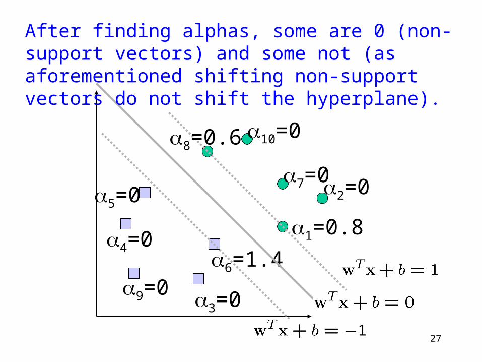
After finding alphas, some are 0 (non-support vectors) and some not (as aforementioned shifting non-support vectors do not shift the hyperplane).

28

Some alphas are zero, some non-zero and sometime some are very large.

Two reasons: 1. a correct, but unusual data point 2. an outlier

Very large alphas have a big influence on hyperplane’s position.

29

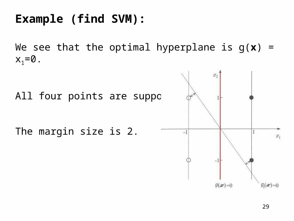
Example (find SVM):

We see that the optimal hyperplane is g(x) = x1=0.

All four points are support vectors.

The margin size is 2.

30

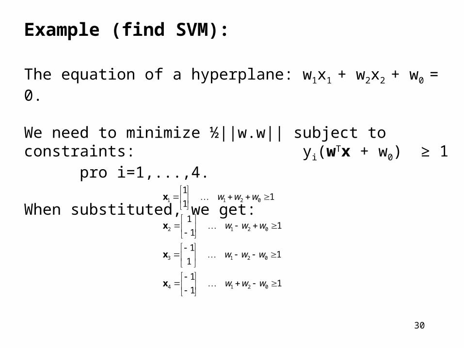
Example (find SVM):

The equation of a hyperplane: w1x1 + w2x2 + w0 = 0.

We need to minimize ½||w.w|| subject to constraints: yi(wTx + w0) ≥ 1 pro i=1,...,4.

When substituted, we get:

11

1

11

1

11

1

11

1

0214

0213

0212

0211

www

www

www

www

x

x

x

x

31

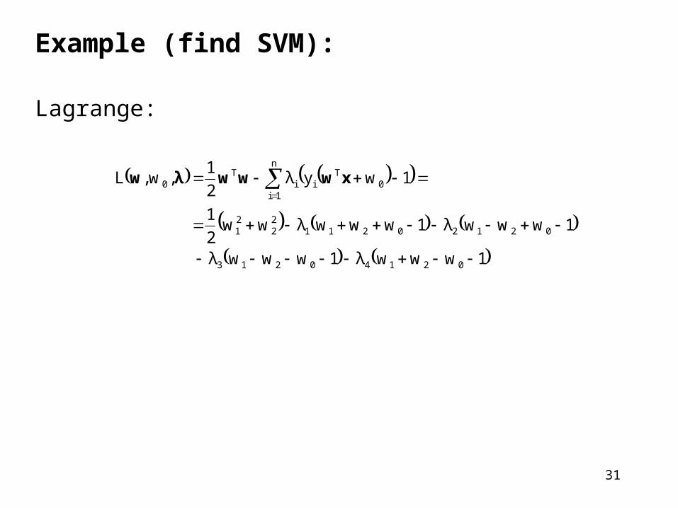
Example (find SVM):

Lagrange:

1wwwλ1wwwλ

1wwwλ1wwwλww2

1

1wyλ2

1,w,L

02140213

0212021122

21

n

1i0

Tii

T0

xwwwλw

32

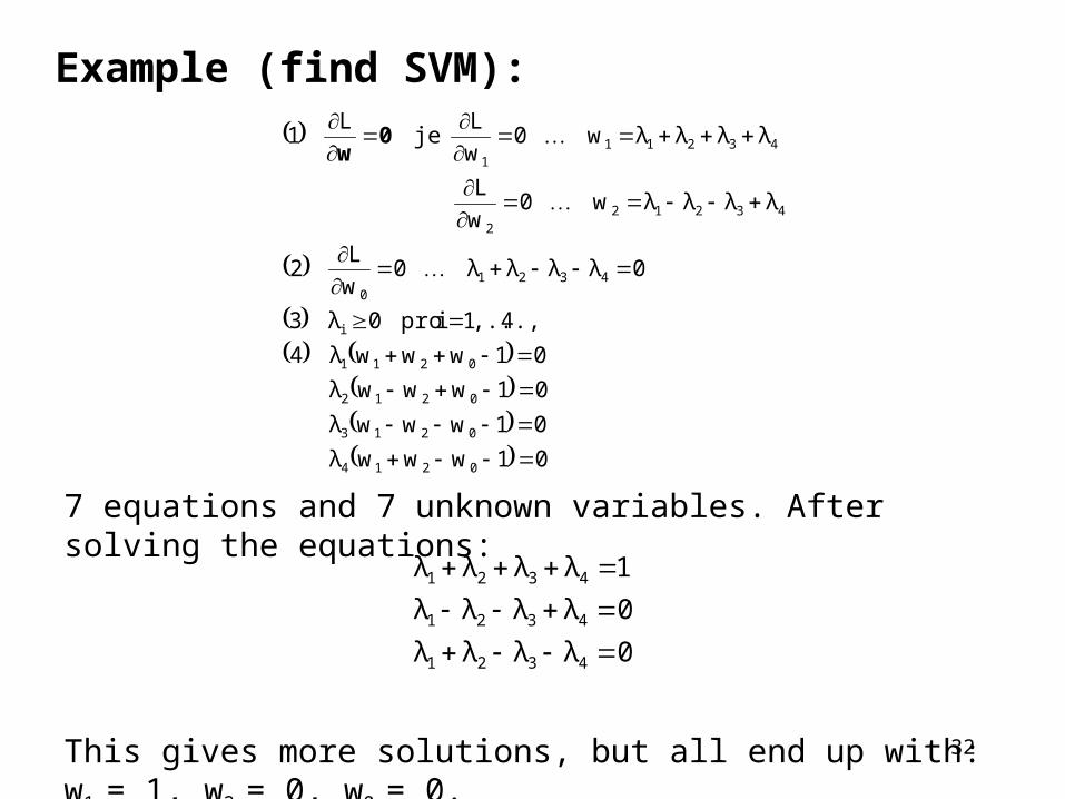
Example (find SVM):

01wwwλ

01wwwλ

01wwwλ

01wwwλ4

4,...,1ipro0λ3

0λλλλ0w

L2

λλλλw0w

L

λλλλw0w

Lje

L1

0214

0213

0212

0211

i

43210

432122

432111

0w

7 equations and 7 unknown variables. After solving the equations:

This gives more solutions, but all end up with: w1 = 1, w2 = 0, w0 = 0.

0λλλλ

0λλλλ

1λλλλ

4321

4321

4321

33

Recap:

1. The classifier is a separating hyperplane.

2. Most “important” training points are support vectors; they define the hyperplane.

3. Quadratic optimization algorithms can identify which training points xi are support vectors with non-zero Lagrangian multipliers αi .

34

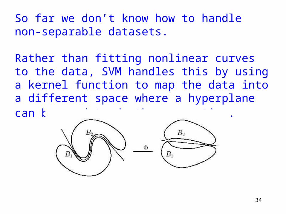
So far we don’t know how to handle non-separable datasets.

Rather than fitting nonlinear curves to the data, SVM handles this by using a kernel function to map the data into a different space where a hyperplane can be used to do the separation.

35

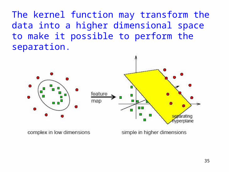
The kernel function may transform the data into a higher dimensional space to make it possible to perform the separation.

36

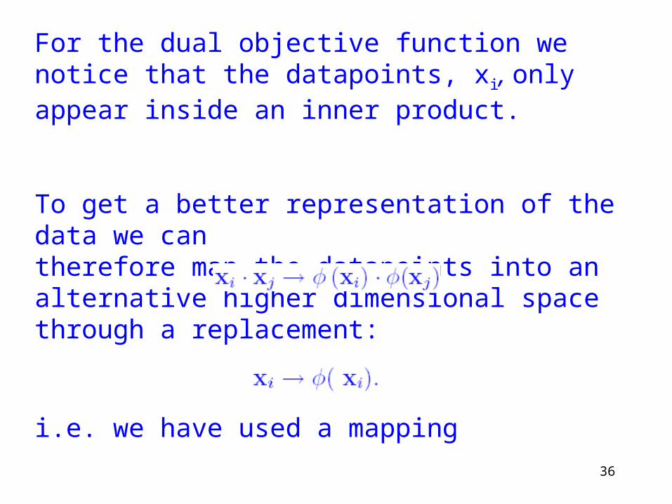
For the dual objective function we notice that the datapoints, xi, only appear inside an inner product.

To get a better representation of the data we cantherefore map the datapoints into an alternative higher dimensional space through a replacement:

i.e. we have used a mapping

This higher dimensional space must be a Hilbert Space.

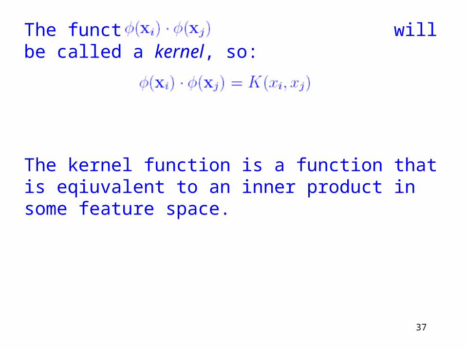
37

The function will be called a kernel, so:

The kernel function is a function that is eqiuvalent to an inner product in some feature space.

38

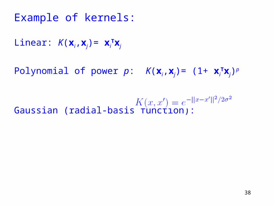
Example of kernels:

Linear: K(xi,xj)= xiTxj

Polynomial of power p: K(xi,xj)= (1+ xiTxj)p

Gaussian (radial-basis function):

39

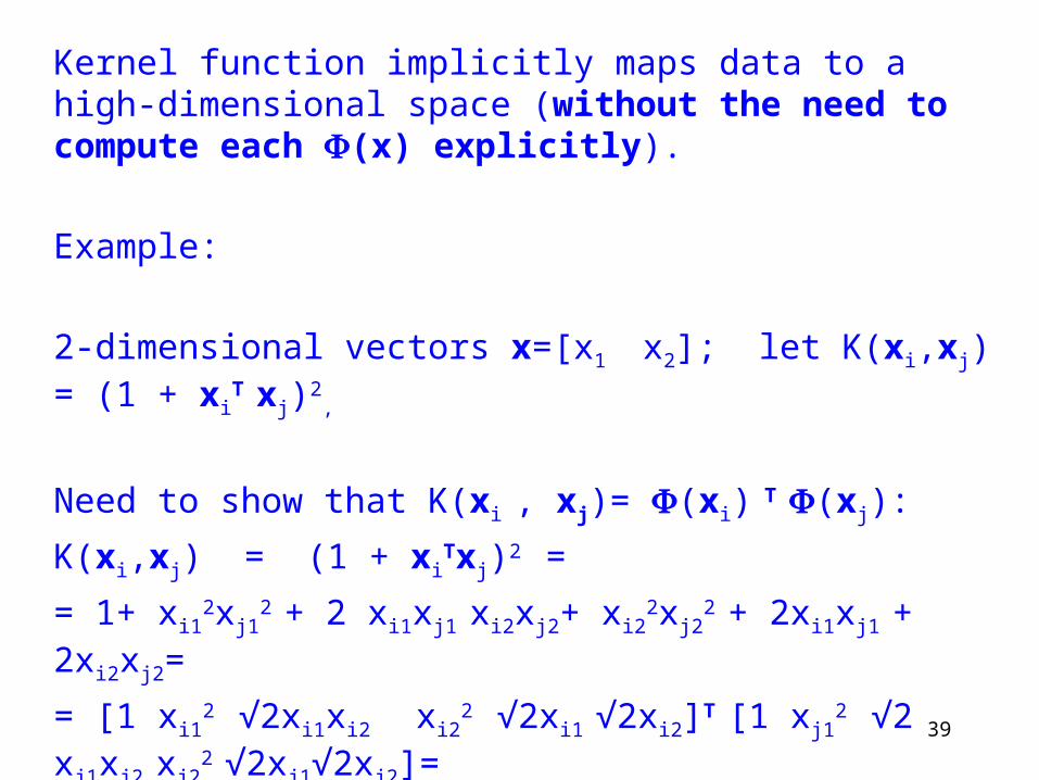
Kernel function implicitly maps data to a high-dimensional space (without the need to compute each (x) explicitly).

Example:

2-dimensional vectors x=[x1 x2]; let K(xi,xj) = (1 + xi

T xj)2,

Need to show that K(xi , xj)= (xi) T (xj):

K(xi,xj) = (1 + xiTxj)2 =

= 1+ xi12xj1

2 + 2 xi1xj1 xi2xj2+ xi2

2xj22 + 2xi1xj1 + 2xi2xj2=

= [1 xi12 √2xi1xi2 xi2

2 √2xi1 √2xi2]T [1 xj12 √2 xj1xj2 xj2

2

√2xj1√2xj2]=

= (xi) (xj),

where (x) = [1 x12 √2 x1x2 x2

2 √2x1 √2x2]

40

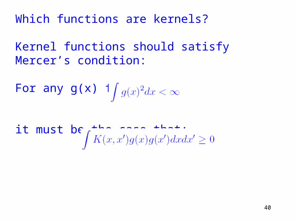
Which functions are kernels?

Kernel functions should satisfy Mercer’s condition:

For any g(x) for which:

it must be the case that:

41

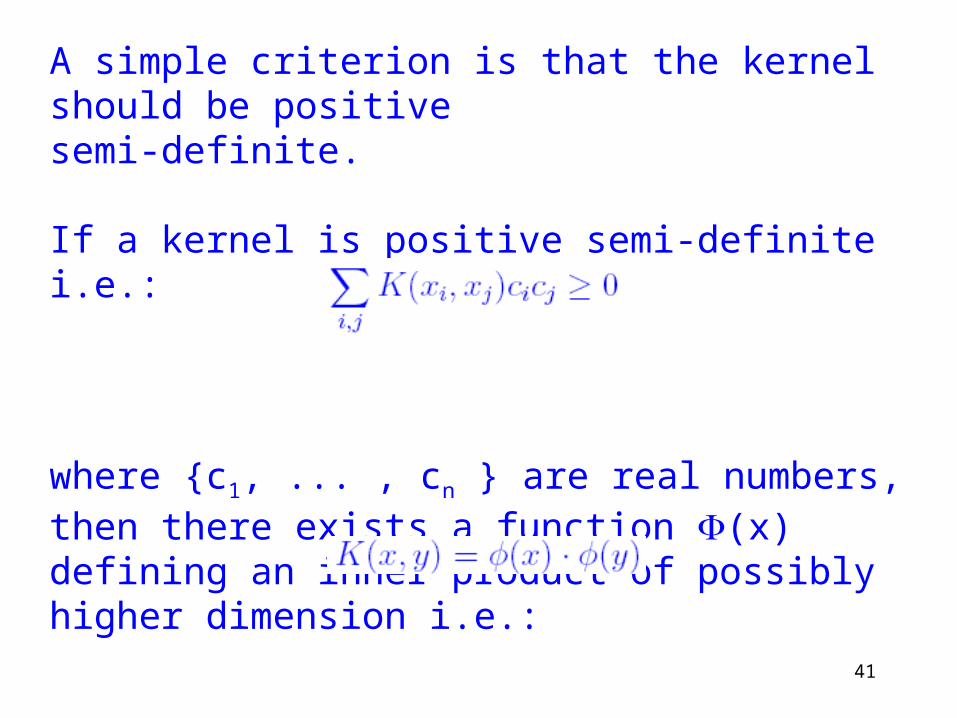
A simple criterion is that the kernel should be positivesemi-definite.

If a kernel is positive semi-definite i.e.:

where {c1, ... , cn } are real numbers, then there exists a function (x) defining an inner product of possibly higher dimension i.e.:

42

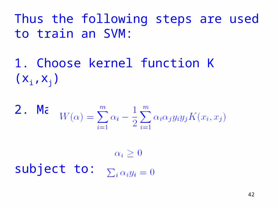
Thus the following steps are used to train an SVM:

1. Choose kernel function K (xi,xj)

2. Maximize:

subject to:

43

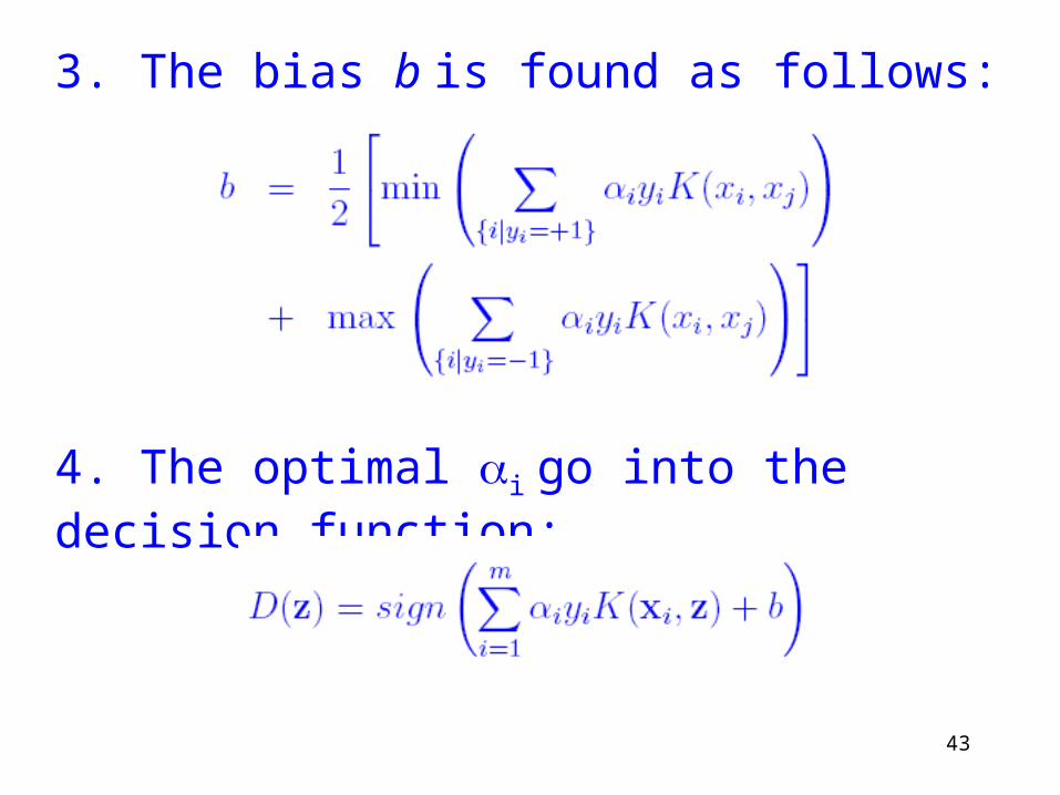
3. The bias b is found as follows:

4. The optimal i go into the decision function:

44

Choosing the Kernel Function and its parameters

Probably the most tricky part of using SVM.

Many principles have been proposed.

In practice, a low degree polynomial kernel or RBF kernel with a reasonable width is a good initial try for most applications.

It was said that for text classification, linear kernel is the best choice, because of the high feature dimension.

45

Multi-class problems

SVM constructed for binary classification.

Multi-class classification: Many problems involvemulticlass classification.

A number of schemes have been outlined.

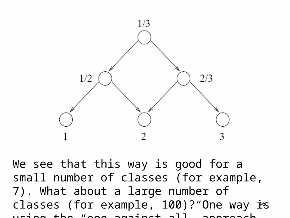
One of the simplest schemes is to use a directed acyclic graph (DAG) with the learning task reduced to binary classification at each node:

46

We see that this way is good for a small number of classes (for example, 7). What about a large number of classes (for example, 100)? One way is using the “one against all” approach.

47

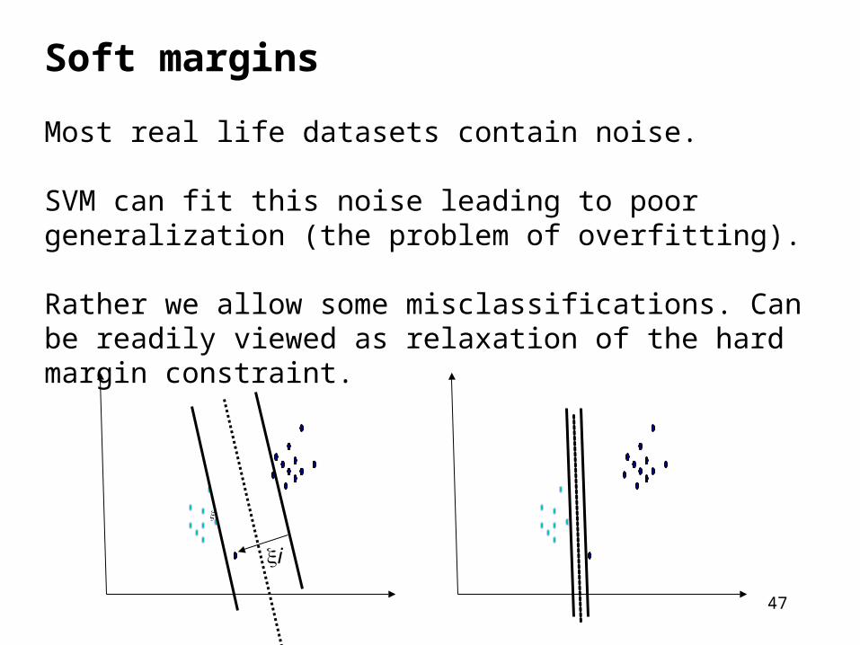
Soft margins

Most real life datasets contain noise.

SVM can fit this noise leading to poor generalization (the problem of overfitting).

Rather we allow some misclassifications. Can be readily viewed as relaxation of the hard margin constraint.

i

i

48

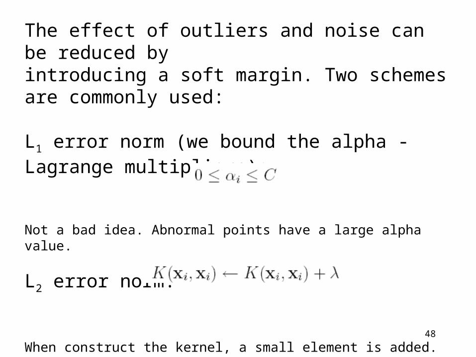
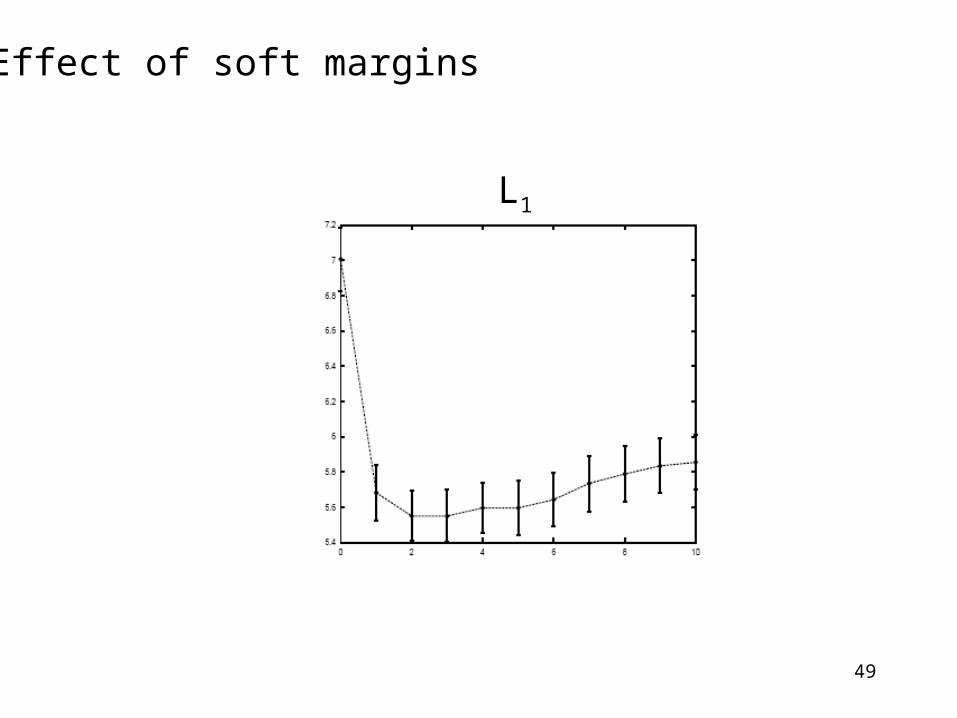
The effect of outliers and noise can be reduced byintroducing a soft margin. Two schemes are commonly used:

L1 error norm (we bound the alpha - Lagrange multipliers):

Not a bad idea. Abnormal points have a large alpha value.

L2 error norm:

When construct the kernel, a small element is added.

49

Effect of soft margins

L1

50

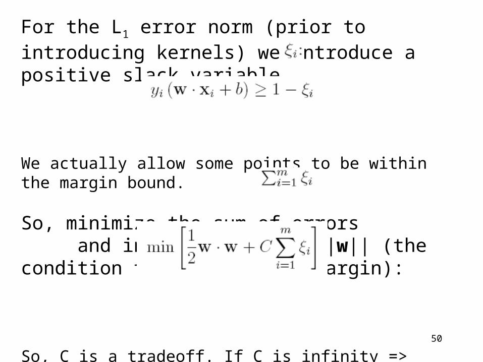
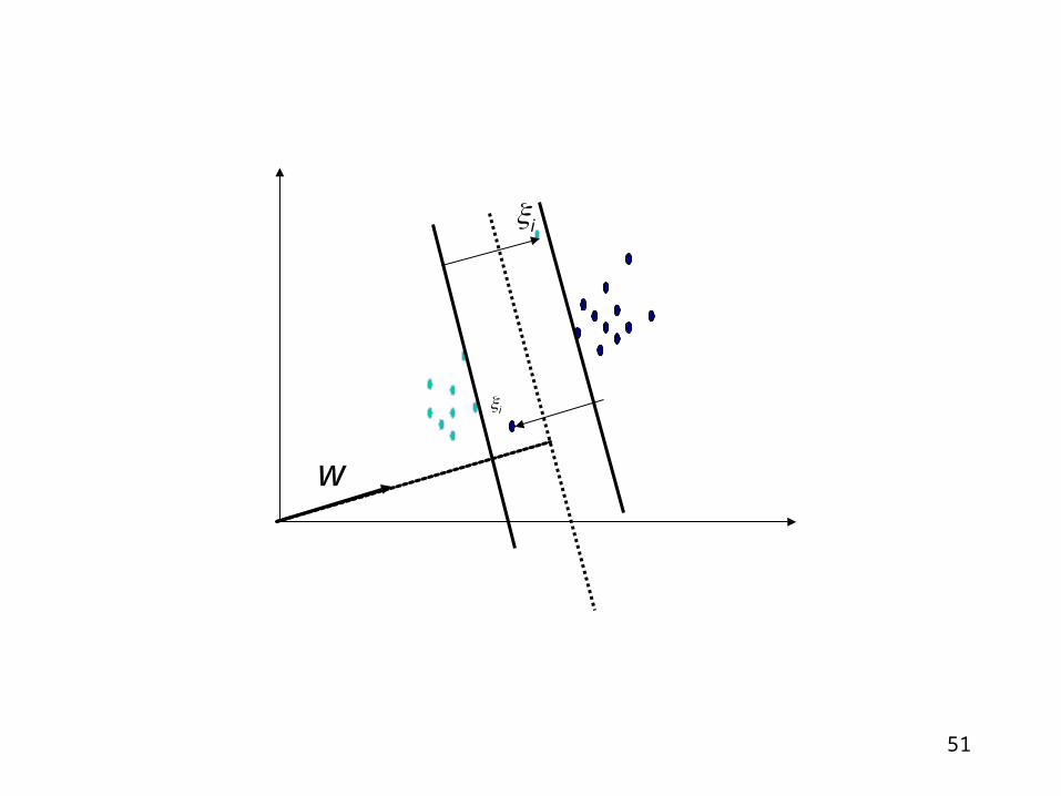
For the L1 error norm (prior to introducing kernels) we introduce a positive slack variable

We actually allow some points to be within the margin bound.

So, minimize the sum of errors and in the same time ||w|| (the condition to maximize the margin):

So, C is a tradeoff. If C is infinity => normal hard margin. If C < infinity, we will have some terms being non-zero among the slack variables.

51

i

w

i

52

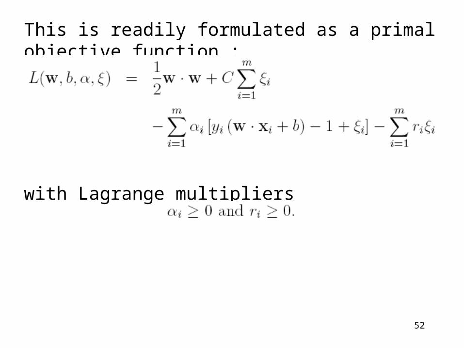
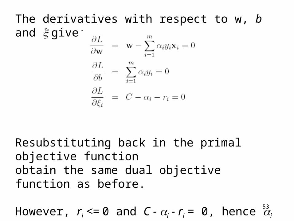
This is readily formulated as a primal objective function :

with Lagrange multipliers

53

The derivatives with respect to w, b and give:

Resubstituting back in the primal objective functionobtain the same dual objective function as before.

However, ri <= 0 and C - i - ri = 0, hence i <= C andthe constraint 0 <= i is replaced by 0 <= i <= C.

54

Patterns with values 0 <= i <= C will be referred to as non-bound and those with i = 0 or i = C will be said to be at bound.

Some theory about the optimal value C.

In practice, the optimal value of C must be found by experimentation using a validation.

55

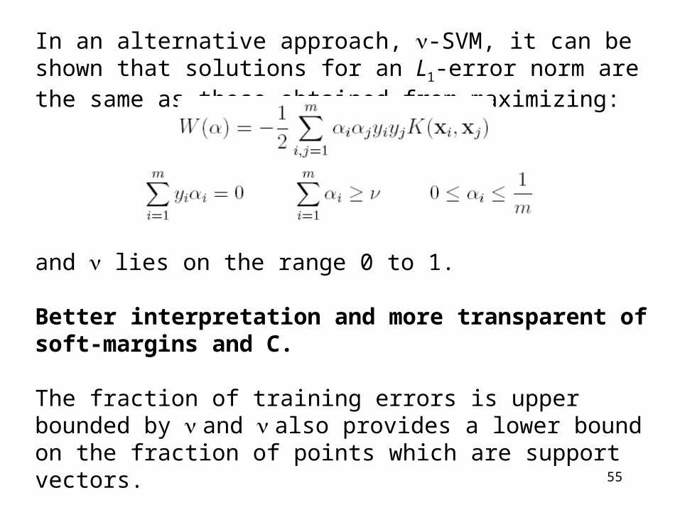
In an alternative approach, -SVM, it can be shown that solutions for an L1-error norm are the same as those obtained from maximizing:

and lies on the range 0 to 1.

Better interpretation and more transparent of soft-margins and C.

The fraction of training errors is upper bounded by and also provides a lower bound on the fraction of points which are support vectors.

56

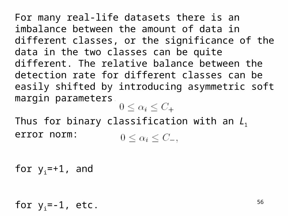
For many real-life datasets there is an imbalance between the amount of data in different classes, or the significance of the data in the two classes can be quite different. The relative balance between the detection rate for different classes can be easily shifted by introducing asymmetric soft margin parameters.

Thus for binary classification with an L1 error norm:

for yi=+1, and

for yi=-1, etc.

Thus, it allows a control on false positives rate. We do a favor for one class.

57

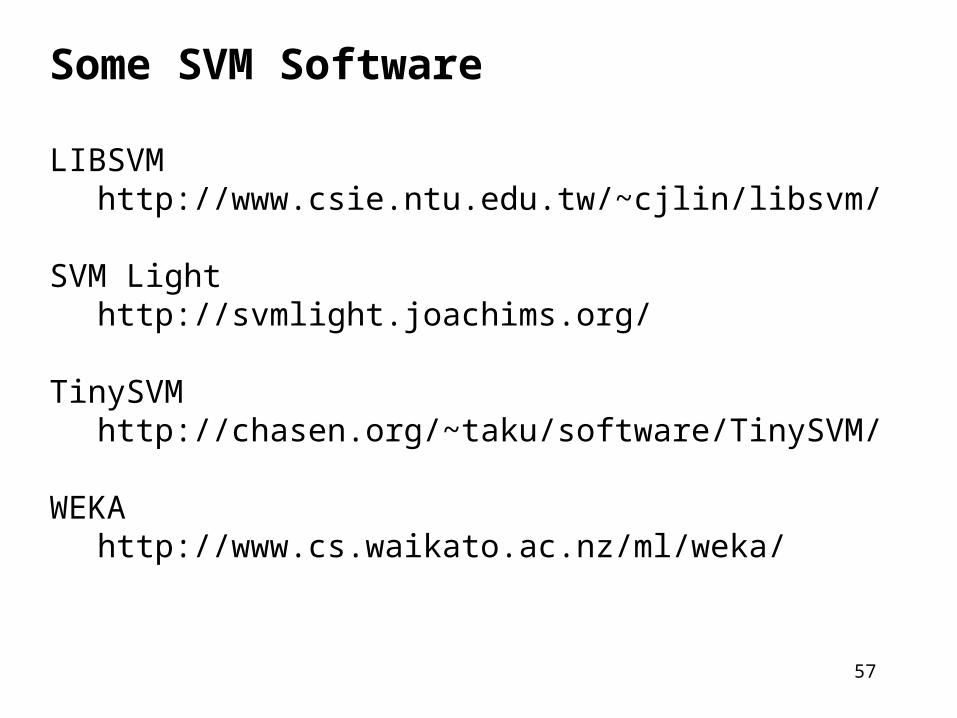
Some SVM Software

LIBSVMhttp://www.csie.ntu.edu.tw/~cjlin/libsvm/

SVM Lighthttp://svmlight.joachims.org/

TinySVMhttp://chasen.org/~taku/software/TinySVM/

WEKAhttp://www.cs.waikato.ac.nz/ml/weka/

58

Conclusion

SVMs are currently among the better performers for a number of classification tasks.

SVM techniques have been extended to a number of tasks such as regression.

Tuning SVMs remains a black art: selecting a specific kernel and parameters is usually done in a try-and-see manner (a lengthy series of experiments in which various parameters are tested).