1 Structural importance - Santa Fe...

Network Analysis and Modeling, CSCI 5352Lecture 2

Prof. Aaron Clauset2017

1 Structural importance

A common question we may ask when analyzing the structure of a network is

Which vertices are important?

How we answer this question depends on what exactly we mean by important, and there are severalgeneral approaches to answering it. The two most common are structural importance and dynam-ical importance. Every approach defines an importance function f : G→ ~v, which takes as input agraph G and returns a vector ~v containing the ranks or importance scores of its vertices V . Hence,this is an unsupervised learning setting, where we choose an f and see what comes out. (Supervisedlearning (to rank) in this kind of setting is active area of research)

Dynamical importance defines a node as important based on some kind of dynamical process run-ning on top of the network structure. For instance, a vertex u could be important if changes tou’s state variable xu produce changes to the variables attached to many other vertices (a behaviorone might be tempted to call “influence”),1 as in the case of spreading diseases or memes. As aresult, dynamical importance defines importance jointly, in terms of both structure and dynamics.Measures of dynamical importance can thus be expensive to compute, especially if they requiredirect simulation.

In contrast, structural importance means defining a node’s importance only in terms the network’sstructure, e.g., being the most or “best” connected vertex or being in the “middle” of the network.Depending on the particular measures we choose, a structurally important vertex may not also bedynamically important, and vice versa. When the two are correlated (which is often the case!),we can sometimes avoid an expensive computation of dynamical importance by computing thecorrelated structural importance instead. But, be careful: it is common to assume that dynami-cal (or even functional) importance is equivalent to structural importance, but this may not be true.

In this lecture, we will study measures of structural importance, which serve as the foundation ofthe more complicated measures of dynamical or functional importance. Structural importance mea-sures are also very useful for developing network intuition. Understanding how different measuresproduce different results on the same network will illustrate key network concepts and measures.

Measures of structural importance are often called centrality measures—a term from sociology—and we say that more central vertices are more structurally important while less central ones are

1The term “influence” is like the term “importance” in that it is not well defined. An unfortunate fact of theliterature on network influence is that there is no accepted rigorous definition of influence, no rigorous accepted wayto measure it, and thus little rigorous science. There are some good papers on influence in networks, but they arefew and far between.

1



less structurally important.2 A key caveat about importance measures is that every such measuremakes assumptions about what importance means. In applied settings, it is thus crucial to considerwhether or not those assumptions fit with the system or question of interest. Because centralitymeasures are simply functions of the adjacency matrix, they can always be calculated. However,the value of such a calculation may not be large.

As a running example for these centrality measures, we will apply each to a single network: thepopular Zachary’s karate club network,3 which represents the social network of friendships between34 members of a karate club at a US university in the 1970s. During the course of Zachary’s study,the club split into two factions, centered around two leaders in the club (nodes 1 and 34). Thispicture shows the network and the final partition.

1

2

3

4

5

6

7

8

9

10

11

12

13

14

15

16

17

18

19

20

21

22

23

24

25 26

27

28

29

30

31

32

33

34

2 Degree centrality

The simplest measure of importance is the degree of a vertex ki, i.e., the number of edges thatterminate or originate at i.4 The idea is that vertices with larger degrees exert greater effect onthe network, and thus identifying the most connected vertices is a useful way to identify theseimportant vertices. In many situations, these highly-connected vertices play special roles in bothlarge-scale organization of the network and in the dynamics of network processes. We will returnto these ideas later in greater detail.

2Under a specific model of dynamics, structural and dynamical importance can be equivalent. Changing themodel changes the way one calculates the structural importance measure. For a good discussion of the subtleties, seeS. P. Borgatti, “Centrality and network flow.” Social Networks 27, 55–71 (2005).

3W. W. Zachary, “An information flow model for conflict and fission in small groups.” J. Anthropol. Res. 33,452–473 (1977).

4The degree of a vertex k is sometimes called degree centrality in sociology.

2



This figure shows the karate club network in which the area of each vertex’s circle is proportionalto its degree in the network, and the table lists the degree k and normalized degree k/m for eachvertex.

1

2

3

4

5

6

7

8

9

10

11

13

14

15

16

17

18

19

20

21

22

23

24

25 26

27

28

29

30

31

32

33

34

12

group 1 1 2 3 4 5 6 7 8 11 12 13 14 17 18 20 22k 16 9 10 6 3 4 4 4 3 1 2 5 2 2 3 2

k/m 0.10 0.06 0.06 0.04 0.02 0.03 0.03 0.03 0.02 0.01 0.01 0.03 0.01 0.01 0.02 0.01

group 2 9 10 15 16 19 21 23 24 25 26 27 28 29 30 31 32 33 34k 5 2 2 2 2 2 2 5 3 3 2 4 3 4 4 6 12 17

k/m 0.03 0.01 0.01 0.01 0.01 0.01 0.01 0.03 0.02 0.02 0.01 0.03 0.02 0.03 0.03 0.04 0.08 0.11

2.1 Centrality from eigenvectors

The degree of a vertex captures only a local measure of importance, and a natural generalization ofdegree centrality is to increase the importance of vertices who are connected to other high-degreevertices. That is, not all neighbors are equal and perhaps a node’s importance should be larger ifit is connected to other important vertices. Eigenvector centrality accounts for these differences byassigning a vertex an importance score that is proportional to the importance scores of its neighbors.

There are several ways to formalize this recursive notion of importance, and each approach producesslightly different final scores. However, they are all forms of eigenvector centrality because they canbe calculated as the principal eigenvector5 for a particular eigenvalue problem—the differences layin how we set up that problem. Here we will cover eigenvector centrality (as defined by Bonacich)and PageRank. Other popular versions are the Katz centrality and hub/authority scores, which wewill not cover here.

5The eigenvector associated with the largest (most positive) eigenvalue.

3



Eigenvector centralityTaking the recursive idea about importance at face value, we may write down the following equation:

x(t+1)i =

n∑j=1

Aijx(t)j , (1)

where Aij is an element of the adjacency matrix (and thus selects contributions to i’s importance

based on whether i and j are connected), and with the initial condition x(0)i = 1 for all i.

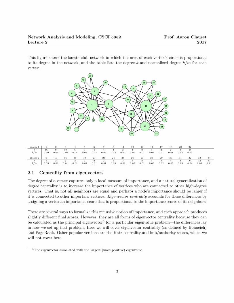
This formulation is a model in which each vertex “votes” for the importance of its neighbors bytransferring some of its importance to them. By iterating the equation, with the iteration numberindexed by t, importance flows across the network. However, this equation by itself will not pro-duce useful importance estimates because the values xi increase with t. But, absolute values arenot of interest themselves, and relative values may be derived by normalizing at any (or every) step.6

Applying this method to the karate club for different choices of t yields the following table. Noticethat by the t = 15th iteration, the vector x has essentially stopped changing, indicating conver-gence on a fixed point. (Convergence here is particularly fast in part because the network has asmall diameter.) Illustrating the close relationship between degree and eigenvector centrality, thecentrality scores here are larger among the high-degree vertices, e.g., 1, 34, 33, 3 and 2.

vertex x(1) x(5) x(10) x(15) x(20) degree, k1 0.103 0.076 0.071 0.071 0.071 162 0.058 0.055 0.053 0.053 0.053 93 0.064 0.065 0.064 0.064 0.064 104 0.038 0.043 0.042 0.042 0.042 65 0.019 0.015 0.015 0.015 0.015 36 0.026 0.016 0.016 0.016 0.016 47 0.026 0.016 0.016 0.016 0.016 48 0.026 0.034 0.034 0.034 0.034 49 0.032 0.044 0.046 0.046 0.046 510 0.013 0.020 0.021 0.021 0.021 211 0.019 0.015 0.015 0.015 0.015 312 0.006 0.010 0.011 0.011 0.011 113 0.013 0.017 0.017 0.017 0.017 214 0.032 0.044 0.046 0.045 0.045 515 0.013 0.019 0.021 0.020 0.020 216 0.013 0.019 0.021 0.020 0.020 217 0.013 0.005 0.005 0.005 0.005 218 0.013 0.018 0.019 0.019 0.019 219 0.013 0.019 0.021 0.020 0.020 220 0.019 0.028 0.030 0.030 0.030 321 0.013 0.019 0.021 0.020 0.020 222 0.013 0.018 0.019 0.019 0.019 223 0.013 0.019 0.021 0.020 0.020 224 0.032 0.029 0.030 0.030 0.030 525 0.019 0.012 0.011 0.011 0.011 326 0.019 0.013 0.012 0.012 0.012 327 0.013 0.015 0.015 0.015 0.015 228 0.026 0.026 0.027 0.027 0.027 429 0.019 0.026 0.026 0.026 0.026 330 0.026 0.026 0.027 0.027 0.027 431 0.026 0.034 0.035 0.035 0.035 432 0.038 0.037 0.039 0.038 0.038 633 0.077 0.066 0.062 0.062 0.062 1234 0.109 0.082 0.074 0.075 0.075 17

6Large values of t will tend to produce overflow errors in most matrix computations, and thus normalizing is anecessary component of a complete calculation.

4



The Perron-Frobenius theorem from linear algebra guarantees that when the network is an undi-rected, connected component, iterating Eq. (1) will always converge on a fixed point equivalent tothe principal eigenvector of the adjacency matrix.7 Thus, we can sidestep the iteration completelyand formulate the calculation as an eigenvector problem of the form

Ax = λ1x , (2)

where A is the adjacency matrix, x is a vector containing the eigenvector centralities, and λ1is the largest eigenvalue of A.8 Computing eigenvector centralities can be done in most modernmathematical computing software, or using common linear algebra libraries via matrix inversiontechniques (which take O(n3) time, but can be as fast as n2.373 or even n2 lnn depending on sometechnical details.). Doing so with the karate club network yields exactly the same values we foundabove, via the iterative approach.

To more clearly illustrate the relationship between eigenvector centrality and degree, we can com-pare the scores given to vertices under each. This figure shows the very strong correlation between

0 0.02 0.04 0.06 0.08 0.1 0.120

0.01

0.02

0.03

0.04

0.05

0.06

0.07

0.08

341

333

2

normalized degree, k/m

eig

en

ve

cto

r ce

ntr

alit

y,

x

eigenvector centrality and (normalized) degree centrality in the karate club. In fact, the Pearsoncorrelation coefficient between x and k/m is r2 = 0.84, indicating that knowing the value of one

7The Perron-Frobenius theorem provides the conditions under which this formulation holds: a real and irreduciblesquare matrix with non-negative entries will have a unique largest real eigenvalue and that the corresponding eigen-vector has non-negative components. What we are doing by iterating Eq. (1) is the “matrix power method” ofcomputing the principal eigenvector.

8Originally given in P. Bonacich, J. Math. Soc. 2, 113 (1972), and P. Bonacich, Social Meth. 4, 176 (1972).

5



provides a great deal of information about the value of the other. There are, of course, differences,as the scatter plot shows, and these are related to the way eigenvector centrality allows a vertex’simportance to be partly a function of the importance of its neighbors (and its neighbors’ neighbors),which is information not included in the degree of a vertex.

PageRankPageRank is another kind of eigenvector centrality,9 but which has some nicer features than theBonacich (and Katz) definitions. In particular, the classic eigenvector centrality performs poorlywhen applied to directed networks. In general, centralities will be zero for all vertices not within astrongly connected component, even if those vertices have high in-degree. Moreover, in an directedacyclic graph, there are no strongly connected components larger than a single vertex, and thusonly vertices with no out-going edges (kout = 0) will have non-zero centrality. These are not desir-able behaviors for a centrality score.

PageRank solves these problems by adding two features to our vertex voting model. First, it assignsevery vertex a small amount of centrality regardless of its network position. This eliminates theproblems caused by vertices with zero in-degree—who have no other way of gaining any centrality—and allows them to contribute to the centrality of vertices they link to. As a result, vertices withhigh in-degree will tend to have higher centrality as a result of being linked to, regardless of whetherthose neighbors themselves have any links to them. Second, it divides the centrality contributionof a vertex by its out-degree. This eliminates the problematic situation in which a large numberof vertex centralities are increased merely because they are pointed to by a single high-centralityvertex.

Mathematically, the addition of these features modifies Eq. (1) to become

xi = α

n∑j=1

Aijxjkoutj

+ β , (3)

where α and β are positive constants. The first term represents the contribution from the classic(Bonacich) eigenvector centrality, while the second is the “free” or uniform centrality that everyvertex receives. The value of β is a simple scaling constant and thus by convention we will chooseβ = 1; as a result, α alone scales the relative contributions of the eigenvector and uniform centralitycomponents. Further, we must choose a resolution method for the case of kout = 0, which would

9PageRank is usually attributed to S. Brin and L. Page, “The anatomy of a large-scale hypertextual Web searchengine.” Computer Networks and ISDN Systems 30, 107–117 (1998). However, as is often the case with good ideas,it has been reinvented a number of times, and PageRank is, arguably, one of these reinventions. The idea of usingeigenvectors in a manner very similar to PageRank goes back as least as far as G. Pinski and F. Narin, “Citationinfluence for journal aggregates of scientific publications: Theory, with application to the literature of physics.”Information Processing & Management 12(5): 297–312 (1976), but may even go back further than that.

6



result in a divide-by-zero in the calculation. This problem is solved by artificially simply settingkout = 1 for each such vertex.

As a matrix formulation, PageRank is equivalent to

x = αAD−1x + β1 (4)

= D(D− αA)−11 , (5)

where D is a diagonal matrix with Dii = max(kouti , 1), as described above, and where we have setβ = 1.

How close are PageRank scores to degree and eigenvector centrality? This question depends onthe choice of the free parameter α. When α = 1, PageRank on an undirected network is math-ematically equivalent to degree centrality, but not to eigenvector centrality (because PageRanknormalizes voting by out-degree). In the limit of α→ 0, only the “uniform” term remains and thecontribution from the adjacency matrix goes to zero. In this limit, every centrality score convergeson the constant β, which is not useful. A common choice is α = 0.85 (see below), but in generalthere is little principled guidance about how to choose it.

Applied to the karate club network with α = 0.85, PageRank is quite close to degree centralityand moderately close to eigenvector centrality, with r2 = 0.73 for PageRank and normalized degreeand r2 = 0.38 for PageRank and eigenvector centrality. These figures illustrate the relationships.Perhaps most important, however, the overall ordering of the most important vertices is fairly

0 0.02 0.04 0.06 0.08 0.1 0.121

1.1

1.2

1.3

1.4

1.5

1.6

1.7

1.8341

33

3

2

6

7

normalized degree, k/m

Pa

ge

Ra

nk,

y

0 0.01 0.02 0.03 0.04 0.05 0.06 0.07 0.081

1.1

1.2

1.3

1.4

1.5

1.6

1.7

1.8341

33

3

2

6

7

eigenvector centrality, x

Pa

ge

Ra

nk,

y

stable, with most of the disagreement between PageRank and eigenvector centrality being on theordering of lower-importance vertices. If we examine the five most-important vertices under each

7



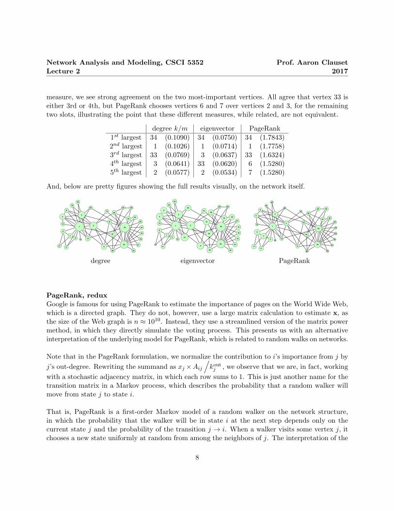
measure, we see strong agreement on the two most-important vertices. All agree that vertex 33 iseither 3rd or 4th, but PageRank chooses vertices 6 and 7 over vertices 2 and 3, for the remainingtwo slots, illustrating the point that these different measures, while related, are not equivalent.

degree k/m eigenvector PageRank

1st largest 34 (0.1090) 34 (0.0750) 34 (1.7843)2nd largest 1 (0.1026) 1 (0.0714) 1 (1.7758)3rd largest 33 (0.0769) 3 (0.0637) 33 (1.6324)4th largest 3 (0.0641) 33 (0.0620) 6 (1.5280)5th largest 2 (0.0577) 2 (0.0534) 7 (1.5280)

And, below are pretty figures showing the full results visually, on the network itself.

1

2

3

4

5

6

7

8

9

10

11

13

14

15

16

17

18

19

20

21

22

23

24

25 26

27

28

29

30

31

32

33

34

12

1

2

3

4

5

6

7

8

9

10

11

13

14

15

16

18

19

20

21

22

23

24

27

28

29

30

31

32

33

34

12

17

25 26

1

2

3

4

5

6

7

8

911

17

24

25 26

28

30

32

33

34

12

10

13

14

15

16

18

19

20

21

22

23

27

29

31

degree eigenvector PageRank

PageRank, reduxGoogle is famous for using PageRank to estimate the importance of pages on the World Wide Web,which is a directed graph. They do not, however, use a large matrix calculation to estimate x, asthe size of the Web graph is n ≈ 1010. Instead, they use a streamlined version of the matrix powermethod, in which they directly simulate the voting process. This presents us with an alternativeinterpretation of the underlying model for PageRank, which is related to random walks on networks.

Note that in the PageRank formulation, we normalize the contribution to i’s importance from j by

j’s out-degree. Rewriting the summand as xj ×Aij

/koutj , we observe that we are, in fact, working

with a stochastic adjacency matrix, in which each row sums to 1. This is just another name for thetransition matrix in a Markov process, which describes the probability that a random walker willmove from state j to state i.

That is, PageRank is a first-order Markov model of a random walker on the network structure,in which the probability that the walker will be in state i at the next step depends only on thecurrent state j and the probability of the transition j → i. When a walker visits some vertex j, itchooses a new state uniformly at random from among the neighbors of j. The interpretation of the

8



constant term α in the above formulation is a “teleportation” probability, i.e., with probability α,the random walker follows the Markov processes; otherwise, it chooses a uniformly random vertexto move to.

When α is large, the Markov process dominates, and the random walker tends to walk along thenetwork’s edges. When the walker enters a part of the network with few out-going edges, theteleportation probability allows the walk to restart somewhere else. On the World Wide Web, thisprocess is crucial, as the strongly connected component of the web graph is only a modest portionof the entire graph, and Google would not be useful if its “web crawlers” were constantly gettingstuck in obscure corners of the graph.

The streamlined matrix power method Google used to calculate PageRank essentially directlysimulates these random walkers, having each vertex repeatedly vote for its neighbors in proportionto its current centrality divided by its out-degree.

3 Geometric centrality

Another class of centrality measures takes a geometric approach to identifying important vertices,relying on geodesic paths between pairs of vertices. Notably, geodesic distances are not metric—they do not obey the triangle inequality—which means applying our (Euclidean) intuition mayprovide incorrect interpretations of the results. In many cases, the most central vertices underthese measures are completely different from those identified by degree-based measures. Here wewill study closeness and betweenness centrality scores. As a final point, we note that there are anumber of other centrality measures to be found in the literature—and some are even used to studyreal networks—but the ones we have covered here represent the most common ones.

3.1 Centrality by closeness

A literal interpretation of “centrality” takes inspiration from geometry: the most central point ina k-dimensional body has short paths—it is the point closest—to all other points in the body. Ifdij denotes the geodesic distance between vertices i and j, then the average distance from i to allother vertices10 is given by

`i =1

n

n∑j=1

dij . (6)

10Sometimes researchers use a summation that omits the path from i to i, which is a geodesic path of length zero,in which case we replace n by n − 1 in Eq. (6). However, this choice simply rescales all mean distances by a factorof n/(n− 1), which cannot change the relative ordering. Eq. (6) is a more convenient mathematical form, and thuswe employ it here.

9



This quantity is large for peripheral vertices, i.e., those far from most other vertices, and smallfor central vertices, i.e., those close to other vertices. This pattern runs in the opposite directionof most other centrality measures, which are large for central vertices and small for non-centralvertices. Thus, the closeness centrality of vertex i is typically defined as its inverse:

Ci =1

`i=

n∑nj=1 dij

. (7)

There are two practical problems with this definition. First, most networks have small diameters(being roughly log n), and thus the range of values that Ci assumes is fairly narrow. Small varia-tions in network topology, perhaps generated by a few missing edges, will produce large changesin a relative ordering. Second, closeness cannot be calculated for a network that is not a singlestrongly connected component, e.g., an undirected network with only one component. A pair ofnodes in distinct components have, by definition, a geodesic distance of dij = ∞, which results inCi = 0.11 As a result, closeness may only be used in specific contexts.

Harmonic centralityAn elegant solution to several of these problems, sometimes called the harmonic centrality, is totake the harmonic mean of the geodesic distances from i:

Ci =1

n− 1

∑j(6=i)

1

dij, (8)

where dij =∞ if there is no path between i and j and we exclude the term dii = 0 to prevent the sumfrom diverging for trivial reasons. This formulation naturally handles disconnected components, asthe dij =∞ terms contribute 0 to the sum; it also has several other nice mathematical properties.12

The calculation of harmonic centrality may be done efficiently using any standard single-sourceshortest-paths (SSSP) algorithm. For undirected graphs, a breadth first search forest is sufficient,while for directed or weighted graphs, Dijkstra’s algorithm works well. In either case, only theactual distances (number of edges) need be retained, rather than the paths themselves.

For example, consider the following small network. The highlighted vertex has a path of length 0 toitself, paths of lengths {1, 2, 2, 2, 2, 2} to the vertices in the clique on the right, and paths of lengths{1, 1, 2, 2, 3} to the vertices in the cycle on the left. Its closeness centrality is thus 12/20 = 0.6,

11Some researchers have attempted to fix this latter problem by only averaging over distances to vertices in thesame component as i, but this introduces a new problem, in which a vertex in a small component, which generallyare considered genuinely peripheral, can have a closeness score comparable to that of an important vertex in a largecomponent.

12For a detailed explanation, see P. Boldi and S. Vigna, “Axioms for Centrality.” Preprint, arxiv:1308.2140

(2013).

10



which is the maximal score in the network, but one other vertex has the same closeness (whichone?). Its harmonic centrality is 0.6212 . . . , which is the second largest value (what is the largest?).The minimal scores are 0.316 (closeness) and 0.417 (harmonic), which illustrates the narrow rangeof variation of closeness (less than a factor of 2). (Do you see which vertex produces these scores?)

Applying the harmonic centrality calculation to the karate club network yields the figure on thenext page (with circle size scaled to be proportional to the score). The small size of this networktends to compress the centrality scores into a narrow range. Comparing the harmonic scores todegrees, we observe several differences. For instance, the centrality of vertex 17, the only vertex ingroup 1 that does not connect to the hub vertex 1, is lower than that of vertex 12, which has thelowest degree but connects to the high-degree vertex 1. And, vertex 3 has a harmonic centralityclose to that of the main hubs 1 and 34, by virtue of it being “between” the two groups and thushaving short paths to all members of each.

1

2

3

4

5

6

7

8

9

10

11

13

14

15

16

17

18

19

20

21

22

23

24

25 26

27

28

29

30

31

32

33

34

12

1

2

3

4

5

6

7

8

9

10

11

14

15

16

18

19

20

21

22

23

24

28

29

30

31

32

33

34

12

13

17

25 26

27

degree harmonic

Relationship to degree-based centralitiesIn fact, degree-based centrality measures are related to geodesic-based measures like closeness andharmonic centrality, although they do emphasize different aspects of network structure. For in-

11



stance, the Katz centrality can be seen as a weighted sum of all paths of different lengths to avertex i (weighted so that the summation converges), while PageRank can be viewed as a sum ofrandom paths on the network that touch i (recall the Markov model or “random surfer” interpreta-tion). Both of these scores are measuring different paths of different types than the geodesic-basedmeasures, which assume that only the shortest-path is relevant, but they can be viewed as path-based measures nevertheless. As a result, we can expect these measures to be correlated for certaintypes of networks, as we will see below.

3.2 Centrality by betweenness

Our final measure of importance is also derived from geodesic paths, and relies on the notion thatimportant vertices are the “bridges” over which information tends to flow. This idea is based,in part, on a seminal paper by Mark Granovetter called “The strength of weak ties”13 in whichit was shown that most job seekers (who participated in the study) found their ultimate employ-ment through a weak tie, that is, through an acquaintance, rather than a strong tie or a close friend.

The theoretical argument for this pattern was that the information residing at either end of a strongtie is nearly identical because these vertices frequently exchange what information they have. Thus,you and your friends are mostly aware of the same job opportunities, which, had you been qualifiedfor them, you would not be still seeking a job. In contrast, weak ties synchronize their informationmore rarely, and thus serve as greater sources of novel information when such information is needed.That is, your acquaintances are more likely to know about jobs you have not already considered.

The implication is that vertices that serve as information bridges for many pairs of other verticesare important. Let us make the unrealistic assumption that each pair of vertices exchanges infor-mation as a constant rate, and that information is passed along geodesic paths on the network (i.e.,information always follows the shortest path between two points). The number of these geodesicpaths that cross some vertex i is thus a measure of its importance for synchronizing informationacross the network, and this is precisely what we call betweenness centrality. There are severaldifferent mathematical definitions of betweenness, and we will cover the main ones here.14

Our first definition of betweenness is to simply count the number of geodesics that pass through a

13In American Journal of Sociology 78, 1360–1380 (1973).14Some of the variations observed in the literature, particularly the sociology literature, differ only in a multiplicative

or additive constant to all scores. These constants cannot alter the relative ordering of vertices, and thus here weprefer the more mathematically simple forms.

12



particular vertex i:

bi =∑jk

#{geodesic paths j → · · · → i→ · · · → k}

=∑jk

σjk(i) , (9)

where σjk(i) denotes the number of paths from j → k that pass through i. Note that applied to anundirected network, this definition double counts each path, once for the j → k direction and oncefor the k → j direction. This behavior is not an issue, however, as multiplication by a constantdoes not alter the final ordering. Furthermore, this definition includes paths from j to k = j. Thistoo simply adds a constant to each centrality score, which does not alter the final ordering.

A second definition of betweenness divides each count by the number of possible geodesics fromj → k:

bi =∑jk

#{geodesic paths j → · · · → i→ · · · → k}#{geodesic paths j → · · · → k}

=∑jk

σjk(i)

σjk, (10)

where σjk counts all the geodesic paths j → k, not just those that pass through i, and where wedefine 0/0 = 0 for disconnected pairs of vertices. This version has the nice feature that if thereare multiple geodesic paths from j → k, some of which pass through i and others of which passthrough `, both i and ` get equal credit for each path.

Finally, a third definition normalizes Eq. (10) to fall on the unit interval [0, 1] by dividing by thenumber of pairs in the network:

bi =1

n2

∑jk

σjk(i)

σjk. (11)

For example, consider again our small network of a clique and a cycle. The highlighted vertex lieson every geodesic between the left and right groups, of which there are 72. (Why 72?) It alsolies on every geodesic path from it to other vertices in the left group, of which there are 6. Thus,the first definition of betweenness would yield b◦ = 78. One of the vertices in the cycle has twogeodesic paths to each of the vertices in the clique plus the highlighted vertex (and vice versa);however, both pass through the highlighted vertex, and so the corresponding term in Eq. (10) is1, as before. All other pairs of vertices have a unique geodesic path, and thus the second defi-nition of betweenness also yields b◦ = 78. Finally, the third definition divides this value by n2,

13



yielding b◦ = 78/144 ≈ 0.542. In each of the three definitions, this score is the maximal value,making the highlighted vertex the most central. The minimal scores are achieved by only onevertex (which one?), and are b• = 23 (being 2n − 1; why is this the lower bound?), b• = 23, andb• = 23/144 ≈ 0.160 (about 3.4 times smaller than the maximum value).

To compute betweenness for an arbitrary network requires enumerating the geodesic paths betweenall pairs of vertices in the network; this can be done naıvely in O(n3) time and O(n2) space.15 Arough approximation to betweenness may be calculated by solving the SSSP problem once for eachvertex and then counting the number of times a vertex i appears in any of the resulting search trees.This procedure takes O(n(n+m)) time for unweighted networks, using a breadth-first search forest,and O(n(m + n log n)) for weighted networks, using Dijkstra’s algorithm with a Fibonacci heap.However, this approach makes errors whenever there are multiple geodesics between some j and k,a situation that is common in unweighted networks. In this event, full weight will be assigned to thevertices along only one of the geodesics rather than dividing that weight evenly across all of them.16

Applied to the karate club, the figures on the following page illustrate that betweenness assignsmuch smaller relative scores to a greater portion of the network than we saw in degree or harmoniccentrality. The most between vertices are still the high-degree nodes (1, 33 and 34), mainly becausethese nodes are the “brokers” for many other nodes’ access to the rest of the network. Verticesthat lay between the two groups, like 3 and 32, also receive relatively high betweenness for similarreasons.

15It can be done faster, however, using the accumulation algorithm described in U. Brandes, “A Faster Algorithm forBetweenness Centrality.” Journal of Mathematical Sociology 25(2), 163–177 (2001). This algorithm takes O(n + m)space, and O(nm) time for unweighted networks or O(nm + n2 logn) time for weighted networks.

16We may sidestep such a tie-breaking problem by adding a small amount of noise to each edge weight. Withhigh probability, this perturbed network will have a unique geodesic path between each pair of vertices, and eachperturbation chooses that geodesic uniformly at random from the original set. (Alternatively, if the network is storedas an adjacency list, we may simply randomly permute the ordering of each vertex’s adjacencies.) For up to moderate-sized networks, we can use this trick to enumerate all geodesic paths by repeating the following process: perturb theedge weights, run the SSSP algorithm from each vertex, take the union of the identified geodesics with those of thepast step.

14



The following table compares the relative rankings derived from the different measures defined inthis lecture, along with a ranking by degree, for the top few most central vertices. (The last col-umn gives the betweenness estimated by using only a single SSSP tree from each vertex, in orderto illustrate the differences this approximation produces.) A few details are worth pointing out.For instance, closeness scores are all very similar, differing only in their second decimal place, whileother scores have greater variability, with betweenness having the broadest range. Although allmeasures generally agree on which vertices are among the most important (mainly 1, 3, 32 and34), they disagree on the precise ordering of their importance. Consider applying these measuresto a novel network: how would such disagreements complicate your interpretation of which verticesare most important? what if there were more disagreement about which vertices were in the top five?

degree k/m closeness harmonic betweenness betweenness∗

Eq. (7) Eq. (8) Eq. (11) Eq. (11)

1st largest 34 (0.1090) 1 (0.5862) 34 (0.7045) 1 (0.4577) 1 (0.4939)2nd largest 1 (0.1026) 3 (0.5763) 1 (0.7020) 34 (0.3357) 34 (0.2708)3rd largest 33 (0.0769) 34 (0.5667) 3 (0.6364) 33 (0.1906) 32 (0.2638)4th largest 3 (0.0641) 32 (0.5574) 33 (0.6338) 3 (0.1892) 33 (0.2439)5th largest 2 (0.0577) 9 (0.5312) 32 (0.5859) 32 (0.1843) 3 (0.1912)

1

2

3

4

5

6

7

8

9

10

11

13

14

15

16

17

18

19

20

21

22

23

24

25 26

27

28

29

30

31

32

33

34

12

1

2

3

4

5

6

7

8

9

32

33

34

12

13

17

25 26

27

10

11

14

15

16

19

21

23

22

1820

24

28

29

30

31

degree betweenness

Finally, we return to the question of correlation between measures, as both harmonic and between-ness centrality are functions of geodesic paths, which may produce correlated rankings. On theother hand, such a correlation is not a foregone conclusion. Consider a vertex v that has only asingle connection to another, highly central vertex. This vertex would have a minimal betweennessscore, as it lies on no geodesic paths that do not begin or terminate at v, but its path lengthsare all very short, being a single step longer than the paths to the highly central node to which itconnects. Thus, v would have high closeness or harmonic centrality, but low betweenness.

15



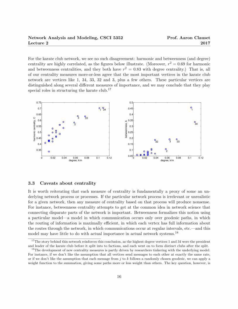
For the karate club network, we see no such disagreement: harmonic and betweenness (and degree)centrality are highly correlated, as the figures below illustrate. (Moreover, r2 = 0.69 for harmonicand betweenness centralities, and they both have r2 = 0.83 with degree centrality.) That is, allof our centrality measures more-or-less agree that the most important vertices in the karate clubnetwork are vertices like 1, 34, 33, 32 and 3, plus a few others. These particular vertices aredistinguished along several different measures of importance, and we may conclude that they playspecial roles in structuring the karate club.17

0 0.02 0.04 0.06 0.08 0.1 0.12

0.35

0.4

0.45

0.5

0.55

0.6

0.65

0.7

0.75

341

333

2

degree, k/m

ha

rmo

nic

ce

ntr

alit

y,

C

0 0.02 0.04 0.06 0.08 0.1 0.120.05

0.1

0.15

0.2

0.25

0.3

0.35

0.4

0.45

0.5

34

1

333

2

32

degree, k/m

be

twe

en

ne

ss,

b

3.3 Caveats about centrality

It is worth reiterating that each measure of centrality is fundamentally a proxy of some an un-derlying network process or processes. If the particular network process is irrelevant or unrealisticfor a given network, then any measure of centrality based on that process will produce nonsense.For instance, betweenness centrality attempts to get at the common idea in network science thatconnecting disparate parts of the network is important. Betweenness formalizes this notion usinga particular model—a model in which communication occurs only over geodesic paths, in whichthe routing of information is maximally efficient, in which each vertex has full information aboutthe routes through the network, in which communications occur at regular intervals, etc.—and thismodel may have little to do with actual importance in actual network systems.18

17The story behind this network reinforces this conclusion, as the highest degree vertices 1 and 34 were the presidentand leader of the karate club before it split into to factions, and each went on to form distinct clubs after the split.

18The development of new centrality measures is partly driven by researchers tinkering with the underlying model.For instance, if we don’t like the assumption that all vertices send messages to each other at exactly the same rate,or if we don’t like the assumption that each message from j to k follows a randomly chosen geodesic, we can apply aweight function to the summation, giving some paths more or less weight than others. The key question, however, is

16



This does not mean that centrality measures cannot or should not be used. Rather, they should beused mainly in an exploratory manner, to gain some insight into the general structure and patternof a network and to generate hypotheses about what processes might have generated that structure.These measures may also serve the useful purpose of building our intuition about what kinds ofstructural patterns correlate with other types of structural patterns, a topic we will revisit whenwe study random graph models.

As a nice visualization, here’s an image by Claudio Rocchini on the Wikipedia page for centralities,which shows how different centrality measures think different vertices are more or less important.Do you see why?

Figure 1: An example calculation by Claudio Rocchini (from the Wikipedia page on Centrality) of(A) degree centrality, (B) closeness centrality, (C) betweenness centrality, (D) eigenvector centrality,(E) katz centrality and (F) alpha centrality.

whether or now such a variation provides more useful insights for some system than existing measures.

17



4 At home

1. Read Chapter 7.1–7.5 (pages 168–181) in Networks (degree centralities)

2. Read Chapter 7.6–7.8 (pages 181–198) in Networks (geometric centralities)

3. Optional reading: P. Boldi and S. Vigna, “Axioms for Centrality.” Preprint, arxiv:1308.2140(2013).

18

1 Structural importance - Santa Fe...

Documents

Transcript of 1 Structural importance - Santa Fe...