1 STAT 552 PROBABILITY AND STATISTICS II INTRODUCTION Short review of S551.
51
1 STAT 552 PROBABILITY AND STATISTICS II INTRODUCTION Short review of S551
-
Upload
julie-robbins -
Category
Documents
-
view
224 -
download
0
Transcript of 1 STAT 552 PROBABILITY AND STATISTICS II INTRODUCTION Short review of S551.

1
STAT 552PROBABILITY AND
STATISTICS II
INTRODUCTIONShort review of S551

2
WHAT IS STATISTICS?
• Statistics is a science of collecting data,
organizing and describing it and drawing
conclusions from it. That is, statistics is
a way to get information from data. It is
the science of uncertainty.

3
BASIC DEFINITIONS
• POPULATION: The collection of all items of interest in a particular study.
•VARIABLE: A characteristic of interest about each
element of a population or sample.
•STATISTIC: A descriptive measure of a sample
•SAMPLE: A set of data drawn from the population;
a subset of the population available for observation
•PARAMETER: A descriptive measure of the
population, e.g., mean

STATISTIC
• Statistic (or estimator) is any function of a r.v. of r.s. which do not contain any unknown quantity. E.g.o are statistics.
o are NOT.
• Any observed or particular value of an estimator is an estimate.
4
)X(xam),X(nim,n/X,X,X ii
ii
n
1ii
n
1i
n
1iii
n
1ii
n
1ii /X,X

5
• The set of all possible outcomes of an experiment is called a sample space and denoted by S.
• Determining the outcomes.– Build an exhaustive list of all possible
outcomes.– Make sure the listed outcomes are mutually
exclusive.
Sample Space

RANDOM VARIABLES• Variables whose observed value is determined
by chance• A r.v. is a function defined on the sample space
S that associates a real number with each outcome in S.
• Rvs are denoted by uppercase letters, and their observed values by lowercase letters.
6

7
DESCRIPTIVE STATISTICS
• Descriptive statistics involves the arrangement, summary, and presentation of data, to enable meaningful interpretation, and to support decision making.
• Descriptive statistics methods make use of– graphical techniques– numerical descriptive measures.

Types of data – examplesExamples of types of data
Quantitative
Continuous Discrete
Blood pressure, height, weight, age
Number of childrenNumber of attacks of asthma per week
Categorical (Qualitative)
Ordinal (Ordered categories) Nominal (Unordered categories)
Grade of breast cancerBetter, same, worseDisagree, neutral, agree
Sex (Male/female)Alive or deadBlood group O, A, B, AB
8

9
POPULATION SAMPLE
PROBABILITY
STATISTICAL INFERENCE
10
• PROBABILITY: A numerical value
expressing the degree of uncertainty regarding the occurrence of an event. A measure of uncertainty.
• STATISTICAL INFERENCE: The science of drawing inferences about the population based only on a part of the population, sample.

Probability
P : S [0,1]
Probability domain range
function
11

12
THE CALCULUS OF PROBABILITIES
• If P is a probability function and A is any
set, then
a. P()=0
b. P(A) 1
c. P(AC)=1 P(A)

13
ODDS• The odds of an event A is defined by
( ) ( )( ) 1 ( )C
P A P AP A P A
•It tells us how much more likely to see the occurrence of event A.

ODDS RATIO
• OR is the ratio of two odds.
• Useful for comparing the odds under two different conditions or for two different groups, e.g. odds for males versus females.
14

CONDITIONAL PROBABILITY
• (Marginal) Probability: P(A): How likely is it that an event A will occur when an experiment is performed?
• Conditional Probability: P(A|B): How will the probability of event A be affected by the knowledge of the occurrence or nonoccurrence of event B?
• If two events are independent, then P(A|B)=P(A)
15

CONDITIONAL PROBABILITY
16
1)|(0
0)()(
)(B)|P(A
BAP
BPifBP
BAP
)|()()|()()( BAPBPABPAPABP
),...,|()...,|()|()()...( 1121312121 nnn AAAPAAAPAAPAPAAAP

BAYES THEOREM
• Suppose you have P(B|A), but need P(A|B).
17
0)B(Pfor)B(P
)A(P)A|B(P
)B(P
)BA(P)B|A(P

Independence• A and B are independent iff
– P(A|B)=P(A) or P(B|A)=P(B)– P(AB)=P(A)P(B)
• A1, A2, …, An are mutually independent iff
for every subset j of {1,2,…,n}
E.g. for n=3, A1, A2, A3 are mutually independent iff P(A1A2A3)=P(A1)P(A2)P(A3) and P(A1A2)=P(A1)P(A2) and P(A1A3)=P(A1)P(A3) and P(A2A3)=P(A2)P(A3)
18
ji
iji
i APAP )()(

DISCRETE RANDOM VARIABLES
• If the set of all possible values of a r.v. X is a countable set, then X is called discrete r.v.
• The function f(x)=P(X=x) for x=x1,x2, … that assigns the probability to each value x is called probability density function (p.d.f.) or probability mass function (p.m.f.)
19

Example
• Discrete Uniform distribution:
• Example: throw a fair die. P(X=1)=…=P(X=6)=1/6
20
,...2,1N;N,...,2,1x;N
1)xX(P

CONTINUOUS RANDOM VARIABLES
• When sample space is uncountable (continuous)
• Example: Continuous Uniform(a,b)
21
.bxaab
1)X(f
CUMULATIVE DENSITY FUNCTION (C.D.F.)
• CDF of a r.v. X is defined as F(x)=P(X≤x).
22

JOINT DISCRETE DISTRIBUTIONS
• A function f(x1, x2,…, xk) is the joint pmf for some vector valued rv X=(X1, X2,…,Xk) iff the following properties are satisfied:
f(x1, x2,…, xk) 0 for all (x1, x2,…, xk)
and
23
.1x,...,x,xf...
1x kxk21

MARGINAL DISCRETE DISTRIBUTIONS
• If the pair (X1,X2) of discrete random variables has the joint pmf f(x1,x2), then the marginal pmfs of X1 and X2 are
24
12
21222111xx
xxfxf and xxfxf ,,

CONDITIONAL DISTRIBUTIONS
• If X1 and X2 are discrete or continuous random variables with joint pdf f(x1,x2), then the conditional pdf of X2 given X1=x1 is defined by
• For independent rvs,
25
elsewhere. 0 f that such ,0xx,xf
x,xfxxf 11
1
2112
.
.
121
212
xfxxf
xfxxf

26
EXPECTED VALUESLet X be a rv with pdf fX(x) and g(X) be a
function of X. Then, the expected value (or the mean or the mathematical expectation) of g(X)
Xx
X
g x f x , if X is discrete
E g Xg x f x dx, if X is continuous
providing the sum or the integral exists, i.e.,<E[g(X)]<.

27
EXPECTED VALUES
• E[g(X)] is finite if E[| g(X) |] is finite.
Xx
X
g x f x < , if X is discrete
E g Xg x f x dx< , if X is continuous

28
Laws of Expected Value E(c) = c E(X + c) = E(X) + c E(cX) = cE(X)
Laws of Variance V(c) = 0 V(X + c) = V(X) V(cX) = c2V(X)
Laws of Expected Value and Variance
Let X be a rv and c be a constant.

EXPECTED VALUE
29
.
k
iii
k
iii XEaXaE
11
If X and Y are independent,
YhEXgEYhXgE
The covariance of X and Y is defined as
)Y(E)X(E)XY(E
YEYXEXEY,XCov

EXPECTED VALUE
30
If X and Y are independent,
0YXCov ,
The reverse is usually not correct! It is only correct under normal distribution.
If (X,Y)~Normal, then X and Y are independent iff
Cov(X,Y)=0

EXPECTED VALUE
31
212121 2 XXCovXVarXVarXXVar ,
If X1 and X2 are independent,
2121 XVarXVarXXVar

CONDITIONAL EXPECTATION AND VARIANCE
32
.continuous are Y and X if , dyxyyf
discrete. are Y and X if , xyyf
xYEy
22 xYExYExYVar

CONDITIONAL EXPECTATION AND VARIANCE
33
YEXYEE
))X|Y(E(Var))X|Y(Var(E)Y(Var XX
(EVVE rule)
Proofs available in Casella & Berger (1990), pgs. 154 & 158

34
SOME MATHEMATICAL EXPECTATIONS
• Population Mean: = E(X)
• Population Variance:
2 22 2 0Var X E X E X
(measure of the deviation from the population mean)
• Population Standard Deviation: 2 0
• Moments:* kk E X the k-th moment
k
k E X the k-th central moment

35
This measure reflects the dispersion of all the observations
The variance of a population of size N x1, x2,…,xN
whose mean is is defined as
The variance of a sample of n observationsx1, x2, …,xn whose mean is is defined asx
N
)x( 2i
N1i2
N
)x( 2i
N1i2
1n
)xx(s
2i
n1i2
1n
)xx(s
2i
n1i2
The Variance
n
xx
ns i
ni
i
n
i
212
1
2 )(
1
1
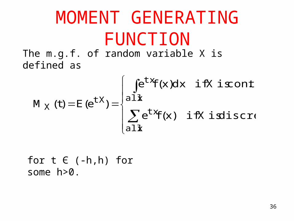
MOMENT GENERATING FUNCTION
36
xall
tx
xall
tx
tXX
discreteisXif)x(fe
.contisXifdx)x(fe
)e(E)t(M
The m.g.f. of random variable X is defined as
for t Є (-h,h) for some h>0.

Properties of m.g.f.
• M(0)=E[1]=1
• If a r.v. X has m.g.f. M(t), then Y=aX+b has a m.g.f.
•
• M.g.f does not always exists (e.g. Cauchy distribution)
37
)at(Mebt
.derivativektheisMwhere)0(M)X(E th)k()k(k

CHARACTERISTIC FUNCTION
38
xall
itx
xall
itx
itXX
discreteisXifxfe
contisXifdxxfe
eEt)(
.)(
)()(
The c.h.f. of random variable X is defined as
for all real numbers t. 1,12 ii
C.h.f. always exists.

Uniqueness
Theorem:
1.If two r.v.s have mg.f.s that exist and are equal, then they have the same distribution.
2.If two r.v.s have the same distribution, then they have the same m.g.f. (if they exist)
Similar statements are true for c.h.f.
39

SOME DISCRETE PROBABILITY DISTRIBUTIONS
• Please review: Degenerate, Uniform, Bernoulli, Binomial, Poisson, Negative Binomial, Geometric, Hypergeometric, Extended Hypergeometric, Multinomial
40

SOME CONTINUOUS PROBABILITY DISTRIBUTIONS
• Please review: Uniform, Normal (Gaussian), Exponential, Gamma, Chi-Square, Beta, Weibull, Cauchy, Log-Normal, t, F Distributions
41

42
TRANSFORMATION OF RANDOM VARIABLES
• If X is an rv with pdf f(x), then Y=g(X) is also an rv. What is the pdf of Y?
• If X is a discrete rv, replace Y=g(X) whereever you see X in the pdf of f(x) by using the relation .
• If X is a continuous rv, then do the same thing, but now multiply with Jacobian.
• If it is not 1-to-1 transformation, divide the region into sub-regions for which we have 1-to-1 transformation.
)y(gx 1

CDF method
• Example: Let
Consider . What is the p.d.f. of Y?
• Solution:
43
0xfore1)x(F x2
XeY
1yfory2)y(Fdy
d)y(f
1yfory1)y(lnF
)ylnX(P)ye(P)yY(P)y(F
3YY
2X
XY

M.G.F. Method
• If X1,X2,…,Xn are independent random variables with MGFs Mxi (t), then the MGF of is
44
n
1iiXY )t(M)...t(M)t(M nX1XY

45
THE PROBABILITY INTEGRAL TRANSFORMATION
• Let X have continuous cdf FX(x) and define the rv Y as Y=FX(x). Then,
Y ~ Uniform(0,1), that is,
P(Y y) = y, 0<y<1.
• This is very commonly used, especially in random number generation procedures.
SAMPLING DISTRIBUTION
• A statistic is also a random variable. Its distribution depends on the distribution of the random sample and the form of the function Y=T(X1, X2,…,Xn). The probability distribution of a statistic Y is called the sampling distribution of Y.

47
SAMPLING FROM THE NORMAL DISTRIBUTION
Properties of the Sample Mean and Sample Variance
• Let X1, X2,…,Xn be a r.s. of size n from a N(,2) distribution. Then,
2) and are independent rvs.a X S
2) ~ , /b X N n
22
12
1) ~ n
n Sc

48
SAMPLING FROM THE NORMAL DISTRIBUTION
If population variance is unknown, we use sample variance:

49
SAMPLING FROM THE NORMAL DISTRIBUTION
• The F distribution allows us to compare the variances by giving the distribution of
2 2 2 2
1, 12 2 2 2
/ /~
/ /X Y X X
n m
X Y Y Y
S S SF
S
• If X~Fp,q, then 1/X~Fq,p.
• If X~tq, then X2~F1,q.

50
CENTRAL LIMIT THEOREMIf a random sample is drawn from any population, the
sampling distribution of the sample mean is approximately normal for a sufficiently large sample size. The larger the sample size, the more closely the sampling distribution of will resemble a normal distribution.
Random Sample
(X1, X2, X3, …,Xn)
Sample Mean Distribution
XX
Random Variable (Population) Distribution
as n
X

51
Sampling Distribution of the Sample Mean
If X is normal, is normal.
If X is non-normal, is approximately normally distributed for sample size greater than or equal to 30.
X
2
2 or X Xn n
X
X
2 XX ~ N( , / n ) Z ~ N(0,1)
/ n


![Federal Coal Mine Safety Act of 1952 - GPO stat.] public law 552-july 16, 1952](https://static.fdocuments.net/doc/165x107/5ac0bdd87f8b9a5a4e8c5d89/federal-coal-mine-safety-act-of-1952-gpo-stat-public-law-552-july-16-1952.jpg)