1

Specific Factors and

Income Distribution

© Prof. J. Peter Neary 2009

Economics Department, Oxford

2

Specific-Factors Model

Ricardian model has nothing to say about domestic income distribution

BUT: In reality, trade has important effects on distribution

One major reason: Factors cannot move immediately or costlessly between sectors

An interesting alternative model, which focuses clearly on this issue, is the Specific-Factors model

Difference in assumptions: 3 factors instead of 1

• Labour (L) is mobile between sectors

• Capital (K) and Land (T) are immobile or “sector-specific”

Similar to 2-sector Ricardian model in other respects:

• 2 goods: Manufacturing and Food

• Full Employment; perfect competition

3

Fig. 3-1: The Production Functionfor Manufactures

QM

LM

QM = QM(K, LM)

LM

MPLM

Fig. 3-2: The Marginal Productof Labour in Manufactures

• Equals the slope of the prod. func.• Downward-sloping: Reflecting

Diminishing Returns• As more labour is added to fixed

amount of capital, its marginal return falls

4Fig. 3-3: The PPF in the Specific-Factors Model

Full-Employment Locus:LM+LF=L

Production FunctionFor Manufactures

Production FunctionFor Food

PPF: ProductionPossibilityFrontier

QM

QF

LF

LM

Exercise: repeat this slide and last for 2-good Ricardian model

5

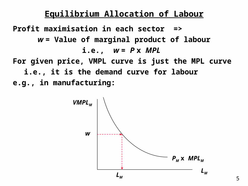
Equilibrium Allocation of Labour

Profit maximisation in each sector =>

w = Value of marginal product of labour

i.e., w = P x MPL

For given price, VMPL curve is just the MPL curve

i.e., it is the demand curve for labour

e.g., in manufacturing:

LM

VMPLM

w

LM

PM x MPLM

6

Equilibrium Allocation of Labour (cont.)

Similarly in food:

LF

VMPLF

w

LF

LFLF

VMPLF

Now, flip this diagram around:

w

7

Equilibrium Allocation of Labour (cont.)

Finally, combine the two labour demand curves:

LM

VMPLF

w

LFLM

VMPLM

Horizontal axis measures L: i.e., full employment

Intersection of two demand curves determines equilibrium wage and allocation of labour between sectors

Note: w is exogenous in partial equilibrium, endogenous in general equilibrium: follow the arrows!

LF

L

8

Effects of a Rise in the Relative Price of Manufactures

LM

VMPLF

w

LFLM

VMPLM

Curve shifts upwards: equilibrium shifts from A to B• Employment and hence output of manufactures increase (intuitive)

• Wage rises BUT by less than the price increase

• i.e., wage-earners gain in terms of food, lose in terms of manufactures

• Owners of capital gain, owners of land lose (in terms of both goods)

LF

A

B

9

Effects of price rise in PPF diagram:• Initial equilibrium at A

• Price = MC in each sector => slope of price line = slope of PPF

Effects of a Rise in the Relative Price of Manufactures (cont.)

Higher world price of M => steeper price line

QM

QF

A

B

=> New equilibrium at B: QM rises, QF falls

10

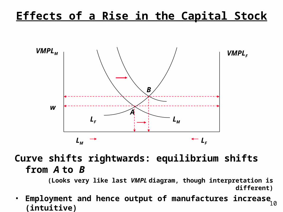
Effects of a Rise in the Capital Stock

LM

VMPLF

w

LFLM

VMPLM

Curve shifts rightwards: equilibrium shifts from A to B(Looks very like last VMPL diagram, though interpretation is different)

• Employment and hence output of manufactures increase (intuitive)

• Wage rises relative to both goods prices: i.e., wage-earners definitely gain

• Owners of capital lose per unit, owners of land lose

LF

A

B

11

p=pM/pF

Q Q

Q QM M

F F

*

*

World supply curvean average of the two

Foreign has less capital:So lower relative supply of M

Relative demand curvedetermines equilibrium

in both autarky and free trade

Assume Home has more capital:So higher relative supply of M

Implications for Trade Patterns

p*A

pA

pF

N.B. This diagram is similar to the 2-good Ricardian case; differences:• Countries have identical technology, and differ in factor endowments • The supply curves are smooth

12

Distributional Conflict versus Aggregate Gains

Move from autarky at A to free trade at B:

QM

QF

A

B

• Since some factors gain and some lose, what can we say?

• At least, we can say that the economy as a whole could do better than its initial total consumption

i.e., starting from B, economy could consume along red portion of new price line

• As in Ricardian model, trade expands the economy’s consumption possibilities

• So, losers could be compensated and still leave gainers better off

• BUT: In practice, compensation is rarely carried out

13

Specific Factors: General Conclusions

• Differences in resources: a source of comparative advantage[Topical, with oil at $120 a barrel! (April 2008)]

• Trade (and any other change) has both winners and losers

• Winners are factors specific to export sectors; losers are factors specific to import-competing sectors

• Winners could compensate losers …

• BUT: In practice, such compensation is rarely carried out fully

• Though there are examples of partial compensatione.g., adjustment assistance, retraining subsidies, temporary subsidies, etc.

• Case study: Repeal of the Corn Laws in 1846See: http://en.wikipedia.org/wiki/Corn_Laws

• Overall: A very neat, simple model:– Rationalises partial equilibrium intuition, in a fully specified GE model

– Highlights effects on distribution

– But: Naïve theory of trade [Samuelson: “tropical countries export tropical products because of the abundance of tropical products there”!]

14

Reconciling the HOS and Specific-Factors Models

– Note: There is a magnification effect on the rentals (though not on the wage)

– Compare this with the effects in the HOS model

FFMMFM rpwprpp ˆˆˆˆˆˆˆ

So far: Two interesting but very different models: Are they necessarily in conflict?

Not necessarily - One way of reconciling them: Interpret each as applying to a different time frame.

• SF: Describes short-run responses

• HOS: Describes longer-run responses (after capital stock has had time to adjust)

Mechanism driving this adjustment can be seen by looking at full effect of a price change in SF model:

15

Reconciling the HOS and Specific-Factors Models (cont.)

This rise in rM relative to rF encourages capital to flow (reallocate) over time out of sector F into sector M

As a result:

• Long-run response to price change is greater than short-run response: i.e., declining sector declines by more

• Economy converges in longer run towards the equilibrium predicted by the HOS model

Finally: An alternative (though related) difference in interpretation between the two models concerns the different kinds of shocks they illustrate:

• SF: Describes response to unanticipated shocks

• HOS: Describes response to anticipated shocks: Capital will have already begun to move