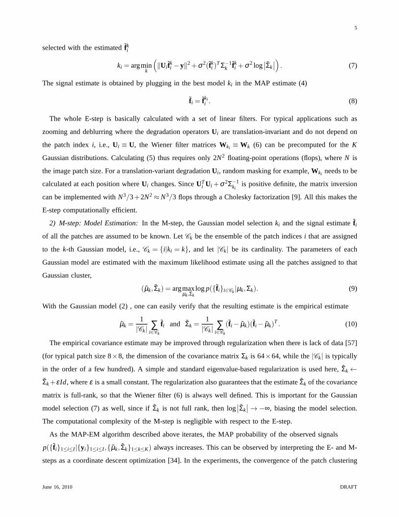
arX

iv:1

006.

3056

v1 [

cs.C

V]

15 J

un 2

010

1

Solving Inverse Problems with Piecewise LinearEstimators: From Gaussian Mixture Models to

Structured SparsityGuoshen YU*1, Guillermo SAPIRO1, and Stephane MALLAT 2

1ECE, University of Minnesota, Minneapolis, Minnesota, 55414, USA2CMAP, Ecole Polytechnique, 91128 Palaiseau Cedex, France

EDICS: TEC-RST

June 16, 2010

Abstract

A general framework for solving image inverse problems is introduced in this paper. The approach isbased on Gaussian mixture models, estimated via a computationally efficient MAP-EM algorithm. A dualmathematical interpretation of the proposed framework with structured sparse estimation is described, whichshows that the resulting piecewise linear estimate stabilizes the estimation when compared to traditionalsparse inverse problem techniques. This interpretation also suggests an effective dictionary motivated initial-ization for the MAP-EM algorithm. We demonstrate that in a number of image inverse problems, includinginpainting, zooming, and deblurring, the same algorithm produces either equal, often significantly better, orvery small margin worse results than the best published ones, at a lower computational cost.

I. INTRODUCTION

Image restoration often requires to solve an inverse problem. It amounts to estimate an imagef from a

measurement

y = Uf+w,

obtained through a non-invertible linear degradation operator U, and contaminated by an additive noise

w. Typical degradation operators include masking, subsampling in a uniform grid and convolution, the

corresponding inverse problems often named inpainting or interpolation, zooming and deblurring. Estimating

f requires some prior information on the image, or equivalently image models. Finding good image models

is therefore at the heart of image estimation.

Mixture models are often used as image priors since they enjoy the flexibility of signal description by as-

suming that the signals are generated by a mixture of probability distributions [49]. Gaussian mixture models

(GMM) have been shown to provide powerful tools for data classification and segmentation applications (see

for example [14], [30], [54], [58]), however, they have not yet been shown to generate state-of-the-art in a

general class of inverse problems. Ghahramani and Jordan have applied GMM for learning from incomplete

data, i.e., images degraded by a masking operator, and have shown good classification results, however, it

does not lead to state-of-the-art inpainting [31]. Portilla et al. have shown image denoising impressive results

June 16, 2010 DRAFT

2

by assuming Gaussian scale mixture models (deviating from GMM by assuming different scale factors in

the mixture of Gaussians) on wavelet representations [55],and have recently extended its applications on

image deblurring [32]. Recently, Zhou et al. have developedan nonparametric Bayesian approach using

more elaborated models, such as beta and Dirichlet processes, which leads to excellent results in denoising

and inpainting [71].

The now popular sparse signal models, on the other hand, assume that the signals can be accurately

represented with a few coefficients selecting atoms in some dictionary [45]. Recently, very impressive image

restoration results have been obtained with local patch-based sparse representations calculated with dictio-

naries learned from natural images [2], [23], [43]. Relative to pre-fixed dictionaries such as wavelets [45],

curvelets [11], and bandlets [46], learned dictionaries enjoy the advantage of being better adapted to the

images, thereby enhancing the sparsity. However, dictionary learning is a large-scale and highly non-convex

problem. It requires high computational complexity, and its mathematical behavior is not yet well understood.

In the dictionaries aforementioned, the actual sparse image representation is calculated with relatively

expensive non-linear estimations, such asl1 or matching pursuits [19], [22], [48]. More importantly, as

will be reviewed in Section III-A, with a full degree of freedom in selecting the approximation space (atoms

of the dictionary), non-linear sparse inverse problem estimation may be unstable and imprecise due to the

coherence of the dictionary [47].

Structured sparse image representation models further regularize the sparse estimation by assuming de-

pendency on the selection of the active atoms. One simultaneously selects blocks of approximation atoms,

thereby reducing the number of possible approximation spaces [4], [25], [26], [35], [36], [59]. These

structured approximations have been shown to improve the signal estimation in a compressive sensing context

for a random operatorU. However, for more unstable inverse problems such as zooming or deblurring,

this regularization by itself is not sufficient to reach state-of-the-art results. Recently some good image

zooming results have been obtained with structured sparsity based on directional block structures in wavelet

representations [47]. However, this directional regularization is not general enough to be extended to solve

other inverse problems.

This work shows that the Gaussian mixture models (GMM), estimated via an MAP-EM (maximum a

posteriori expectation-maximization) algorithm, lead toresults in the same ballpark as the state-of-the-

art in a number of imaging inverse problems, at a lower computational cost. The MAP-EM algorithm is

described in Section II. After briefly reviewing sparse inverse problem estimation approaches, a mathematical

equivalence between the proposed piecewise linear estimation (PLE) from GMM/MAP-EM and structured

sparse estimation is shown in Section III. This connection shows that PLE stabilizes the sparse estimation

with a structured learned overcomplete dictionary composed of a union of PCA (Principal Component

June 16, 2010 DRAFT

3

Analysis) bases, and with collaborative prior informationincorporated in the eigenvalues, that privileges in

the estimation the atoms that are more likely to be important. This interpretation suggests also an effective

dictionary motivated initialization for the MAP-EM algorithm. In Section IV we support the importance of

different components of the proposed PLE via some initial experiments. Applications of the proposed PLE

in image inpainting, zooming, and deblurring are presentedin sections V, VI, and VII respectively, and are

compared with previous state-of-the-art methods. Conclusions are drawn in Section VIII.

II. PIECEWISE L INEAR ESTIMATION

This section describes the Gaussian mixture models (GMM) and the MAP-EM algorithm, which lead to

the proposed piecewise linear estimation (PLE).

A. Gaussian Mixture Model

Natural images include rich and non-stationary content, whereas when restricted to local windows, image

structures appear to be simpler and are therefore easier to model. Following some previous works [2], [10],

[43], an image is decomposed into overlapping√

N×√

N local patches

yi = Ui f i +wi, (1)

whereUi is the degradation operator restricted to the patchi, yi, f i and wi are respectively the degraded,

original image patches and the noise restricted to the patch, with 1≤ i ≤ I , I being the total number of

patches. Treated as a signal, each of the patches is estimated, and their corresponding estimates are finally

combined and averaged, leading to the estimate of the image.

GMM describes local image patches with a mixture of Gaussiandistributions. Assume there existK

Gaussian distributionsN (µk,Σk)1≤k≤K parametrized by their meansµk and covariancesΣk. Each image

patchf i is independently drawn from one of these Gaussians with an unknown indexk, whose probability

density function is

p(f i) =1

(2π)N/2|Σki |1/2exp

(

−12(f i−µk)

TΣ−1ki(f i−µk)

)

. (2)

Estimatingf i1≤i≤I from yi1≤i≤I can then be casted into the following problems:

• Estimate the Gaussian parameters(µk,Σk)1≤k≤K, from the degraded datayi1≤i≤I .

• Identify the Gaussian distributionki that generates the patchi, ∀1≤ i ≤ I .

• Estimatef i from its corresponding Gaussian distribution(µki ,Σki ), ∀1≤ i ≤ I .

These problems are overall non-convex. The next section will present a maximum a posteriori expectation-

maximization (MAP-EM) algorithm that calculates a local-minimum solution [3].

June 16, 2010 DRAFT

4

B. MAP-EM Algorithm

Following an initialization, addressed in Section III-C, the MAP-EM algorithm is an iterative procedure

that alternates between two steps:

• In the E-step, assuming that the estimates of the Gaussian parameters(µk, Σk)1≤k≤K are known

(following the previous M-step), for each patch one calculates the maximum a posteriori (MAP)

estimatesfki with all the Gaussian models, and selects the best Gaussian modelki to obtain the estimate

of the patchf i = fkii .

• In the M-step, assuming that the Gaussian model selectionki and the signal estimatef i , ∀i, are known

(following the previous E-step), one estimates (updates) the Gaussian models(µk, Σk)1≤k≤K.

1) E-step: Signal Estimation and Model Selection:In the E-step, the estimates of the Gaussian parameters

(µk, Σk)1≤k≤K are assumed to be known. To simplify the notation, we assume without loss of generality

that the Gaussians have zero meansµk = 0, as one can always center the image patches with respect to the

means.

For each image patchi, the signal estimation and model selection is calculated tomaximize the log

a-posteriori probability logp(f i|yi , Σk):

(f i ,ki) = argmaxf,k

logp(f i|yi , Σk) = argmaxf,k

(

logp(yi|f i , Σk)+ logp(f i |Σk))

= argminf i ,k

(

‖Ui f i−yi‖2+σ2fTi Σ−1

k f i +σ2 log∣

∣Σk

∣

∣

)

, (3)

where the second equality follows the Bayes rule and the third one is derived with the assumption that

wi ∼N (0,σ2Id), with Id the identity matrix, andf i ∼N (0, Σk).

The maximization is first calculated overf i and then overk. Given a Gaussian signal modelf i ∼N (0, Σk),

it is well known that the MAP estimate

fki = argmin

f i

(

‖Ui f i−yi‖2+σ2fTi Σ−1

k f i)

(4)

minimizes the riskE[‖fki − f i‖2] [45]. One can verify that the solution to (4) can be calculated with a linear

filtering

fki = Wki yi , (5)

where

Wki = (UTi Ui +σ2Σ−1

ki)−1UT

i (6)

is a Wiener filter matrix. SinceUTi Ui is semi-positive definite,UT

i Ui +σ2Σ−1ki

is positive definite and its

inverse is well defined, ifΣk is full rank.

The best Gaussian modelki that generates the maximum MAP probability among all the models is then

June 16, 2010 DRAFT

5

selected with the estimatedfki

ki = argmink

(

‖Ui fki −y‖2+σ2(fk

i )TΣ−1

k fki +σ2 log

∣

∣Σk

∣

∣

)

. (7)

The signal estimate is obtained by plugging in the best modelki in the MAP estimate (4)

f i = fkii . (8)

The whole E-step is basically calculated with a set of linearfilters. For typical applications such as

zooming and deblurring where the degradation operatorsUi are translation-invariant and do not depend on

the patch indexi, i.e., Ui ≡ U, the Wiener filter matricesWki ≡Wk (6) can be precomputed for theK

Gaussian distributions. Calculating (5) thus requires only 2N2 floating-point operations (flops), whereN is

the image patch size. For a translation-variant degradation Ui , random masking for example,Wki needs to be

calculated at each position whereUi changes. SinceUTi Ui +σ2Σ−1

kiis positive definite, the matrix inversion

can be implemented withN3/3+2N2≈N3/3 flops through a Cholesky factorization [9]. All this makes the

E-step computationally efficient.

2) M-step: Model Estimation:In the M-step, the Gaussian model selectionki and the signal estimatef i

of all the patches are assumed to be known. LetCk be the ensemble of the patch indicesi that are assigned

to the k-th Gaussian model, i.e.,Ck = i|ki = k, and let |Ck| be its cardinality. The parameters of each

Gaussian model are estimated with the maximum likelihood estimate using all the patches assigned to that

Gaussian cluster,

(µk, Σk) = argmaxµk,Σk

logp(f ii∈Ck|µk,Σk). (9)

With the Gaussian model (2) , one can easily verify that the resulting estimate is the empirical estimate

µk =1|Ck| ∑

i∈Ck

f i and Σk =1|Ck| ∑

i∈Ck

(f i− µk)(f i− µk)T . (10)

The empirical covariance estimate may be improved through regularization when there is lack of data [57]

(for typical patch size 8×8, the dimension of the covariance matrixΣk is 64×64, while the|Ck| is typically

in the order of a few hundred). A simple and standard eigenvalue-based regularization is used here,Σk←Σk+ε Id, whereε is a small constant. The regularization also guarantees that the estimateΣk of the covariance

matrix is full-rank, so that the Wiener filter (6) is always well defined. This is important for the Gaussian

model selection (7) as well, since ifΣk is not full rank, then log∣

∣Σk

∣

∣→−∞, biasing the model selection.

The computational complexity of the M-step is negligible with respect to the E-step.

As the MAP-EM algorithm described above iterates, the MAP probability of the observed signals

p(f i1≤i≤I |yi1≤i≤I ,µk, Σk1≤k≤K) always increases. This can be observed by interpreting the E- and M-

steps as a coordinate descent optimization [34]. In the experiments, the convergence of the patch clustering

June 16, 2010 DRAFT

6

and resulting PSNR is always observed.

III. PLE AND STRUCTURED SPARSEESTIMATION

The MAP-EM algorithm described above requires an initialization. A good initialization is highly important

for iterative algorithms that try to solve non-convex problems, and remains an active research topic [5], [29].

This section describes a dual structured sparse interpretation of GMM and MAP-EM, which suggests an

effective dictionary motivated initialization for the MAP-EM algorithm. Moreover, it shows that the resulting

piecewise linear estimate stabilizes traditional sparse inverse problem estimation.

The sparse inverse problem estimation approaches will be first reviewed. After describing the connection

between MAP-EM and structured sparsity via estimation in PCA bases, an intuitive and effective initialization

will be presented.

A. Sparse Inverse Problem Estimation

Traditional sparse super-resolution estimation in dictionaries provides effective non-parametric approaches

to inverse problems, although the coherence of the dictionary and their large degree of freedom may become

sources of instability and errors. These algorithms are briefly reviewed in this section. “Super-resolution” is

loosely used here as these approaches try to recover information that is lost after the degradation.

A signal f ∈ RN is estimated by taking advantage of prior information whichspecifies a dictionaryD ∈

RN×|Γ|, having |Γ| columns corresponding to atomsφmm∈Γ, where f has a sparse approximation. This

dictionary may be a basis or some redundant frame, with|Γ| ≥N. Sparsity means thatf is well approximated

by its orthogonal projectionfΛ over a subspaceVΛ generated by a small number|Λ| ≪ |Γ| of column vectors

φmm∈Λ of D:

f = fΛ + εΛ = D(a ·1Λ)+ εΛ, (11)

wherea∈ R|Γ| is the transform coefficient vector,a ·1Λ selects the coefficients inΛ and sets the others to

zero,D(a ·1Λ) multiplies the matrixD with the vectora ·1Λ, and‖εΛ‖2≪ ‖f‖2 is a small approximation

error.

Sparse inversion algorithms try to estimate from the degraded signaly = Uf +w the supportΛ and the

coefficientsa in Λ that specify the projection off in the approximation spaceVΛ. It results from (11) that

y = UD(a ·1Λ)+ ε ′, with ε ′ = Uε +w. (12)

This means thaty is well approximated by the same sparse setΛ of atoms and the same coefficientsa in

the transformed dictionaryUD, whose columns are the transformed vectorsUφmm∈Γ.

SinceU is not an invertible operator, the transformed dictionaryUD is redundant, with column vectors

which are linearly dependent. It results thaty has an infinite number of possible decompositions inUD.

June 16, 2010 DRAFT

7

A sparse approximationy = UDa of y can be calculated with a basis pursuit algorithm which minimizes a

Lagrangian penalized by a sparsel1 norm [16], [61]

a= argmina‖UDa−y‖2+λ ‖a‖1, (13)

or with faster greedy matching pursuit algorithms [48]. Theresulting sparse estimation off is

f = Da. (14)

As we explain next, this simple approach is not straightforward and often not as effective as it seems. The

Restrictive Isometry Propertyof Candes and Tao [12] and Donoho [21] is a strong sufficient condition which

guarantees the correctness of the penalizedl1 estimation. This restrictive isometry property is valid for certain

classes of operatorsU, but not for important structured operators such as subsampling on a uniform grid or

convolution. For structured operators, the precision and stability of this sparse inverse estimation depends

upon the “geometry” of the approximation supportΛ of f, which is not well understood mathematically,

despite some sufficient exact recovery conditions proved for example by Tropp [62], and many others (mostly

related to the coherence of the equivalent dictionary). Nevertheless, some necessary qualitative conditions

for a precise and stable sparse super-resolution estimate (14) can be deduced as follows [45], [47]:

• Sparsity. D provides a sparse representation forf.

• Recoverability. The atoms have non negligible norms‖Uφm‖2 ≫ 0. If the degradation operatorU

applied toφm leaves no “trace,” the corresponding coefficienta[m] can not be recovered fromy with (13).

We will see in the next subsection that this recoverability property of transformed relevant atoms having

sufficient energy is critical for the GMM/MAP-EM introducedin the previous section as well.

• Stability. The transformed dictionaryUD is incoherent enough. Sparse inverse problem estimation may

be unstable if some columnsUφmm∈Γ in UD are too similar. To see this, let us imagine a toy example,

where a constant-value atom and a highly oscillatory atom (with values−1,1,−1,1, . . .), after a×2

subsampling, become identical. The sparse estimation (13)can not distinguish between them, which

results in an unstable inverse problem estimate (14). The coherence ofUD depends onD as well as on

the operatorU. Regular operatorsU such as subsampling on a uniform grid and convolution, usually

lead to a coherentUD, which makes accurate inverse problem estimation difficult.

Several authors have applied this sparse super-resolutionframework (13) and (14) for image inverse

problems. Sparse estimation in dictionaries of curvelet frames and DCT have been applied successfully

to image inpainting [24], [27], [33]. However, for uniform grid interpolations, Section VI shows that the

resulting interpolation estimations are not as precise as simple linear bicubic interpolations. A contourlet

zooming algorithm [51] can provide a slightly better PSNR than a bicubic interpolation, but the results are

June 16, 2010 DRAFT

8

considerably below the state-of-the-art. Learned dictionaries of image patches have generated good inpainting

results [43], [71]. In some recent works sparse super-resolution algorithms with learned dictionary have been

studied for zooming and deblurring [41], [65]. As shown in sections VI and VII, although they sometimes

produce good visual quality, they often generate artifactsand the resulting PSNRs are not as good as more

standard methods.

Another source of instability of these algorithms comes from their full degree of freedom. The non-linear

approximation spaceVΛ is estimated by selecting the approximation supportΛ, with basically no constraint.

A selection of|Λ| atoms from a dictionary of size|Γ| thus corresponds to a choice of an approximation space

among(|Γ||Λ|)

possible subspaces. In a local patch-based sparse estimation with 8×8 patch size, typical values

of |Γ|= 256 and|Λ|= 8 lead to a huge degree of freedom(256

8

)

∼ 1014, further stressing the inaccuracy of

estimatinga from anUD.

These issues are addressed with the proposed PLE framework and its mathematical connection with

structured sparse models described next.

B. Structured Sparse Estimation in PCA bases

The PCA bases bridge the GMM/MAP-EM framework presented in Section II with the sparse estimation

described above. For signalsf i following a statistical distribution, a PCA basis is definedas the matrix

that diagonalizes the data covariance matrixΣk = E[f i fTi ],

Σk = BkSkBTk , (15)

whereBk is the PCA basis andSk = diag(λ k1 , . . . ,λ k

N) is a diagonal matrix, whose diagonal elementsλ k1 ≥

λ k2 ≥ . . .≥ λ k

N are the sorted eigenvalues. It can be shown that the PCA basisis orthonormal, i.e.,BkBTk = Id,

each of its columnsφ mk , 1≤m≤ N, being an atom that represents one principal direction. Theeigenvalues

are non-negative,λm≥ 0, and measure the energy of the signalsf i in each of the principal directions [45].

Transformingf i from the canonical basis to the PCA basisaki = BT

k f i , one can verify that the MAP

estimate (4)-(6) can be equivalently calculated as

fki = Bka

ki , (16)

where, following simple algebra and calculus, the MAP estimate of the PCA coefficientsaki is obtained by

aki = argmin

ai

(

‖UiBkai−yi‖2+σ2N

∑m=1

|ai [m]|2λ k

m

)

. (17)

Comparing (17) with (13), the MAP-EM estimation can thus be interpreted as a structured sparse es-

timation. As illustrated in Figure 1, the proposed dictionary has the advantage of the traditional learned

overcomplete dictionaries being overcomplete, and adapted to the image under test thanks to the Gaussian

June 16, 2010 DRAFT

9

Fig. 1. Left: Traditional overcomplete dictionary. Each column represents an atom in the dictionary. Non-linearestimation has the full degree of freedom to select any combination of atoms (marked by the columns in red). Right:The underlying structured sparse piecewise linear dictionary of the proposed approach. The dictionary is composed ofa family of PCA bases whose atoms are pre-ordered by their associated eigenvalues. For each image patch, an optimallinear estimator is calculated in each PCA basis and the best linearestimate among the bases is selected (marked bythe basis in red).

model estimation in the M-step (which is equivalent to updating the PCAs), but the resulting piecewise

linear estimator (PLE) is more structured than the traditional nonlinear sparse estimation. PLE is calculated

with a linear estimation in each basis and anon-linearbest basis selection:

• Nonlinear block sparsity. The dictionary is composed of a union ofK PCA bases. To represent an

image patch, thenon-linearmodel selection (3) in the E-step restricts the estimation to only one basis

(N atoms out ofKN selected in group), and has a degree of freedom equal toK, sharply reduced from

that in the traditional sparse estimation which has the fulldegree of freedom in atom selection.

• Linear collaborative filtering. Inside each PCA basis, the atoms are pre-ordered by their associated

eigenvalues (which decay very fast as we will later see, leading to sparsity inside the block as well). In

contrast to the non-linear sparsel1 estimation (13), the MAP estimate (17) implements the regularization

with the l2 norm of the coefficients weighted by the eigenvaluesλ km1≤m≤N, and is calculated with a

linear filtering (5) (6). The eigenvalues are computed from all the signals f i in the same Gaussian

distribution class. The resulting estimation therefore implements a collaborative filtering which incorpo-

rates the information from all the signals in the same cluster [1]. The weighting scheme privileges the

coefficientsai [m] corresponding to the principal directions with large eigenvaluesλm, where the energy

is likely to be high, and penalizes the others. For the ill-posed inverse problems, the collaborative prior

information incorporated in the eigenvaluesλ km1≤m≤N further stabilizes the estimate. (Note that this

collaborative weighting is fundamentally different than the standard one used in iterative weightedl2

approaches to sparse coding [20].)

As described in Section II, the complexity of the MAP-EM algorithm is dominated by the E-step. For an

image patch size of√

N×√

N (typical value 8×8), it costs 2KN2 flops for translation-invariant degradation

operators such as uniform subsampling and convolution, andKN3/3 flops for translation-variant operators

such as random masking, whereK is the number of PCA bases. The overall complexity is therefore tightly

upper bounded byO(2LKN2) or O(LKN3/3), whereL is the number of iterations. As will be shown in

Section IV, the algorithm converges fast for image inverse problems, typically inL = 3 to 5 iterations. On

the other hand, the complexity of thel1 minimization with the same dictionary isO(KN3), with typically

a large factor in front as thel1 converges slowly in practice. The MAP-EM algorithm is thus typically one

or two orders of magnitude faster than the sparse estimation.

June 16, 2010 DRAFT

10

To conclude, let as come back to the recoverability propertymentioned in the previous section. We see

from (17) that if an eigenvector of the covariance matrix is killed by the operatorUi , then its contribution to

the recovery ofyi is virtually null, while it pays a price proportional to the corresponding eigenvalue. Then,

it will not be used in the optimization (17), and thereby in the reconstruction of the signal following (16).

This means that the wrong model might be selected and an improper reconstruction obtained. This further

stresses the importance of a correct design of dictionary elements, which from the description just presented,

it is equivalent to the correct design of the covariance matrix, including the initialization, which is described

next.

C. Initialization of MAP-EM

The PCA formulation just described not only reveals the connection between the MAP-EM estimator and

structured sparse modeling, but it is crucial for understanding how to initialize the Gaussian models as well.

1) Sparsity: As explained in Section III-A, for the sparse inverse problem estimation model to have the

super-resolution ability, the first requirement on the dictionary is to be able to provide sparse representations

of the image. It has been shown that capturing image directional regularity is highly important for sparse

representations [2], [11], [46]. In dictionary learning, for example, most prominent atoms look like local edges

good at representing contours, as illustrated in Figure 2-(a). Therefore the initial PCAs in our framework,

which following (15) will lead to the initial Gaussians, aredesigned to capture image directional regularity.

(a) (b) (c) (d)

Fig. 2. (a) Some typical dictionary atoms learned from the image Lena (Figure 3-(a)) with K-SVD [2]. (b)-(d) Anumerical procedure to obtain the initial directional PCAs. (b) A synthetic edge image. Patches (8×8) that touch theedge are used to calculate an initial PCA basis. (c) The first 8atoms in the PCA basis with the largest eigenvalues.(d) Typical eigenvalues.

The initial directional PCA bases are calculated followinga simple numerical procedure. Directions from

0 to π are uniformly sampled toK angles, and one PCA basis is calculated per angle. The calculation

of the PCA at an angleθ uses a synthetic blank-and-white edge image following the same direction, as

illustrated in Figure 2-(b). Local patches that touch the contour are collected and are used to calculate the

PCA basis (following (10) and (15)). The first atom, which is almost DC, is replaced by DC, and a Gram-

Schmidt orthogonalization is calculated on the other atomsto ensure the orthogonality of the basis. The

patches contain edges that are translation-invariant. As the covariance of a stationary process is diagonalized

June 16, 2010 DRAFT

11

by the Fourier basis, unsurprisingly, the resulting PCA basis has first few important atoms similar to the

cosines atoms oscillating in the directionθ from low-frequency to high-frequency, as shown in Figure 2-(c).

Comparing with the Fourier vectors, these PCAs enjoy the advantage of being free of the periodic boundary

issue, so that they can provide sparse representations for local image patches. The eigenvalues of all the bases

are initiated with the same ones obtained from the syntheticcontour image, that have fast decay, Figure 2-(d).

These, following (15), complete the covariance initialization. The Gaussian means are initialized with zeros.

It is worth noting that this directional PCA basis not only provides sparse representations for contours

and edges, but it captures well textures of the same directionality as well. Indeed, in a space of dimension

N corresponding to patches of size√

N×√

N, the first about√

N atoms illustrated in Figure 2-(c) absorb

most of the energy in local patterns following the same direction in real images, as indicated by the fast

decay of the eigenvalues (very similar to Figure 2-(d)).

A typical patch size is√

N×√

N = 8×8, as selected in previous works [2], [23]. The number of directions

in a local patch is limited due to the pixelization. The DCT basis is also included in competition with the

directional bases to capture isotropic image patterns. Ourexperiments have shown that in image inverse

problems, there is a significant average gain in PSNR whenK grows from 0 to 3 (whenK = 0, the dictionary

is initialized with only a DCT basis and all the patches are assigned to the same cluster), which shows that

one Gaussian model, or equivalently a single linear estimator, is not enough to accurately describe the

image. WhenK increases, the gain reduces and gets stabilized at aboutK = 36. Compromising between

performance and complexity,K = 18, which corresponds to a 10 angle sampling step, is selected in all the

future experiments.

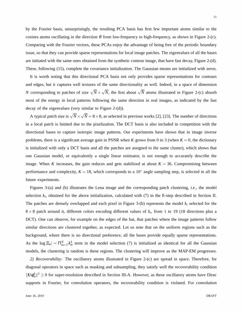
Figures 3-(a) and (b) illustrates the Lena image and the corresponding patch clustering, i.e., the model

selectionki, obtained for the above initialization, calculated with (7) in the E-step described in Section II.

The patches are densely overlapped and each pixel in Figure 3-(b) represents the modelki selected for the

8×8 patch around it, different colors encoding different values of ki, from 1 to 19 (18 directions plus a

DCT). One can observe, for example on the edges of the hat, that patches where the image patterns follow

similar directions are clustered together, as expected. Let us note that on the uniform regions such as the

background, where there is no directional preference, all the bases provide equally sparse representations.

As the log|Σk| = ΠNm=1λ k

m term in the model selection (7) is initialized as identical for all the Gaussian

models, the clustering is random is these regions. The clustering will improve as the MAP-EM progresses.

2) Recoverability:The oscillatory atoms illustrated in Figure 2-(c) are spread in space. Therefore, for

diagonal operators in space such as masking and subsampling, they satisfy well the recoverability condition

‖Uφ km‖2≥ 0 for super-resolution described in Section III-A. However, as these oscillatory atoms have Dirac

supports in Fourier, for convolution operators, the recoverability condition is violated. For convolution

June 16, 2010 DRAFT

12

(a) (b) (c) (d) (e)

Fig. 3. (a). Lena image. ((b) to (d) are color images.) (b). Patch clustering obtained with the initial directional PCAs(see Figure 2-(c)). The patches are densely overlapped and each pixel represents the modelki selected for the 8×8patch around it, different colors encoding different direction values ofki , from 1 to K = 19. (c). Patch clusteringobtained with the initial position PCAs (see Figure 4). Different colors encoding different position values ofki , from1 to P= 12. (d) and (e). Patch clustering with respectively directional and position PCAs after the 2nd iteration.

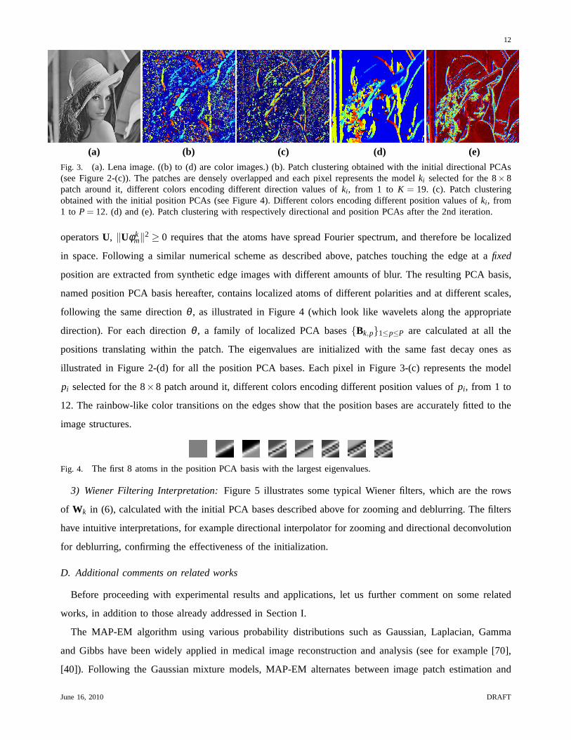
operatorsU, ‖Uφ km‖2 ≥ 0 requires that the atoms have spread Fourier spectrum, and therefore be localized

in space. Following a similar numerical scheme as describedabove, patches touching the edge at afixed

position are extracted from synthetic edge images with different amounts of blur. The resulting PCA basis,

named position PCA basis hereafter, contains localized atoms of different polarities and at different scales,

following the same directionθ , as illustrated in Figure 4 (which look like wavelets along the appropriate

direction). For each directionθ , a family of localized PCA basesBk,p1≤p≤P are calculated at all the

positions translating within the patch. The eigenvalues are initialized with the same fast decay ones as

illustrated in Figure 2-(d) for all the position PCA bases. Each pixel in Figure 3-(c) represents the model

pi selected for the 8×8 patch around it, different colors encoding different position values ofpi, from 1 to

12. The rainbow-like color transitions on the edges show that the position bases are accurately fitted to the

image structures.

Fig. 4. The first 8 atoms in the position PCA basis with the largest eigenvalues.

3) Wiener Filtering Interpretation:Figure 5 illustrates some typical Wiener filters, which are the rows

of Wk in (6), calculated with the initial PCA bases described above for zooming and deblurring. The filters

have intuitive interpretations, for example directional interpolator for zooming and directional deconvolution

for deblurring, confirming the effectiveness of the initialization.

D. Additional comments on related works

Before proceeding with experimental results and applications, let us further comment on some related

works, in addition to those already addressed in Section I.

The MAP-EM algorithm using various probability distributions such as Gaussian, Laplacian, Gamma

and Gibbs have been widely applied in medical image reconstruction and analysis (see for example [70],

[40]). Following the Gaussian mixture models, MAP-EM alternates between image patch estimation and

June 16, 2010 DRAFT

13

(a) (b) (c) (d)

Fig. 5. Some filters generated by the MAP estimator. (a) and (b) are for image zooming, where the degradation operatorU is a 2×2 subsampling operator. Gray-level from white to black: values from negative to positive. (a) is computedwith a Gaussian distribution whose PCA basis is a DCT basis, and it implements an isotropic interpolator. (b) iscomputed with a Gaussian distribution whose PCA basis is a directional PCA basis (angleθ = 30), and it implementsa directional interpolator. (c) and (d) are shown in Fourierand are for image deblurring, where the degradation operatorU is a Gaussian convolution operator. Gray-level from white to black: Fourier modules from zero to positive. (c) iscomputed with a Gaussian distribution whose PCA basis is a DCT basis, and it implements an isotropic deblurringfilter. (d) is computed with a Gaussian distribution whose PCA basis is a directional PCA basis (angleθ = 30, at afixed position), and it implements a directional deblurringfilter.

clustering, and Gaussian models estimation. Clustering-based estimation has been shown effective for image

restoration. To achieve accurate clustering-based estimation, an appropriate clustering is at the heart. In

a denoising setting where images are noisy but not degraded by the linear operatorU, clustering with

block matching, i.e., calculating Euclidian distance between image patch gray-levels [10], [17], [42], and

with image segmentation algorithms such as k-means on localimage features [15], have been shown to

improve the denoising results. For inverse problems where the observed images are degraded, for example

images with holes in an inpainting setting, clustering becomes more difficult. The generalized PCA [64]

models and segments data using an algebraic subspace clustering technique based on polynomial fitting and

differentiation, and while it has been shown effective in image segmentation, it does not reach state-of-the-

art in image restoration. In the recent non-parametric Bayesian approach [71], an image patch clustering is

implemented with probability models, which improves the denoising and inpainting results, although still

under performing, in quality and computational cost, the framework here introduced. The clustering in the

MAP-EM procedure enjoys the advantage of being completely consistent with the signal estimation, and in

consequence leads to state-of-the-art results in a number of imaging inverse problem applications.

IV. I NITIAL SUPPORTIVEEXPERIMENTS

Before proceeding with detailed experimental results for anumber of applications of the proposed frame-

work, this section shows through some basic experiments theeffectiveness and importance of the initialization

proposed above, the evolution of the representations as theMAP-EM algorithm iterates, as well as the

improvement brought by the structure in PLE with respect to traditional sparse estimation.

Following some recent works, e.g., [44], an image is decomposed into 128×128 regions, each region

treated with the MAP-EM algorithm separately. The idea is that image contents are often more coherent

semi-locally than globally, and Gaussian model estimationor dictionary learning can be slightly improved

in semi-local regions. This also saves memory and enables the processing to proceed as the image is being

transmitted. Parallel processing on image regions is also possible when the whole image is available. Regions

June 16, 2010 DRAFT

14

are half-overlapped to eliminate the boundary effect between the regions, and their estimates are averaged

at the end to obtain the final estimate.

A. Initialization

Different initializations are compared in the context of different inverse problems, inpainting, zooming

and deblurring. The reported experiments are performed on some typical image regions, Lena’s hat with

sharp contours and Barbara’s cloth rich in texture, as illustrated in Figure 6.

Inpainting. In the addressed case of inpainting, the image is degraded byU, that is a random masking

operator which randomly sets pixel values to zeros. The initialization described above is compared with a

random initialization, which initializes in the E-step allthe missing pixel value with zeros and starts with

a random patch clustering. Figure 6-(a) and (b) compare the PSNRs obtained by the MAP-EM algorithm

with those two initializations. The algorithm with the random initialization converges to a PSNR close to,

about 0.4 dB lower than, that with the proposed initialization, and the convergence takes much longer time

(about 6 iterations) than the latter (about 3 iterations).

It is worth noting that on the contours of Lena’s hat, with theproposed initialization the resulting PSNR

is stable from the initialization, which already produces accurate estimation, since the initial directional PCA

bases themselves are calculated over synthetic contour images, as described in Section III-C.

Zooming. In the context of zooming, the degradationU is a subsampling operator on a uniform grid, much

structured than that for inpainting. The MAP-EM algorithm with the random initialization completely fails

to work: It gets stuck in the initialization and does not leadto any changes on the degraded image. Instead

of initializing the missing pixels with zeros, a bicubic initialization is tested, which initializes the missing

pixels with bicubic interpolation. Figure 6-(c) shows that, as the MAP-EM algorithm iterates, it significantly

improves the PSNR over the bicubic initialization, however, the PSNR after a slower convergence is still

about 0.5 dB lower than that obtained with the proposed initialization.

Deblurring. In the deblurring setting, the degradationU is a convolution operator, which is very structured,

and the image is further contaminated with a white Gaussian noise. Four initializations are under considera-

tion: the initialization with directional PCAs (K directions plus a DCT basis), which is exactly the same as

that for inpainting and zooming tasks, the proposed initialization with thepositionPCA bases for deblurring

as described in Section III-C2 (P positions per each of theK directions, all with the same eigenvalues as for

the directional PCAs initialization), and two random initializations with the blurred image itself as the initial

estimate and a random patch clustering with, respectively,K +1 and (K +1)P clusters. As illustrated in

Figure 6-(d), the algorithm with the directional PCAs initialization gets stuck in a local minimum since the

second iteration, and converges to a PSNR 1.5 dB lower than that with the initialization using the position

June 16, 2010 DRAFT

15

PCAs. Indeed, since the recoverability condition for deblurring, as explained in Section III-C2, is violated

with just directional PCA bases, the resulting images remain still quite blurred. The random initialization

with (K +1)P clusters results in better results than withK +1 clusters, which is 0.7 dB worse than the

proposed initialization with position PCAs.

These experiments confirm the importance of the initialization in the MAP-EM algorithm to solve inverse

problems. The sparse coding dual interpretation of GMM/MAP-EM helps to deduce effective initializations

for different inverse problems. While for inpainting with random masking operators, trivial initializations

slowly converge to a solution moderately worse than that obtained with the proposed initialization, for more

structured degradation operators such as uniform subsampling and convolution, simple initializations either

completely fail to work or lead to significantly worse results than with the proposed initialization.

(a) (b) (c) (d)

Fig. 6. PSNR comparison of the MAP-EM algorithm with different initializations on different inverse problems. Thehorizontal axis corresponds to the number of iterations. (a) and (b). Inpainting with 50% and 30% available data, onLena’s hat and Barbara’s cloth. The initializations under consideration are the random initialization and the initializationwith directional PCA bases. (c) Zooming, on Lena’s hat. The initializations under consideration are bicubic initializationand the initialization with directional PCA bases. (Randominitialization completely fails to work.) (d) Deblurring,onLena’s hat. The initializations under consideration are the initialization with directional PCAs (K directions plus aDCT basis), the initialization with thepositionPCA bases (P positions per each of theK directions), and two randominitializations with the blurred image itself as the initial estimate and a random patch clustering with, respectively,K+1 (rand. 1) and(K +1)P (rand. 2) clusters. See text for more details.

B. Evolution of Representations

Figure 7 illustrates, in an inpainting context on Barbara’scloth, which is rich in texture, the evolution of the

patch clustering as well as that of a typical PCA bases as the MAP-EM algorithm iterates. The clustering gets

cleaned up as the algorithm iterates. (See figures 3-(d) and (e) for another example.) Some high-frequency

atoms are promoted to better capture the oscillatory patterns, resulting in a significant PSNR improvement

of more than 3 dB. On contour images such as Lena’s hat illustrated in Figure 6, on the contrary, although

the patch clustering is cleaned up as the algorithm iterates, the resulting local PSNR evolves little after the

initialization, which already produces accurate estimation, since the directional PCA bases themselves are

calculated over synthetic contour images, as described in Section III-C. The eigenvalues have always fast

decay as the iteration goes on, visually similar to the plot in Figure 2-(d). The resulting PSNRs typically

converge in 3 to 5 iterations.

June 16, 2010 DRAFT

16

(a) (b) (c) (d) (e)

Fig. 7. Evolution of the representations. (a) The original image cropped from Barbara. (b) The image masked with30% available data. (c) and (d) are color images. (c) Bottom:The first few atoms of an initial PCA basis correspondingto the texture on the right of the image. Top: The resulting patch clustering after the 1st iteration. Different colorsrepresent different clusters. (d) Bottom: The first few atoms of the PCA basis updated after the 1st iteration. Top: Theresulting patch clustering after the 2nd iteration. (e) Theinpainting estimate after the 2nd iteration (32.30 dB).

C. Estimation Methods

(a) Original image. (b) Low-resolution image. (c) Globall1: 22.70 dB (d) Global OMP: 28.24 dB

(e) Block l1: 26.35 dB (f) Block OMP: 29.27 dB (g) Block weighted l1: 35.94 dB (h) Block weightedl2: 36.45 dB

Fig. 8. Comparison of different estimation methods on super-resolution zooming. (a) The original image croppedfrom Lena. (b) The low-resolution image, shown at the same scale by pixel duplication. From (c) to (h) are thesuper-resolution results obtained with different estimation methods. See text for more details.

From the sparse coding point of view, the gain of introducingstructure in sparse inverse problem estimation

as described in Section III is now shown through some experiments. An overcomplete dictionaryD composed

of a family of PCA basesBk1≤k≤K, illustrated in Figure 1-(b), is learned as described in Section II, and

is then fed to the following estimation schemes. (i)Global l1 and OMP: the ensemble ofD is used as

an overcomplete dictionary, and the zooming estimation is calculated with the sparse estimate (13) through,

respectively, anl1 minimization or an orthogonal matching pursuit (OMP). (ii)Block l1 and OMP: the

sparse estimate is calculated in each PCA basisBk through, respectively anl1 minimization and an OMP,

and the best estimate is selected with a model selection procedure similar to (7), thereby reducing the degree

June 16, 2010 DRAFT

17

of freedom in the estimation with respect to the globall1 and OMP. [67]. (iii) Block weighted l1: on top

of the blockl1, weights are included for each coefficient amplitude in the regularizer,

aki = argmin

ai

(

‖UiBkai−yi‖2+σ2N

∑m=1

|ai[m]|τk

m

)

, (18)

with the weightsτkm = (λ k

m)1/2, whereλ k

m are the eigenvalues of thek-th PCA basis. The weighting scheme

penalizes the atoms that are less likely to be important, following the spirit of the weightedl2 deduced from

the MAP estimate. (iv)Block weighted l2: the proposed PLE. Comparing with (18), the difference is that

the weightedl2 (17) takes the place of the weightedl1, thereby transforming the problem into a stable and

computationally efficient piecewise linear estimation.

The comparison on a typical region of Lena in the 2×2 image zooming context is shown in Figure 8.

The globall1 and OMP produce some clear artifacts along the contours, which degrade the PSNRs. The

block l1 or OMP considerably improves the results (especially forl1). Comparing with the blockl1 or OMP,

a very significant improvement is achieved by adding the collaborative weights on top of the blockl1. The

proposed PLE with the block weightedl2, computed with linear filtering, further improves the estimation

accuracy over the block weightedl1, with a much lower computational cost.

In the following sections, PLE will be applied to a number of inverse problems, including image inpainting,

zooming and deblurring. The experiments are performed on some standard gray-level and color images,

illustrated in Figure 9.

Fig. 9. Images used in the numerical experiments. From top to bottom, left to right. The first eight are gray-level images:Lena (512× 512), Barbara (512× 512), Peppers (512×512), Mandril (512×512), House (256× 256), Cameraman(256× 256), Boats(512× 512), and Straws (640× 640). The rest are color images: Castle (481× 321), Mushroom(481×321), Kangaroo (321×481), Train (321×481), Horses (321×481), Kodak05 (512×768), Kodak20 (512×768),Girl (258×255), and Flower (171×330).

V. INPAINTING

In the addressed case of inpainting, the original imagef is masked with a random mask,y = Uf, whereU

is a diagonal matrix whose diagonal entries are randomly either 1 or 0, keeping or killing the corresponding

pixels. Note that this can be considered as a particular caseof compressed sensing, or when collectively

considering all the image patches, as matrix completion (and as here demonstrated, in contrast with the

recent literature on the subject, a single subspace is not sufficient, see also [71]).

June 16, 2010 DRAFT

18

The experiments are performed on the gray-level images Lena, Barbara, House, and Boat, and the color

images Castle, Mushroom, Train and Horses. Uniform random masks that retain 80%, 50%, 30% and 20%

of the pixels are used. The masked images are then inpainted with the algorithms under consideration.

For gray-level images, the image patch size is√

N×√

N = 8×8 when the available data is 80%, 50%,

and 30%. Larger patches of size 12×12 are used when images are heavily masked with only 20% pixels

available. For color images, patches of size√

N×√

N×3 throughout the RGB color channels are used to

exploit the redundancy among the channels [43]. To simplifythe initialization in color image processing,

the E-step in the first iteration is calculated with “gray-level” patches of size√

N×√

N on each channel, but

with a unified model selection across the channels: The same model selection is performed throughout the

channels by minimizing the sum of the model selection energy(7) over all the channels; the signal estimation

is calculated in each channel separately. The M-step then estimates the Gaussian models with the “color”

patches of size√

N×√

N×3 based on the model selection and the signal estimate previously obtained in

the E-step. Starting from the second iteration, both the E- and M-steps are calculated with “color” patches,

treating the√

N×√

N×3 patches as vectors of size 3N.√

N is set to 6 for color images, as in the previous

works [43], [71]. The MAP-EM algorithm runs for 5 iterations. The noise standard deviationσ is set to

3, which corresponds to the typical noise level in these images. The small constantε in the covariance

regularization is set to 30 in all the experiments.

The PLE inpainting is compared with a number of recent methods, including “MCA” (morphological

component analysis) [24], “ASR” (adaptive sparse reconstructions) [33] , “ECM” (expectation conditional

maximization) [27] , “KR” (kernel regression) [60], “FOE” (fields of experts) [56], “BP” (beta process) [71],

and “K-SVD” [43]. MCA and ECM compute the sparse inverse problem estimate in a dictionary that

combines a curvelet frame [11], a wavelet frame [45] and a local DCT basis. ASR calculates the sparse

estimate with a local DCT. BP infers a nonparametric Bayesian model from the image under test (noise

level is automatically estimated). Using a natural image training set, FOE and K-SVD learn respectively a

Markov random field model and an overcomplete dictionary that gives sparse representation for the images.

The results of MCA, ECM, KR, FOE are generated by the originalauthors’ softwares, with the parameters

manually optimized, and those of ASR are calculated with ourown implementation. The PSNRs of BP

and K-SVD are cited from the corresponding papers. K-SVD andBP currently generate the best inpainting

results in the literature.

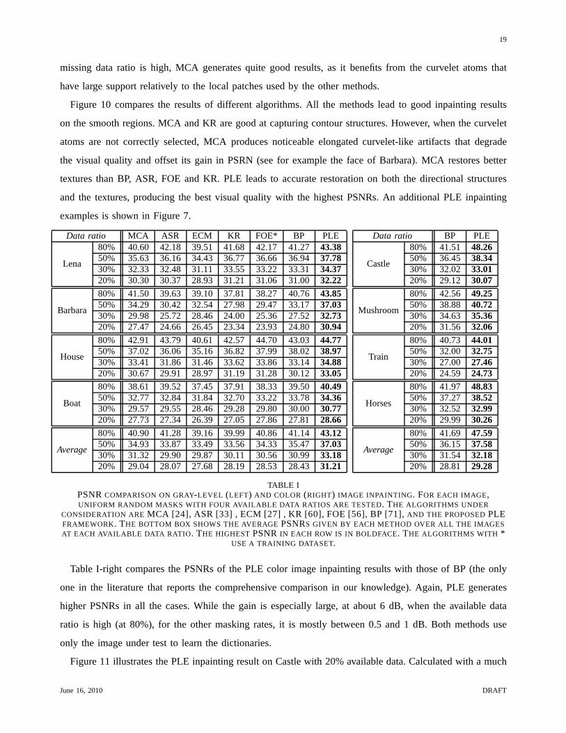
Table I-left gives the inpainting results on gray-level images. PLE considerably outperforms the other

methods in all the cases, with a PSNR improvement of about 2 dBon average over the second best algorithms

(BP, FOE and MCA). With 20% available data on Barbara, which is rich in textures, it gains as much as

about 3 dB over MCA, 4 dB over ECM and 6 dB over all the other methods. Let us remark that when the

June 16, 2010 DRAFT

19

missing data ratio is high, MCA generates quite good results, as it benefits from the curvelet atoms that

have large support relatively to the local patches used by the other methods.

Figure 10 compares the results of different algorithms. Allthe methods lead to good inpainting results

on the smooth regions. MCA and KR are good at capturing contour structures. However, when the curvelet

atoms are not correctly selected, MCA produces noticeable elongated curvelet-like artifacts that degrade

the visual quality and offset its gain in PSRN (see for example the face of Barbara). MCA restores better

textures than BP, ASR, FOE and KR. PLE leads to accurate restoration on both the directional structures

and the textures, producing the best visual quality with thehighest PSNRs. An additional PLE inpainting

examples is shown in Figure 7.

Data ratio MCA ASR ECM KR FOE* BP PLE

Lena

80% 40.60 42.18 39.51 41.68 42.17 41.27 43.3850% 35.63 36.16 34.43 36.77 36.66 36.94 37.7830% 32.33 32.48 31.11 33.55 33.22 33.31 34.3720% 30.30 30.37 28.93 31.21 31.06 31.00 32.22

Barbara

80% 41.50 39.63 39.10 37.81 38.27 40.76 43.8550% 34.29 30.42 32.54 27.98 29.47 33.17 37.0330% 29.98 25.72 28.46 24.00 25.36 27.52 32.7320% 27.47 24.66 26.45 23.34 23.93 24.80 30.94

House

80% 42.91 43.79 40.61 42.57 44.70 43.03 44.7750% 37.02 36.06 35.16 36.82 37.99 38.02 38.9730% 33.41 31.86 31.46 33.62 33.86 33.14 34.8820% 30.67 29.91 28.97 31.19 31.28 30.12 33.05

Boat

80% 38.61 39.52 37.45 37.91 38.33 39.50 40.4950% 32.77 32.84 31.84 32.70 33.22 33.78 34.3630% 29.57 29.55 28.46 29.28 29.80 30.00 30.7720% 27.73 27.34 26.39 27.05 27.86 27.81 28.66

Average

80% 40.90 41.28 39.16 39.99 40.86 41.14 43.1250% 34.93 33.87 33.49 33.56 34.33 35.47 37.0330% 31.32 29.90 29.87 30.11 30.56 30.99 33.1820% 29.04 28.07 27.68 28.19 28.53 28.43 31.21

Data ratio BP PLE

Castle

80% 41.51 48.2650% 36.45 38.3430% 32.02 33.0120% 29.12 30.07

Mushroom

80% 42.56 49.2550% 38.88 40.7230% 34.63 35.3620% 31.56 32.06

Train

80% 40.73 44.0150% 32.00 32.7530% 27.00 27.4620% 24.59 24.73

Horses

80% 41.97 48.8350% 37.27 38.5230% 32.52 32.9920% 29.99 30.26

Average

80% 41.69 47.5950% 36.15 37.5830% 31.54 32.1820% 28.81 29.28

TABLE IPSNRCOMPARISON ON GRAY-LEVEL (LEFT) AND COLOR (RIGHT) IMAGE INPAINTING . FOR EACH IMAGE,UNIFORM RANDOM MASKS WITH FOUR AVAILABLE DATA RATIOS ARE TESTED. THE ALGORITHMS UNDER

CONSIDERATION AREMCA [24], ASR [33] , ECM [27] , KR [60], FOE [56], BP [71],AND THE PROPOSEDPLEFRAMEWORK. THE BOTTOM BOX SHOWS THE AVERAGEPSNRS GIVEN BY EACH METHOD OVER ALL THE IMAGESAT EACH AVAILABLE DATA RATIO . THE HIGHEST PSNRIN EACH ROW IS IN BOLDFACE. THE ALGORITHMS WITH *

USE A TRAINING DATASET.

Table I-right compares the PSNRs of the PLE color image inpainting results with those of BP (the only

one in the literature that reports the comprehensive comparison in our knowledge). Again, PLE generates

higher PSNRs in all the cases. While the gain is especially large, at about 6 dB, when the available data

ratio is high (at 80%), for the other masking rates, it is mostly between 0.5 and 1 dB. Both methods use

only the image under test to learn the dictionaries.

Figure 11 illustrates the PLE inpainting result on Castle with 20% available data. Calculated with a much

June 16, 2010 DRAFT

20

(a) Original (b) Masked (c) MCA (24.18 dB) (d) ASR (21.84 dB)

(e) KR (21.55 dB) (f) FOE (21.92 dB) (g) BP (25.54 dB) (h) PLE (27.65 dB)

Fig. 10. Gray-level image inpainting. (a) Original image cropped from Barbara. (b) Masked image with 20% availabledata (6.81 dB). From (c) to (g): Image inpainted by differentalgorithms. Note the overall superior visual qualityobtained with the proposed approach. The PSNRs are calculated on the cropped images.

reduced computational complexity, the resulting 30.07 dB PSNR surpasses the highest PSNR, 29.65 dB,

reported in the literature, produced by K-SVD [43], that uses a dictionary learned from a natural image

training set, followed by 29.12 dB given by BP (BP has been recently improved adding spatial coherence

in the code, unpublished results). As shown in the zoomed region, PLE accurately restores the details of the

castle from the heavily masked image. Let us remark that inpainting with random masks on color images is

in general more favorable than on gray-level images, thanksto the information redundancy among the color

channels.

(a) Original (b) Masked (c) PLE

Fig. 11. Color image inpainting. (a) Original image cropped from Castle. (b) Masked image with 20% available data(5.44 dB). (c) Image inpainted by PLE (27.30 dB). The PSNR on the overall image obtained with PLE is 30.07 dB,higher than the best result reported so far in the literature29.65 dB [43].

VI. I NTERPOLATION ZOOMING

Interpolation zooming is a special case of inpainting with regular subsampling on uniform grids. As

explained in Section III-A, the regular subsampling operator U may result in a highly coherent transformed

June 16, 2010 DRAFT

21

dictionaryUD. Calculating an accurate sparse estimation for interpolation zooming is therefore more difficult

than that for inpainting with random masks.

The experiments are performed on the gray-level images Lena, Peppers, Mandril, Cameraman, Boat, and

Straws, and the color images Lena, Peppers, Kodak05 and Kokad20. The color images are treated in the

same way as for inpainting. These high-resolution images are down-sampled by a factor 2× 2 without

anti-aliasing filtering. The resulting low-resolution images are aliased, which corresponds to the reality of

television images that are usually aliased, since this improves their visual perception. The low-resolution

images are then zoomed by the algorithms under consideration. When the anti-aliasing blurring operator is

included before subsampling, zooming can be casted as a deconvolution problem and will be addressed in

Section VII.

The PLE interpolation zooming is compared with linear interpolators [8], [37], [63], [52] as well as recent

super-resolution algorithms “NEDI” (new edge directed interpolation) [39], “DFDF” (directional filtering

and data fusion) [68], “KR” (kernel regression) [60], “ECM”(expectation conditional maximization) [27],

“Contourlet” [51], “ASR” (adaptive sparse reconstructions) [33], “FOE” (fields of experts) [56], “SR”

(sparse representation) [65], “SAI” (soft-decision adaptive Interpolation) [69] and “SME” (sparse mixing

estimators) [47]. KR, ECM, ASR and FOE are generic inpainting algorithms that have been described in

Section V. NEDI, DFDF and SAI are adaptive directional interpolation methods that take advantage of the

image directional regularity. Contourlet is a sparse inverse problem estimator as described in Section III-A,

computed in a contourlet frame. SR is also a sparse inverse estimator that learns the dictionaries from

a training image set. SME is a recent zooming algorithm that exploits directional structured sparsity in

wavelet representations. Among the previously published algorithms, SAI and SME currently provide the

best PSNR for spatial image interpolation zooming [47], [69]. The results of ASR are generated with our own

implementation, and those of all the other algorithms are produced by the original authors’ softwares, with

the parameters manually optimized. As the anti-aliasing operator is not included in the interpolation zooming

model, to obtain correct results with SR, the anti-aliasingfilter used in the original authors’ SR software is

deactivated in both dictionary training (with the authors’original training dataset of 92 images) and super-

resolution estimation. PLE is configured in the same way as for inpainting as described in Section V, with

patch size 8×8 for gray-level images, and 6×6×3 for color images.

Table II gives the PSNRs generated by all algorithms on the gray-level and the color images. Bicubic

interpolation provides nearly the best results among all tested linear interpolators, including cubic splines [63],

MOMS [8] and others [52], due to the aliasing produced by the down-sampling. PLE gives moderately higher

PSNRs than SME and SAI for all the images, with one exception where the SAI produces slightly higher

PSNR. Their gain in PSNR is significantly larger than with allthe other algorithms.

June 16, 2010 DRAFT

22

Figure 12 compares an interpolated image obtained by the baseline bicubic interpolation and the algorithms

that generate the highest PSNRs, SAI and PLE. The local PSNRson the cropped images produced by all

the methods under consideration are reported as well. Bicubic interpolation produces some blur and jaggy

artifacts in the zoomed images. These artifacts are reducedto some extent by the NEDI, DFDF, KR and FOE

algorithms, but the image quality is still lower than with PLE, SAI and SME algorithms, as also reflected in

the PSNRs. SR yields an image that looks sharp. However, due to the coherence of the transformed dictionary,

as explained in Section III-A, when the approximating atomsare not correctly selected, it produces artifact

patterns along the contours, which degrade its PSNR. The PLEalgorithm restores slightly better than SAI

and SME on regular geometrical structures, as can be observed on the upper and lower propellers, as well

as on the fine lines on the side of the plane indicated by the arrows.

Bicubic NEDI DFDF KR ECM Contourlet ASR FOE* SAI SME PLELena 33.93 33.77 33.91 33.94 24.31 33.92 33.19 34.04 34.68 34.58 34.76

Peppers 32.83 33.00 33.18 33.15 23.60 33.10 32.33 31.90 33.52 33.52 33.62Mandril 22.92 23.16 22.83 22.93 20.34 22.53 22.66 22.99 23.19 23.16 23.27

Cameraman 25.37 25.42 25.67 25.51 19.50 25.35 25.33 25.58 25.88 26.26 26.47Boat 29.24 29.19 29.32 29.18 22.20 29.25 28.96 29.36 29.68 29.76 29.93

Straws 20.53 20.54 20.70 20.76 17.09 20.52 20.54 20.47 21.48 21.61 21.82Ave. gain 0 0.04 0.13 0.11 -6.30 -0.02 -0.30 -0.08 0.60 0.68 0.84

Bicubic NEDI DFDF KR FOE* SR* SAI SME PLELena 32.41 32.47 32.46 32.55 32.55 26.42 32.98 32.88 33.53

Peppers 30.95 31.06 31.24 31.26 31.05 26.43 31.37 31.35 31.88Kodak05 25.82 25.93 26.03 26.09 26.01 20.76 26.91 26.72 26.77Kodak20 30.65 31.06 31.08 30.97 30.84 25.92 31.51 31.38 31.72Ave. gain 0 0.17 0.25 0.27 0.16 -5.07 0.74 0.63 1.02

TABLE IIPSNRCOMPARISON ON GRAY-LEVEL (TOP) AND COLOR (BOTTOM) IMAGE INTERPOLATION ZOOMING. THE

ALGORITHMS UNDER CONSIDERATION ARE BICUBIC INTERPOLATION, NEDI [39], DFDF [68], KR [60],ECM [27], CONTOURLET [51], ASR [33], FOE [56], SR [65], SAI [69] , SME [47]AND THE PROPOSEDPLE

FRAMEWORK. THE BOTTOM ROW SHOWS THE AVERAGE GAIN OF EACH METHOD RELATIVE TO THE BICUBICINTERPOLATION. THE HIGHESTPSNRIN EACH ROW IS IN BOLDFACE. THE ALGORITHMS WITH * USE A TRAINING

DATASET.

VII. D EBLURRING

An imagef is blurred and contaminated by additive noise,y = Uf+w, whereU is a convolution operator

andw is the noise. Image deblurring aims at estimatingf from the blurred and noisy observationy.

A. Hierarchical PLE

As explained in Section III-C2, the recoverability condition of sparse super-resolution estimates for

deblurring requires a dictionary comprising atoms with spread Fourier spectrum and thus localized in space,

such as the position PCA basis illustrated in Figure 4. To reduce the computational complexity, model

selection with a hierarchy of directional PCA bases and position PCA bases is proposed, in the same spirit

June 16, 2010 DRAFT

23

(a) HR (b) LR (c) Bibubic (d) SAI (e) PLE

Fig. 12. Color image zooming. (a) Crop from the high-resolution image Kodak20. (b) Low-resolution image. From (c)to (e), images zoomed by bicubic interpolation (28.48 dB), SAI (30.32 dB) [69], and proposed PLE framework (30.64dB). PSNRs obtained by the other methods under consideration: NEDI (29.68 dB) [39], DFDF (29.41 dB) [68], KR(29.49 dB) [60], FOE (28.73 dB) [56], SR (23.85 dB) [65], and SME (29.90 dB) [47]. Attention should be focusedon the places indicated by the arrows.

of [66]. Figure 13-(a) illustrates the hierarchical PLE with a cascade of the two layers of model selections.

The first layer selects the direction, and given the direction, the second layer further specifies the position.

In the first layer, the model selection procedure is identical to that in image inpainting and zooming, i.e., it

is calculated with the Gaussian models corresponding to thedirectional PCA basesBk1≤k≤K, Figure 2-(c).

In this layer, a directional PCABk of orientationθ is selected for each patch. Given the directional basisBk

selected in the first layer, the second layer recalculates the model selection (7), this time with a family of

position PCA basesBk,p1≤p≤P corresponding to the same directionθ as the directional basisBk selected

in the first layer, with atoms in each basisBk,p localized at one position, and theP bases translating in

space and covering the whole patch. The image patch estimation (8) is obtained in the second layer. This

hierarchical calculation reduces the computational complexity from O(KP) to O(K +P).

(a) (b)

Fig. 13. (a). Hierarchical PLE for deblurring. Each patch in the firstlayer symbolizes a directional PCA basis. Eachpatch in the second layer symbolizes a position PCA basis. (b) To circumvent boundary issues, deblurring a patchwhose support isΩ can be casted as inverting an operator compounded by a masking and a convolution defined on alarger supportΩ. See text for details.

For deblurring, boundary issues on the patches need to be addressed. Since the convolution operator is non-

diagonal, the deconvolution of each pixely(x) in the blurred imagey involves the pixels in a neighborhood

aroundx whose size depends on the blurring kernel. As the patch basedmethods deal with the local patches,

for a given patch, the information outside of it is missing. Therefore, it is impossible to obtain accurate

June 16, 2010 DRAFT

24

deconvolution estimation on the boundaries of the patches.To circumvent this boundary problem, a larger

patch is considered and the deconvolution is casted as a deconvolution plus an inpainting problem. Let us

retake the notationsf i , yi andwi to denote respectively the patches of size√

N×√

N in the original image

f, the degraded imagey, and the noisew. Let Ω be their support. Letf i , yi and wi be the corresponding

larger patches of size(√

N+2r)× (√

N+2r), whose supportΩ is centered at the same position asΩ and

with an extended boundaryΩ\Ω of width r (the width of the blurring kernel, see below), as illustrated in

Figure 13-(b). LetU be an extension of the convolution operatorU on Ω such thatUf i(x) = Uf i(x) if x∈Ω,

and 0 if x∈ Ω\Ω. Let M be a masking operator defined onΩ which keeps all the pixels in the central part

Ω and kills the rest, i.e.,Mf i(x) = f i(x) if x∈Ω, and 0 if x∈ Ω\Ω. If the width r of the boundaryΩ\Ω is

larger than the radius of the blurring kernel, one can show that the blurring operation can be rewritten locally

as an extended convolution on the larger support followed bya masking,Myi = MUf i +Mwi . Estimatingf i

from yi can thus be calculated by estimatingf i from Myi , following exactly the same algorithm, now treating

the compoundedMU as the degradation operator to be inverted. The boundary pixels in the estimatef i(x),

x∈ Ω\Ω, can be interpreted as an extrapolation fromyi , therefore less reliable. The deblurring estimatef i

is obtained by discarding these boundary pixels from˜f i (which are outside ofΩ anyway).

Local patch based deconvolution algorithms become less accurate if the blurring kernel support is large

relative to the patch size. In the deconvolution experiments reported below,Ω andΩ are respectively set to

8×8 and 12×12. The blurring kernels are restricted to a 5×5 support.

B. Deblurring Experiments

The deblurring experiments are performed on the gray-levelimages Lena, Barbara, Boat, House, and

Cameraman, with different amounts of blur and noise. The PLEdeblurring is compared with a number

of deconvolution algorithms: “ForWaRD” (Fourier-waveletregularized deconvolution) [53], “TVB” (total

variation based) [7], “TwIST” (two-step iterative shrinkage/thresholding) [6], “SP” (sparse prior) [38], “SA-

DCT” (shape adaptive DCT) [28], “BM3D” (3D transform-domain collaborative filtering) [18], and “DSD”

(direction sparse deconvolution) [41]. ForWaRD, SA-DCT and BM3D first calculate the deconvolution with

a regularized Wiener filter in Fourier, and then denoise the Wiener estimate with, respectively, a thresholding

estimator in wavelet and SA-DCT representations, and with the non-local 3D collaborative filtering [17].

TVB and TwIST deconvolutions regularize the estimate with the image total variation prior. SP assumes a

sparse prior on the image gradient. DSD is a recently developed sparse inverse problem estimator, described

in Section III-A. In the previous published works, BM3D and SA-DCT are among the deblurring methods

that produce the highest PSNRs, followed by SP. The results of TVB, TwIST, SP, SA-DCT and DSD are

generated by the authors’ original softwares, with the parameters manually optimized, and those of ForWaRD

June 16, 2010 DRAFT

25

are calculated with our own implementation. The proposed algorithm runs for 5 iterations.

Table III gives the ISNRs (improvement in PSNR relative to the input image) of the different algorithms

for restoring images blurred with Gaussian kernels of standard deviationσb = 1 and 2 (truncated to a 5×5

support), and contaminated by a white Gaussian noise of standard deviationσn = 5. BM3D produces the

highest ISNRs, followed closely by SA-DCT and PLE, whose ISNRs are comparable and are moderately

higher than with SP on average. Let us remark that BM3D and SA-DCT apply an empirical Wiener filtering

as a post-processing that boosts the ISNR by near 1 dB. The empirical Wiener technique can be plugged

into other sparse transform-based methods such as PLE and ForWaRD as well. Without this post-processing,

PLE outperforms BM3D and SA-DCT on average.

Figure 14 shows a deblurring example. All the algorithms under consideration reduce the amount of

blur and attenuate the noise. BM3D generates the highest ISNR, followed by SA-DCT, PLE and SP, all

producing similar visual quality, which are moderately better than the other methods. DSD accurately restores

sharp image structures when the atoms are correctly selected, however, some artifacts due to the incorrect

atom selection offset its gain in ISNR. The empirical Wienerfiltering post-processing in BM3D and SA-

DCT efficiently removes some artifacts and significantly improves the visual quality and the ISNR. More

examples of PLE deblurring will be shown in the next section.

Kernel size and input PSNR ForWaRD TVB TwIST SA-DCT BM3D SP DSD* PLE

Lenaσb = 1 30.62 2.51 3.03 2.87 3.56/2.58 4.03/3.45 3.31 2.56 3.77σb = 2 28.84 2.33 3.15 3.13 3.46/3.00 3.91/3.20 3.40 2.47 3.52

Houseσb = 1 30.04 2.31 3.12 3.23 4.14/3.07 4.29/3.80 3.52 2.27 4.38σb = 2 28.02 2.29 3.24 3.82 4.21/3.64 4.73/4.11 3.92 2.97 3.90

Boatσb = 1 28.29 1.69 2.45 2.44 2.93/2.21 3.23/2.46 2.70 1.93 2.72σb = 2 26.21 1.63 2.67 2.59 3.71/2.63 3.33/2.44 2.60 2.02 2.48

Averageσb = 1 29.65 2.17 2.87 2.84 3.54/2.62 3.85/3.23 3.17 2.25 3.62σb = 2 27.69 2.08 3.02 3.18 3.79/3.09 3.99/3.25 3.30 2.48 3.31

TABLE IIIISNR (IMPROVEMENT IN PSNRWITH RESPECT TO INPUT IMAGE) COMPARISON ON IMAGE DEBLURRING. IMAGESARE BLURRED BY A GAUSSIAN KERNEL OF STANDARD DEVIATION σb = 1 AND 2, AND ARE THEN CONTAMINATEDBY WHITE GAUSSIAN NOISE OF STANDARD DEVIATIONσn = 5. FROM LEFT TO RIGHT: FORWARD [53], TVB [7],

TWIST [6], SA-DCT (WITH /WITHOUT EMPIRICAL WIENER POST-PROCESSING) [28], BM3D (WITH /WITHOUTEMPIRICAL WIENER POST-PROCESSING) [18], SP [38], DSD [41],AND THE PROPOSEDPLE FRAMEWORK. THEBOTTOM BOX SHOWS THE AVERAGEISNRS GIVEN BY EACH METHOD OVER ALL THE IMAGES WITH DIFFERENT

AMOUNTS OF BLUR. THE HIGHEST ISNR IN EACH ROW IS IN BOLDFACE, WHILE THE HIGHEST WITHOUTPOST-PROCESSING IS IN ITALIC. THE ALGORITHMS WITH * USE A TRAINING DATASET.

C. Zooming deblurring

When an anti-aliasing filtering is taken into account, imagezooming-out can be formulated asy = SUf,

wheref is the high-resolution image,U andS are respectively an anti-aliasing convolution and a subsampling

operator, andy is the resulting low-resolution image. Image zooming aims at estimatingf from y, which

amounts to inverting the combination of the two operatorsS andU.

June 16, 2010 DRAFT

26

(a) Original (b) Blurred and noisy (c) BM3D (D) PLE

Fig. 14. Gray-level image deblurring. (a) Crop from Lena. (b) Image blurred by a Gaussian kernel of standard deviationσb = 1 and contaminated by white Gaussian noise of standard deviation σn = 5 (PSNR=27.10). (c) and (d). Imagesdeblurred by BM3D with empirical Wiener post-processing (ISNR 3.40 dB dB) [18], and the proposed PLE framework(ISNR 2.94 dB). ISNR produced by the other methods under consideration: BM3D without empirical Wiener post-processing (2.65 dB) [18], TVB (2.72 dB) [7], TwIST (2.61dB)[6], SP (2.93 dB) [38], SA-DCT with/without empiricalWiener post-processing (2.95/2.10 dB) [28], and DSD (1.95 dB) [41].

Image zooming can be calculated differently under different amounts of blur introduced byU. Let us

distinguish between three cases: (i) If the anti-aliasing filtering U removes enough high-frequencies fromf

so thaty = SUf is free of aliasing, then the subsampling operatorS can be perfectly inverted with a linear

interpolation denoted asI , i.e., IS = Id [45]. In this case, zooming can can be calculated as a deconvolution

problem onIy = Uf, where one seeks to invert the convolution operatorU. In reality, however, camera and

television images contain, always a certain amount of aliasing, since it improves the visual perception, i.e.,

the anti-aliasing filteringU does not eliminate all the high-frequencies fromf. (ii) When U removes a small

amount of high-frequencies, which is often the case in reality, zooming can be casted as an interpolation

problem [39], [47], [51], [60], [68], [69], where one seeks to invert only S, as addressed in Section VI.

(iii) When U removes an intermediate amount of blur fromf, the optimal zooming solution is invertingSU

together as a compounded operator, as investigated in [65].

This section introduces a possible solution for the case (iii) with the PLE deblurring. A linear interpolation

I is first applied to partially invert the subsampling operator S. Due to the aliasing, the linear interpolation

does not perfectly restoreUf, nevertheless it remains rather accurate, i.e., the interpolated imageIy = ISUf

is close to the blurred imageUf, asUf has limited high-frequencies in the case (iii). The PLE deblurring

framework is then applied to deconvolveU from Iy . Inverting the operatorU is simpler than inverting the

compounded operatorSU. As the linear interpolationI in the first step is accurate enough in the case (iii),

deconvolvingIy results in accurate zooming estimates.

In the experiments below, the anti-aliasing filterU is set as a Gaussian convolution of standard deviation

σG = 1.0 and S is an s× s= 2× 2 subsampling operator. It has been shown that a pre-filtering with a

Gaussian kernel ofσG = 0.8s guarantees that the followings×s subsampling generates a quasi aliasing-free

image [50]. For a 2× 2 subsampling, the anti-aliasing filteringU with σG = 1.0 leads to an amount of

aliasing and visual quality similar to that in common camerapictures in reality.

Figure 15 illustrates an experiment on the image Lena. Figures 15-(a) to (c) show, respectively, a crop of

June 16, 2010 DRAFT

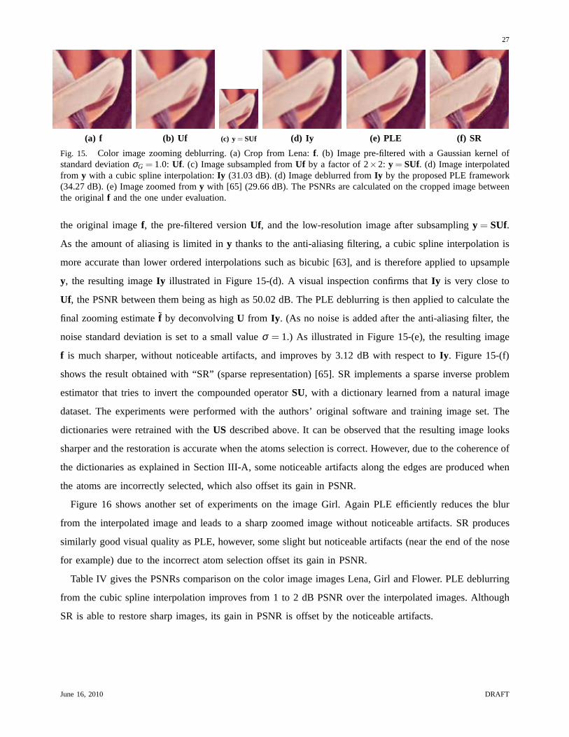
27

(a) f (b) Uf (c) y= SUf (d) Iy (e) PLE (f) SR

Fig. 15. Color image zooming deblurring. (a) Crop from Lena:f. (b) Image pre-filtered with a Gaussian kernel ofstandard deviationσG = 1.0: Uf. (c) Image subsampled fromUf by a factor of 2×2: y = SUf. (d) Image interpolatedfrom y with a cubic spline interpolation:Iy (31.03 dB). (d) Image deblurred fromIy by the proposed PLE framework(34.27 dB). (e) Image zoomed fromy with [65] (29.66 dB). The PSNRs are calculated on the croppedimage betweenthe originalf and the one under evaluation.

the original imagef, the pre-filtered versionUf, and the low-resolution image after subsamplingy = SUf.

As the amount of aliasing is limited iny thanks to the anti-aliasing filtering, a cubic spline interpolation is

more accurate than lower ordered interpolations such as bicubic [63], and is therefore applied to upsample

y, the resulting imageIy illustrated in Figure 15-(d). A visual inspection confirms that Iy is very close to

Uf, the PSNR between them being as high as 50.02 dB. The PLE deblurring is then applied to calculate the

final zooming estimatef by deconvolvingU from Iy . (As no noise is added after the anti-aliasing filter, the

noise standard deviation is set to a small valueσ = 1.) As illustrated in Figure 15-(e), the resulting image

f is much sharper, without noticeable artifacts, and improves by 3.12 dB with respect toIy . Figure 15-(f)

shows the result obtained with “SR” (sparse representation) [65]. SR implements a sparse inverse problem

estimator that tries to invert the compounded operatorSU, with a dictionary learned from a natural image

dataset. The experiments were performed with the authors’ original software and training image set. The

dictionaries were retrained with theUS described above. It can be observed that the resulting imagelooks

sharper and the restoration is accurate when the atoms selection is correct. However, due to the coherence of

the dictionaries as explained in Section III-A, some noticeable artifacts along the edges are produced when

the atoms are incorrectly selected, which also offset its gain in PSNR.

Figure 16 shows another set of experiments on the image Girl.Again PLE efficiently reduces the blur

from the interpolated image and leads to a sharp zoomed imagewithout noticeable artifacts. SR produces

similarly good visual quality as PLE, however, some slight but noticeable artifacts (near the end of the nose

for example) due to the incorrect atom selection offset its gain in PSNR.

Table IV gives the PSNRs comparison on the color image imagesLena, Girl and Flower. PLE deblurring

from the cubic spline interpolation improves from 1 to 2 dB PSNR over the interpolated images. Although

SR is able to restore sharp images, its gain in PSNR is offset by the noticeable artifacts.

June 16, 2010 DRAFT

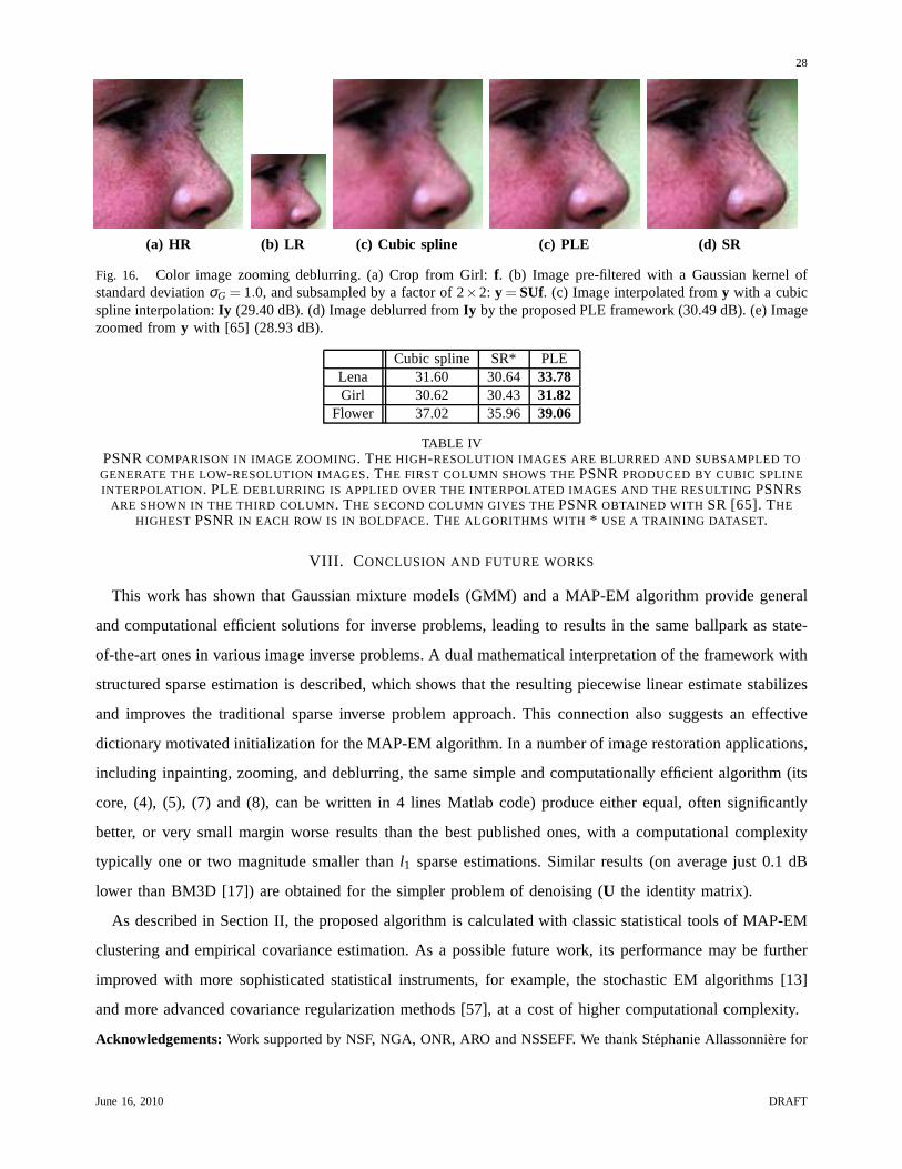
28

(a) HR (b) LR (c) Cubic spline (c) PLE (d) SR

Fig. 16. Color image zooming deblurring. (a) Crop from Girl:f. (b) Image pre-filtered with a Gaussian kernel ofstandard deviationσG = 1.0, and subsampled by a factor of 2×2: y = SUf. (c) Image interpolated fromy with a cubicspline interpolation:Iy (29.40 dB). (d) Image deblurred fromIy by the proposed PLE framework (30.49 dB). (e) Imagezoomed fromy with [65] (28.93 dB).

Cubic spline SR* PLELena 31.60 30.64 33.78Girl 30.62 30.43 31.82

Flower 37.02 35.96 39.06

TABLE IVPSNRCOMPARISON IN IMAGE ZOOMING. THE HIGH-RESOLUTION IMAGES ARE BLURRED AND SUBSAMPLED TOGENERATE THE LOW-RESOLUTION IMAGES. THE FIRST COLUMN SHOWS THEPSNRPRODUCED BY CUBIC SPLINEINTERPOLATION. PLE DEBLURRING IS APPLIED OVER THE INTERPOLATED IMAGES AND THE RESULTING PSNRS

ARE SHOWN IN THE THIRD COLUMN. THE SECOND COLUMN GIVES THEPSNROBTAINED WITH SR [65]. THEHIGHEST PSNRIN EACH ROW IS IN BOLDFACE. THE ALGORITHMS WITH * USE A TRAINING DATASET.

VIII. C ONCLUSION AND FUTURE WORKS

This work has shown that Gaussian mixture models (GMM) and a MAP-EM algorithm provide general

and computational efficient solutions for inverse problems, leading to results in the same ballpark as state-

of-the-art ones in various image inverse problems. A dual mathematical interpretation of the framework with

structured sparse estimation is described, which shows that the resulting piecewise linear estimate stabilizes

and improves the traditional sparse inverse problem approach. This connection also suggests an effective

dictionary motivated initialization for the MAP-EM algorithm. In a number of image restoration applications,

including inpainting, zooming, and deblurring, the same simple and computationally efficient algorithm (its

core, (4), (5), (7) and (8), can be written in 4 lines Matlab code) produce either equal, often significantly

better, or very small margin worse results than the best published ones, with a computational complexity

typically one or two magnitude smaller thanl1 sparse estimations. Similar results (on average just 0.1 dB

lower than BM3D [17]) are obtained for the simpler problem ofdenoising (U the identity matrix).

As described in Section II, the proposed algorithm is calculated with classic statistical tools of MAP-EM

clustering and empirical covariance estimation. As a possible future work, its performance may be further

improved with more sophisticated statistical instruments, for example, the stochastic EM algorithms [13]

and more advanced covariance regularization methods [57],at a cost of higher computational complexity.

Acknowledgements:Work supported by NSF, NGA, ONR, ARO and NSSEFF. We thank Stephanie Allassonniere for

June 16, 2010 DRAFT

29

helpful discussions, in particular about MAP-EM and covariance regularization.

REFERENCES

[1] J. Abernethy, F. Bach, T. Evgeniou, and J.P. Vert. A new approach to collaborative filtering: Operator estimation with spectralregularization.The Journal of Machine Learning Research, 10:803–826, 2009.

[2] M. Aharon, M. Elad, and A. Bruckstein. K-SVD: An algorithm for designing overcomplete dictionaries for sparse representation.IEEE Trans. on Signal Proc., 54(11):4311, 2006.

[3] S. Allassonniere, Y. Amit, and A. Trouve. Towards a coherent statistical framework for dense deformable template estimation.J.R. Statist. Soc. B, 69(1):3–29, 2007.

[4] R.G. Baraniuk, V. Cevher, M.F. Duarte, and C. Hegde. Model-based compressive sensing.Preprint, 2008.[5] J.P. Baudry, A.E. Raftery, G. Celeux, K. Lo, and R. Gottardo. Combining mixture components for clustering.Accepted to

Journal of Computational and Graphical Statistics, 2010.[6] J.M. Bioucas-Dias and M.A.T. Figueiredo. A new TwIST: two-step iterative shrinkage/thresholding algorithms for image

restoration.IEEE Trans. on Image Proc., 16(12):2992–3004, 2007.[7] J.M. Bioucas-Dias, M.A.T. Figueiredo, and J.P. Oliveira. Total variation-based image deconvolution: a majorization-

minimization approach. InICASSP, volume 2, 2006.[8] T. Blu, P. Thevenaz, and M. Unser. MOMS: Maximal-order interpolation of minimal support.IEEE Trans. on Image Proc.,

10(7):1069–1080, 2001.[9] S.P. Boyd and L. Vandenberghe.Convex Optimization. Cambridge University Press, 2004.

[10] A. Buades, B. Coll, and J.M. Morel. A review of image denoising algorithms, with a new one.Multiscale Modeling andSimulation, 4(2):490–530, 2006.

[11] E.J. Candes and D.L. Donoho. New tight frames of curvelets and optimal representations of objects with C2 singularities.Comm. Pure Appl. Math, 56:219–266, 2004.

[12] E.J. Candes and T. Tao. Near-optimal signal recovery from random projections: Universal encoding strategies?IEEE Trans.on Info. Theo., 52(12):5406–5425, 2006.

[13] G. Celeux and G. Govaert. A classification EM algorithm for clustering and two stochastic versions.Computational Statisticsand Data Analysis, 14(3):315–332, 1992.

[14] G. Celeux and G. Govaert. Gaussian parsimonious clustering models.Pattern Recognition, 28(5):781–793, 1995.[15] P. Chatterjee and P. Milanfar. Clustering-based denoising with locally learned dictionaries.IEEE Trans. on Image Proc., 18(7),

2009.[16] S.S. Chen, D.L. Donoho, and M.A. Saunders. Atomic decomposition by basis pursuit.SIAM J. on Sci. Comp., 20:33, 1999.[17] K. Dabov, A. Foi, V. Katkovnik, and K. Egiazarian. Imagedenoising by sparse 3-D transform-domain collaborative filtering.

IEEE Trans. on Image Proc., 16(8):2080–2095, 2007.[18] K. Dabov, A. Foi, V. Katkovnik, and K. Egiazarian. Imagerestoration by sparse 3D transform-domain collaborative filtering.

In SPIE Electronic Imaging, 2008.[19] I. Daubechies, M. Defrise, and C. De Mol. An iterative thresholding algorithm for linear inverse problems with a sparsity

constraint.Comm. Pure Appl. Math, 57:1413–1457, 2004.[20] I. Daubechies, R. DeVore, M. Fornasier, and S. Gunturk. Iteratively re-weighted least squares minimization forsparse recovery.

Commun. Pure Appl. Math, page 35, 2009.[21] D.L. Donoho. Compressed sensing.IEEE Trans. on Info. Theo., 52(4):1289–1306, 2006.[22] B. Efron, T. Hastie, I. Johnstone, and R. Tibshirani. Least angle regression.Annals of Statistics, 32(2):407–451, 2004.[23] M. Elad and M. Aharon. Image denoising via sparse and redundant representations over learned dictionaries.IEEE Trans. on

Image Proc., 15(12):3736–3745, 2006.[24] M. Elad, J.L. Starck, P. Querre, and D.L. Donoho. Simultaneous cartoon and texture image inpainting using morphological

component analysis (MCA).Applied and Computational Harmonic Analysis, 19(3):340–358, 2005.[25] Y.C. Eldar, P. Kuppinger, and H. Bolcskei. Compressedsensing of block-sparse signals: uncertainty relations and efficient

recovery.arXiv: 0906.3173, submitted to IEEE Trans. on Signal Proc., 2009.[26] Y.C. Eldar and M. Mishali. Robust recovery of signals from a union of structured subspaces.IEEE Trans. Inform. Theory,

55(11):5302–5316, 2009.[27] M.J. Fadili, J.L. Starck, and F. Murtagh. Inpainting and zooming using sparse representations.The Comp. J., 52(1):64, 2009.[28] A. Foi, K. Dabov, V. Katkovnik, and K. Egiazarian. Shape-adaptive DCT for denoising and image reconstruction. InProceedings

of SPIE, volume 6064, pages 203–214, 2006.[29] C. Fraley and A.E. Raftery. How many clusters? Which clustering method? Answers via model-based cluster analysis.The

Computer Journal, 41(8):578–588, 1998.[30] N. Friedman and S. Russell. Image segmentation in videosequences: a probabilistic approach. InUncertainty in Artificial

iIntelligence: Proceedings of the Thirteenth Conference, volume 94720, page 175, 1997.[31] Z. Ghahramani and M.I. Jordan. Supervised learning from incomplete data via an EM approach.NIPS, page 120, 1994.[32] J.A. Guerrero-Colon, L. Mancera, and J. Portilla. Image restoration using space-variant Gaussian scale mixturesin overcomplete

pyramids. IEEE Trans. on Image Proc., 17(1):27, 2008.[33] O.G. Guleryuz. Nonlinear approximation based image recovery using adaptive sparse reconstructions and iterateddenoising–

Part II: Adaptive algorithms.IEEE Trans. on Image Proc., 15(3):555–571, 2006.[34] R.J. Hathaway. Another interpretation of the EM algorithm for mixture distributions.Stat. & Prob. Letters, 4(2):53–56, 1986.[35] J. Huang, T. Zhang, and D. Metaxas. Learning with structured sparsity. InProceedings of the 26th Annual International

Conference on Machine Learning, pages 417–424. ACM, 2009.

June 16, 2010 DRAFT

30

[36] R. Jenatton, J.Y. Audibert, and F. Bach. Structured variable selection with sparsity-inducing norms.arXiv:0904.3523v2, 2009.[37] R. Keys. Cubic convolution interpolation for digital image processing.IEEE Trans. on Acoustics, Speech and Signal Proc.,

29(6):1153–1160, 1981.[38] A. Levin, R. Fergus, F. Durand, and W.T. Freeman. Deconvolution using natural image priors.Tech. report, CSAIL/MIT, 2007.[39] X. Li and M. T. Orchard. New edge-directed interpolation. IEEE Trans. on Image Proc., 10(10):1521–1527, 2001.[40] Z. Liang and S. Wang. An EM approach to MAP solution of segmenting tissue mixtures: a numerical analysis.IEEE Trans.

on Medical Imaging, 28(2):297–310, 2009.[41] Y. Lou, A. Bertozzi, and S. Soatto. Direct sparse deblurring. Technical report, CAM-UCLA, 2009.[42] J. Mairal, F. Bach, J. Ponce, G. Sapiro, and A. Zisserman. Non-local sparse models for image restoration. InProceedings of

the IEEE International Conference on Computer Vision, 2009.[43] J. Mairal, M. Elad, and G. Sapiro. Sparse representation for color image restoration.IEEE Trans. on Image Proc., 17, 2008.[44] J. Mairal, G. Sapiro, and M. Elad. Learning multiscale sparse representations for image and video restoration.SIAM Multiscale

Modeling and Simulation, 7(1):214–241, 2008.[45] S. Mallat. A Wavelet Tour of Signal Proc.: The Sparse Way, 3rd edition. Academic Press, 2008.[46] S. Mallat and G. Peyre. Orthogonal bandlet bases for geometric images approximation.Comm. Pure Appl. Math, 61(9):1173–

1212, 2008.[47] S. Mallat and G. Yu. Super-resolution with sparse mixing estimators.Accepted to IEEE Trans. on Image Proc., 2010.[48] S.G. Mallat and Z. Zhang. Matching pursuits with time-frequency dictionaries.IEEE Trans. on Signal Proc., 41(12):3397–3415,

1993.[49] G.J. McLachlan and K.E. Basford.Mixture Models: Inference and Applications to Clustering. New York: Dekker, 1988.[50] J.M. Morel and G. Yu. On the consistency of the SIFT Method. Accepted to Inverse problems and Imaging, 2009.[51] N. Mueller, Y. Lu, and M.N. Do. Image interpolation using multiscale geometric representations. InComputational Imaging

V. Edited by Bouman, Charles A.; Miller, Eric L.; Pollak, Ilya. Proceedings of the SPIE, volume 6498, page 64980A, 2007.[52] A. Munoz, T. Blu, and M. Unser. Least-squares image resizing using finite differences. IEEE Trans. on Image Proc.,

10(9):1365–1378, 2001.[53] R. Neelamani, H. Choi, and R. Baraniuk. Forward: Fourier-wavelet regularized deconvolution for ill-conditionedsystems.

IEEE Trans. on Signal Proc., 52(2):418–433, 2004.[54] H. Permuter, J. Francos, and IH Jermyn. Gaussian mixture models of texture and colour for image database retrieval.In Proc.

ICASSP, volume 1, pages 25–88, 2003.[55] J. Portilla, V. Strela, M.J. Wainwright, and E.P. Simoncelli. Image denoising using scale mixtures of Gaussians inthe wavelet

domain. IEEE Trans. on Image Proc., 12(11):1338–1351, 2003.[56] S. Roth and M.J. Black. Fields of experts.International Journal of Computer Vision, 82(2):205–229, 2009.[57] J. Schafer and K. Strimmer. A shrinkage approach to large-scale covariance matrix estimation and implications forfunctional

genomics.Statistical Applications in Genetics and Molecular Biology, 4(1):1175, 2005.[58] C. Stauffer and WEL Grimson. Adaptive background mixture models for real-time tracking. InIEEE Conference on Computer

Vision and Pattern Recognition, volume 2, 1999.[59] M. Stojnic, F. Parvaresh, and B. Hassibi. On the reconstruction of block-sparse signals with an optimal number of measurements.

IEEE Trans. on Signal Proc., 57(2):3075–3085, 2009.[60] H. Takeda, S. Farsiu, and P. Milanfar. Kernel regression for image processing and reconstruction.IEEE Trans. on Image Proc.,

16(2):349–366, 2007.[61] R. Tibshirani. Regression shrinkage and selection viathe lasso.J. of the Royal Stat. Society, pages 267–288, 1996.[62] J. A. Tropp. Greed is good: Algorithmic results for sparse approximation.IEEE Trans. on Info. Theo., 50:2231–2242, 2004.[63] M. Unser. Splines: A perfect fit for signal and image processing.IEEE Signal Proc. Magazine, 16(6):22–38, 1999.[64] R. Vidal, Y. Ma, and S. Sastry. Generalized principal component analysis (GPCA).IEEE Trans. on Pattern Analysis and

Machine Intelligence, 27(12):1945–1959, 2005.[65] J. Yang, J. Wright, T. Huang, and Y. Ma. Image super-resolution via sparse representation.Accepted to IEEE Trans. on Image

Proc., 2010.[66] G. Yu and S. Mallat. Sparse super-resolution with spacematching pursuits.Proc. SPARS09, Saint-Malo, 2009.[67] G. Yu, G. Sapiro, and S. Mallat. Image modeling and enhancement via structured sparse model selection.Accepted to ICIP,

2010.[68] L. Zhang and X. Wu. An edge-guided image interpolation algorithm via directional filtering and data fusion.IEEE Trans. on

Image Proc., 15(8):2226–2238, 2006.[69] X. Zhang and X. Wu. Image interpolation by adaptive 2-d autoregressive modeling and soft-decision estimation.IEEE Trans.

on Image Proc., 17(6):887–896, 2008.[70] J. Zhou, J.L. Coatrieux, A. Bousse, H. Shu, and L. Luo. A Bayesian MAP-EM algorithm for PET image reconstruction using

wavelet transform.IEEE Trans. on Nuclear Science, 54(5):1660–1669, 2007.[71] Zhou, M. and Chen, H. and Paisley, J. and Ren, L. and Li, L.and Xing, Z. and Dunson, D. and Sapiro, G. and Carin, L.

Nonparametric Bayesian dictionary learning for analysis of noisy and incomplete images.Submitted to IEEE Trans. on ImageProc., 2010.

June 16, 2010 DRAFT