Available online at www.sciencedirect.com

Journal of the Franklin Institute 351 (2014) 259–276

0016-0032/$3http://dx.doi.o

nCorresponE-mail ad

zys-dau@mai

www.elsevier.com/locate/jfranklin

Robust hierarchical control of a laboratory helicopter

Hao Liua,b, Jianxiang Xic,n, Yisheng Zhongb

aSchool of Astronautics, Beihang University, Beijing 100191, PR ChinabDepartment of Automation, TNList, Tsinghua University, Beijing 100084, PR China

cHigh-Tech Institute of Xi'an, Xi'an 710025, PR China

Received 12 December 2012; received in revised form 7 August 2013; accepted 23 August 2013Available online 5 September 2013

Abstract

This paper deals with the robust position control problem for a three degree-of-freedom (3DOF)laboratory helicopter. The 3DOF helicopter system is a nonlinear multiple-input multiple-output (MIMO)uncertain system, and has the elevation, pitch, and travel angles. The proposed robust controller is ahierarchical controller including an attitude controller and a position controller. The position controllergenerates the desired reference of the pitch angle based on the tracking error of the travel angle, while theattitude controller achieves the reference tracking of the pitch and elevation angles. It is proven that thetracking errors of the three angles can converge into the given neighborhoods ultimately. Experimentalresults on the laboratory helicopter demonstrate the effectiveness of the proposed hierarchical controlstrategy.& 2013 The Franklin Institute. Published by Elsevier Ltd. All rights reserved.

1. Introduction

Unmanned aerial vehicles (UAVs) are suitable for various civil and military tasks and havereceived much attention in the academic domain (see, e.g., [1–11]). Unmanned helicopters haveadvantages over the fixed-wing UAVs because of their abilities to hover and vertically take-offand land. However, the unmanned helicopter is an underactuated multiple-input multiple-output(MIMO) system and its dynamics involves various uncertainties such as nonlinearity, coupling,parametric uncertainties, and external disturbances. Its flight controller design is a challenge inthe control community.

2.00 & 2013 The Franklin Institute. Published by Elsevier Ltd. All rights reserved.rg/10.1016/j.jfranklin.2013.08.020

ding author. Tel./fax: þ86 029 84744111.dresses: liuhao13@buaa.edu.cn, liuhao9141@163.com (H. Liu), xijx07@mails.tsinghua.edu.cn (J. Xi),l.tsinghua.edu.cn (Y. Zhong).

H. Liu et al. / Journal of the Franklin Institute 351 (2014) 259–276260

The hierarchical control method has gained a growing interest for unmanned helicopters toachieve trajectory tracking in recent years. By separating the helicopter system into twosubsystems with slow and fast dynamics respectively, hierarchical control can be achieved.Based on the assumption that the closed-loop subsystem with fast dynamics can converge muchfaster than the closed-loop subsystem with slow dynamics, the controllers for the two subsystemscan be designed separately as shown in [11]. In [8], a nonlinear hierarchical controller wasdesigned for a reduced-order model helicopter under the assumption that the motor dynamicswas much slower than that of the main rotor. The attitude and position subsystems, in general,are selected as the subsystems with fast and slow dynamics respectively. In [9], the position andattitude controllers were designed for the two subsystems of the HeLion helicopter respectively.A hierarchical control approach was proposed in [10] with a model predictive controller to trackthe desired trajectory references and a nonlinear robust controller to stabilize the attitude. In [12],based on the trajectory linearization control method, translational motion and rotational motionof a tripropeller vertical-takeoff-and-landing UAV were controlled respectively. The hierarchicalcontrol schemes were also discussed for four-rotor helicopters as shown in [13–15]. In theseprevious studies on the hierarchical control method as shown in [8–15], the influence of the innerdynamics on the tracking performance has not been fully discussed. Besides, many works mainlyfocus on restraining uncertainties involved in the rotational subsystem, whereas the trackingperformance of the closed-loop position subsystem cannot be guaranteed.In this paper, a laboratory reduced-order helicopter with three degree-of-freedom (3DOF) is

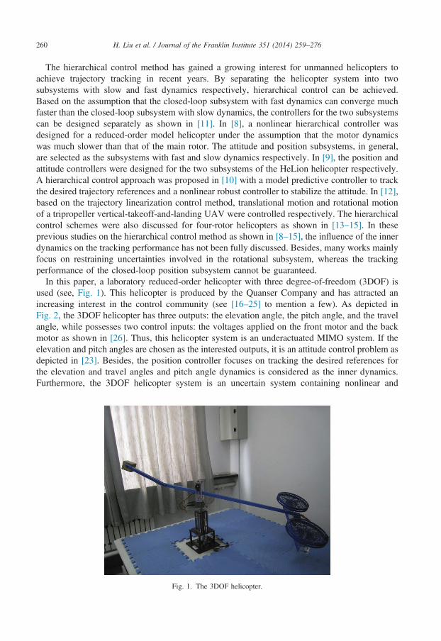
used (see, Fig. 1). This helicopter is produced by the Quanser Company and has attracted anincreasing interest in the control community (see [16–25] to mention a few). As depicted inFig. 2, the 3DOF helicopter has three outputs: the elevation angle, the pitch angle, and the travelangle, while possesses two control inputs: the voltages applied on the front motor and the backmotor as shown in [26]. Thus, this helicopter system is an underactuated MIMO system. If theelevation and pitch angles are chosen as the interested outputs, it is an attitude control problem asdepicted in [23]. Besides, the position controller focuses on tracking the desired references forthe elevation and travel angles and pitch angle dynamics is considered as the inner dynamics.Furthermore, the 3DOF helicopter system is an uncertain system containing nonlinear and

Fig. 1. The 3DOF helicopter.

Counterweight

Arm

Base

FrontMotor

BackMotorElevation

Axis

TravelAxis

PitchAxis

HelicopterFrame

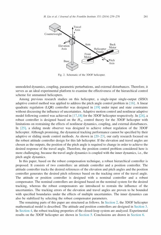
Fig. 2. Schematic of the 3DOF helicopter.

H. Liu et al. / Journal of the Franklin Institute 351 (2014) 259–276 261

unmodeled dynamics, coupling, parametric perturbations, and external disturbances. Therefore, itserves as an ideal experimental platform to examine the effectiveness of the hierarchical controlscheme for unmanned helicopters.

Among previous research studies on this helicopter, a single-input single-output (SISO)adaptive control method was applied to address the pitch angle control problem in [16]. A linearquadratic regulation (LQR) controller was designed in [19] under input and state constraintswithout discussing the influence of uncertainties. Adaptive motion control and nonlinear adaptivemodel following control was achieved in [17,18] for the 3DOF helicopter respectively. In [24], arobust controller is designed based on the H1 control theory for the 3DOF helicopter withlimitations on restraining the effects of nonlinear dynamics, coupling, and external disturbances.In [25], a sliding mode observer was designed to achieve robust regulation of the 3DOFhelicopter. Although promising, the dynamical tracking performance cannot be specified by theiradaptive or sliding mode control methods. As shown in [20–23], our early research focused onthe robust attitude controller design for this lab helicopter. If the elevation and travel angles arechosen as the outputs, the position of the pitch angle is required to change in order to achieve thedesired response of the travel angle. Therefore, the position control problem considered here ismore challenging, because the travel angle dynamics is coupled with the inner dynamics, i.e., thepitch angle dynamics.

In this paper, based on the robust compensation technique, a robust hierarchical controller isproposed. It consists of two controllers: an attitude controller and a position controller. Theattitude controller tracks the desired references of the elevation and pitch angles and the positioncontroller generates the desired pitch reference based on the tracking error of the travel angle.The attitude or position controller is designed with a nominal controller and a robustcompensator. The nominal controllers are designed based on the nominal system for the desiredtracking, whereas the robust compensators are introduced to restrain the influence of theuncertainties. The tracking errors of the elevation and travel angles are proven to be boundedwith specified boundaries under the effects of multiple uncertainties. The inner dynamics canalso be stabilized by selecting the robust compensator parameters.

The remaining parts of this paper are structured as follows. In Section 2, the 3DOF helicoptermathematical model is described. The attitude and position controllers are designed in Section 3.In Section 4, the robust tracking properties of the closed-loop system are analyzed. Experimentalresults on the 3DOF helicopter are shown in Section 5. Conclusions are drawn in Section 6.

H. Liu et al. / Journal of the Franklin Institute 351 (2014) 259–276262

2. Model description

As depicted in Fig. 2, the 3DOF helicopter includes two motors, a helicopter frame, an arm, acounterweight, and a base. The arm is free to rotate around the elevation and travel axes. At oneend of the arm, a counterweight is attached. The helicopter frame is attached at the other end ofthe arm and is free to rotate about its center (the pitch axis). The front and back motors areinstalled at the two ends of the helicopter frame, applied with voltages vf ðtÞ and vbðtÞrespectively. The twisting moment about the elevation axis can be generated by the sum of theforces produced by the front and back motors; the pitch motion is resulted from the differenceof the forces produced by the two motors; the position of the pitch angle can change thetorque about the travel axis as shown in [21]. The dynamical model of the elevation angle ξðtÞ,the pitch angle p(t), and the travel angle ψðtÞ can be described by the following equations (seealso in [17]):

€ξðtÞ ¼ a1ξðvf ðtÞ þ vbðtÞÞ cos pðtÞ þ a2ξ _ξðtÞ þ a3ξ sin ξðtÞ þ dξðtÞ;€pðtÞ ¼ a1pðvf ðtÞ�vbðtÞÞ þ a2p _pðtÞ þ a3p sin pðtÞ þ dpðtÞ;€ψ ðtÞ ¼ a1ψ ðvf ðtÞ þ vbðtÞÞ sin pðtÞ þ a1ψVop sin pðtÞ þ a2ψ _ψ ðtÞ þ dψ ðtÞ;

8><>: ð1Þ

where diði¼ ξ; p;ψÞ are external disturbances, a1i; a2iði¼ ξ; p;ψÞ; a3ξ, and a3p are the helicopterparameters, and Vop is the sum of quiescent voltages of the front and back motors, which is apositive constant. Let bξ ¼ a1ξ; bp ¼ a1p, and bψ ¼ a1ψVop. The parameters bi ði¼ ξ; p;ψÞ can besplit up into the given nominal parts and the uncertain parts, which are denoted by N and Δrespectively

bi ¼ bNi þ Δbi; i¼ ξ; p;ψ :

Define uξðtÞ ¼ vf ðtÞ þ vbðtÞ and upðtÞ ¼ vf ðtÞ�vbðtÞ. Then, the dynamical model (1) can berewritten as follows:

€ξðtÞ ¼ bNξ uξðtÞ þ qξðtÞ;€pðtÞ ¼ bNp upðtÞ þ qpðtÞ;€ψ ðtÞ ¼ bNψpðtÞ þ qψ ðtÞ;

8>><>>: ð2Þ

where qiðtÞ ði¼ ξ; p;ψÞ are the named equivalent disturbances and take the following forms:

qξðtÞ ¼ ðbξ cos pðtÞ�bNξ ÞuξðtÞ þ a2ξ _ξðtÞ þ a3ξ sin ξðtÞ þ dξðtÞ;qpðtÞ ¼ ðbp�bNp ÞupðtÞ þ a2p _pðtÞ þ a3p sin pðtÞ þ dpðtÞ;qψ ðtÞ ¼ a1ψuξðtÞ sin pðtÞ þ bψ sin pðtÞ�bNψpðtÞ þ a2ψ _ψ ðtÞ þ dψ ðtÞ:

8>><>>: ð3Þ

Remark 1. From Eq. (2), one can see that the desired response of the travel angle can beachieved by changing the position of the pitch angle. Thus, if the elevation and travel angles areselected as outputs, the pitch angle dynamics can be considered as the inner dynamics. Besides, itshould be noted that the nominal model (2) only contains primary linear terms, whereas otherknown terms are considered in equivalent disturbances in order to simplify the nominal model.

Assumption 1. The uncertain parameters a2i; bi ði¼ ξ; p;ψÞ; a3ξ, and a3p are bounded andbNi ði¼ ξ; p;ψÞ are positive and satisfy that jΔbijobNi .

H. Liu et al. / Journal of the Franklin Institute 351 (2014) 259–276 263

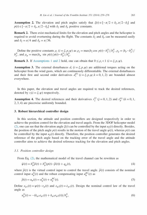
Assumption 2. The elevation and pitch angles satisfy that ξðtÞA ½�π=2þ δξ; π=2�δξ� andpðtÞA ½�π=2þ δp; π=2�δp� with δξ and δp positive constants.

Remark 2. There exist mechanical limits for the elevation and pitch angles and the helicopter isrequired to avoid overturning during the flight. The constants δξ and δp can be measured easilyand δξ ¼ π=4 and δp ¼ π=36.

Define the positive constants ρi ði¼ ξ; p;ψÞ as ρξ ¼maxjbξ cos pðtÞ�bNξ j=bNξ , ρp ¼ jbp�bNp j=bNp , and ρψ ¼maxjbψ sin pðtÞ=pðtÞ�bNψ j=bNψ .Remark 3. If Assumptions 1 and 2 hold, one can obtain that 0rρio1 ði¼ ξ; p;ψÞ.Assumption 3. The external disturbances di ði¼ ξ; p;ψÞ are additional torques acting on thehelicopter from the wind gusts, which are continuously differentiable. The external disturbancesand their first and second order derivatives dðkÞi ði¼ ξ; p;ψ ; k ¼ 0; 1; 2Þ are bounded almosteverywhere.

In this paper, the elevation and travel angles are required to track the desired references,denoted by riði¼ ξ;ψÞ respectively.Assumption 4. The desired references and their derivatives rðjÞξ ðj¼ 0; 1; 2Þ and rðkÞψ ðk¼ 0; 1;2; 3; 4Þ are piecewise uniformly bounded.

3. Robust hierarchical controller design

In this section, the attitude and position controllers are designed respectively in order toachieve the position control for the elevation and travel angels. From the 3DOF helicopter model(2), one can see that the elevation angle ξðtÞ can be controlled by the input uξðtÞ directly. Besides,the position of the pitch angle p(t) results in the motion of the travel angle ψðtÞ, whereas p(t) canbe controlled by the input upðtÞ directly. Therefore, the position controller generates the desiredreference of the pitch angle based on the tracking error of the travel angle and the attitudecontroller aims to achieve the desired reference tracking for the elevation and pitch angles.

3.1. Position controller design

From Eq. (2), the mathematical model of the travel channel can be rewritten as

€ψ ðtÞ ¼ bNψbpðtÞ þ bNψ ðpðtÞ�bpðtÞÞ þ qψ ðtÞ; ð4Þwhere bpðtÞ is the virtual control input to control the travel angle. bpðtÞ consists of the nominalcontrol input uNψ ðtÞ and the robust compensating input uRCψ ðtÞ asbpðtÞ ¼ uψ ðtÞ ¼ uNψ ðtÞ þ uRCψ ðtÞ: ð5ÞDefine eψ1ðtÞ ¼ ψðtÞ�rψ ðtÞ and eψ2ðtÞ ¼ _eψ1ðtÞ. Design the nominal control law of the travelangle as

uNψ ðtÞ ¼ �ðkψ1eψ1ðtÞ þ kψ2eψ2ðtÞÞ=bNψ ; ð6Þ

H. Liu et al. / Journal of the Franklin Institute 351 (2014) 259–276264

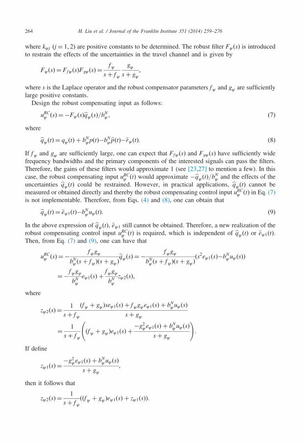
where kψ j ðj¼ 1; 2Þ are positive constants to be determined. The robust filter Fψ ðsÞ is introducedto restrain the effects of the uncertainties in the travel channel and is given by

Fψ ðsÞ ¼ Ffψ ðsÞFgψ ðsÞ ¼f ψ

sþ f ψ

gψsþ gψ

;

where s is the Laplace operator and the robust compensator parameters f ψ and gψ are sufficientlylarge positive constants.Design the robust compensating input as follows:

uRCψ ðsÞ ¼ �Fψ ðsÞbqψ ðsÞ=bNψ ; ð7Þwherebqψ ðtÞ ¼ qψ ðtÞ þ bNψpðtÞ�bNψbpðtÞ�€rψ ðtÞ: ð8ÞIf f ψ and gψ are sufficiently large, one can expect that Ffψ ðsÞ and Fgψ ðsÞ have sufficiently widefrequency bandwidths and the primary components of the interested signals can pass the filters.Therefore, the gains of these filters would approximate 1 (see [23,27] to mention a few). In thiscase, the robust compensating input uRCψ ðtÞ would approximate �bqψ ðtÞ=bNψ and the effects of theuncertainties bqψ ðtÞ could be restrained. However, in practical applications, bqψ ðtÞ cannot bemeasured or obtained directly and thereby the robust compensating control input uRCψ ðtÞ in Eq. (7)is not implementable. Therefore, from Eqs. (4) and (8), one can obtain thatbqψ ðtÞ ¼ €eψ1ðtÞ�bNψ uψ ðtÞ: ð9ÞIn the above expression of bqψ ðtÞ, €eψ1 still cannot be obtained. Therefore, a new realization of therobust compensating control input uRCψ ðtÞ is required, which is independent of bqψ ðtÞ or €eψ1ðtÞ.Then, from Eq. (7) and (9), one can have that

uRCψ ðsÞ ¼ � f ψgψbNψ ðsþ f ψ Þðsþ gψ Þ

bqψ ðsÞ ¼ � f ψgψbNψ ðsþ f ψ Þðsþ gψ Þ

ðs2eψ1ðsÞ�bNψuψ ðsÞÞ

¼ �f ψgψbNψ

eψ1ðsÞ þf ψgψbNψ

zψ2ðsÞ;

where

zψ2ðsÞ ¼1

sþ f ψ

ðf ψ þ gψ Þseψ1ðsÞ þ f ψgψeψ1ðsÞ þ bNψuψ ðsÞsþ gψ

¼ 1sþ f ψ

ðf ψ þ gψ Þeψ1ðsÞ þ�g2ψeψ1ðsÞ þ bNψ uψ ðsÞ

sþ gψ

!:

If define

zψ1ðsÞ ¼�g2ψeψ1ðsÞ þ bNψ uψ ðsÞ

sþ gψ;

then it follows that

zψ2ðsÞ ¼1

sþ f ψððf ψ þ gψ Þeψ1ðsÞ þ zψ1ðsÞÞ:

H. Liu et al. / Journal of the Franklin Institute 351 (2014) 259–276 265

Therefore, from the above expressions, uRCψ ðtÞ can be realized with zψ1ðtÞ and zψ2ðtÞ as_zψ1ðtÞ ¼ �gψzψ1ðtÞ�g2ψeψ1ðtÞ þ bNψuψ ðtÞ;_zψ2ðtÞ ¼ �f ψzψ2ðtÞ þ ðf ψ þ gψ Þeψ1ðtÞ þ zψ1ðtÞ;uRCψ ðtÞ ¼ f ψgψ ðzψ2ðtÞ�eψ1ðtÞÞ=bNψ :

8>><>>: ð10Þ

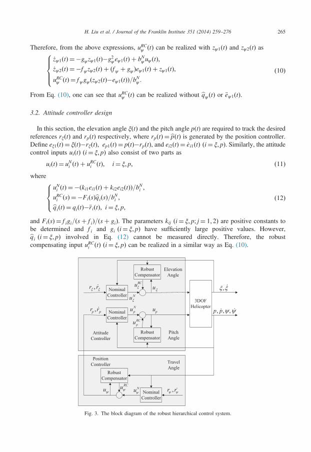
From Eq. (10), one can see that uRCψ ðtÞ can be realized without bqψ ðtÞ or €eψ1ðtÞ.3.2. Attitude controller design

In this section, the elevation angle ξðtÞ and the pitch angle p(t) are required to track the desiredreferences rξðtÞ and rpðtÞ respectively, where rpðtÞ ¼ bpðtÞ is generated by the position controller.Define eξ1ðtÞ ¼ ξðtÞ�rξðtÞ; ep1ðtÞ ¼ pðtÞ�rpðtÞ, and ei2ðtÞ ¼ _ei1ðtÞ ði¼ ξ; pÞ. Similarly, the attitudecontrol inputs uiðtÞ ði¼ ξ; pÞ also consist of two parts as

uiðtÞ ¼ uNi ðtÞ þ uRCi ðtÞ; i¼ ξ; p; ð11Þwhere

uNi ðtÞ ¼ �ðki1ei1ðtÞ þ ki2ei2ðtÞÞ=bNi ;uRCi ðsÞ ¼ �FiðsÞbqiðsÞ=bNi ;bqiðtÞ ¼ qiðtÞ�€riðtÞ; i¼ ξ; p;

8><>: ð12Þ

and FiðsÞ ¼ f igi=ðsþ f iÞ=ðsþ giÞ. The parameters kij ði¼ ξ; p; j¼ 1; 2Þ are positive constants tobe determined and f i and gi ði¼ ξ; pÞ have sufficiently large positive values. However,bqi ði¼ ξ; pÞ involved in Eq. (12) cannot be measured directly. Therefore, the robustcompensating input uRCi ðtÞ ði¼ ξ; pÞ can be realized in a similar way as Eq. (10).

3DOFHelicopter

, , ,p p

u ,

NominalController

RobustCompensator

NominalController

RobustCompensator

,p pr r

,r rNu

RCu

Npu

RCpu

pu

RobustCompensator

NominalController

,r rNuRCuu

TravelAngle

PitchAngle

ElevationAngle

AttitudeController

PositionController

Fig. 3. The block diagram of the robust hierarchical control system.

H. Liu et al. / Journal of the Franklin Institute 351 (2014) 259–276266

The block diagram of the robust hierarchical control system is depicted in Fig. 3.

Remark 4. The resulted hierarchical controller is a linear time-invariant one. In practicalapplications, it is easy to be implemented.

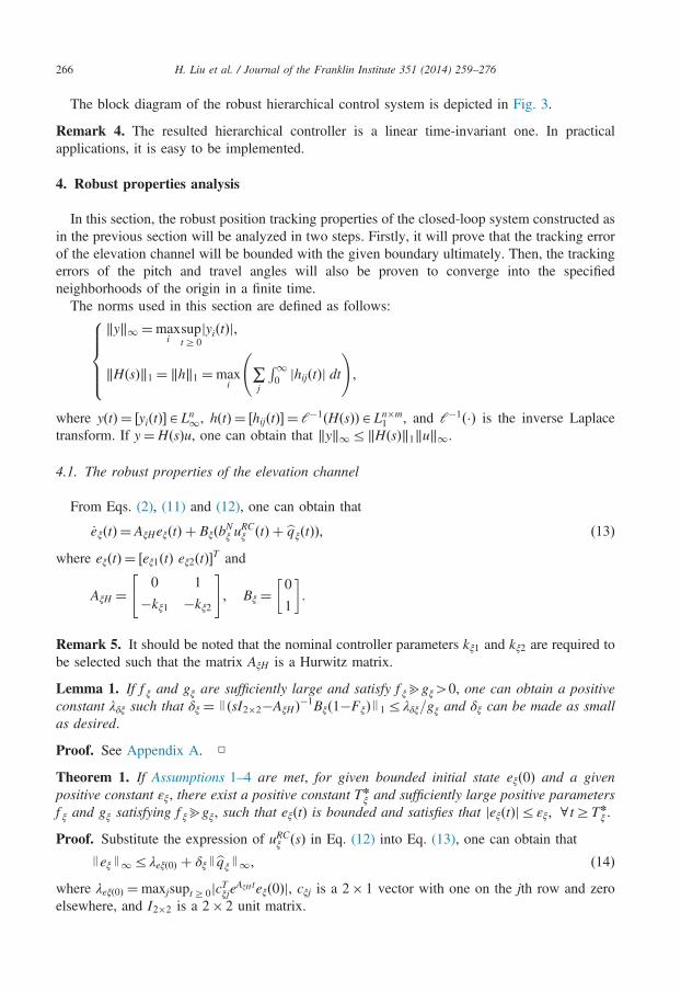
4. Robust properties analysis

In this section, the robust position tracking properties of the closed-loop system constructed asin the previous section will be analyzed in two steps. Firstly, it will prove that the tracking errorof the elevation channel will be bounded with the given boundary ultimately. Then, the trackingerrors of the pitch and travel angles will also be proven to converge into the specifiedneighborhoods of the origin in a finite time.The norms used in this section are defined as follows:

‖y‖1 ¼maxisuptZ0

jyiðtÞj;

‖HðsÞ‖1 ¼ ‖h‖1 ¼maxi

∑j

R10 jhijðtÞj dt

!;

8>>><>>>:where yðtÞ ¼ ½yiðtÞ�ALn1, hðtÞ ¼ ½hijðtÞ� ¼ ℓ�1ðHðsÞÞALn�m

1 , and ℓ�1ð�Þ is the inverse Laplacetransform. If y¼HðsÞu, one can obtain that ‖y‖1r‖HðsÞ‖1‖u‖1.

4.1. The robust properties of the elevation channel

From Eqs. (2), (11) and (12), one can obtain that

_eξðtÞ ¼ AξHeξðtÞ þ BξðbNξ uRCξ ðtÞ þ bqξðtÞÞ; ð13Þwhere eξðtÞ ¼ ½eξ1ðtÞ eξ2ðtÞ�T and

AξH ¼0 1

�kξ1 �kξ2

" #; Bξ ¼

0

1

� �:

Remark 5. It should be noted that the nominal controller parameters kξ1 and kξ2 are required tobe selected such that the matrix AξH is a Hurwitz matrix.

Lemma 1. If f ξ and gξ are sufficiently large and satisfy f ξbgξ40, one can obtain a positiveconstant λδξ such that δξ ¼ JðsI2�2�AξHÞ�1Bξð1�FξÞJ1rλδξ=gξ and δξ can be made as smallas desired.

Proof. See Appendix A. □

Theorem 1. If Assumptions 1–4 are met, for given bounded initial state eξð0Þ and a givenpositive constant εξ, there exist a positive constant Tn

ξ and sufficiently large positive parametersf ξ and gξ satisfying f ξbgξ, such that eξðtÞ is bounded and satisfies that jeξðtÞjrεξ; 8 tZTn

ξ .

Proof. Substitute the expression of uRCξ ðsÞ in Eq. (12) into Eq. (13), one can obtain that

Jeξ J1rλeξð0Þ þ δξ Jbqξ J1; ð14Þwhere λeξð0Þ ¼maxjsuptZ0jcTξjeAξHteξð0Þj, cξj is a 2� 1 vector with one on the jth row and zeroelsewhere, and I2�2 is a 2� 2 unit matrix.

H. Liu et al. / Journal of the Franklin Institute 351 (2014) 259–276 267

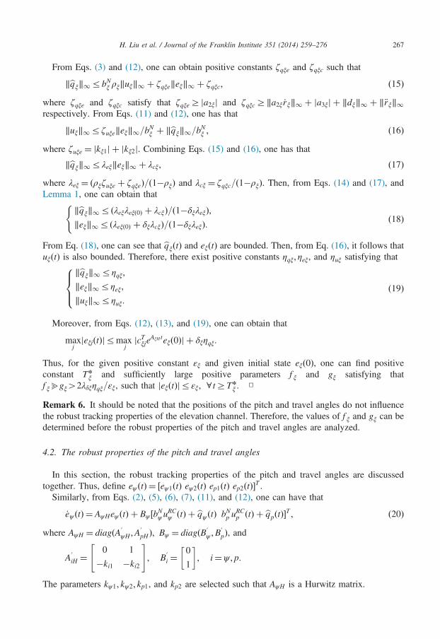
From Eqs. (3) and (12), one can obtain positive constants ζqξe and ζqξc such that

‖bqξ‖1rbNξ ρξ‖uξ‖1 þ ζqξe‖eξ‖1 þ ζqξc; ð15Þwhere ζqξe and ζqξc satisfy that ζqξeZ ja2ξj and ζqξcZ‖a2ξ _rξ‖1 þ ja3ξj þ ‖dξ‖1 þ ‖€rξ‖1respectively. From Eqs. (11) and (12), one has that

‖uξ‖1rζuξe‖eξ‖1=bNξ þ ‖bqξ‖1=bNξ ; ð16Þwhere ζuξe ¼ jkξ1j þ jkξ2j. Combining Eqs. (15) and (16), one has that

‖bqξ‖1rλeξ‖eξ‖1 þ λcξ; ð17Þwhere λeξ ¼ ðρξζuξe þ ζqξeÞ=ð1�ρξÞ and λcξ ¼ ζqξc=ð1�ρξÞ. Then, from Eqs. (14) and (17), andLemma 1, one can obtain that

‖bqξ‖1r ðλeξλeξð0Þ þ λcξÞ=ð1�δξλeξÞ;‖eξ‖1r ðλeξð0Þ þ δξλcξÞ=ð1�δξλeξÞ:

(ð18Þ

From Eq. (18), one can see that bqξðtÞ and eξðtÞ are bounded. Then, from Eq. (16), it follows thatuξðtÞ is also bounded. Therefore, there exist positive constants ηqξ; ηeξ, and ηuξ satisfying that

‖bqξ‖1rηqξ;

‖eξ‖1rηeξ;

‖uξ‖1rηuξ:

8><>: ð19Þ

Moreover, from Eqs. (12), (13), and (19), one can obtain that

maxjjeξjðtÞjrmax

jjcTξjeAξHteξð0Þj þ δξηqξ:

Thus, for the given positive constant εξ and given initial state eξð0Þ, one can find positiveconstant Tn

ξ and sufficiently large positive parameters f ξ and gξ satisfying thatf ξbgξ42λδξηqξ=εξ, such that jeξðtÞjrεξ; 8 tZTn

ξ . □

Remark 6. It should be noted that the positions of the pitch and travel angles do not influencethe robust tracking properties of the elevation channel. Therefore, the values of f ξ and gξ can bedetermined before the robust properties of the pitch and travel angles are analyzed.

4.2. The robust properties of the pitch and travel angles

In this section, the robust tracking properties of the pitch and travel angles are discussedtogether. Thus, define eψ ðtÞ ¼ ½eψ1ðtÞ eψ2ðtÞ ep1ðtÞ ep2ðtÞ�T .

Similarly, from Eqs. (2), (5), (6), (7), (11), and (12), one can have that

_eψ ðtÞ ¼ AψHeψ ðtÞ þ Bψ ½bNψ uRCψ ðtÞ þ bqψ ðtÞ bNp uRCp ðtÞ þ bqpðtÞ�T ; ð20Þ

where AψH ¼ diagðA′ψH ;A

′pHÞ; Bψ ¼ diagðB′

ψ ;B′pÞ, and

A′iH ¼

0 1

�ki1 �ki2

" #; B′

i ¼0

1

� �; i¼ ψ ; p:

The parameters kψ1; kψ2; kp1, and kp2 are selected such that AψH is a Hurwitz matrix.

H. Liu et al. / Journal of the Franklin Institute 351 (2014) 259–276268

Then, from Eqs. (7), (12), and (20), one can obtain that

‖eψ‖1rλeψð0Þ þ δψ‖Δψ‖1; ð21Þ

where Δψ ðtÞ ¼ ½bqψ ðtÞ bqpðtÞ=f ψ=gψ �T , δψ ¼maxfδ′ψ ; δ′pg, δ′ψ ¼ ‖ðsI2�2�A′ψHÞ�1B′

ψ ð1�Fψ Þ‖1,δ′p ¼ f ψgψ‖ðsI2�2�A′

pHÞ�1B′pð1�FpÞ‖1, λeψð0Þ ¼maxjsuptZ0jcTψ jeAψHteψ ð0Þj, and cψ j is a 4� 1

vector with one on the jth row and zeros elsewhere.

Lemma 2. If the robust compensator parameters f p; gp; f ψ , and gψ satisfy thatf ibgi40 ði¼ p;ψÞ and f p; gpbf ψ ; gψ , there exist positive constants λeψ ; λcψ ; λep, and λcp suchthat

‖bqψ‖1rλeψ‖eψ‖1 þ λcψ ;

‖bqp‖1rλepgψ f ψ‖eψ‖1 þ λcpgψ f ψ :

(ð22Þ

Proof. See Appendix B. □

Theorem 2. If Assumptions 1–4 hold, for a given positive constant εψ and given boundedinitial states of the pitch and travel angles, there exist a positive constant Tn

ψ and sufficientlylarge positive parameters f p; gp; f ψ , and gψ , which satisfy that f ibgi ði¼ p;ψÞ and f p; gpbf ψ ; gψ , such that the tracking error eψ is bounded and satisfies that jeψ ðtÞjrεψ ; 8 tZTn

ψ .

Proof. If f p and gp are much larger than f ψ and gψ , and f i ði¼ p;ψÞ are much larger thangi ði¼ p;ψÞ, one can obtain that δψ can be made as small as desired in a similar way. In this case,define λepψ ¼maxfλeψ ; λepg and λcpψ ¼maxfλcψ ; λcpg. Similarly with the elevation channel, fromEqs. (21) and (22), and Lemma 2, one can have that

‖bqψ‖1r ðλepψλeψð0Þ þ λcpψ Þ=ð1�δψλepψ Þ;‖eψ‖1r ðλeψð0Þ þ δψλcpψ Þ=ð1�δψλepψ Þ:

(ð23Þ

Therefore, one can see that bqψ ðtÞ and eψ ðtÞ are bounded, that is, one can find positive constantsηqψ and ηeψ satisfying that

‖bqψ‖1rηqψ ;

‖eψ‖1rηeψ :

(ð24Þ

Moreover, from Eqs. (7), (12), (20), and (24), one can have that

maxjjeψ jðtÞjrmax

jjcTψ jeAψHteψ ð0Þj þ δψηqψ :

For the given positive constant εψ and the given initial condition, one can find positive constantTnψ and positive parameters f p; gp; f ψ , and gψ with sufficiently large values and satisfy that

f ibgi ði¼ p;ψÞ and f p; gpbf ψ ; gψ , such that jeψ ðtÞjrεψ ; 8 tZTnψ . □

Remark 7. One can see that the tracking errors of the elevation and travel angles are proven toconverge into the given neighborhoods of the origin under the influence of various uncertainties.Furthermore, it should be noted that the robust tracking performance of the pitch angle can alsobe guaranteed by selecting the robust compensator parameters.

H. Liu et al. / Journal of the Franklin Institute 351 (2014) 259–276 269

5. Experimental results and discussions

In this section, results of real-time implementation of the proposed hierarchical controlleron the 3DOF helicopter are given to verify the effectiveness of the designed hierarchicalcontrol scheme. The three angles are measured by three encoders respectively. The effectiveresolutions of encoders for the elevation, travel, and pitch angles are 0.08791, 0.04391,and 0.08791 respectively as shown in [26]. The designed control scheme is implementedon a dSPACE system with a sampling time 10 ms. Then, the control signals are outputted to thetwo motors via amplifying. _rpðtÞ is estimated by the change rate of rpðtÞ. In practical applica-tions, let rpðsÞ ¼ bpðsÞ=ð0:01sþ 1Þ2 to reduce the noise in bpðsÞ. The nominal values of helicopterparameters are bNξ ¼ 0:0858, bNp ¼ 0:581, and bNψ ¼ 0:0825. The nominal controller para-meters are selected as kξ1 ¼ 2:79; kξ2 ¼ 2:38, kp1 ¼ 34:9; kp2 ¼ 31:9; kψ1 ¼ 0:496, andkψ2 ¼ 0:330. Choose the robust compensator parameters as f ξ ¼ 25; gξ ¼ 5; f p ¼ 25;gp ¼ 5; f ψ ¼ 1, and gψ ¼ 0:2 in order to guarantee the robust tracking performance of theclosed-loop system. In practical applications, by the following approach, one can try to make the3DOF helicopter avoiding overturning during the flight: generate the desired references withoutoverturning missions, make Assumption 4 hold, and try to make eið0Þ ði¼ ξ; p;ψÞ as small aspossible.

0 10 20 30 40 50−0.1

0

0.1

0.2

Time (s)

Ele

vatio

n an

gle

(deg

)

Reference signalElevation angle

0 10 20 30 40 50−0.05

0

0.05

0.1

Time (s)

Trav

el a

ngle

(deg

) Reference signalTravel angle

0 10 20 30 40 50

0

5

10

15

Time (s)

Pitc

h an

gle

(deg

) Reference signalPitch angle

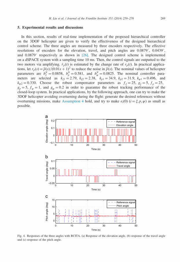
Fig. 4. Responses of the three angles with RCITA. (a) Response of the elevation angle, (b) response of the travel angleand (c) response of the pitch angle.

0 10 20 30 40 50−0.1

0

0.1

0.2

Time (s)

Ele

vatio

n an

gle

(deg

)

Reference signalElevation angle

0 10 20 30 40 50−0.1

0

0.1

0.2

Time (s)

Trav

el a

ngle

(deg

) Reference signalTravel angle

0 10 20 30 40 50

0

5

10

15

Time (s)

Pitc

h an

gle

(deg

) Reference signalPitch angle

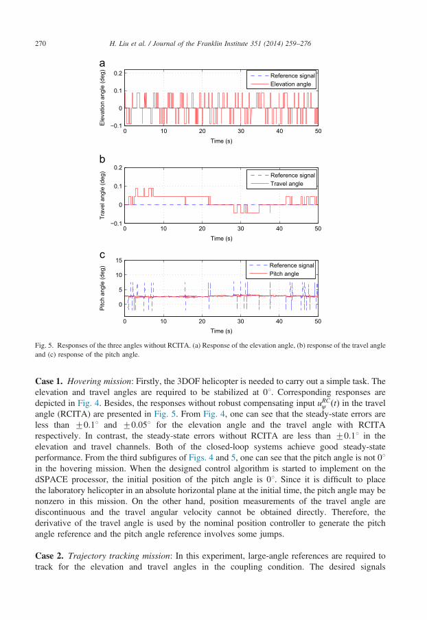
Fig. 5. Responses of the three angles without RCITA. (a) Response of the elevation angle, (b) response of the travel angleand (c) response of the pitch angle.

H. Liu et al. / Journal of the Franklin Institute 351 (2014) 259–276270

Case 1. Hovering mission: Firstly, the 3DOF helicopter is needed to carry out a simple task. Theelevation and travel angles are required to be stabilized at 01. Corresponding responses aredepicted in Fig. 4. Besides, the responses without robust compensating input uRCψ ðtÞ in the travelangle (RCITA) are presented in Fig. 5. From Fig. 4, one can see that the steady-state errors areless than 70.11 and 70.051 for the elevation angle and the travel angle with RCITArespectively. In contrast, the steady-state errors without RCITA are less than 70.11 in theelevation and travel channels. Both of the closed-loop systems achieve good steady-stateperformance. From the third subfigures of Figs. 4 and 5, one can see that the pitch angle is not 01in the hovering mission. When the designed control algorithm is started to implement on thedSPACE processor, the initial position of the pitch angle is 01. Since it is difficult to placethe laboratory helicopter in an absolute horizontal plane at the initial time, the pitch angle may benonzero in this mission. On the other hand, position measurements of the travel angle arediscontinuous and the travel angular velocity cannot be obtained directly. Therefore, thederivative of the travel angle is used by the nominal position controller to generate the pitchangle reference and the pitch angle reference involves some jumps.

Case 2. Trajectory tracking mission: In this experiment, large-angle references are required totrack for the elevation and travel angles in the coupling condition. The desired signals

0 50 100 150 200−10

0

10

20

Time (s)

Ele

vatio

n an

gle

(deg

)

Reference signalElevation angle

0 50 100 150 2000

10

20

30

Time (s)

Trav

el a

ngle

(deg

) Reference signalTravel angle

0 50 100 150 200

−10

0

10

20

30

Time (s)

Pitc

h an

gle

(deg

) Reference signalPitch angle

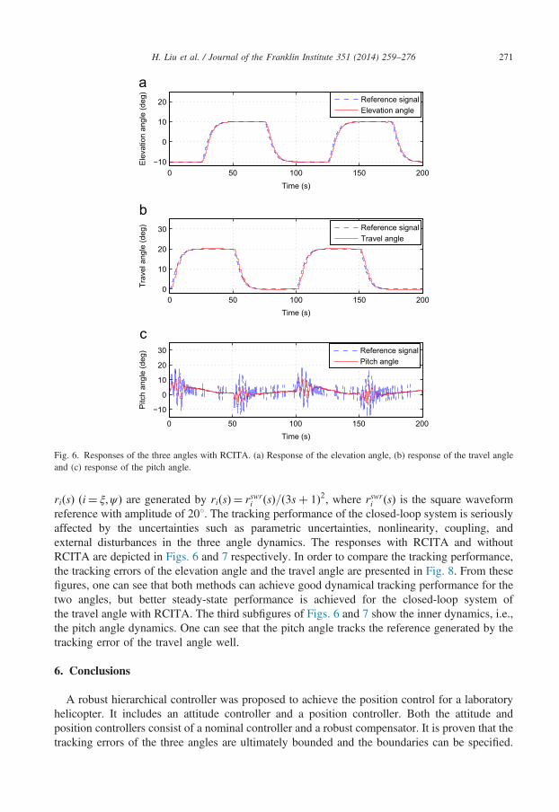
Fig. 6. Responses of the three angles with RCITA. (a) Response of the elevation angle, (b) response of the travel angleand (c) response of the pitch angle.

H. Liu et al. / Journal of the Franklin Institute 351 (2014) 259–276 271

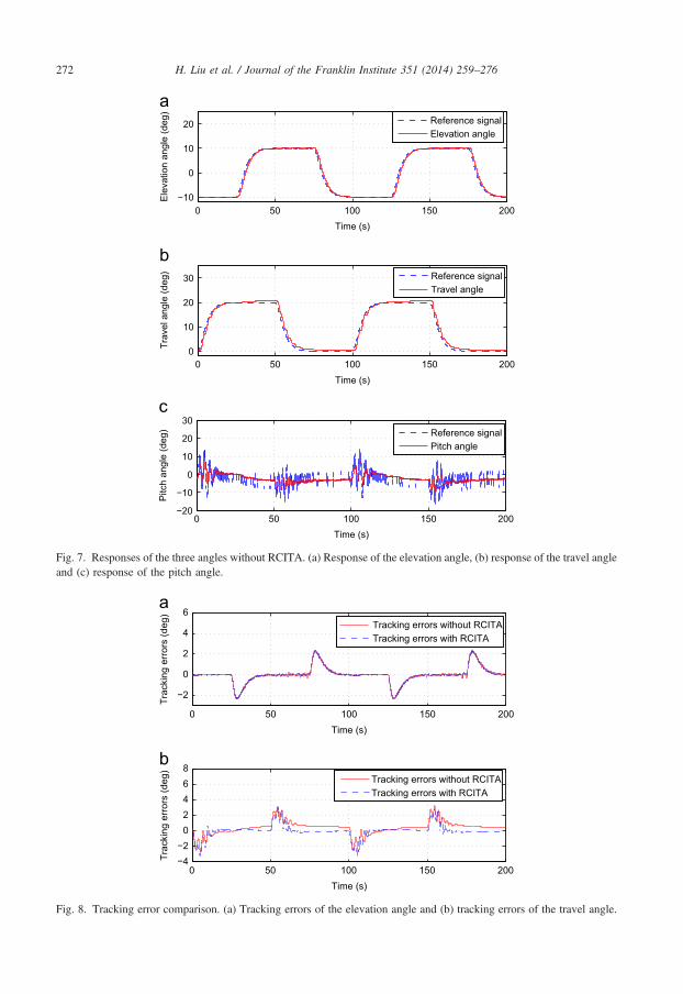
riðsÞ ði¼ ξ;ψÞ are generated by riðsÞ ¼ rswri ðsÞ=ð3sþ 1Þ2, where rswri ðsÞ is the square waveformreference with amplitude of 201. The tracking performance of the closed-loop system is seriouslyaffected by the uncertainties such as parametric uncertainties, nonlinearity, coupling, andexternal disturbances in the three angle dynamics. The responses with RCITA and withoutRCITA are depicted in Figs. 6 and 7 respectively. In order to compare the tracking performance,the tracking errors of the elevation angle and the travel angle are presented in Fig. 8. From thesefigures, one can see that both methods can achieve good dynamical tracking performance for thetwo angles, but better steady-state performance is achieved for the closed-loop system ofthe travel angle with RCITA. The third subfigures of Figs. 6 and 7 show the inner dynamics, i.e.,the pitch angle dynamics. One can see that the pitch angle tracks the reference generated by thetracking error of the travel angle well.

6. Conclusions

A robust hierarchical controller was proposed to achieve the position control for a laboratoryhelicopter. It includes an attitude controller and a position controller. Both the attitude andposition controllers consist of a nominal controller and a robust compensator. It is proven that thetracking errors of the three angles are ultimately bounded and the boundaries can be specified.

0 50 100 150 200−10

0

10

20

Time (s)

Ele

vatio

n an

gle

(deg

)

Reference signalElevation angle

0 50 100 150 2000

10

20

30

Time (s)

Trav

el a

ngle

(deg

) Reference signalTravel angle

0 50 100 150 200−20

−10

0

10

20

30

Time (s)

Pitc

h an

gle

(deg

) Reference signalPitch angle

Fig. 7. Responses of the three angles without RCITA. (a) Response of the elevation angle, (b) response of the travel angleand (c) response of the pitch angle.

0 50 100 150 200

−2

0

2

4

6

Time (s)

Trac

king

err

ors

(deg

)

Tracking errors without RCITATracking errors with RCITA

0 50 100 150 200−4−2

02468

Time (s)

Trac

king

err

ors

(deg

)

Tracking errors without RCITATracking errors with RCITA

Fig. 8. Tracking error comparison. (a) Tracking errors of the elevation angle and (b) tracking errors of the travel angle.

H. Liu et al. / Journal of the Franklin Institute 351 (2014) 259–276272

H. Liu et al. / Journal of the Franklin Institute 351 (2014) 259–276 273

Experimental results on the 3DOF helicopter demonstrated the effectiveness of the proposedcontrol method.

Acknowledgments

This work was supported by the National Natural Science Foundation of China under Grants61174067, 61203071, and 61374054, as well as Shaanxi Province Natural Science FoundationResearch Projection under Grants 2013JQ8038.

Appendix A. Proof of Lemma 1

Let

dξHðsÞ ¼ detðsI2�2�AξHÞ ¼ ðsþ sξ1Þðsþ sξ2Þ ¼ ðs2 þ kξ2sþ kξ1Þ; ðA:1Þand

χξðsÞ ¼ ðsþ 1ÞðsI2�2�AξHÞ�1�I2�2: ðA:2ÞIt follows that

δξr ð‖χξðsÞ‖1 þ ‖I2�2‖1Þ‖Bξ‖1 ð1�FξÞ1

sþ 1

���� ����1

: ðA:3Þ

The term ðsI2�2�AξHÞ�1 can be expressed as

ðsI2�2�AξHÞ�1 ¼NξHðsÞdξHðsÞ

; ðA:4Þ

where

NξHðsÞ ¼sþ kξ2 1

�kξ1 s

" #: ðA:5Þ

Let χξðsÞ ¼ ½χξ;jkðsÞ�2�2. Then, χξ;jkðsÞ has the following form:

χξ;jkðsÞ ¼χξ1ξ;jk

sþ sξ1þ χξ2ξ;jk

sþ sξ2;

where χξ1ξ;jk and χξ2ξ;jk are constants. It follows that

‖χξðsÞ‖1rmaxj

∑2

k ¼ 1‖χξ;jkðsÞ‖1

� �rmax

j∑2

k ¼ 1

���χξ1ξ;jksξ1

���þ ���χξ2ξ;jksξ2

��� !:

Therefore, there exists a positive constant λ1δξ, such that

ð‖χξðsÞ‖1 þ ‖I2�2‖1Þrλ1δξ: ðA:6ÞFurthermore, one can obtain that ‖Bξ‖1 ¼ 1 and

ð1�FξÞ1

sþ 1

���� ����1

¼ηf ξ

sþ f ξþ

ηgξsþ gξ

þ 1gξ

η1sþ 1

���� ����1

;

H. Liu et al. / Journal of the Franklin Institute 351 (2014) 259–276274

where

ηf ξ ¼�f ξgξ=ðf ξ�gξÞ=ðf ξ�1Þ;ηgξ ¼ f ξgξ=ðf ξ�gξÞ=ðgξ�1Þ;η1 ¼ ð�f ξgξ�g2ξ þ gξÞ=ðf ξ�1Þ=ðgξ�1Þ:

8>><>>:If the positive constants f ξ and gξ are sufficiently large, one can obtain a positive constant λ2δξsuch that

‖Bξ‖1 ð1�FξÞ 1sþ sa

���� ����1

rλ2δξgξ

: ðA:7Þ

Let λδξ ¼ λ1δξλ2δξ. From Eqs. (A.(3), A.6), and (A.7), one can obtain that

δξrλδξgξ

: ðA:8Þ

If the positive constants f ξ and gξ are sufficiently large, the constant λδξ is irrelevant of f ξ and gξ.In this case, if gξ is sufficiently large, the variable δξ can be made as small as desired. It followsthat Lemma 1 can hold.

Appendix B. Proof of Lemma 2

From Eqs. (5) and (6), one has that

rpðtÞ ¼ uψ ðtÞ ¼ �ðkψ1eψ1ðtÞ þ kψ2eψ2ðtÞÞ=bNψ þ uRCψ ðtÞ: ðB:1ÞFrom Eqs. (3), (8), and (19), one can obtain that

‖bqψ‖1rζqψe‖eψ‖1 þ ρψbNψ‖rp‖1 þ ζqψc; ðB:2Þ

where ζqψe and ζqψc satisfy that

ζqψeZ ja2ψ j þ bNψ þ ρψbNψ ;

ζqψcZ ja1ψ jηuξ þ ja2ψ j‖_rψ‖1 þ ‖€rψ‖1 þ ‖dψ‖1:

(Combining Eqs. ((7) and B.2), one can have that

‖uRCψ ‖1rζqψe‖eψ‖1=bNψ þ ρψ‖rp‖1 þ ζqψc=bNψ : ðB:3Þ

Let

λr0ep ¼ ðjkψ1j þ jkψ2j þ ζqψeÞ=bNψ =ð1�ρψ Þ;λr0cp ¼ ζqψc=b

Nψ=ð1�ρψ Þ:

(Then, from Eqs. (B.(1) and B.3), one can obtain that

‖rp‖1rλr0ep‖eψ‖1 þ λr0cp: ðB:4ÞDifferentiating both sides of Eq. (B.1) leads to

_rpðtÞ ¼ �ðkψ1eψ2ðtÞ þ kψ2 _eψ2ðtÞÞ=bNψ þ _uRCψ ðtÞ: ðB:5ÞBesides, from Eq. (20), one has that

_eψ2ðtÞ ¼ �kψ1eψ1ðtÞ�kψ2eψ2ðtÞ þ bNψ uRCψ ðtÞ þ bqψ ðtÞ: ðB:6Þ

H. Liu et al. / Journal of the Franklin Institute 351 (2014) 259–276 275

From Eqs. ((7), B.5), and (B.6), one can obtain positive constants ζr1ep; ζr1qp, and ζr1cp such that

‖_rp‖1rζr1ep‖eψ‖1 þ ζr1qp‖1�Fψ‖1‖bqψ‖1 þ ‖ _uRCψ ‖1 þ ζr1cp: ðB:7ÞFrom Eq. (7), one has that

‖ _uRCψ ‖1rgψ‖f ψ

sþ f ψ

s

sþ gψ‖1‖bqψ‖1=bNψ rgψ‖1�Fgψ‖1‖bqψ‖1=bNψ :

It follows that

‖_rp‖1rζr1ep‖eψ‖1 þ ζr1qp‖1�Fψ‖1‖bqψ‖1 þ gψ‖1�Fgψ‖1‖bqψ‖1=bNψ þ ζr1cp: ðB:8ÞMoreover, if the positive parameters f ψ and gψ are sufficiently large, one can see that

‖1�Fψ‖1 and ‖1�Fgψ‖1 are bounded. Thus, there exist positive constants λr1ep and λr1cpsatisfying

λr1epgψ4ζr1ep þ ðζr1qp‖1�Fψ‖1 þ gψ‖1�Fgψ‖1=bNψ Þðζqψe þ ρψbNψ λr0epÞ;

λr1cpgψ4ζr1cp þ ðζr1qp‖1�Fψ‖1 þ gψ‖1�Fgψ‖1=bNψ Þðζqψc þ ρψbNψ λr0cpÞ:

(Then, from Eqs. (B.(2), B.4), and (B.8), it follows that

‖_rp‖1rλr1epgψ‖eψ‖1 þ λr1cpgψ : ðB:9ÞSimilarly, there exist positive constants λr2ep and λr2cp such that

‖€rp‖1rλr2epgψ f ψ‖eψ‖1 þ λr2cpgψ f ψ : ðB:10ÞFrom Eqs. (B.(2) and B.4), one can obtain positive constants λeψ and λcψ such that

‖bqψ‖1rλeψ‖eψ‖1 þ λcψ : ðB:11ÞFurthermore, from Eqs. (3), (11), and (12), there exist positive constants ζr1p; ζr2p; ζrep, and

ζrcp such that

‖bqp‖1rζr1p‖_rp‖1 þ ζr2p‖€rp‖1 þ ζrep‖eψ‖1 þ ζrcp: ðB:12ÞIf f ψ and gψ are sufficiently large and satisfy that f ψbgψ40, from Eqs. (B.(9), B.10), and(B.12), one can obtain positive constants λep and λcp such that

‖bqp‖1rλepgψ f ψ‖eψ‖1 þ λcpgψ f ψ : ðB:13ÞFrom Eqs. (B.(11) and B.13), one can see that Lemma 2 holds.

References

[1] M.S. Mahmoud, A.B. Koesdwiady, Improved digital tracking controller design for pilot-scale unmanned helicopter,Journal of The Franklin Institute 349 (2012) 42–58.

[2] R. Mahony, V. Kumar, P. Corke, Multirotor aerial vehicles: modeling, estimation, and control of quadrotor, IEEERobotics and Automation Magazine 19 (3) (2012) 20–32.

[3] C. Aguilar-Ibanez, H. Sira-Ramirez, M.S. Suarez-Castanon, E. Martinez-Navarro, M.A. Moreno-Armendariz,The trajectory tracking problem for an unmanned four-rotor system: flatness-based approach, International Journalof Control 85 (1) (2012) 69–77.

[4] J.R. Majhi, R. Ganguli, Helicopter blade flapping with and without small angle assumption in the presence ofdynamic stall, Applied Mathematical Modelling 34 (12) (2010) 3726–3740.

H. Liu et al. / Journal of the Franklin Institute 351 (2014) 259–276276

[5] M. Sayed, M. Kamel, Stability study and control of helicopter blade flapping vibrations, Applied MathematicalModelling 35 (6) (2011) 2820–2837.

[6] L. Marconi, R. Naldi, Robust full degree-of-freedom tracking control of a helicopter, Automatica 43 (2007)1909–1920.

[7] L. Derafa, A. Benallegue, L. Fridman, Super twisting control algorithm for the attitude tracking of a four rotorsUAV, Journal of The Franklin Institute 349 (2012) 685–699.

[8] J.C.A. Vilchis, B. Brogliato, A. Dzul, R. Lozano, Nonlinear modelling and control of helicopters, Automatica 39(2003) 1583–1596.

[9] K. Peng, G. Cai, B.M. Chen, M. Dong, K.Y. Lum, T.H. Lee, Design and implementation of an autonomous flightcontrol law for a UAV helicopter, Automatica 45 (2009) 2333–2338.

[10] G.V. Raffo, M.G. Ortega, F.R. Rubio, An integral predictive/nonlinear H1 control structure for a quadrotorhelicopter, Automatica 46 (2010) 29–39.

[11] S. Bertrand, N. Guenard, T. Hamel, H. Piet-Lahanier, L. Eck, A hierarchical controller for miniature VTOL UAVs:design and stability analysis using singular perturbation theory, Control Engineering Practice 19 (2011) 1099–1108.

[12] R. Huang, Y. Liu, J.J. Zhu, Guidance, navigation, and control system design for tripropeller vertical-takeoff-and-landing unmanned air vehicle, Journal of Aircraft 46 (2009) 1837–1856.

[13] A. Das, K. Subbarao, F. Lewis, Dynamic inversion with zero-dynamics stabilization for quadrotor control, IETControl Theory and Applications 3 (2009) 303–314.

[14] Z. Zuo, Trajectory tracking control design with command-filtered compensation for a quadrotor, IET Control Theoryand Applications 4 (2010) 2343–2355.

[15] R. Mahony, V. Kumar, P. Corke, Multirotor aerial vehicles: modeling, estimation, and control of quadrotor, IEEERobotics and Automation Magazine 19 (2012) 20–32.

[16] A.T. Kutay, A.J. Calise, M. Idan, N. Hovakimyan, Experimental results on adaptive output feedback control using alaboratory model helicopter, IEEE Transactions on Control Systems Technology 13 (2005) 196–202.

[17] B. Andrievsky, D. Peaucelle, A.L. Fradkov, Adaptive control of 3DOF motion for LAAS helicopter benchmark:design and experiments, in: Proceedings of American Control Conference, New York, USA, 2007, pp. 3312–3317.

[18] M. Ishitobi, M. Nishi, K. Nakasaki, Nonlinear adaptive model following control for a 3-DOF tandem-rotor modelhelicopter, Control Engineering Practice 18 (2010) 936–943.

[19] T. Kiefer, K. Graichen, A. Kugi, Trajectory tracking of a 3DOF laboratory helicopter under input and stateconstraints, IEEE Transactions on Control Systems Technology 18 (2010) 944–952.

[20] Y. Yu, Y.S. Zhong, Robust attitude control of a 3DOF helicopter with multi-operation points, Journal of SystemsScience and Complexity 22 (2009) 207–219.

[21] B. Zheng, Y. Zhong, Robust attitude regulation of a 3-DOF helicopter benchmark: theory and experiments, IEEETransactions on Industrial Electronics 58 (2011) 660–670.

[22] H. Liu, Y. Yu, G. Lu, Y. Zhong, Robust LQR attitude control of 3DOF helicopter, in: Proceedings of ChineseControl Conference, Beijing, China, 2010, pp. 529–534.

[23] H. Liu, G. Lu, Y. Zhong, Robust LQR attitude control of a 3-DOF lab helicopter for aggressive maneuvers, IEEETransactions on Industrial Electronics 60 (2013) 4627–4636.

[24] I.M. Meza-Sanchez, L.T. Aguilar, A. Shiriaev, L. Freidovich, Y. Orlov, Periodic motion planning and nonlineartracking control of a 3-DOF underactuated helicopter, International Journal of Systems Science 42 (2011) 829–838.

[25] A. Loza, H. Rios, A. Rosales, Robust regulation for a 3-DOF helicopter via sliding-mode observation andidentification, Journal of The Franklin Institute 349 (2012) 700–718.

[26] J. Apkarian, Position Control 3-DOF Helicopter Reference Manual, The Quanser Consulting IncorporatedCompany, Markham, 2006.

[27] Y. Zhong, Robust output tracking control of SISO plants with multiple operating points and with parametric andunstructured uncertainties, International Journal of Control 75 (2002) 219–241.