Manuscript submitted to doi:10.3934/xx.xx.xx.xxAIMS’ JournalsVolume X, Number 0X, XX 200X pp. X–XX

ROBUST AND STABLE REGION-OF-INTEREST1

TOMOGRAPHIC RECONSTRUCTION USING A ROBUST2

WIDTH PRIOR3

Bart Goossens∗

imec-IPI-Ghent UniversityB9000 Gent, Belgium

Demetrio Labate and Bernhard G Bodmann

Department of MathematicsUniversity of Houston

Houston, TX 77204-3008, USA

(Communicated by the associate editor name)

Abstract. Region-of-interest computed tomography (ROI CT) aims at re-

constructing a region within the field of view by using only ROI-focused pro-jections. The solution of this inverse problem is challenging and methods of

tomographic reconstruction that are designed to work with full projection data

may perform poorly or fail completely when applied to this setting. In thiswork, we study the ROI CT problem in the presence of measurement noise

and formulate the reconstruction problem by relaxing data fidelity and con-

sistency requirements. Under the assumption of a robust width prior thatprovides a form of stability for data satisfying appropriate sparsity norms, we

derive reconstruction performance guarantees and controllable error bounds.Based on this theoretical setting, we introduce a novel iterative reconstruction

algorithm from ROI-focused projection data that is guaranteed to converge

with controllable error while satisfying predetermined fidelity and consistencytolerances. Numerical tests on experimental data show that our algorithm for

ROI CT performs very competitively with respect to state-of-the-art methods

especially when the ROI radius is small.

1. Introduction. Computed tomography (CT) is a non-invasive scanning method4

that is widely employed in medical and industrial imaging to reconstruct the un-5

known interior structure of an object from a collection of projection images. In6

many applications of CT, one is interested in recovering only a small region-of-7

interest (ROI) within the field of view at a high resolution level. Such applications8

include contrast-enhanced cardiac imaging and surgical implant procedures where9

it is necessary to ensure the accurate positioning of an implant. The ability of per-10

forming accurate ROI reconstruction using only ROI-focused scanning offers several11

potential advantages, including the reduction of radiation dose, the shortening of12

2010 Mathematics Subject Classification. Primary: 44A12, 65R32; Secondary: 92C55.Key words and phrases. Region-of-interest tomography, robust width, sparsity, iterative recon-

struction, convex optimization.The second author is supported by NSF grants DMS 1720487 and 1720452 and the third author

is supported by NSF grant DMS 1412524.∗ Corresponding author: xxxx.

1

2 BART GOOSSENS AND DEMETRIO LABATE AND BERNHARD G BODMANN

Region of Interest

Source

Detector

Region of Interest

Source

DetectorKnown subregion

Region of Interest

Source

Detector

(a) (b) (c)

Figure 1. Illustrations of recoverable regions for truncated pro-jection data: (a) initial DBP methods [3, 5, 6] require at least oneprojection view in which the complete object is covered, (b) inte-rior reconstruction is possible given a known subregion [4, 7, 8, 9]and (c) no assumptions are made other than that the shape of theROI is convex and approximate sparsity within a ridgelet domain(this paper). The gray dashed line indicates the measured area onthe detector array for one particular source angle.

scanning time and the possibility of imaging large objects. However, when pro-1

jections are truncated as is the case for ROI-focused scanning, the reconstruction2

problem is ill-posed [1] and conventional reconstruction algorithms, e.g., Filtered3

Back-Projection, may perform poorly or fail. Further, it is known that the interior4

problem, where projections are known only for rays intersecting a region strictly5

inside the field of view, is in general not uniquely solvable [1].6

Existing methods for local CT reconstruction typically require restrictions on the7

geometry and location of the ROI or some prior knowledge of the solution inside8

the ROI. For instance, analytic ROI reconstruction formulas associated with the9

differentiated back-projection (DBP) framework [2, 3, 4] require that there exists a10

projection angle θ such that for angles in its vicinity, complete (i.e. non-truncated)11

projection data is available [3, 5, 6]; hence such formulas may fail if the ROI is12

located strictly inside the scanned object (see illustration in Fig 1). Other results13

show that restrictions on the ROI location can be removed provided that the density14

function to be recovered is known on a subregion inside the ROI (Fig. 1(b)) or has15

a special form, e.g., it is piecewise constant inside the ROI [4, 7, 8, 9]. However,16

even when ROI reconstruction is theoretically guaranteed, stable numerical recovery17

often requires a regularization, e.g., L1-norm minimization of the gradient image18

[4, 8] or singular value decomposition of the truncated Hilbert transform [9, 10].19

We also recall that methods from deep learning have been recently proposed for20

problems of tomographic reconstruction from incomplete data, especially for the21

limited-view case [11, 12, 13, 14]. In these approaches, a neural network is trained to22

extrapolate the missing projection data. Despite yielding high quality visual results,23

these methods lack the theoretical framework to give performance guarantees on the24

reconstruction (e.g., in terms of noise robustness and accuracy).25

One major aim of this paper is to derive reconstruction performance guarantees26

for ROI CT in the setting of noisy projection data. To this end, we introduce a27

novel theoretical approach based on a robust width prior assumption [15, 16], a28

method guaranteeing a form of geometrical stability for data satisfying an appro-29

priate sparsity condition. Using this framework, we can establish error bounds for30

reconstruction from noisy data in both the image and projection spaces. A novelty31

of our approach is that the image and projection data are handled jointly in the re-32

covery, with sparsity prior in both domains. Moreover, as explained below, fidelity33

ROBUST AND STABLE REGION-OF-INTEREST TOMOGRAPHIC RECONSTRUCTION 3

and consistency requirements are relaxed to handle the presence of noise leading to1

an extrapolation scheme for the missing projection data that is guided by the data2

fidelity and consistency terms. Our implementation of the recovery is then achieved3

by an iterative, Bregman-based convex optimization algorithm consistent with our4

theoretical setting.5

Iterative algorithms for CT reconstruction found in the literature typically fo-6

cus on the minimization of a fidelity norm measuring the distance between observed7

and reconstructed projections within the ROI (i.e., not taking the image domain re-8

construction error into account); see, for example, the simultaneous iterative recon-9

struction technique (SIRT) [17], the maximum likelihood expectation-maximization10

algorithm (MLEM) [18], the least-squares Conjugate Gradient (LSCG) method [19,11

20], and Maximum Likelihood for Transmission Tomography (MLTR) [21]. We ob-12

served that the performance of these methods on ROI CT reconstruction, in the13

presence of measurement noise, is increasingly less reliable as the ROI size decreases.14

To overcome this issue, our method relaxes the consistency requirement of the recon-15

struction algorithm since measured data may fall outside the range of the forward16

projection due to the noise. This added flexibility is especially advantageous when17

another prior, namely the sparsity of solution, is included.18

Sparsity assumptions have already been applied in the literature to reduce mea-19

sured data and mitigate the effect of noise in the recovery from linear measure-20

ments [22, 23]. However, most theoretical results are based on randomized mea-21

surements that are different in nature from the deterministic way the projection22

data is obtained in CT. Nevertheless, it is generally agreed that sparsity is a power-23

ful prior in the context of tomography when conventional recovery methods lead to24

ill-posedness [24, 25]. In this paper, we incorporate an assumption of approximate25

sparseness by minimizing the ℓ1 norm of the ridgelet coefficients of the reconstructed26

image (i.e., the 1D wavelet coefficients of the reconstructed projection data, where27

the wavelet transform is applied along the detector array) while retaining given28

tolerances for fidelity and consistency of the recovered data. One of our main re-29

sults is that we can guarantee that our iterative algorithm reaches an approximate30

minimizer with the prescribed tolerances within a finite number of steps. To val-31

idate our method, we also demonstrate the application of our algorithm for ROI32

reconstruction from noisy projection data in the 2D fan-beam reconstruction. Our33

approach yields highly accurate reconstructions within the ROI and outperforms34

existing algorithms especially for ROIs with a small radius.35

The remainder of the paper is organized as follows. In Sec. 2, we formulate the36

ROI reconstruction problem and introduce a notion of data fidelity and consistency37

in the context of ROI CT. In Sec. 3, we recall the definition of robust width and38

prove that, under appropriate sparsity assumptions on the data, it is feasible to find39

an approximate solution of a noisy linear problem with controllable error. Based on40

this formulation, in Sec. 4 we introduce a convex optimization approach to solve the41

ROI CT problem from noisy truncated projections and show that we can control42

reconstruction error under predetermined fidelity and consistency tolerances. We43

finally present numerical demonstrations of our method in Sec. 5.44

2. Data consistency and fidelity in the ROI reconstruction problem. In45

this section, we introduce the main notations used for ROI CT and show how46

the non-uniqueness of the reconstruction problem in the presence of noise leads to47

4 BART GOOSSENS AND DEMETRIO LABATE AND BERNHARD G BODMANN

two requirements, i.e., data fidelity and data consistency requirements, that cannot1

necessarily be satisfied at the same time but can be relaxed.2

Let W denote a projection operator mapping a density function f on R2 into3

a set of its linear projections. A classical example of such operator is the Radon4

transform, defined by5

Wradonf(θ, τ) =

∫ℓ(θ,τ)

f(x) dx,

where ℓ(θ, τ) = {x ∈ R2 : x · eθ = τ} is the line that is perpendicular to eθ =6

(cos θ, sin θ) ∈ S1 with (signed) distance τ ∈ R from the origin. This transform7

maps f ∈ L2(R2) into the set of its line integrals defined on the tangent space of8

the circle9

T = {(θ, τ) : θ ∈ [0, π), τ ∈ R}.

Another classical example of a projection operator W is the fan-beam transform10

[26].11

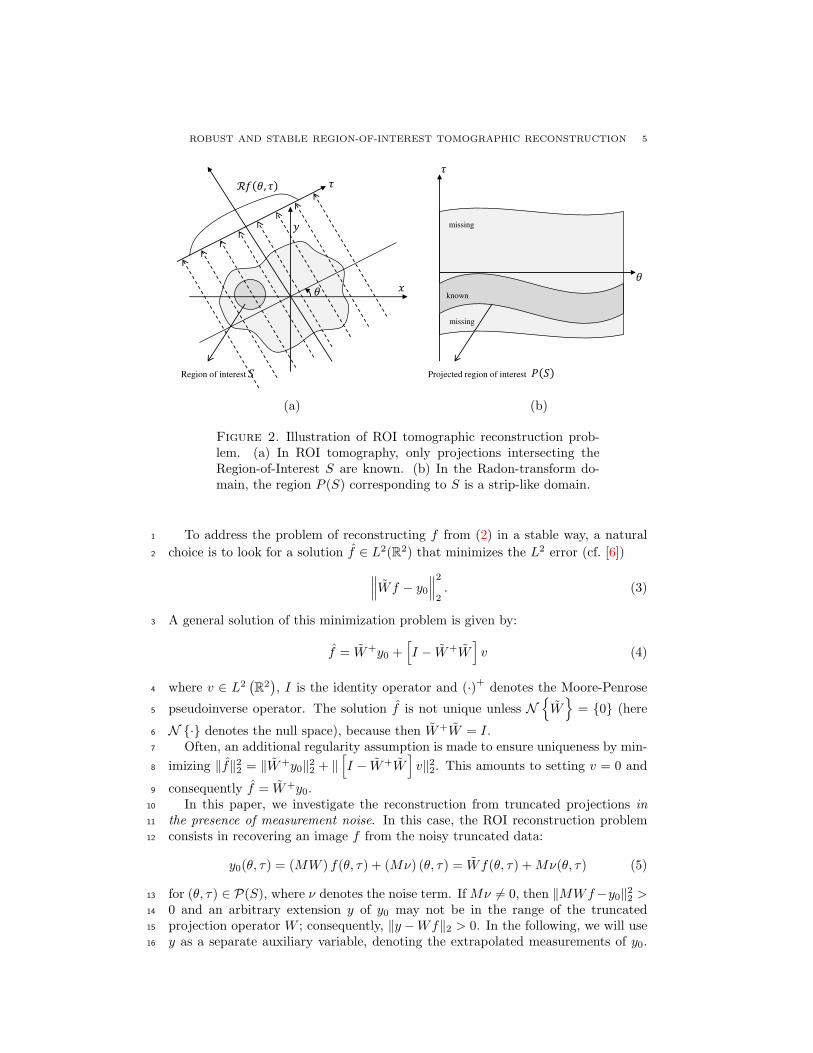
The goal of ROI tomography is to reconstruct a function from its projections12

within a subregion inside the field of view, while the rest of the image is ignored.13

That is – as shown in Fig. 2 – let us denote the ROI by S ⊂ R2 and define the14

subset of the tangent space associated with the rays that intersect the ROI S by:15

P(S) = {(θ, τ) ∈ T : ℓ(θ, τ) ∩ S = ∅} ;

corresponding to the set P(S), we define the mask function M on T by16

M(θ, τ) =

{1, (θ, τ) ∈ P(S)

0, otherwise;, (1)

we then formulate the ROI reconstruction problem as the problem of reconstructing17

f restricted to S from truncated projection data:18

y0(θ, τ) = Wf(θ, τ), for (θ, τ) ∈ P(S), (2)

where W is the composition of the mask function M and the projection operator19

W , i.e., W =MW . For simplicity, we assume in the following that the ROI S ⊂ R220

is a disk with center pROI ∈ R2 and radius RROI > 0. In this case, it is easy to21

derive that P(S) = {(θ, τ) ∈ T : |τ − pROI · eθ| < RROI}. The situation where S22

is a disk is natural in practical situations due to the circular trajectory of the x-ray23

source in many projection geometries.124

The inversion of W is ill-posed in general and the ill-posedness may be more25

severe (i.e., the condition number of the problem is higher) in the situation where26

the projection data are incomplete, as in the case given by (2). It is known that27

the so-called interior problem, where Wf(θ, τ) is given only for |τ | ≤ a and a is28

a positive constant, is not uniquely solvable in general [1]. A unique solution of29

the interior problem can be guaranteed if the density function f is assumed to be30

piece-wise polynomial in the interior region [27]. However, this assumes the ideal31

case of a noiseless acquisition and it leaves the problem of stability in the presence32

of noise open.33

1More general convex ROIs can be handled by calculating the minimal enclosing disk for this

ROI and reconstructing the image inside this disk.

ROBUST AND STABLE REGION-OF-INTEREST TOMOGRAPHIC RECONSTRUCTION 5

Region of interest Projected region of interest

known

missing

missing

(a) (b)

Figure 2. Illustration of ROI tomographic reconstruction prob-lem. (a) In ROI tomography, only projections intersecting theRegion-of-Interest S are known. (b) In the Radon-transform do-main, the region P (S) corresponding to S is a strip-like domain.

To address the problem of reconstructing f from (2) in a stable way, a natural1

choice is to look for a solution f ∈ L2(R2) that minimizes the L2 error (cf. [6])2 ∥∥∥Wf − y0

∥∥∥22. (3)

A general solution of this minimization problem is given by:3

f = W+y0 +[I − W+W

]v (4)

where v ∈ L2(R2), I is the identity operator and (·)+ denotes the Moore-Penrose4

pseudoinverse operator. The solution f is not unique unless N{W}

= {0} (here5

N {·} denotes the null space), because then W+W = I.6

Often, an additional regularity assumption is made to ensure uniqueness by min-7

imizing ∥f∥22 = ∥W+y0∥22 + ∥[I − W+W

]v∥22. This amounts to setting v = 0 and8

consequently f = W+y0.9

In this paper, we investigate the reconstruction from truncated projections in10

the presence of measurement noise. In this case, the ROI reconstruction problem11

consists in recovering an image f from the noisy truncated data:12

y0(θ, τ) = (MW ) f(θ, τ) + (Mν) (θ, τ) = Wf(θ, τ) +Mν(θ, τ) (5)

for (θ, τ) ∈ P(S), where ν denotes the noise term. IfMν = 0, then ∥MWf−y0∥22 >13

0 and an arbitrary extension y of y0 may not be in the range of the truncated14

projection operator W ; consequently, ∥y −Wf∥2 > 0. In the following, we will use15

y as a separate auxiliary variable, denoting the extrapolated measurements of y0.16

6 BART GOOSSENS AND DEMETRIO LABATE AND BERNHARD G BODMANN

Data fidelity Data consistency

Sparsity prior

Consistent

solutions

subspace

Fidelity

solutions

subspace

♯

Figure 3. Schematic illustration of the solution space for y, givena current estimate f , as intersection of the balls ∥My − y0∥2 ≤ α

and ∥y −Wf∥2 ≤ β, as well as solutions favored by the sparsityprior ∥y∥♯ (see Sec. 3). Data consistent solutions may have a non-zero data fidelity, while data fidelity solutions are in general notconsistent. We control the reconstruction error by combining fi-delity and consistency constraints with the additional sparsity as-sumption.

Setting tolerances, we formulate the two following constraints:1 {∥My − y0∥22 ≤ α (data fidelity)

∥y −Wf∥22 ≤ β (data consistency)(6)

where α is a data fidelity parameter (chosen in accordance with the noise level) and2

β is a data consistency parameter. By setting α = 0, a solution can be obtained that3

maximizes the data fidelity with respect to the measurement data, i.e., My = y0.4

Alternatively, setting β = 0 maximizes the data consistency of the solution, i.e.,5

y = Wf , so that the data fidelity constraint becomes ∥MWf − y0∥22 ≤ α. In6

the presence of noise, the parameters α and β generally cannot be set to zero7

simultaneously, as y0 may not be in the range of W .8

The selection of α and β allows us to trade off data fidelity versus data consis-9

tency, as illustrated in Fig. 3. By letting β > 0, data consistency errors are allowed10

and the solution space of the ROI problem is effectively enlarged, giving us better11

control on the denoising and extrapolation process of y0. Another advantage of our12

approach is that the leverage of data fidelity and data consistency constraints with13

the additional sparsity assumption enables us to establish performance guarantees14

in both the image and projection spaces. Our method will find a pair (y⋆, f⋆) where15

y⋆ is an approximate extension of y0 in (5) according to the data consistency con-16

straint and f⋆ is an approximate image reconstruction according to the data fidelity17

ROBUST AND STABLE REGION-OF-INTEREST TOMOGRAPHIC RECONSTRUCTION 7

constraint (6). Specifically, we will define an iterative algorithm based on convex1

optimization which is guaranteed to provide an approximation(y⋆, f⋆

)of (y⋆, f⋆)2

in a finite number of iterations and is within a predictable distance from the ideal3

noiseless solution of the ROI problem. We remark that, due to the non-injectivity4

of the truncated projection operator, data fidelity in the projection domain does not5

automatically imply a low reconstruction error in the image domain. To address6

this task, we introduce a compressed sensing framework to control data fidelity7

and reconstruction error by imposing an appropriate sparsity norm on both the8

projection data and the reconstructed image.9

3. Application of robust width to ROI CT reconstruction. The robust width10

property was originally introduced by Cahill and Mixon [15] as a geometric criterion11

that characterizes when the solution to a convex optimization problem provides an12

accurate approximate solution to an underdetermined, noise-affected linear system13

by assuming an additional structure of the solution space [16]. This property is14

related to the Restricted Isometry Property (RIP) that is widely used in compressed15

sensing, especially in conjunction with randomized measurements [22]. We adapt16

the result by Cahill and Mixon to our setting because it offers more flexibility than17

the usual assumptions in compressed sensing and leads to an algorithmic formulation18

of ROI reconstruction that includes a sparsity norm and a performance guarantee.19

We start by defining a notion of compressed sensing space that provides the20

appropriate approximation space for the solutions of the noisy ROI reconstruction21

problem.22

Definition 3.1. A compressed sensing (CS) space(H,A, ∥·∥♯

)with bound L con-23

sists of a Hilbert space H, a subset A ⊆ H and a norm or semi-norm ∥·∥♯ on H such24

that25

1. 0 ∈ A26

2. For every a ∈ A and z ∈ H, there exists a decomposition z = z1 + z2 such27

that28

∥a+ z1∥♯ = ∥a∥♯ + ∥z1∥♯with ∥z2∥♯ ≤ L∥z∥2.29

Remark 1. We have the upper bound30

L ≤ sup

{ ∥z∥♯∥z∥2

: z ∈ H \ {0}}. (7)

Remark 2. Suppose H is a Hilbert space, A ⊆ H, ∥·∥♯ is a norm such that31

1. 0 ∈ A32

2. For every a ∈ A and z ∈ H, there exists a decomposition z = z1 + z2 such33

that ⟨z1, z2⟩ = 0 and34

∥a+ z1∥♯ = ∥a∥♯ + ∥z1∥♯ , z2 ∈ A (8)

3. ∥a∥♯ ≤ L∥a∥2 for every a ∈ A35

Then(H,A, ∥·∥♯

)is a CS space with bound L.36

This follows from the observation that, since some z2 ∈ A is orthogonal to z1,37

then38

∥z2∥♯ ≤ L∥z2∥2 ≤ L√∥z1∥22 + ∥z2∥22 = L∥z∥2.

8 BART GOOSSENS AND DEMETRIO LABATE AND BERNHARD G BODMANN

Example 1. A standard example for a CS space is that of K sparse vectors [15].1

This structure is defined by choosing an orthonormal basis {ψj}∞j=1 in a Hilbert2

space H. The set A consists of vectors that are linear combinations of K basis3

vectors. The norm ∥·∥♯ is given by4

∥v∥♯ =∞∑j=1

|⟨v, ψj⟩| .

In this case, for any a ∈ A, which is the linear combination of {ψj}j∈J with |J | ≤5

K and z ∈ H, we can then choose the decomposition z2 =∑

j∈J ⟨z, ψj⟩ψj and6

z1 = z − z2. We then see that (8) holds and, since a is in the subspace spanned by7

{ψj}j∈J , by the equivalence of ℓ1 and ℓ2-norms for finite sequences, ∥a∥♯ ≤√K∥a∥2.8

Definition 3.2. A linear operator Φ : H → H satisfies the (ρ, η) robust width9

property (RWP) over B♯ ={x ∈ H : ∥x∥♯ ≤ 1

}if10

∥x∥2 < ρ ∥x∥♯for every x ∈ H s.t. ∥Φx∥2 ≤ η∥x∥2.11

The following theorem extends a result in [15]. In particular, we consider an12

approximate solution x⋆ of x⋆ such that ∥x⋆∥2 ≤ ∥x⋆∥2 + δ, in order to account for13

data fidelity, consistency and sparsity trade-offs (see further).14

Theorem 3.3. Let(H,A, ∥·∥♯

)be a CS space with bound L and Φ : H → H a15

linear operator satisfying the RWP over B♯, with ρ, η.16

For x♮ ∈ H, ϵ > 0, e ∈ H with ∥e∥2 ≤ ϵ, let x⋆ be a solution of17

∆♯,Φ,ϵ

(Φx♮ + e

)= argmin

x∈H∥x∥♯ subject to ∥Φx−

(Φx♮ + e

)∥2 ≤ ϵ.

Then for every x♮ ∈ H and a ∈ A, any approximate solution x⋆ of x⋆ such that18

∥x⋆∥2 ≤ ∥x⋆∥2 + δ, δ ≥ 0, satisfies19

∥x⋆ − x♮∥2 ≤ C1ϵ+ γρ∥∥x♮ − a

∥∥♯+

1

2γρδ,

provided that ρ ≤(

2γγ−2L

)−1

for some γ > 2 and with C1 = 2/η.20

Proof. See Appendix 6.1.21

We now adapt the CS reconstruction theorem (Theorem 3.3) to the CT ROI22

problem. We adopt the same notations as in Sec. 2 for the symbols W , M and y023

and we treat the projection data f and image space data y jointly.24

Theorem 3.4. Interior and exterior ROI reconstruction.25

Let H ={(y, f) : ∥ (y, f) ∥H = ∥f∥22 + ∥y∥22 <∞

}, A ⊂ H and26

Φ =

(I −WM 0

). (9)

Suppose(H,A, ∥·∥♯

)is a CS space and Φ : H → H satisfies the (ρ, η)-RWP over27

the ball B♯. Then, for every(y♮, f ♮

)∈ E = {(y, f) ∈ H : y =Wf, My = y0} , a28

solution (y⋆, f⋆), where29

(y⋆, f⋆) = arg min(y,f)∈H

∥(y, f)∥♯ s.t. ∥My−y0−ν∥2 ≤ αand∥y−Wf∥2 ≤ β (10)

ROBUST AND STABLE REGION-OF-INTEREST TOMOGRAPHIC RECONSTRUCTION 9

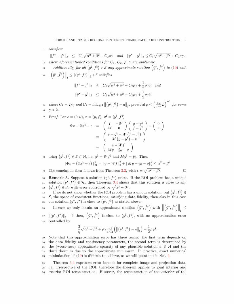
satisfies:1

∥f⋆ − f ♮∥2 ≤ C1

√α2 + β2 + C2ργ and ∥y⋆ − y♮∥2 ≤ C1

√α2 + β2 + C2ργ.

where aforementioned conditions for C1, C2, ρ, γ are applicable.2

Additionally, for all(y♮, f ♮

)∈ E any approximate solution

(y⋆, f⋆

)to (10) with3 ∥∥∥(y⋆, f⋆)∥∥∥

♯≤ ∥(y⋆, f⋆)∥♯ + δ satisfies4

∥f⋆ − f ♮∥2 ≤ C1

√α2 + β2 + C2ργ +

1

2ργδ and

∥y⋆ − y♮∥2 ≤ C1

√α2 + β2 + C2ργ +

1

2ργδ,

where C1 = 2/η and C2 = infa∈A∥∥(y♮, f ♮)− a

∥∥♯, provided ρ ≤

(2γγ−2L

)−1

for some5

γ > 2.6

Proof. Let e = (0, ν), x = (y, f), x♮ =(y♮, f ♮

)7

Φx− Φx♮ − e =

(I −WM 0

)(y − y♮

f − f ♮

)−(

0ν

)=

(y − y♮ −W

(f − f ♮

)M(y − y♮

)− ν

)=

(y −Wf

My − y0 − ν

)using

(y♮, f ♮

)∈ E ⊂ H, i.e. y♮ =Wf ♮ and My♮ = y0. Then8

∥Φx−(Φx♮ + e

)∥2H = ∥y −Wf∥22 + ∥My − y0 − ν∥22 ≤ α2 + β2

The conclusion then follows from Theorem 3.3, with ϵ =√α2 + β2.9

Remark 3. Suppose a solution (y⋆, f⋆) exists. If the ROI problem has a unique10

solution (y⋆, f⋆) ∈ H, then Theorem 3.4 shows that this solution is close to any11 (y♮, f ♮

)∈ A, with error controlled by

√α2 + β2.12

If we do not know whether the ROI problem has a unique solution, but(y♮, f ♮

)∈13

E , the space of consistent functions, satisfying data fidelity, then also in this case14

our solution (y⋆, f⋆) is close to(y♮, f ♮

)as stated above.15

In case we only obtain an approximate solution(y⋆, f⋆

)with

∥∥∥(y⋆, f⋆)∥∥∥♯≤16

∥(y⋆, f⋆)∥♯ + δ then,(y⋆, f⋆

)is close to

(y♮, f ♮

), with an approximation error17

controlled by18

2

η

√α2 + β2 + ργ inf

a∈A

(∥∥(y♮, f ♮)− a∥∥♯

)+

1

2ργδ.

Note that this approximation error has three terms: the first term depends on19

the data fidelity and consistency parameters, the second term is determined by20

the (worst-case) approximate sparsity of any plausible solution a ∈ A and the21

third therm is due to the approximate minimizer. In practice, exact numerical22

minimization of (10) is difficult to achieve, as we will point out in Sec. 4.23

Theorem 3.4 expresses error bounds for complete image and projection data,24

i.e., irrespective of the ROI, therefore the theorem applies to joint interior and25

exterior ROI reconstruction. However, the reconstruction of the exterior of the26

10 BART GOOSSENS AND DEMETRIO LABATE AND BERNHARD G BODMANN

Figure 4. Commutative diagram of the measurement operator Φand the restricted measurement operator Φ′ (see Theorem 3.5).The following relationship holds: PH′Φ = Φ′PH′ .

ROI is severely ill-posed: due to the nullspace of Φ, impractically strong sparseness1

assumptions are required to recover a stable reconstruction. Therefore, for a CS2

space with RWP (ρ, η), we may expect the error bounds C1 and C2 to be very3

large, especially when the radius of the ROI is small. To correct this situation, we4

restrict RWP within a linear subspace of the Hilbert space so that error bounds are5

obtained for linear projections onto a subspace spanned by a confined area such as6

the ROI, leading to interior -only ROI reconstruction. The next theorem gives the7

framework for constructing such projections.8

Theorem 3.5. Interior-only ROI reconstruction.9

Let H ={(y, f) : ∥ (y, f) ∥H = ∥f∥22 + ∥y∥22 <∞

}and10

Φ : H → H =

(I −WM 0

). (11)

Let PH′ =

(My

M

)be an orthogonal projection of H onto H′ ⊂ H, with

My defined such that MMy = M . Additionally, let PH′ =

(My

Mf

)be an

orthogonal projection of H onto H′ ⊂ H, with Mf and My intertwining operatorsw.r.t. W (i.e., WMf =MyW ) as shown in Fig. 4 and let Φ′ denote the restrictionof the measurement operator Φ to H′:

Φ′ : H′ → H′ = PH′ΦPH′ .

Suppose(H′,A, ∥·∥♯

), where A ⊂ H′, is a CS space and Φ′ satisfies the (ρ, η)-RWP11

over the ball B♯. Then, for every(y♮, f ♮

)∈ E = {(y, f) ∈ H : y =Wf, My = y0} ,12

a solution (y⋆, f⋆) ∈ H′,13

(y⋆, f⋆) = arg min(y,f)∈H′

∥(y, f)∥♯ s.t. ∥My−y0−ν∥2 ≤ αand∥My (y −Wf) ∥2 ≤ β

(12)satisfies:14

∥M(y⋆ − y♮

)∥2 ≤ ∥My

(y⋆ − y♮

)∥2 ≤ C1

√α2 + β2 + C2ργ and

∥Mf

(f⋆ − f ♮

)∥2 ≤ C1

√α2 + β2 + C2ργ (13)

where C1 = 2/η and C2 = infa∈A∥∥(y♮, f ♮)− a

∥∥♯, provided ρ ≤

(2γγ−2L

)−1

for some15

γ > 2.16

Proof. See Appendix 6.2.17

ROBUST AND STABLE REGION-OF-INTEREST TOMOGRAPHIC RECONSTRUCTION 11

Remark 4. Theorem 3.5 generalizes Theorem 3.4 to give performance guarantees1

for stable reconstruction within the ROI: for a CS space with (ρ, η)-RWP, the opera-2

torsMy andMf define a subspace H′ and determine the error bounds through (13).3

We have some flexibility in the choice of these operators. In particular, M =MMy4

implies that the orthogonal projection My is subject to ∥My∥2 ≤ ∥Myy∥2 ≤ ∥y∥2.5

For practical algorithms using fan-beam and cone-beam geometries, calculating6

Mf based on the relationship WMf =MyW is not trivial. The dependence of the7

solution method on Mf can be avoided by solving (12) as follows:8

(y⋆, f⋆) = arg min(y,f)∈H

∥(y, f)∥♯ s.t. ∥My − y0 − ν∥2 ≤ α and ∥My (y −Wf) ∥2 ≤ β,

(14)where the minimum is now taken over H instead of over H′. As we show in Exam-9

ple 2 below, we can always choose My such that ∥PH′ (y, f)∥♯ ≤ ∥(y, f)∥♯ . Corre-10

spondingly,11

min(y,f)∈H′

∥(y, f)∥♯ = min(y,f)∈H

∥PH′ (y, f)∥♯ ≤ min(y,f)∈H

∥(y, f)∥♯ .

Moreover, since H′ ⊂ H, we find that min(y,f)∈H′ ∥(y, f)∥♯ = min(y,f)∈H ∥(y, f)∥♯,i.e., (14) gives the exact minimizer for (12). In case that, due to the use of a numer-

ical method, we only obtain an approximate solution to (14) with∥∥∥(y⋆, f⋆)∥∥∥

♯≤

∥(y⋆, f⋆)∥♯ + δ where(y⋆, f⋆

)is the true solution of (14), we have again the ap-

proximation bounds following from Theorem 3.4:

∥Mf

(f⋆ − f ♮

)∥2 ≤ C1

√α2 + β2 + C2ργ +

1

2ργδ and

∥My

(y⋆ − y♮

)∥2 ≤ C1

√α2 + β2 + C2ργ +

1

2ργδ.

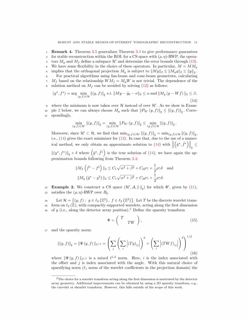
Example 2. We construct a CS space (H′,A, ∥·∥♯) for which Φ′, given by (11),12

satisfies the (ρ, η)-RWP over B♯.13

LetH ={(y, f) : y ∈ ℓ2

(Z2), f ∈ ℓ2

(Z2)}

. Let T be the discrete wavelet trans-14

form on ℓ2 (Z), with compactly supported wavelets, acting along the first dimension15

of y (i.e., along the detector array position).2 Define the sparsity transform16

Ψ =

(T

TW

), (15)

and the sparsity norm:17

∥(y, f)∥♯ = ∥Ψ(y, f) ∥ℓ1,2 =

∑j

(∑i

∣∣∣(Ty)ij∣∣∣)2

+

(∑i

∣∣∣(TWf)ij

∣∣∣)21/2

(16)where ∥Ψ(y, f) ∥ℓ1,2 is a mixed ℓ1,2 norm. Here, i is the index associated withthe offset and j is index associated with the angle. With this natural choice ofsparsifying norm (ℓ1 norm of the wavelet coefficients in the projection domain) the

2The choice for a wavelet transform acting along the first dimension is motivated by the detector

array geometry. Additional improvements can be obtained by using a 2D sparsity transform, e.g.,

the curvelet or shearlet transform. However, this falls outside of the scope of this work.

12 BART GOOSSENS AND DEMETRIO LABATE AND BERNHARD G BODMANN

transform basis functions can be associated with the ridgelets [28]. Additionally,define the solution space A as:

A ={(y, f) ∈ ℓ2

(Z2)| ∀j∈ Z :

((Ty):,j , (TWf):,j

)is a K-sparse vector

}where (·):,j denotes a vector slice. Then for (y, f) ∈ A, we have that

∥(y, f)∥♯ ≤ C√K ∥(y, f)∥2 ,

with C the upper frame bound of Ψ, or equivalently,1

supy∈A

∥(y, f)∥♯∥(y, f)∥2

≤ C√K. (17)

Next, we need to construct a projection operator My such that M = MMy. Forour practical algorithm (see Remark 4), we require that ∥PH′ (y, f)∥♯ ≤ ∥(y, f)∥♯ .In fact, this requirement can be accomplished by selecting a diagonal projectionoperator acting in the ridgelet domain forMy, i.e.,My = T ∗DyT withDy a diagonalprojection:

∥PH′ (y, f)∥♯ =(∥TMyy∥2ℓ1,2 + ∥TWMff∥2ℓ1,2

)1/2=(∥TMyy∥2ℓ1,2 + ∥TMyWf∥2ℓ1,2

)1/2=(∥DyTy∥2ℓ1,2 + ∥DyTWf∥2ℓ1,2

)1/2.

With this choice it follows that ∥DyTWf∥2ℓ1,2 ≤ ∥TWf∥2ℓ1,2 so that

∥PH′ (y, f)∥♯ ≤(∥Ty∥2ℓ1,2 + ∥TWf∥2ℓ1,2

)1/2= ∥(y, f)∥♯ .

To ensure that MT ∗DyT = My so that also ∥My∥2 ≤ ∥Myy∥2 = ∥DyTy∥2, one2

can design Dy as an indicator mask function that selects all wavelet and scaling3

functions that overlap with the ROI projection P(S).4

4. Sparsity-inducing ROI CT reconstruction algorithm (SIRA). In this5

section, we present an algorithm to solve the constrained optimization problem:6

(y, f) = arg min(y,f)∈H

∥(y, f)∥♯ s.t. ∥My − y0∥2 ≤ α and ∥y −Wf∥2 ≤ β.

By Theorem 3.4, a solution or approximate solution of this problem will yield an7

approximate solution of the ROI problem with a predictable error.8

Algorithm 1. For y, f , y(i), f (i), p and q ∈ H, let the Bregman divergence be (see9

[29]):10

Dp,qΨp

(y, f ; y(i), f (i)

)= ∥(y, f)∥♯ −

∥∥∥(y(i), f (i))∥∥∥♯−⟨p, y − y(i)

⟩−⟨q, f − f (i)

⟩.

With M and W as defined in Sec. 2, let the objective function H (y, f ; y0) be11

H (y, f ; y0) =β

2∥My − y0∥2 +

α

2∥y −Wf∥2 (18)

where α > 0 and β > 0. The Bregman iteration is then defined as follows:12

(y(i+1), f (i+1)) = arg min(y,f)

Dp(i),q(i)

Ψp

(y, f ; y(i), f (i)

)+H (y, f ; y0) ; (19)

p(i+1) = p(i) −∇yH(y(i+1), f (i+1); y0

);

q(i+1) = q(i) −∇fH(y(i+1), f (i+1); y0

).

ROBUST AND STABLE REGION-OF-INTEREST TOMOGRAPHIC RECONSTRUCTION 13

We have the following result.1

Theorem 4.1. Let δ > 0. Assume that there exists a point (y♮, f ♮) for which2

H(y♮, f ♮; y0

)< δ. Then, if H

(y(0), f (0); y0

)> δ, for any τ > 1 there exists i⋆ ∈ N3

such that H(yi⋆ , f i⋆ ; y0

)≤ τ δ. More specifically4

H(yi, f i; y0

)≤ δ +

D0

i

with D0 = Dp0,q0Ψp

(y♮, f ♮; y(0), f (0)

)≥ 0.5

To prove this result, we need the following observation showing that under the6

Bregman iteration, the Bregman divergence and the objective function are both7

non-increasing. The following result is adapted from [29, Proposition 3.2].8

Proposition 1. Let δ > 0. Assume that, for a given (y♮, f ♮), we have that9

H(y♮, f ♮; y0

)< δ. Then, as long as H

(y(i), f (i); y0

)> δ, the Bregman divergence10

between (y♮, f ♮) and (y(i), f (i)) is non increasing, i.e.,11

Dpi,qiΨp

(y♮, f ♮; y(i), f (i)

)≤ D

pi−1,qi−1

Ψp

(y♮, f ♮; y(i−1), f (i−1)

)(20)

and the objective function H, given by (18), is also non increasing,12

H(y(i), f (i); y0

)≤ H

(y(i−1), f (i−1); y0

). (21)

Proof. See Appendix 6.3.13

For implementation purposes, it is convenient to replace the Bregman iteration14

with the following Bregman iteration variant [30]:15

Algorithm 2.

ϵ(i+1) = y(i) −Wf (i)

y(i+1)0 = y

(i)0 +

(My(i) − y0

)(y(i+1), f (i+1)) = arg min

(y,f)∥(y, f)∥♯ +

β

2∥My − y

(i+1)0 ∥2

+α

2∥y −Wf − ϵ(i+1)∥2 (22)

The following Proposition shows that the minimization in equations (19) and16

(22) are equivalent.17

Proposition 2. The minimum values obtained in each iteration step of Algo-18

rithm 2, are identical to the corresponding values for Algorithm 1:19

min(y,f)

∥(y, f)∥♯ +β

2∥My − y

(i+1)0 ∥2 + α

2∥y −Wf − ϵ(i+1)∥2

= min(y,f)

Dp(i),q(i)

Ψp

(y, f ; y(i), f (i)

)+H (y, f ; y0) .

Proof. See Appendix 6.4.20

Remark 5. For the objective function H (y, f ; y0) as defined in (18), we have that21

from H(y(i⋆), f (i⋆); y0

)≤ τ δ it follows that22

β∥My(i⋆) − y0∥2 ≤ 2τ δ and α∥y(i⋆) −Wf (i⋆)∥2 ≤ 2τ δ.

14 BART GOOSSENS AND DEMETRIO LABATE AND BERNHARD G BODMANN

Therefore, if α > 0 and β > 0, if we choose δ = αβ/ (2τ) then we have that1

∥My(i⋆)−y0∥2 ≤ α and ∥y(i⋆)−Wf (i⋆)∥2 ≤ β. This way, we obtain the approximate2

solution(y⋆, f⋆

)=(y(i⋆), f (i⋆)

)for (10).3

The limiting cases α = 0 or β = 0 can also be solved using the above algorithm,4

but the function H (y, f ; y0) needs to be modified.5

In case β = 0, we minimize H (y, f ; y0) = 12∥My − y0∥2 while imposing data6

consistency through the constraint y =Wf . Similarly, Theorem 4.1 will imply that7

∥My(i⋆) − y0∥2 ≤ 2τ δ = α.8

In case α = 0, we minimize H (y, f ; y0) = 12∥y − Wf∥2 while enforcing strict9

data fidelity, i.e., My = y0. Then Theorem 4.1 will imply that ∥y(i⋆) −Wf (i⋆)∥2 ≤10

2τ δ = β.11

The character of the reconstruction obtained in the limiting cases is illustrated12

in Fig. 3.13

The following proposition outlines a practical approach to select the data fidelity14

and consistency parameters based on the measured projection data y0. When α and15

β are within suitable ranges, it can be guaranteed that the conditions of Proposi-16

tion 1 are satisfied.17

Proposition 3. Choose δ as in Remark 5. With the initialization y(0) = My018

and f (0) = W+y(0), for α > 0, the initial conditions for Proposition 1 (namely,19

H(y(0), f (0); y0

)> δ and ∃

(y♮, f ♮

): H

(y♮, f ♮; y0

)< δ) are satisfied if at least one20

of the following conditions holds:21

τ(∥(I − WW+

)y0∥2 − ∥

(I −WW+

)y0∥2

)2< β ≤ τ∥

(I −WW+

)y0∥22

τ∥(I − WW+

)y0∥22 < α

Proof. See Appendix 6.5.22

Similarly, for α = 0, it can be shown that23

τ∥(I − WW+

)y0∥22 < β ≤ τ∥

(I −WW+

)y0∥22.

5. Results and discussion. In this section, we evaluate the ROI reconstruction24

performance of the convex optimization algorithm SIRA from Sec. 4 as a function of25

data fidelity and consistency parameters as well as the size of the ROI radius. The26

numerical tests were run on an Intel Core I7-5930K CPU with NVIDIA Geforce RTX27

2080 GPU, with 8 GB RAM GPU memory. The algorithms were implemented in28

Quasar [31], which provides a heterogeneous GPU/CPU programming environment29

on top of CUDA and OpenMP.30

5.1. ROI reconstruction results. The X-O CT system (Gamma Medica-Ideas,31

Northridge, California, USA) was used to obtain in vivo preclinical data. The tube32

current is determined automatically during calibration to ensure that the dynamic33

range of the detector is optimally used. For a 50 µm spot size at 70 kVp, this34

amounts to 145 µA tube current. Fan-beam data were generated by retaining35

only the central detector row. Two contrast-enhanced mice were scanned in-vivo,36

resulting in two data sets (see Fig. 5):37

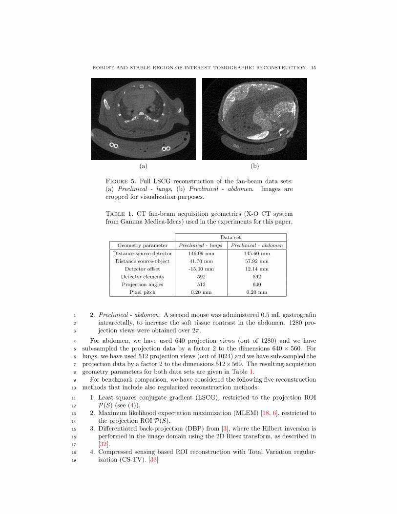
1. Preclinical - lungs: A first mouse was injected with a lipid-bound iodine-based38

contrast agent (Fenestra VC, ART, Canada), to increase the vascular contrast.39

2048 projection views were obtained over 2π.40

ROBUST AND STABLE REGION-OF-INTEREST TOMOGRAPHIC RECONSTRUCTION 15

(a) (b)

Figure 5. Full LSCG reconstruction of the fan-beam data sets:(a) Preclinical - lungs, (b) Preclinical - abdomen. Images arecropped for visualization purposes.

Table 1. CT fan-beam acquisition geometries (X-O CT systemfrom Gamma Medica-Ideas) used in the experiments for this paper.

Data set

Geometry parameter Preclinical - lungs Preclinical - abdomen

Distance source-detector 146.09 mm 145.60 mm

Distance source-object 41.70 mm 57.92 mm

Detector offset -15.00 mm 12.14 mm

Detector elements 592 592

Projection angles 512 640

Pixel pitch 0.20 mm 0.20 mm

2. Preclinical - abdomen: A second mouse was administered 0.5 mL gastrografin1

intrarectally, to increase the soft tissue contrast in the abdomen. 1280 pro-2

jection views were obtained over 2π.3

For abdomen, we have used 640 projection views (out of 1280) and we have4

sub-sampled the projection data by a factor 2 to the dimensions 640 × 560. For5

lungs, we have used 512 projection views (out of 1024) and we have sub-sampled the6

projection data by a factor 2 to the dimensions 512×560. The resulting acquisition7

geometry parameters for both data sets are given in Table 1.8

For benchmark comparison, we have considered the following five reconstruction9

methods that include also regularized reconstruction methods:10

1. Least-squares conjugate gradient (LSCG), restricted to the projection ROI11

P(S) (see (4)).12

2. Maximum likelihood expectation maximization (MLEM) [18, 6], restricted to13

the projection ROI P(S).14

3. Differentiated back-projection (DBP) from [3], where the Hilbert inversion is15

performed in the image domain using the 2D Riesz transform, as described in16

[32].17

4. Compressed sensing based ROI reconstruction with Total Variation regular-18

ization (CS-TV). [33]19

16 BART GOOSSENS AND DEMETRIO LABATE AND BERNHARD G BODMANN

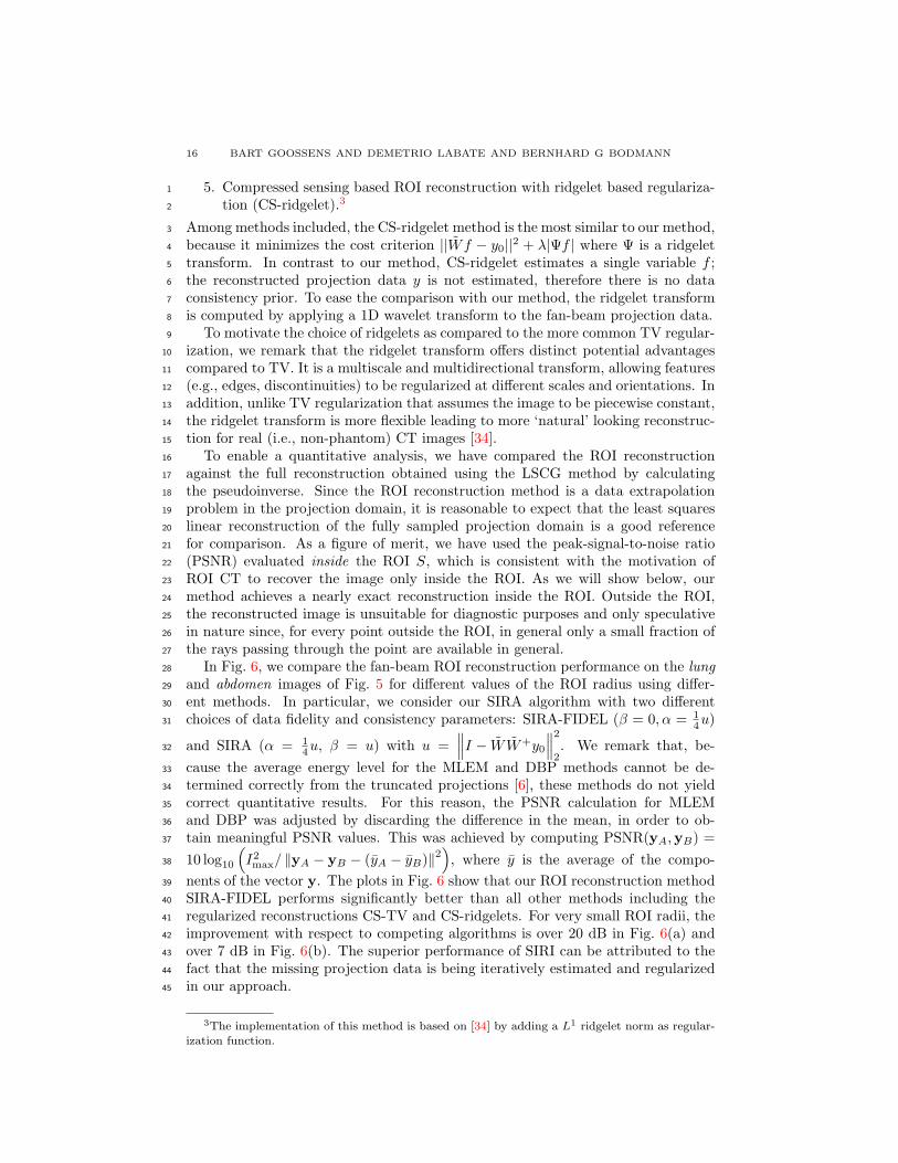
5. Compressed sensing based ROI reconstruction with ridgelet based regulariza-1

tion (CS-ridgelet).32

Among methods included, the CS-ridgelet method is the most similar to our method,3

because it minimizes the cost criterion ||Wf − y0||2 + λ|Ψf | where Ψ is a ridgelet4

transform. In contrast to our method, CS-ridgelet estimates a single variable f ;5

the reconstructed projection data y is not estimated, therefore there is no data6

consistency prior. To ease the comparison with our method, the ridgelet transform7

is computed by applying a 1D wavelet transform to the fan-beam projection data.8

To motivate the choice of ridgelets as compared to the more common TV regular-9

ization, we remark that the ridgelet transform offers distinct potential advantages10

compared to TV. It is a multiscale and multidirectional transform, allowing features11

(e.g., edges, discontinuities) to be regularized at different scales and orientations. In12

addition, unlike TV regularization that assumes the image to be piecewise constant,13

the ridgelet transform is more flexible leading to more ‘natural’ looking reconstruc-14

tion for real (i.e., non-phantom) CT images [34].15

To enable a quantitative analysis, we have compared the ROI reconstruction16

against the full reconstruction obtained using the LSCG method by calculating17

the pseudoinverse. Since the ROI reconstruction method is a data extrapolation18

problem in the projection domain, it is reasonable to expect that the least squares19

linear reconstruction of the fully sampled projection domain is a good reference20

for comparison. As a figure of merit, we have used the peak-signal-to-noise ratio21

(PSNR) evaluated inside the ROI S, which is consistent with the motivation of22

ROI CT to recover the image only inside the ROI. As we will show below, our23

method achieves a nearly exact reconstruction inside the ROI. Outside the ROI,24

the reconstructed image is unsuitable for diagnostic purposes and only speculative25

in nature since, for every point outside the ROI, in general only a small fraction of26

the rays passing through the point are available in general.27

In Fig. 6, we compare the fan-beam ROI reconstruction performance on the lung28

and abdomen images of Fig. 5 for different values of the ROI radius using differ-29

ent methods. In particular, we consider our SIRA algorithm with two different30

choices of data fidelity and consistency parameters: SIRA-FIDEL (β = 0, α = 14u)31

and SIRA (α = 14u, β = u) with u =

∥∥∥I − WW+y0

∥∥∥22. We remark that, be-32

cause the average energy level for the MLEM and DBP methods cannot be de-33

termined correctly from the truncated projections [6], these methods do not yield34

correct quantitative results. For this reason, the PSNR calculation for MLEM35

and DBP was adjusted by discarding the difference in the mean, in order to ob-36

tain meaningful PSNR values. This was achieved by computing PSNR(yA,yB) =37

10 log10

(I2max/ ∥yA − yB − (yA − yB)∥2

), where y is the average of the compo-38

nents of the vector y. The plots in Fig. 6 show that our ROI reconstruction method39

SIRA-FIDEL performs significantly better than all other methods including the40

regularized reconstructions CS-TV and CS-ridgelets. For very small ROI radii, the41

improvement with respect to competing algorithms is over 20 dB in Fig. 6(a) and42

over 7 dB in Fig. 6(b). The superior performance of SIRI can be attributed to the43

fact that the missing projection data is being iteratively estimated and regularized44

in our approach.45

3The implementation of this method is based on [34] by adding a L1 ridgelet norm as regular-

ization function.

ROBUST AND STABLE REGION-OF-INTEREST TOMOGRAPHIC RECONSTRUCTION 17

ROI Radius R

PS

NR

[dB

]

0 20 40 60 80 100 120 1404

8

12

16

20

24

28

32

36

40

SIRA-FIDELSIRACS-TVCS-ridgeletDBPMLEMLSCG

(a) Preclinical - lungs

ROI Radius R

PS

NR

[dB

]

0 20 40 60 80 100 120 1408

12

16

20

24

28

32

36

40

44

SIRA-FIDELSIRACS-TVCS-ridgeletDBPMLEMLSCG

(b) Preclinical - abdomen

Figure 6. PSNR results for 2D fan-beam ROI reconstruction withincreasing radius using (a) lungs and (b) adbomen. The PSNR iscalculated inside the ROI.

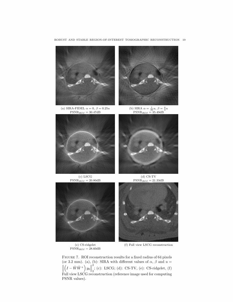
In Fig. 7, we show the visual comparison for the fan-beam ROI reconstruction1

of the lung and abdomen images in Fig. 5 using different methods. The parameters2

(α = 130u, β = 4

3u) in Fig. 5(b) correspond to the maximal PSNR performance in3

the range 0 ≤ β ≤ u and 0 ≤ α ≤ u (in steps of 0.1 for both β and α).4

A visual comparison to Fig. 7(f) yields that the SIRA algorithm reconstructs5

the interior of the ROI more accurately than competing method including CS-6

ridgelet, the next best method, resulting in a significantly higher PSNR. We also7

find that, by relaxing the data consistency constraint in (Fig. 5(b)), the PSNR8

performance can be improved compared to the data fidelity solution (Fig. 5(a)).9

We note that additional improvements are possible: for example, by using curvelets10

18 BART GOOSSENS AND DEMETRIO LABATE AND BERNHARD G BODMANN

[24] or shearlets [35] for regularization, rather than ridgelets. However this falls1

outside the scope of the paper and will be investigated elsewhere.2

Finally, we compare the visual performance of SIRA and LSCG for an increasing3

ROI radius. The results in Fig. 8 show that, even for a very small ROI radius of4

1.2 mm, the reconstruction quality for SIRA remains very satisfactory, while LSCG5

causes a cupping artifact at the boundary of the ROI. In terms of PSNR, SIRA6

offers significant performance gains compared to LSCG. Since LSCG optimizes over7

all data consistent solutions (y = Wf), this result again suggests that relaxing8

the consistency requirement in the right setting, can enhance the reconstruction9

performance in the image domain.10

Due to the robust width assumption (see Sec. 3), our theoretical framework offers11

performance guarantees for the image domain reconstruction performance. Even12

though Theorem 3.4 gives performance guarantees for both within the ROI (interior13

reconstruction) and outside of the ROI (exterior reconstruction), the latter task is14

significantly more difficult and requires additional prior knowledge. An interesting15

avenue for future research is the inclusion of priors based on e.g., combined sparsity16

models (ridgelets, wavelets and shearlets) and deep learning models (e.g., based on17

U-Net [11] and ResNet architectures).18

6. Conclusion. We have introduced a novel framework for ROI CT reconstruction19

from noisy projection data. To deal with the presence of noise, our method relaxes20

the data fidelity and consistency conditions. Based on a robust width assumption21

that guarantees stable solution of the ROI CT reconstruction problem under appro-22

priate sparsity norms on the data, we have established performance bounds in both23

the image and projection domains. Using this framework, we introduced a ROI CT24

reconstruction algorithm called sparsity-induced iterative reconstruction algorithm25

(SIRA), that reaches an approximately sparse solution in a finite number of steps26

while satisfying predetermined fidelity and consistency tolerances. Our experimen-27

tal results using fan-beam acquisition geometry suggest that the ROI reconstruction28

performance depends on the ROI radius. Visual and quantitative results confirm29

that our algorithm achieves very accurate reconstruction for relatively small ROI30

radii and demonstrate that our algorithm is very competitive against both conven-31

tional and state-of-the-art reconstruction methods.32

REFERENCES33

[1] F. Natterer, The Mathematics of Computerized Tomography. SIAM: Society for Industrial34

and Applied Mathematics, 2001.35

[2] R. Clackdoyle and M. Defrise, “Tomographic Reconstruction in the 21st century. Region-of-36

interest reconstruction from incomplete data,” IEEE Signal Processing, vol. 60, pp. 60–80,37

2010.38

[3] F. Noo, R. Clackdoyle, and J. Pack, “A two-step Hilbert transform method for 2D image39

reconstruction,” Phys. Med. Biol., vol. 49, pp. 3903–3923, 2004.40

[4] H. Kudo, M. Courdurier, F. Noo, and M. Defrise, “Tiny a priori knowledge solves the interior41

problem in computed tomography,” Phys. Med. Biol., vol. 53, pp. 2207–3923, 2008.42

[5] R. Clackdoyle, F. Noo, J. Guo, and J. Roberts, “Quantitative reconstruction from truncated43

projections in classical tomography,” IEEE Trans Nuclear Science, vol. 51, no. 5, pp. 2570–44

2578, 2004.45

[6] B. Zhang and G. L. Zeng, “Two-dimensional iterative region-of-interest (ROI) reconstruction46

from truncated projection data,” Med. Phys., vol. 3, pp. 935–944, 2007.47

[7] G. Zeng and G. Gullberg, “Exact iterative reconstruction for the interior problem,” Physics48

of Medical Biology, vol. 54, no. 19, pp. 5805–5814, 2009.49

ROBUST AND STABLE REGION-OF-INTEREST TOMOGRAPHIC RECONSTRUCTION 19

(a) SIRA-FIDEL α = 0, β = 0.25u (b) SIRA α = 130

u, β = 43u

PSNRROI = 30.47dB PSNRROI = 35.49dB

(c) LSCG (d) CS-TV

PSNRROI = 20.80dB PSNRROI = 21.33dB

(e) CS-ridgelet (f) Full view LSCG reconstructionPSNRROI = 28.60dB

Figure 7. ROI reconstruction results for a fixed radius of 64 pixels(or 3.2 mm). (a), (b): SIRA with different values of α, β and u =∥∥∥(I − WW+

)y0

∥∥∥22; (c): LSCG; (d): CS-TV, (e): CS-ridgelet, (f)

Full view LSCG reconstruction (reference image used for computingPSNR values).

20 BART GOOSSENS AND DEMETRIO LABATE AND BERNHARD G BODMANN

RROI = 24 (1.2 mm) RROI = 48 (2.4 mm) RROI = 96 (4.8 mm)

(a) PSNRROI = 25.38dB (b) PSNRROI = 28.38dB (c) PSNRROI = 35.66dB

(d) PSNRROI = 14.39dB (e) PSNRROI = 21.27dB (f) PSNRROI = 30.38dB

Figure 8. (a)-(c): Reconstruction results for different ROIradii using SIRA with fixed parameters α = 0, β =

0.25∥∥∥(I − WW+

)y0

∥∥∥22. (d)-(f): Reconstruction results using

LSCG for same ROI radii.

[8] Q. Xu, X. Mou, G. Wang, J. Sieren, E. Hoffman, and H. Yu, “Statistical interior tomography,”1

IEEE Transactions on Medical Imaging, vol. 30, no. 5, pp. 1116–1128, 2011.2

[9] X. Jin, A. Katsevich, H. Yu, G. Wang, L. Li, and Z. Chen, “Interior tomography with contin-3

uous singular value decomposition,” IEEE Transactions on Medical Imaging, vol. 31, no. 11,4

pp. 2108–2119, 2012.5

[10] H. Yu, Y. Ye, and G. Wang, “Interior reconstruction using the truncated Hilbert transform6

via singular value decomposition,” J. Xray Sci. Technol., vol. 16, no. 4, pp. 243–251, 2008.7

[11] T. A. Bubba, G. Kutyniok, M. Lassas, M. Maerz, W. Samek, S. Siltanen, and V. Srinivasan,8

“Learning the invisible: A hybrid deep learning-shearlet framework for limited angle computed9

tomography,” Inverse Problems, vol. 35, no. 6, p. 064002, 2019.10

[12] Y. Han, J. Gu, and J. C. Ye, “Deep learning interior tomography for region-of-interest recon-11

struction,” arXiv preprint arXiv:1712.10248, 2017.12

[13] T. Wurfl, F. C. Ghesu, V. Christlein, and A. Maier, “Deep learning computed tomography,”13

in International conference on medical image computing and computer-assisted intervention.14

Springer, 2016, pp. 432–440.15

[14] Y. Han and J. C. Ye, “Framing u-net via deep convolutional framelets: Application to sparse-16

view ct,” IEEE transactions on medical imaging, vol. 37, no. 6, pp. 1418–1429, 2018.17

[15] J. Cahill and D. G. Mixon, “Robust width: A characterization of uniformly stable and robust18

compressed sensing,” arXiv:1408.4409.19

[16] J. Cahill, X. Chen, and R. Wang, “The gap between the null space property and the restricted20

isometry property,” Linear Algebra and its Applications, vol. 501, pp. 363–375, 2016.21

[17] G. T. Herman and A. Lent, “Iterative reconstruction algorithms,” Computers in Biology and22

Medicine, vol. 6, no. 4, pp. 273–294, Oct. 1976.23

[18] L. A. Shepp and Y. Vardi, “Maximum likelihood reconstruction for emission tomography.”24

IEEE Trans Med Imaging, vol. 1, no. 2, pp. 113–122, 1982.25

ROBUST AND STABLE REGION-OF-INTEREST TOMOGRAPHIC RECONSTRUCTION 21

[19] M. R. Hestenes and E. Stiefel, “Methods of Conjugate Gradients for Solving Linear Systems,”1

Journal of Research of the National Bureau of Standards, vol. 6, pp. 409–436, 1952.2

[20] S. Kawata and O. Nalcioglu, “Constrained iterative reconstruction by the conjugate gradient3

method,” IEEE Transactions on Medical Imaging, vol. 4, no. 2, pp. 65–71, 1985.4

[21] D. F. Yu, J. A. Fessler, and E. P. Ficaro, “Maximum-likelihood transmission image reconstruc-5

tion for overlapping transmission beams,” IEEE Transactions on Medical Imaging, vol. 19,6

no. 11, pp. 1094–1105, 2000.7

[22] S. Foucart and H. Rauhut, A Mathematical Introduction to Compressive Sensing. Birkhauser8

Basel, 2013.9

[23] C. Metzler, A. Maleki, and R. Baraniuk, “From denoising to compressed sensing,” IEEE10

Transactions on Information Theory, vol. 62, no. 9, pp. 5117–5144, 2016.11

[24] E. Candes and D. Donoho, “Recovering edges in ill-posed inverse problems: Optimality of12

curvelet frames,” Annals of statistics, pp. 784–842, 2002.13

[25] F. Colonna, G. Easley, K. Guo, and D. Labate, “Radon transform inversion using the shearlet14

representation,” Appl. Comput. Harmon. Anal., vol. 29, no. 2, pp. 232–250, 2000.15

[26] F. Natterer and F. Wubbeling, Mathematical Methods in Image Reconstruction. SIAM:16

Society for Industrial and Applied Mathematics, 2001.17

[27] E. Klann, E. Quinto, and R. Ramlau, “Wavelet Methods for a Weighted Sparsity Penalty for18

Region of Interest Tomography,” Inverse Problems, vol. 31, no. 2, p. 025001, 2015.19

[28] E. Candes and D. Donoho, “Ridgelets: a key to higher-dimensional intermittency?” Phil.20

Trans. R. Soc. Lond. A., vol. 357, pp. 2495–2509, 1999.21

[29] S. Osher, M. Burger, D. Goldfarb, J. Xu, and W. Yin, “An Interative Regularization Method22

for Total Variation-Based Image Restoration,” SIAM Multiscale Modeling and Simulation,23

vol. 4, no. 2, pp. 460–489, 2005.24

[30] W. Yin, S. Osher, D. Goldfarb, and J. Darbon, “Bregman Iterative Algorithms for l1-25

Minimization with Applications to Compressed Sensing,” SIAM Journal on Imaging Sciences,26

vol. 1, no. 1, pp. 143–168, 2008.27

[31] B. Goossens, “Dataflow management, dynamic load balancing, and concurrent processing28

for real-time embedded vision applications using quasar,” International Journal of Circuit29

Theory and Applications, vol. 46, no. 9, pp. 1733–1755, 2018.30

[32] M. Felsberg, “A Novel Two-Step Method for CT Reconstruction,” in Bildverarbeitung fur die31

Medizin. Springer, 2008, pp. 303–307.32

[33] H. Kudo, T. Suzuki, and E. A. Rashed, “Image reconstruction for sparse-view CT and interior33

CT - introduction to compressed sensing and differentiated backprojection,” Quantitative34

imaging in medicine and surgery, vol. 3, no. 3, p. 147, 2013.35

[34] B. Vandeghinste, B. Goossens, R. Van Holen, C. Vanhove, A. Pizurica, S. Vandenberghe, and36

S. Staelens, “Iterative CT reconstruction using shearlet-based regularization,” IEEE Trans.37

Nuclear Science, vol. 60, no. 5, pp. p. 3305–3317, Oct. 2013.38

[35] G. Easley, D. Labate, and W. Lim, “Sparse Directional Image Representations using the39

Discrete Shearlet Transform,” Applied and Computational Harmonic Analysis, vol. 25, pp.40

25–46, 2008.41

Appendix.42

6.1. Proof of Theorem 3.3. Our proof of Theorem 3.3 is adapted from [15].43

Proof. Pick a ∈ A and write x⋆ − x♮ = z1 + z2 so that44

∥a+ z1∥♯ = ∥a∥♯ + ∥z1∥♯ and ∥z2∥♯ ≤ L∥x⋆ − x♮∥2Now45

∥a∥♯ +∥∥x♮ − a

∥∥♯

≥∥∥x♮∥∥

♯≥ ∥x⋆∥♯ ≥ ∥x⋆∥♯ − δ

=∥∥x♮ + (x⋆ − x♮

)∥∥♯− δ

=∥∥x♮ + z1 + z2

∥∥♯− δ

=∥∥a+ (x♮ − a

)+ z1 + z2

∥∥♯− δ

≥ ∥a+ z1∥♯ −∥∥(x♮ − a

)+ z2

∥∥♯− δ

22 BART GOOSSENS AND DEMETRIO LABATE AND BERNHARD G BODMANN

≥ ∥a+ z1∥♯ −∥∥x♮ − a

∥∥♯− ∥z2∥♯ − δ

= ∥a∥♯ + ∥z1∥♯ −∥∥x♮ − a

∥∥♯− ∥z2∥♯ − δ

Hence:1

∥z1∥♯ ≤ 2∥∥x♮ − a

∥∥♯+ ∥z2∥♯ + δ

Now2 ∥∥x⋆ − x♮∥∥♯≤ ∥z1∥♯ + ∥z2∥♯ ≤ 2

∥∥x♮ − a∥∥♯+ 2 ∥z2∥♯ + δ (23)

Assume ∥x⋆ − x♮∥2 > C1ϵ since otherwise we are done. In this case3

∥Φx⋆ − Φx♮∥2 ≤ ∥Φx⋆ −(Φx♮ + e

)∥2 + ∥e∥2 ≤ 2ϵ <

2

C1∥x⋆ − x♮∥2 = η∥x⋆ − x♮∥2

By RWP,4

∥x⋆ − x♮∥2 ≤ ρ∥∥x⋆ − x♮

∥∥♯

Recall that5

∥z2∥♯ ≤ L∥x⋆ − x♮∥2 ≤ ρL∥∥x⋆ − x♮

∥∥♯

Into (23):6 ∥∥x⋆ − x♮∥∥♯≤ 2

∥∥x♮ − a∥∥♯+ 2ρL

∥∥x⋆ − x♮∥∥♯+ δ

7

⇒∥∥x⋆ − x♮

∥∥♯≤ 2

1− 2ρL

∥∥x♮ − a∥∥♯+

1

1− 2ρLδ

⇒ ∥x⋆ − x♮∥2 ≤ ρ∥∥x⋆ − x♮

∥∥♯≤ 2ρ

1− 2ρL

∥∥x♮ − a∥∥♯+

1ρ

1− 2ρLδ + C1ϵ

= ργ∥∥x♮ − a

∥∥♯+

1

2ργδ + C1ϵ

provided ρ ≤(

2γγ−2L

)−1

for some γ > 2.8

6.2. Proof of Theorem 3.5.9

Proof. Let e = (0, ν) ∈ H, x = (y, f) ∈ H, x♮ =(y♮, f ♮

)∈ E . Equation (11) yields10

that11

Φ′ = PH′ΦPH′ =

(My −MyWMf

M 0

),

where we used that MMy = M . Taking into account that WMf = MyW, we find12

that13

Φ′ =

(My −MyWM 0

)so that also

Φ′x−(Φ′x♮ + e

)=

(My (y −Wf)−My

(y♮ −Wf ♮

)M(y − y♮)− ν

)=

(My (y −Wf)My − y0 − ν

),

using(y♮, f ♮

)∈ E ⊂ H, i.e. y♮ = Wf ♮ and My♮ = y0. Calculating the squared

norm, we have:

∥Φ′x−(Φ′x♮ + e

)∥22 = ∥My (y −Wf) ∥22 + ∥My − y0 − ν∥22 ≤ α2 + β2.

Then, due to the fact that(H′,A, ∥·∥♯

)is a CS space, and because of the (ρ, η)-

RWP of Φ′ over the ball B♯, we can apply again Theorem 3.3, with ϵ =√α2 + β2,

ROBUST AND STABLE REGION-OF-INTEREST TOMOGRAPHIC RECONSTRUCTION 23

for any x♮ ∈ E ∩ H′. In particular, for any x♮ /∈ H \ E for and for (y⋆, f⋆) ∈ H′

minimizing (12), we have that

∥PH′(x⋆ − x♮

)∥H = ∥My

(y⋆ − y♮

)∥22 + ∥Mf

(f⋆ − f ♮

)∥22 ≤ C1

√α2 + β2 + C2ργ.

The conclusion then follows noting that ∥My∥2 = ∥MMyy∥2 ≤ ∥Myy∥2 such that1

∥M(y⋆ − y♮

)∥2 ≤ ∥My

(y⋆ − y♮

)∥2.2

6.3. Proof of Theorem 4.1.3

Proof. Bregman divergences are positive such that:4

H(y(i), f (i); y0

)≤ Q(i)

(y(i), f (i)

)where5

Q(i)(y(i), f (i)

)= H

(y(i), f (i); y0

)+D

pi−1,qi−1

Ψp

(y♮, f ♮; y(i−1), f (i−1)

).

Due to the minimization in every iteration, we have that6

Q(i)(y(i), f (i)

)≤ Q(i)

(y(i−1), f (i−1)

).

Knowing that Q(i)(y(i−1), f (i−1)

)= H

(y(i−1), f (i−1); y0

)we find that:7

H(y(i), f (i); y0

)≤ H

(y(i−1), f (i−1); y0

).

This proves (21).8

To prove (20), let (y, f) be such that ∥(y, f)∥♯ < ∞. We have the following9

known identity (cf. [29]):10

Dpi,qiΨp

(y, f ; y(i), f (i)

)−D

pi−1,qi−1

Ψp

(y, f ; y(i−1), f (i−1)

)+D

pi−1,qi−1

Ψp

(y(i), f (i); y(i−1), f (i−1)

)=⟨y(i) − y, pi − pi−1

⟩+⟨f (i) − f, qi − qi−1

⟩=⟨y(i) − y,−∇yH

(y(i), f (i); y0

)⟩+⟨f (i) − f,−∇fH

(y(i), f (i); y0

)⟩.

By the convexity of H and the comparison with its linearization, we then conclude11

that for every (y, f)12

Dpi,qiΨp

(y, f ; y(i), f (i)

)−D

pi−1,qi−1

Ψp

(y, f ; y(i−1), f (i−1)

)+D

pi−1,qi−1

Ψp

(y(i), f (i); y(i−1), f (i−1)

)≤ H (y, f ; y0)−H

(y(i), f (i); y0

)Consequently, for a given (y♮, f ♮) satisfying H

(y♮, f ♮; y0

)≤ δ, we have13

Dpi,qiΨp

(y♮, f ♮; y(i), f (i)

)+D

pi−1,qi−1

Ψp

(y(i), f (i); y(i−1), f (i−1)

)+H

(y(i), f (i); y0

)≤ H

(y♮, f ♮; y0

)+D

pi−1,qi−1

Ψp

(y♮, f ♮; y(i−1), f (i−1)

)≤ δ +D

pi−1,qi−1

Ψp

(y♮, f ♮; y(i−1), f (i−1)

)(24)

Then, as long as H(y(i), f (i); y0

)> δ we conclude that14

Dpi,qiΨp

(y♮, f ♮; y(i), f (i)

)≤ D

pi−1,qi−1

Ψp

(y♮, f ♮; y(i−1), f (i−1)

).

15

We can now prove Theorem 4.1.16

24 BART GOOSSENS AND DEMETRIO LABATE AND BERNHARD G BODMANN

Proof of Theorem 4.1. From (24) of Proposition 1 follows that for (y♮, f ♮) holds1

that:2

Dpi,qiΨp

(y♮, f ♮; y(i), f (i)

)+H

(y(i), f (i); y0

)≤ δ +D

pi−1,qi−1

Ψp

(y♮, f ♮; y(i−1), f (i−1)

)−

Dpi−1,qi−1

Ψp

(y(i), f (i); y(i−1), f (i−1)

)It follows that3

k∑i=1

(Dpi,qi

Ψp

(y♮, f ♮; y(i), f (i)

)+H

(y(i), f (i); y0

))≤ kδ +

k∑i=1

Dpi−1,qi−1

Ψp

(y♮, f ♮; y(i−1), f (i−1)

)−

k∑i=1

Dpi−1,qi−1

Ψp

(y(i), f (i); y(i−1), f (i−1)

)≤ kδ +

k∑i=1

Dpi−1,qi−1

Ψp

(y♮, f ♮; y(i−1), f (i−1)

).

Dropping some terms it leads to:4

Dpk,qkΨp

(y♮, f ♮; y(k), f (k)

)+

k∑i=1

H(y(i), f (i); y0

)≤ kδ +Dp0,q0

Ψp

(y♮, f ♮; y(0), f (0)

).

By Proposition 1, taking into account that kH(y(k), f (k); y0

)≤∑k

i=1H(y(i), f (i); y0

),5

we have that6

kH(y(k), f (k); y0

)≤ kδ +Dp0,q0

Ψp

(y♮, f ♮; y(0), f (0)

). Since k > 0, then7

H(y(k), f (k); y0

)≤ δ +

Dp0,q0Ψp

(y♮, f ♮; y(0), f (0)

)k

.

8

6.4. Proof of Proposition 2.9

Proof. Due to ϵ(i+1) = y(i) −Wf (i) we get:10

minf

∥∥∥(y(i), f)∥∥∥♯+β

2∥My(i) − y

(i+1)0 ∥2 + α

2∥y(i) −Wf − ϵ(i+1)∥2

= minf

∥∥∥(y(i), f)∥∥∥♯+α

2∥y(i) −Wf − ϵ(i+1)∥2

= minf

∥∥∥(y(i), f)∥∥∥♯+α

2∥y(i) −Wf∥2 − α

⟨y(i) −Wf, y(i) −Wf (i)

⟩= min

f

∥∥∥(y(i), f)∥∥∥♯+α

2∥y(i) −Wf∥2 + α

⟨f,W ∗

(y(i) −Wf (i)

)⟩= min

f

∥∥∥(y(i), f)∥∥∥♯+α

2∥y(i) −Wf∥2 −

⟨f − f (i), q(i)

⟩= min

f

{Dp(i),q(i)

Ψp

(y(i), f ; y(i), f (i)

)+β

2

∥∥∥My(i) − y0

∥∥∥2 + α

2∥y(i) −Wf∥2

}(25)

The equality −αW ∗ (y(i) −Wf (i))= q(i) is given in [30]. The LHS is actually11

∇yH(y(i), f (i)).12

ROBUST AND STABLE REGION-OF-INTEREST TOMOGRAPHIC RECONSTRUCTION 25

Similarly, due to the update equation y(i+1)0 = y

(i)0 +

(My(i+1) − y0

):1

miny

∥∥∥(y, f (i))∥∥∥♯+β

2∥My − y

(i+1)0 ∥2 + α

2∥y −Wf (i) − ϵ(i+1)∥2

= miny

∥∥∥(y, f (i))∥∥∥♯+β

2∥My − y

(i)0 −

(My(i) − y0

)∥2 + α

2∥y −Wf (i) −

(y(i) −Wf (i)

)∥2

= miny

{∥∥∥(y, f (i))∥∥∥♯+β

2∥My − y0∥2 +

α

2∥y −Wf (i)∥2

−α⟨y, y(i) −Wf (i)

⟩− β

⟨My,My(i) − y0

⟩}= min

y

{∥∥∥(y, f (i))∥∥∥♯+β

2∥My − y0∥2 +

α

2∥y −Wf (i)∥2

−α⟨y, y(i) −Wf (i)

⟩− β

⟨y,M∗

(My(i) − y0

)⟩}= min

y

{∥∥∥(y, f (i))∥∥∥♯+β

2∥My − y0∥2 +

α

2∥y −Wf (i)∥2 −

⟨y − y(i), p(i)

⟩}= min

y

{Dp(i),q(i)

Ψp

(y, f (i); y(i), f (i)

)+β

2∥My − y0∥2 +

α

2∥y −Wf (i)∥2

}(26)

where βM∗ (My(i) − y0)+ α

(y(i) −Wf (i)

)= p(i) = ∇yH(y(i), f (i)). Combining2

(26) and (25), we find that we perform an alternating minimization step for:3

min(y,f)

{Dp(i),q(i)

Ψp

(y, f ; y(i), f (i)

)+H (y, f ; y0)

}4

6.5. Proof of Proposition 3.5

Proof. 1) Choose y(0) =My0 and f (0) = W+y(0), then we require that

H(y(0), f (0); y0

)=α

2∥(I −WW+

)y0∥22 > δ.

For α > 0 and for δ = αβ/ (2τ), this condition becomes6

β < τ∥(I −WW+

)y0∥2 (27)

which guarantees that H(y(0), f (0); y0

)> δ.7

2) Define8

H ′ (y; y0) = minfH (y, f ; y0) = β∥My − y0∥22 + α∥

(I −WW+

)y∥22 (28)

Then the goal is to show that there exists a function y such that H ′ (y; y0) < δ.9

Setting y = y0 yields that if10

β > τ∥(I −WW+

)y0∥22. (29)

then H ′ (y0; y0) < δ for any α ≥ 0. Alternatively, setting y = Wf results in11

H ′ (Wf ; y0) = β∥Wf − y0∥22, with the minimum in f in f = W+y0. Requiring12

H ′ (Wf ; y0) < δ gives the condition (for any β ≥ 0)13

α > τ∥(I − WW+

)y0∥22.

The above conditions y = y0 and y = Wf each minimize one of the norms in (28)individually. Yet there exist solutions y with smaller values for H ′ (y; y0). Define

26 BART GOOSSENS AND DEMETRIO LABATE AND BERNHARD G BODMANN

u = ∥(I − WW+

)y0∥22, v = ∥ (I −WW+) y0∥22, and consider y = y0 + ϵ with

∥ϵ∥22 ≤ u. Additionally, let⟨ϵ,(I − WW+

)y0

⟩≤ w for some negative w. We find

that

H ′ (y0 + ϵ; y0) = β∥ϵ∥22 + α∥(I −WW+

)(y0 + ϵ) ∥22

= β∥ϵ∥22 + αv + α∥(I −WW+

)ϵ∥22 + 2α

⟨ϵ,(I −WW+

)y0⟩

≤ βu+ αv + αu+ 2αw.

The upper bound is minimized with the following choice for w:1

w = minϵ∈{ϵ : ∥ϵ∥2

2≤u}

{⟨ϵ,(I −WW+

)y0⟩}

= −√uv.

Consequently, if the inequality2 (u+ v − 2

√uv − β

τ

)α < −βu (30)

holds then H ′ (y0 + ϵ; y0) < δ. Note that we must have that τ (u+ v − 2√uv) < β3

(otherwise (30) has no solutions with α > 0). Because u+v−2√uv = (

√u−

√v)

2,4

the inequality (30) becomes5

α >β

β − τ (√u−

√v)

2 τu, (31)

which is, due to the condition α > τu, always satisfied if β > τ (√u−

√v)

2.6

Received xxxx 20xx; revised xxxx 20xx.7

E-mail address: bart.goossens@ugent.be8

E-mail address: dlabate@math.uh.edu9

E-mail address: bgb@math.uh.edu10