1 Reported reservation wages and search theory

The reservation wage of economists’ search models is not observed. Eco-nomists in the past, e.g. Dolton and van der Klaauw (1995); Jones (1988);Lancaster (1985); Lancaster and Chesher (1983), have used responses to ques-tions such as “What is the lowest wage you would be willing to accept?” todescribe the search behaviour of the unemployed.

Do reported reservation wages correspond to the concept of reservation wagesthat economists have? 1 For example, Dawes (1993), in a study of long-termBritish unemployed, stated that “the concept of the reservation wage is mis-leading” (p.31–2). He concluded that, for the long-term unemployed, res-ponses to questions like those above indicate subsistence requirements ratherthan self perceived labour market value. He also concluded that reservationwages appear to have no predictive value in terms of indicating the likelihoodof accepting an offer or the wages actually received. His sample consisted ofunemployed claimants who had been claiming benefits for at least six months,i.e. a selected subgroup of the population, and it is not clear whether thisconclusion is true for the whole population.

Analyses of reservation wages and comparisons with benefits received (e.g.Shaw et al. (1996)), wage expectations (e.g. Dawes (1993), or the thresholdlevel of benefit eligibility (e.g. Marsh and McKay (1993)) regularly focuson subgroups, such as lone parents, the long-term unemployed, or benefitclaimants. There has been no study using British data that attempts tocompare reported reservation wages with reservation wages which are derivedfrom a job search model for the whole working-age population.

To my knowledge, Schmidt’s and Winkelmann’s (1993) study is the onlyone that relates reported reservation wages to the reservation wages that areimplied by search theory, the distribution of accepted wages and completedunemployment durations. They used data for 1977 about German job seekersand found that reported reservation wages were “largely compatible” withthose derived from the search model. By this they meant that reportedreservation wages and the reservation wages calculated from their model wereon average the same. A regression of calculated reservation wages on reportedreservation wages yielded an intercept of zero and a slope of one.

I use reservation wage and unemployment duration data from the BritishHousehold Panel Survey (BHPS) covering the years 1991–7. At interest ratesbelow 5% per annum the estimated relationship between men’s reported andcalculated reservation wages is compatible with the simple search model, i.e.

1Kasper (1967) provides one of the first attempts at analysing this question.

1

I cannot reject the null hypothesis. For women, however, the hypothesisedrelationship is not borne out by the data.

2 The theoretical framework

To analyse the relationship between the theoretical concept of a reservationwage and reported values I use Schmidt’s and Winkelmann’s (1993) empiricalmodel. In this model it is assumed that the wage offer distribution is constantover time. By assumption, one job offer is received each month. In thefollowing, I denote the reported reservation wage for a person i at date t byξrit and the calculated reservation wage by ξc

it.

Figure 1 on page 20 illustrates the timing of events. At the interview in yeart I observe whether individual i is unemployed or not. For each unemployedperson I observe his or her reported reservation wage ξr

it. At a later datet + 1 the same individuals are interviewed again. For those unemployedpersons who accepted a job between t and t + 1 the starting wage wi,t+s

is obtained, where s is the length of time between t and the acceptance ofthe job, with 0 < s ≤ 1. Combining the information from two adjacentinterviews provides me with the reported reservation wage ξr

it, the completedunemployment duration, and the starting wage of the previously unemployedwho accepted a job offer wi,t+s.

The central part of the analysis is the calculation of reservation wages, ξcit,

using the theoretical restrictions of the search model. The calculated reserva-tion wages are then compared to reported reservation wages, to investigatethe association between the two. If the calculated reservation wage is thesame in expectation than the reported reservation wage, a regression of re-ported reservation wages on calculated reservation wages should yield a zerointercept and a unit slope. Departures from these values may arise fromeither a misspecification of the theoretical model or a genuine difference bet-ween the theoretical concept of a reservation wage and reported values.

The theoretical model that describes the relationship between reservationwages and wages assumes that wages, wit, and reservation wages, ξit, areeach lognormally distributed (Schmidt and Winkelmann, 1993). Wages andreservation wages are represented by the following reduced form equations(ignoring individual subscripts i and time subscripts t):

w = x1β1 + x2β2 + ε1 ε1 ∼ N(0, σ2w) (1)

ξc = z1γ1 + z2γ2 + z3γ3 + ε2 ε2 ∼ N(0, σ2ξ ), cov(ε1, ε2) = σwξ, (2)

2

where the errors are normally distributed with mean zero, variances σ2w and

σ2ξ = 1, and with covariance σwξ. The explanatory variables are contained

in vectors x1, x2, z1, z2 and z3. The explanatory variables in the reservationwage equation are variables which affect offers alone, z1, variables whichaffect both offers and search costs, z2, and variables which affect search costsonly, z3. Similarly, the wage offer is a function of variables which affect offersalone, x1 ≡ z1, and variables which affect both wage offers and search costs,x2 ≡ z2. The explanatory variables of the reservation wage, z, differ from xby the variables which affect search costs alone, z3. Under the null hypothesisthat equation (2) is the correct model, ξc ≡ ξr.

At any point in time, neither w nor ξc are observed for each person. Thedistribution of reservation wages is truncated because only reservation wagesgreater than wage offers will be observed:

ξc − w = z1γ1 + z2γ2 + z3γ3 + ε2 − x1β1 − x2β2 − ε1 > 0 (3)

= zγ − xβ − ε

where ε = ε1 − ε2

ε ∼ N(0, σ2), σ2 = σ2w + σ2

ξ − 2σwξ.

A formula for the expected reservation wage can be obtained by using resultson incidental truncation in a bivariate normal distribution (Johnson andKotz, 1972). The function for the expected reservation wage, conditional onthe reported reservation wage being greater than the offered wage, is thengiven by:

E[ξc | ξc > w] = zγ + ρσξλξ (4)

where ρ = (σ2w − σwξ)/(σwσ),

and λξ = φ(xβ/σw)/Φ(xβ/σw).

The cumulative distribution function of the Normal distribution is denotedby Φ and the Normal density function by φ. The term λξ in equation (4)can be interpreted as a selection correction term. The estimation of sucha selection-corrected reservation wage yields consistent estimates (Heckman,1979). The selection correction term can be obtained by estimating theprobability of being unemployment, which can be written as

P [unemployed | x, z] = P

[ε2 − ε1

σ>

xβ − zγ

σ

]. (5)

Equation (5) can be estimated using a Probit specification if the error termsare assumed to be normally distributed.

3

If equation (4) is estimated in such a way, it is implicitly assumed thatreported reservation wages are the equivalent to the reservation wages whichwould be obtained were the model correct. However, equation (4) can beconstructed from the data without the use of reported reservation wages byusing structural restrictions from the search model. The unknown elementsin equation (4) are the coefficients γ, the correlation between the errors inthe wage and the reservation wage equations ρ, and the selection correctionterm λξ. The estimation strategy is sketched in Figure 2.

The top right hand box of Figure 2 denotes the regression of reported reser-vation wages ξr on calculated reservation wages ξc. In order to calculate theregression of ξr on ξc I need a consistent estimate of ξc. This is denoted bythe arrow. Following the arrow backwards leads to the box which gives theformula for ξc. The calculated reservation wage ξc is assumed to be a func-tion of explanatory variables z, the coefficients γ, the correlation betweenthe error terms of equation (1) ρ, and a selection correction term λξ.

To obtain consistent estimates of γ I require estimates of β and exoge-nous information on the mean completed unemployment duration and adiscount rate. These relationships are also denoted by the arrows. Simi-lar, for consistent estimates of β I need to calculate a selection correctedwage regression.

2.1 Deriving consistent values for γ

Reservation wages and offered wages are linked: a shift of either reservationwages or offered wages will lead to adjustment of the other. Changes ofsearch costs will shift both the wage and the reservation wage distribution.The coefficients in the reservation wage equation (2), γ1, γ2, and γ3, can beexpressed in terms of changes of the mean wage offer and of search costs(substituting x1 for z1 and x2 for z2):

γ1 =∂ξ

∂x1

=∂ξ

∂(xβ)β1, (6)

γ2 =∂ξ

∂x2

=∂ξ

∂(xβ)β2 + c1, (7)

γ3 =∂ξ

∂z3

= c2, (8)

where ∂ξ/∂(xβ) denotes the change of the reservation wage caused by a shiftof the mean wage offer. Changes in the reservation wage caused by changes

4

of the search costs are captured by the search cost parameters c1 and c2. Inthe following I use m to denote ∂ξ/∂(xβ).

Reconsider equation (4). Reservation wages are only observed if they aregreater than offered wages. I rewrite this condition by substituting the deri-ved expressions for the γ:

(ξ − w)/σ = (zγ − xβ)/σ > (ε1 − ε2)/σ (9)

[x1mβ1 + x2(mβ2 + c1) + z3c2 − x1β1 − x2β2] /σ > (ε1 − ε2)/σ

[x1β1(m− 1) + x2β2(m− 1) + x2c1 + z3c2] /σ > (ε1 − ε2)/σ

[(x1β1 + x2β2)(m− 1) + x2c1 + z3c2] /σ > (ε1 − ε2)/σ (10)

Consistent values for γ require consistent β. To obtain consistent β it isnecessary to observe that the distribution of wage offers is, similar to thedistribution of reservation wage offers, truncated. The function for the ex-pected wage offer, conditional on the observed wage being greater than thereservation wage, is given by:

E[w | w > ξ] = xβ + ρσwλw, (11)

where λw = φ(zγ/σξ)/Φ(zγ/σξ). This term λw can be thought of as a se-lection correction term and can be obtained by estimating the probability ofbeing in employment:

P [employed | x, z] = P

[ε1 − ε2

σ>

zγ − xβ

σ

]. (12)

Equation (12) can be estimated using a Probit specification if the error termsare assumed to be normally distributed. The calculated λw are then used inthe conditional mean offer equation (11) to provide consistent estimators forβ1 and β2.

Now the unknown wage offer, x1β1+x2β2, in equation (10) can be replaced byits predicted value, x1β1 +x2β2, from the selection-corrected wage regression:

ξ − w

σ= xβ

(1−m)

σ− x2c1/σ − z3c2/σ < (ε2 − ε1)/σ

= xβδ1 + x2δ2 + z3δ3 < (ε2 − ε1)/σ, (13)

where δ1 =(1−m)

σ, δ2 =

−c1

σ, δ3 =

−c2

σ.

Equation (13) is another formulation of the probability of being unemployed.However, equation (13) is not identified. It is formulated in four unknowns,

5

m, σ, c1, c2, and three coefficients which are to be estimated, δ1, δ2, δ3. Theterm m can be identified using additional information on completed unem-ployment durations and a discount rate. If an expression for m can be obtai-ned, than equation (13) can be estimated which would provide values for δ1,δ2, and δ3. These in turn can be used to construct consistent γ by evaluatingequations (6), (7), and (8).

2.1.1 Calculating the mean wage offer

Schmidt and Winkelmann (1993) obtain a value for m by observing thatm, the change of the reservation wage distribution in reaction to a changeof the mean of the wage offer distribution, is implicitly determined by theoptimality condition of the reservation wage:

(ξ − b)r = (E[w | w > ξ]− ξ)[1− F (ξ)]κ, (14)

where b denotes income while unemployed, r the discount rate and κ ≡ 1 theprobability that one offer is received per period.

The optimality condition can be rearranged to yield an implicit function:

(ξ − b)r =∫ ∞

ξwdF (w)− ξ

∫ ∞ξ

dF (w) (15)

(ξ − b)r =∫ ∞0

wdF (w)−∫ ξ

0−ξ − ξF (ξ) (16)

ξ(1 + r) = br + E[w] +∫ ξ

0F (w)dw. (17)

A change of the mean wage offer corresponds to a shift of the distributionfunction F (w). Schmidt and Winkelmann (1993) yield an expression form which can be expressed in terms of the mean completed duration and adiscount rate by differentiating equation (17):

m =∂ξ

∂(xβ)=

1− F (ξ)

r + (1− F (ξ)), (18)

where 1− F (ξ) denotes the probability that an offer is accepted. Because itis assumed that one offer is received per time period, 1/(1 − F (ξ)) denotesthe expected completed unemployment duration. The expected completedunemployment duration can be calculated by using information on comple-ted spells from the data. In these data the mean completed unemploymentduration is 46 weeks for men and 27 weeks for women. The discount rate r is

6

given by assumption. Schmidt and Winkelmann (1993) use 6% and 10% perannum. Here I use 10%, but also experiment with a range of interest rates.

Equation (13) is identified with the help of external information. Estimationof equation (13) provides consistent estimators for c1, c2 and σ. These canbe used to generate consistent estimates of γ1, γ2 and γ3. The values for γcan be used to predict ξc

i in equation (2).

2.2 Calculation of the selection-correction term λξ

Because those who provide reported reservation wages are a selected sampleof the population, I need to correct the mean reservation wage with a selectionterm, λξ. The selection correction term, λξ, can be obtained from estimatingthe probability of being unemployed, equation (13):

λξ = φ(xβ/σw)/Φ(xβ/σw). (19)

2.3 Calculating the correlation between εw and εξ, ρ

For the calculation of ρ it remains to obtain an expression for σwξ. Recallthat the correlation between the errors of the wage and reservation wageequations, equation (1), is given by ρ = (σ2

w − σwξ)/(σσw). Rearranging theexpression for ρ yields an expression for σwξ:

ρσw = (σ2w − σwξ)/σ = βλw

σwξ = σ2w − σβλw , (20)

which can be used to calculate ρ, with σw obtained from estimating equa-tion (11) and σ from equation (13).

2.4 Summary

Now all components for the calculation of the reservation wage are to hand.As a first step in the empirical implementation, I estimate the offered wageequation and the selection condition, equations (1) and (12), jointly by maxi-mum likelihood (using Stata 6). The predicted mean wage from this estima-tion and m, which is obtained from outside information, are then used toestimate equation (13).

7

In a second step, I derive λξ from equation (19) and ρ from equation (20).These two parameters, together with the γ from equation (13), are then usedto calculate reservation wages, ξc

i , for all individuals who were unemployedat interview t.

In a final step, I compare the reported reservation wages, ξr, with the calcula-ted reservation wages, ξc. For this, I use a prediction of reported reservationwages. These are obtained from regressing reported reservation wages on theset of regressors z1, z2, z3 and the constructed λξ. The predicted reportedreservation wages are then regressed onto the calculated reservation wages.

3 Data description and empirical issues

The data are pooled from the first seven waves of the British HouseholdPanel Survey (BHPS).2 The first wave of the BHPS was a nationally re-presentative sample of about 5,500 households recruited in 1991, containingapproximately 10,000 persons. The same individuals have been interviewedeach successive year, and if they split off from their original households toform a new household, all adult members of the new households have alsobeen interviewed. Similarly, children in original households have been inter-viewed when they reached the age of 16. Thus, the sample remained broadlyrepresentative of the private household population of Britain.

I select a sample of men aged between 16 and 65 and women between 16 and60, and who were unemployed at the time of the interview. Unemploymentis defined here as (i) not in paid work during the last week, (ii) looking for ajob during the last four weeks, (iii) stated that they would like a paid job and(iv) classify themselves as unemployed. They data are pooled, which impliesthat a person may be observed more than once if he or she is fulfilling theselection criteria at different interviews.3

2The BHPS is collected by the Institute for Social and Economic Research (Institute

for Social and Economic Research, 1999) and distributed through The Data Archive. Both

are at the University of Essex. Documentation is available online at http://www.iser.

essex.ac.uk/bhps/doc/index.htm and printed documentation is given in Taylor et al.

(1998).3The definition used by the International Labor Organization (ILO) defines a person

as unemployed if he or she is not in paid work, actively searching for employment, and

8

Respondents who stated at the interview that they were unemployed wereasked a series of questions concerning their willingness and ability to findwork.4 These questions included (a) “What weekly take-home pay wouldyou expect to get (for that)?” and (b) “What is the lowest weekly take-home pay you would consider accepting for a job?” (Taylor et al., 1998).Here I follow Lancaster and Chesher (1983) and treat a respondent’s answerto question (b) as providing information on his/her reservation wage, ξ, andanswers to question (a) as the expected wage conditional of taking up thejob, E[w | w > ξ]. All income variables are in pounds per week.5

I obtain observations for unemployed job seekers (at date t). For each personI also obtain information from the next year’s interview on whether theyfound a job or not (i.e. at date t + 1). If they found a job I match infor-mation on completed unemployment duration and accepted wage to theircharacteristics.

Summary statistics for the sample used are given in Table 1. The sampleconsists of 778 men and 343 women who were unemployed at the date of theinterview. Of these, 59% of men and 69% of women were in employment atthe date of the next interview.

The average post-unemployment net wage was £222 per week for men and£133 per week for women.6 The weekly reported reservation wage for men

available to start a job within a fortnight. A question on availability to start a new job

within a fortnight has been included in the BHPS from wave 6 onwards only. The definition

used here is thus different from the ILO definition.4As only unemployed people are asked these questions, I cannot look at the search

behaviour of employed persons (on-the-job search).5The hourly reservation wage for 1997 has a mean of £3.68 and a median of £3.00 (in

January 1998 prices). The national minimum wage, introduced from April 1999, specifies

a minimum wage of £3.60 (£3.71 in January 1998 prices) for adults over 21, and £3.0

(£3.1) for 18-21 year olds. Using these thresholds, about 34% of wave 7 respondents have

a reservation wage below the minimum wage. Heath and Swann (1999) report that a

quarter of young Australian job seekers have reservation wages below the minimum wage.6The variable provided in the BHPS is the usual monthly wage or salary payment

after tax and other deductions in current main job for employees. If the last net payment

was the usual, then this is used. If last net pay was missing, but gross pay was present,

and this was usual, then net pay is estimated from gross pay, on the basis of information

9

was £153 and £154 for women. Men and women in this sample were onaverage 35 years old. About 9% of men in this sample had a university degree,about 31% completed at least one A-level, 21% had O-levels, 11% had someformal qualification below O-levels, and 29% had no formal qualification.Amongst women, 8% had a degree, 30% had A-levels, 22% had O-levels,14% had some formal qualification, and 27% had no formal qualification.

About the same percentage of men and women were from European back-ground, 92% of men and 91% of women. Sample sizes for other ethnic back-grounds are small. A higher fraction of women defined themselves as of Otherethnic origin than men. Amongst men half a per cent were of Other ethnicorigin, whereas amongst women this fraction was 4%.

The average household size of unemployed women was 2.8 persons. Unem-ployed men lived in households with an average size of 3.2 persons. Some73% of unemployed women lived in households where no child was present.In contrast, 68% of unemployed men lived in childless households. Almost8% of unemployed men lived in households with three or more children, whe-reas only about 2.6% of women lived in such households. Similarly, only 34%of female unemployed were married, but amongst men this fraction was 44%.

The job seeker’s labour market experience at the interview at date t is cap-tured by two variables which cover the period between the interviews at t−1and t. These variables are the number of weeks employed and the numberof different employers in the reference year. The reference year covers the 12months up to September 1st of the year of the interview. On average, menspent 21 weeks and women about 25 weeks in employment in the year leadingup to the interview. I expect that those who were employed longer have ahigher chance of finding work and, conditional on working, receive a higherwage offer. The regional unemployment rate according to the ILO definition,as published in Office of National Statistics (1998), was 9% on average.

A greater number of different employers may indicate a stronger attachmentto the labour market than fewer employers. It is well known that many jobsare found through informal channels (e.g. Osberg (1993), Hannan (1999),or Gregg and Wadsworth (1996)). I therefore include this variable in theselection equation as I assume it influences the selection into work throughthe offer arrival rate (but not the wage offer).

about marital status, partner’s activity, and pension scheme membership. See Taylor et

al. (1998) for details.

10

4 Results

The estimations use a sample of unemployed men and women who wereinterviewed at date t and who are followed up on at a later interview at t+1.Variables describing the behaviour of job seekers are obtained at date t. Someof these variables describe the labour market status for the year leading upto the interview, i.e. the period between the interviews at t − 1 and t. Thewage information for successful job seekers is obtained at t+1. As a baselinecase I use an annual discount rate of 10%. This provides a comparison withthe results from Schmidt and Winkelmann (1993). Later I will discuss thesensitivity of the results with respect to the assumed discount rate.

Men

Consider first the results from the selection corrected wage regression whichare tabulated in Table 2. The dependent variable is the log of starting wage,wi,t+s, in £/week. What influences the chances of finding a job? The estima-ted model confirms that education has an important role for the prospectsof finding a job. See Column 1 in Table 2. The estimated coefficients for theeducation dummy variables are large and demonstrate an increased probabi-lity of finding a job for all levels of education, relative to no formal education.There is also evidence that older age is negatively related with finding a job.The coefficients for the dummy variables describing the ethnic backgrounddemonstrate differences between ethnic groups. Indians and Other (mainlyChinese) are more likely to find work. Pakistani and Bangladeshi have areduced risk of obtaining a job than all other ethnic groups, although thisvariable is not statistically different from zero at conventional error levels.7

The estimated coefficient for the number of employers in the reference year isaccording to expectations. Those who had more employers between t−1 andt are estimated to have a higher chance of obtaining work. Those who wereemployed longer are estimated to have a higher chance of finding work, too,and to receive higher wages. However, the latter two coefficients, althoughprecisely estimated, are relatively small.

Second, household characteristics are important, too. Married men had ahigher chance of starting a job than men in other marital statuses. Thosewho lived with a working spouse had higher chances of taking up a job thanthose whose spouse was not working. After controlling for marital status andthe number of children in the household, the presence of other household

7See Berthoud (1998) for a detailed comparison of how men from ethnic minorities fare

in the British labour market.

11

members is associated with a reduced chance of finding a job. The largestnegative impact on finding a job is related to the presence of a pre-schoolaged child in the household.

Turning to labour market conditions, I estimate that a higher regional unem-ployment rate is associated with a lower chance of obtaining a job. Aftercontrolling for regional unemployment rates there are still differences bet-ween the regions (although not statistically significant). It seems to be moredifficult to find an acceptable job outside London than in the capital.

The estimated coefficients of the associated log wage equation are tabulatedin Column 2 of Table 2. The estimates suggest that wages increased withage until about 43 years of age and decline thereafter. More education isclearly associated with higher earnings: all education dummy variables havelarge positive (and statistically significant) coefficients. The coefficients forthe ethnic background variables suggest that Indian men earned less thanEuropeans, but that Pakistani and Bangladeshi, as well as men from Otherethnic backgrounds, earned more. However, these coefficient are not preciselyestimated. There is little evidence that household characteristics influencethe level of the wage.

I use this model to predict a wage offer which is then used in a probit toestimate the propensity of being unemployed at the interview at t. The re-sults for men are tabulated in Column 1 of Table 4. The most importantresult is that a higher mean wage offer is associated with a stark reduc-tion in the likelihood of refusing an offer. Conditional on the predicted wage,more education was associated with a higher probability of being (remaining)unemployed. In other words, higher educated men were more selective. Fur-ther, men from Pakistani and Bangladeshi are more likely to be unemployedthan Europeans. In contrast, Indian men are more likely to be employedthan Europeans. The other estimated coefficients mirror the results from theselection regression (Table 2, Column 1).

Using the coefficients of this estimation I calculate a selection correction term,λξ. The reservation wage, equation (4), is calculated with the parametersobtained from estimating the equations presented in Tables 2 and 4.

I now proceed to compare ξcit with a prediction of reservation wages, ξr

it,obtained from a regression of reported reservation wages on the explanatoryvariables contained in z and the selection correction λξ. The results from thisOLS regression are tabulated in Table 5. These results show that older menhad higher reservation wages than younger men. Reservation wages weregenerally higher in London and more education was associated with higherreservation wages. Men who lived in larger households, conditional on the

12

number of children, have lower reservation wages than those who lived withfewer persons.

Regressing the predicted reservation wage ξrit on the predicted reservation

wage obtained from the conditions of the search model yields the followingrelation

ξri = 0.436 + 1.152 ξc

i

(0.088) (0.128),

with R2 = 0.103 and N=1,213. Standard errors are in parentheses. A scat-terplot of reported and calculated reservation wages, together with the re-gression line and its confidence interval, is plotted in Figure 3.

The intercept of this regression is greater than zero and the slope is greaterthan unity. The confidence interval for the slope ranges from 0.9 to 1.4.Thus the null hypothesis that reported and calculated reservation wages arethe same has to be rejected. The result suggests that job seekers are toooptimistic relative to the model when reporting their reservation wage to aninterviewer.

Women

The results for women are, by and large, similar to those obtained for men.The specification of the regressions differ as I had to take account of therather small sample of 434 women.

The estimated selection equation shows some differences to the results ob-tained for men. Firstly, women seem to have found acceptable jobs easieroutside than in London. Secondly, women from ethnic minority backgroundsdid not find work. Further, household characteristics have do not affect wo-men’s labour market status differently to men. Married women had a reducedchance of finding work than those in other marital statuses, but the estima-ted coefficient is not statistically significant. That the presence of childrenreduces the chances of finding a job for women is only evident if the youn-gest child is of pre-school age. Women whose partner is employed have ahigher probability of being employed than women whose partner is withoutemployment. Those who lived in larger households had a greater probabilityof obtaining work than those who lived with fewer persons. The local unem-ployment rate does not show a strong association with the chances of findingan acceptable offer for women.

The results from estimating the wage equation are similar to those for men.Wages increased till about 42 years of age and declined after that age. Ac-cepted wages outside London appear to have been lower than in London.

13

Education shows a positive association with wages where more educationcommands a higher wage than less education.

The estimated relationship between the ξri and the ξc

i for women can besummarised as follows (for an annual interest rate of 10%)

ξri = 1.028 + 0.121 ξc

i

(0.079) (0.115),

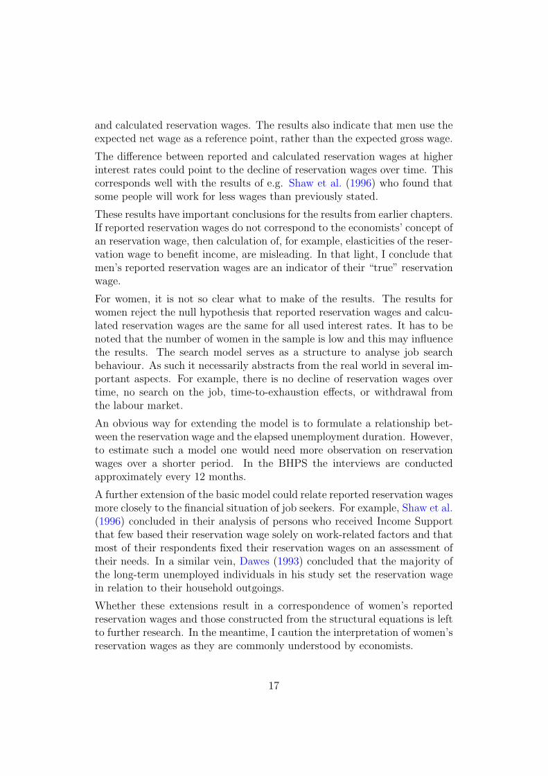
with R2 = 0.003 and N=434. Standard errors in parentheses. The estima-tion clearly suffers from either a small sample size or misspecification of themodel: the R2, of only 0.3%, is low. The corresponding scatterplot is givenin Figure 4.

4.1 Specification checks

Interest rates Of course, the obtained results depend on the assumeddiscount rate and the specifications of the equations. To illustrate the sen-sitivity to the discount rate, I tabulate in Table 6 the estimated parameterswhen other discount rates are chosen. Lower discount rates imply that futureincome is valued more highly at present. Therefore, unemployed job seekerswill not want to search longer for a job offer as the value of search is reduced,i.e. their reservation wage is also lower. This effect can be seen in Table 6where lower discount rates correspond to smaller intercepts. A discount rateof 2 per cent results in a predicted reservation wage that corresponds closelyto reported reservation wages:

ξri = 0.090 + 0.878 ξc

i

(0.096) (0.074).

For men, interest rates in the range of 1 to 3 per cent per annum relate to es-timated parameters which correspond to the hypothesis the model. However,this is not true for the sample of women where the estimations suffer from apoor fit. Varying the interest rate does not change the obtained results to asimilar degree than for men.

Mean completed unemployment duration The calculated reserva-tion wage also depends on the mean completed unemployment duration. Agreater mean completed unemployment duration results in a smaller changeof the reservation wage distribution in reaction to a change of the mean of thewage offer distribution, m. I have re-estimated the system of equations for

14

various values of the mean completed unemployment duration. For example,doubling of the mean completed unemployment duration yields estimatedparameters for men of

ξri = 0.192 + 1.001 ξc

i

(0.094) (0.091),

at an interest rate of 10 per cent per annum. The results for other interestrates are tabulated in Table 7. The obtained model fit is lower than if themean completed unemployment duration of the sample is used. Note thatthe results for women are hardly affected by a changed mean completedunemployment duration.

I have tabulated the results for shorter mean completed unemployment du-rations in Table 8, using a halved mean completed unemployment durationas an example. For men, the estimated relationship between reported andcalculated reservation wages is

ξri = 0.192 + 1.001 ξc

i

(0.094) (0.091).

In general, the hypothesised relationship holds also for interest rates up toabout 10 per cent per annum. Again, the results for women do not changegreatly from the ones obtained above.

Gross wage The estimation above use weekly usual net wage to modelthe wage offer distribution. I have re-estimated the structural equationsusing the weekly usual gross wage. The underlying structural equationschange little, the mean gross wage for men is 223£/week and it is 133£/weekfor women. The log-likelihood for the maximum likelihood estimation of theselection-corrected wage regression for men is with -910 smaller than the -868 obtained when the net wage is used. Similarly, the log-likelihood forwomen is also smaller, -402 vs -378. The association of the predicted wageand the probability of being unemployed is larger when net wages are used,the estimated coefficients for men on predicted gross wage is -3.8 (S.E. 0.7)and it is -3.1 (S.E. 1.4) for women.

The relationship between the calculated and the reported reservation wages,using an interest rate of 10 per cent per annum, is estimated for men as

ξri = 0.629 + 0.675 ξc

i

(0.086) (0.099).

15

Estimated intercept and slope parameters for other interest rates are tabu-lated in Table 9. In general, the estimated intercepts are greater and theestimated slopes are smaller than when net wages are used. Since the un-derlying equations have already a poorer fit with gross wages than with netwages it is not surprising that the R2 are also smaller for these regressions.

The estimated relationship between the ξri and the ξc

i for women can besummarised as follows (for an annual interest rate of 10%)

ξri = 0.857 + 0.230 ξc

i

(0.101) (0.091),

with R2 = 0.024 and N=434. Standard errors in parentheses.

Identifying restrictions The identification of the estimations presentedin Tables 2 and 3 is ensured via the exclusion restrictions. These are thevariables which are assumed to influence the reservation wage but not thejob offer rate. I have estimated the equations with various combinationsof labour market attachment variables (jobs or employer of the previousyear), children in the household, and labour market status of the spouse. Ingeneral, the estimated coefficients are stable with respect to the choice ofexclusion restrictions. The predicted wages differ, taking into account thatthe equations have different explanatory powers; these, however, do not varygreatly. The substantive results do not change: calculated reservation wagesfor men correspond to reported reservation wages at small interest ratesand there is no correspondence between women’s reported and calculatedreservation wages.

5 Summary and conclusion

In this chapter I have related reported reservation wages to reservation wagesobtained from a search model. The calculated reservation wages used infor-mation on accepted wages in jobs following unemployment, completed unem-ployment durations and exogenous discount rates.

For men, at moderate interest rates, I find positive evidence for this simplesearch model. Generally, at interest rates below 5 per cent per annum thehypothesised relationship is supported by the data. This result correspondsto the findings by Schmidt and Winkelmann (1993) who report that an in-terest rate of 6 per cent per annum results in a close match of the reported

16

and calculated reservation wages. The results also indicate that men use theexpected net wage as a reference point, rather than the expected gross wage.

The difference between reported and calculated reservation wages at higherinterest rates could point to the decline of reservation wages over time. Thiscorresponds well with the results of e.g. Shaw et al. (1996) who found thatsome people will work for less wages than previously stated.

These results have important conclusions for the results from earlier chapters.If reported reservation wages do not correspond to the economists’ concept ofan reservation wage, then calculation of, for example, elasticities of the reser-vation wage to benefit income, are misleading. In that light, I conclude thatmen’s reported reservation wages are an indicator of their “true” reservationwage.

For women, it is not so clear what to make of the results. The results forwomen reject the null hypothesis that reported reservation wages and calcu-lated reservation wages are the same for all used interest rates. It has to benoted that the number of women in the sample is low and this may influencethe results. The search model serves as a structure to analyse job searchbehaviour. As such it necessarily abstracts from the real world in several im-portant aspects. For example, there is no decline of reservation wages overtime, no search on the job, time-to-exhaustion effects, or withdrawal fromthe labour market.

An obvious way for extending the model is to formulate a relationship bet-ween the reservation wage and the elapsed unemployment duration. However,to estimate such a model one would need more observation on reservationwages over a shorter period. In the BHPS the interviews are conductedapproximately every 12 months.

A further extension of the basic model could relate reported reservation wagesmore closely to the financial situation of job seekers. For example, Shaw et al.(1996) concluded in their analysis of persons who received Income Supportthat few based their reservation wage solely on work-related factors and thatmost of their respondents fixed their reservation wages on an assessment oftheir needs. In a similar vein, Dawes (1993) concluded that the majority ofthe long-term unemployed individuals in his study set the reservation wagein relation to their household outgoings.

Whether these extensions result in a correspondence of women’s reportedreservation wages and those constructed from the structural equations is leftto further research. In the meantime, I caution the interpretation of women’sreservation wages as they are commonly understood by economists.

17

The introduction of the National Minimum Wage from April 1999 also setsa further research agenda. Before that date, work contracts were basicallyfreely negotiable. It would be worthwhile to investigate whether the Natio-nal Minimum Wage changed people’s search behaviour and reduced the gapbetween reported reservation wages and, ultimately, accepted wages.

18

References

Berthoud, R. (1998). The incomes of ethnic minorities, Institute for Socialand Economic Research, Colchester, UK.

Dawes, L. (1993). Long-term Unemployment and Labour Market Flexibility,Centre for Labour Market Studies, University of Leicester, UK.

Dolton, P. and van der Klaauw, W. (1995). Leaving teacher training in theUK: a duration analysis, Economic Journal 105: 431–444.

Gregg, P. and Wadsworth, J. (1996). How effective are state employmentagencies? jobcentre use and job matching in Britain, Oxford Bulletin ofEconomics and Statistics 58(3): 443–467.

Hannan, C. (1999). Beyond networks: ‘social cohesion’ and unemploymentexit rates, Working Paper 99/28. Institute for Labour Research, Universityof Essex, UK.

Heath, A. and Swann, T. (1999). Reservation wages and the duration ofunemployment, Research discussion paper 1999–02. Economic ResearchDepartment, Reserve Bank of Australia.

Heckman, J. J. (1979). Sample selection bias as a specification error, Econo-metrica 47(1): 153–161.

Institute for Social and Economic Research (1999). British Household PanelSurvey [computer file, study number 4069], UK Data Archive [distributor],Colchester, UK.

Johnson, N. L. and Kotz, S. (1972). Distributions in Statistics: ContinuousMultivariate Distributions, John Wiley & Sons.

Jones, S. R. G. (1988). The relationship between unemployment spells andreservation wages as a test of search theory, Quarterly Journal of Econo-mics 103(4): 741–65.

Kasper, H. (1967). The asking price of labour and the duration of unemploy-ment, The Review of Economics and Statistics 49: 165–72.

Lancaster, T. (1985). Simultaneous equations models in applied searchtheory, Journal of Econometrics 28: 113–126.

Lancaster, T. and Chesher, A. (1983). An econometric analysis of reservationwages, Econometrica 51: 1661–76.

19

Marsh, A. and McKay, S. (1993). Families, Work and Benefits, Policy StudiesInstitute, London.

Office of National Statistics (1998). Regional Trends 33, The StationeryOffice, London.

Osberg, L. (1993). Fishing in different pools: job-search strategies and job-finding success in cananda in the early 1980s, Journal of Labor Economics11(2): 348–386.

Schmidt, C. M. and Winkelmann, R. (1993). Reservation wages, wage offerdistribution and accepted wages, in H. Bunzel, P. Jensen and N. Wes-tergard-Nielsen (eds), Panel Data and Labour Market Dynamics, NorthHolland, Amsterdam.

Shaw, A., Walker, R., Ashworth, K., Jenkins, S. and Middleton, S. (1996).Moving off Income Support: Barriers and Bridges, Department of SocialSecurity Research Report No. 53, London, UK.

Taylor, M. F., Brice, J., Buck, N. and Prentice-Lane, E. (eds) (1998). BritishHousehold Panel Survey User Manual, University of Essex, Colchester,UK.

6 Figures and tables

t t+s t+1time

Start of jobInterview Interview

Observe reportedreservation wagefor all unemployedpersons

Observe acceptedwage for thosewho accepted ajob

Figure 1: Timing of events.

20

Reservation wage equationξc = z γ + ρ=σ ξ=λ ξ

Estimates for γ

Calculation of ρ

Calculation of λξ

Calculation of m

Estimates for β

Exogenous discount rate

Selection-correctedwage regression

Mean completedunemployment duration

ξr = a + b ξc

Figure 2: Estimation strategy.

21

Regression of reported res wage on calculated res wage, 10pc, men.Prediction and C.I.

Rep

orte

d re

serv

atio

n w

age

Calculated reservation wage

.4 .6 .8 1

-2

-1

0

1

2

Figure 3: Reported and calculated reservation wages, 10% p.a., men.

22

Regression of reported res wage on predicted res wage, 10pc, women.Prediction and C.I.

Rep

orte

d re

serv

atio

n w

age

Calculated reservation wage

0 .5 1 1.5

-2

-1

0

1

2

Figure 4: Reported and calculated reservation wages, 10% p.a., women.

23

Table 1: Summary statistics.

Men WomenVariable Mean (S.D.) Mean (S.D.)Wagea (£/week) 177.8 (89.8) 109.0 (58.3)Reservation wageb (£/week) 153.2 (84.0) 154.0 (77.7)Predicted wagec (£/week) 181.4 (44.8) 143.4 (42.6)Personal characteristics

Age (years) 35.1 (13.2) 34.7 (12.7)Education (%)Degree 9.5 8.1A-levels 30.6 29.6O-levels 20.7 22.3Formal qualification below 0-levels 10.9 14.4No formal qualification 28.9 26.6

Ethnic background (%)European 90.6 90.8Black 2.9 2.5Indian 2.2 2.5Pakistani, Bangladeshi 2.1 0.2Other 0.6 4.0

Household characteristics (%)Married 44.5 34.4Cohabiting 12.8 11.8Other 42.7 53.8Spouse has a job 26.8 33.0No child 67.7 72.61 child 11.0 16.72 children 13.1 8.13 or more children 8.1 2.6Youngest child between 0 and 5 years 19.8 14.9Household size (persons) 3.2 (1.4) 2.8 (1.3)

Labour market characteristicsWeeks in job between t-1 and t 21.0 (19.8) 25.0 (21.2)Number of employers, t-1 and t 0.8 (0.7) 0.8 (0.7)Regional unemployment rate 9.1 (2.3) 8.7 (2.3)Region (%)London 15.1 18.7Southeast 16.8 19.6Southwest 7.5 10.7Eastmidlands 22.3 21.5North 26.7 17.2Wales 4.0 4.9Scotland 7.5 7.4

N 739 333

Note: Sample is weighted with cross-sectional weights. Excludes those who fail the consis-tency conditions as derived from the stationary job search model, see text for details.a Sample size (unweighted): 342 men, 211 women. b Sample size: 261 men, 87 women. c

Predicted from estimating equation (11), the results for men are tabulated in Table 2 andfor women in Table 3.

24

Table 2: Results of a selection-corrected wage regression for Britishmen.

Selection regression Wage regressionCoefficient (S.E.) Coefficient (S.E.)

Personal characteristicsAge -0.069 (0.025) 0.066 (0.011)Age2/100 0.055 (0.032) -0.076 (0.014)EducationDegree 0.698 (0.172) 0.420 (0.096)A-levels 0.544 (0.111) 0.201 (0.062)O-levels 0.593 (0.127) 0.093 (0.067)Formal qualification below O-levels 0.226 (0.137) 0.211 (0.089)

Ethnic backgroundBlack 0.176 (0.314) 0.000 (0.092)Indian 0.805 (0.398) -0.131 (0.095)Pakistani, Bangladeshi -0.319 (0.348) 0.162 (0.378)Other 0.838 (0.553) 0.118 (0.197)

Household characteristicsMarried 0.089 (0.119) -0.020 (0.058)Spouse has a job 0.230 (0.107) —No child 0.099 (0.159) 0.040 (0.058)2 children 0.130 (0.164) -0.016 (0.095)3 or more children 0.072 (0.180) 0.021 (0.093)Youngest child between 0 and 5 years -0.316 (0.134) —Household size -0.054 (0.041) —

Labour market characteristicsWeeks in job between t− 1 and t 0.011 (0.003) 0.003 (0.001)Number of employers, t− 1 and t 0.139 (0.079) —Regional unemployment rate -0.119 (0.027) 0.009 (0.013)RegionSoutheast -0.218 (0.218) 0.063 (0.097)Southwest -0.163 (0.233) -0.164 (0.105)Eastmidlands 0.050 (0.176) -0.147 (0.083)North -0.007 (0.159) -0.182 (0.074)Wales -0.026 (0.247) -0.221 (0.105)Scotland -0.001 (0.203) -0.136 (0.082)

Constant 1.788 (0.632) 0.007 (0.257)Estimated parameters

ρ 0.005 (0.226)σw 0.390 (0.021)λw 0.002 (0.088)

N 1213Log-likelihood -868.1

Note: Dependent variables are whether the person is employed (selection equation) andthe wage (in log £/week). Standard errors in parentheses. All variables are measured attime t, except wage which is measured at time t + 1. Omitted categories are: No formalqualification, European, other marital statuses, one dependent child, London.

25

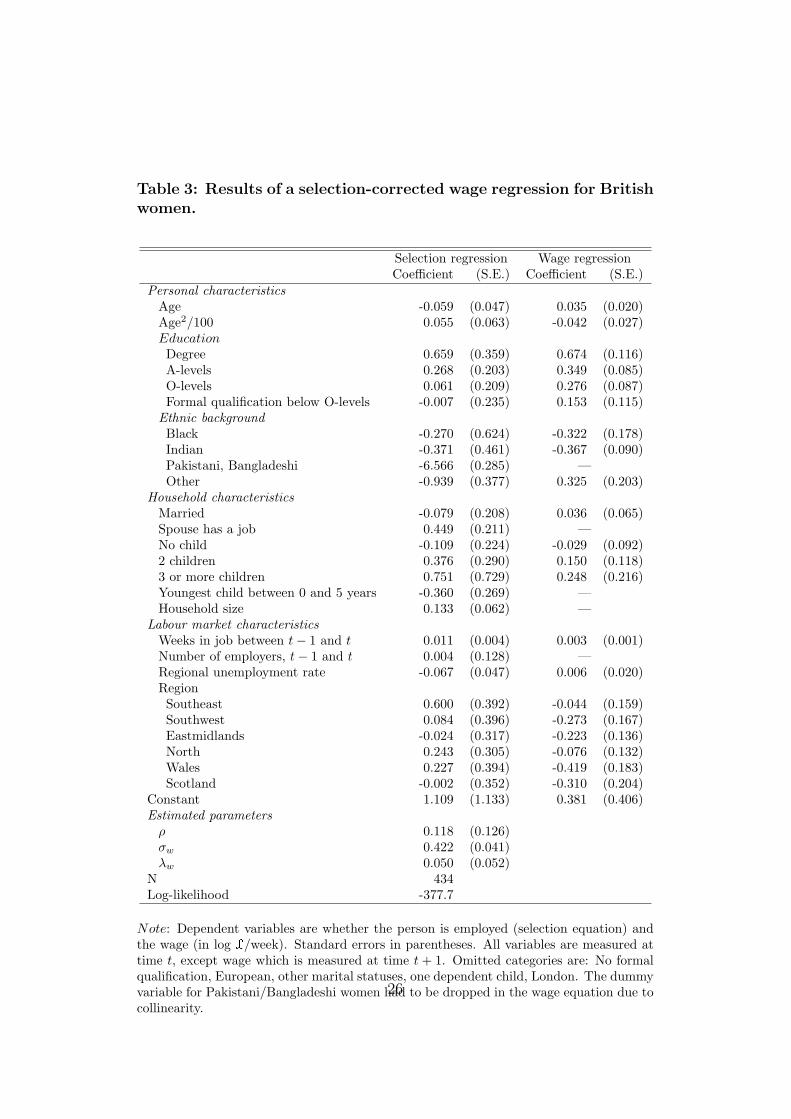
Table 3: Results of a selection-corrected wage regression for Britishwomen.

Selection regression Wage regressionCoefficient (S.E.) Coefficient (S.E.)

Personal characteristicsAge -0.059 (0.047) 0.035 (0.020)Age2/100 0.055 (0.063) -0.042 (0.027)EducationDegree 0.659 (0.359) 0.674 (0.116)A-levels 0.268 (0.203) 0.349 (0.085)O-levels 0.061 (0.209) 0.276 (0.087)Formal qualification below O-levels -0.007 (0.235) 0.153 (0.115)

Ethnic backgroundBlack -0.270 (0.624) -0.322 (0.178)Indian -0.371 (0.461) -0.367 (0.090)Pakistani, Bangladeshi -6.566 (0.285) —Other -0.939 (0.377) 0.325 (0.203)

Household characteristicsMarried -0.079 (0.208) 0.036 (0.065)Spouse has a job 0.449 (0.211) —No child -0.109 (0.224) -0.029 (0.092)2 children 0.376 (0.290) 0.150 (0.118)3 or more children 0.751 (0.729) 0.248 (0.216)Youngest child between 0 and 5 years -0.360 (0.269) —Household size 0.133 (0.062) —

Labour market characteristicsWeeks in job between t− 1 and t 0.011 (0.004) 0.003 (0.001)Number of employers, t− 1 and t 0.004 (0.128) —Regional unemployment rate -0.067 (0.047) 0.006 (0.020)RegionSoutheast 0.600 (0.392) -0.044 (0.159)Southwest 0.084 (0.396) -0.273 (0.167)Eastmidlands -0.024 (0.317) -0.223 (0.136)North 0.243 (0.305) -0.076 (0.132)Wales 0.227 (0.394) -0.419 (0.183)Scotland -0.002 (0.352) -0.310 (0.204)

Constant 1.109 (1.133) 0.381 (0.406)Estimated parameters

ρ 0.118 (0.126)σw 0.422 (0.041)λw 0.050 (0.052)

N 434Log-likelihood -377.7

Note: Dependent variables are whether the person is employed (selection equation) andthe wage (in log £/week). Standard errors in parentheses. All variables are measured attime t, except wage which is measured at time t + 1. Omitted categories are: No formalqualification, European, other marital statuses, one dependent child, London. The dummyvariable for Pakistani/Bangladeshi women had to be dropped in the wage equation due tocollinearity.

26

Table 4: Results of a probit estimation of being unemployed, bysex.

Men WomenCoefficient (S.E.) Coefficient (S.E.)

Predicted log wage (£/week) -5.540 (1.106) -3.836 (1.727)Personal characteristics

Age 0.355 (0.079) 0.141 (0.081)Age2/100 -0.379 (0.092) -0.151 (0.102)EducationDegree 1.808 (0.500) 1.850 (1.174)A-levels 0.561 (0.245) 0.944 (0.661)O-levels 0.087 (0.163) 1.165 (0.517)Formal education below 0-levels 1.132 (0.277) 0.627 (0.362)

Ethnic backgroundBlack 0.095 (0.307) -1.167 (0.868)Indian -0.964 (0.385) -1.890 (0.831)Pakistani, Bangladeshi 1.058 (0.358) 0.326 (0.265)Other -0.514 (0.619) 1.674 (0.570)

Household characteristicsMarried -0.033 (0.119) -0.002 (0.223)Spouse has a job -0.309 (0.107) -0.342 (0.223)No child 0.005 (0.162) -0.076 (0.227)2 children -0.080 (0.154) 0.265 (0.409)3 or more children 0.278 (0.175) 0.858 (0.806)Youngest child between 0 and 5 years 0.252 (0.128) 0.589 (0.265)Household size -0.028 (0.043) -0.205 (0.070)

Labour market characteristicsNumber of employers, t− 1 and t -0.208 (0.084) -0.072 (0.131)Regional unemployment rate 0.123 (0.029) 0.130 (0.051)RegionSoutheast 0.280 (0.242) -0.199 (0.431)Southwest -1.105 (0.299) -1.047 (0.660)Eastmidlands -0.710 (0.231) -0.505 (0.537)North -0.898 (0.248) -0.144 (0.355)Wales -1.019 (0.343) -1.490 (0.838)Scotland -0.717 (0.240) -0.993 (0.674)

Constant 0.085 (0.626) -0.578 (1.344)N 1213 434Log-likelihood -674.7 -228.9Pseudo-R2 0.197 0.185

Note: Standard errors in parentheses. The predicted log wage is obtained from the esti-mation tabulated in Table 2 for men, and Table 3 for women. Omitted categories are: Noformal education, European, other marital statuses, one dependent child, London.

27

Table 5: Results of a reservation wage regression, by sex.

Men WomenCoefficient (S.E.) Coefficient (S.E.)

Personal characteristicsAge 0.037 (0.012) 0.059 (0.020)Age2/100 -0.044 (0.017) -0.058 (0.023)

EducationDegree 0.491 (0.118) -0.093 (0.574)A-levels 0.272 (0.124) 0.135 (0.252)O-levels 0.151 (0.089) 0.357 (0.113)Formal education below 0-levels 0.044 (0.061) 0.241 (0.096)

Ethnic backgroundBlack -0.032 (0.086) 0.373 (0.159)Indian 0.286 (0.152) -0.561 (0.392)Pakistani, Bangladeshi 0.029 (0.079) 0.148 (0.138)Other 0.230 (0.291) -0.091 (0.309)

Household characteristicsMarried 0.122 (0.052) -0.089 (0.137)Spouse has a job 0.019 (0.078) -0.117 (0.197)No child -0.113 (0.080) 0.046 (0.111)2 children 0.090 (0.058) -0.308 (0.196)3 or more children 0.328 (0.077) 0.079 (0.217)Youngest child between 0 and 5 years 0.121 (0.070) 0.585 (0.303)

Household size -0.311 (0.020) -0.452 (0.112)Labour market characteristics

Number of weeks employed, t− 1 and t 0.006 (0.004) -0.008 (0.007)Number of employers, t− 1 and t -0.058 (0.055) -0.018 (0.087)Regional unemployment rate 0.007 (0.017) 0.026 (0.049)Region

Southeast -0.032 (0.093) -0.484 (0.206)Southwest -0.067 (0.105) -0.496 (0.220)Eastmidlands -0.055 (0.076) -0.133 (0.196)North -0.157 (0.071) -0.101 (0.178)Wales -0.193 (0.103) -0.087 (0.153)Scotland -0.132 (0.080) -0.035 (0.177)

λξ -0.274 (0.352) 0.899 (0.879)Constant 1.513 (0.438) 0.073 (1.248)N 516 124R2 0.643 0.693

Note: Dependent variable is the reservation wage in log £/week. Standard errors in pa-rentheses. Omitted categories are: No formal education, European, other marital statuses,one dependent child, London.

28

Table 6: Relationship between predicted and calculated reservationwages at different interest rates.

Interest rate per annum (%) Intercept (S.E.) Slope (S.E.) R2

Men, N=12131 0.062 (0.096) 0.834 (0.069) 0.1712 0.090 (0.96)) 0.878 (0.074) 0.1665 0.192 (0.093) 1.006 (0.091) 0.14610 0.436 (0.088) 1.152 (0.128) 0.10315 0.772 (0.075) 1.042 (0.175) 0.049

Women, N=4341 0.914 (0.091) 0.208 (0.096) 0.0172 0.927 (0.090) 0.203 (0.098) 0.0155 0.965 (0.086) 0.180 (0.105) 0.01010 1.028 (0.079) 0.121 (0.115) 0.00315 1.089 (0.071) 0.033 (0.125) 0.000

Note: Standard errors in parentheses. Regression of predicted reservation wages on cal-culated reservation wages. See text for details.

Table 7: Relationship between predicted and calculated reservationwages at different interest rates, for a doubled mean completedunemployment duration.

Interest rate per annum (%) Intercept (S.E.) Slope (S.E.) R2

Men, N=12131 0.090 (0.096) 0.878 (0.074) 0.1662 0.155 (0.095) 0.965 (0.085) 0.1535 0.436 (0.088) 1.152 (0.128) 0.10310 1.092 (0.048) 0.455 (0.217) 0.00615 1.053 (0.027) -1.293 (0.243) 0.045

Women, N=4341 0.927 (0.090) 0.203 (0.098) 0.0152 0.952 (0.088) 0.189 (0.102) 0.0125 1.028 (0.078) 0.121 (0.115) 0.00310 1.139 (0.063) -0.081 (0.134) 0.00115 1.196 (0.048) -0.358 (0.150) 0.015

Note: Standard errors in parentheses. Regression of predicted reservation wages on cal-culated reservation wages. See text for details.

29

Table 8: Relationship between predicted and calculated reserva-tion wages at different interest rates, for a halved mean completedunemployment duration.

Interest rate per annum (%) Intercept (S.E.) Slope (S.E.) R2

Men, N=12131 0.049 (0.096) 0.812 (0.067) 0.1742 0.062 (0.096) 0.834 (0.069) 0.1715 0.105 (0.095) 0.900 (0.077) 0.16310 0.192 (0.094) 1.006 (0.091) 0.14615 0.302 (0.092) 1.097 (0.108) 0.126

Women, N=4341 0.908 (0.092) 0.210 (0.095) 0.0182 0.914 (0.091) 0.208 (0.096) 0.0175 0.933 (0.089) 0.200 (0.099) 0.01410 0.965 (0.086) 0.180 (0.105) 0.01015 0.997 (0.082) 0.154 (0.110) 0.006

Note: Standard errors in parentheses. Regression of predicted reservation wages on cal-culated reservation wages. See text for details.

Table 9: Relationship between predicted and calculated reservationwages at different interest rates, gross wage.

Interest rate per annum (%) Intercept (S.E.) Slope (S.E.) R2

Men, N=12131 0.093 (0.102) 0.653 (0.058) 0.1452 0.142 (0.100) 0.673 (0.062) 0.1365 0.307 (0.097) 0.712 (0.075) 0.11010 0.629 (0.086) 0.675 (0.099) 0.06215 0.947 (0.067) 0.459 (0.121) 0.020

Women, N=4341 0.842 (0.102) 0.233 (0.089) 0.0262 0.857 (0.101) 0.230 (0.091) 0.0245 0.903 (0.096) 0.213 (0.098) 0.01710 0.981 (0.086) 0.164 (0.108) 0.00815 1.054 (0.077) 0.085 (0.117) 0.002

Note: Standard errors in parentheses. Regression of predicted reservation wages on cal-culated reservation wages.

30