1 Regularisierung mir Singulären Energien Martin Burger Institut für Numerische und Angewandte...

1

Regularisierung mir Singulären Energien

Martin Burger

Institut für Numerische und Angewandte MathematikWestfälische Wilhelms Universität Münster

[email protected]

Regularisierung mit singulären Energien

Göttingen, Januar 2007 2

Stan Osher, Jinjun Xu, Guy Gilboa (UCLA)

Lin He (Linz / UCLA)

Klaus Frick, Otmar Scherzer (Innsbruck)

Carola Schönlieb (Vienna)

Don Goldfarb, Wotao Yin (Columbia)

Collaborations



Classical regularization schemes for inverse problems and image smoothing are based on Hilbert spaces and quadratic energy functionals

Example: Tikhonov regularization for linear operator equations

Introduction

¸2kAu ¡ f k2+

12kLuk2 ! min

u

¸2kAu ¡ f k2+

12kLuk2 ! min

u



These energy functionals are strictly convex and differentiable – standard tools from analysis and computation (Newton methods etc.) can be used Disadvantage: possible oversmoothing, seen from first-order optimality condition Tikhonov yields

Hence u is in the range of (L*L)-1A*

Introduction

¸2kAu ¡ f k2+

12kLuk2 ! min

u

L¤Lu = ¡ ¸A¤(Auf )



Classical inverse problem: integral equation of the first kind, regularization in L2 (L = Id), A = Fredholm integral operator with kernel k

Smoothness of regularized solution is determined by smoothness of kernel For typical convolution kernels like Gaussians, u is analytic !

Introduction

¸2kAu ¡ f k2+

12kLuk2 ! min

u

u= ¸Z Z

k(y;x)(¡ k(y;z)u(z) + f (z)) dy dz



Classical image smoothing: data in L2 (A = Id), L = gradient (H1-Seminorm)

On a reasonable domain, standard elliptic regularity implies

Reconstruction contains no edges, blurs the image (with Green kernel)

Image Smoothing

¸2kAu ¡ f k2+

12kLuk2 ! min

u

¡ ¢ u+¸u = ¸f

u 2 H 2( ) ,! C( )



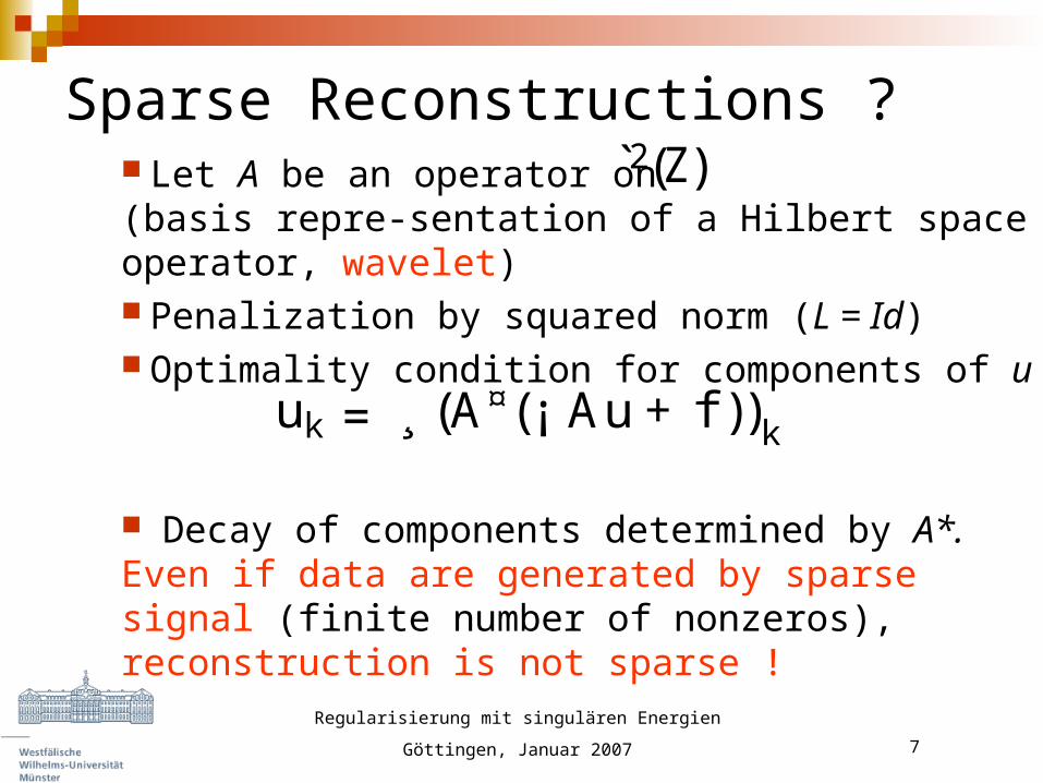
Let A be an operator on (basis repre-sentation of a Hilbert space operator, wavelet) Penalization by squared norm (L = Id) Optimality condition for components of u

Decay of components determined by A*. Even if data are generated by sparse signal (finite number of nonzeros), reconstruction is not sparse !

Sparse Reconstructions ?

¸2kAu ¡ f k2+

12kLuk2 ! min

u

2̀(Z)

uk = ¸ (A¤(¡ Au+ f ))k



Error estimates for ill-posed problems can be obtained only under stronger conditions (source conditions)

cf. Groetsch, Engl-Hanke-Neubauer, Colton-Kress, Natterer. Engl-Kunisch-Neubauer. Equivalent to u being minimizer of Tikhonov functional with data For many inverse problems unrealistic due to extreme smoothness assumptions

Error estimates

¸2kAu ¡ f k2+

12kLuk2 ! min

u

9w : u = A¤w



Condition can be weakened to

cf. Neubauer et al (algebraic), Hohage (logarithmic), Mathe-Pereverzyev (general).

Advantage: more realistic conditions

Disadvantage: Estimates get worse with f

Error estimates

¸2kAu ¡ f k2+

12kLuk2 ! min

u

9v : u = f (A¤A)v



Let A be the identity on Nonlinear Penalization by Optimality condition for components of u

If rk is smooth and strictly convex, then Taylor expansion yields

Singular Energies

¸2kAu ¡ f k2+

12kLuk2 ! min

u

2̀(Z)Prk(uk)

r00k (f k)uk +¸uk ¼r00k (f k)f k +¸f k

r0k(uk) +¸uk = ¸f k



Example becomes more interesting for singular (nonsmooth) energy

Take

Then optimality condition becomes

Singular Energies

¸2kAu ¡ f k2+

12kLuk2 ! min

u

rk(t) = jtj

sign (uk) +¸uk = ¸f k



Result is well-known soft-thresholding of wavelets Donoho et al, Chambolle et al

Yields a sparse signal

Singular Energies

¸2kAu ¡ f k2+

12kLuk2 ! min

u

uk =

8<

:

f k ¡ 1¸ f k > 1

¸f k + 1

¸ f k < ¡ 1¸

0 else



Image smoothing: try nonlinear energy

for penalization

Optimality condition is nonlinear PDE

If r is strictly convex usual smoothing behaviour If r is not convex problem not well-posed Try singular case at the borderline

Singular Energies

¸2kAu ¡ f k2+

12kLuk2 ! min

u

Zr(r u)

¡ r ¢((r r)(r u)) +¸u= ¸f



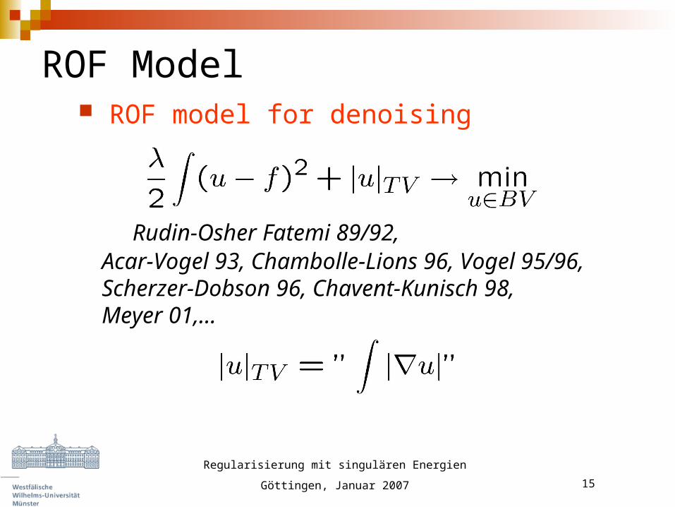
Simplest choice yields total variation method Total variation methods are popular in imaging (and inverse problems), since

- they keep sharp edges- eliminate oscillations (noise)- create new nice mathematics

Total Variation Methodsr(p) = jpj



ROF model for denoising

Rudin-Osher Fatemi 89/92, Acar-Vogel 93, Chambolle-Lions 96, Vogel 95/96, Scherzer-Dobson 96, Chavent-Kunisch 98, Meyer 01,…

ROF Model



Optimality condition for ROF denoising

Dual variable p enters !

Subgradient of convex functional

ROF Model

p+¸u= ¸f ; p2 @jujT V

@J (u) = fp2 X ¤ j 8v 2 X :

J (u) ¡ hp;v ¡ ui · J (v)g



ROF ModelReconstruction (code by Jinjun Xu)

clean noisy ROF



ROF model denoises cartoon images resp. computes the cartoon of an arbitrary image

ROF Model



From Master Thesis of Markus Bachmayr, 2007

Numerical Differentiation with TV



Methods with singular energies offer great potential, but still have some shortcomings

- difficult to analyze and to obtain error estimates- systematic errors (clean images not reconstructed perfectly)- computational challenges- some extensions to complicated imaging tasks are not well understood (e.g. inpainting)

Singular energies



General problem

leads to optimality condition

First of all „dual smoothing“, subgradient p is in the range of A*

Singular energies

¸2kAu ¡ f k2+J (u) ! min

u

p+¸A¤Au= ¸A¤f ; p2 @J (u)



For smooth and strictly convex energies, the subdifferential is a singleton

Dual smoothing directly results in a primal one ! For singular energies, subdifferentials are not usually multivalued. The consequence is a possibility to break the primal smoothing

Singular energies

@J (u) = f J 0(u)g



First question for error estimation: estimate difference of u (minimizer of ROF) and f in terms of

Estimate in the L2 norm is standard, but does not yield information about edges

Estimate in the BV-norm too ambitious: even arbitrarily small difference in edge location can yield BV-norm of order one !

Error Estimation



We need a better error measure, stronger than L2, weaker than BV Possible choice: Bregman distance Bregman 67

Real distance for a strictly convex differentiable functional – not symmetric Symmetric version

Error Estimation



Bregman distances reduce to known measures for standard energies Example 1:

Subgradient = Gradient = u Bregman distance becomes

Error Estimation

J (u) =12kuk2

DJ (u;v) =12ku ¡ vk2



Bregman distances reduce to known measures for standard energies Example 2: -

Subgradient = Gradient = log u Bregman distance becomes Kullback-Leibler divergence (relative Entropy)

Error Estimation

J (u) =

Zulogu

Zu

DJ (u;v) =

Zulog

uv+Z(v¡ u)



Total variation is neither symmetric nor differentiable Define generalized Bregman distance for each subgradient

Symmetric version

Kiwiel 97, Chen-Teboulle 97

Error Estimation



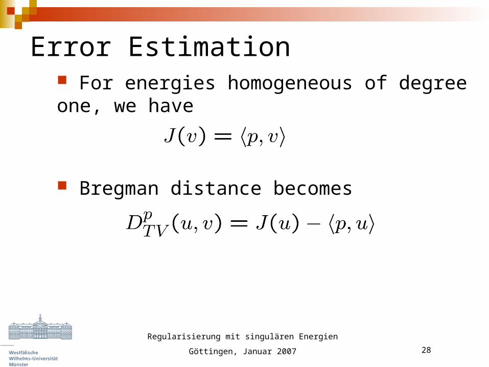
For energies homogeneous of degree one, we have

Bregman distance becomes

Error Estimation



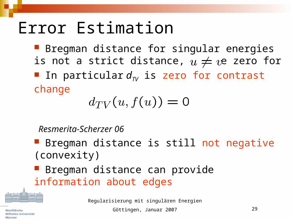
Bregman distance for singular energies is not a strict distance, can be zero for In particular dTV is zero for contrast change

Resmerita-Scherzer 06

Bregman distance is still not negative (convexity) Bregman distance can provide information about edges

Error Estimation



Let v be piecewise constant with white background and color values on regions Then we obtain subgradients of the form

with signed distance function and

Error Estimation



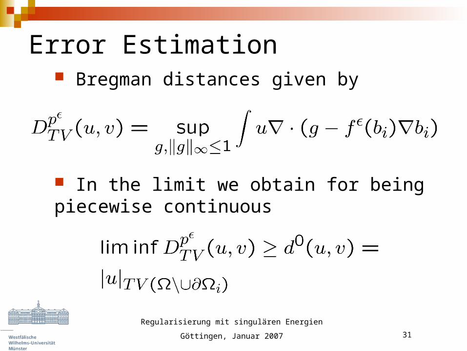
Bregman distances given by

In the limit we obtain for being piecewise continuous

Error Estimation



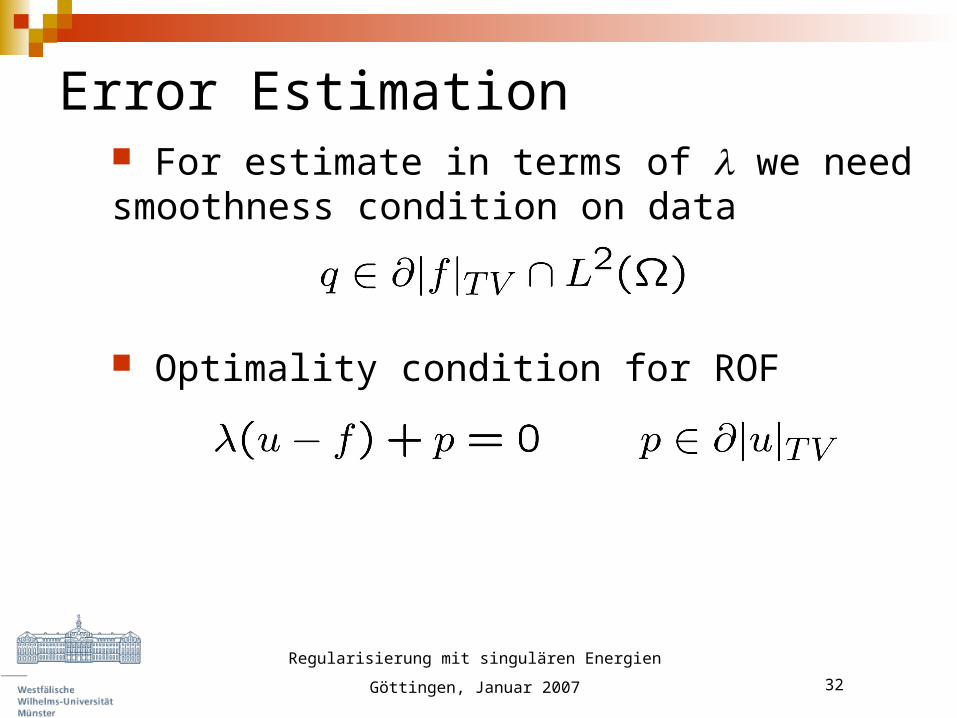
For estimate in terms of we need smoothness condition on data

Optimality condition for ROF

Error Estimation



Subtract q

Estimate for Bregman distance, mb-Osher 04

Error Estimation



In practice we have to deal with noisy data f (perturbation of some exact data g)

Estimate for Bregman distance

Error Estimation



Optimal choice of the penalization parameter

i.e. of the order of the noise variance

Error Estimation



Direct extension to deconvolution / linear inverse problems

under standard source condition

mb-Osher 04 Extension: stronger estimates under stronger conditions, Resmerita 05

Nonlinear inverse problems, Resmerita-Scherzer 06

Error Estimation

¸2kAu ¡ f k2+jujT V ! min

u2B V



Natural choice: primal discretization with piecewise constant functions on grid

Problem 1: Numerical analysis (characterization of discrete subgradients) Problem 2: Discrete problems are the same for any anisotropic version of the total variation

Discretization



In multiple dimensions, nonconvergence of the primal discretization for the isotropic TV (p=2) can be shown

Convergence of anisotropic TV (p=1) on rectangular aligned grids Fitzpatrick-Keeling 1997

Discretization



Alternative: perform primal-dual discretization for optimality system (variational inequality)

with convex set

Primal-Dual Discretization



Discretization

Discretized convex set with appropriate elements (piecewise linear in 1D, Raviart-Thomas in multi-D)

Primal-Dual Discretization



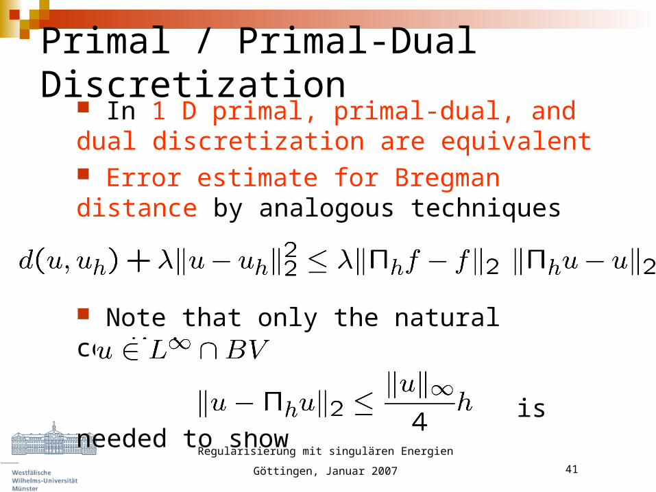
In 1 D primal, primal-dual, and dual discretization are equivalent Error estimate for Bregman distance by analogous techniques

Note that only the natural condition is needed to show

Primal / Primal-Dual Discretization



In multi-D similar estimates, additional work since projection of subgradient is not discrete subgradient.

Primal-dual discretization equivalent to discretized dual minimization (Chambolle 03,

Kunisch-Hintermüller 04). Can be used for existence of discrete solution, stability of p

Mb 07 ?

Primal / Primal-Dual Discretization



For most imaging applications Cartesian grids are used. Primal dual discretization can be reinterpreted as a finite difference scheme in this setup. Value of image intensity corresponds to color in a pixel of width h around the grid point. Raviart-Thomas elements on Cartesian grids particularly easy. First component piecewise linear in x, pw constant in y,z, etc. Leads to simple finite difference scheme with staggered grid

Cartesian Grids



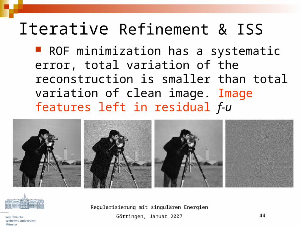
ROF minimization has a systematic error, total variation of the reconstruction is smaller than total variation of clean image. Image features left in residual f-u

g, clean f, noisy u, ROF f-u

Iterative Refinement & ISS



Idea: add the residual („noise“) back to the image to pronounce the features decreased to much. Then do ROF again. Iterative procedure

Osher-mb-Goldfarb-Xu-Yin 04




Improves reconstructions significantly




Simple observation from optimality condition

Consequently, iterative refinement equivalent to Bregman iteration




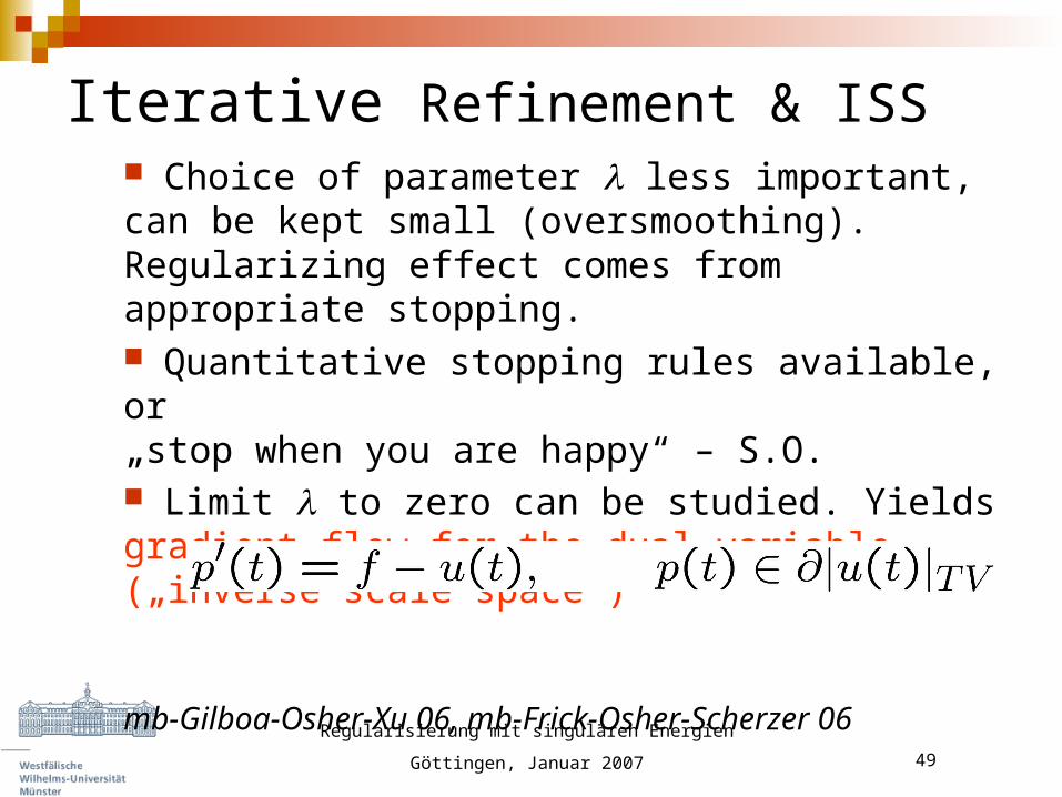
Choice of parameter less important, can be kept small (oversmoothing). Regularizing effect comes from appropriate stopping. Quantitative stopping rules available, or „stop when you are happy“ – S.O. Limit to zero can be studied. Yields gradient flow for the dual variable („inverse scale space“)

mb-Gilboa-Osher-Xu 06, mb-Frick-Osher-Scherzer 06




Non-quadratic fidelity is possible, some caution needed for L1 fidelityHe-mb-Osher 05, mb-Frick-Osher-Scherzer 06

Error estimation in Bregman distance mb-He-Resmerita 07




MRI Data Siemens Magnetom Avanto 1.5 T Scanner He, Chang, Osher, Fang, Speier 06

PenalizationTV + Wavelet

Iterative Refinement



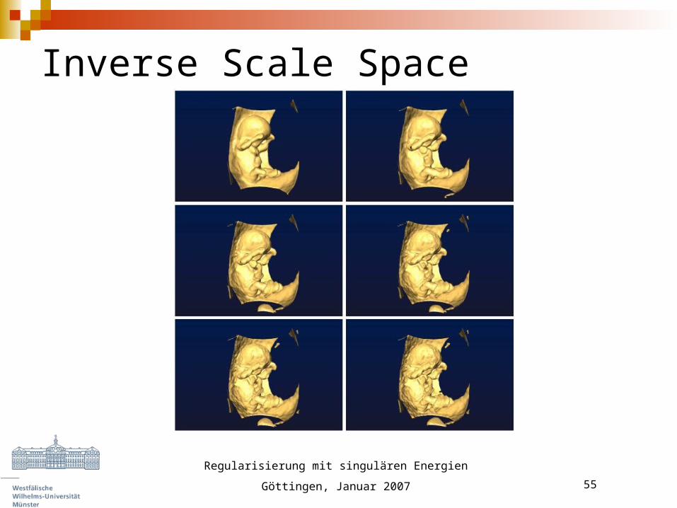
Smoothing of surfaces obtained as level sets

3D Ultrasound, Kretz / GE Med.

Surface Smoothing



Inverse Scale Space



Application to other regularization techniques, e.g. wavelet thresholding is straightforward

Starting from soft shrinkage, iterated refinement yields firm shrinkage, inverse scale space becomes hard shrinkageOsher-Xu 06

Bregman distance natural sparsity measure, source condition just requires sparse signal, number of nonzero components is smoothness measure in error estimates




Difficult to construct total variation techniques for inpainting Original extensions of ROF failed to obtain natural connectivity (see book by Chan, Shen 05)

Inpainting region , image f (noisy) given on Try to minimize

Inpainting



Optimality condition will have the form

with A being a linear operator defining the norm

In particular p = 0 in D !

Inpainting



Different iterated approach (motivated by Cahn-Hilliard inpainting, Bertozzi et al 05) Minimize in each step

First term for damping, second for fidelity (fit to f where given, and to old iterate in the inpainting region), third term for smoothing

Inpainting



Continuous flow for damping parameter to zero

Fourth order flow for H-1 norm

Stationary solution (existence ?) satisfies

Inpainting



Result: Penguins

Inpainting



Download and Contact

Papers and Talks:

www.math.uni-muenster.de/u/burger

e-mail: [email protected]

1 Regularisierung mir Singulären Energien Martin Burger Institut für Numerische und Angewandte...

Documents

Transcript of 1 Regularisierung mir Singulären Energien Martin Burger Institut für Numerische und Angewandte...