1

Psych 5510/6510

Chapter Eight--Multiple Regression: Models with Multiple Continuous Predictors

Part 1: Testing the Overall Model

Spring, 2009

2

Multiple Regression MODEL

Ŷi=β0+ β1Xi1+ β2Xi2+ ...+βp-1Xip-1

This is the general linear model (linear because the separate components, after being weighted by β, are added together). Nonlinear models can be expressed this way too by clever use of predictor variables (we will do that later this semester)

p=number of parameters, as the first parameter is β0

the last will be βp-1

(p-1)=number of predictor variables (X)

3

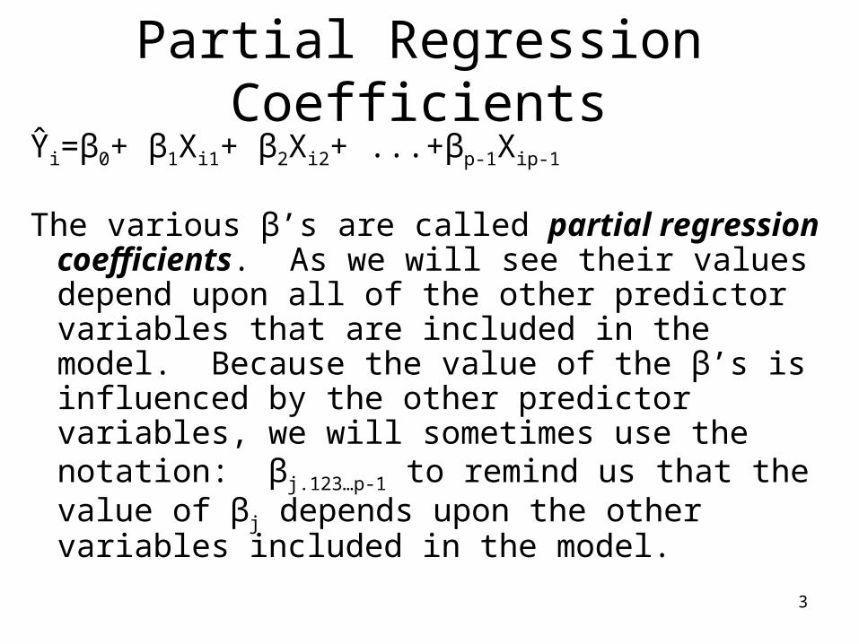
Partial Regression Coefficients

Ŷi=β0+ β1Xi1+ β2Xi2+ ...+βp-1Xip-1

The various β’s are called partial regression coefficients. As we will see their values depend upon all of the other predictor variables that are included in the model. Because the value of the β’s is influenced by the other predictor variables, we will sometimes use the notation: βj.123…p-1 to remind us that the value of βj depends upon the other variables included in the model.

4

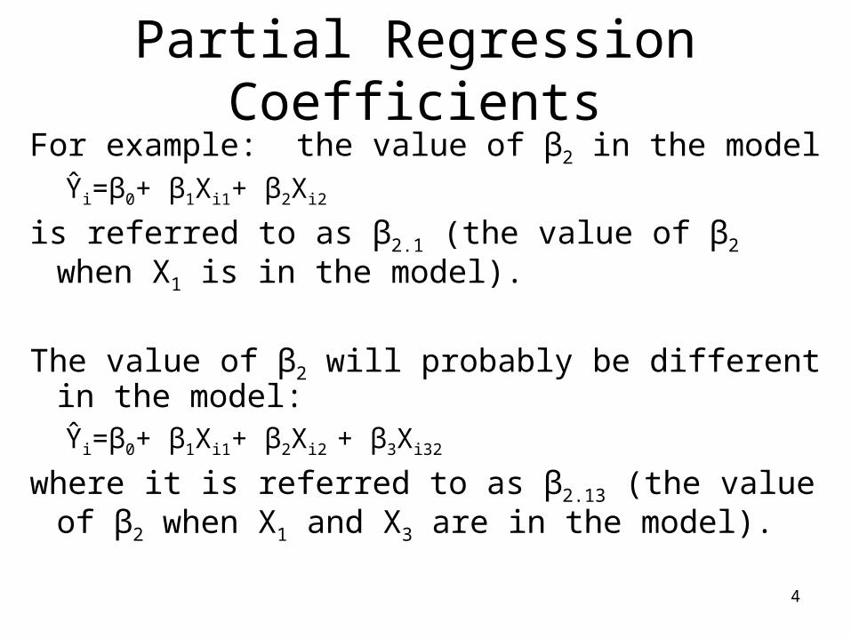
Partial Regression CoefficientsFor example: the value of β2 in the model

Ŷi=β0+ β1Xi1+ β2Xi2

is referred to as β2.1 (the value of β2 when X1 is in the model).

The value of β2 will probably be different in the model:Ŷi=β0+ β1Xi1+ β2Xi2 + β3Xi32

where it is referred to as β2.13 (the value of β2 when X1 and X3 are in the model).

5

RedundancyWhen we use more than one predictor variable

in our model then an important issue arises; specifically, to what degree are the predictor variables redundant (i.e. share information).

6

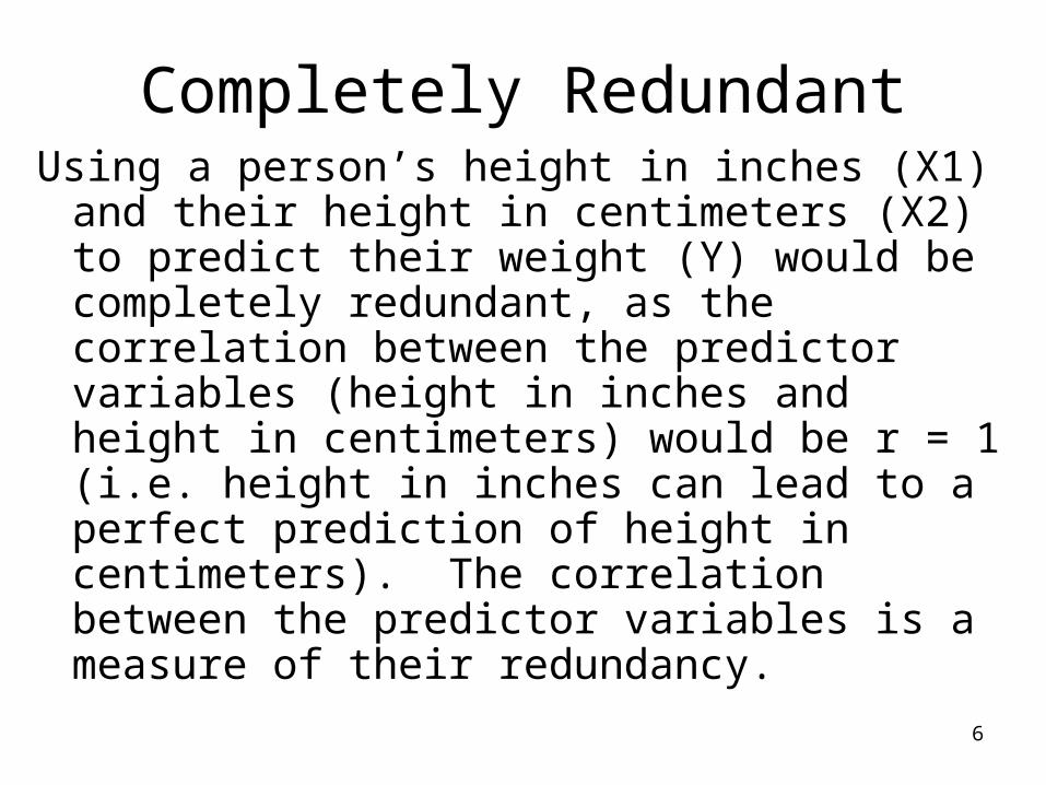
Completely RedundantUsing a person’s height in inches (X1) and

their height in centimeters (X2) to predict their weight (Y) would be completely redundant, as the correlation between the predictor variables (height in inches and height in centimeters) would be r = 1 (i.e. height in inches can lead to a perfect prediction of height in centimeters). The correlation between the predictor variables is a measure of their redundancy.

7

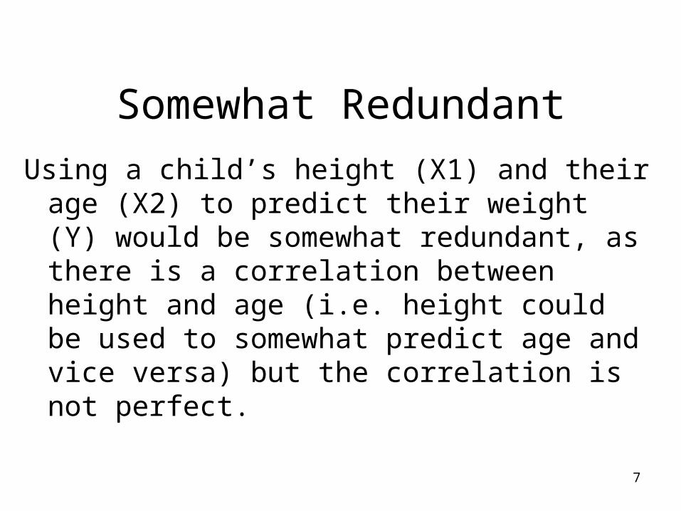
Somewhat Redundant

Using a child’s height (X1) and their age (X2) to predict their weight (Y) would be somewhat redundant, as there is a correlation between height and age (i.e. height could be used to somewhat predict age and vice versa) but the correlation is not perfect.

8

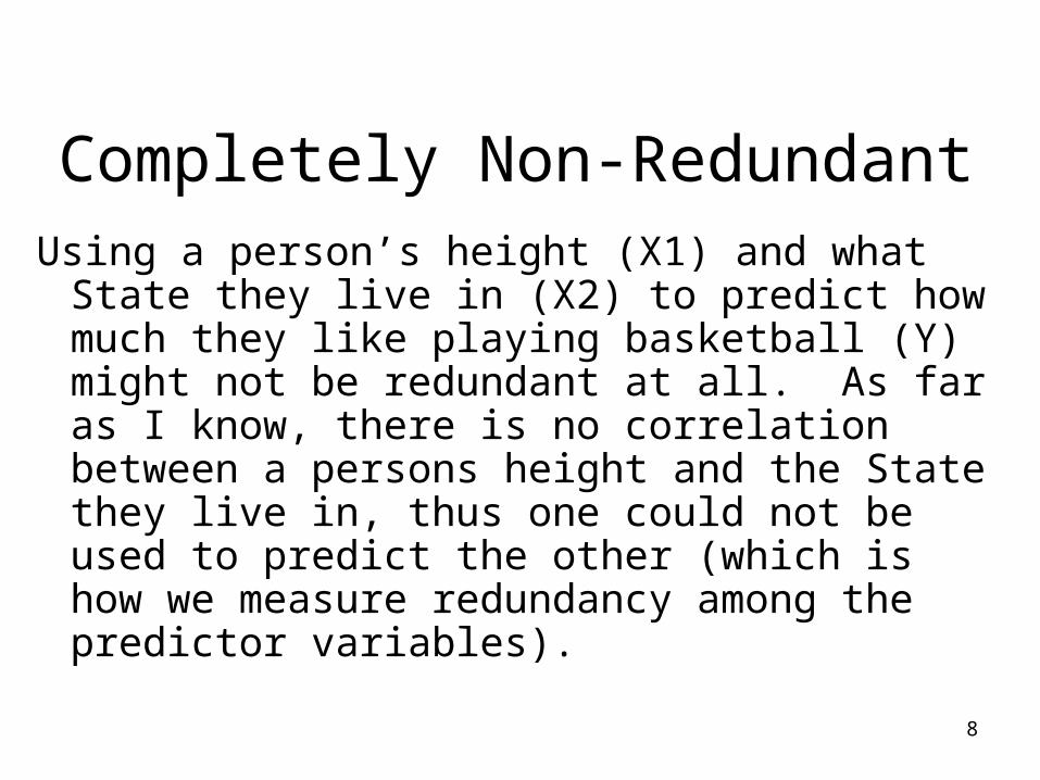
Completely Non-Redundant

Using a person’s height (X1) and what State they live in (X2) to predict how much they like playing basketball (Y) might not be redundant at all. As far as I know, there is no correlation between a persons height and the State they live in, thus one could not be used to predict the other (which is how we measure redundancy among the predictor variables).

9

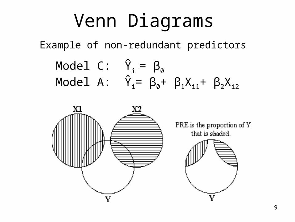
Venn DiagramsExample of non-redundant predictors

Model C: Ŷi = β0

Model A: Ŷi= β0+ β1Xi1+ β2Xi2

10

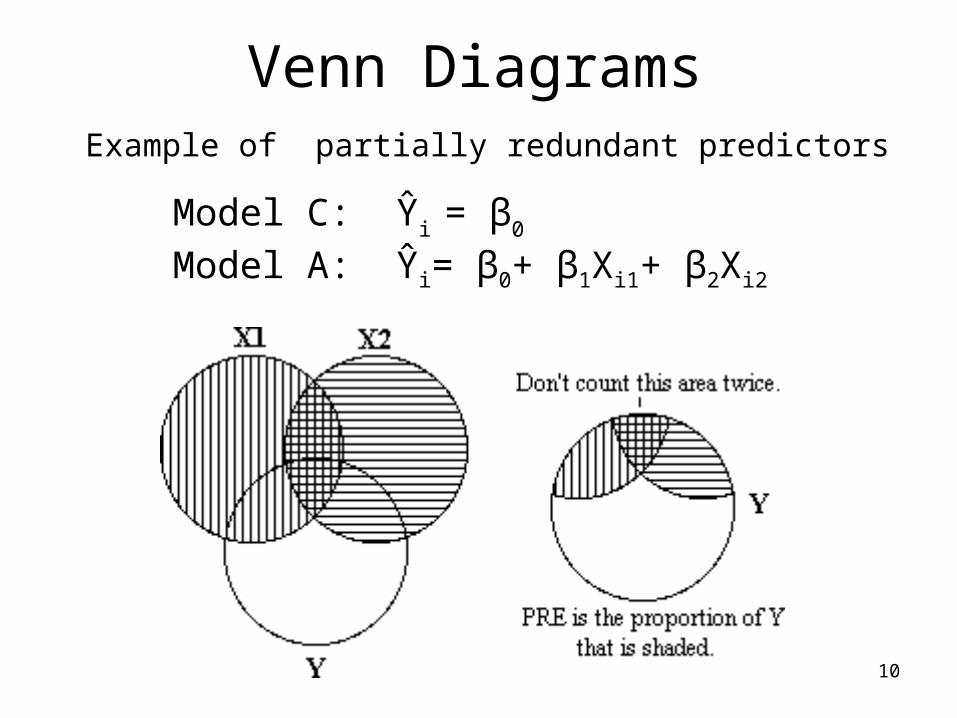
Venn DiagramsExample of partially redundant predictors

Model C: Ŷi = β0

Model A: Ŷi= β0+ β1Xi1+ β2Xi2

11

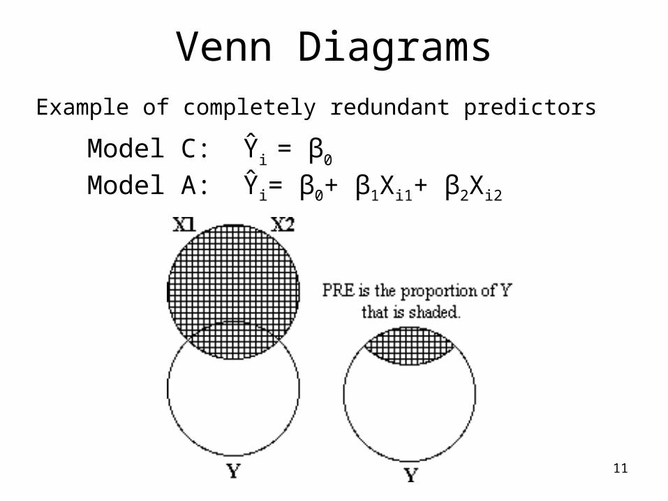
Venn DiagramsExample of completely redundant predictors

Model C: Ŷi = β0

Model A: Ŷi= β0+ β1Xi1+ β2Xi2

12

Estimating parameters

We are going to use the general linear model for predicting values of Y.

Ŷi=β0+ β1Xi1+ β2Xi2+ ...+βp-1Xip-1, or in terms of our estimates of those β’s:

1-ip1-pi33i22i110i Xb...XbXbXbbY

13

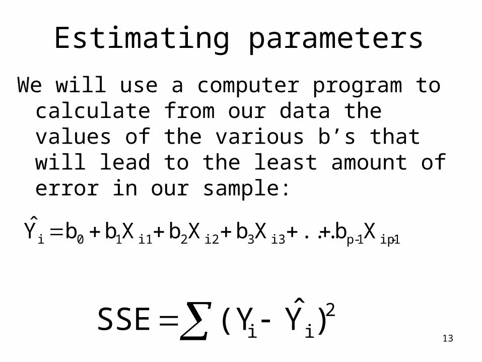
Estimating parameters

We will use a computer program to calculate from our data the values of the various b’s that will lead to the least amount of error in our sample:

2ii )Y (Y SSE

1-ip1-pi33i22i110i Xb...XbXbXbbY

14

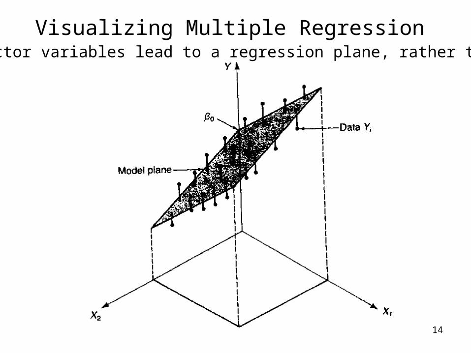
Visualizing Multiple Regression2 predictor variables lead to a regression plane, rather than line.

15

Statistical Inference in Multiple Regression

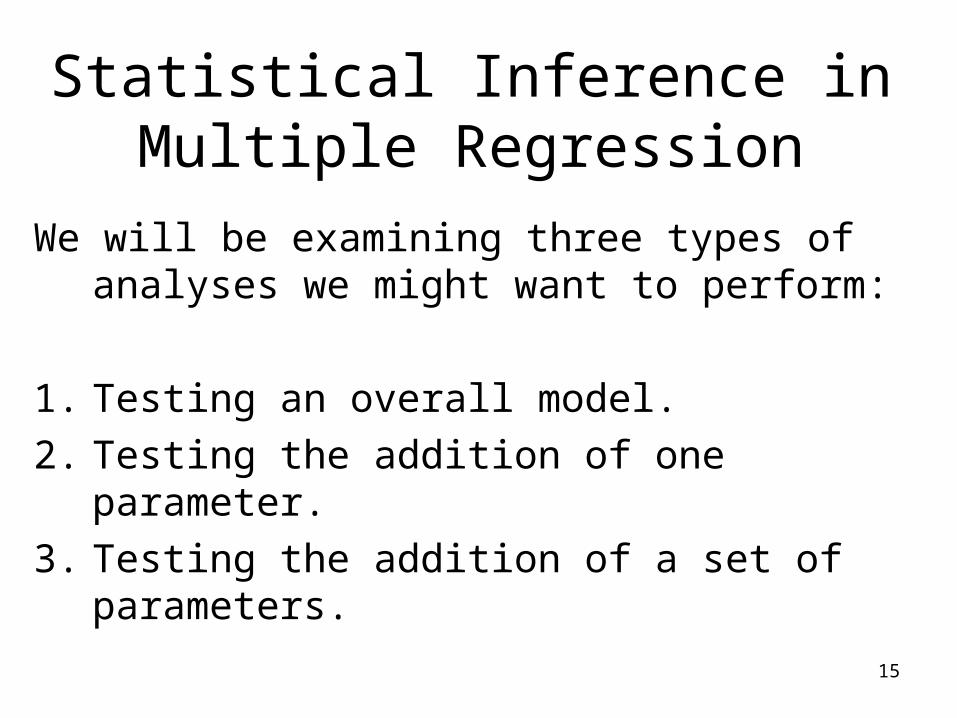
We will be examining three types of analyses we might want to perform:

1. Testing an overall model.

2. Testing the addition of one parameter.

3. Testing the addition of a set of parameters.

16

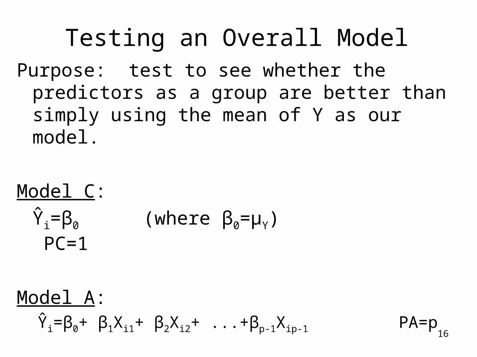
Testing an Overall ModelPurpose: test to see whether the predictors

as a group are better than simply using the mean of Y as our model.

Model C:

Ŷi=β0 (where β0=μY) PC=1

Model A: Ŷi=β0+ β1Xi1+ β2Xi2+ ...+βp-1Xip-1 PA=p

17

As Always

SSE(C)

SSR

SSE(C)

SSE(A)-SSE(C)

SE(C)

SSE(A)1 PRE

SSE(A) - SSE(C) SSR

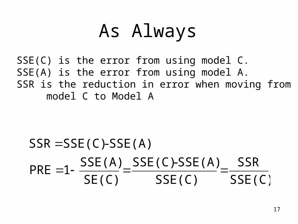
SSE(C) is the error from using model C.SSE(A) is the error from using model A.SSR is the reduction in error when moving from model C to Model A

18

Coefficient of Multiple Determination

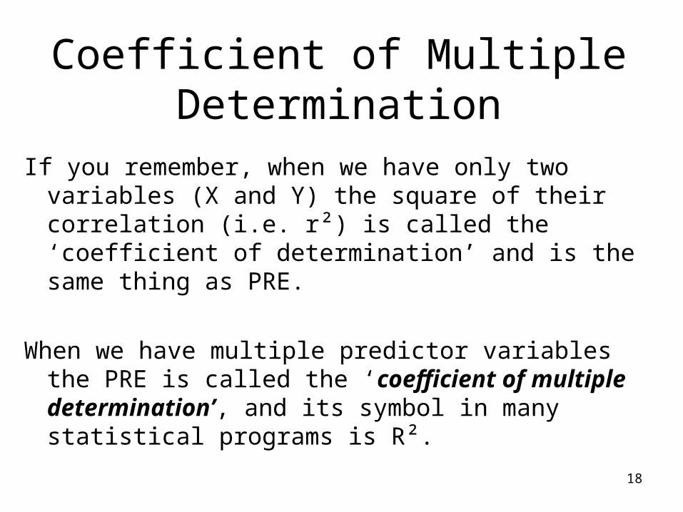
If you remember, when we have only two variables (X and Y) the square of their correlation (i.e. r²) is called the ‘coefficient of determination’ and is the same thing as PRE.

When we have multiple predictor variables the PRE is called the ‘coefficient of multiple determination’, and its symbol in many statistical programs is R².

19

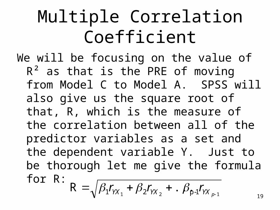
Multiple Correlation Coefficient

We will be focusing on the value of R² as that is the PRE of moving from Model C to Model A. SPSS will also give us the square root of that, R, which is the measure of the correlation between all of the predictor variables as a set and the dependent variable Y. Just to be thorough let me give the formula for R:

121 1-p21 ...R

pYXYXYX rrr

20

Testing Significance

Model C: Ŷi=β0

Model A: Ŷi=β0+ β1Xi1+ β2Xi2+ ...+βp-1Xip-1

We have our three ways of testing the statistical significance of PRE;

1. Look up the PRE critical value.2. The PRE to F* approach.3. The MS to F* approach.

If we reject H0 we say that the whole set of extra parameters of Model A is worthwhile to add to our model (compared to a model consisting only of the mean of Y).

21

MS to F* Method

SPSS will perform the exact test we want here as a linear regression analysis. When SPSS does linear regression, it always assumes the Model C is simply the mean of Y, which is the correct Model C for testing the overall model.

22

Example of an Overall Model Test

Y=College GPA (1st year accumulative)

Predictor variables:X1: High school percentile rank (HSRANK)X2: SAT verbal score (SATV)X3: SAT math score (SATM)

Model C: Ŷi = β0

Model A: Ŷi = β0 + β1Xi1 +β2Xi2 + β3Xi3

23

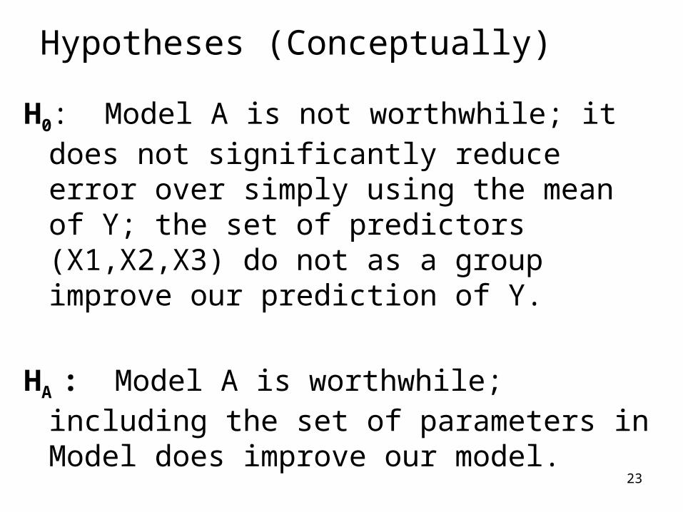
Hypotheses (Conceptually)

H0: Model A is not worthwhile; it does not significantly reduce error over simply using the mean of Y; the set of predictors (X1,X2,X3) do not as a group improve our prediction of Y.

HA : Model A is worthwhile; including the set of parameters in Model does improve our model.

24

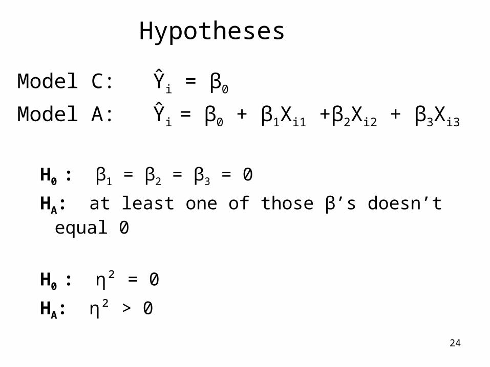
Hypotheses

Model C: Ŷi = β0

Model A: Ŷi = β0 + β1Xi1 +β2Xi2 + β3Xi3

H0 : β1 = β2 = β3 = 0

HA: at least one of those β’s doesn’t equal 0

H0 : η² = 0

HA: η² > 0

25

Insert SPSS Printout Here

26

Testing Statistical Significance

We will now go through the three (equivalent) ways of testing the statistical significance of Model A (just to make sure we understand them). SPSS gives us the p value for the ‘MS to F’ method, and says that p=.000, note that p will never actually equal zero, in this case it rounds to zero at three decimal places (so is pretty darn small). It would be preferable to say p<.0001. We can also use the F or PRE tools. Understand that the p value is the same no matter which of the three approaches we use.

27

Method 1: Testing the Significance of the PRE

PRE = .220 (from SPSS)

PREcritical (from PRE critical table)

N=414

PC=1

PA=4

N-PA=410

PA-PC=3

PREcritical between .038 and .015

28

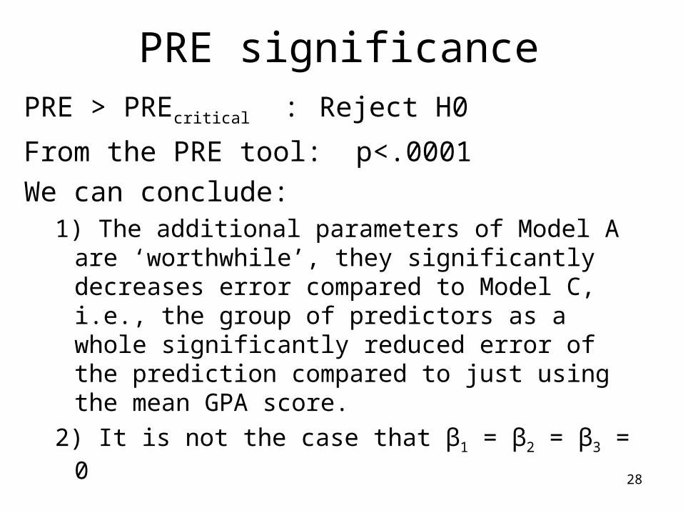
PRE significancePRE > PREcritical : Reject H0

From the PRE tool: p<.0001

We can conclude:1) The additional parameters of Model A are

‘worthwhile’, they significantly decreases error compared to Model C, i.e., the group of predictors as a whole significantly reduced error of the prediction compared to just using the mean GPA score.

2) It is not the case that β1 = β2 = β3 = 0

29

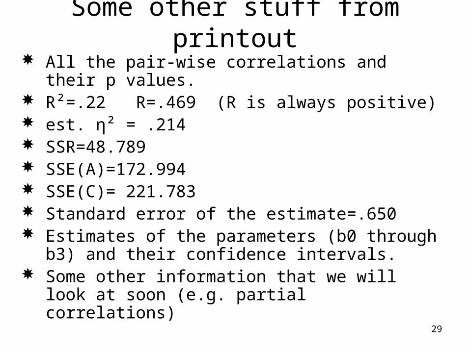
Some other stuff from printout All the pair-wise correlations and their p values. R²=.22 R=.469 (R is always positive) est. η² = .214 SSR=48.789 SSE(A)=172.994 SSE(C)= 221.783 Standard error of the estimate=.650 Estimates of the parameters (b0 through b3) and

their confidence intervals. Some other information that we will look at soon

(e.g. partial correlations)

30

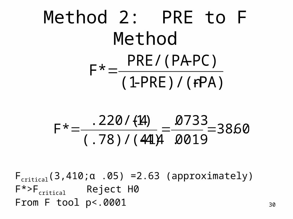
Method 2: PRE to F Method

PA)-PRE)/(n-(1

PC)-PRE/(PAF*

60.380019.

0733.

4)-(.78)/(414

1)-.220/(4F*

Fcritical(3,410;α .05) =2.63 (approximately)F*>Fcritical Reject H0From F tool p<.0001

31

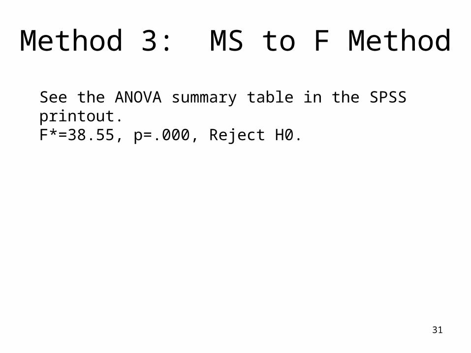
Method 3: MS to F Method

See the ANOVA summary table in the SPSS printout.F*=38.55, p=.000, Reject H0.

32

Problems with overall model test

1. If some of the parameters in A are worthwhile and some are not, the PRE per parameter added may not be very impressive, with the weaker parameters washing out the effects of the stronger.

2. As with the overall F test in ANOVA, our alternative hypothesis is very vague, that at least one β1 through βp-1 doesn’t equal 0. If Model A is worthwhile overall, we don’t know which of its individual parameters contributed to that worthwhileness.