1 Population Growth Models

Back to our problem of trying to predict the future, or at least the future population of somespecies in some region. Two ideas for how to do this come to mind.

The first is to look at the historical data and see if we can identify trends. This is agreat idea, but is often very difficult. Data seldom fits a simple pattern perfectly and wemust constantly worry about what trends are “real” in the data, what trends are due totemporary changes in the situation and what trends are created by our human desire to seepatterns, even when there are none.

The other idea is to try to make a deterministic model of the population that is basedon some basic assumptions of how the population changes. We need a model that is simpleenough to use, but complicated enough to give an at least approximately reliable predictions.

The first idea requires we be able to interpret data from a complicated noisy world so weneed techniques and expertise in statistics (stay tuned!). So for now we follow the secondidea and construct models based on some (simple) assumptions about biology. Of course,combining both model building and data analysis–using the data to motivate and check theassumptions and using the models to tease out trends in the data–is more powerful thaneither technique by itself.

Think of this section as practice building models for physical world and seeing what kindsof behavior simple models can predict. The “hidden” agenda is to use some of the functionswe have seen in our zoo.

1.1 Exponential Growth Models

As fits our basic outline, we start by making a simple, abstract model of the growth of apopulation. We are guided by a principle called “Occam’s Razor” which states that a model(or explanation) should be the simplest possible model that “works”. That is, we do notwant to add complication unless we must to match reality.

So, consider a small population of some species let loose in a large area. For example, inOctober 1859, Thomas Austin released 24 rabbits on his farm in Australia (at least accordingto Wikipedia). This population eventually grew to over 600 million.

We let t represent time measured in years. If we were considering a population of whaleswe might measure time in decades while for bacteria, we would measure time in hours orminutes. We let P (t) be the population at time t. Again, we might measure P as number ofindividuals (for whales), or thousands or millions of individuals (for rabbits or people). Wecould also let P represent a population density. That is, we could let P be the number ofrabbits per square kilometer or square meter. So fractional values of P are allowed.

As the notation suggests, we think of P (t) as a function of t. Our goal is to be able topredict a value of P (t) for any time t. We could just write down a guess for a formula ofP (t), but that isn’t much more satisfying than just guessing the values of P (t). Instead, let’sthink a (very) little bit about biology.

What do we know about rabbits? Well, rabbits do what they are famous for and begetmore rabbits. The more rabbits you have this year, the more baby rabbits you will havenext year. So the (very) basic biology of rabbits tells us not what the population of rabbitsis, but rather, how the population changes.

1

Our models for population size will be based on rules derived from how the populationchanges. Keeping with Occam’s Razor, we start with the simplest aspects of populationchange and make some explicit assumptions about how they work:

1. The number of births between time t and time t + 1 is proportional to the size of thepopulation P (t) at time t. That is, there is a constant b > 0 such that the number ofbirths between time t and t + 1 is b · P (t).

2. The number of deaths between time t and time t + 1 is also proportional to the size ofthe size of the population P (t) at time t. That is, there is a constant d > 0 such thatthe number of deaths between time t and t + 1 is d · P (t).

Clearly, these are just the most basic assumptions on how any population might change.There are many factors that effect births and deaths. These include external factors, likethe weather, and factors that depend on where the species is on the food chain. However,we start simple and ignore all other mechanisms of population change.

Now we must turn these assumptions into statements that we can use to compute fu-ture populations. While this makes our discussion look more “mathy”–formulas instead ofsentences–we emphasize that all we are doing in this step is translating the sentences aboveinto a form we can use for computation.

Putting our two assumptions together, we can say that the population at time t + 1 isthe population at time t plus the births between t and t+ 1 minus the deaths between t andt + 1. We can write this on one line as

Population at time t + 1 = (population at time t) + (births t to t + 1)− (deaths t to t + 1).

Now our assumptions say that the births time t to t + 1 are given by bP (t) while the deathsare given by dP (t). Hence, we can shorten the sentence above with notation, writing

P (t + 1) = P (t) + bP (t)− dP (t).

This completes our translation of the assumptions into a formula (and it really is only atranslation). We can now use the algebra you learned long ago to simplify things even more.By factoring out P (t) on the right, we get

P (t + 1) = (1 + b− d)P (t).

We can consolidate a bit more by letting

k = 1 + b− d

and calling k the “growth rate constant”. Our model can now be written in the very efficientform

P (t + 1) = kP (t).

If there are more births than deaths (b > d), then k > 1 and the population at time t+1is larger than the population at time t. If we know the population at time t = 0, then attime t = 1 we have

P (1) = kP (0)

2

and at time t = 2 we have

P (2) = kP (1) = k(kP (0)) = k2P (0)

and at time t = 3 we have

P (3) = kP (2) = k(k2P (0)) = k3P (0).

You can see the pattern developing here. A proof (by induction) shows the general case that

P (N) = kP (N − 1) = k(kN−1P (0)) = kNP (0)

and we have a formula for the population for all future times N– provided we know thepopulation at time zero.

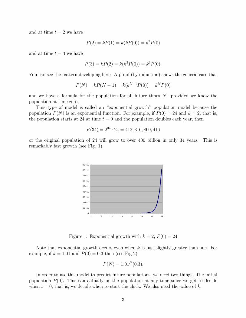
This type of model is called an “exponential growth” population model because thepopulation P (N) is an exponential function. For example, if P (0) = 24 and k = 2, that is,the population starts at 24 at time t = 0 and the population doubles each year, then

P (34) = 234 · 24 = 412, 316, 860, 416

or the original population of 24 will grow to over 400 billion in only 34 years. This isremarkably fast growth (see Fig. 1).

0

1E+11

2E+11

3E+11

4E+11

5E+11

6E+11

7E+11

8E+11

9E+11

0 5 10 15 20 25 30 35

Figure 1: Exponential growth with k = 2, P (0) = 24

Note that exponential growth occurs even when k is just slightly greater than one. Forexample, if k = 1.01 and P (0) = 0.3 then (see Fig 2)

P (N) = 1.01N(0.3).

In order to use this model to predict future populations, we need two things. The initialpopulation P (0). This can actually be the population at any time since we get to decidewhen t = 0, that is, we decide when to start the clock. We also need the value of k.

3

0

1000

2000

3000

4000

5000

6000

7000

0 100 200 300 400 500 600 700 800 900 1000 1100 1200

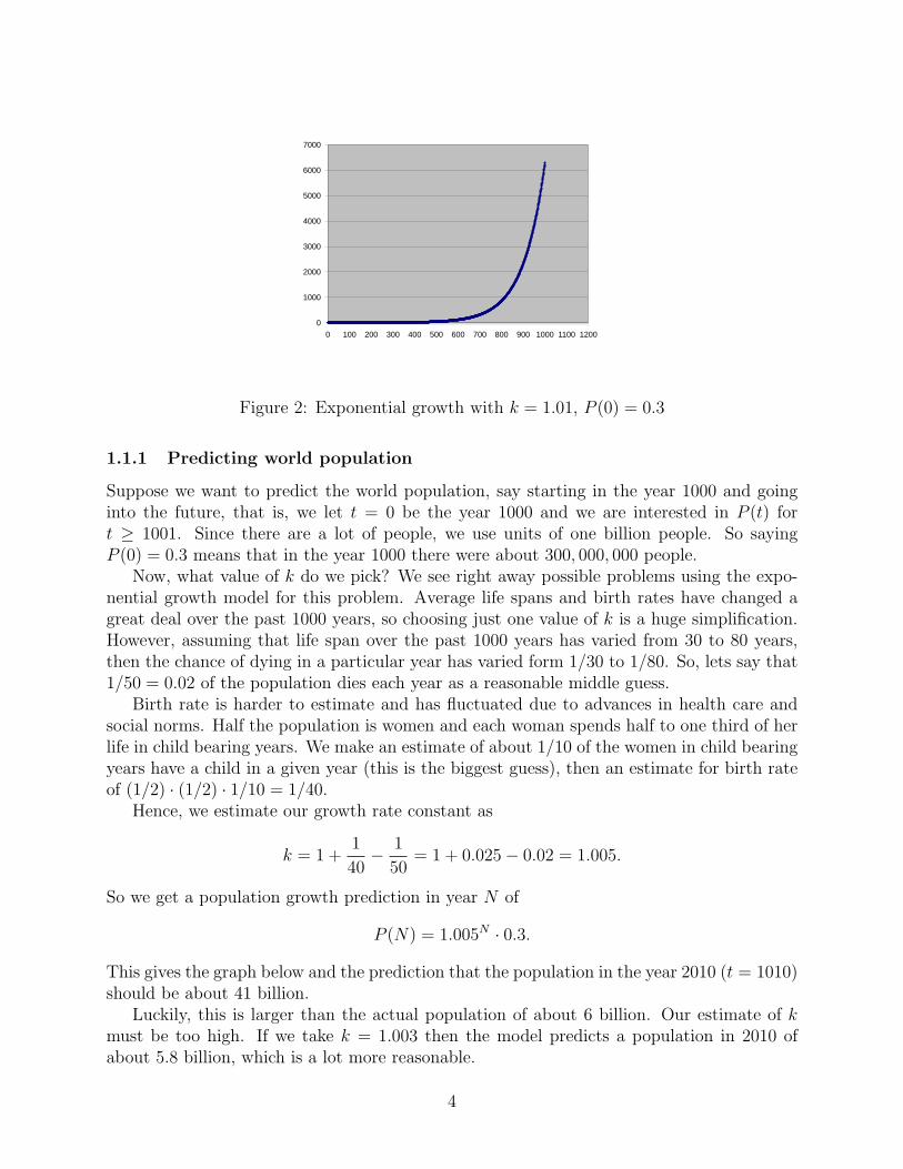
Figure 2: Exponential growth with k = 1.01, P (0) = 0.3

1.1.1 Predicting world population

Suppose we want to predict the world population, say starting in the year 1000 and goinginto the future, that is, we let t = 0 be the year 1000 and we are interested in P (t) fort ≥ 1001. Since there are a lot of people, we use units of one billion people. So sayingP (0) = 0.3 means that in the year 1000 there were about 300, 000, 000 people.

Now, what value of k do we pick? We see right away possible problems using the expo-nential growth model for this problem. Average life spans and birth rates have changed agreat deal over the past 1000 years, so choosing just one value of k is a huge simplification.However, assuming that life span over the past 1000 years has varied from 30 to 80 years,then the chance of dying in a particular year has varied form 1/30 to 1/80. So, lets say that1/50 = 0.02 of the population dies each year as a reasonable middle guess.

Birth rate is harder to estimate and has fluctuated due to advances in health care andsocial norms. Half the population is women and each woman spends half to one third of herlife in child bearing years. We make an estimate of about 1/10 of the women in child bearingyears have a child in a given year (this is the biggest guess), then an estimate for birth rateof (1/2) · (1/2) · 1/10 = 1/40.

Hence, we estimate our growth rate constant as

k = 1 +1

40− 1

50= 1 + 0.025− 0.02 = 1.005.

So we get a population growth prediction in year N of

P (N) = 1.005N · 0.3.

This gives the graph below and the prediction that the population in the year 2010 (t = 1010)should be about 41 billion.

Luckily, this is larger than the actual population of about 6 billion. Our estimate of kmust be too high. If we take k = 1.003 then the model predicts a population in 2010 ofabout 5.8 billion, which is a lot more reasonable.

4

0

5

10

15

20

25

30

35

40

45

50

0 100 200 300 400 500 600 700 800 900 1000 1100

Figure 3: Exponential growth with k = 1.005, P (0) = 0.3

0

1

2

3

4

5

6

7

0 100 200 300 400 500 600 700 800 900 1000 1100

Figure 4: Exponential growth with k = 1.003, P (0) = 0.3

1.2 Criticism of the Exponential Growth Model

As noted above, the use of a constant growth rate constant k is the most serious assumptionin this model. Obviously, improvements in public health, wars, changes in social attitudescan make a large difference in k.

This does not mean that the exponential growth model is useless–it just means that wehave to be careful where and how we use it. For the example above, it tells us that formost of the last thousand years, the growth rate constant must have been very small. Weare forced to re-examine our assumptions about birth and death rates. A small populationin a large environment under fairly constant conditions will probably follow an exponentialgrowth model fairly accurately, at least until the population becomes too large.

The moral is: There is no magic answer and no substitute for careful thought whenbuilding and evaluating models.

5

1.3 Another View of the Exponential Growth model

Before looking at more generally applicable population models, we need to use what we knowabout functions to get a different view of the exponential growth model.

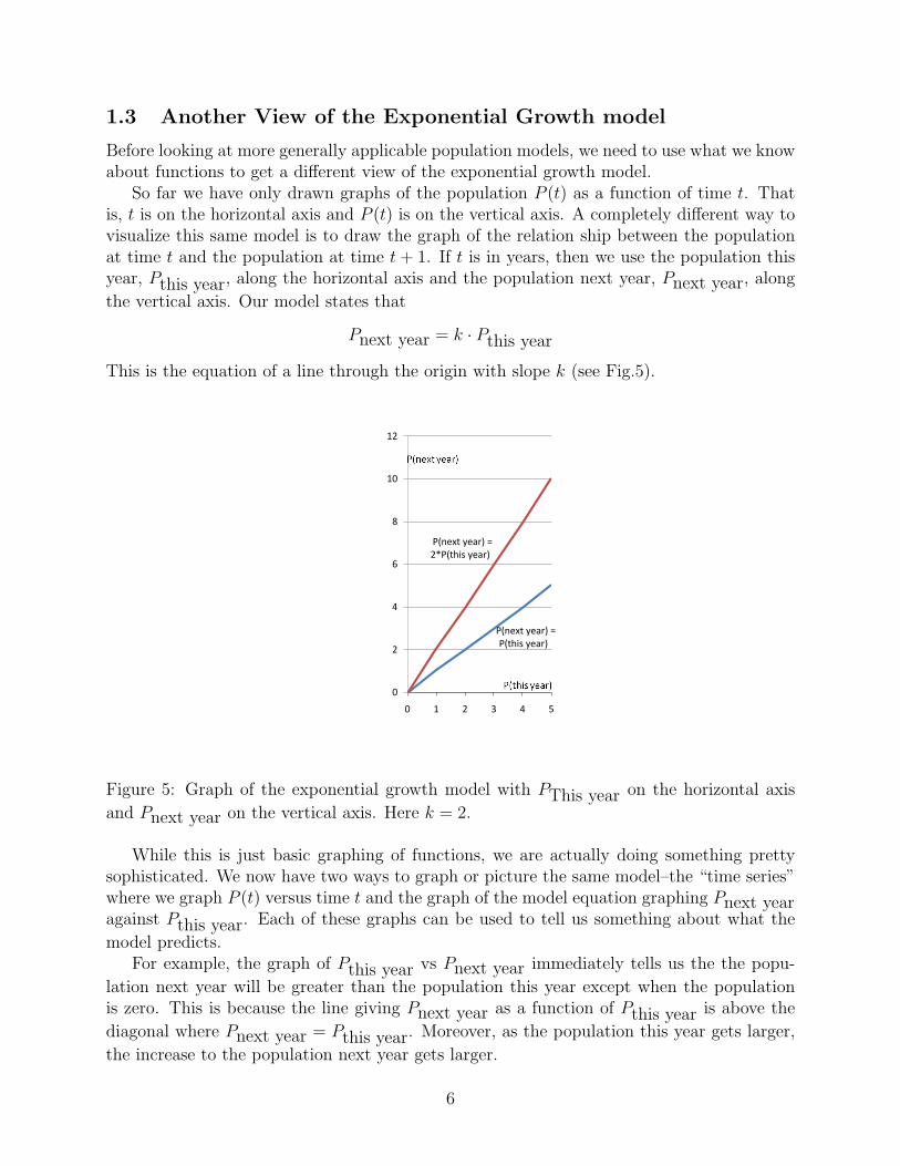
So far we have only drawn graphs of the population P (t) as a function of time t. Thatis, t is on the horizontal axis and P (t) is on the vertical axis. A completely different way tovisualize this same model is to draw the graph of the relation ship between the populationat time t and the population at time t + 1. If t is in years, then we use the population thisyear, Pthis year, along the horizontal axis and the population next year, Pnext year, along

the vertical axis. Our model states that

Pnext year = k · Pthis year

This is the equation of a line through the origin with slope k (see Fig.5).

0

2

4

6

8

10

12

0 1 2 3 4 5

P(next year) =P(this year)

P(next year) =2*P(this year)

Figure 5: Graph of the exponential growth model with PThis year on the horizontal axis

and Pnext year on the vertical axis. Here k = 2.

While this is just basic graphing of functions, we are actually doing something prettysophisticated. We now have two ways to graph or picture the same model–the “time series”where we graph P (t) versus time t and the graph of the model equation graphing Pnext yearagainst Pthis year. Each of these graphs can be used to tell us something about what the

model predicts.For example, the graph of Pthis year vs Pnext year immediately tells us the the popu-

lation next year will be greater than the population this year except when the populationis zero. This is because the line giving Pnext year as a function of Pthis year is above the

diagonal where Pnext year = Pthis year. Moreover, as the population this year gets larger,

the increase to the population next year gets larger.

6

Which of these two graphical representations of the model we use depends what we wantto learn about what the model predicts. It is like looking at the body of an elephant or theDNA of an elephant. They both give the same information, but in a very different forms. Ifwe want to see what the model predicts for the population far in the future for a particularinitial population P (0), then we look at the graph with time t on the horizontal axis andP (t) on the vertical axis. If we want to visualized the model directly, then we look at thegraph with the population this year on the horizontal axis and the population next year onthe vertical axis, which allows us to predict one year in the future for any P value. Beingable to move between these two pictures is a very useful skill which we study next.

2 Exponential Growth and Harvesting

The case of rabbits in Australia is one of the best known and one of the most dramatic casesof exponential growth of an introduced invasive species. Sadly, it is not the only case–otherexamples include cane toads in Australia, Kudzu in the southern U.S. and zebra muscles inthe midwestern U.S. (and recently in western Massachusetts).

What seems a harmless, or even beneficial species from another area of the world, canbecome a pest or weed very quickly when there are no natural controls on its populationgrowth. An example in the news lately is the Asian or silver carp which was imported tothe U.S. to clean commercial fish farm tanks. After their escape during a flood to the lowerMississippi, the carp has spread north and now is within six miles of entering the greatlakes. These carp eat plankton voraciously cutting off the food chain for native species.They also have the annoying habit of jumping out of the water when disturbed by boats.(You can find videos of this on youtube–search jumping asian carp. A more thoughtful videoon this invasive species is at http://www.youtube.com/watch?v=oii4U3cQx E ) Expect tohear more about this if (or when) they reach lake Michigan.

Once a species is recognized as a pest, attempts are made to control its growth. Typically,these include attempts to “harvest” the species, that is, remove as many as possible fromthe environment.

As our next model, we adjust the exponential growth model to add the effect of harvest-ing. This is an interesting and important topic both for controlling invasive species and formanaging useful wild populations, but we also have a hidden agenda. At the end of the lastsection we saw that there are two ways to “picture” the exponential growth model. Thatis, there are two different graphs that we can draw that contain all the information aboutthe model. They are the graph of the population as a function of time and the graph of thepopulation next year as a function of the population this year. In this section we study howthese two views of a model are related and how we can use both pictures to make predictionsabout the future from the model.

2.1 Model of Exponential Growth with Harvesting

We start with the same notation and assumptions we had in the last section. That is, tis time (which, for convenience, we say is measured in years), P (t) is the population attime t measured in some convenient units. For the exponential model, we assume that the

7

population only changes because of births and deaths and that the number of each of theseis proportional to the total size of the population. Our fundamental equation is

P (t + 1) = kP (t)

orPnext year = kPthis year

where k is the growth rate constant. As long as k > 1, and the initial population P (0) isbigger than zero, the population will grow exponentially,

P (N) = kNP (0).

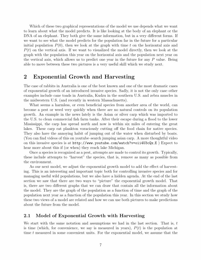
We picture this below for k = 1.5. Fig. 6 is the graph of the population next year as a functionof the population this year. Fig. 7is a typical graph of the growth of a particular populationwhere P (0) is chosen to be 0.3 (so here we are measuring P in thousands or millions ofindividuals or by density, individuals per square kilometer, so that decimal numbers forpopulation make sense). Note that to produce Fig. 7 we need to specify both k and P (0)–this graph changes if P (0) is adjusted.

0

0.2

0.4

0.6

0.8

1

1.2

1.4

1.6

0 0.2 0.4 0.6 0.8 1

P(next year) =P(this year)

P(next year) =1.5*P(this year)

Figure 6: Graph of the exponential growth model with PThis year on the horizontal axis

and Pnext year on the vertical axis. Here k = 1.5.

Now we add the effect “harvesting” to the exponential model. By harvesting we meanthe removal of members of the population. The simplest way to manage a useful populationis to give out a certain predetermined number of licenses (hunting licenses or catch limitsfor fishing or permits for logging, etc.) When trying to eliminate a pest or weed population,as many individuals as possible are removed and the limiting factor is the amount of money

8

0

200

400

600

800

1000

1200

0 2 4 6 8 10 12 14 16 18 20

Figure 7: Graph of the exponential growth model with time t on the horizontal axis andpopulation P (t) on the vertical axis. Here k = 1.5 and the initial population is P (0) = 0.3.

available. In either case, we assume that the number of individuals removed each year is aconstant which we call H. Also, for simplicity, we assume H remains constant from year toyear.

Our new model can now be written

Pnext year = kPthis year −H.

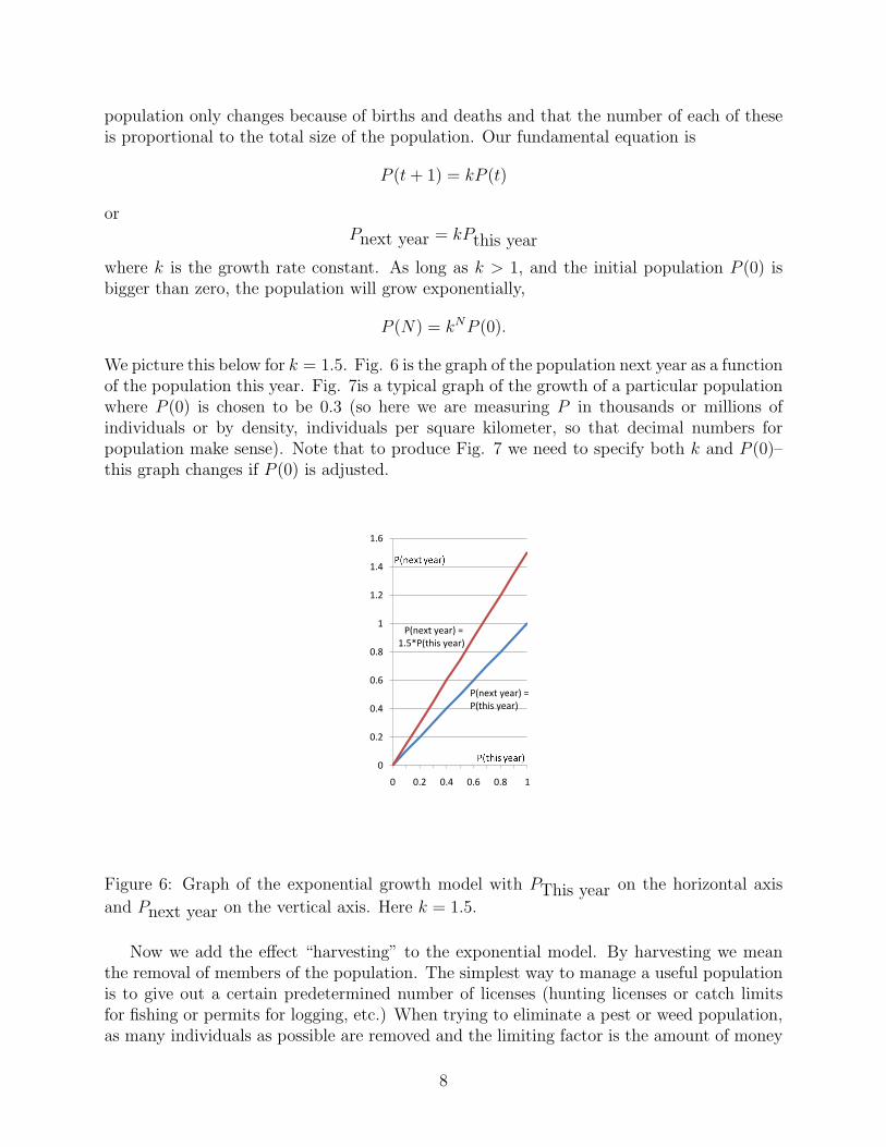
We are assuming that the harvesting does not effect the growth rate constant k (individuals ofthe species reproduce just as effectively as before), so the only change in the new populationmodel is the −H term. To see how this changes things, let’s pick particular numbers. Sayk = 1.5 as above and let’s take H = 0.2 and graph the population next year as a function ofthe population this year (see Fig. 8).Note that the only difference between Fig.8 and Fig. 6 for the exponential model, is that theline is pushed down. The “vertical intercept” is now at −0.2, while the slope k, the same asabove.

2.2 What Does This Model Predict?

Taking k = 1.5 and H = 0.2, we compare the predictions of the exponential growth model,

Pnext year = 1.5Pthis year

to the exponential growth with harvesting model,

Pnext year = 1.5Pthis year − 0.2,

using the same initial populations. If we start with P (0) = 0.3, then for the exponentialgrowth model, we have already seen that

P (N) = 1.5N0.3.

9

-0.4

-0.2

0

0.2

0.4

0.6

0.8

1

1.2

1.4

0 0.2 0.4 0.6 0.8 1

P(next year)=P(this year)

P(next year) =1.5*P(this year)-0.2

Figure 8: Graph of the exponential model with harvesting with k = 1.5 and H = 0.2, alongwith the diagonal.

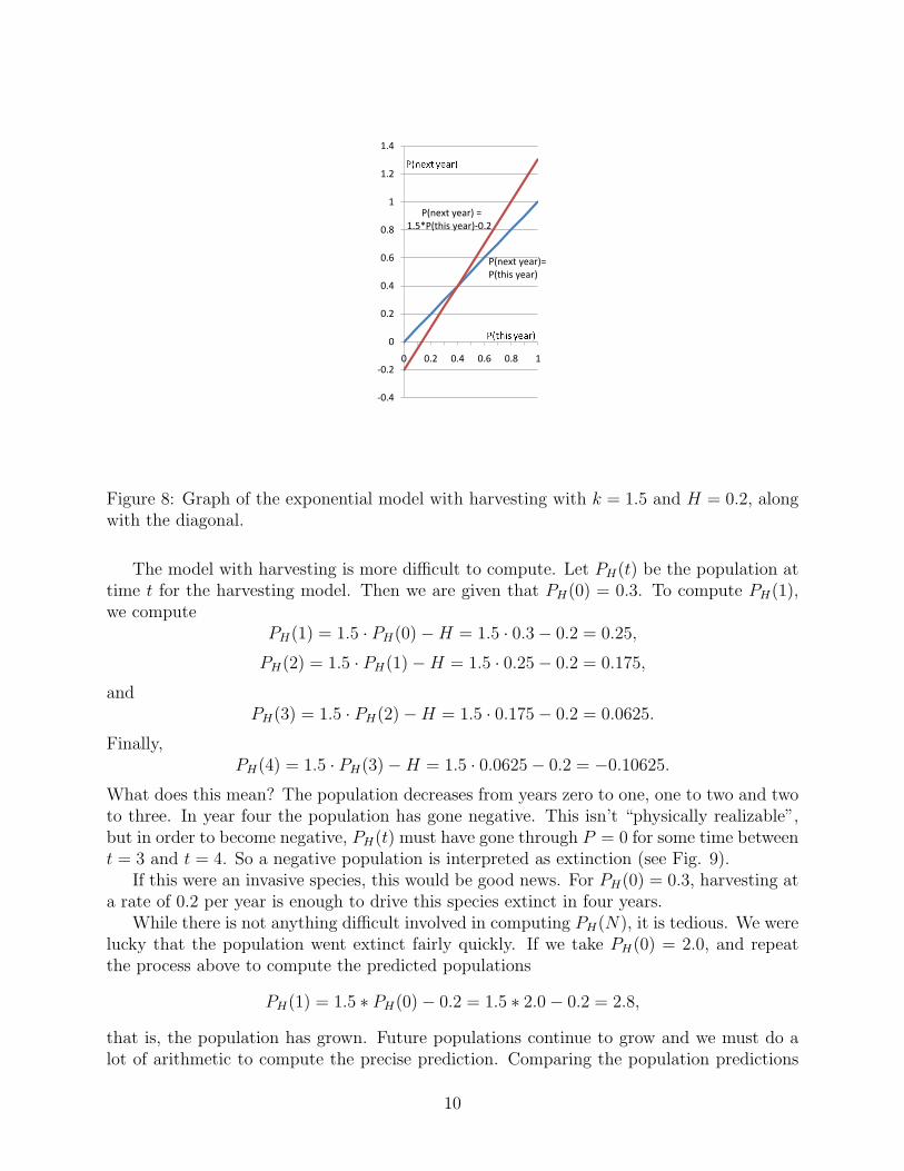
The model with harvesting is more difficult to compute. Let PH(t) be the population attime t for the harvesting model. Then we are given that PH(0) = 0.3. To compute PH(1),we compute

PH(1) = 1.5 · PH(0)−H = 1.5 · 0.3− 0.2 = 0.25,

PH(2) = 1.5 · PH(1)−H = 1.5 · 0.25− 0.2 = 0.175,

andPH(3) = 1.5 · PH(2)−H = 1.5 · 0.175− 0.2 = 0.0625.

Finally,PH(4) = 1.5 · PH(3)−H = 1.5 · 0.0625− 0.2 = −0.10625.

What does this mean? The population decreases from years zero to one, one to two and twoto three. In year four the population has gone negative. This isn’t “physically realizable”,but in order to become negative, PH(t) must have gone through P = 0 for some time betweent = 3 and t = 4. So a negative population is interpreted as extinction (see Fig. 9).

If this were an invasive species, this would be good news. For PH(0) = 0.3, harvesting ata rate of 0.2 per year is enough to drive this species extinct in four years.

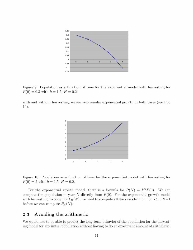
While there is not anything difficult involved in computing PH(N), it is tedious. We werelucky that the population went extinct fairly quickly. If we take PH(0) = 2.0, and repeatthe process above to compute the predicted populations

PH(1) = 1.5 ∗ PH(0)− 0.2 = 1.5 ∗ 2.0− 0.2 = 2.8,

that is, the population has grown. Future populations continue to grow and we must do alot of arithmetic to compute the precise prediction. Comparing the population predictions

10

-0.15

-0.1

-0.05

0

0.05

0.1

0.15

0.2

0.25

0.3

0.35

0 1 2 3 4

Figure 9: Population as a function of time for the exponential model with harvesting forP (0) = 0.3 with k = 1.5, H = 0.2.

with and without harvesting, we see very similar exponential growth in both cases (see Fig.10).

0

1

2

3

4

5

6

7

8

9

0 1 2 3 4

Figure 10: Population as a function of time for the exponential model with harvesting forP (0) = 2 with k = 1.5, H = 0.2.

For the exponential growth model, there is a formula for P (N) = kNP (0). We cancompute the population in year N directly from P (0). For the exponential growth modelwith harvesting, to compute PH(N), we need to compute all the years from t = 0 to t = N−1before we can compute PH(N).

2.3 Avoiding the arithmetic

We would like to be able to predict the long-term behavior of the population for the harvest-ing model for any initial population without having to do an exorbitant amount of arithmetic.

11

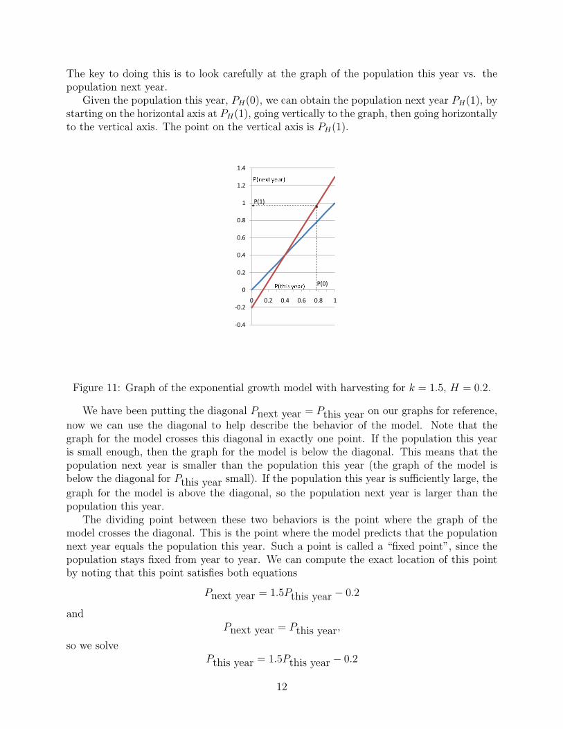
The key to doing this is to look carefully at the graph of the population this year vs. thepopulation next year.

Given the population this year, PH(0), we can obtain the population next year PH(1), bystarting on the horizontal axis at PH(1), going vertically to the graph, then going horizontallyto the vertical axis. The point on the vertical axis is PH(1).

-0.4

-0.2

0

0.2

0.4

0.6

0.8

1

1.2

1.4

0 0.2 0.4 0.6 0.8 1

P(1)

P(0)

Figure 11: Graph of the exponential growth model with harvesting for k = 1.5, H = 0.2.

We have been putting the diagonal Pnext year = Pthis year on our graphs for reference,

now we can use the diagonal to help describe the behavior of the model. Note that thegraph for the model crosses this diagonal in exactly one point. If the population this yearis small enough, then the graph for the model is below the diagonal. This means that thepopulation next year is smaller than the population this year (the graph of the model isbelow the diagonal for Pthis year small). If the population this year is sufficiently large, the

graph for the model is above the diagonal, so the population next year is larger than thepopulation this year.

The dividing point between these two behaviors is the point where the graph of themodel crosses the diagonal. This is the point where the model predicts that the populationnext year equals the population this year. Such a point is called a “fixed point”, since thepopulation stays fixed from year to year. We can compute the exact location of this pointby noting that this point satisfies both equations

Pnext year = 1.5Pthis year − 0.2

andPnext year = Pthis year,

so we solvePthis year = 1.5Pthis year − 0.2

12

for Pthis year. This occurs at P = 0.4. So if PH(0) < 0.4 then the population dies out, but

if PH(0) > 0.4 then the population grows. Eventually, it grows like the exponential growthmodel

2.4 Types of functions

The exponential growth model with harvesting gives us a new view of what kinds of functionscan occur by using models and gives us two different ways to look at the same model. ForH = 0, that is, just the exponential growth model, every non-zero initial condition leads toa rapidly growing population.

For H > 0, and PH(0) sufficiently large, the model still predicts a rapidly growingpopulation.

However, for H > 0 and a small initial population (PH(0) close to zero), the modelpredicts a population that quickly crashes to extinction.

Finally, for each value of H > 0, the exponential growth model with harvesting predictsthe existence of a fixed point–that is, the model predicts a population where harvesting anddeaths are exactly balanced by births, so the population stays the same from year to year.In this case the graph of the population as a function of time is just a constant function.

2.5 The power of a clever idea

Again we see that the power of mathematics comes not in massively complicated equationsor hugely elaborate arithmetic. The great ideas in mathematics come when somebody looksat some problem in a new way. The idea of looking at a model by graphing the populationthis year vs the population next year does not require hard computations, so far our graphshave been lines. However, the idea of drawing this picture and using it to say things aboutwhat the model predicts for different initial populations is very useful. We exploit this ideain the next section.

While the problems of population biology can be both very interesting and extremelyimportant (ask anyone who has been knocked out of their boat by a large silver carp),don’t forget the bigger picture. We are following the process of modelling–making a model,learning things about the model, then refining the model to do a better job reflecting thesituation of the original problem.

3 Limited growth

We know that growth, particularly exponential growth, can not go on forever in a finiteenvironment. For populations with the ability to spread widely (like people) we forget thisbecause the earth is very big and we are relatively small. However, eventually, growth mustsubside–you just run out of room.

Situations where the limits to growth effect the sizes of populations are not hard tofind. Populations restricted to small islands, species whose biology restrict them to thehigh altitudes of mountain peaks and plants and animals in isolated ponds face these limitsrelatively quickly. For example, on Lovells and Gallops islands in Boston Harbor, it is hard

13

to walk down a path without encountering a large fluffy rabbit. (By the way, this is a lovelyday trip when it gets warmer.) These populations are large for the size of the islands andthe dynamics of the population is very interesting.

3.1 A model incorporating a limit to growth

To modify the exponential model so that growth does not continue forever, we make thefollowing assumptions

1. The exponential growth model works well for small populations.

2. There is some population size, call it C, such that if the population ever gets to C orabove then all the resources are consumed and the next time period the population iszero.

The new parameter C is the absolute upper bound to growth. We will call C the “crashpopulation”. If the population reaches C, then the population immediately goes extinct.Presumedly, a population near C would consume almost all the resources, so there would bemany more deaths than births and the population would crash to close to zero.

There are many ways to build a model that satisfies these assumptions, but we rememberOccum’s Razor and try to find a simple model. There are two ways to proceed. First wecould try algebra. Since the assumption says that exponential growth is a good model forsmall populations, our model should look like

Pnext year = kPthis year

when Pthis year is small. However, when Pthis year is C then Pnext year is zero. We

can include this in the model by multiplying on the right by a term which is zero whenPthis year = C, for example,

Pnext year = kPthis year

(1−

Pthis year

C

).

Note if Pthis year is near zero, then (1− Pthis year/C) is near one so the model is near the

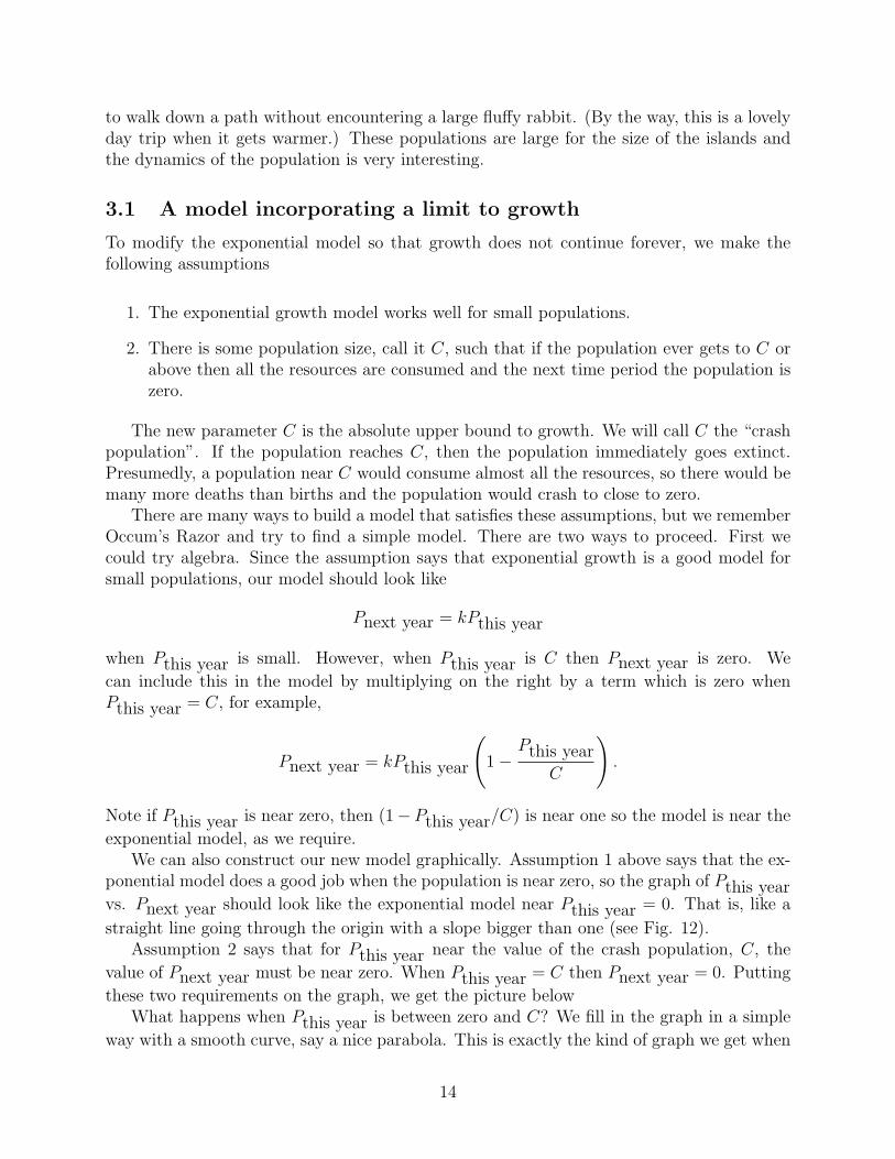
exponential model, as we require.We can also construct our new model graphically. Assumption 1 above says that the ex-

ponential model does a good job when the population is near zero, so the graph of Pthis yearvs. Pnext year should look like the exponential model near Pthis year = 0. That is, like a

straight line going through the origin with a slope bigger than one (see Fig. 12).Assumption 2 says that for Pthis year near the value of the crash population, C, the

value of Pnext year must be near zero. When Pthis year = C then Pnext year = 0. Putting

these two requirements on the graph, we get the picture belowWhat happens when Pthis year is between zero and C? We fill in the graph in a simple

way with a smooth curve, say a nice parabola. This is exactly the kind of graph we get when

14

0

0.5

1

1.5

2

2.5

3

3.5

4

4.5

0 0.5 1 1.5 2 2.5 3 3.5 4

SmoothConnection

Assumption 1 Assumption 2

Figure 12: Building the limited growth model from the two assumptions.

we plot the function

Pnext year = kPthis year

(1−

Pthis year

C

).

This model is called the “Discrete Logistic model” of population growth in a limited envi-ronment. Since negative populations don’t make any sense, we usually add the requirementthat for Pthis year larger than C, the population next year is zero (i.e., extinct).

3.2 What does this model predict?

To see what kinds of population dynamics this model predicts, we look at some specificexamples. Suppose we are counting the population of thousands of rabbits on a small island.So we will count rabbits in units of 1000, i.e., P = 1 means a population of 1000 rabbits,etc.

Suppose for this island, the crash population (the population at which the rabbits eateverything an immediately go extinct) is 4000, or C = 4. If Pthis year is 4 or larger, then

next year the population will be extinct (Pnext year = 0).We try a number of different values of the growth rate constant k.

3.2.1 Small k

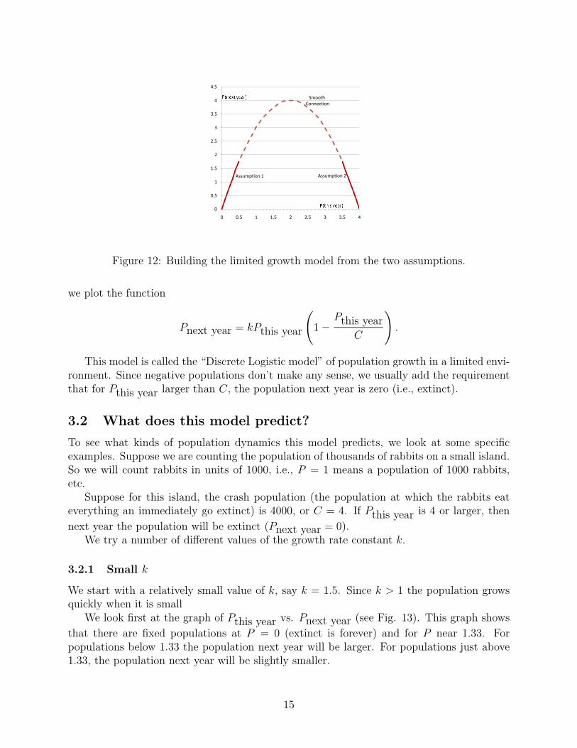
We start with a relatively small value of k, say k = 1.5. Since k > 1 the population growsquickly when it is small

We look first at the graph of Pthis year vs. Pnext year (see Fig. 13). This graph shows

that there are fixed populations at P = 0 (extinct is forever) and for P near 1.33. Forpopulations below 1.33 the population next year will be larger. For populations just above1.33, the population next year will be slightly smaller.

15

0

0.5

1

1.5

2

2.5

3

3.5

4

4.5

0 0.5 1 1.5 2 2.5 3 3.5 4

P(next year) =P(this year)

Figure 13: Graph of the Discrete Logistic model for k = 1.5.

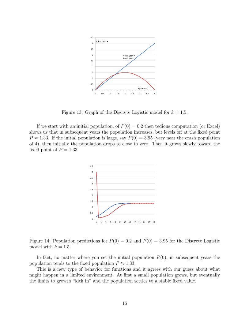
If we start with an initial population, of P (0) = 0.2 then tedious computation (or Excel)shows us that in subsequent years the population increases, but levels off at the fixed pointP ≈ 1.33. If the initial population is large, say P (0) = 3.95 (very near the crash populationof 4), then initially the population drops to close to zero. Then it grows slowly toward thefixed point of P = 1.33

0

0.5

1

1.5

2

2.5

3

3.5

4

4.5

1 3 5 7 9 11 13 15 17 19 21 23 25

Figure 14: Population predictions for P (0) = 0.2 and P (0) = 3.95 for the Discrete Logisticmodel with k = 1.5.

In fact, no matter where you set the initial population P (0), in subsequent years thepopulation tends to the fixed population P ≈ 1.33.

This is a new type of behavior for functions and it agrees with our guess about whatmight happen in a limited environment. At first a small population grows, but eventuallythe limits to growth “kick in” and the population settles to a stable fixed value.

16

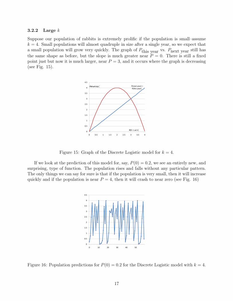
3.2.2 Large k

Suppose our population of rabbits is extremely prolific if the population is small–assumek = 4. Small populations will almost quadruple in size after a single year, so we expect thata small population will grow very quickly. The graph of Pthis year vs. Pnext year still has

the same shape as before, but the slope is much greater near P = 0. There is still a fixedpoint just but now it is much larger, near P = 3, and it occurs where the graph is decreasing(see Fig. 15).

0

0.5

1

1.5

2

2.5

3

3.5

4

4.5

0 0.5 1 1.5 2 2.5 3 3.5 4

P(next year) =P(this year)

Figure 15: Graph of the Discrete Logistic model for k = 4.

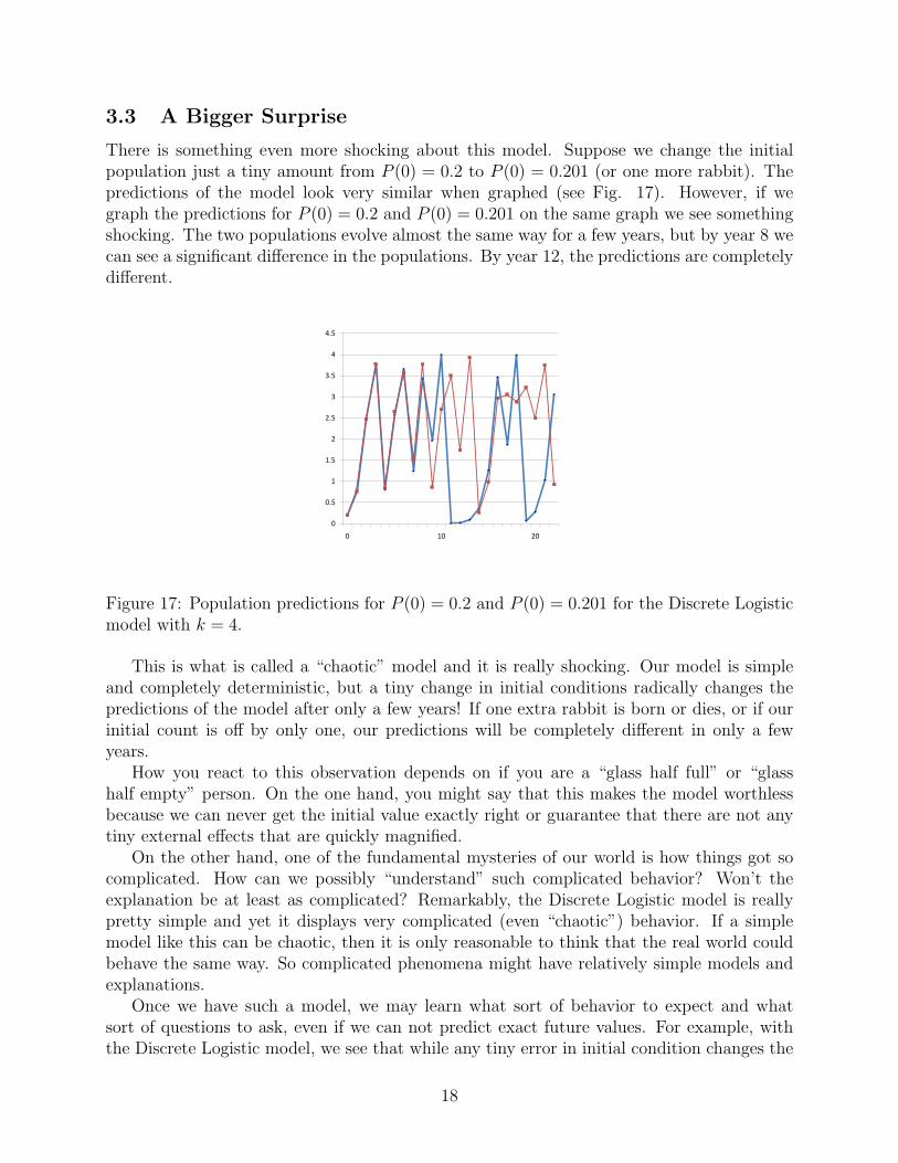
If we look at the prediction of this model for, say, P (0) = 0.2, we see an entirely new, andsurprising, type of function. The population rises and falls without any particular pattern.The only things we can say for sure is that if the population is very small, then it will increasequickly and if the population is near P = 4, then it will crash to near zero (see Fig. 16)

0

0.5

1

1.5

2

2.5

3

3.5

4

4.5

0 10 20 30 40 50

Figure 16: Population predictions for P (0) = 0.2 for the Discrete Logistic model with k = 4.

17

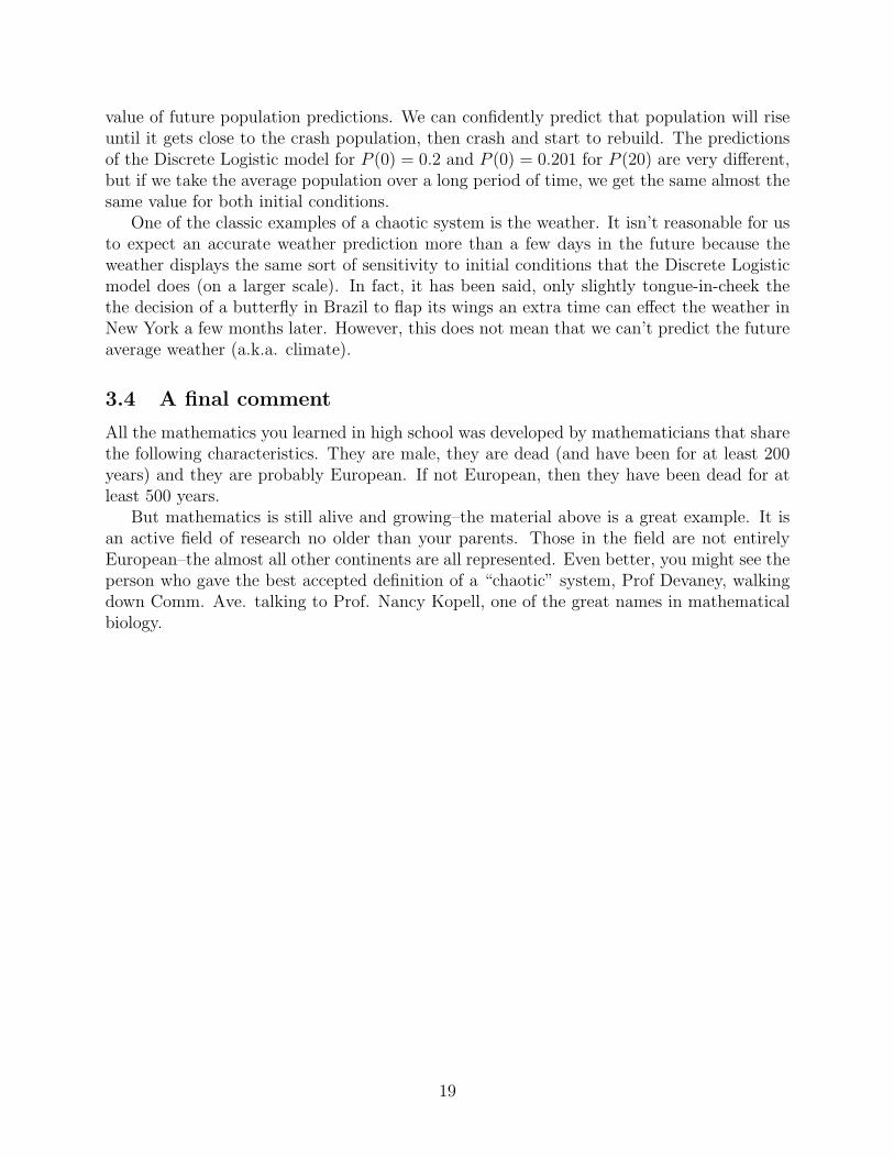
3.3 A Bigger Surprise

There is something even more shocking about this model. Suppose we change the initialpopulation just a tiny amount from P (0) = 0.2 to P (0) = 0.201 (or one more rabbit). Thepredictions of the model look very similar when graphed (see Fig. 17). However, if wegraph the predictions for P (0) = 0.2 and P (0) = 0.201 on the same graph we see somethingshocking. The two populations evolve almost the same way for a few years, but by year 8 wecan see a significant difference in the populations. By year 12, the predictions are completelydifferent.

0

0.5

1

1.5

2

2.5

3

3.5

4

4.5

0 10 20

Figure 17: Population predictions for P (0) = 0.2 and P (0) = 0.201 for the Discrete Logisticmodel with k = 4.

This is what is called a “chaotic” model and it is really shocking. Our model is simpleand completely deterministic, but a tiny change in initial conditions radically changes thepredictions of the model after only a few years! If one extra rabbit is born or dies, or if ourinitial count is off by only one, our predictions will be completely different in only a fewyears.

How you react to this observation depends on if you are a “glass half full” or “glasshalf empty” person. On the one hand, you might say that this makes the model worthlessbecause we can never get the initial value exactly right or guarantee that there are not anytiny external effects that are quickly magnified.

On the other hand, one of the fundamental mysteries of our world is how things got socomplicated. How can we possibly “understand” such complicated behavior? Won’t theexplanation be at least as complicated? Remarkably, the Discrete Logistic model is reallypretty simple and yet it displays very complicated (even “chaotic”) behavior. If a simplemodel like this can be chaotic, then it is only reasonable to think that the real world couldbehave the same way. So complicated phenomena might have relatively simple models andexplanations.

Once we have such a model, we may learn what sort of behavior to expect and whatsort of questions to ask, even if we can not predict exact future values. For example, withthe Discrete Logistic model, we see that while any tiny error in initial condition changes the

18

value of future population predictions. We can confidently predict that population will riseuntil it gets close to the crash population, then crash and start to rebuild. The predictionsof the Discrete Logistic model for P (0) = 0.2 and P (0) = 0.201 for P (20) are very different,but if we take the average population over a long period of time, we get the same almost thesame value for both initial conditions.

One of the classic examples of a chaotic system is the weather. It isn’t reasonable for usto expect an accurate weather prediction more than a few days in the future because theweather displays the same sort of sensitivity to initial conditions that the Discrete Logisticmodel does (on a larger scale). In fact, it has been said, only slightly tongue-in-cheek thethe decision of a butterfly in Brazil to flap its wings an extra time can effect the weather inNew York a few months later. However, this does not mean that we can’t predict the futureaverage weather (a.k.a. climate).

3.4 A final comment

All the mathematics you learned in high school was developed by mathematicians that sharethe following characteristics. They are male, they are dead (and have been for at least 200years) and they are probably European. If not European, then they have been dead for atleast 500 years.

But mathematics is still alive and growing–the material above is a great example. It isan active field of research no older than your parents. Those in the field are not entirelyEuropean–the almost all other continents are all represented. Even better, you might see theperson who gave the best accepted definition of a “chaotic” system, Prof Devaney, walkingdown Comm. Ave. talking to Prof. Nancy Kopell, one of the great names in mathematicalbiology.

19