1 Planning (under complete Knowledge) Intro to Artificial Intelligence.

1

Planning

(under complete Knowledge)

Intro to Artificial Intelligence

Why Planning Intelligent agents must operate in the world.

They are not simply passive reasoners (Knowledge Representation, reasoning under uncertainty) or problem solvers (Search), they must also act on the world.

We want intelligent agents to act in “intelligent ways”. Taking purposeful actions, predicting the expected effect of such actions, composing actions together to achieve complex goals.

2

Why Planning E.g. if we have a robot we want robot to

decide what to do; how to act to achieve our goals

3

A Planning Problem How to change the world to suit our needs Critical issue: we need to reason about what

the world will be like after doing a few actions, not just what it is like now

4

GOAL: Craig has coffeeCURRENTLY: robot in mailroom, has no coffee, coffee not made, Craig in office, etc.TO DO: goto lounge, make coffee,…

Planning Reasoning about what the world will be like after

doing a few actions is similar to what we have already examined.

However, now we want to reason about dynamic environments.

in(robby,Room1), lightOn(Room1) are true: will they be true after robby performs the action turnOffLights?

in(robby,Room1) is true: what does robby need to do to make in(robby,Room3) true?

Reasoning about the effects of actions, and computing what actions can achieve certain effects is at the heart of decision making.

5

Planning under Uncertainty One of the major complexities in planning that

we will deal with later is planning under uncertainty.

Our knowledge of the world probabilistic. Sensing is subject to noise (especially in

robots). Actions and effectors are also subject to error

(uncertainty in their effects).

6

Planning But for now we will confine our attention to

the deterministic case. We will examine:

Determining the effects of actions. finding sequences of actions that can achieve a

desired set of effects. This will in some ways be a lot like search, but we will

see that representation also plays an important role.

7

Situation Calculus First we look at how to model dynamic worlds

within first-order logic. The situation calculus is an important

formalism developed for this purpose. Situation Calculus is a first-order language. Include in the domain of individuals a special

set of objects called situations. Of these s0 is a special distinguished constant which denotes the “initial” situation.

8

Situation Calculus Situations are used to index “states” of the

world. When dealing with dynamic environments, the world has different properties at different points in time.

e.g., in(robby,room1, s0), in(robby,room3,s0) in(robby,room3,s1), in(robby,room1,s1).

Different things are true in situation s1 than in the initial situation s0.

Contrast this with the previous kinds of knowledge we examined.

9

Fluents The basic idea is that properties that change

from situation to situation (called fluents) take an extra situation argument.

clear(b) clear(b,s) “clear(b)” is no longer statically true, it is true

contingent on what situation we are talking about

10

Blocks World Example.clear(c,s0)

on(c,a,s0)

clear(b,s0)

handempty(s0)

11

C

A B

robothand

Actions in the Situation Calculus Actions are also part of language

A set of “primitive” action objects in the (semantic) domain of individuals.

In the syntax they are represented as functions mapping objects to primitive action objects.

pickup(X) function mapping blocks to actions pickup(c) = “the primitive action object corresponding

to ‘picking up block c’ stack(X,Y)

stack(a,b) = “the primitive action object corresponding to ‘stacking a on top of b’

12

Actions modify situations. There is a “generic” action application

function do(A,S). do maps a primitive action and a situation to a new situation.

The new situation is the situation that results from applying A to S.

do(pickup(c), s0) = the new situation that is the result of applying action “pickup(c)” to the initial situation s0.

13

What do Actions do? Actions affect the situation by changing what

is true. on(c,a,s0); clear(a,do(pickup(c),s0))

We want to represent the effects of actions, this is done in the situation calculus with two components.

14

Specifying the effects of actions Action preconditions. Certain things must hold

for actions to have a predictable effect. pickup(c) this action is only applicable to

situations S where “clear(c,S) handempty(S)” are true.

Action effects. Actions make certain things true and certain things false.

holding(c, do(pickup(c), S)) X.handempty(do(pickup(X),S))

15

Specifying the effects of actions Action effects are conditional on their

precondition being true.

S,X. ontable(X,S) clear(X,S) handempty(S) holding(X, do(pickup(X),S)) handempty(do(pickup(X),S)) ontable(X,do(pickup(X,S)) clear(X,do(pickup(X,S)).

16

Reasoning with the Situation Calculus.1. clear(c,s0)

2. on(c,a,s0)

3. clear(b,s0)

4. ontable(a,s0)

5. ontable(b,s0)

6. handempty(s0)

Query:Z.holding(b,Z)7. (holding(b,Z), ans(Z))

does there exists a situation in which we are holding b? And if so what is the name of that situation.

17

C

A B

Resolution Convert “pickup” action axiom into clause form:S,Y.

ontable(Y,S) clear(Y,S) handempty(S) holding(Y, do(pickup(Y),S)) handempty(do(pickup(Y),S)) ontable(Y,do(pickup(Y,S)) clear(Y,do(pickup(Y,S)).

8. (ontable(Y,S), clear(Y,S), handempty(S), holding(Y,do(pickup(Y),S))

9. (ontable(Y,S), clear(Y,S), handempty(S), handempty(do(pickup(X),S)))

10. (ontable(Y,S), clear(Y,S), handempty(S), ontable(Y,do(pickup(Y,S)))

11. (ontable(Y,S), clear(Y,S), handempty(S), clear(Y,do(pickup(Y,S)))

18

Resolution12. R[8d, 7]{Y=b,Z=do(pickup(b),S)}

(ontable(b,S), clear(b,S), handempty(S), ans(do(pickup(b),S)))

13. R[12a,5] {S=s0} (clear(b,s0), handempty(s0), ans(do(pickup(b),s0)))

14. R[13a,3] {}(handempty(s0), ans(do(pickup(b),s0)))

15. R[14a,6] {}ans(do(pickup(b),s0))

19

The answer? ans(do(pickup(b),s0)) This says that a situation in which you are

holding b is called “do(pickup(b),s0)”

This name is informative: it tells you what actions to execute to achieve “holding(b)”.

20

Two types of reasoning. In general we can answer questions of the

form: on(b,c,do(stack(b,c), do(pickup(b), s0)))

S. on(b,c,S) on(c,a,S)

The first involves predicting the effects of a sequence of actions, the second involves computing a sequence of actions that can achieve a goal condition.

21

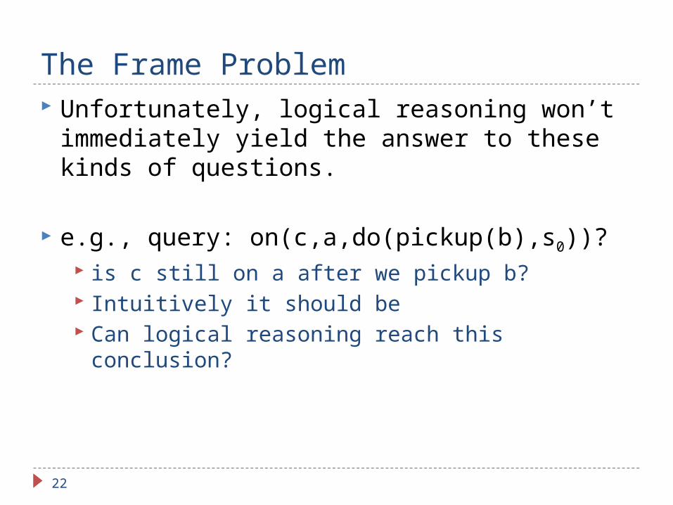
The Frame Problem Unfortunately, logical reasoning won’t

immediately yield the answer to these kinds of questions.

e.g., query: on(c,a,do(pickup(b),s0))? is c still on a after we pickup b? Intuitively it should be Can logical reasoning reach this conclusion?

22

The Frame Problem1. clear(c,s0)2. on(c,a,s0)3. clear(b,s0)4. ontable(a,s0)5. ontable(b,s0)6. handempty(s0)8. (ontable(Y,S), clear(Y,S), handempty(S),

holding(Y,do(pickup(Y),S))9. (ontable(Y,S), clear(Y,S), handempty(S),

handempty(do(pickup(X),S)))10. (ontable(Y,S), clear(Y,S), handempty(S),

ontable(Y,do(pickup(Y,S)))11. (ontable(Y,S), clear(Y,S), handempty(S),

clear(Y,do(pickup(Y,S)))12. on(c,a,do(pickup(b),s0)) {QUERY)

Nothing can resolve with 12!

23

Logical Consequence Remember that resolution only computes logical

consequences. We stated the effects of pickup(b), but did not

state that it doesn’t affect on(c,a). Hence there are models in which on(c,a) no longer

holds after pickup(b) (as well as models where it does hold).

The problem is that representing the non-effects of actions very tedious and in general is not possible.

Think of all of the things that pickup(b) does not affect!

24

The Frame Problem Finding an effective way of specifying the non-

effects of actions, without having to explicitly write them all down is the frame problem.

Very good solutions have been proposed, and the situation calculus has been a very powerful way of dealing with dynamic worlds:

logic based high level robotic programming languages

25

Computation Problems Although the situation calculus is a very

powerful representation. It is not always efficient enough to use to compute sequences of actions.

The problem of computing a sequence of actions to achieve a goal is “planning”

Next we will study some less rich representations which support more efficient planning.

26

CWA “ Classical Planning”. No incomplete or

uncertain knowledge. Use the “Closed World Assumption” in our

knowledge representation and reasoning. The Knowledge base used to represent a state of the

world is a list of positive ground atomic facts. CWA is the assumption that

if a ground atomic fact is not in our list of “known” facts, its negation must be true.

the constants mentioned in KB are all the domain objects.

27

CWA CWA makes our knowledge base much like a

database: if employed(John,CIBC) is not in the database, we conclude that employed(John, CIBC) is true.

28

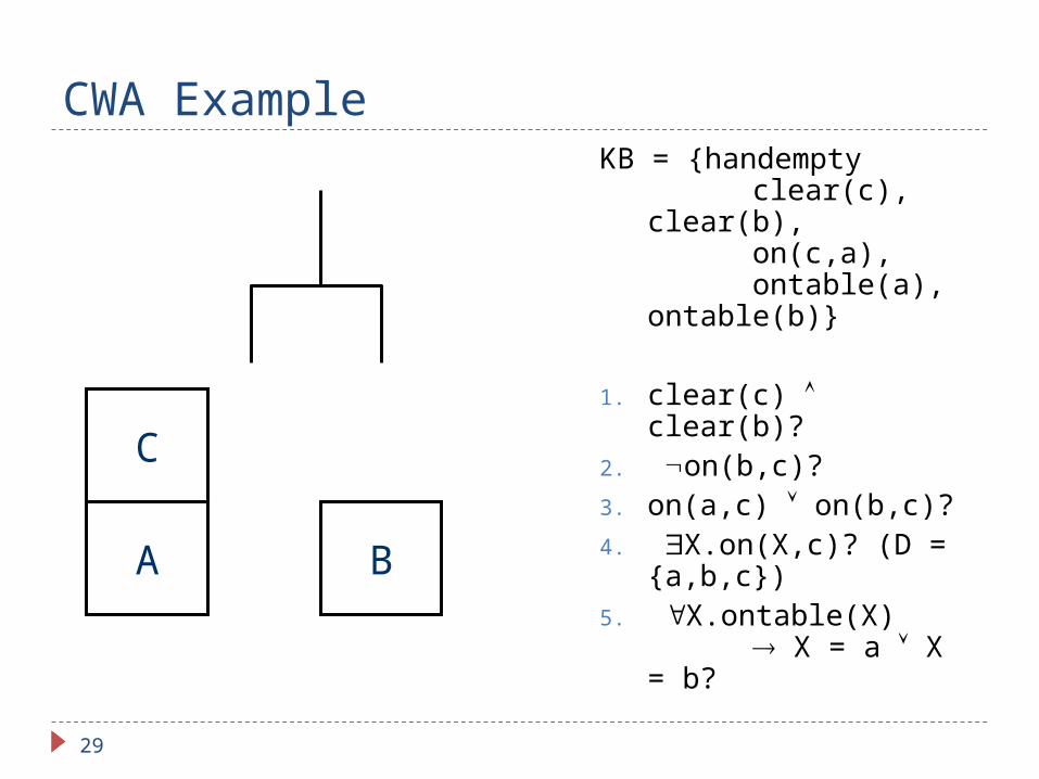
CWA ExampleKB = {handempty

clear(c), clear(b), on(c,a), ontable(a), ontable(b)}

1. clear(c) clear(b)?2. on(b,c)?3. on(a,c) on(b,c)?4. X.on(X,c)? (D =

{a,b,c})5. X.ontable(X)

X = a X = b?

29

C

A B

Querying a Closed World KB With the CWA, we can evaluate the truth or

falsity of arbitrarily complex first-order formulas.

This process is very similar to query evaluation in databases.

Just as databases are useful, so are CW KB’s.

30

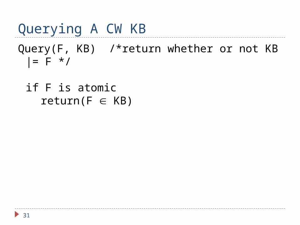
Querying A CW KBQuery(F, KB) /*return whether or not KB |= F */

if F is atomicreturn(F KB)

31

Querying A CW KBif F = F1 F2

return(Query(F1) && Query(F2))

if F = F1 F2

return(Query(F1) || Query(F2))

if F = F1

return(! Query(F1))

if F = F1 F2

return(!Query(F1) || Query(F2))

32

Querying A CW KBif F = X.F1

for each constant c KB

if (Query(F1{X=c}))return(true)

return(false).

if F = X.F1


if (!Query(F1{X=c}))return(false)

return(true).

33

Querying A CW KBGuarded quantification (for efficiency).

if F = X.F1


if (!Query(F1{X=c}))return(false)

return(true).

E.g., consider checking X. apple(x) → sweet(x)

we already know that the formula is true for all “non-apples”

34

Querying A CW KBGuarded quantification (for efficiency).

X:[p(X)] F1 X: p(X) → F1

for each constant c s.t. p(c)if (!Query(F1{X=c}))

return(false)return(true).

X:[p(X)]F1 X: p(X) F1

for each constant c s.t. p(c)if (Query(F1{X=c}))

return(true)return(false).

35

STRIPS representation. STRIPS (Stanford Research Institute Problem

Solver.) is a way of representing actions. Actions are modeled as ways of modifying the

world. since the world is represented as a CW-KB, a

STRIPS action represents a way of updating the CW-KB.

Now actions yield new KB’s, describing the new world—the world as it is once the action has been executed.

36

Sequences of Worlds In the situation calculus where in one logical

sentence we could refer to two different situations at the same time.

on(a,b,s0) on(a,b,s1)

In STRIPS, we would have two separate CW-KB’s. One representing the initial state, and another one representing the next state (much like search where each state was represented in a separate data structure).

37

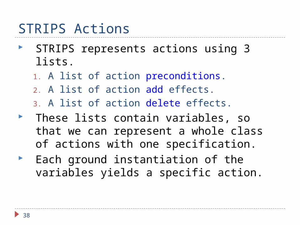
STRIPS Actions STRIPS represents actions using 3 lists.

1. A list of action preconditions.2. A list of action add effects.3. A list of action delete effects.

These lists contain variables, so that we can represent a whole class of actions with one specification.

Each ground instantiation of the variables yields a specific action.

38

STRIPS Actions: Examplepickup(X): Pre: {handempty, clear(X), ontable(X)}Adds: {holding(X)}Dels: {handempty, clear(X), ontable(X)}

“pickup(X)” is called a STRIPS operator.a particular instance e.g.“pickup(a)” is called an action.

39

Operation of a STRIPS action. For a particular STRIPS action (ground

instance) to be applicable to a state (a CW-KB) every fact in its precondition list must be true in

KB. This amounts to testing membership since we have

only atomic facts in the precondition list. If the action is applicable, the new state is

generated by removing all facts in Dels from KB, then adding all facts in Adds to KB.

40

Operation of a Strips Action: Example

41

KB = {handempty clear(c), clear(b), on(c,a), ontable(a), ontable(b)}

CA B

CA

Bpickup(b

)

KB = { holding(b),clear(c),

on(c,a), ontable(a)}

pre = {handmpty, clear(b), ontable(b)}

add = {holding(b)}

del = {handmpty, clear(b), ontable(b)}

STRIPS Blocks World Operators. pickup(X)

Pre: {clear(X), ontable(X), handempty}Add: {holding(X)}Del: {clear(X), ontable(X), handempty}

putdown(X)Pre: {holding(X)}Add: {clear(X), ontable(X), handempty}Del: {holding(X)}

42

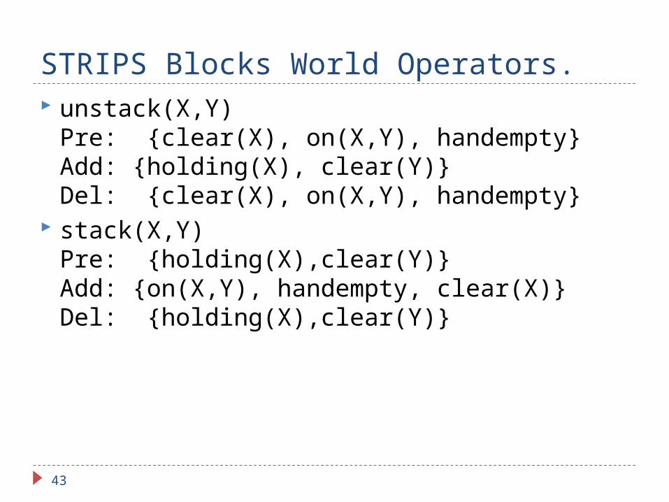
STRIPS Blocks World Operators. unstack(X,Y)

Pre: {clear(X), on(X,Y), handempty}Add: {holding(X), clear(Y)}Del: {clear(X), on(X,Y), handempty}

stack(X,Y)Pre: {holding(X),clear(Y)}Add: {on(X,Y), handempty, clear(X)}Del: {holding(X),clear(Y)}

43

STRIPS has no Conditional Effects putdown(X)

Pre: {holding(X)}Add: {clear(X), ontable(X), handempty}Del: {holding(X)}

stack(X,Y)Pre: {holding(X),clear(Y)}Add: {on(X,Y), handempty, clear(X)}Del: {holding(X),clear(Y)}

The table has infinite space, so it is always clear. If we “stack(X,Y)” if Y=Table we cannot delete clear(Table), but if Y is an ordinary block “c” we must delete clear(c).

44

Conditional Effects Since STRIPS has no conditional effects, we

must sometimes utilize extra actions: one for each type of condition.

We embed the condition in the precondition, and then alter the effects accordingly.

45

ADL Operators.ADL operators add a number of features to STRIPS.1. Their preconditions can be arbitrary formulas,

not just a conjunction of facts.2. They can have conditional and universal effects. 3. Open world assumption:

1. States can have negative literals2. The effect (P∧¬Q) means add P and ¬Q but delete ¬ P

and Q.

But they must still specify atomic changes to the knowledge base (add or delete ground atomic facts).

46

ADL Operators Examples.move(X,Y,Z)Pre: on(X,Y) clear(Z)Effs: ADD[on(X,Z)] DEL[on(X,Y)]

Z table DEL[clear(Z)] Y table ADD[clear(Y)]

47

ADL Operators, example

48

KB = { clear(c), clear(b), on(c,a), on(a,table), on(b,table)}

CA B

CA B

move(c,a,b)

KB = { on(c,b) clear(c), clear(a) on(a,table), on(b,table)}

move(c,a,b)Pre: on(c,a) clear(b)Effs: ADD[on(c,b)] DEL[on(c,a)]b table DEL[clear(b)]a table ADD[clear(a)]

ADL Operators Examples.clearTable()Pre: Effs: X. on(X,table) DEL[on(X,table)]

49

ADL Operators.1. Arbitrary formulas as preconditions.

in a CW-KB we can evaluate whether or not the preconditions hold for an arbitrary precondition.

2. They can have conditional and universal effects. Similarly we can evaluate the condition to see if

the effect should be applied, and find all bindings for which it should be applied.

Specify atomic changes to the knowledge base. CW-KB can be updated just as before.

50

Other Example Domains 8 Puzzle as a planning problem

A constant representing each position, P1,…,P9 A constant for each tile. B,T1, …, T8.

51

P1 P2 P3

P4 P5 P6

P7 P8 P9

8-Puzzle at(T,P) tile T is at position P.

adjacent(P1,P2) P1 is next to P2 (i.e., we can slide the blank from P1 to P2 in one move. adjacent(P5,P2), adjacent(P5,P8), …

52

1 2 5

7 8

6 4 3

at(T1,P1), at(T2,P2), at(T5,P3), …

8-Puzzleslide(T,X,Y)

Pre: {at(T,X), at(B,Y), adjacent(X,Y)} Add: {at(B,X), at(T,Y)} Del: {at(T,X), at(B,Y)}

53

1 2 5

7 8

6 4 3

at(T1,P1), at(T5,P3), at(T8,P5), at(B,P6), …,

slide(T8,P5,P6)

1 2 5

7 8

6 4 3

at(T1,P1), at(T5,P3), at(B,P5), at(T8,P6), …,

Elevator Control

54

Elevator Control Schindler Lifts.

Central panel to enter your elevator request. Your request is scheduled and an elevator is

assigned to you. You can’t travel with someone going to a secure

floor, emergency travel has priority, etc. Modeled as a planning problem and fielded in

one of Schindler’s high end elevators.

55

Solving Planning Problems Given a CW-KB representing the initial state, a

set of STRIPS or ADL (Action Description Language) operators, and a goal condition we want to achieve (specified either as a conjunction of facts, or as a formula)

The planning problem is determine a sequence of actions that when applied to the initial CW-KB yield an updated CW-KB which satisfies the goal.

56

Solving Planning ProblemsGraphPlan

GraphPlan is an approach to planning that is built on the idea of building a graph to represent the planning problem.

The performance is not at good as heuristic search (which we will discuss later), but GraphPlan does perform better than partial-order planning and it can be generalized to other types of planning, e.g., finding optimal plans, planning with sensing, etc.

57

Graphplan Operates in two phases.

Phase I. Guess a “concurrent” plan length k, then build a leveled graph with k alternating layers.

Phase II. Search this leveled graph for a plan. If no plan is found, return to phase I and build a bigger leveled graph with k+1 alternating layers. The final plan, if found, consists of a sequence of sets of actions

{a11,a2

1,…} → {a12, a2

2,…} → {a13, a2

3, …} → …

The plan is “concurrent” in the sense that at stage I, all actions in the i-th set can be executed in any order (or in parallel).

58

Graphplan The leveled graph alternates between levels

containing propositional nodes and levels containing action nodes.

Three types of edges: precondition-edges, add-edges, and delete-edges.

59

GraphPlan Level Graph

60

onTable(A)onTable(B)clear(A)clear(B)handempty

Initial state

Only the propositions true in the initial state.

All propositions added by actions in previous level

Possible actions

Only the actions whose preconditions are in the previous level.

Also have no-ops for capturing non-changes.

holding(A)holding(B)onTable(A)onTable(B)clear(A)clear(B)handempty

pickup(A)pickup(B)no-op(onTable(A))no-op(onTable(B))no-op(Clear(A))no-op(Clear(B))no-op(handempty)

Precondition

Delete

Add

GraphPlan Level Graph

61


Level S0 contains all facts true in the initial state.

Level A0 contains all actions whose preconditions are true in S0. Included in the set of actions are no-ops. One no-op for every ground atomic fact. The precondition of the no-op is its fact, its add effect is its fact.

…

Level Si contains all facts that are added by actions at level Ai-1

Level Ai contains all actions whose preconditions are true in Si



GraphPlan Mutexes.

62


In addition to the facts/actions. GraphPlan also computes and adds mutexes to the graph.

Mutexes are edges between two labels, indicating that these two labels cannot be true at the same time.

Mutexes are added as we construct each layer, and in fact alter the set of labels the eventually appear in a layer.



Mutexes A mutex between two actions a1 and a2 in the

same layer Ai, means that a1 and a2 cannot be executed simultaneously (in parallel) at the ith step of a concurrent plan.

A mutex between two facts F1 and F2 in the same state layer Si, means that F1 and F2 cannot be be simultaneously true after i stages of parallel action execution.

63

Mutexes It is not possible to compute all mutexes.

This is as hard as solving the planning problem, and we want to perform mutex computation as a precursor to solving a planning instance.

However, we can quickly compute a subset of the set of all mutexes. Although incomplete these mutexes are still very useful.

This is what GraphPlan does.

64

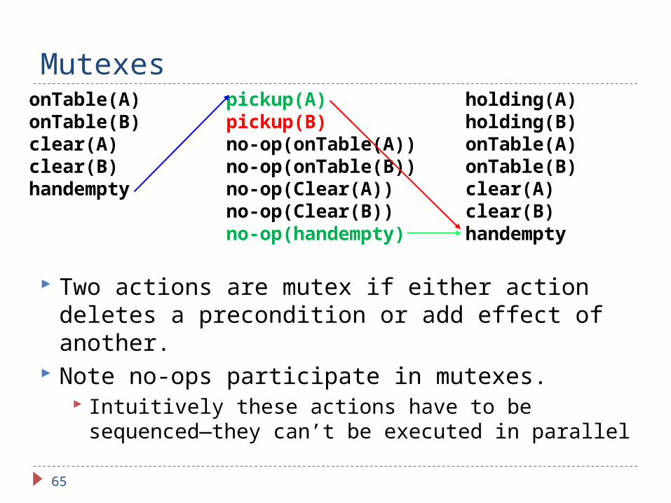
Mutexes

Two actions are mutex if either action deletes a precondition or add effect of another.

Note no-ops participate in mutexes. Intuitively these actions have to be sequenced—

they can’t be executed in parallel

65




Mutexes

Two propositions p and q are mutex if all actions adding p are mutex of all actions adding q.

Must look at all pairs of actions that add p and q. Intuitively, can’t achieve p and q together at this

stage because we can’t concurrently execute achieving actions for them at the previous stage.

66




Mutexes

Two actions are mutex if two of their preconditions are mutex.

Intuitively, we can’t execute these two actions concurrently at this stage because their preconditions can’t simultaneously hold at the previous stage.

67

putdown(A)putdown(B)no-op(onTable(A))no-op(onTable(B))no-op(Clear(A))no-op(Clear(B))no-op(handempty)


How Mutexes affect the level graph.1. Two actions are mutex if either action deletes a

precondition or add effect of another2. Two propositions p and q are mutex if all actions adding p

are mutex of all actions adding q3. Two actions are mutex if two of their preconditions are

mutex We compute mutexes as we add levels.

S0 is set of facts true in initial state. (Contains no mutexes).

A0 is set of actions whose preconditions are true in S0. Mark as mutex any action pair where one deletes a

precondition or add effect of the other. S1 is set of facts added by actions at level A0.

Mark as mutex any pair of facts p and q if all actions adding p are mutex with all actions adding q.

A1 is set of actions whose preconditions are not mutex at S1. Mark as mutex any action pair with preconditions that

are mutex in S1, or where one deleted a precondition or add effect of the other.

68

How Mutexes affect the level graph.1. Two actions are mutex if either action deletes a

precondition or add effect of another2. Two propositions p and q are mutex if all actions adding

p are mutex of all actions adding q3. Two actions are mutex if two of their preconditions are

mutex

… Si is set of facts added by actions in level Ai-1

Mark as mutex all facts satisfying 2 (where we look at the action mutexes of Ai-1 is set of facts true in initial state. (Contains no mutexes).

Ai is set of actions whose preconditions are true and non-mutex at Si. Mark as mutex any action pair satisfying 1 or 2.

69

How Mutexes affect the level graph. Hence, mutexes will prune actions and facts

from levels of the graph. They also record useful information about

impossible combinations.

70

Example

71

on(a,b), ontable(c),ontable(b),clear(a),clear(c),handempty

unstack(a,b)

pickup(c)

on(a,b),on(b,c),ontable(c),ontable(d),clear(a),clear(c),handempty,holding(a),clear(b),holding(c)

preconditionadd effectdel effect

pickup deletes handempty, one of unstack(a,b)’s preconditions.

NoOp-on(a,b)

unstack(a,b) deletes the add effect of NoOp-on(a,b), so these actions are mutex as well

Example

72


unstack(a,b) is the only action that adds clear(b), and this is mutex with pickup(c), which is the only way of adding holding(c).


unstack(a,b)

pickup(c)


NoOp-on(a,b)

Example

73


These two are mutex for the same reason.on(a,b),

ontable(c),ontable(b),clear(a),clear(c),handempty

unstack(a,b)

pickup(c)


NoOp-on(a,b)

Example

74


unstack(a,b) is also mutex with the NoOp-on(a,b).So these two facts are mutex (NoOp is the only way on(a,b) can be created).


unstack(a,b)

pickup(c)


NoOp-on(a,b)

Phase II. Searching the Graphplan

Build the graph to level k, such that every member of the goal is present at level k, and no two are mutex. Why?

75

on(A,B)on(B,C)onTable(c)onTable(B)clear(A)clear(B)handempty

K

Searching the Graphplan

Find a non-mutex collection of actions that add all of the facts in the goal.

76


stack(A,B)stack(B,C)no-op(on(B,C))...

K

Searching the Graphplan

The preconditions of these actions at level K-1 become the new goal at level K-1.

Recursively try to solve this new goal. If this fails, backtrack and try a different set of actions for solving the goal at level k.

77


K

stack(A,B)stack(B,C)no-op(on(B,C))...

holding(A)clear(B)on(B,C)

K-1

Phase II-Search Solve(G,K)

forall sets of actions A={ai} such thatno pair (ai, aj) A is mutexthe actions in A suffice to add all facts in G

Let P = union of preconditions of actions in A If Solve(P,K-1)

Report PLAN FOUND At end of forall. Exhausted all possible action sets

AReport NOPLAN

This is a depth first search.

78

Graph Plan Algorithm Phase I. build leveled graph. Phase II. Search leveled graph.

Phase I: While last state level does not contain all goal facts with no pair being mutex

add new state/action level to graph if last state/Action level = previous state/action level

(including all MUTEXES) graph has leveled off) report NO PLAN.

Phase II: Starting at last state level search backwards in graph for plan. Try all ways of moving goal back to initial state.

If successful report PLAN FOUND. Else goto Phase I.

79

Dinner Date Example Initial State

{dirty, cleanHands, quiet} Goal

{dinner, present, clean} Actions

Cook: Pre: {cleanHands}Add: {dinner}

Wrap: Pre: {quiet}Add: {present}

Tidy: Pre: {}Add: {clean}Del: {cleanHands, dirty}

Vac: Pre: {}Add: {clean}Del: {quite, dirty}

80

Dinner Date Example

81

Solving Planning ProblemsPlanning As Search This can be treated as a search problem.

The initial CW-KB is the initial state. The actions are operators mapping a state (a CW-

KB) to a new state (an updated CW-KB). The goal is satisfied by any state (CW-KB) that

satisfies the goal.

82

Example.

83

CA B

move(b,c) CA

B

move(c,b)C

A B

move(c,table) CA B

move(a,b)BA C

Problems Search tree is generally quite large

randomly reconfiguring 9 blocks takes thousands of CPU seconds.

The representation suggests some structure. Each action only affects a small set of facts, actions depend on each other via their preconditions.

Planning algorithms are designed to take advantage of the special nature of the representation to compute useful heursitics.

84

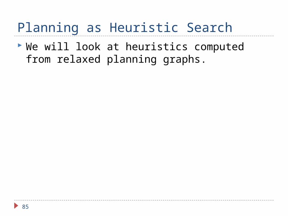
Planning as Heuristic Search We will look at heuristics computed from

relaxed planning graphs.

85

Relaxed Plans. The idea is to consider what happens if we

ignore the delete lists of actions. This is yields a “relaxed problem” that can

produce a useful heuristic estimate.

86

Finding Relaxed Plans In the relaxed problem actions add new facts, but

never delete facts. Given the relaxed planning problem we use GraphPlan

to build a plan for solving the relaxed problem. We then take the number of steps in the GraphPlan

plan as a heuristic estimate of the distance from the current state to the goal. This is the method used by the Fast Forward System you

are employing in your assignment.

It turns out that this heuristic is not admissible. It is possible to compute admissible heuristics, but in general they don’t perform as well: they force the planner to find optimal plans.

87

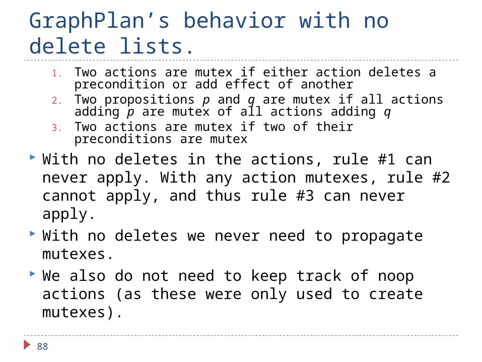
GraphPlan’s behavior with no delete lists.

1. Two actions are mutex if either action deletes a precondition or add effect of another

2. Two propositions p and q are mutex if all actions adding p are mutex of all actions adding q

3. Two actions are mutex if two of their preconditions are mutex

With no deletes in the actions, rule #1 can never apply. With any action mutexes, rule #2 cannot apply, and thus rule #3 can never apply.

With no deletes we never need to propagate mutexes.

We also do not need to keep track of noop actions (as these were only used to create mutexes).

88

GraphPlan’s behavior with no delete lists. Going through the graph plan procedure we see than on

relaxed plans the process is simplified to the following

1. We start with the initial state S0.

2. We alternate between state and action layers.

3. We find all actions whose preconditions are contained in S0. These actions comprise the first action layer A0.

4. The next state layer consists of all of S0 as well as the adds of all of the actions in A0.

5. In general Ai is the set of actions whose preconditions are contained in

Si.

Si+1 is Si union the add lists of all of the actions in Ai.

89

Example

90

a

b

c d

on(a,b),on(b,c),ontable(c),ontable(d),clear(a),clear(d),handempty

unstack(a,b)pickup(d)

ab

c d

S0 A0

on(a,b),on(b,c),ontable(c),ontable(d),clear(a),handempty,clear(d),holding(a),clear(b),holding(d)

ad

this is not a state!

S1

Example

91

on(a,b),on(b,c),ontable(c),ontable(d),clear(a),clear(d),handempty,holding(a),clear(b),holding(d)

S1

putdown(a),putdown(d),stack(a,b),stack(a,a),stack(d,b),stack(d,a),pickup(d),…unstack(b,c)…

A1

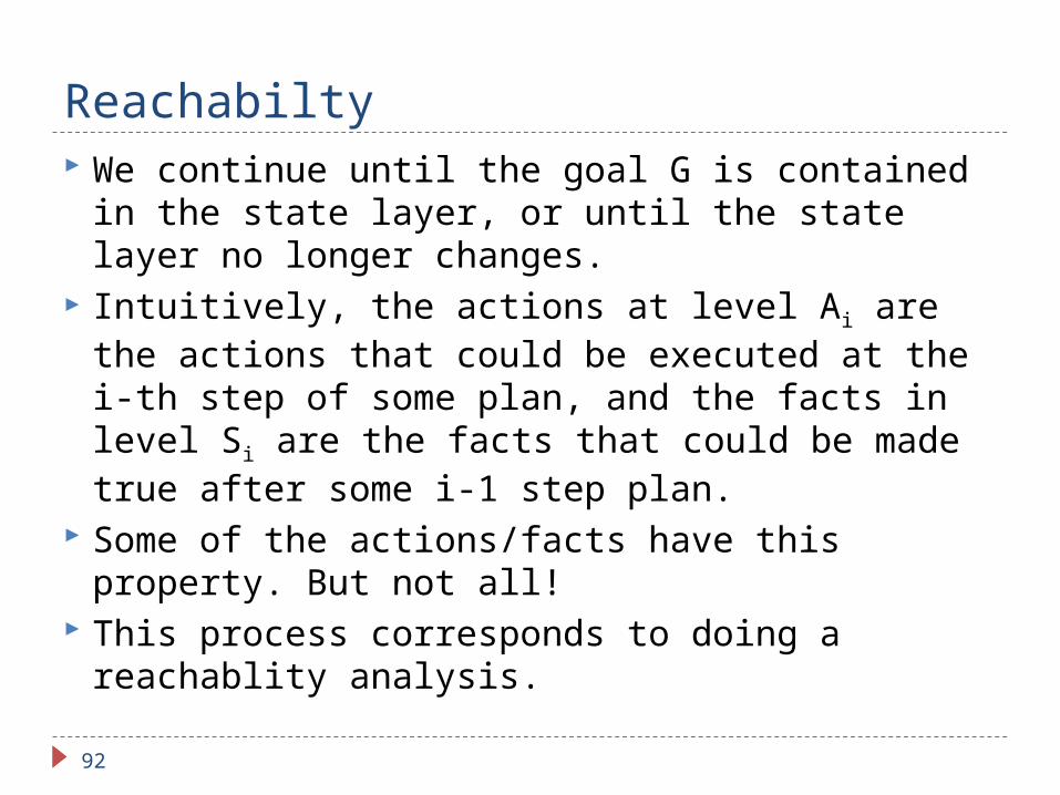
Reachabilty We continue until the goal G is contained in the

state layer, or until the state layer no longer changes.

Intuitively, the actions at level Ai are the actions that could be executed at the i-th step of some plan, and the facts in level Si are the facts that could be made true after some i-1 step plan.

Some of the actions/facts have this property. But not all!

This process corresponds to doing a reachablity analysis.

92

Reachability

93

a

b c

on(a,b),on(b,c),ontable(c),ontable(b),clear(a),clear(c),handempty

unstack(a,b)pickup(c)

S0 A0

on(a,b),on(b,c),ontable(c),ontable(b),clear(a),clear(c),handempty,holding(a),clear(b),holding(c)

S1

stack(c,b)…

A1

…on(c,b),…

but stack(c,b) cannot be executed after one step

and on(c,b) needs 4 actions

Heuristics from Reachability AnalysisGrow the levels until the goal is contained in the

final state level S[K]. If the state level stops changing and the goal is

not present. The goal is unachievable. (The goal is a set of positive facts, and in STRIPS all preconditions are positive facts).

We search the graph to extract a plan (Phase II of the graph plan process).

94

Phase II of Graphplan Solve(G,K)

forall sets of actions A={ai} such thatno pair (ai, aj) A is mutexthe actions in A suffice to add all facts in G

Let P = union of preconditions of actions in A If Solve(P,K-1)

Report PLAN FOUND At end of forall. Exhausted all possible action sets A

Report NOPLAN

Relaxed plan graph contains no mutexes. So the recursive call to Solve(P,K-1) will never fail.

Additionally since we don’t have no-ops in the graph, we need to change the test “suffice to add all facts in G” (some facts were previously created at earlier levels and “added” by no-ops. Without the no-ops we have to “delay” these facts.

95

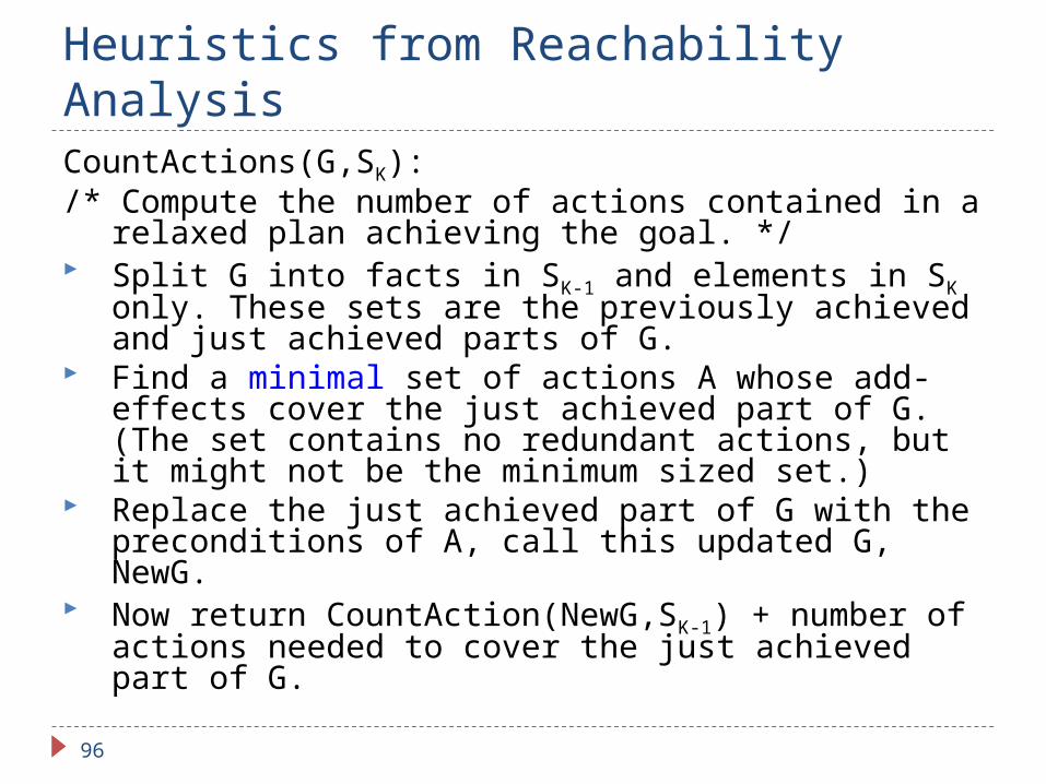
Heuristics from Reachability AnalysisCountActions(G,SK):/* Compute the number of actions contained in a

relaxed plan achieving the goal. */ Split G into facts in SK-1 and elements in SK only.

These sets are the previously achieved and just achieved parts of G.

Find a minimal set of actions A whose add-effects cover the just achieved part of G. (The set contains no redundant actions, but it might not be the minimum sized set.)

Replace the just achieved part of G with the preconditions of A, call this updated G, NewG.

Now return CountAction(NewG,SK-1) + number of actions needed to cover the just achieved part of G.

96

Example legend: [pre]act[add]S0 = {f1, f2, f3}

A0 = {[f1]a1[f4], [f2]a2[f5]}

S1 = {f1,f2,f3,f4,f5}

A1 = {[f2,f4,f5]a3[f6]}

S2 ={f1,f2,f3,f4,f5,f6}

G = {f6,f5, f1}

We split G into GP and GN:

97

CountActs(G,S2)

GP ={f5, f1} //already in

S1

GN = {f6} //New in S2

A = {a3} //adds all in

GN

//the new goal: GP Pre(A)

G1 = {f5,f1,f2,f4}

Return 1 + CountActs(G1,S1)

ExampleNow, we are at level S1S0 = {f1, f2, f3}

A0 = {[f1]a1[f4], [f2]a2[f5]}

S1 = {f1,f2,f3,f4,f5}

A1 = {[f2,f4,f5]a3[f6]}

S2 ={f1,f2,f3,f4,f5,f6}

G1 = {f5,f1,f2,f4}

We split G1 into GP and GN:

98

CountActs(G1,S1)

GP ={f1,f2} //already in

S0

GN = {f4,f5} //New in S1

A = {a1,a2} //adds all in

GN

//the new goal: GP Pre(A)

G2 = {f1,f2}

Return 2 + CountActs(G2,S0)

= 2 + 0

So, in total CountActs(G,S2)=1+2=3

Using the Heuristic1. To use CountActions as a heuristic, we build

a layered structure from a state S that reaches the goal.

2. Then we CountActions to see how many actions are required in a relaxed plan.

3. We use this count as our heuristic estimate of the distance of S to the goal.

4. This heuristic tends to work better as a best-first search, i.e., when the cost of getting to the current state is ignored.

99

Admissibility An optimal length plan in the relaxed problem

(actions have no deletes) will be a lower bound on the optimal length of a plan in the real problem.

However, CountActions does NOT compute the length of the optimal relaxed plan.

The choice of which action set to use to achieve GP (“just achieved part of G”) is not necessarily optimal.

In fact it is NP-Hard to compute the optimal length plan even in the relaxed plan space.

So CountActions will not be admissible.

100

Empirically However, empirically refinements of

CountActions performs very well on a number of sample planning domains.

101

1 Planning (under complete Knowledge) Intro to Artificial Intelligence.

Documents

Transcript of 1 Planning (under complete Knowledge) Intro to Artificial Intelligence.