1

On the Relationship between theUnderwater Acoustic and Optical Channels

Roee Diamant, Filippo Campagnaro, Michele De Filippo De Grazia,

Paolo Casari, Senior Member, IEEE, Alberto Testolin,

Violeta Sanjuan Calzado, Michele Zorzi, Fellow, IEEE

Abstract

Wireless transmissions in water are mostly carried out via long-range (but low-rate) underwater acoustic

communications, or short-range (but high-rate) underwater optical communications. In this paper we are

interested in finding whether a statistical relationship exists between underwater acoustics and optics.

Besides the theoretical interest of such relationship, predicting the quality of the optical link through

acoustics is also relevant in the context of a multimodal system with both acoustics and optics. Our study

is based on a large dataset acquired during the NATO ALOMEX’2015 expedition. During this experiment,

we simultaneously measured several characteristics of the acoustic and optical links at multiple locations,

reflecting a diversity of sea environments. Our results, show a strong correlation between the properties of

the acoustic link and the reliability of optical communications. This correlation makes it possible to predict

the state of the underwater optical link at a certain depth and range. Due to the complexity of the acoustic

and optical channels, we could not find the source of this correlation. This work is therefore aimed to

stimulate a theoretical study of the mutual properties of underwater acoustic and optical communication

links. For reproducibility, we share the processed data from the experiment.

Index Terms

Underwater acoustic communications; Underwater optical communications; Multimodal systems; Sup-

port vector machine; Machine learning; Classification; Prediction; Sea Experiment

R. Diamant (e-mail: roeed@univ.haifa.ac.il) is with the Department of Marine Technology, University of Haifa, Israel.

F. Campagnaro and M. Zorzi are with the Department of Information Engineering, University of Padova, Italy. M. de Filippo

de Grazia and A. Testolin are with the Department of General Psychology, University of Padova, Italy. P. Casari is with the

IMDEA Networks Institute, Madrid, Spain.

2

I. INTRODUCTION

In the last decade, ocean exploration has increased considerably through underwater surveys.

The purposes of these surveys include bathymetry mapping and natural resource prospection,

maintenance (environmental monitoring and structural inspection of underwater facilities such as

drilling devices and pipelines), and securing marine infrastructures against intruders. The ability

to wirelessly exchange information among submerged devices is a key enabling technology to

perform these tasks. Currently, the two top technologies for underwater wireless transmission are

underwater acoustic communications (AC) and underwater optical communications (OC). AC is

characterized by long-range (in the order of tens of km) but low-data-rate transmissions (up to a

few kbps), and is considered highly unreliable due to the limited bandwidth, long delay spread,

short channel coherence time, and dispersiveness that characterize the acoustic channel [1]. OC

features high data rates (in the order of Mbps), but is only suitable over much shorter transmission

ranges (in the order of tens of meters) [2].

AC and OC are driven by different physics. The former involves the propagation of a pressure

wave and is modeled, e.g., via the so-called normal modes [3], [4] or empirical equations [5],

whereas the latter is performed via electromagnetic waves whose propagation is driven by the

radiative transfer equations [6]. The sources of noise in the underwater acoustic channel are also

much different than those that affect the optical channel [7]. While shipping noise and sea waves

are the main sources of noise in AC [3], the irradiance and scattering of sunlight in the water are

the main factors that affect OC. Although these models are seemingly unrelated, it is of theoretical

interest to show if there exists a combination of underwater acoustic properties that can be exploited

to predict the state of the underwater optical link. Specifically, we are mainly interested in finding

a relationship between the measured physical characteristics of the underwater acoustic link and

the following two estimates:

1) a binary (good/bad) state of OC at a certain range and depth;

2) the signal-to-noise ratio (SNR) of OC at a given range and depth.

The first item is a classification problem, whereas the second item implies a regression and

3

prediction problem.

While finding a relation between the AC and OC is of theoretical interest per se, such relation

also has several practical applications. First, it would assist in predicting the characteristics of OC

through AC. This will significantly reduce the cost and complexity of obtaining OC measurements,

which otherwise require specialized equipment [8], [9]. Second, by predicting the quality of OC

through AC, a mobile node which holds both communication systems can be guided to a location

where both technologies can be efficiently used. This application is specifically important for

multimodal underwater communication systems, where both OC and AC are utilized [10]. For

example, by predicting the properties of OC, an autonomous underwater vehicle (AUV) equipped

with both AC and OC [11] can be directed to the maximal1 range and depth still allowing

reliable communication with the hub. Third, exploiting a relationship between OC and AC would

enable more effective switching mechanisms than the current range-based triggering of OC, which

only reflects the communication system specifications, and not the actual characteristics of the

communication channel [7].

In this work, we study the relationship between AC and OC from a statistical point of view.

Specifically, we investigate whether, for a given range and depth, the properties of an underwater

AC link can be used for classifying OC link quality and for predicting the SNR over OC links.

We limit our application to environments like the open sea, where it can be assumed that the

properties of the optical link change slowly in time and space. While we were unable to find a

theoretical/mathematical explanation for the relation between the AC and the OC, we present sta-

tistical evidence that this relation exists. It is our hope to stimulate further theoretical investigations

in this direction.

Our study is based on a large dataset of acoustic and optical link properties simultaneously

measured over a prolonged time span and over different frequency bands. Our dataset was obtained

during the ALOMEX 2015 experiment led by the NATO STO CMRE, La Spezia, Italy. Using this

1For safety reasons, the AUV should avoid a close contact with the receiver.

4

dataset, we trained different learning models based on support vector machines (SVMs) [12], with

the goal of classifying the corresponding quality of the optical link and predicting the optical SNR

at various distances and depths. The learning system was designed and tuned to maximize the

classification and prediction accuracy, while at the same time avoiding overfitting.

Our results show a strong correlation between the properties of the underwater acoustic link

and the overall quality of OC. Moreover, using the acoustic properties as predictors, we show that

the SNR of the OC link can be estimated with a sufficient degree of accuracy to enable ambient

intelligence in underwater communication systems. This surprising result not only provides a tool

for combining AC and OC, but also justifies further theoretical studies targeting the relationship

between the underwater acoustic and optical links. Our contribution is therefore three-fold and

includes:

1) an extensive quantitative study of the relationship between AC and OC;

2) a comparison between such relation at different acoustic frequency bands;

3) a dataset freely shared with the community for further investigation of the link between

underwater acoustics and optics, and for the design of multimodal AC/OC systems.

The remainder of this paper is organized as follows. An overview of AC, OC, and multimodal

systems is given in Section II, which also provides the basics of the machine learning techniques

employed for data analysis. A detailed description of the acquired dataset is given in Section III.

The methods and results of the quantitative study are described in Section IV. Finally, we draw

our conclusions in Section V.

II. PRELIMINARIES

A. Basics of AC

Substantial differences exist between long-range deep water AC and short-range shallow water

AC. Since multimodal systems are used for relatively short ranges of a few km, we focus on

the latter. The shallow water underwater channel is a time-varying frequency-selective channel,

characterized by a long delay spread [13] and a coherence time on the order of tens of ms [14].

5

Given the low transmission rate (common systems achieve a few kbps [15]), such long channel

and short coherence time pose a challenge for channel equalization [16]. Since the sea surface is

continuously in motion, individual channel taps are affected by a Doppler shift that, depending

on the carrier frequency, may vary up to tens of Hz [17]. Due to the low sound speed (roughly

1500 m/s), this Doppler shift affects the duration of the received signal and, therefore, cannot be

fully compensated by a phase-locked loop. Instead, interpolation is generally required [18]. The

key parameters to predict the integrity of AC are the number of channel taps, their power and

propagation delay, and the variation of these characteristics over time.

Besides the channel impulse response and the power attenuation, AC is also highly affected by

the channel ambient noise. The ambient noise is usually modeled as an isotropic colored Gaussian

noise whose power spectral density reduces by 10 dB per octave [19]. However, the acoustic

ambient noise may also include location-dependent, non-isotropic noise which may affect the

performance of AC. The sources of such noise are acoustic transmissions from nearby ships, short

noise transients from marine fauna such as snapping shrimps, and wideband noise from breaking

waves, especially when the receiver is close to the water surface [20]. Thus, besides the noise level

itself, the time-varying characteristics of the noise also affect the performance of AC.

The SNR (in dB) of a transmission performed at a frequency fa over a distance d between the

transmitter and the receiver is found as [3]

SNR(d, fa) = 10 log10

(Pa

N(fa) δfa

)− A(d, fa) , (1)

where Pa is the source level (usually expressed in dB relative to 1 µPa @ 1 m from the source),

N(fa) is the noise level, A(d, fa) is the power attenuation in dB, and δfa is a narrow band around

fa where we can assume A(d, f) = A(d, fa) and N(f) = N(fa).

B. Basics of OC

Light traveling in the water interacts with the particulates and dissolved materials within the

water as well as the water molecules themselves. These interactions produce light attenuation

(modeled via an attenuation rate per unit length traveled by the wave, and termed c) that will

6

determine the underwater light field, or radiance, denoted as L, and defined as the measure of light

energy leaving an extended source in a particular direction.

The parameters L and c are related through the radiative transfer equation (RTE), which relates

the apparent and inherent optical properties of the medium [6]. The light attenuation rate c, the

optical absorption rate a, and the loss rate due to scattering processes b are related as

c = a+ b . (2)

If the inherent optical properties of the medium depend only on depth, inelastic processes are

ignored, and there are no internal sources, the time-dependent RTE is described as [21]

cos θdL (z, λ, θ, φ)

dz= −c(z, λ)L(z, λ, θ, φ) +

∫4π

β (z, λ, θ′, φ′ → θ, φ)L (z, λ, θ′, φ′) dΩ′ , (3)

where β( · ) is called the volume scattering function and describes how the medium scatters light

per unit length and solid angle. The polar angle θ and the azimuthal angle φ of a spherical

coordinate system specify the scattered light direction, whereas the coordinates (θ′, φ′) inside the

integral convey the direction of the incident light. The integration limit denotes that the integral is

computed over the unit sphere surface, and we recall that dΩ′ = sin θ′ dθ′ dφ′. At a given depth and

wavelength, L is usually referred to as the radiance distribution. The first term on the right hand

side of (3) represents the loss of radiance in the direction (θ, φ) due to scattering and absorption,

while the second term provides the gain in radiance from all other directions (θ′, φ′) into the

direction (θ, φ). Analytical solutions of the RTE (3) are possible only if scattering is negligible.

Otherwise, as in the present work, (3) must be solved numerically. The most complete and accurate

method to do so is the successive-orders-of-scattering solution used in radiative transfer modeling

software such as Hydrolight [21].

Because radiance is difficult to measure, most light field measurements involve integrals of the

radiance distribution. For this study, we are interested in scalar irradiance, E0, i.e., the irradiance

measured over all directions, obtained by integrating radiance over the whole sphere as

E0(z, λ) =

∫4π

L(z, λ, θ, φ) dΩ . (4)

7

In the case of light transmission for underwater optical communications, this will be affected by

the ambient light, considered as noise. The ambient light noise power NA is obtained as

NA = (S · E0 · Ar)2 , (5)

where S is the sensitivity of the receiver and Ar is the receiver area.

In this work, we aim to prove a connection between the underwater acoustic channel and the

optical channel to predict the SNR of an optical communication system. While the literature

includes optical communication systems with range of hundreds of meters [22], these works use

a highly-directive laser source that requires perfect alignment between the transmitter and the

receiver, and assume very clear water (c = 0.063 1/m). Instead, we consider a LED-based optical

communication system whose semiaperture angle is three orders of magnitude larger than the

lasers, and thus imposes fewer limitations on system alignment. The considered system includes a

LED transmitter [23], and a Si PIN Hamamatsu photodiode [2] receiver. The achievable range is

between 2 and 50 m, depending on the water turbidity and the surrounding light noise. However,

we note that in this work we measured general underwater optical channel parameters. Thus, we

do not limit our conclusions to a certain type of optical system, and our conclusions regarding the

observed correlation between the underwater acoustic channel and the optical channel also apply

to e.g., laser-based underwater optical systems.

C. Intuitive Explanation for a Correlation between AC and OC

This paper focuses on presenting evidence about a correlation between AC and OC that allows

the classification of OC and the prediction of its SNR based on AC data. In the absence of a well

established theory for the relation between the two channels, in this section we give our intuitive

explanation for this correlation. Our main claim is that the quality of OC is mostly affected by the

turbidity of the water, and that this turbidity is generated by channel parameters that also affect

AC.

We start with the connection between acoustic noise and OC. The acoustic noise at shallow

water is dominated by the acoustic noise generated by the surface waves. Close to the surface,

8

these waves generate water bubbles and are a main contributor to the optical turbidity. Hence, the

noise level and the acoustical SNR are expected to have some relation with OC. Similarly, the

quality (or integrity) of AC that is affected by the acoustic noise is expected to have some link to

OC as well.

The optical turbidity is also very much affected by the number of scatterers in the water column,

for example plankton and floating sediments. These scatterers often also serve as acoustic volume

reflectors, which affect the structure of the underwater acoustic impulse response. Hence, we expect

that parameters like the channel’s length, the delay spread, and the number of taps, will have some

connection with the optical turbidity and therefore with the quality of OC. We also see a relation

between the number of scatterers in the water, which affects both the AC and the OC. Specifically,

the volume scatterers affect the optical propagation in water as well as the RMS of the AC’s

channel taps. Moreover, the number of scatterers in the channel is proportional to the acoustic

power absorption, and thus affects the received signal level of the AC.

Last, we note that the time dependency of AC is mostly affected by the motion in the channel.

In turn, this motion creates circulation in the water, that highly affects the water’s turbidity. Hence,

we expect to find a connection between the OC and measures like the channel coherence time and

the noise level coherence time that reflect the time-dependency of the channel.

D. Overview of Multimodal Systems

Multimodal systems combine AC with optical [2], [11] or radiofrequency [24], [25] communica-

tions, as well as AC systems working in different bands [26], [27]. Among these, OC seems to be

the most mature alternative to AC. In [28], a proof-of-concept for Orthogonal frequency-division

multiplexing (OFDM) based OC is described, and in [11] the capabilities of OC are demonstrated

for transmission of video over ranges of a few meters. Multimodal systems combining AC and OC

mostly involve a separate control over these two technologies. In [29], the sink-to-node downlink

is based on AC, and the uplink is serviced through OC. A similar concept is suggested in [30],

[31] where AC is used to request AUVs to approach and collect data through OC. On the contrary,

9

in [32], OC is employed for positioning of a swarm of AUVs, and AC is used for data exchange

between the AUVs.

A few works suggested a mechanism to switch between AC and OC so that data exchange

could be efficiently managed based on the current communication capabilities. This includes a

switching strategy based on the received power for each link [7], or based on the estimated distance

between the transmitter and the receiver [33]. MURAO is the first multimodal opto-acoustic routing

protocol [34]. It uses acoustic communications to help manage routing in a clustered multihop

optical network. The longer range acoustics connects cluster heads, thereby allowing sharing of

cluster information for inter-cluster communications.

E. Overview of the Machine Learning Approaches used for Data Analysis

In this paper, we focus on a particular class of supervised learning methods that can be formally

characterized using the statistical learning theory framework [35]. Statistical learning approaches

aim to infer the function that maps input data to output data, such that the learned function can

be used to predict the output from future input. In order to guarantee that the learned model

generalizes well to unseen data, statistical learning algorithms try to limit the complexity of the

resulting model to prevent overfitting. In particular, we use an efficient class of learning algorithms

called SVM [12]. An SVM tries to achieve the best separation between patterns belonging to

different classes by finding the maximum-separation hyperplane that has the largest distance to the

nearest training data point of any class. In general, the larger the distance margin, the lower the

generalization error of the classifier and the risk of overfitting the data. As a result, this learning

framework is particularly indicated when the available data is limited. A similar framework can be

applied in the case of real-valued outputs (regression tasks) using a variant called Support Vector

Regression (SVR) [36]. While our database is quite broad in terms of surveyed area, it is limited

in terms of number of measurements. For this reason, we have chosen SVM and SVR for the tasks

of classification and regression, respectively.

We consider both linear and non-linear SVMs. In linear SVM, we assume that the patterns

10

are linearly separable, and find two parallel hyperplanes whose distance is as large as possible to

separate the two classes of data. The equation of a linear SVM is expressed in the form

f(x) = 〈~w, ~x〉+ b , (6)

where 〈 , 〉 denotes the inner product in Rn, and the vector w and scalar b are used to define the

position of the maximum-margin separating hyperplane. Geometrically, the distance between the

two external hyperplanes is 2/‖~w‖, so in order to maximize their distance we want to minimize

‖~w‖. As we also have to prevent data points from falling into the margin, we add the following

constraints ∀ i: ~w · ~xi − b ≥ 1 if yi = 1

~w · ~xi − b ≤ −1, if yi = −1

. (7)

These constraints state that each data point must lie on the correct side of the margin. By introducing

Lagrange multipliers αi, the SVM training procedure amounts to solving a convex quadratic

problem. The solution is a unique globally optimum result, for which

~w =N∑i=1

αiyi~xi (8)

The terms ~xi are called support vectors. Once an SVM has been trained, the decision function can

simply be written as

f(~x) = sign

( N∑i=1

αiyi(〈~x, ~xi〉) + b

). (9)

The non-linear SVM uses the so-called kernel trick, implicitly mapping the inputs into higher-

dimensional feature spaces. The resulting algorithm is formally similar to the linear SVM, except

that every dot product is replaced by a non-linear kernel function K(~x, ~xi). This allows the

algorithm to fit the maximum-margin hyperplane in a transformed feature space. In this work

we use the popular Gaussian Radial Basis Function (RBF) kernel:

K(~x, ~xi) = exp(− |~x− ~xi|2/(2σ2)

). (10)

III. DESCRIPTION OF THE ACQUIRED DATASET

11

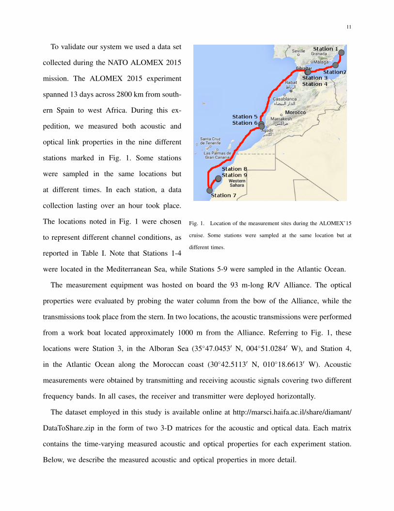
Fig. 1. Location of the measurement sites during the ALOMEX’15

cruise. Some stations were sampled at the same location but at

different times.

To validate our system we used a data set

collected during the NATO ALOMEX 2015

mission. The ALOMEX 2015 experiment

spanned 13 days across 2800 km from south-

ern Spain to west Africa. During this ex-

pedition, we measured both acoustic and

optical link properties in the nine different

stations marked in Fig. 1. Some stations

were sampled in the same locations but

at different times. In each station, a data

collection lasting over an hour took place.

The locations noted in Fig. 1 were chosen

to represent different channel conditions, as

reported in Table I. Note that Stations 1-4

were located in the Mediterranean Sea, while Stations 5-9 were sampled in the Atlantic Ocean.

The measurement equipment was hosted on board the 93 m-long R/V Alliance. The optical

properties were evaluated by probing the water column from the bow of the Alliance, while the

transmissions took place from the stern. In two locations, the acoustic transmissions were performed

from a work boat located approximately 1000 m from the Alliance. Referring to Fig. 1, these

locations were Station 3, in the Alboran Sea (3547.0453′ N, 00451.0284′ W), and Station 4,

in the Atlantic Ocean along the Moroccan coast (3042.5113′ N, 01018.6613′ W). Acoustic

measurements were obtained by transmitting and receiving acoustic signals covering two different

frequency bands. In all cases, the receiver and transmitter were deployed horizontally.

The dataset employed in this study is available online at http://marsci.haifa.ac.il/share/diamant/

DataToShare.zip in the form of two 3-D matrices for the acoustic and optical data. Each matrix

contains the time-varying measured acoustic and optical properties for each experiment station.

Below, we describe the measured acoustic and optical properties in more detail.

12

TABLE IEXPERIMENTAL MEASUREMENT STATIONS

# Location Date Time Temp. Depth Range Notes

13735.3729’N,0058.7448’W

Nov 1 13:40 18C 20 m 21 m Cartagena Harbor, instruments calibration

23625.0708’N,0140.0358’W

Nov 2 14:00 21C 128 m 52 m Rough sea, average wave height of 1 m

33545.4758’N,0455.6935’W

Nov 4 12:30 19C 129 m 57 m Calm sea

43547.0453’N,0451.0284’W

Nov 4 16:30 20.5C 119 m 1.3 km Calm sea, working boat

53042.5113’N,1018.6613’W

Nov 6 09:00 20.5C 127 m1 km,583 m

Calm ocean, working boat

63028.5720’N,1016.5030’W

Nov 6 15:30 20.5C 126 m 59 m Calm ocean

72351.1912’N,1619.4189’W

Nov 9 15:30 19.5C 40 m 45 mShallow/warm/turbid waters (Saharasandstorm)

82504.0009’N,1520.4917’W

Nov 10 09:30 22C 44 m 51 m Calm ocean with clear waters

92513.1351’N,1530.1324’W

Nov 10 13:45 22C 77 m 53 m Calm ocean with clear waters

A. Acoustic Properties

In the absence of a theory connecting underwater acoustics and underwater optics, to statistically

explore the relation between AC and OC we utilize all acoustic properties we could measure. The

analysis below will show that no specific acoustic property is individually dominant to characterize

the quality of an optical link. The acoustic dataset includes a total of 9 and 6 properties for the LF

and HF bands, respectively, due to the different parameter set that the LF and HF devices could

measure. A summary of the properties is provided for reference in Table II.

The acoustic measurements were collected in a lower frequency (LF) band of 8-16 kHz, and

in a higher frequency (HF) band of 18-34 kHz. LF involved the transmission of 200 consecutive

linear frequency modulated (LFM) signals of duration 0.1 s and with a guard interval of 0.1 s. The

LFM LF signals were transmitted through an omni-directional ITC projector at a source level of

181 dB Re 1 µPa @ 1 m (with a ripple of 3 dB in the frequency range considered), and received

13

TABLE IIACOUSTIC PROPERTIES MEASURED DURING THE TRIAL.

# Parameter Measurement

Lower frequency range

1 Noise level (LF) Average value of ρMF(τ) before the arrival of the first path2 RSSI (LF) Value of the first valid peak in ρMF(τ)

3Delay spread(LF)

RMS of delay of valid peaks in ρMF(τ)

4RMS tapamplitude (LF)

RMS of valid peaks in ρiMF

5Number of paths(LF)

Number of valid peaks in ρMF(τ)

6 SNR (LF) Ratio between the received energy and the noise level

7Channel length(LF)

Difference between the arrival delays of the last and first valid peaks in ρMF(τ)

8Noise coherence(LF)

Average time for which the cross-correlation between noise level measurements decreases below 90%

9Coherence time(LF)

Average time xTs for which the cross-correlation between ρMF(τ) and ρMF(τ + ∆), for some ∆,decreases below 90%

Higher frequency range

1 Noise (HF) Measured noise level2 RSSI (HF) Indicator for the received signal strength

3Delay spread(HF)

RMS of delay of measured channel taps

4RMS tapamplitude (HF)

RMS of measured channel taps

5Number taps(HF)

Number of measured channel taps

6 Integrity (HF) Indicator for link quality

by two omni-directional Cetacean C57 hydrophones with flat receiver sensitivity, one placed at a

depth of 5 m and a second one placed at a depth of 10 m. The pre-amplification level of these two

hydrophones was 20 dB. In parallel to the transmissions in the LF band, the acoustic properties in

the HF band were measured by a pair of EvoLogics S2C acoustic modems in the range 18-34 kHz,

transmitting omni-directionally with a source level of 184 dB re 1 µPa @ 1 m (with a ripple of

about 5 dB in the frequency range considered), both deployed at a depth of 10 m. The modems

set their pre-amplification level automatically based on the level of the first received signal, and

reception was also omni-directional with a flat receiver sensitivity.

Lower Frequency (LF) Band — The LFM signals recorded by the hydrophone were cross-

correlated to estimate the channel impulse response and to evaluate the noise characteristics. To

that end, we used a matched filter (MF). Let s(t) 0 < t ≤ Ts be a transmitted LFM signal of unit

14

energy and duration Ts s, and let y(t), 0 < t ≤ Ts + Td be the corresponding signal at the output

of the channel, with Td being the delay spread of the channel. The non-normalized MF output is

given by

ρMF(τ) =

∣∣∣∣ ∫ Ts

0

s(t)y(t− τ) dt

∣∣∣∣ . (11)

Since s(t) is a wideband LFM and since the SNR is high, ρMF is an approximation of the channel

impulse response h(τ) [37]. This is because, assuming that the channel impulse response h(τ) is

linear, the following simplification may be made:∫ Ts

0

s(t)y(t− τ)dt =

∫ Ts

0

s(t) (s(t) ∗ h(t− τ)) dt ≈∫ Ts

0

δ(t)h(t− τ)dt = h(τ) , (12)

where δ(t) is the Dirac delta function, and ∗ denotes convolution.

To evaluate which of the peaks in ρMF corresponds to true arrivals, we used a constant false

alarm threshold. Since setting a threshold directly on the response ρMF requires the evaluation of

the noise power spectral density (psd), which can be time-varying and hard to track, we used the

normalized MF whose response is

ρNMF =

∣∣∫ s(t)y(t) dt∣∣√∫

s2(t) dt∫y2(t) dt

. (13)

As we recently showed in [38], given a target false alarm probability, Pfa, a threshold xT can be

set without the need to estimate the noise characteristics. This threshold is calculated by

Pfa = 1−B(x2T ,

1

2,N − 1

2

), (14)

where N is the product of the signal bandwidth and duration Ts, and

B(a, b, z) =

a∫0

tb−1(1− t)z−1 dt

denotes the regularized incomplete beta function [39]. As the locations of the valid peaks in

ρiNMF correspond to those in ρiMF, these peaks are used to determine the acoustic properties. As

the acoustic properties affecting OC are unknown, we have chosen to employ all main acoustic

link properties which could be extracted from the received LFM signals. This list is described in

Table II.

15

10-4

10-3

X [seconds]

0

0.2

0.4

0.6

0.8

1P

rob(D

ela

y S

pre

ad <

X)

Station 1

Station 2

Station 3

Station 4

Station 5

Station 6

Station 7

Station 8

Station 9

(a) Low frequency band

10-3

10-2

X [seconds]

0

0.2

0.4

0.6

0.8

1

Pro

b(D

ela

y S

pre

ad <

X)

Station 1

Station 2

Station 3

Station 4

Station 5

Station 6

Station 7

Station 8

Station 9

(b) High frequency band

Fig. 2. CDF of the delay spread in the LF and HF bands for the measurement stations (note the different x-axis scale).

Higher Frequency (HF) Band — The acoustic properties in the HF band were calculated by

the firmware of the EvoLogics modem. For each communication packet, the modems provide

an estimate of the received signal strength indicator (RSSI), the power and delay of the most

significant multipath arrivals, the noise level, the propagation delay, and an empirical evaluation of

the communication link’s integrity. The latter measurement reflects the SNR, hence the bit error

rate. The acoustic properties given by the EvoLogics modems in the HF band are the received

energy, the noise level, the SNR, the number of paths, the delay spread, and the integrity.

In Figs. 2a and 2b, we show the per-site cumulative distribution function (CDF) of the delay

spread parameter in the LF and HF bands, respectively. The results highlight significant differences

across the sites. For example, we observe an order of magnitude difference between the delay spread

of the HF at site 6 compared to site 9, and the variance of the delay spread of the LF at site 8

is much bigger than that at site 4. This corroborates the requirement to perform measurements

in different environments. This inter-site variability guarantees that the learning algorithms extract

robust statistical correlations among the signals, which can be validated on separate, different

subsets of patterns used during the test phase.

While the number of measurements and the number of parameters available at HF are relatively

16

small, the SVM and the SVR can learn robust models even with a very small number of training

samples [40], [41]. In our case, this is also supported by the fact that the measurements at HF are

distributed fairly equally across all the sites, thereby representing a heterogeneous distribution.

B. Optical Properties

The optical parameters of the water were measured using a Wet Labs Conductivity, Temperature

and Depth (CTD) system with an AC-s meter [9], and the free-falling Satlantic Hyperpro II radiome-

ter [8]. The CTD provided measurements of the optical absorption and attenuation coefficients,

water salinity, conductivity, temperature and sound speed throughout the water column. The optical

profiler measured the downwelling radiance along the so-called euphotic zone while the boat was

moving straight at a constant speed. The data was collected at several wavelengths from 400 nm

to 735 nm.

Using these devices, we obtained a set of physical characteristics for different depth and wave-

length including the absorption rate, a, the attenuation rate, c, and the water temperature, T . Using

a and c, the scattering rate b is calculated via (2). Parameters c and T were processed to evaluate

the SNR of the underwater optical link at different depths, wavelengths, and distances from the

source. In particular, following the model in [2] and assuming a perfect alignment between the

transmitter and the receiver, the optical SNR at range r and depth d is computed as

SNRo(r, d) =P0S

2Ar

πr2(1−cos θ)+2Atexp(−c(d) · r)

(E0(d)ArS)2 + 2q(Id + I`)B + 4KTB/R, (15)

where the notation and the values assigned to each parameter are summarized in Table III.

At each measurement site, the optical SNR was evaluated for four ranges and four depth values,

namely r ∈ 5, 10, 15, 20 m and d ∈ 5, 10, 20, 35 m, and at a single wavelength of 532 nm.

In (15), the parameter E0 has been chosen to represent two cases:

1) Dark waters: optical transmission during the night. Here we set E0 = 10−6 W/m2 as a

realistically low value that represents a negligible light background.

2) Daytime: optical transmission in the presence of solar light noise. Here, E0 is computed

based on the output of the HyperPro profiler.

17

0 5 10 15 20 25 301

1.5

2

2.5

b / a

E0 /

Ed

Measured

Fit

(a) Relationship between E0/Ed and b/a, used to measure E0

in the presence of solar light.

a, b, and c [1/m]0 0.2 0.4 0.6 0.8 1

Depth

[m

]

0

10

20

30

40

50

60

a

b

cStation 2

Station 7

(b) Measured absorption (a, light gray) scattering (b, dark gray)

and total attenuation (c, black) coefficients for stations 2 and 7.

Fig. 3. Parameters of underwater optical communications: (a) E0/Ed vs. b/a; (b) sample plots of a, b and c at two stations.

TABLE III

OPTICAL PROPERTIES: NOTATION AND MEANING

Meaning Value

P0 Source-radiated optical power 30 WS Receiver sensitivity 0.26 A/WAr Receiver area 1.1 mm2

At Transmitter’s area 10 mm2

θ Transmitter’s semi-aperture 0.5 radE0 Scalar irradiance of the solar light From measurementsq Elementary charge 1.6 10-19 CId Photodetector’s dark current 1 nAI` Incident light current 1 µA (upper bound)B Signal bandwidth 100 kHzK Boltzmann constant 1.38 10-23 JK-1

T Temperature From measurementsR Receiver’s shunt resistance 1.43 GΩ

a Absorption rate From measurementsb Scattering rate From measurementsc Total attenuation rate From measurements

Since the HyperPro measures only the down-

welling radiance per unit wavelength Ed in

W/(cm2 nm), in the second case we applied

a conversion based on the relation between

ratio E0/Ed and ratio b/a [42, page 180].

This relationship is illustrated in Fig. 3a. Our

dataset includes one set of optical param-

eters measured at each site per depth and

wavelength. From this data, we evaluate one

SNR value per pair of depth and transmis-

sion distance.

Two example measurements of the parameters a, b and c obtained at Stations 2 and 7 of the

ALOMEX 2015 campaign are shown in Fig. 3b. The variation of a with depth is depicted via a

light gray line, the variation of b via a dark gray line, and the variation of c via a black line. The

mixed waters of Station 2 are reflected by some irregularities in the variation of b with depth. The

turbid waters of Station 7 display a higher scattering coefficient b at all depths, characterized by

18

spikes at some depths. With reference to Table I, we observe that the mixed waters of Station 2

confer a mildly irregular variation with depth to b. On the contrary, the highly turbid waters of

Station 7 are characterized by higher values of b and more irregular variations with depth. In both

cases, b is the dominating parameter concurring to c = a+ b.

IV. RESULTS FOR EVALUATING THE RELATIONSHIP BETWEEN AC AND OC

In this section, we discuss i) the results of the learning methods used to find the set of acoustic

properties that can predict the reliability of the optical link, and ii) the pairs of acoustic and

optical properties that show a trend of high correlation. Since the optical data included only one

set of measured parameters per site, we have only performed classification and prediction from

the acoustic properties to the optical properties.

In the results presented below, performance figures are shown for both a linear SVM (Lin) and a

non-linear kernel (RBF). Input for classification and prediction are the LF acoustic measurements

at 5 m depth (LF5), the LF acoustic measurements at 10 m depth (LF10), and the HF acoustic

measurements (HF). To assess the robustness of the proposed learning system, we repeated the

analysis several times, shuffling the training and test patterns before each run. Error bars in the

figures indicate standard deviations computed for 10 different repetitions of this process.

A. System Model

In this work, all data processing was performed offline, including both training and testing

procedures. However, the database formed by the measured AC and OC properties can also be

processed online later. In this case, training is performed offline before system deployment while

testing (i.e., classification) takes place online. For online applications, it is important to use a testing

database containing a very diverse set of measurements. Otherwise, overfitting may occur in the

training phase and online classification may fail. Since the experiment involved data collection

from multiple sea and ocean environments and during both daytime and nighttime, we believe that

our database achieves such diversity.

19

It should be noted that the performance of real OC systems depends not only on the channel

parameters but also on the characteristics and deployment of optical modems. Naturally, these

characteristics cannot be predicted from the AC properties. However, online prediction of the

channel-based optical link quality and SNR does provide a method to evaluate OC link variation

over range and depth. As mentioned in Section I, such a prediction tool can facilitate reliable

communication by informing the transmitter’s selection of depth and range to the receiver.

To calculate the optical SNR we make use of (15). As noted in Table III, (15) depends on some

fixed properties and some measured properties. The latter include the attenuation coefficient c, the

temperature T , and the light noise irradiance E0. The measured optical properties show, in most

cases, a negligible relationship with longitude, latitude, time and depth (in line, e.g., with [43]),

whereas in other cases the change with depth and location is more pronounced (as is the case,

e.g., for parameter b). In both cases, we limit our study to environments where the difference in

the optical properties across the locations where the acoustic and optical equipment were deployed

is manageable by our model. Still, we expect to find differences in the prediction accuracy of the

optical SNR and the classification of the optical link as a function of depth and range. The expected

difference as a function of the depth is due to the fact that c, T , and E0 are depth-related, and

thus different correlation with the acoustic properties yields changes in the prediction accuracy.

We also expect that the prediction accuracy decreases with range, as the impact of non-accurate

prediction increases with range.2

While we argue that the measured optical properties do not change much in space and time,

this is not the case for the acoustic properties. Because the acoustic channel is space and time-

dependent, there may be a difference between the relation of the measured acoustic properties

and the optical channel at different time instants. Yet, we assume that the basic characteristics

of the acoustic channel are indeed distinctive of different sea/ocean environments. For example,

2We remark that our evaluation is limited to the sets of distances and depths considered in Section III-B. These sets could beextended to include further values, provided that a different classifier is trained for the corresponding optical data. A differentapproach would be to train a regression model of the optical parameters c(d) and E0(d), substitute them into Eq. (15), and usethe latter to predict the SNR for any r. As c can vary highly with depth (see Fig. 3b), this approach is expected to require a muchlarger training set, and is left as future work.

20

within a small area we expect the acoustic noise level to remain roughly the same, and similarly

the average delay spread. We therefore aim to explore the relation between these basic (slowly

changing in time and space) acoustic and optical characteristics. To that end, we do not perform

prediction based on the instantaneous values of the acoustic parameters. Instead, for each test site

we consider a large dataset of acoustic properties measured over tens of minutes, subdivide them

into consecutive time windows, and perform prediction based on the average value of the acoustic

parameters taken over each window.

To avoid prediction bias and overfitting, we performed multiple training and testing attempts.

In each attempt, a random subset of the data was chosen for training and the rest for testing.

Two prediction types were considered: 1) classification where using the properties of the AC we

identified OC as “good” or “bad” at different ranges and depths, and 2) prediction where we used

AC properties to predict the SNR of the OC link at different ranges and depths. In the following,

we describe the details of these procedures.

B. Training procedure and evaluation details

For the acoustic data, the time series describing each acoustic property were first pre-processed.

This included scaling individual properties to be within the interval [0, 1], windowing, and av-

eraging. Since the diversity of the measurements is important to achieve a robust classification,

the window size was determined as the one that achieved the maximum average variance of the

elements within each window. This window size was determined separately for each property in

each frequency band and for each experiment station. For each window, the mean and variance

values were given as input to the classifier. The result is a set of 18 properties for the LF band,

and a set of 12 properties for the HF band. In total, the database included 1370 patterns for the

LF data at 5 meters, 2320 patterns for the LF data at 10 meters, and 297 patterns for the HF data.

Since the optical data was used as labeling for training and testing only, no pre-processing was

performed. In the context of multimodal systems, we focused only on classifying and predicting the

optical SNR during both nighttime and daytime (see Section III-B). However, the same procedure

21

1 2 3 4 5 6 7 8 9

Site Number

0

20

40

60

80

100M

ea

su

red

SN

R [

dB

]Night-time: R=10m,D=5m

Night-time: R=10m,D=10m

Day-time: R=5m,D=10m

Day-time: R=10m,D=35m

LF (10m)

LF (5m)

HF

(a)

0

10

20

30

40

50

60

70

80

90

100

Lin RBF NaiveBayes Lin RBF NaiveBayes

Depth=10m / Range=5m Depth=35m / Range=10m

Acc

ura

cy (

%)

HF

LF5

LF10

(b)

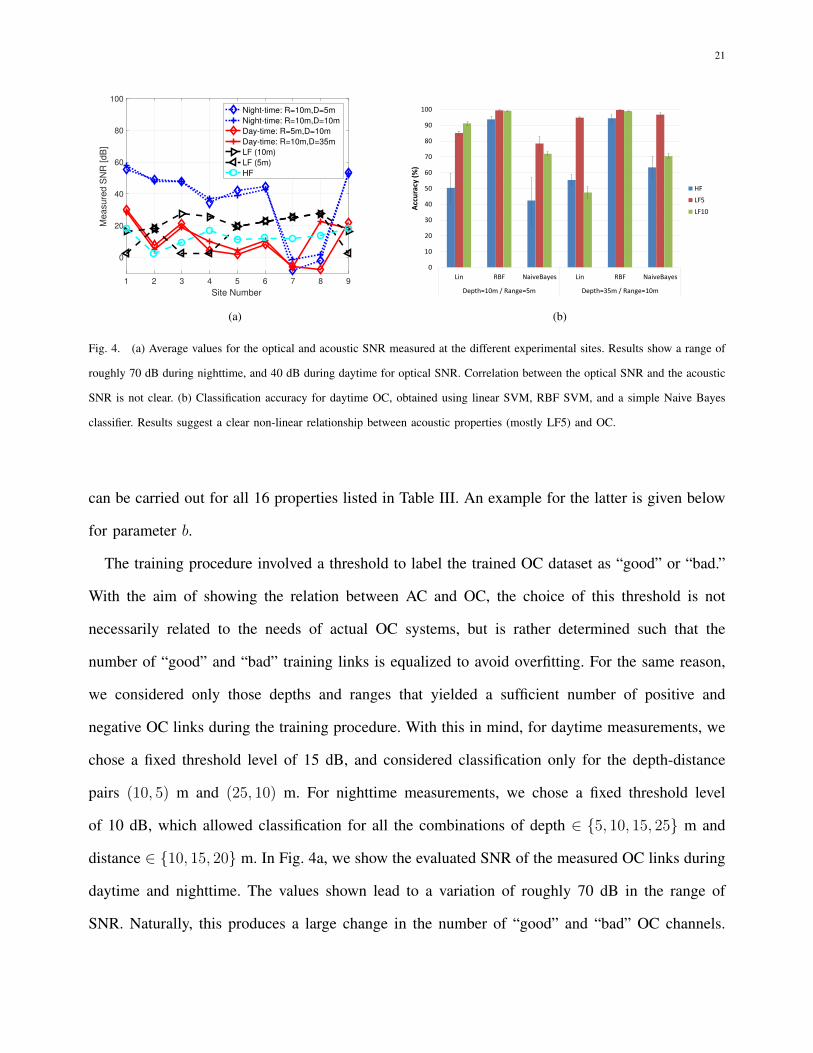
Fig. 4. (a) Average values for the optical and acoustic SNR measured at the different experimental sites. Results show a range of

roughly 70 dB during nighttime, and 40 dB during daytime for optical SNR. Correlation between the optical SNR and the acoustic

SNR is not clear. (b) Classification accuracy for daytime OC, obtained using linear SVM, RBF SVM, and a simple Naive Bayes

classifier. Results suggest a clear non-linear relationship between acoustic properties (mostly LF5) and OC.

can be carried out for all 16 properties listed in Table III. An example for the latter is given below

for parameter b.

The training procedure involved a threshold to label the trained OC dataset as “good” or “bad.”

With the aim of showing the relation between AC and OC, the choice of this threshold is not

necessarily related to the needs of actual OC systems, but is rather determined such that the

number of “good” and “bad” training links is equalized to avoid overfitting. For the same reason,

we considered only those depths and ranges that yielded a sufficient number of positive and

negative OC links during the training procedure. With this in mind, for daytime measurements, we

chose a fixed threshold level of 15 dB, and considered classification only for the depth-distance

pairs (10, 5) m and (25, 10) m. For nighttime measurements, we chose a fixed threshold level

of 10 dB, which allowed classification for all the combinations of depth ∈ 5, 10, 15, 25 m and

distance ∈ 10, 15, 20 m. In Fig. 4a, we show the evaluated SNR of the measured OC links during

daytime and nighttime. The values shown lead to a variation of roughly 70 dB in the range of

SNR. Naturally, this produces a large change in the number of “good” and “bad” OC channels.

22

More specifically, the choice of these threshold levels yielded on average a ratio between “good”

and “bad” channels of 62% for daytime and 65% for nighttime. Note that thresholding is required

only for classification. For regression, instead, the whole dataset was used to train the system and

predict the SNR of OC.

Training was performed separately for the acoustic LF recordings at 5 m, the acoustic LF

recordings at 10 m, and the acoustic HF recordings (10 m). The aim of training was twofold: 1)

discriminating the corresponding quality of the optical signal (binary-valued classification task),

and 2) predicting the corresponding optical values (real-valued regression task). To that end, the

dataset was first divided into training sets (75% of the patterns) and test sets (25% of the patterns),

and the latter were used to test the generalization capability of the models. We considered two

kernel functions: the simple linear SVMs, and the non-linear RBF kernel. To set the learning

hyperparameters, we adopted a k-fold cross-validation procedure, where one fold was randomly

selected and left out to test the current settings of the hyperparameters. Based on the amount of

available data, we used 3 folds for LF at 5 m, 4 folds for LF at 10 meters, and 5 folds for HF.

To evaluate the robustness of our approach and to reduce the risk of overfitting, each SVM was

trained 10 times, and we report the mean classification accuracy and the corresponding standard

deviations.

C. Classification results

The classification accuracy for the test sets is reported in Fig. 4b for both the linear SVM and

the non-linear SVM with the RBF kernel. We explore classification using all three types of acoustic

measurements. In all cases, the marked difference between the linear SVM and the RBF kernel

suggests that the relation between the acoustic properties and the optical link quality is non-linear.

In order to better assess the robustness of the findings, as a control simulation we also performed

the same classification task using a Naive Bayes classifier [44]. The average accuracy obtained

using this alternative type of algorithm was closely aligned with that obtained with the linear SVM

(see Figure 4b). For this reason, in the following experiments we only considered the SVM models.

23

Range=10m Range=20m Range=15m

0

10

20

30

40

50

60

70

80

90

100

Lin RBF Lin RBF Lin RBF Lin RBF Lin RBF Lin RBF Lin RBF Lin RBF Lin RBF Lin RBF Lin RBF Lin RBF

Depth=5m Depth=10m Depth=20m Depth=35m Depth=5m Depth=10m Depth=20m Depth=35m Depth=5m Depth=10m Depth=20m Depth=35m

Acc

ura

cy (

%)

HF

LF5

LF10

Fig. 5. Nighttime optical SNR. Results suggest a clear non-linear relation between acoustic properties and OC.

Moreover, overall the results indicate that the LF measurements provide a more accurate prediction

of the quality of the optical link, approaching 100% of classification accuracy for the non-linear

SVM. The LF measurements yield a much higher accuracy also for the linear SVM, except for

the condition corresponding to a depth of 35 m and a range of 10 m, where the performance of

LF10 is similar to that obtained using HF.

The classification accuracy for the test sets to predict the optical SNR during nighttime is reported

in Fig. 5. Here, many more values of optical SNR can be predicted. Also in this case, the non-linear

kernel clearly outperforms the linear SVM, achieving 100% for all the target properties. In fact,

for many properties, the performance of the linear SVM in Fig. 5 is close to chance level (50%).

Similar to the case of daytime optical transmission, in the nighttime scenario the LF measurements

(LF5 in particular) are better predictors for the quality of the optical link. However, when using

the linear SVM, HF sometimes still outperforms LF10, especially for the conditions corresponding

to long distances (range = 20 m). This suggests that in nighttime conditions the HF signal can

be more reliable than in daytime conditions, approaching a prediction accuracy of 100% for the

non-linear SVM and of 80% for the linear SVM at long ranges.

The high classification accuracy obtained for both the daytime and the nighttime prediction

of the quality of the optical link suggests a strong relationship between the acoustic properties

and the OC quality. This relation seems to be non-linear, as the greatest accuracy is achieved

24

TABLE IV

PRECISION, RECALL AND SPECIFICITY VALUES FOR ALL THE CLASSIFICATION TASKS.

Range (m) Depth (m)

Linear SVM Non-linear RBF kernel

HF LF5 LF10 HF LF5 LF10

Prec Recall Specif Prec Recall Specif Prec Recall Specif Prec Recall Specif Prec Recall Specif Prec Recall Specif

Daytime 5 10 0.37 0.38 0.58 0.76 0.93 0.79 0.88 0.95 0.87 0.93 0.90 0.96 0.99 0.99 1.00 0.99 0.99 0.99

10 35 0.53 0.40 0.70 0.57 0.97 0.95 0.27 0.44 0.49 0.96 0.92 0.96 1.00 0.96 1.00 0.98 0.99 0.99

Nighttime

10

5 0.75 0.51 0.39 0.96 0.85 0.77 1.00 0.91 0.96 0.99 0.99 0.97 1.00 1.00 0.98 1.00 1.00 0.98

10 0.76 0.51 0.31 0.96 0.85 0.79 0.99 0.92 0.94 0.99 0.99 0.97 1.00 1.00 0.97 1.00 1.00 0.98

20 0.82 0.46 0.21 0.96 0.85 0.81 0.99 0.92 0.92 1.00 1.00 1.00 0.99 1.00 0.97 1.00 1.00 0.99

35 0.83 0.42 0.14 0.96 0.85 0.77 0.99 0.92 0.92 1.00 1.00 1.00 1.00 1.00 0.98 1.00 1.00 0.99

15

5 0.81 0.74 0.32 0.37 0.21 0.59 0.52 0.45 0.45 0.98 0.98 0.95 0.99 1.00 0.99 0.99 1.00 0.98

10 0.80 0.72 0.39 0.96 0.87 0.78 0.83 0.82 0.46 0.99 0.99 0.96 1.00 1.00 0.97 0.99 1.00 0.96

20 0.76 0.72 0.25 0.40 0.23 0.61 0.49 0.38 0.49 0.99 0.99 0.96 0.99 1.00 0.99 0.98 1.00 0.98

35 0.84 0.45 0.29 0.96 0.84 0.80 1.00 0.92 0.97 1.00 1.00 1.00 1.00 1.00 0.99 1.00 1.00 0.98

20

5 0.79 0.80 0.48 0.58 0.86 0.45 0.64 0.92 0.44 0.96 0.96 0.89 0.99 1.00 0.99 0.98 1.00 0.98

10 0.51 0.67 0.42 0.57 0.87 0.43 0.21 0.36 0.49 0.95 0.95 0.95 0.99 1.00 0.99 0.99 0.94 0.99

20 0.84 0.85 0.65 0.99 1.00 1.00 0.24 0.39 0.52 0.99 0.99 0.98 0.94 1.00 1.00 0.96 1.00 0.99

35 0.84 0.87 0.59 0.98 0.99 1.00 0.25 0.40 0.56 0.99 0.99 0.98 0.97 1.00 1.00 0.96 1.00 0.99

by the SVM using the RBF kernel. In order to better evaluate the classifier performance across

different conditions, three additional performance measures were also computed from confusion

matrices [45]: precision (i.e., class agreement of the data labels with the positive labels given by

the classifier), recall (i.e., effectiveness of the classifier to identify positive labels), and specificity

(i.e., effectiveness of the classifier to identify negative labels). The complete results are reported in

Table IV. Precision, recall and specificity values are consistent across conditions, and fully aligned

with the accuracy results reported in Fig. 4b and Fig. 5. In particular, results show that indeed the

non-linear classifier achieves much better performance on all metrics, and has no biases for any

particular class.

Interestingly, the data seem to suggest that linear classification using LF measurements improves

close to the surface. This needs to be investigated further, as not all collected data shows this

same trend, and we have no further evidence to prove it. However, we still conjecture that linear

classification might be in fact more precise near the surface. A possible explanation can be a

high concentration of biological particles such as plankton in the upper water layer, which would

25

0

5

10

15

20

25

30

35

40

45

50

Lin RBF Lin RBF Lin RBF Lin RBF Lin RBF Lin RBF Lin RBF Lin RBF Lin RBF Lin RBF Lin RBF Lin RBF Lin RBF Lin RBF Lin RBF Lin RBF

5m 10m 20m 35m 5m 10m 20m 35m 5m 10m 20m 35m 5m 10m 20m 35m

Pre

dic

tio

n e

rro

r (d

B)

HF

LF5

LF10

10m 20m 15m

Depth =

Range = 5m

Fig. 6. Prediction error for the daytime optical SNR. Compared to the range of optical SNR, results suggest a good non-linear

prediction of the optical link quality from the acoustic properties.

scatter the acoustic wave and, during daytime, also sunlight. The collection of additional data in

this specific scenario would be a necessary step to verify this conjecture.

D. Prediction results

Classification results show evidence of a relationship between acoustic properties and optical

link quality. The strength of this relationship can be evaluated by prediction. The optical SNR

prediction errors for the test sets for all the 16 range-depth pairs of the daytime optical data are

reported in Fig. 6. Refer to Fig. 4a for the true optical SNR values at the different sites and for

daytime and nighttime data collection. The results are given in terms of the root mean squared error

(RMSE), measured in dB, for each type of AC dataset. As observed in the classification results,

the non-linear kernel outperforms the linear SVM when predicting SNR. Notably, the RMSE of

optical SNR achieved by the non-linear SVM is always around or below 5 dB at any measured

depth when the range is 5 m. Contrary to the classification task, using HF acoustic data to train

the RBF SVM for regression yields, in most cases, results that are better than those achieved using

LF acoustic data. This result might be due to the fact that the binary classification task is easier to

perform than the fine-grained regression task, which could be more challenging to fulfill at high

26

accuracy. The larger number of samples in the LF dataset might have introduced noise that was

detrimental only for the fine-grained predictions performed with the non-linear SVM.3

The optical SNR measured at several depths and ranges as well as the average measured acoustic

SNR values are shown in Fig. 4a. No clear correlation is visible at this point between the optical

and acoustic SNR values for the different testing sites. The optical SNR varies between –10 dB

and 60 dB for nighttime OC, and between –10 dB and 30 dB for daytime OC. Within such broad

ranges, being able to predict the optical SNR based on acoustic SNR measurements within roughly

5 dB of RMS error strongly suggests the existence of a relationship between AC and OC. We also

observe that the accuracy of the prediction decreases with increasing range, and is lowest for the

longest range of 20 m. Such a range is akin to the maximum operational range of several practical

underwater optical modems. Therefore, the accuracy decrease is expected, and mainly due to the

SNR decrease as a result of absorption and scattering of light power in water.

For the nighttime scenario, the prediction errors of the test sets for all the 16 range-depth pairs

are reported in Fig. 7. Similar to the case of daytime optical transmission, we observe that the

non-linear kernel operates far better than the linear one. When using RBF, the regression results

obtained using the HF dataset are better than those obtained using LF5 and LF10, which might be

due to overfitting. Although this trend was observed also in daytime conditions, this difference is

much more marked in nighttime conditions.

We now consider optical-SNR prediction accuracy as a function of depth. By analyzing the

trends in Fig. 7, we observe that for the RBF kernel, the prediction error at a fixed distance (i.e.,

for each different range) gradually decreases with depth. Hence, the optical signal becomes more

predictable as we move deeper in the water. However, this interesting trend holds only for the

first three depths, while at a depth of 35 m we notice that the prediction error remains about the

3Another possible explanation is that the HF regression training was overfitting the results. We have found a marked difference

between an accuracy of 0.5 dB in training and 2 dB in testing that may support this, where on the contrary, the LF error was

comparable between training and test sets. However, since the test performance of the non-linear SVM using HF was often lower

than that obtained with LF, this explanation is not supported by sufficient evidence.

27

0

5

10

15

20

25

30

35

40

45

50

Lin RBF Lin RBF Lin RBF Lin RBF Lin RBF Lin RBF Lin RBF Lin RBF Lin RBF Lin RBF Lin RBF Lin RBF Lin RBF Lin RBF Lin RBF Lin RBF

5m 10m 20m 35m 5m 10m 20m 35m 5m 10m 20m 35m 5m 10m 20m 35m

Pre

dic

tio

n e

rro

r (d

B)

HF

LF5

LF10

10m 20m 15m

Depth =

Range = 5m

Fig. 7. Prediction error for nighttime optical SNR. Compared to the range of optical SNR, results suggest a good non-linear

prediction of the optical link quality from the acoustic properties.

same or slightly increases. This phenomenon occurs for prediction using both LF and HF acoustic

measurements, and means that, up to a certain depth, the optical SNR becomes more predictable.

We argue that this effect is due to the scattering coefficient b which decreases with depth up to a

certain value, as seen in Fig. 3b. As long as b decreases, the exponential parameter in (15) becomes

less dominant, and predicting the optical SNR becomes easier. Note that this effect appears even

if the actual value of b cannot be predicted accurately per se. In order to test this hypothesis, we

trained the RBF SVM to predict the observed parameter b. The results shown in Fig. 8 imply that

it is harder to predict the value of b at a depth of 35 m. The reason behind this is that scattering

tends to happen mostly in the euphotic zone of the water column, whose boundaries are limited to

specific water depths. When optical measurements are performed deeper than the euphotic zone, b

tends to drop, as observed, e.g., from Station 7 data in Fig. 3b. Such a drop may not be captured

by the training over the rest of the data set, which explains the RMSE increase in Fig. 8 at a depth

of 35 m. Remarkably, this does not greatly affect the accuracy of the SNR prediction, because a

lower b also means that the SNR would be less affected by the exponential parameter in (15).

E. Impact of single properties on prediction accuracy

28

0.00

0.02

0.04

0.06

0.08

0.10

0.12

Depth=5m Depth=10m Depth=20m Depth=35m

RM

SE

HF

LF10

Fig. 8. RMSE for the prediction of the scattering parameter b using

the RBF SVM kernel.

We now wish to explore if there are

certain acoustic properties which are more

closely related to the optical properties and

are thus more informative for optical channel

quality prediction. We therefore investigate

the influence of each individual acoustic

property on the prediction accuracy of the

optical SNR. To that end, in this section,

instead of performing prediction based on the full set of nine (LF) and six (HF) acoustic properties,

we perform prediction based on each of the measured properties independently.

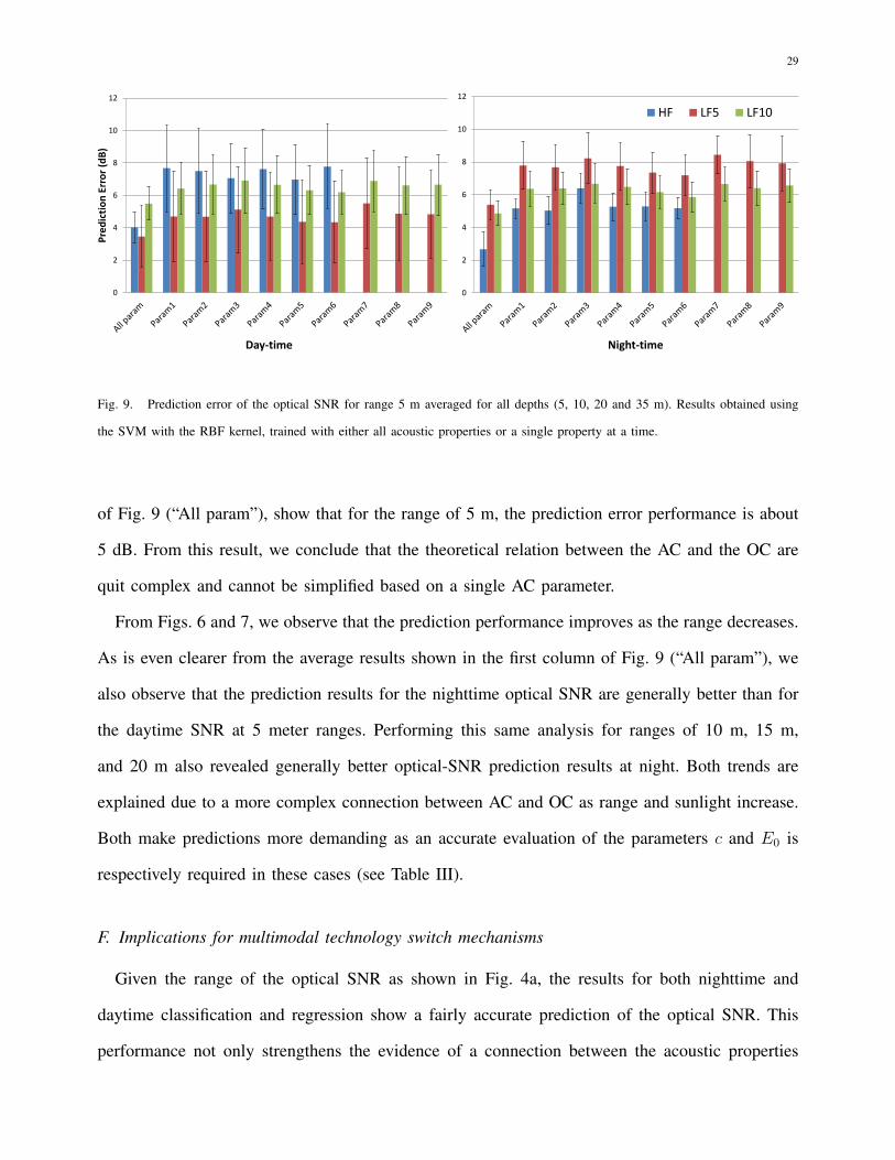
In Fig. 9, we show the daytime and nighttime prediction error of the optical SNR, respectively,

evaluated for a transmission range of 5 m, and averaged across the four considered depth values.

The enumerated properties match those in Table II. As expected, the average prediction accuracy

decreases when using only a single acoustic property as the predictor. For the nighttime case, this

result is observed when using both the lower and the higher frequency acoustic properties. However,

for regression of the optical SNR during daytime, this performance decrease is mostly observed

when using the HF data, and the decrease when using the LF data is only marginal. Compared

with the prediction performance when using all properties (column “All param” in Fig. 9), we note

that the prediction error increases only by roughly 3 dB. This result suggests that even when not

all considered acoustic properties are available, the relationship between AC and OC is sufficiently

marked to allow the prediction of the optical SNR. (Recall the intuitive explanation for this result

given in Section II-C.)

From Fig. 9, we observe that the average error is fairly constant across all single acoustic

properties. This suggests that the acoustic properties used have a similar correlation with the

optical properties. That is, no specific acoustic parameter is dominant for predicting the SNR of

the optical link. Yet, exploiting the whole set of parameters yields better performance, as the

prediction error decreases from 5–8 dB to 3–5 dB. In particular, the first set of bars in each panel

29

0

2

4

6

8

10

12P

red

icti

on

Err

or

(dB

)

0

2

4

6

8

10

12

HF LF5 LF10

Day-time Night-time

Fig. 9. Prediction error of the optical SNR for range 5 m averaged for all depths (5, 10, 20 and 35 m). Results obtained using

the SVM with the RBF kernel, trained with either all acoustic properties or a single property at a time.

of Fig. 9 (“All param”), show that for the range of 5 m, the prediction error performance is about

5 dB. From this result, we conclude that the theoretical relation between the AC and the OC are

quit complex and cannot be simplified based on a single AC parameter.

From Figs. 6 and 7, we observe that the prediction performance improves as the range decreases.

As is even clearer from the average results shown in the first column of Fig. 9 (“All param”), we

also observe that the prediction results for the nighttime optical SNR are generally better than for

the daytime SNR at 5 meter ranges. Performing this same analysis for ranges of 10 m, 15 m,

and 20 m also revealed generally better optical-SNR prediction results at night. Both trends are

explained due to a more complex connection between AC and OC as range and sunlight increase.

Both make predictions more demanding as an accurate evaluation of the parameters c and E0 is

respectively required in these cases (see Table III).

F. Implications for multimodal technology switch mechanisms

Given the range of the optical SNR as shown in Fig. 4a, the results for both nighttime and

daytime classification and regression show a fairly accurate prediction of the optical SNR. This

performance not only strengthens the evidence of a connection between the acoustic properties

30

and the optical ones, but also implies that the practical application of directing an autonomous

underwater vehicle (AUV) to the optimum range and depth for OC is realistic. That is, the AUV

can head directly to a location predicted to have good optical SNR, while still being deep enough

and far enough from the vessel it communicates with for safety reasons. In this context, the mission

of the AUV will be to communicate optically when in range, by keeping a safe distance to the

communicating vessel.

For a target optical SNR, Th, the following algorithm can be applied:

1) Train an acoustic-optical classifier and predictor based on collected data (the database openly

shared with this paper);

2) Collect acoustic properties to form an input data set;

3) Given range and depth, classify the quality of OC and predict the optical SNR, SNRo(r, d);

4) Direct the AUV to a location at range r and depth d for which OC is classified as a good

link, and for which SNRo(r, d) > Th, and switch from AC to OC.

V. CONCLUSIONS

In this work, we explored the statistical relationship between the properties of underwater

acoustic and optical links for the purpose of classifying the underwater optical link and predicting its

SNR. We based our analysis on a large database including both optical and acoustic measurements,

collected in nine different sea environments during a 13-day expedition. Our results indicate a clear

relation between the acoustic properties and the quality of the optical link. In particular, using the

RBF classifier, with the acoustic measurements we were able to predict the quality of the optical

link with an accuracy close to 100%. Moreover, for the range of 5 m, we were able to predict the

SNR of the optical link with an accuracy of about 5 dB within a dynamic range of 70 dB. Our

results further show that in most cases, the higher frequency measurements of the acoustic channel

can better predict the optical channel. Our classification and prediction algorithms can already serve

as a switching mechanism for multimodal systems that combine underwater acoustic and optical

communications. While our results provide strong evidence about the connection between acoustic

31

and optical channels in the water, we could not develop the mathematical relation between the

two channels, and this requires further exploration. As an additional future research direction, we

plan to include an initial unsupervised phase, which might discover useful patterns in the data and

thereby better support multiple supervised tasks. As a future direction, unsupervised learning, e.g.,

deep belief networks [46], [47], may discover other useful patterns in the data such as meaningful

clustering of the data, and that can adaptively set the classification thresholds. Successful application

of these approaches to communication systems [48], [49] motivates their use in our context as well.

ACKNOWLEDGMENTS

This work was supported by the EKOE (Environmental Knowledge and Operation Effectiveness)

program of the NATO STO Centre for Maritime Research and Experimentation (CMRE). The

dataset was acquired with projectors and hydrophone instruments from the anti-submarine warfare

(ASW) program of CMRE. We would like to thank the captain and the crew of NRV Alliance for

their kind assistance during data collection operations at sea.

REFERENCES

[1] X. Lurton, An introduction to underwater acoustics - Principles and applications. Springer Praxis, 2002.[2] Q. H. Davide Anguita, Davide Brizzolara, “Optical wireless underwater communication for AUV: Preliminary simulation and

experimental results,” in Proc. MTS/IEEE OCEANS, Santander, Spain, Jun. 2011.[3] R. Urick, Sound propagation in the sea. Peninsula Publishing Newport Beach, 1982.[4] B. Katsnelson, V. Petnikov, and J. Lynch, Fundamentals of shallow water acoustics. Springer Science & Business Media,

2012, ch. 3, 4.[5] F. Jensen, W. Kuperman, M. Porter, and H. Schmidt, Computational Ocean Acoustics, 2nd ed. New York: Springer-Verlag,

1984, 2nd printing 2000.[6] R. Spinrad, K. Carder, and M. J. Perry, Ocean Optics. Oxford Monographs on Geology and Geophysics. Oxford University

Press, USA, 1994.[7] F. Campagnaro, F. Favaro, F. Guerra, V. Sanjuan, M. Zorzi, and P. Casari, “Simulation of multimodal optical and acoustic

communications in underwater networks,” in Proc. MTS/IEEE OCEANS, Genova, Italy, May 2015.[8] “Free-falling optical profiler,” Last time accessed: Apr 2017. [Online]. Available: http://satlantic.com/profiler[9] “ac-9 plus,” Last time accessed: May 2016. [Online]. Available: http://www.electrotekintl.com/pdf/physical%20oceanography/

absorption%20and%20atteunation%20meter.pdf[10] F. Campagnaro, F. Guerra, R. Diamant, P. Casari, and M. Zorzi, “Implementation of a multimodal acoustic-optic underwater

network protocol stack,” in Proc. MTS/IEEE OCEANS, Shanghai, China, Apr. 2016.[11] N. Farr, A. Bowen, J. Ware, C. Pontbriand, and M. Tivey, “An integrated, underwater optical/acoustic communications system,”

in Proc. IEEE/OES OCEANS, Sydney, Australia, May 2010.[12] C. Cortes and V. Vapnik, “Support-vector networks,” Machine learning, vol. 20, no. 3, pp. 273–297, 1995.[13] M. Stojanovic and J. Preisig, “Underwater acoustic communication channels: Propagation models and statistical characteri-

zation,” IEEE Communications Magazine, vol. 47, no. 1, pp. 84–89, 2009.[14] M. Chitre, S. Shahabudeen, and M. Stojanovic, “Underwater acoustic communications and networking: Recent advances and

future challenges,” Journal of Marine Technology Society, vol. 42, no. 1, pp. 103–116, March 2008.[15] P. Casari and M. Zorzi, “Protocol design issues in underwater acoustic networks,” Elsevier Computer Communications, vol. 34,

no. 17, pp. 2013–2025, Nov. 2011.[16] J. G. Proakis, Digital Communications. New York, USA: 3rd ed. McGraw-Hill, 1995.

32

[17] K. G. Kebkal, O. Kebkal, and R. Petroccia, “Assessment of underwater acoustic channel during payload data exchange withhydro-acoustic modems of the S2C series,” in Proc. MTS/IEEE OCEANS, Genova, Italy, may 2015.

[18] R. Diamant, A. Feuer, and L. Lampe, “Choosing the right signal: Doppler shift estimation for underwater acoustic signals,”in ACM Conference on UnderWater Networks and Systems (WUWNet), Los Angeles, USA, Nov. 2012.

[19] R. Urick, Principles of underwater sound, 3rd ed. New York: McGraw- Hill, 1983.[20] M. Legg, A. Zaknich, A. Duncan, and M. Greening, “Analysis of impulsive biological noise due to snapping shrimp as a

point process in time,” in IEEE OCEANS, Aberdeen, Scotland, United Kingdom, june 2007.[21] C. Mobley, Light and water: radiative transfer in natural waters. Academic Press, 1994.[22] Y. Chen, X. Hu, D. Wang, H. Chen, C. Zhan, and H. Ren, “Researches on underwater transmission characteristics of blue-green

laser,” in Proc. MTS/IEEE OCEANS, Taipei, Taiwan, Apr. 2014.[23] F. Akhoundi, J. A. Salehi, and A. Tashakori, “Cellular Underwater Wireless Optical CDMA Network: Performance Analysis

and Implementation Concepts,” IEEE Transactions on Communications, vol. 63, no. 3, pp. 882–891, Mar. 2015.[24] “WFS Technologies,” Last time accessed: May 2016. [Online]. Available: http://www.wfs-tech.com/[25] X. Che, I. Wells, G. Dickers, P. Kear, and X. Gong, “Re-evaluation of RF electromagnetic communication in underwater

sensor networks,” IEEE Communications Magazine, vol. 48, no. 12, pp. 143–151, December 2010.[26] “S2CR 18/34 Acoustic Modem,” Last time accessed: February 2014. [Online]. Available: http://www.evologics.de/en/

products/acoustics/s2cr 18 34.html/[27] “Evologics S2C M HS modem,” accessed: Apr. 2017. [Online]. Available: http://www.evologics.de/en/products/acoustics/

s2cm hs.html[28] P. Minev, C. Tsimenidis, and B. Sharif, “Short-range optical OFDM,” in Proc. IEEE/OES OCEANS, Yeosu, Korea, May 2012.[29] L. Johnson, R. Green, and M. Leeson, “Hybrid underwater optical/acoustic link design,” in Proc. ICTON, Graz, Austria, Jul.

2014.[30] P. A. Forero, S. Lapic, C. Wakayama, and M. Zorzi, “Rollout algorithms for data storage- and energy-aware data retrieval

using autonomous underwater vehicles,” in Proc. ACM WUWNet, Rome, Italy, Nov. 2014.[31] S. Basagni, L. Booloni, P. Gjanci, C. Petrioli, C. A. Phillips, and D. Turgut, “Maximizing the value of sensed information in

underwater wireless sensor networks via an autonomous underwater vehicle,” in Proc. IEEE INFOCOM, Toronto, Canada,Apr. 2014, pp. 988–996.

[32] C. Moriconi, G. Cupertino, S. Betti, and M. Tabacchiera, “Hybrid acoustic/optic communications in underwater swarms,” inProc. MTS/IEEE OCEANS, Genova, Italy, May 2015.

[33] F. Campagnaro, F. Guerra, F. Favaro, V. S. Calzado, P. Forero, M. Zorzi, and P. Casari, “Simulation of a multimodal wirelessremote control system for underwater vehicles,” in Proc. ACM WUWNet, Washington, DC, Oct. 2015.

[34] R. Kastner, A. Lin, C. Schurgers, J. Jaffe, P. Franks, and B. S. Stewart, “Murao: A multi-level routing protocol for acoustic-optical hybrid underwater wireless sensor networks,” in Proc. IEEE SECON, Seoul, South Korea, Jun. 2012.

[35] V. N. Vapnik, “An overview of statistical learning theory,” IEEE Transactions on Neural Networks, vol. 10, no. 5, pp. 988–999,1999.

[36] A. J. Smola and B. Scholkopf, “A tutorial on support vector regression,” Statistics and computing, vol. 14, no. 3, pp. 199–222,2004.

[37] R. Diamant and L. Chorev, “Emulation system for underwater acoustic channel,” in International Undersea Defence TechnologyEurope conference (UDT), vol. 2, Amsterdam, the Netherlands, Jun. 2005, pp. 1043–1046.

[38] R. Diamant, “A normalized matched filter detector for hydroacoustic signals,” Elsevier Ocean Engineering, 2016.[39] “Beta function,” accessed: Apr. 2017. [Online]. Available: https://en.wikipedia.org/wiki/Beta function[40] M. Pal and P. Mather, “Support vector machines for classification in remote sensing,” International Journal of Remote Sensing,

vol. 26, no. 5, pp. 1007–1011, 2005.[41] G. M. Foody and A. Mathur, “Toward intelligent training of supervised image classifications: directing training data acquisition

for SVM classification,” Remote Sensing of Environment, vol. 93, no. 1, pp. 107–117, 2004.[42] John T. O. Kirk, Light and Photosynthesis in Aquatic Ecosystems, 3rd ed. Cambridge University Press, 2011.[43] M. Stojanovic, “Absorption and attenuation of visible and near-infrared light in water: dependence on temperature and salinity,”

Applied Optics, vol. 36, no. 24, pp. 6035–6046, Aug. 1997.[44] J. Huang, J. Lu, and C. X. Ling, “Comparing Naive Bayes, Decision Trees, and SVM with AUC and Accuracy,” in Third

IEEE International Conference on Data Mining, 2003. ICDM 2003. IEEE, 2003, pp. 553–556.[45] M. Sokolova and G. Lapalme, “A systematic analysis of performance measures for classification tasks,” Information Processing

& Management, vol. 45, no. 4, pp. 427–437, 2009.[46] G. E. Hinton, S. Osindero, and Y.-W. Teh, “A fast learning algorithm for deep belief nets,” Neural computation, vol. 18,

no. 7, pp. 1527–1554, 2006.[47] M. Zorzi, A. Testolin, and I. P. Stoianov, “Modeling language and cognition with deep unsupervised learning: a tutorial

overview,” Frontiers in Psychology, vol. 4, pp. 65–78, 2013.[48] M. Zorzi, A. Zanella, A. Testolin, M. De Filippo De Grazia, and M. Zorzi, “Cognition-based networks: A new perspective

on network optimization using learning and distributed intelligence,” IEEE Access, vol. 3, pp. 1512–1530, 2015.[49] A. Testolin, M. Zanforlin, M. De Filippo De Grazia, D. Munaretto, A. Zanella, and M. Zorzi, “A machine learning approach

to QoE-based video admission control and resource allocation in wireless systems,” in Ad Hoc Networking Workshop (MED-HOC-NET), 2014 13th Annual Mediterranean. IEEE, 2014, pp. 31–38.

RL – Paper-TW-Dec-16-1716.R1 – Page 1

Resubmission letter for manuscriptPaper-TW-Dec-16-1716.R1

“On the Relationship between the Underwater Acousticand Optical Channels”

Roee Diamant, Filippo Campagnaro, Michele De Filippo De Grazia, Paolo Casari,

Alberto Testolin, Violeta Sanjuan, Michele Zorzi

COMMENTS OF THE EDITOR

Comment E.1: The reviewer(s) have suggested some minor revisions to your manuscript.

Therefore, I invite you to respond to the reviewer(s)’ comments and revise your manuscript.

Answer: Thank you for your message. In the following we provide detailed responses to the

concerns raised by the reviewers.

RL – Paper-TW-Dec-16-1716.R1 – Page 2

COMMENTS OF REVIEWER 1

Comment 1.1: The reviewer has gone through the response and the revised paper, and has

no further comments.

Answer: Thank you for your assistance, and we appreciate your help with this manuscript.

RL – Paper-TW-Dec-16-1716.R1 – Page 3

COMMENTS OF REVIEWER 2

Comment 2.1: It is very good that the new results of classifier performance are provided.

Answer: Thank you for your kind words. Below we address the concerns you have raised.

Comment 2.2: 1) In Table IV, it is very good that the results of three metrics for evaluating

classifier performance are added. But in the results, the comma should be dot, since all

results are equal or less than 1. The comma is for separation of thousand.

Answer: Thank you for your close attention, and apologies for the confusion. In the revised

manuscript, we have corrected the table and replaced all commas by dots.

Comment 2.3: 2) Is it possible to establish mathematical model of some key parameters of

existing AC and OC large-scale fading channel? For the OC model, there are parameters of

scattering rate in equation (15). Can this parameter be related with the large scale fading

parameters of AC link? In Fig. 8, it is shown that the prediction of scattering parameter of

OC link by the data of AC link is effective. Can this be modeled by math?

Answer: We agree that a formal theoretical/mathematical model that relates the AC and OC is the

natural step forward. Unfortunately, due to the complexity of the physics of the two channels, we

were unable to find such a relation. Instead, we target our work to statistically show evidence that

this relation exists. We hope that our work will inspire further work in exploring the theory behind

the found relationship. In the revised manuscript, we have further clarified this in the abstract:

Due to the complexity of the acoustic and optical channels, we could not find the source of thiscorrelation. This work is therefore aimed to stimulate a theoretical study of the mutual properties ofunderwater acoustic and optical communication links.

Introduction section:

While we were unable to find a theoretical/mathematical explanation for the relation between the ACand the OC, we present statistical evidence that this relation exists. It is our hope to stimulate furthertheoretical investigations in this direction.

and in the Conclusions:

RL – Paper-TW-Dec-16-1716.R1 – Page 4

While our results provide strong evidence about the connection between acoustic and optical channelsin the water, we could not develop the mathematical relation between the two channels, and this requiresfurther exploration.

We would like to add that according to the results of Fig. 9, it appears that the relation between

the AC and the OC is complex. This is because, instead of a single AC parameter affecting the

SNR of the OC, it is evident that a combination of all parameters achieves the best prediction

results. In the revised text, we have clarified this by the addition text:

From this result, we conclude that the theoretical relation between the AC and the OC are quit complexand cannot be simplified based on a single AC parameter.

Comment 2.4: In Fig 9, the caption should be the “OC parameter prediction error,” not the

“OC SNR prediction error”.

Answer: Thank you for your close attention. Please note that in this figure, we show the prediction

error for the SNR of the OC. That is in contrast for the e.g., prediction error of the scattering

parameter b. In the revised manuscript, we have changed the caption into: “Prediction error of the

optical SNR ...”

Comment 2.5: From the results of Fig 7, Fig. 8 and Fig. 9, it can be concluded that, the AC

data of HF measurement working with the RBF kernel, provides the best prediction of OC

SNR and OC parameters in most cases. This finding can be added in the conclusion part.

Answer: Thank you for your suggestion. We have added this observation to the conclusions:

Our results further show that in most cases, the higher frequency measurements of the acoustic channelcan better predict the optical channel.

Comment 2.6: 5) In the explanation of AC/OC correlation, the main factors are the turbidity

of the propagation environment and the scatters in the underwater channel. Is it possible

that the turbidity and scatters be modeled mathematically? If you are able to establish these

models, the relationship between OC/AC results can be much clearer. However, due to that

the correlation of AC and OC are complicated as indicated in the results in figures, such

mathematical models are not mandatory for this paper.

Answer: The reviewer raises an interesting observation. The status of water turbidity affecting

optical communications is a local phenomenon influenced by large scale phenomena that take place

RL – Paper-TW-Dec-16-1716.R1 – Page 5

in the waters (e.g., turbidity currents that lead to the mixing of sea bottom sediments) and even

out of the water (such as the blowing of Saharian sands into the ocean, as was the case for Station

7 in this paper (see also Fig. 1). In the context of underwater optical communications, it is not

even the turbidity itself to be considered for channel modeling purpose, but rather its effect on the

attenuation of the power of a propagating optical wave. This is the meaning of the parameter b

considered in this paper. Being the nature of b that of a derived parameter, its modeling is quite

complicated, and to the best of the author’s knowledge there exists no statistical characterization

of its variation as a function of environmental parameters.

The main purpose of this paper, in fact, is not to investigate the mathematical characterization of

the influence of the underwater acoustic communications channel on the optical channel, but rather

to emphasize that there is a correlation between them, and that this correlation needs additional

investigation, as the impact of such a correlation on the design of underwater multi-modal opto-

acoustic communication nodes could be huge. We have further emphasized the above discussion

in the conclusions of the paper as follows:

While our results provide strong evidence about the connection between acoustic and optical channelsin the water, we could not develop the mathematical relation between the two channels, and this requiresfurther exploration.

RL – Paper-TW-Dec-16-1716.R1 – Page 6

COMMENTS OF REVIEWER 3

Comment 3.1: This is a very interesting paper on the relationship between underwater

acoustic and optical communications. It sheds light on the previously unexplored relationship

between these two communication methodologies and offers several practical applications that

could benefit from leveraging the relationships presented in this paper. The most important

contributions are the ability to use acoustic sensing of the water to classify the quality of the

optical link, either as good or bad, and to predict the optical link’s signal-to-noise ratio (SNR).

These contributions would directly benefit systems employing both sensing modalities (e.g.

autonomous underwater vehicles) by enabling efficient and optimal use of the two modalities.

This paper has improved very much from its original submission and from its second

submission. Importantly, the authors have satisfactorily improved explanations for results

presented and clarified concerns raised by reviewers in both iterations. There are still some

issues with clarity and conciseness; and there is a general difficulty in interpreting the

results (e.g. having to flip between text and figures on different pages). However, these

issues are minor and could potentially be corrected when the manuscript is reviewed for

page formatting. Based on the review guidelines for this journal, I recommend a minor

revision. If the minor revision conditions are met satisfactorily, this paper would be worthy

of acceptance.

Answer: Thank you for your summary and for your kind words. We apologize for the effort

required to follow text and figures on different pages. Since the structure of the paper may change

also due to IEEE editing, we prefer to fix the order of the figures and corresponding text at the

last step of paper formatting. In that phase, we will certainly pay close attention to your comment

about figure placement. In the following, we respond to the concerns you have raised.

Comment 3.2: Page 7; line 22: Replace “bigger then the laser one” with “larger than the

laser’s”

Page 7; line 24: Replace “holds much less” with “imposes fewer”

Page 7; line 26: Replace “Hamamatzu” with “Hamamatsu”

Page 19; line 13: Replace “transmitter” with “transmitter’s”

Answer: Thank you for your close attention. In the revised manuscript, we have corrected all

RL – Paper-TW-Dec-16-1716.R1 – Page 7

the above typos.