– 1 –

1. Nucleosynthetic Yields From Various Sources

In this section we discuss the various sites for producing the heavy elements, and give

a guide to the literature and to sources for the yields for each process. Talbot & Arnett

(1973, ApJ, 186, 69) defined a stellar production matrix, which describes the production

of each isotope in a star of initial mass m. One element of this matrix, Qij(m), represents

the fraction of the stellar mass which was originally present in the form of species j and

is eventually ejected by the star in the form of element i, so Qij(m) = (mej)ij(m)/(mXj),

where Xj is the abundance by mass of element j already present in the star when it first

formed.

Then the total contribution of a star of mass M to the ejected mass of the element i,

both newly formed, and originally present, is given by

(Mej)i =∑j=1,n

Qij(M) Xj M.

In most modern calculations, the yield for element i is given without the detail of what

was the initial form of i before nucleosynthesis, i.e. the production yield pim = (Mej)i/M .

The dependence on j is treated by carrying out the calculation of yields for various stellar

metallicities at each stellar mass.

Galactic yields yi are then the sum over a stellar generation with a specific IMF, taking

into account the minimum mass that dies (usually set to 1M⊙) and the remnants (white

dwarfs, neutron stars, black holes) for each species i.

Remember that the mass of a highly evolved star is its initial mass − mass lost during

evolution through winds. This early lost material has a chemical inventory close to or

identical to that of the star when it was formed. Then there is the mass ejected near

the end of the star’s lifetime (during the supernova, nova, etc), which will contain highly

– 2 –

processed material from the stellar interior as well as the outer layers of the star. Thus to

calculate the yields you need a detailed understanding of the last stages of stellar evolution,

of the explosion that might occur, and of the mass cutoff for ejection, as well as the nuclear

reaction network itself.

1.1. The Neutron Excess

Naively one might think that the nuclear reaction rates depend only on T , ρ, and the

initial chemical composition. But there is another important parameter, related to the

intitial chemical composition, the neutron excess.

Neutrons and protons can interconvert via weak interactions, and these conversions

occur during decays. The second reaction listed below, when only the right arrow holds, is

electron capture, while the third is β-decay.

p + ν ⇀↽ n + e+, p + e− ⇀↽ n + ν, n ⇀↽ p + e− + ν.

Free neutrons decay with a mean lifetime of ∼15 min via the last of the three reactions

listed above.

Depending on whether there is enough time for the various unstable isotopes that

may be produced to decay, one can end up with different isotopic compositions. This

is not only the case for the neutron capture processes, but also for nuclear reactions in

explosions, where the timescale may be so short that β-decays cannot happen. In addition,

the formation of neutron-rich isotopes, be they stable or unstable, is more rapid if there are

excess neutrons.

We must have a constant total number of nucleons. If weak interactions (decays)

– 3 –

cannot occur fast enough, we will have a constant number of protons and a constant number

of neutrons, Nn +Np =∑iNiAi, where Ai is the atomic mass of the isotope and the sum is

over all isotopes i present.

The neutron excess per nucleon, η, is (Nn −Np)/(Nn +Np). By charge neutrality, the

electron number is the total number of protons, and, since the material is fully ionized,

Ye =∑i YiZi, where Ye is the fraction of electrons in a fixed mass of the plasma and Zi is

the charge of each isotope i. By definition,∑i YiAi = 1, so one can show that η = 1− 2Ye.

Thus the neutron excess is related to a deficit of free electrons in the plasma.

Consider He burning in a convective core at T ∼ 108 K. 18O, with 8 protones and

10 neutrons, can be produced by 14N(α, γ)18F, followed by decay of 18F to 18O. This is

important because it converts a relatively abundant nucleus with no neutron excess (14N)

into a nucleus with a neutron excess of (2/18) = 0.111. For solar abundances, at this stage

of stellar evolution and nuclear processing in the core, this gives a total neutron excess of

η ≈ 1.5× 10−3.

Primordial gas is mostly H, which has only one proton, and no neutrons, and hence

the initial neutron excess is negative. As H burning proceeds, H is converted into 4He and

12C, both of which have a neutron excess of 0. Then, after He burning, η becomes slightly

positive as a small neutron excess builds up through production of 18O.

Since decays cannot happen during explosive nucleosynthesis (i.e. in modeling SNII),

the input neutron excess is identical to that of the final burned products that are eventually

ejected. Using the value η = 1.5× 10−3 in explosive nucleosynthesis calculations reproduces

the ratios of neutron-rich nuclei to their neighbors in the periodic table for the solar

composition. If a value significantly different is chosen, the predicted final isotopic ratios do

not match those for the Sun.

– 4 –

2. SNIa

SNIa are usually believed to be explosions of white dwarfs that have approached the

Chandrasekhar limit (Mch ∼ 1.39M⊙) through accretion from a companion in a binary

system, although in his recent colloquium Martin van Kerkwijk suggested a somewhat

different mechanism, the merging of two C-O white dwarfs. The white dwarfs are disrupted

by thermonuclear fusion of C and O from accreted material heated up by packing even

more accreted material on top of the white dwarf. Thus the details depend on the accretion

rate from the companion, among other parameters. Given these issues, SNIa yields are very

hard to calculate.

SNIa are used as standard candles in cosmology, and it therefore behooves us to

understand the explosion mechanism, and the resulting nucleosynthesis, well.

SNIa contribute very significantly to the Fe-peak elements. Their production of lighter

element is considerably less important. They produce very little of elements lighter than

Al. The first yield calculations were by Iwamoto, Brachwitz, Nomoto et al (1999, ApJS,

125, 439). Recently Travaglio, Hillebrandt, Reinecke & Thielemann (2004, A&A, 425, 1029)

present 2D and 3D hydrodynamical models of SNIa and a new set of nucleosynthesis yields.

The latest calculations of SNIa detonations are given by Woosley, Kerstein, Sankaran

& Ropke (2009, ApJ, 704, 255). These are deflagrations, a flame front of combustion

propagating at subsonic speeds through the transfer of heat, which may turn into

detonations (the same propagating at supersonic speeds). These flame fronts have a lot of

instabilities, making the calculations very difficult. They note that the Reynolds number

in a SNIa is orders of magnitude greater than any achieved in a terrestrial experiment or

numerical simulation due to the viscosity of electron-ion interactions in a fully ionized dense

plasma.

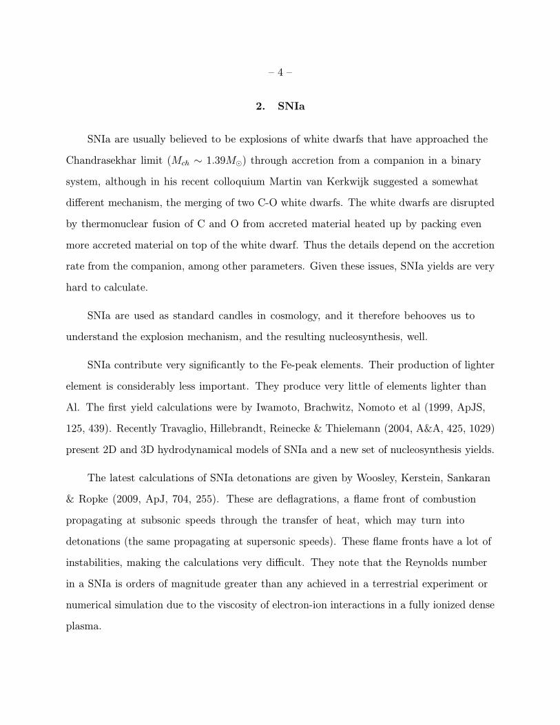
– 5 –

Fig. 1.— Mass fraction of a few major nuclei resulting from C-deflagration prediced by

Nomoto (Fig. 7a from Nomoto (1984, ApJ, 286, 644).

– 6 –

Fig. 2.— Fig. 9 from Travaglio et al (2004). The light elements are depleted relative to the

Solar mixture while the Fe-peak elements are strongly produced.

– 7 –

3. Core Collapse SN Yields

Core collapse SN are the end phase of evolution of massive stars in the range of 8 to

∼130M⊙. A single SN in the early galaxy can substantially enrich all the gas in the halo,

so understanding their yields is quite important. The yields depend on the mass of the

progenitor, the amount of mass loss during normal stellar evolution, the explosion energy,

the mass cutoff (mass above the cutoff is ejected, that below settles into the remnant, a

black hole), mixing around the cutoff area, and the mass of 56Ni produced. Since it is

so difficult to model SN, with so much poorly understood physics, that noone can make

one explode in a computer, these calculations are tuned by matching the characteristics

of observed SN, including of course SN1987A in the LMC. From the observed light curve

and spectral fitting of individual SN, the explosion energy and produced 56Ni mass can be

determined.

Unlike SNIa, the core collapse family of SN is very diverse in their characteristics,

luminosity, spectra (some show hydrogen lines, others no H, but strong He, others neither H

nor He, presumably depending on the amount of mass lost prior to the explosion), explosion

energy, etc. Most models are spherically symmetric, but that may not match reality.

Currently three varieties are recognized: very energetic hypernovae, with kinetic energy

about 10 times larger than normal SNII, i.e. > 1052 ergs, which probably form black holes

as remnants, normal core collapse SN with explosion energy ∼ 1051 ergs, and very faint and

low energy SN, which may be characterized by a lot of fall-back so that most of the Fe ends

up in the black hole rather than being ejected. Their progenitors were probably at the low

end of the mass of the core-collapse SN family.

In addition to enriching the ISM, these energetic events have strong dynamical and

thermal influences on the ISM, discussed in the section on feedback. The relationship of

core-collapse SN to GRBs is another area of great current interest.

– 8 –

Two burning regions, incomplete and complete Si-burning, dominate the nucleosynthesis

production. The latter, at Tpeak > 5 × 109 K, produces large amounts of Co, Zn, V, and

Cr; the former produces Cr and Mn. Both produce 56Ni, which eventually becomes 56Fe.

The details depends on the neutron excess, which in turn depends on the metallicity, and

in particular affects the production of the odd atomic number Fe-peak elements, i.e. Mn

and Co, hence the odd-even effect. A high explosion energy enhances the α-rich freezeout

(see the section in the notes on nuclear reaction rates regarding late stages of evolution in

massive stars), hence the production of Zn and Co.

Several groups calculate yields for these SN. One is led by Ken Nomoto in Japan and

another by Stan Woosley at UC Santa Cruz. The first major set of calculations was by

Woosley & Weaver (1995, ApJS, 101, 181), while some of their latest yields are given in

Heger & Woosley (2009, ApJ, see arXiv:0803.3161).

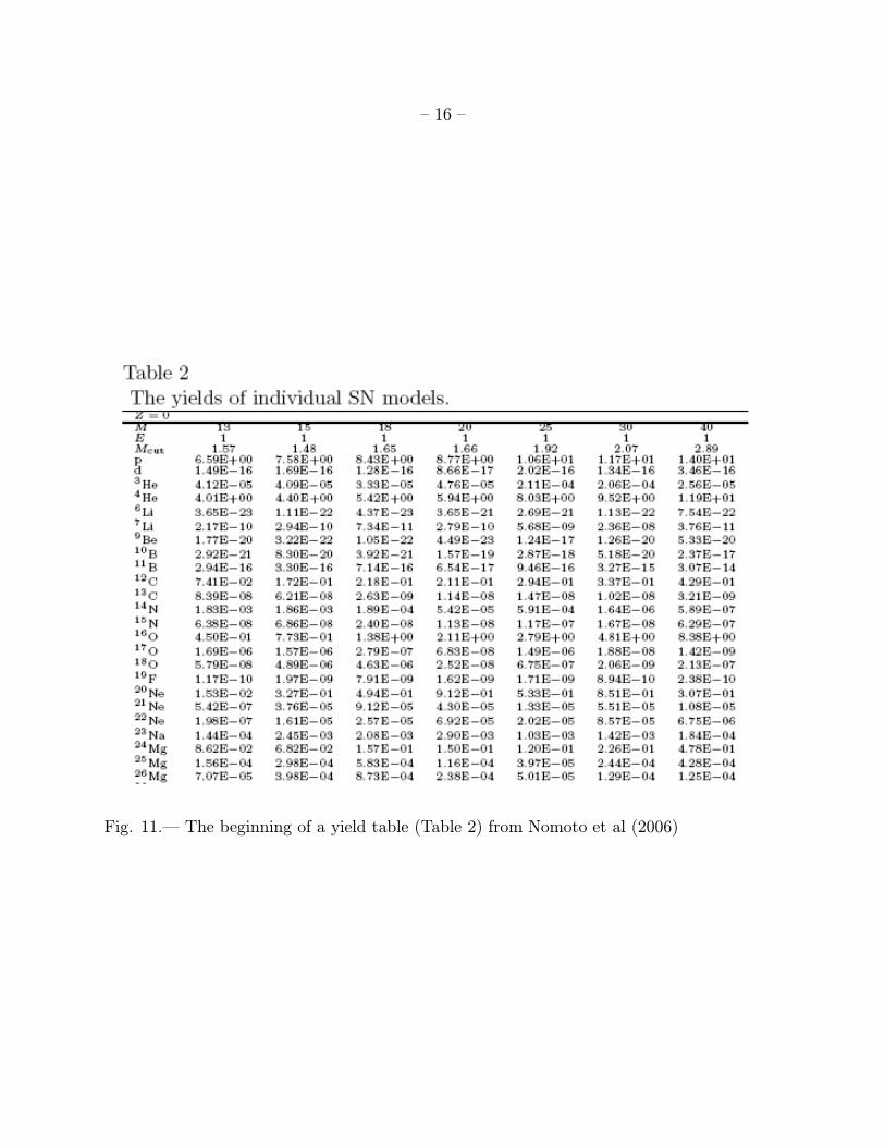
Nomoto, Tominaga, Umeda, Koayashi & Maeda (2006, Jrl. Nuc. Phys. A777, 424) is a

good summary of the work of the Japanese group. Table 2 of their paper give the detailed

yields (mass in units of the Solar mass) in the ejecta for each isotope a function of inital

stellar mass and metallicity. Table 3 gives the IMF weighted yields as well.

The Italian Group have also published yields for core collapse SN, see their latest set

given in Chieffi & Limongi (2004, ApJ, 608, 405). Note that no elements above Zn are

produced by any mass in their grid up to a metallicity of ∼ 10−3 that of the Sun. That is

true of calculations by other groups as well.

– 9 –

Fig. 3.— Fig. 1 from Hamuy & Suntzeff, 1990 (AJ). Light curves in various optical

bandpasses for SN 1987A in the LMC.

– 10 –

Fig. 4.— Fig. 5 from Hamuy & Suntzeff, 1990 (AJ, 99, 1146). Light curves of the absolute

visual magnitude for a number of SNII with data extending to more than 100 days, including

SN 1987A. Note that from day 130 to 400, all the SNII fall with roughly the same exponential

rate of decline. Compared to the very large variation in intrinsic brightness near the peak

and during the first 100 days, the absolute V mags of the SNII after day 130 are remarkably

similar.

– 11 –

Fig. 5.— Lightcurve in 3 optical colors for SN1998bw showing the exponential decay at

late times expected if the energy input is from a radioactive unstable element produced in

the SN explosiont and then ejected. This is believed to be copiously produced 56Ni, which

decays in 6 days to 56Co, which decays in 77 days to 56Fe. The observed decay half life is

∼50 days, which is that expected for 56Co as modified by the effect of expansion of the shell,

and leakage of gamma rays. Fig. 1 of McKenzie & Schaefer, 1999, PASP, 111, 964.

– 12 –

Fig. 6.— Fig. 1 from Nomoto et al (2006)

– 13 –

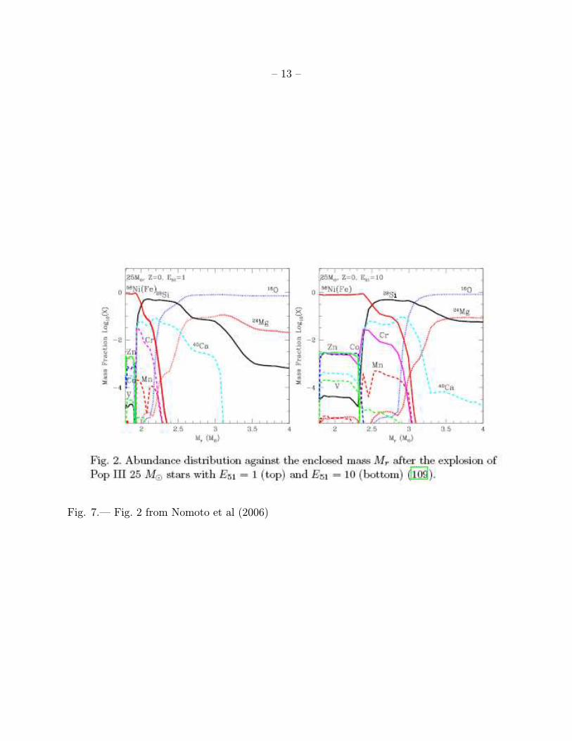
Fig. 7.— Fig. 2 from Nomoto et al (2006)

– 14 –

Fig. 8.— Fig. 3 from Nomoto et al (2006)

– 15 –

Fig. 9.— Table 1 from Nomoto et al (2006)

Fig. 10.— Fig. 11 from Nomoto et al (2006)

– 16 –

Fig. 11.— The beginning of a yield table (Table 2) from Nomoto et al (2006)

– 17 –

3.1. Pair Instability SN Yields

Extremely massive stars with initial M > 140M⊙, if such exist, have oxygen cores

which exceed Mc = 50M⊙. These can reach very high temperatures at relatively low

densities. Conversion of energetic photons into electron-positron pairs occurs prior to

oxygen ignition. The gas is largely radiation pressure supported, so when this happens and

the radiation pressure drops abruptly, a violent contraction triggers a catastrophic nuclear

explosion whose energy unbinds the star completely, leaving no remnant at all. Until very

recently, there has been no detected PISN in all of the very many active and past SN

searches. Thus it was believed that if PISN acutally occur, they would be confined to the

early Universe, where 0 metallicity would permit such high mass stars to be formed and to

evolve.

Such stars, if present, would be tremendously important in chemical evolution because

of the very large amount of ejected material. Their nucleosynthesis, first worked out in detail

in Heger & Woosley (2002, ApJ, 567, 532) (look for their cases where 140 < M/M⊙ < 260),

is characterized by an extremely large odd-even effect, far larger than that observed in any

known Galactic star, suggesting that even in the early Universe, PISN were rare or absent.

More than 50M⊙ of56Ni can be formed during the collapse, but no elements beyond Zn

are produced as there are no neutron capture processes. An interesting alternative view is

presented by Karlsson, Johnson & Bromm (2008, ApJ, 679, 6) who claim to be able to hide

PISN ejecta in a clever way.

The first detection of a PISN was recently claimed by Gal-Yam, Mazzali, Ofek et al

(2009, Nature, 462, 624), SN 2007bi, whose host is a dwarf galaxy with mass about 1% that

of the Milky Way, presumably of low mean metallicity. They claim that based on the high

extremely luminosity of this SN at peak, and the slow rise time to peak, that the kinetic

energy released was ∼ 1053 ergs, the exploding core mass is likely to be ∼100M⊙, and that

– 18 –

more than 3M⊙ of56Ni was synthesized. They thus infer that SN 2007bi must have been a

PISN.

Somewhat lower mass stars may become pulsational pair instability SN, suggested for

stars in the mass range 95 to 130M⊙ by Woosley, Blinnikov & Heger (2007, Nature, 450,

390). The scenario proceeds as above, but in this case, the energy released by the explosive

burning is inadequate to unbind the star, which ejects many solar masses of surface material

in a series of giant pulses.

– 19 –

Fig. 12.— Fig. 2 from Umeda & Nomoto, 2002, Conference proceeding, Astro-ph/0205365).

Note the different vertical scale in the two panels. The odd-even effect is about 100 times

larger in the PISN than in the hypernova.

– 20 –

Fig. 13.— The light curve for SN 2007bi, the PISN candidate identified by Gal-Yam, Mazzali,

Ofek et al (2009, Nature, 462, 624). The light curve follows the 56Co decay rate. The lower

light curve is that of SN 1987A in the LMC multiplied by a factor of 10 in luminosity.

– 21 –

4. Asymptotic Giant Branch Stars

AGB stars represent the last nuclear burning phase for stars with initial masses from

about 0.8 to 8M⊙. AGB nucleosynthesis was first discussed in detail by Renzini & Voli

(1981, A&A, 94, 175), as part of an effort to explain the luminosity and frequency of carbon

stars in the LMC and in the SMC. Such stars are believed to contribute significantly to

the light elements, and also be the dominant site for production of the heavy s-process

elements. The latter requires some contortions, mixing fresh unburned H into regions in

which H has already been burned into He, to produce 13C, which then produces neutrons to

operate the s-process. This is believed to happen as a result of a series of He shell flashes

at intervals of ∼104 yr in a star burning H and He in separate narrow shells. See Busso,

Gallino & Wasserburg (1999, ARA&A, 37, 239) for a detailed discussion of the operation of

the s-process in AGB stars.

The s-process is metallicity dependent in the sense that Fe-peak nuclei are needed as

seeds for producing the rare heavier nuclei. Then, since these stars do not explode, but

rather lose mass by surface winds, the processed material from the center must be mixed

upward in the star close enough to the surface that convection zones can bring the material

to the surface, where it can be spread into the ISM by the stellar wind. Eventually, after

between 15 and 100 flashes, the star becomes pulsationally unstable, and the mass loss rate

becomes very high, terminating the AGB phase.

Only species that can be produced by H and He burning are produced in AGB stars.

AGB stars, through internal processing, burn O into Na, Mg into Al, and carbon into

nitrogen. They produce the rare isotopes of Mg (25,26Mg).

The key species for which AGB stars make important contributions are C, N, O, 19F,

23Na, 31P (the only stable isotopes of the odd atomic number elements F, Na and P)

and specific isotopes of abundant elements formed in low abundance in standard stellar

– 22 –

nucleosynthesis, including 25,26Mg (most Mg is 24Mg), and 30Si (only 3% of Solar Si, Si is

92% 28Si in the Sun), as well as the heavy s-process neutron capture elements.

Although AGB yields are low, and the amount of material per AGB star returned to

the ISM is not large, there are many more AGB stars in a stellar population with a typical

IMF than there are SN of any kind. Thus the cumulative effect on the chemical inventory

of a galaxy from AGB stars can be large for specific species.

Amanada Karakas and John Lattanzio have been working on this issue. Karakas

(2010, MNRAS, arXiv:0912.2142) gives her latest tabulation of yields, updating those

given by Karakas & Lattanzio (2007). The new yields are given as electronic tables

in their recent paper; their earlier yields from their 2007 study can be found online at

www.mso.anu.edu.au/∼akaraks/stellar yields. Calculation of these yields requires a deep

understanding of stellar evolution, and mixing, and many poorly known parameters must

be specified. Among these is the mass loss rate that is assumed.

The yields from Karakas (2010) are given for a set of 15 values of the stellar mass from

1 to 6.5M⊙, and for metallicity from 1/200 Solar to the Solar value (4 metallicities) as

online tables, where they define the yield for species i as

Mi =∫ τ0

[Xi −X0(i)]dM

dtdt,

Mi is in solar masses, dM/dt is the current mass loss rate, Xi and X0(i) are the current and

initial mass fraction of species i, and τ is the total lifetime of the stellar model. If the yield

is negative, the species is destroyed, if the species is produced, the yield is postitive.

The head of one such table is given below as an example. The last column in the table

is the production factor f = log[Xi/X0(i)].

Other recent calculations of AGB star yields include those of Stancliffe & Jeffery (2007,

– 23 –

MNRAS, 375, 1280) and Ventura & D’Antona (2009, A&A, 499, 835). The differences

among them appear to be due to differences in the stellar models, the treatment of

convection, etc.

– 24 –

Fig. 14.— Fig. 2 from Karakas (2010).

– 25 –

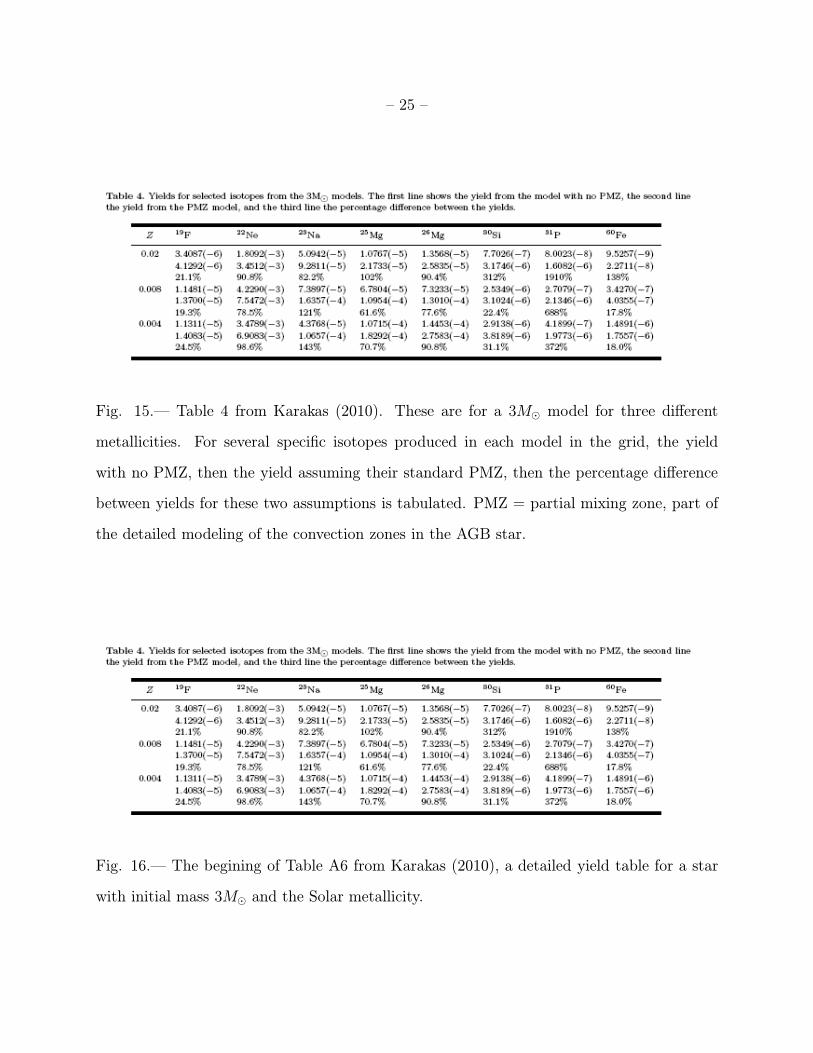
Fig. 15.— Table 4 from Karakas (2010). These are for a 3M⊙ model for three different

metallicities. For several specific isotopes produced in each model in the grid, the yield

with no PMZ, then the yield assuming their standard PMZ, then the percentage difference

between yields for these two assumptions is tabulated. PMZ = partial mixing zone, part of

the detailed modeling of the convection zones in the AGB star.

Fig. 16.— The begining of Table A6 from Karakas (2010), a detailed yield table for a star

with initial mass 3M⊙ and the Solar metallicity.

– 26 –

Fig. 17.— The begining of Table 2 from Ventura & D’Antona (2009), a detailed yield table.

Note the different definition of the tabulated quantity from those tabulated by Karakas.

– 27 –

5. Novae

Nova explosions occur when a critical hydrogen rich envelope is reached on the white

dwarf component of the nova binary, by accretion from its low mass companion. There

is a thermonuclear runaway in the H rich envelope of a CO white dwarf. Novae occur

fairly frequently, perhaps 20 per year in our Galaxy. Unlike in a SNIa, the nova star is not

disrupted, it continues as a white dwarf in a binary system. Presumably, assuming mass

transfer continues, the nove explosion will recur.

There is a class called recurrent novae where the recurrence timescale is short enough,

perhaps 20 to 50 years, that multiple nova outbursts have been recorded for a particular

star. Schaefer, Pagnotta, Xiao et al (2010, arXiv:1004.2842) discuss the recurrent nova

U Sco, for which the tenth recorded eruption was observed earlier this year. It has outbursts

at intervals of about 10 years. They estimate the total mass accreted between eruptions by

integrating the energy emitted over that period from the light curve, and show that is is a

constant, which suggests a white dwarf with mass close to the Chandrasekhar limit, and a

high accretion rate.

Nova explosions are much less energetic than a SN; the ejection velocities are much

lower (∼ 1000 km/sec), the ejected mass is low (∼ 10−4M⊙), etc. Since nova outbursts

are often detected within our galaxy, we can watch the light curves as the ejecta cool, and

actually see dust formation in the ejecta in some cases.

Early calculations of the nuclear reactions that are expected to occur in novae were

given by Starrfield, Truran, Sparks & Arnould (1978, ApJ, 222, 600). A more recent

analysis of nova nucleosynthesis yields can be found in Gehrz, Truran, Williams & Starrfield

(1998, PASP, 110, 743). In particular, if the acreting donor star loses most of its envelope,

the material transfered can include partially burned H, in particular include 3He, and thus

novae can produce Li. Nova ejecta often contain large amounts of N and O, and novae also

– 28 –

produce the rare CNO isotopes.

Nova abundances are inferred from the emisison line spectra of their ejecta. Some

novae show large excesses of Ne. (See, e.g. Gehrz et al (2007, ApJ, 672, 1167, The Neon

Abundance in the Ejecta of QU Vul From Late-Epoch IR Spectra). It is believed that the

neon is not produced in the explosion itself, but rather results from mixing of material in

the CO core of the nova progenitor (the white dwarf itself) (which includes a lot of Ne)

with the accreted envelope. Jose, Hernanz, Garcia-Berro & Pons (2003, ApJL, 597, L41)

carry out some relevant modeling which supports this conjecture. This implies that there is

a minimum mass at which elements beyond CNO should be expected to be enhanced in the

nova ejecta, which is Mi ∼ 9.3 M⊙.

More on novae can be found in the lecture notes on The Physics of Classical Novae,

1990, Springer Verlag, Lecture Notes in Physics, 369, 138.

– 29 –

Fig. 18.— The Roche lobe and mass transfer in binary systems.

– 30 –

Fig. 19.— Huge enhancements of N and O, by factors of about 200 for N and 20 for O, in the

ejecta of Nova Cyg 2006, with Ne, Ar, and Fe normal, and H and He depleted compared to

Solar ratios. These were found by looking at emission lines arising from the ejected material.

(Table 9 of Munari, Siviero, Henden et al, 2008, A&A, 492, 145)