1

Multiscale Plasticity : Dislocation Dynamics H.M. Zbib, Washington State University\

-10000

-5000

0

5000

10000

V3

-5000-2500

02500

5000 V1

-5000

0

5000

V2

Effective Plastic Strain (%)

0.2531970.1740730.0949490.0158248

ta

dislocations

cracks

penny-shaped cracks

Ua

V

2

ContentsContents

1. Basic Geometry: Identification of Slip geometry (bcc), Discretization of dislocation curves

2. Equation of Motion: Glide, climb, cross-slip, multiplication

3. Long Range Stress Field and Driving Force

4. Short-range interactions

5. Boundary Conditions: periodic, reflected, free, etc..

B. Basic Structure of Dislocations Dynamics

C. Numerical issues: • Long-range Interactions: Superdislocations vs FEM• Time step and Segment length

D. Critical Issues _Examples

E. Movie (Typical simulations)

A. Basic Structure of The multi-scale model of Plasticity 1. Representative Volume Element: Inhomogeneous; homogeneous 2. Basic laws of continuum mechanics 3. Constitutive Laws: Connection with Dislocation Dynamics4. The Finite Element formulation5. Boundary Conditions: Dislocation-Boundary Interaction6. Extension to Heterogeneous materials

3

DSSST

Internal stress (caused by defects)

External Stress

pDee

Elastic strain caused by external stress

Elastic stress caused by internal defects

Inelastic strain

dvSD )(xV elementelement

DD 1

4

Dp SCS : Hooke’s Law:

Momentum: vSdiv pS.ε TkTcv

2Energy:

peo

ε-ε C= S S + S -SSo

pW -W=

Rate form

5

Interaction with External free surfaces:

The solution for the stress field of a dislocation segment is known for the case of infinite domain and homogeneous materials, which is used in DD codes. Therefore, the principle of superposition is employed to correct for the actual boundary conditions, for both finite domain and homogenous materials. ta

dislocations

cracks

penny-shaped cracks

Ua

V

t

V

ta-t

*

*uuu

SSS *

6

Internal surfaces:

Internal surfaces such as micro-cracks and rigid surfaces around fibers, say, are treated within the dislocation theory framework, whereby each surface is modeled as a pile- up of infinitesimal dislocation loops. Hence defects of these types are all represented as dislocation segments and loops, and there interaction with external free surfaces follows the method discussed above.

7

FE Formulations:

dvBCBK eT

V

s

aa dsNtf

s

II dsNtf

v

DB dvBSf

v

PeP dvBCf

Image stresses

Applied stress

Internal stress: Long range interactions

Shape Change

Stiffness Matrix

PBa ffffUKUM

TTT fTKTC

8

Extension to Inhomogeneous Materials and interfaces

1

2

T

1

2

T-T

1

12

2*

1*

**

CCS

"2" in,SCS

"1" inCS

uuuSSS

ˆ

ˆ

,

,

*

*

T1

Infinite domain with properties of material“1”

“Eigenstress”Elastic Strain field in domain“2” caused by dislocations in Domain “1” (infinite-domain solution)

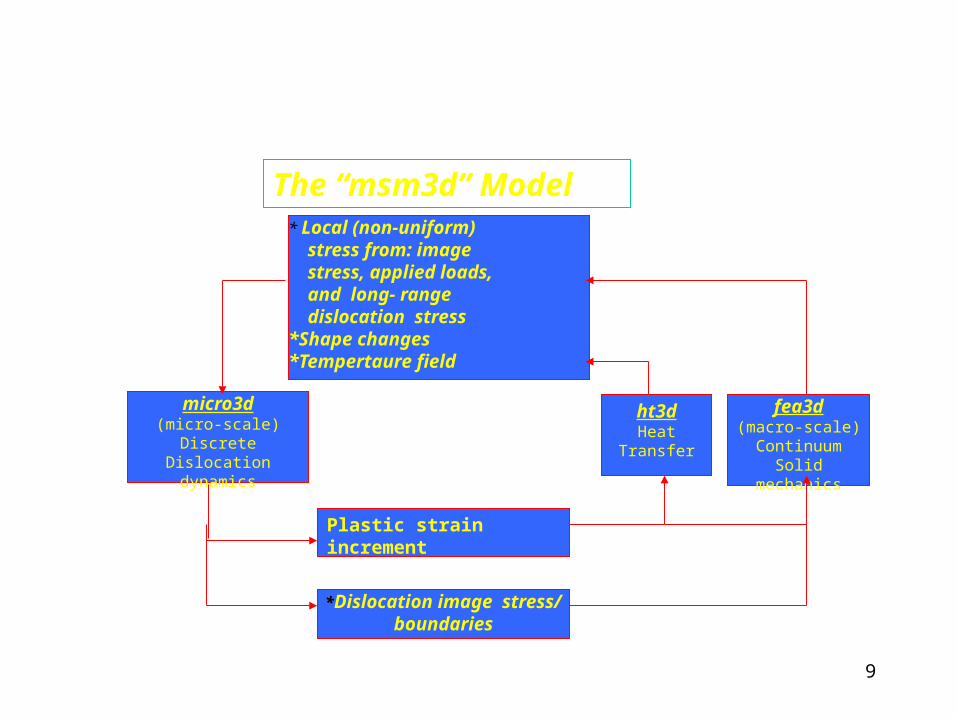
9

micro3d(micro-scale)

Discrete Dislocation dynamics

fea3d(macro-scale)

Continuum Solid mechanics

*Dislocation image stress/ boundaries

* Local (non-uniform) stress from: image stress, applied loads, and long- range dislocation stress*Shape changes*Tempertaure field

Plastic strain increment

ht3dHeat Transfer

The “msm3d” Model

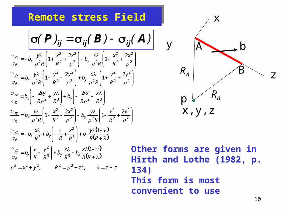
10

z

x

y A

B

b

x,y,zp

)()()( ABP ijijij

zzzRyx

RR

xb

R

xb

R

y

Rb

RR

yb

R

x

Rb

R

xb

x

R

x

R

yb

x

R

x

R

xb

R

x

R

xb

R

y

R

yb

y

R

y

R

xb

y

R

y

R

yb

x

R

x

R

xb

x

R

x

R

yb

zyxyz

zyxxz

yxxy

yxzz

yxyy

yxxx

,, 222222

33

2

0

3

2

30

2

2

2

2

22

2

2

2

20

32320

2

2

2

2

22

2

2

2

20

2

2

2

2

22

2

2

2

20

1

1

21

21

22

21

21

21

21

Other forms are given in Hirth and Lothe (1982, p. 134)This form is most convenient to use

RA

RB

Remote stress FieldRemote stress Field

11

3D Discrete Dislocation Dynamics3D Discrete Dislocation Dynamics

)nbbn( iiip

i

N

i

gii

V

vl

1 2

)nbbn(W iiip

i

N

i

gii

V

vl

1 2

ii vm *F

t

v

dv

dW

vm

1*

Equation of Motion

Effective Mass

12

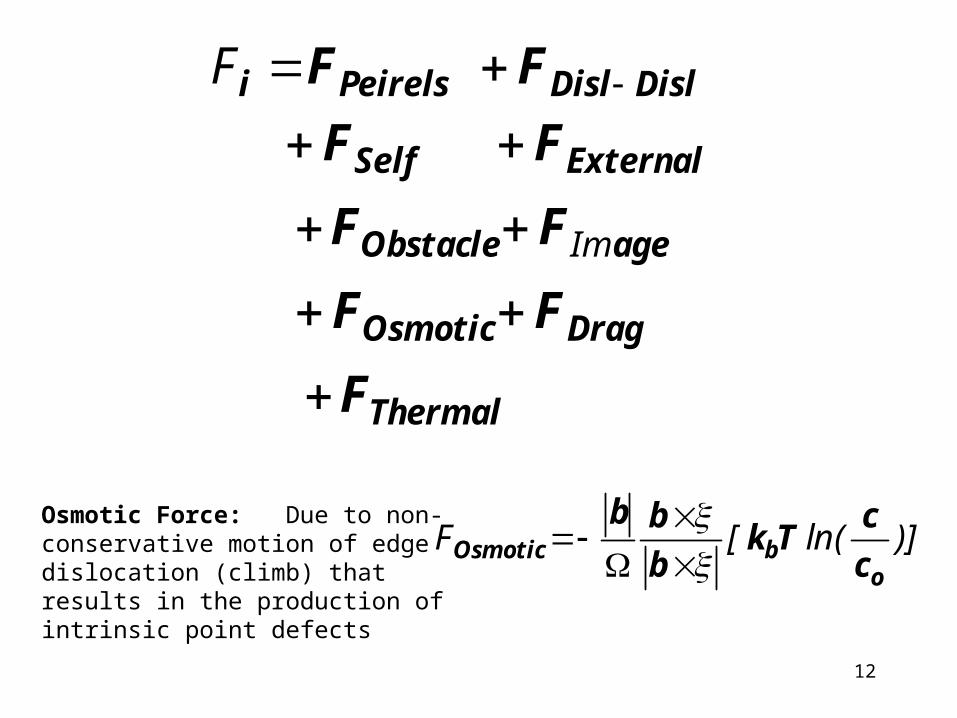
Thermal

DragOsmotic

ageObstacle

ExternalSelf

DislDislPeirelsi

F

FF

FF

FF

FF

Im

F

Osmotic Force: Due to non-conservative motion of edge dislocation (climb) that results in the production of intrinsic point defects

)]ln([Fo

bOsmotic c

cTk

b

bb

13

kT

F

kT

D

a

bhM kk

g

-exp

2 2

Double-Kink Theory(bcc: Low mobility)

Viscous Phonon and Electron damping

MB Tg

1

( )

fcc: High mobilitye.g AL: 1410 sPa.

Urabe and Weertman (1975)

14

Thermal Force - SDD: Stochastic Dislocation Dynamics

• Equation of motion of a dislocation segment of length Dl with an effective mass density m* (Ronnpagel et al 1993, Raabe et al 1998):

• the stochastic stress component t satisfies the conditions of ensemble averages

0)( tτ

• The strength of t is chosen from a Gaussian distribution with the standard deviation of

tlbBkT 22

T

10K 2 = 8.11MPa = 11.5 MPa

50 5 28.7 40.6

100 10 57.4 81.1

300 30 181 256 For Cu with = 50 fs

tlmbBkTttt 2*22)()( ττ

B bl 10 bl 5sPa.

t

iiThermal b τF

15

0

100

200

300

400

500

600

700

0 50 100 150 200t (ps)

Tk (

K)

SDD: Fluctuation of Kinetic Temperature

• Pinned dislocation with initial velocity = 0 m/s

• Total dislocation length = 2000 b & segment length =10b

• System temperature = 300 K, w/o applied stress

22

2KBTk

DOFMv

16

I. Basic Geometry (bcc)I. Basic Geometry (bcc)

Simulation Cell(5-20 )

[100] [010]

[001]

Slip plane

(101)

m b

Initial Condition: Expected outcome!*Random distribution Mechanical properties (yield stress, (dislocation, Frank-Read hardening, etc..). Pinning points (particles) Evolution of dislocation structures*Dislocation structures Strength, model parameters, etc..

Discrete segmentsof mixed character

“Continuum” crystal

17

Nodes and collocation points on dislocation loops and curves

“1”

“3”

P

Rjpj

j+1

j-1

dl’

C1

C2

C3

i

i+1

i-1i-2

jj+1

“2”

vj+1

vj

v

Field point

Velocity vector

 Long-range Stress field

kC

2

iαβ

βαi

3

imkm

α2

iCimβmβ

2

iCimαmαβ

xdRx

δxxx

Rb

ν)π(14

G

xdRx

bπ8

GxdR

xb

π8

G)(σ

p

18

}

{

k2

iαβ

βαi

3

imkm

α2

iimβmβ

2

iimαmαβ

xdRx

δxxx

Rb

ν)π(14

G

xdRx

bπ8

GxdR

xb

π8

G)(σ

1

111

1

j

j

j

j

j

j

n

jLoopsallp

N

j

Djjp

11,)(

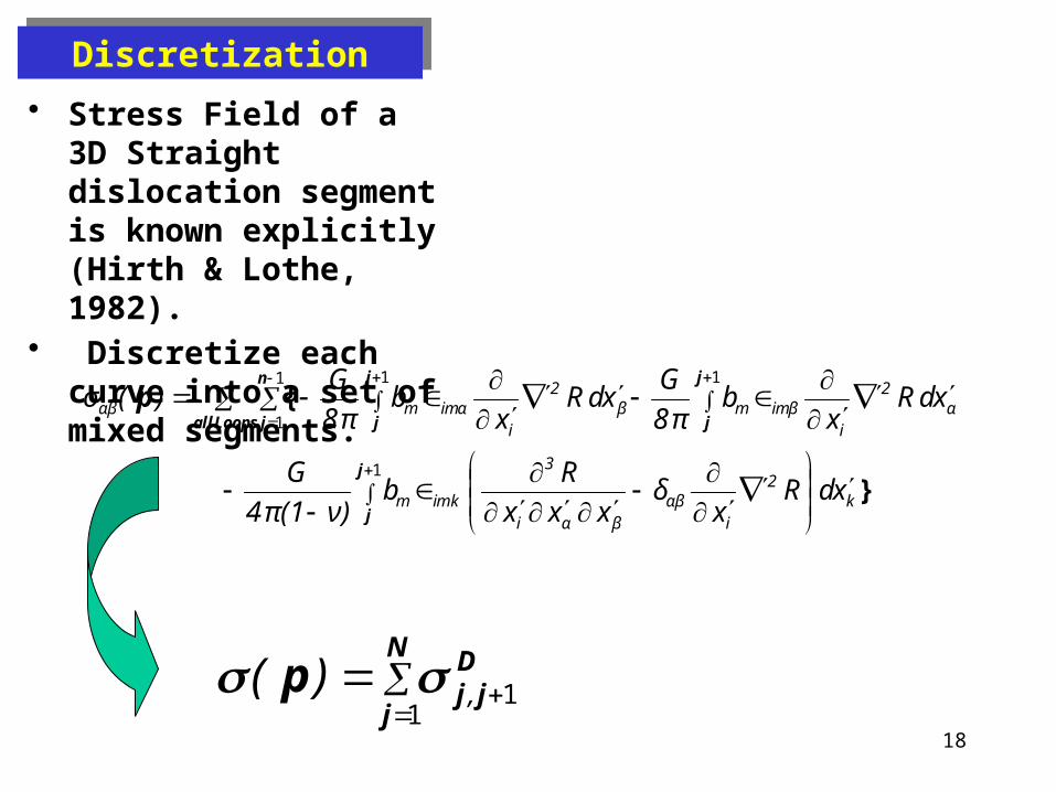
• Stress Field of a 3D Straight dislocation segment is known explicitly (Hirth & Lothe, 1982).

• Discretize each curve into a set of mixed segments.

DiscretizationDiscretization

19

z

x

y A

B

b

x,y,zp

)()()( ABP ijijij

zzzRyx

RR

xb

R

xb

R

y

Rb

RR

yb

R

x

Rb

R

xb

x

R

x

R

yb

x

R

x

R

xb

R

x

R

xb

R

y

R

yb

y

R

y

R

xb

y

R

y

R

yb

x

R

x

R

xb

x

R

x

R

yb

zyxyz

zyxxz

yxxy

yxzz

yxyy

yxxx

,, 222222

33

2

0

3

2

30

2

2

2

2

22

2

2

2

20

32320

2

2

2

2

22

2

2

2

20

2

2

2

2

22

2

2

2

20

1

1

21

21

22

21

21

21

21

Other forms are given in Hirth and Lothe (1982, p. 134)This form is most convenient to use

RA

RB

Remote stress FieldRemote stress Field

20

x

y

z

Identification of basic geometryIdentification of basic geometry

For each node identify:• Coordinates, • Burgers vector• slip plane index • neighboring nodes (k & j) • Node type (free, fixed, junction, jog,

boundary,etc.

“Basic Unit”

i(x,yz)

j

k

b

21

 

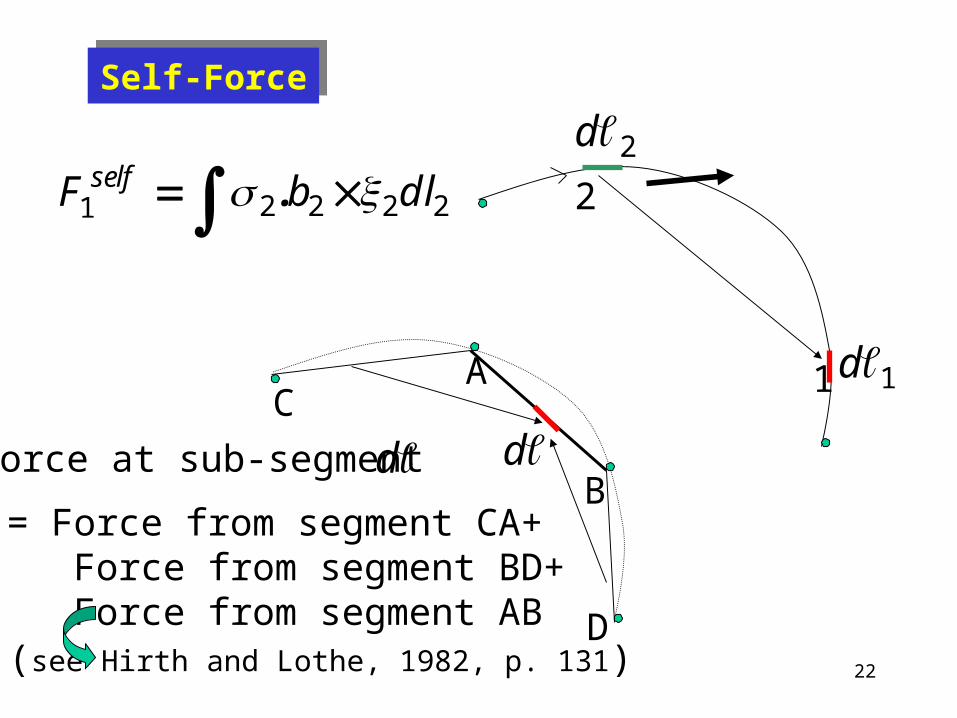
Self-force and Peach-Koehler Force at Dislocation Nodes

bi

i

Fi

i

22

1d

2d

22221 dlbF self . 2

1C

A

B

D

dForce at sub-segment d

= Force from segment CA+ Force from segment BD+ Force from segment AB

(see Hirth and Lothe, 1982, p. 131)

Self-ForceSelf-Force

23

CA

B

D

gF

DCAB

BDBACAg

FFbL

bfL

bfF

cossin

,,

211

14

44

A

ABb

zx

B

Explicit expression

Self-Force per unit lengthSelf-Force per unit length

24

1

1

1

1

ABz

CAx

A

AABy

CAy

ABx

CAx

ABz

CAzCA

bb

bbbbbbfsin

cos

Average force per unit length :

DCBDBACAg FF

Lnbfbf

LF

,,4

Cut-off parameter; numerical parameterwhich can be adjustedto account for core energy

• Similar expressions are obtained for the normal force.

• These expressions reduce to those given in Hirth and Lothe (1982, p.138) for

e.g.

CAAB bb

25

A

B

b

For pure edge pure screw dislocations, this reduces toe.g.

b

gF

gF

(force per unit length)

L

nL

bFg

4

2

Ln

L

bFg

41

1 2

26

Initial Configuration

x

y

z

Vb

II. Equation of MotionII. Equation of Motion

Nonlinear system of ODE’s

componentglideselfiii

N

j

aDjji

iii Fbvv

.....)(

p)(T,M

1m ,

* 1

11

i=1,…N

27

BCC:4 Burgers vectors, without regard to slip planes 8 possible distinct reactions,

-4 repulsive, 3 attractive, and one annihilation. When slip planes are considered: For the {110} and {112} planes 420 attractive reactions all of which are sessile (Baird and Gale, 1965)

d

A short-range interaction occurs when the distance “d” between two dislocations becomes comparable to the size of the core *annihilation, *formation of dipoles, *jogs, and *junctions.

Detailed investigation of each possible interaction can become very cumbersome

Short Range InteractionsShort Range Interactions

28

1. Critical distance criterion (Essman and Mughrabi, 1979)

Implicitly takes into account the effect of the local fields arising from allsurrounding dislocations.

Criteria for determining interaction:

Rule 1: If c

PK FF and PKF or changes sign as

the segment is advanced, short range interaction is possible provided that local interaction between segmentAB and its closest neighbor CD, CDABF is attractive

A

B

C

D

2. Force-based criterion:

29

Rule 2: If Rule 1 is satisfied and

1CDAB ξ.ξ and 0 CDAB bb (or 1CDAB ξ.ξ and 0 CDAB bb ),

AB and CD will annihilate by either

i. Glide (if they are on the same plane) or

ii. Cross slip (if they are on intersecting planes).

Annihilation

Free nodes

Frank-Read source

30

The probability that two attractive dislocationsform a jog or a junction is implicitly determinedby their interaction forces.

For example, if they were to form a junction, theinteracting segments rotate relative to each otherto align themselves into a configuration moresuitable for junction formation, yielding areduction in the energy.

If not, they form a jog since it is energeticallymore favorable

A

B

C

D

31

Rule 3: If Rule 1 is satisfied, andcjnCDAB with 0 CDAB bb ,

then a junction is formed.Segments AB and CD are combined toform a new segment at the junctionwhose Burgers vector is equal to .bb CDAB

Junction node

Junction

22

21

2bbbb 21

In a crude approximation, this implies that this reaction is energetically favorable.

Example:

bb

in

bb

in

A

B

3111 110

3111 110

[ ] ( )

[ ] ( )

[010]glide plane(100)

32

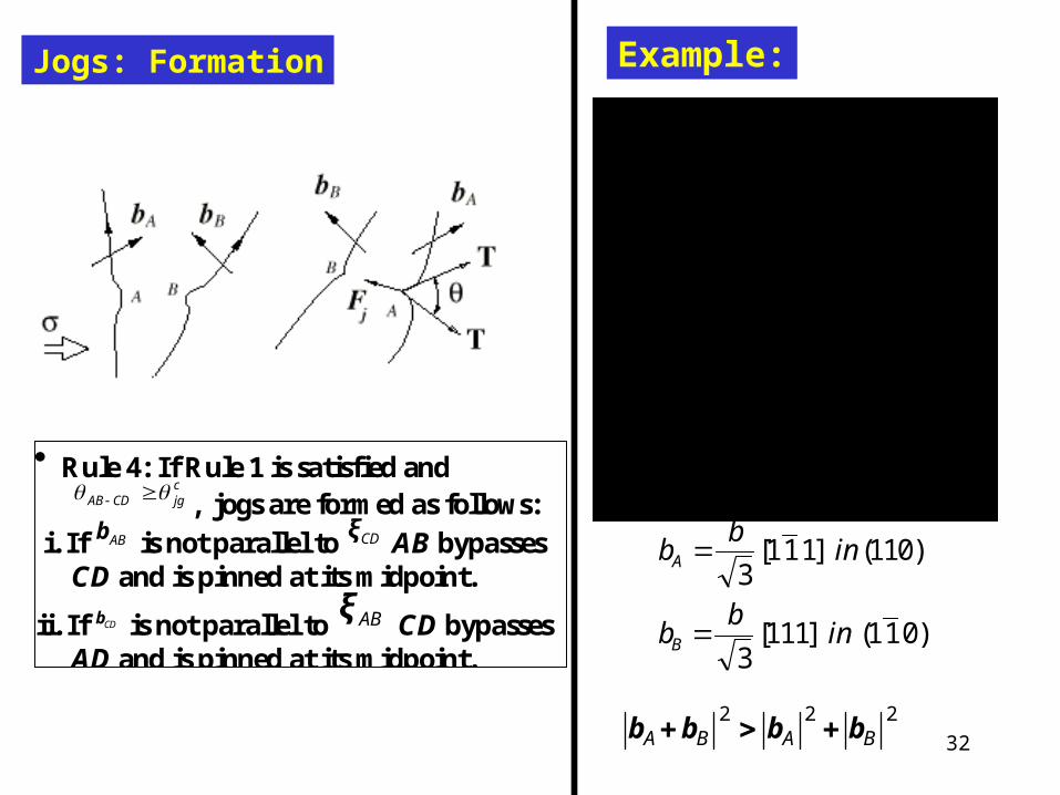
Rule 4: If Rule 1 is satisfied and

cjgCDAB , jogs are formed as follows:

i. If ABb is not parallel to CDξ AB bypasses CD and is pinned at its midpoint.

ii. If CDb is not parallel to ABξ CD bypasses AD and is pinned at its midpoint.

Jogs: Formation Example:

222BABA bbbb

bb

in

bb

in

A

B

3111 110

3111 110

[ ] ( )

[ ] ( )

33

32cos

b

Wvcjgs

ocjgs 120

For Ta:

Rule 5: If cjgsjg the jog moves forward in

the direction of average velocities of

the two adjacent dislocation segments.

Jogs: Motion

• Vacancy or interstitial generating jogs• Line tension approximation

Vacancy or interstitial formation energy

34

Dipole

Dipoles form naturally (numerically) without a need for a “Rule”.

35

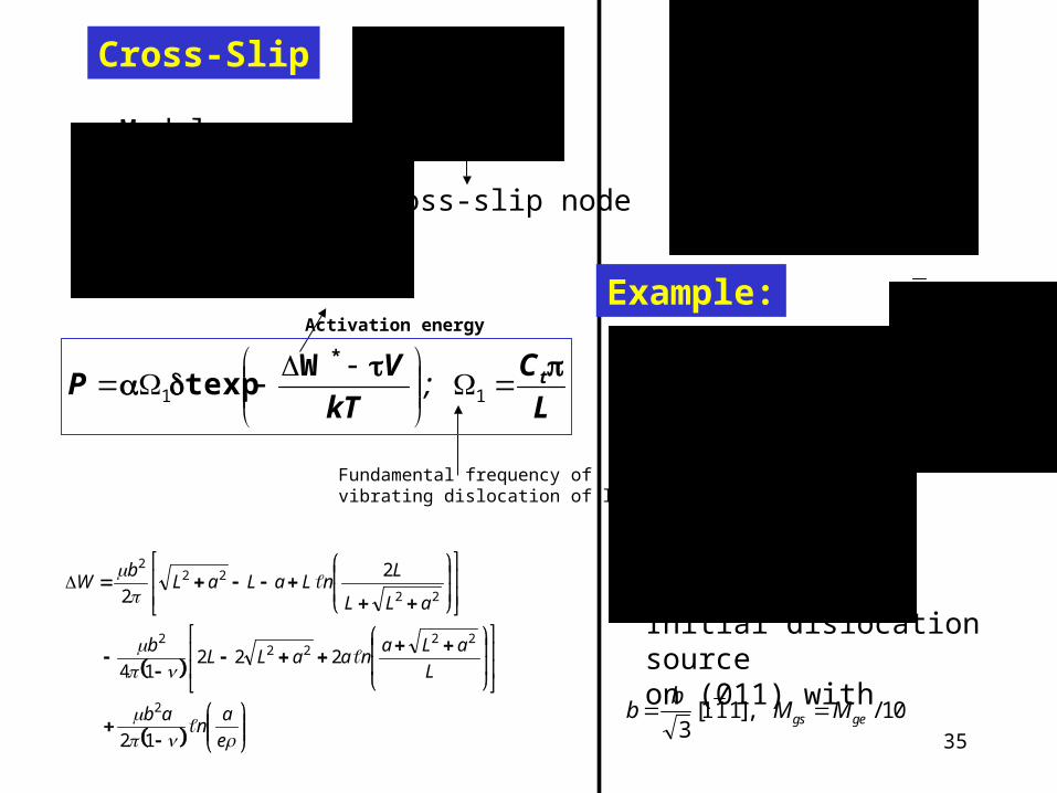
L

C

kT

VP t

11 ;

*Wtexp

Cross-Slip

e

an

ab

L

aLanaaLL

b

aLL

LnLaLaL

bW

12

22214

2

2

2

2222

2

22

222

Model

Activation energy

Cross-slip node

Example:

Initial dislocation sourceon (011) with

bb

M Mgs ge 3

111 10[ ], /

[ ]111 view

Fundamental frequency of vibrating dislocation of length L

36

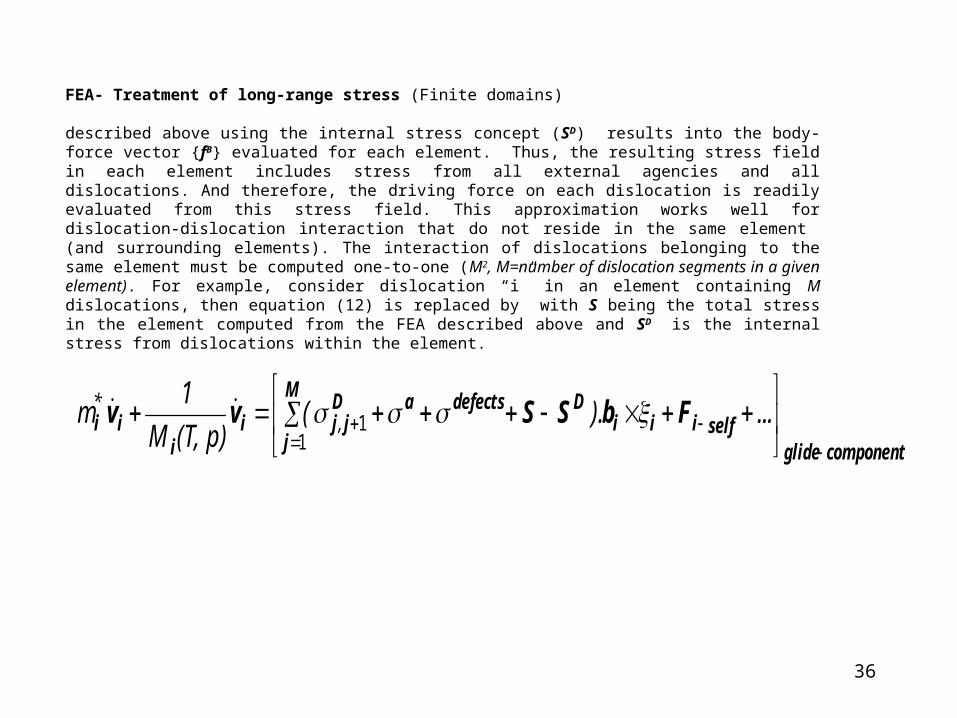
FEA- Treatment of long-range stress (Finite domains)

described above using the internal stress concept (SD) results into the body-force vector {fB} evaluated for each element. Thus, the resulting stress field in each element includes stress from all external agencies and all dislocations. And therefore, the driving force on each dislocation is readily evaluated from this stress field. This approximation works well for dislocation-dislocation interaction that do not reside in the same element (and surrounding elements). The interaction of dislocations belonging to the same element must be computed one-to-one (M2, M=number of dislocation segments in a given element). For example, consider dislocation “i” in an element containing M dislocations, then equation (12) is replaced by with S being the total stress in the element computed from the FEA described above and SD is the internal stress from dislocations within the element.

componentglideselfiii

M

j

DdefectsaDjji

iii FbSSvv

....)(

p)(T,M

1m ,

* 1

1

37

Infinite domainsBoundary conditions: Periodic, reflectedSuperdislocation (Long Range stresses)

Finite Domains: Boundary condition: Free, rigid, interfaces, mixed Image stresses: FEA

38

PZo

Q

A: Main Computational Cell(Grain)B,C, D.: Cells/Grains

C, or D Cell with N Dislocations

P: Dislocationin Cell A

Z

x

y

Main computaional Cell A is surrounded by MxM Cells (41x41)

39

Elements Involved

2.Sample Conditions

Creep – 10-4/s

Quasi-static Strain Rate

High Strain Rate: 103 108/s

rdefect = 1022~1024/m3 T = RT ~ 0.5 Tmelt

1.Defects & Materials

3.Simulation/ Coding Continuum/ Finite

Element Discrete Dislocation

Dynamics Thermal Fluctuations Nonlinearities Geometric Distortions

40

Material parameters 

Elastic properties Dislocation Mobility lawCore size = 1b Stacking-fault energy, & activation energy for cross-slip

Numerical Parameters:

DD Cell size (= FE mesh size)  Dislocation segment length (min (3b) and max) (variable), number of integration points (10)Number of cells (infinite domain; 3x3x3) Number of sub-cells (elements for FE)time step for DD; Max flight distance (variable time step )Time step for FE (dynamics) ~ (smallest dimension/shear speed)

kT

F

kT

D

a

bhM kk

g

-exp

2 2

MB Tg

1

( )

Double-Kink Theory

(bcc: Low mobility)

Viscous Phonon &

Electron damping