1 Molecular Simulation of Polymer Melts and Blends ... · Molecular Simulation of Polymer Melts and...

1Molecular Simulation of Polymer Melts and Blends: Methods,Phase Behavior, Interfaces, and SurfacesPeter Virnau, Kurt Binder, Hendrik Heinz, Torsten Kreer, and Marcus M€uller

1.1Introduction

Understanding thermodynamicproperties, including also thephasebehavior of poly-mer solutions, polymer melts, and blends, has been a long-standing challenge [1–7].Initially, the theoretical description was based on the lattice model introduced byFlory and Huggins [1–7]. In this model, a flexible macromolecule is represented by a(self-avoiding) random walk on a (typically simple cubic) lattice, such that each beadof the polymer takes one node of the lattice, and a bond between neighboring beadsof the chainmolecule takes a link of the lattice. For a binary polymer blend (A,B), twotypes of chains occur on the lattice (and possibly also �free volume� or vacant sites,whichwe denote asV ). Themodel (normally) does not take into account any disparityin size and shape of the (effective) monomeric units of the two partners of a polymermixture. Between (nearest neighbor) pairs AA, AB, and BB of effective monomers,pairwise interaction energies, eAA, eAB and eBB, are assumed. Thus, this model dis-regards all chemical detail (as would be embodied in the atomistic modeling [8–10],where different torsional potentials and bond-angle potentials of the two constituentscan describe different chain stiffness).

Despite the simplicity of this lattice model, it is still a formidable problem ofstatistical mechanics, and its �numerically exact� treatment already requires large-scale Monte Carlo simulations [11–13]. Consequently, the standard approach hasbeen [1–7] to treat this Flory–Huggins lattice model in mean-field approximation,which leads to the following expression for the excess free energy density ofmixing [4]:

DFkBT

¼ wA ln wA

NAþ wB ln wB

NBþwV ln wV þ xABwAwB þ 1

2xAAw

2A þ 1

2xBBw

2B:

ð1:1Þ

Here wA, wB and wV ¼ 1�wA�wB are the volume fractions of monomers oftype A, B and of vacant sites, respectively. Every lattice site has to be taken by either

Encyclopedia of Polymer Blends,Volume 1: Fundamentals. Edited by Avraam I. IsayevCopyright � 2010 WILEY-VCH Verlag GmbH & Co. KGaA, WeinheimISBN: 978-3-527-31929-9

j1

anAmonomer, aBmonomer, or a vacancy, and for simplicity the (fixed) lattice spacingis taken as ourunit of length.NA andNB are chain lengths of the two types of polymers(we disregard possible generalizations that take polydispersity into account [5]). Thus,thefirst three terms on the right-hand side of Eq. (1.1) represent the entropy ofmixingterms, while the last three terms represent the enthalpic contributions (xAB, xAA andxBB are the phenomenological counterparts of the pairwise interaction energies eAB,eAA and eBB, respectively). Note that in the entropic terms the (translational) entropy ofa polymer is reduced by a factor 1=N in comparison to a corresponding monomerbecause of chain connectivity. In deriving this simple expression for the entropy, thefact that polymer chains on the lattice cannot intersect either themselves or otherchains has not been explicitly taken care of: the excluded volume constraint is onlytaken into account via the constraint that a lattice site can be taken by at most onemonomer, but only the average occupation probabilities wA, wB and not the localconcentrations cAi , c

Bi of a lattice site i enter: while cAi ¼ 1 or 0 and cBi ¼ 1 or 0,

wA ¼ hcAi iT , wB ¼ hcBi iT . By hQiT we denote a thermal average of an observableQ inthe sense of statistical mechanics at a given temperature, T , that is:

hQiT ¼ ð1=ZÞXC

QðCÞ exp ½�EðCÞ=kBT � ð1:2Þ

Z ¼XC

exp ½�EðCÞ=kBT �; F ¼ �kBT lnZ ð1:3Þ

where the sums are extended over all configurations C (�microstates�) of the consid-ered statistical system, EðCÞ is the corresponding energy function (the �Hamiltonian�of the system [4, 9, 10]), and Z its partition function.

From these definitions it should be clear that in the exact expression for theenthalpy one should expect terms of the type:

xAB12q

� � Xjðn:n: of iÞ

�cAi cBi

�T þ

�cBi c

Aj

��

where q is the number of nearest neighbors of a site i on the lattice, rather thanxABwAwB. The latter expression results, of course, if this correlation function isfactorized,

�cBi cAj

�T � �

cAi��cBj� ¼ wAwB. This neglect of correlations in the occu-

pancy of lattice sites would become accurate in the limit q!1, but turns out to berather inaccurate for the simple cubic lattice, whichhas q ¼ 6 only.Moreover, as far asunmixing of a polymer blend is concerned, only interchain contacts and notintrachain contacts contribute (strongly attractive intrachain interactions can causecontraction or even collapse of the random coil configurations).

We shall not discuss Eq. (1.1) further for the general case, but rather focus onthe two most important special cases, namely incompressible blends and incom-pressible polymer solutions. Taking wV ¼ 0 one can reduce Eq. (1.1) to a simplerexpression [1–4], where wA ¼ w, wB ¼ 1�w:

DFkBT

¼ w lnw

NAþ ð1�wÞ ln ð1�wÞ

NBþ xw ð1�wÞ ð1:4Þ

2j 1 Molecular Simulation of PolymerMelts and Blends:Methods, Phase Behavior, Interfaces, and Surfaces

where in the mean-field approximation the Flory–Huggins parameter x is related tothe pairwise energies by:

x ¼ q ½eAB�ðeAA þ eBBÞ=2�=kBT ð1:5Þ

As an example for the predictions that follow fromEqs. (1.4) and (1.5), we note thatthe stability limit (�spinodal curve�) of the homogenous phase is given by thevanishing of the second derivative of DF with respect to w:

q2ðDF=kBTÞ=qw2 ¼ 0 ð1:6Þwhich yields the equation:

x ¼ xsðwÞ ¼ f½wNA��1 þ ½ð1�wÞNB��1g=2 ð1:7Þ

Equation (1.7) describes the spinodal curve in the plane of variables ðx;wÞ. Themaximum of the spinodal curve for such a binary incompressible mixture yieldsthe critical point, that is:

wcrit ¼ffiffiffiffiffiffiffiffiffiffiffiffiffiffiffiNA=NB

pþ 1

� ��1; x�1

crit ¼ 2�N�1=2

A þN�1=2B

�2 ð1:8Þ

For the simplest case of a symmetric mixture ðNA ¼ NB ¼ NÞ, this reduces towcrit ¼ 1

2, and xcrit ¼ 2=N.The case of an incompressible polymer solution results if we interpret B as

a solvent molecule in Eq. (1.4) by putting NB ¼ 1 [or alternatively put wB ¼ 0in Eq. (1.1) and reinterpret V as solvent molecule]. However, while for polymermixtures in the state of dense melts incompressibility is often a reasonable firstapproximation, for polymer solutions in some cases such an assumption isinadequate, for example, if one uses supercritical carbon dioxide as a solvent forthe polymers [7, 14].

When one tries to account for real polymer systems in terms of models of the typeof Eqs. (1.1)–(1.8) the situation is rather unsatisfactory; however,whenonefits data onthe coexistence curve or on ðq2ðDF=kBTÞ=qw2ÞT , the latter quantity being experi-mentally accessible via small angle scattering, one finds that one typically needs aneffective x-parameter that does not simply scale proportional to inverse temperature,as Eq. (1.5) suggests. Moreover, there seems to be a pronounced w-dependence of x,in particular for w! 1. Near w ¼ wcrit, on the other hand, there are critical fluctua-tions (which have been intensely studied byMonte Carlo simulations [11–13, 15] andalso in careful experiments of polymer blends [16–18] and polymer solutions [19]).Sometimes in the literature a dependence of the x parameter on pressure [18] or evenchain length is reported, too. Thus, there is broad consensus that the Flory–Hugginstheory and its closely related extensions [20] are too crude as models to providepredictive descriptions of real polymer solutions and blends. A more promisingapproach is the lattice cluster approach of Freed and coworkers [21–23], whereeffective monomers block several sites on the lattice and have complicated shapes tosomehow �mimic� the local chemical structure. However, this approach requiresrather cumbersome numerical calculations, and is still of a mean-field character, as

1.1 Introduction j3

far as critical phenomena are concerned. We shall not address this approach furtherin this chapter.

A very popular approach to describe polymer chains in the continuum is theGaussian threadmodel [24–26], and if one treats interactions amongmonomers in amean-field-like fashion this leads to the so-called �self-consistentfield theory� [27–33]of polymers. This theory is an extension of the Flory Huggins theory to spatiallyinhomogeneous systems (like polymer interfaces or microphases-separated copol-ymer systems), with respect to the description of the phase diagrams of polymersolutions and blends. However, it still lacks chemical detail and is on a mean-fieldlevel; hence we shall not dwell on it further here.

An alternative approach that combines the Gaussian thread model of polymerswith liquid-state theory is known as the polymer reference interaction site model(PRISM) approach [34–38]. This approach has themerit that phenomena such as thede Gennes [3] correlation hole phenomena and its consequences are incorporatedin the theoretical description, and also one can go beyond the Gaussian model forthe description of intramolecular correlations of a polymer chain, adding chemicaldetail (at the price of a rather cumbersome numerical solution of the resultingintegral equations) [37, 38]. An extension to describe the structure of colloid–polymermixtures has also become feasible [39, 40]. On the other hand, we note thatthis approach shares with other approaches based on liquid state theories thedifficulty that the hierarchy of exact equations for correlation functions needs tobe decoupled via the so-called �closure approximation� [34–38]. The appropriatechoice of this closure approximation has been a formidable problem [34–36]. Afurther inevitable consequence of such descriptions is the problem that the criticalbehavior near the critical points of polymer solutions and polymer blends is alwaysof mean-field character.

There have been many other attempts to base the description of polymersolutions, melts, and blends on liquid-state theory (e.g., [41–44]) and we shall notmention all of them. Perhaps the most widely used and successful approaches arebased onWertheim�s [45, 46] perturbation theory devised to deal with the equationof state of associating fluids. Theories based on this approach, where attractiveinteractions between different monomers or monomers and solvent particles aretreated in first order thermodynamic perturbation theory, often appear underacronyms like TPT1 or SAFT (statistical associating fluid theory). Comparisonswith computer simulations [7, 47, 48] have shown that TPT1-MSA [49, 50] (hereMSA stands for a closure approximation known [51] as �mean spherical ap-proximation�) yields rather reasonable results on phase coexistence, but typicallya large overestimation of the two-phase region occurs, and the critical behavior isdescribed as mean-field like; so the correct Ising-type criticality [11–15] cannot bedescribed as expected. The latter comment applies to the many variants of SAFT(e.g., [52–56]) as well. However, as a caveat, apart from this shortcoming and othersystematic errors resulting from the fact that thermodynamic perturbation theory[57] becomes generally inadequate at low temperatures and errors from theclosure approximations [51] occur, we mention that some variants of such theoriesinvoke additional uncontrolled approximations that may lead to further


uncontrolled errors. For example, the now rather popular perturbed chain (PC)-SAFTapproach [56] relies on an expansion of isotherms as sixth-order polynomialsof the monomer density and this may give rise to completely spurious gas–gas andliquid–liquid phase equilibria [58, 59] in the equation of state of a homopolymer, inaddition to the standard liquid–gas two-phase region, which is the only physicallymeaningful phase separation of typical homopolymers at high temperatures.

A general conclusion that can be drawn from this short survey on the manyattempts to develop analytical theories to describe the phase behavior of polymermelts, polymer solutions, and polymer blends is that this is a formidable problem,which is far from a fully satisfactory solution. To gauge the accuracy of any suchapproaches in a particular case one needs a comparison with computer simulationsthat can be based on exactly the same coarse-grained model on which the analyticaltheory is based. In fact, none of the approaches described above can fully take intoaccount all details of chemical bonding and local chemical structure of suchmulticomponent polymer systems and, hence, when the theory based on a simplifiedmodel is directly compared to experiment, agreement between theory and experi-ment may be fortuitous (cancellation of errors made by use of both an inadequatemodel and an inaccurate theory). Similarly, if disagreement between theory andexperiment occurs, one does not know whether this should be attributed to theinadequacy of the model, the lack of accuracy of the theoretical treatment of themodel, or both. Only the simulation can yield �numerically exact� results (apart fromstatistical errors, which can be controlled, at least in principle) on exactly the samemodel, which forms the basis of the analytical theory. It is precisely this reason thathas made computer simulation methods so popular in recent decades [58–64].

Consequently, we focus here on computer simulations exclusively. The outline ofthe remainder of this chapter is as follows: Section 1.2 presents on overview ofpolymermodels (from latticemodels to atomistic descriptions) andwill also describethe most important aspects of Monte Carlo simulations of these models. As anexample, recent work on simple short alkanes and solutions of alkanes in super-critical carbon dioxide [47, 48] will be presented, to clarify towhat extent a comparisonof Monte Carlo results on phase behavior and experimental data is sensible, andwhich experimental input into the models is indispensable to make them predictive.

In Section 1.3 we continue the discussion of Monte Carlo simulations of polymerblends and polymer solutions, but with the emphasis on interfaces that result in thecontext of phase separation: interfaces between coexisting phases in the bulk (liquid–liquid interfaces in a blend, liquid–vapor-type interfaces in a solution) and at solidexternal walls. It will be shown how all the surface free energies entering Young�sformula for the contact angle of droplets can be determined, and how one canestimate the location of wetting transitions. Coarse-grained models are the focus ofthis section.

Section 1.4 discusses the basic aspects of molecular dynamics simulation ofpolymer melts and blends with both coarse-grained and chemically detailed models.While the first part of this section emphasizes the basic aspects of the technique,Section 1.4.2 emphasizes non-equilibrium aspects such as the response to sheardeformation, and the special techniques necessary to simulate such phenomena

1.1 Introduction j5

(non-equilibrium molecular dynamics, NEMD). Since shear deformations createheat, the proper thermostating of the system in the context of a NEMD simulationneeds to be carefully considered, and this will be explained in this section. Of course,the processing of polymer solutions, melts, and blends in theirmolten state is alwaysan indispensable step prior to the production of (typically solid) polymeric materials,and hence addressing such problems by the theoretical modeling is clearly adequateand necessary.

While most sections in this chapter emphasize coarse-grained models, it must bestressed that such models can elucidate qualitative trends, but a quantitativeprediction of properties of specific polymeric materials is not achieved. The lattertask is attempted bymolecular dynamics simulations of chemically realistic atomisticmodels (Section 1.5). Although the feasibility of this �brute force� approach is limiteddue to excessive demands of computer resources to equilibrate melts of macro-molecules with high molecular weights, and there are also uncertainties about theforce fields, nevertheless various encouraging results have been obtained, and someexamples of themwill be reviewed in this section. The �mapping� between atomisticand coarse-grained models will be discussed briefly.

Finally, Section 1.6 gives a short summary of the state of the art and outlook onclosely related problems that were not covered in this chapter.

1.2Molecular Models for Polymers and Monte Carlo Simulations

1.2.1Modeling Polymers in Molecular Simulations

If generic properties of polymers need to be determined, it is often sufficient torely on lattice models. For comparison with experiments of particular melts andblends, more sophisticated off-lattice models are typically applied. These modelsare described by force fields that determine the interactions between atoms orgroups of atoms, and the quality of the modeling is essential for the predictivequality of the simulations. Force field parameters can be derived from directcomparison with experimental data, from quantum mechanical calculations, orboth. In the first part of this section, we present generic polymer models that arecommonly used in molecular simulations without focussing on any particularsubstance. Emphasis is placed on lattice and simple off-lattice models that will alsobe discussed in the next three sections. Section 1.5 is dedicated to chemicallyrealistic descriptions.

The first model that took into account excluded volume effects was the self-avoiding-walk (SAW), which was introduced about 60 years ago [65, 66]. Eachmonomer occupies a lattice site on a simple cubic lattice. The bond length betweenadjacent monomers is fixed by the lattice constant and the bond angles are restrictedby the geometry of the lattice. This model is well-suited to describe generic poly-mers in dilute, good solvent conditions and exhibits the correct scaling behavior


(R2g / N2n, n � 0:588). Variations of this model, like the interacting SAW (iSAW),

allow for interactions between non-adjacent beads and can even undergo a phasetransition to a globular state, reproducing the generic behavior of a single chainunderbad solvent conditions. A particularly popular extension of the iSAW to two types ofbeads is even able to describe generic properties of proteins. In theHP (hydrophobic–polar) model [67], non-adjacent hydrophobic beads attract each other, whereasinteractions between hydrophobic and polar beads and between two polar beadsare restricted to excluded volume. These simple conditions suffice to form ahydrophobic core as observed in crystal structures of proteins. Likewise, polymerblends can be readily implemented in such simple models if we allow for a secondtype of chains and specified interactions between monomers of like and unlikespecies. Polymers on a simple cubic lattice exhibit two major disadvantages. On theone hand, both bond length and bond angles are fixed and, on the other hand,Monte Carlo simulations on the simple cubic lattice are often plaguedwith ergodicityproblems [68]. The bond fluctuation model [69] was introduced to address theseissues while preserving the computational efficiency of lattice models. Again, thebasic idea is simple: instead of occupying a simple lattice site, a monomer nowoccupies a whole lattice cell. Neighboring beads are only allowed to move such thatthe bonddoes not stretch or compress toomuch. Specifically, bond vectors are chosento prevent overlaps of adjacent monomers and intersection of bonds during sim-ulation. Note that, due to this additionalflexibility, the bondfluctuationmodel alreadyresembles to some extent a coarse-grained continuum model.

A simple and very popular example of a coarse-grained off-latticemodel is given bythe bead-spring chain of Kremer andGrest [70, 71]. In thismodelmonomers interactvia a Lennard-Jones potential:

VLJðrÞ ¼ 4es

r

0@

1A12

� s

r

0@

1A6

þ const:

24

35; if r < rc

0 ; else

8>><>>: ð1:9Þ

To increase computational efficiency the Lennard-Jones potential usually is cutand shifted at either twice the minimum value, or 2.5s. The constant in Eq. (1.9) ischosen such that VLJ is continuous at r ¼ rc. The value of e sets the scale of energy(and temperature T, which is often normalized as T� ¼ kBT=e), and the size s ofeffective monomers sets the scale of length. In addition, adjacent beads interact withthe so-called FENE potential:

VFENEðrÞ ¼ �const: � e � ln 1� rrmax

� �2" #

ð1:10Þ

Constants in Eq. (1.10) are chosen such that the most favorable distance betweenbonded monomers is slightly smaller than the distance between non-bonded mono-mers to prevent crystallization. Alternatively, a harmonic potential can be used forbondedmonomers instead of Eqs. (1.9, 1.10). As indicated for latticemodels, polymerblends can be implemented by adjusting the interaction strength e for monomers of

1.2 Molecular Models for Polymers and Monte Carlo Simulations j7

type A and B and between A and B. By mapping e and s to experimental energy andlength scales, simulations of thismodel can be comparedwith experiments of specificpolymers. In these scenarios, single Lennard-Jones beads typically represent groupsof carbon atoms [47].

The next steps towards amore chemically detailed description are so-called unitedatom models. In this class hydrogen atoms are grouped together with the heavieratoms to which they are attached. These potentials typically contain both bondbending and torsional terms. Fully atomistic models, which frequently are used insimulations of biopolymers [72], consider hydrogen as a separate particle and oftencontain electrostatic terms as well. Section 1.5 presents a few selected examples ofatomistic polymer models in comparison with experiments.

At the end of this introductory section we emphasize that the model should beadequate for the problem in question. Adding additional parameters to describe thesystem in a chemically realistic manner increases the computational cost and doesnot necessarily lead to better agreement with experiments. This should be consid-ered, especially because on today�s computers fully atomistic molecular dynamicssimulations are typically limited to box sizes of a few nanometers and 10s or 100s ofnanoseconds of simulated time.

1.2.2Basics of Monte Carlo Simulations

Classical molecular simulations are dominated by two classes of algorithms: MonteCarlo and molecular dynamics [62, 63]. Monte Carlo generally aims at generatingindependent configurations of a statistical system that contributes to the Boltzmann-weighted statistical average of an observable. This information can also be obtainedfrom molecular dynamics simulations in which a starting configuration is evolvedaccording to Newton�s equations of motion. In addition, molecular dynamicsgenerates information about the dynamical evolution of a system. In the following,we give a short overview and present a selection of several techniques important forstudying polymer blends and melts. After a brief introduction to basic Monte Carloalgorithms we focus on grand-canonical simulations, which are commonly used todetermine phase diagrams of polymer melts and blends. Molecular dynamicssimulations are introduced in Section 1.4.

Monte Carlo simulations are, as indicated by the name, based on the idea ofevolving a system by drawing random numbers. Unfortunately, statistically mean-ingful configurations are typically confined to a small volume of phase space. Toevolve a system within this volume we apply importance sampling, that is, we onlysample states that actually contribute to statistical averages.

To derive the relevant equations we consider our system to be in a particular state i.This state is in equilibriumwith its environment if the probability flows in and out ofthis state are equal:X

j

PðiÞaivij ¼Xj

Pð jÞajvji 8j ð1:11Þ


where PðiÞ is the probability of residing in state i, which is typically given by theBoltzmann distribution;vij is the probability of jumping from i to j as given by the algorithm;ai,j is the probability of selecting or placing a particular particle for the move.

The system is in equilibrium if Eq. (1.11) applies to all states. Equation (1.11) isalways fulfilled if the stricter condition:

PðiÞaivij ¼ Pð jÞajvji 8i; j ð1:12Þ

ismet, which is known as detailed-balance. Several ways to fulfill detailed-balance areconceivable. TheMetropolis criterion [83] was historically thefirst implementation ofdetailed balance, and remains by far the most popular choice today:

wij ¼ min 1;ajPj

aiPi

� �: ð1:13Þ

For example, consider a local Monte Carlo scheme for a Lennard-Jones liquid inthe NVT (constant particle number, volume, and temperature) ensemble: We chooseone particle at random, andmove it a fixed distance away from the previous positionin an arbitrary direction. For the reverse move (from j to i) aj ¼ ai the two pre-factors cancel out. Pi / exp½�bEðiÞ� according to the canonical Boltzmanndistribution. Equation (1.13) indicates that the move is always accepted if the energyof the system is lowered by the displacement. If the energy increases, the move isaccepted with probability exp ð�bDEÞ, that is, we draw a random number between0 and 1 and accept the move if the random number is smaller than exp ð�bDEÞ.

Apart from local displacements, a wide variety of Monte Carlo moves can alreadybe formulated using Eq. (1.13). For instance, an end-monomer can be cut froma polymer chain and reattached at the other end. In this case the movement ofthe chain resembles a slithering snake, from which the name of the algorithmis derived [73, 74]. In dilute systems, a monomer can be selected at random,around which one side of the polymer is rotated by an arbitrary angle (or an angleallowed by the lattice geometry). This so-called pivot algorithm is currently themost efficient way to simulate single chains in good solvent conditions [75, 76].For globular states, various end- [77] and internal-rebridging [78, 79] algorithms havebeen developed in which the chain is cut and reconnected internally. A version thatcuts and rebridges two chains in a melt also exists [80]. From this list it becomesimmediately clear that Monte Carlo moves do not have to mimic physically feasiblemoves of a real polymer chain. This characteristic is oftentimes advantageous as itallows for a fast and efficient sampling of configuration space. On the downside,information about the physical evolution of the system is lost.

1.2.3Determination of Phase Behavior

In the following, we focus on a set of techniques commonly used to determine thephase behavior of oligomer melts [47, 48] and blends [81] to give an example of how


MC techniques are applied in practice. The methodology is rather general and inprinciple can be applied to any molecular liquid [82] or spin system. It also hasadvantages over techniques like Gibbs ensemble Monte Carlo [83] because it canbe combined with finite-size scaling in the vicinity of the critical point. In addition,the method yields interfacial properties. Our presentation follows Reference [47].Simulations are typically performed in the grand canonical mVT ensemble withperiodic boundary conditions, that is, we fix the chemical volume and temperaturebut allow for particle insertions or deletions. For a simple Lennard-Jones liquid,Eq. (1.13) becomes:

wij ¼ min 1;V

nþ 1exp ð�bDEþ bmÞ

� �ð1:14Þ

for insertion from n particles to nþ 1 particles in the system, and:

wji ¼ min 1;nVexp ðþ bDE�bmÞ

� �ð1:15Þ

for deletion attempts from n to n�1;V denotes the volume of the simulation box. Thesimulation of polymer melts is slightly more involved because insertions of wholechains are typically rejected in a melt due to overlaps. To attenuate this problem,more advanced schemes like configurational bias Monte Carlo [85–88] need to beimplemented. Again, the basic idea is simple: the first particle is inserted at random.Subsequent particles of the chain are inserted after the surrounding area is scannedfor favorable vacancies. The bias, however, has to be considered when final accep-tance probabilities are calculated. This algorithm, combined with local updatesschemes introduced above, works very well for oligomers. Melts containing largerchains remain challenging and the efficiency of the grand canonical insertionattempt still limits the applicability of the whole approach.

In a typical simulation run, a joint histogram of particle number and energy isaccumulated. The system is at coexistence when an unweighted simulation spendsan equal amount of time in the coexisting phases. If we plot the probabilitydistribution as a function of particles in the melt, we obtain a double-peakeddistribution at coexistence and the areas below the two peaks are equal [88, 90].Coexistence densities can be calculated by determining the average particle numbersin the gas and the liquid peak and dividing the respective numbers by the volume ofthe simulation box.

In practice, it is difficult to estimate the coexistence chemical potential ahead oftime.However, if two distributions at m;T and m0;T 0 overlap sufficiently, it is possibleto extrapolate data from m;T to m0;T 0 and avoid a second simulation [91]. Theprobability of a certain configuration c at m0;T 0 is given by:

Pm0;T 0 ðcÞ ¼ ZZ0 Pm;T ðcÞ e�ðb0�bÞEþðm0b0�mbÞn ð1:16Þ

wherePm0;T 0 ðn0Þ is the sum over all configurations ci at n0.Pfcigjn¼n0Pm;T ðciÞ /

Pfcigd ðn�n0Þ can be determined from the original data set.

After a suitable normalization, the grand canonical partition sums Z and Z0


disappear and we obtain:

Pm0;T 0 ðn0Þ ¼P

fcigdðn�n0Þ e�ðb0�bÞEi þðm0b0�mbÞnPfcig e�ðb0�bÞEi þðm0b0�mbÞn ð1:17Þ

From a statistical mechanics viewpoint, molecular systems share several proper-ties with Ising spin systems if density fluctuations are substituted with spin flips.Polymer melts and blends without long-range interactions typically belong to the3d-Ising universality class [92, 93], and critical points can be determined withtechniques that were originally derived for spin systems [94]. To this extent we cancalculate second- or fourth-order cumulants [94]:

U2 ¼ hM2ihjMji2 ; U4 ¼ hM4i

hM2i2 ð1:18Þ

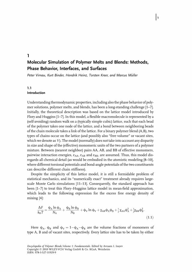
which become system size independent and cross at the critical point (Figure 1.1).M denotes the order parameter of the transition. For liquid–vapor phase coexistenceit is given by:

M � r�hri ð1:19Þ

In practice, we perform several simulations close to the critical point for differentsimulation box volumes and determine the coexistence chemical potential asindicated above. These simulations can be extrapolated to different temperaturesclose to Tc to obtain UK ðV ;TÞðK ¼ 2; 4Þ. The critical point is the intersection pointof the cumulants. The computation of cumulants is closely related to finite-sizeeffects [95–97] that haunted computer simulations in the early days but are nowunder firm control: In a macroscopic system the correlation length diverges at the

1.7 1.71 1.72 1.73 1.74temperature [ε/k]

1.2

1.4

1.6

U2,

U4

U2

U4

3d IsingL= 13.5 σ L= 11.3 σL= 9 σ L= 6.74 σ

Figure 1.1 Second- and fourth-ordercumulants for a LJ þ FENE pentamer incomparison to the corresponding values for the3d Ising distribution at criticality (horizontal

straight lines). Each line has been extractedfrom a single simulation by extrapolating thedata set to several temperatures. Adapted fromReference [47].


critical point. In a system of finite size, the correlation length can at most be equal tohalf of the linear dimension of the simulation box, which has to be considered in thevicinity of Tc. Definition (1.19) is sufficient formost purposes. Note, however, that anexact mapping of fluid criticality to Ising criticality has to consider field-mixingeffects [92] and M becomes a linear combination of density and energy. Owing tohigher order effects and corrections to scaling the values of U4 and U2 at theintersection points of the curves in Figure 1.1 deviate slightly from the asymptoticvalues obtained for the 3d Ising model (dotted horizontal lines). Note, however, thatthe intersections of bothU2 andU4 occur at about the same temperature, which canbe determined with good accuracy.

Away from the critical point, that is, at low temperatures, both phases are separatedby a free energy barrier that corresponds to a region of low probability. This barriercannot be overcome by thermal fluctuations. Several sophisticated schemes havebeen devised to address this issue. Multicanonical methods [98] modify theHamiltonian in order to sample a range of densities uniformly. To this end, a weightfunction w½n� is added to the original Hamiltonian. The simulated distributionPsim ðnÞ ¼ PðnÞ exp ð�w½n�Þ becomes flat for the choice of wðnÞ � ln PðnÞ. Unfor-tunately, PðnÞ is a priori unknown, but can be estimated by extrapolating an over-lapping data set [91]. A sequence of simulations and extrapolations typically startsclose to the critical point where barriers between both peaks are small and noweighting is required for the first run. The weight function wðnÞ can also be self-adjusted during simulation [99–102]. Note, that some of these schemes violatedetailed balance and bear the risk of systematic errors. However, they are well-suitedto generate an educated guess for the probability distribution, which can be used in aweighted simulation with fixed weights. A detailed discussion of methods toovercome free energy barriers can be found in Reference [103].

In the followingwe focus on a scheme that is based onumbrella sampling [104] andcircumvents most of these problems. In successive umbrella sampling [105] therelevant range of states is subdivided into small windows that are sampled consec-utively. This allows us to simulate without a weight function or to generate a weightfunction on the fly fromprevious windows bymeans of extrapolation. In the simplestimplementation, we start with an empty box and allow the system to change onlybetween 0 and 1 particle. A histogramHðnÞmonitors how often each state is visited(n denotes the number of particles in the simulation box). After a predeterminednumber of insertion/deletionMonteCarlomoves, the ratioH(1)/H(0) is determined,and we move the window to the right (to allow 1 and 2 particles). This procedure isrepeated until all relevant states have been sampled. Then, the (unnormalized)probability distribution can be estimated recursively:

PðnÞPð0Þ ¼

Hð1ÞHð0Þ �

Hð2ÞHð1Þ � � �

HðnÞHðn�1Þ ð1:20Þ

or:

lnPðnÞPð0Þ ¼ ln

Hð1ÞHð0Þ þ ln

Hð2ÞHð1Þ þ � � � þ ln

HðnÞHðn�1Þ ð1:21Þ


Logarithms are used to increase numerical accuracy as probabilities can becomevery low. The efficiency of the algorithm can be increased by combining the schemewith the multicanonical concept. In a weighted simulation we replace HðnÞ inEq. (1.20) by HðnÞ exp½�wðnÞ�. After P ðnÞ is determined according to Eq. (1.20),wðnÞ ¼ ln ½PðnÞ� is extrapolated to the next window and used as an educated guess forwðnþ 1Þ.

Once the probability distribution is determined, information about interfacialproperties can be extracted. Half way in between the gas and the liquid phase wetypically observe configurations in which half of the simulation box is filled withliquid and half of the box is filled with gas at coexistence density (Figure 1.2 inset). Asthe free energy of the coexisting phases is the same, the difference in free energy canbe attributed to the presence of the interface [106]:

c ¼ kBT2L2

lnPðnmaxÞPðnminÞ ð1:22Þ

The interface area is L2; the factor of 2 arises from periodic boundary conditions.P(nmax) is the average height of both peaks and P(nmin) theminimum in between. Forthese measurements an elongated box is preferred to ensure that the two interfacesdo not interact [107, 108].

Finally, we briefly mention an example that combines a coarse-grained modelingansatz with grand canonical simulations. In this particular case, hexadecane ismodeled as a chain of five coarse-grained Lennard-Jones beads [Eq. (1.9)] that areconnected by FENE [Eq. (1.10)] springs [48]. The solvent, carbon dioxide, is repre-sented by a simple Lennard-Jones bead that contains an additional r�10 term toaccount for the (spherically averaged) quadrupolar moment of CO2 [82, 111].Simulation parameters e, s, and q (for CO2) are derived by equating the criticaltemperature, the critical density, and the quadrupolarmoment (in the case of CO2) ofsimulation and experiment for the pure components. Mixture parameters eAB and

Figure 1.2 Free energy as a function of the number of LJ þ FENE pentamers (n) in the simulationbox (T ¼ 1:38 e=kB; V ¼ 9� 9� 18s3). Inset: typical configuration for n ¼ 100 pentamers. Withpermission from Reference [47].


sAB are given by the Lorentz–Berthelot combining rule (eAB ¼ jffiffiffiffiffiffiffiffiffiffieAeB

p, j ¼ 1,

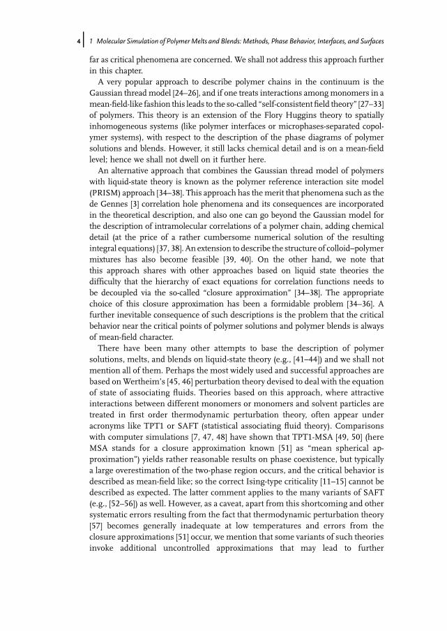
sA ¼ 0:5ðsA þ sBÞ). Figure 1.3 shows a projection of the phase diagram and thecritical line onto the pressure–temperature plane. Even though the model is verysimple and lacks atomistic details it can describe adequately the phase behavior of themixture without additional fitting parameters. If, however, the quadrupolar momentof CO2 is not taken into account, a modification of the Lorentz–Berthelot rule isrequired (j < 1). This emphasizes that atomistic detail is not always required todescribe the phase behavior correctly. However, it is advisable to include physicallyrelevant quantities like the quadrupolar moment of CO2.

1.3Wetting and Phase Diagrams in Confined Geometries

1.3.1Length and Energy Scales of Minimal, Coarse-Grained Models for Polymer–SolidContacts

While previous sections have focused on the bulk phase behavior and the propertiesof interfaces between coexisting bulk phases, the polymer material is often confinedin a container or a thin polymer film is supported by a substrate. This confinement

700 800600500400300200temperature T [K]

0

100

200

300

pres

sure

p [b

ar]

exp: lv coexist. exp 1: crit. lineexp 2: crit. linesim: lv coexist. ξ=1.000ξ=0.886q=0.387, ξ=1

critical point CO2 critical point C16H34

Figure 1.3 Projection of the global mixturephase diagram of a hexadecane–CO2 mixtureonto the pressure–temperature plane.Simulation results for the liquid–vaporcoexistence of the pure components are shownby circles. Thick lines mark two differentexperimental observations of the critical linefrom References [109, 110]. The thin dash-dotted lines indicate the experimental liquid–

vapor coexistence of the pure fluids. Crossesmark the critical mixture line obtained for a CO2

model that includes a spherically averagedquadrupolar moment, and no modification ofthe Lorentz–Berthelot mixing rule. Trianglesand squares denote the critical line for a CO2

model without quadrupolar moment with(triangles) and without modification (squares)of the Lorentz–Berthelot rule.


can give rise to wetting phenomena and these effects may profoundly alter the phasebehavior in confined geometry [112].

In the following, we assume that the confining walls of the container or the sup-porting substrate (e.g., awafer) are hard andnon-deformable, that is, the properties ofthe solid do not change as it is brought into contact with the polymermaterial. If onemeasures the density profile of the polymer material at the polymer–solid contact,one will typically observe a steep rise of the density from zero (in the solid, confiningwall) to the bulk density of the polymer material. The spatial extension of thispolymer–solid interface is only a few ångstr€om, that is, its width is dictated by the sizeof the atomistic constituents. On the other hand, in multicomponent polymermaterials (i.e., polymer blends or polymer–solvent mixtures) one component willenrich at the solid surface, and the width of these enrichment layers may extend faraway from the solid surface.

Two different enrichment phenomena can be distinguished [113]:

1) If the multicomponent material is completely miscible in the bulk, then acomponent will typically adsorb at the preferential, solid surface. This phenom-enon alters the composition profile near the polymer–solid contact on a lengthscale that is set by the molecular extension. The enrichment layers are muchlarger than the width of the polymer–solid interface but they cannot growmacroscopically large.

2) If the multicomponent material exhibits two coexisting phases in the bulk, thenone phase will be enriched at the polymer–solid contact and, provided that thesolid is sufficiently preferential, this wetting layer of the preferred phase willgrow macroscopically thick. One says that the preferred phase of the polymermaterial wets the solid [114].

In both situations the polymer–solid interface is much thinner than the width ofthe enrichment layer or the interphase. Since previous sections have dealt withphase coexistence in multicomponent polymer materials, we restrict ourselves tothe wetting phenomena (2) and refer the reader to References [115–117] forsimulation studies of adsorption phenomena within the framework of coarse-grained models.

The properties of the polymer–solid interface are most suitably investigated byatomistic modeling approaches. Atomistic modeling can address the complexinteractions between polymer and solid materials and study the subtle conforma-tional changes and structuring effects of the polymer liquid in the ultimate vicinity ofthe solid. However, atomistic approaches cannot address the length and time scalesrequired to build up and equilibrate wetting layers.

Systematic coarse-graining schemes have been applied to one-component poly-mer melts in contact with solid surfaces. In this framework, one starts with anatomistic modeling approach and systematically devises effective free energies ofinteraction between coarse-grained segments along the polymer. In this way,information on the atomistic scale may be transferred into coarse-grained models.An interesting example of this strategy is the investigation of polycarbonate at anickel surface where a strong, specific adsorption of the chain ends to the solid

1.3 Wetting and Phase Diagrams in Confined Geometries j15

surfaces has been revealed by atomistic modeling and this specific adsorption hasbeen incorporated in the coarse-grained model [118]. Without the underlyingatomistic modeling this specific interactions could have been easily overlooked.This example highlights the (rather special) case of a coupling between atomisticsurface properties and long-range conformational properties. Typically, however,the surface tension of a polymer melt exhibits only a weak dependence onmolecular weight.

If one uses a coarse-grained approach, one has to identify the relevant propertiesthat the description on the coarser scale has to capture. In the following, wespecifically consider wetting phenomena in a binary AB polymer blend that exhibitsliquid–liquid phase separation between an A-rich and a B-rich phase. The thermo-dynamics of the surface enrichment layers is dictated by the free energies of the solidin contact with the two coexisting phases, cAW and cBW, and their interfacial tension,cAB. If the solid surface, W, attracts the A-rich phase, then a domain of the A-richphase, which is embedded in the B-rich phase, will form a drop at the solid surface.The AB-interface at the boundary of the domain will make the contact angle,H, withthe solid wall, W. Young�s equation describes the balance of forces at the three-phasecontact line parallel to the solid surface and dictates [119]:

cWB�cWA ¼ cABcosH ð1:23Þ

Note that the surface tensions, cWB and cWA, are large. On the atomistic scale thereare strong forces and, consequently, the energy of a segment with the surface canexceed the thermal energy scale, kBT , by far. Moreover, the steep rise in density at thenarrow polymer–solid contact gives rise to important changes of the conformationalentropy (Lifshitz entropy [27]). In contrast, the interfacial free energy, cAB, is verysmall on the length scale of a coarse-grained segment. For a strongly segregated,symmetric binary polymer blend, one obtains [28]:

cAB ¼ kBTrb2

ffiffiffiffiffiffiffiffix=6

pð1:24Þ

where b denotes the statistical segment length, r the number density of coarse-grained segments, and x the Flory–Huggins parameter, which describes the repul-sion between segments of the different polymer species of the blend.

Typically, the Flory–Huggins parameter is very small, that is, of the order 1=N.Therefore, the left-hand side of Young�s equation, Eq. (1.23), consists of a cancellationof two large contributions. It is a formidable task to predict via atomisticmodeling thedifferenceDc ¼ cWB�cWA or theFlory–Huggins parameter,xwith an accuracy of theorder kBT=N per segment.

The behavior of polymer solutions, which exhibit phase coexistence between apolymer-rich liquid (L) and a polymer-poor vapor (V), is qualitatively similar. Only theseparation of energy scales between the surface tensions of the polymer and vapor incontact with the solid and the liquid–vapor interfacial tension is less pronouncedbecause the liquid–vapor interface also is narrow and the cohesive van der Waalsinteractions inside the liquid are strong.


The idea of aminimal coarse-grainedmodel for polymer–solid contacts consists innot describing the structural details of the polymer–solid contact on the length scaleof Ångstr€oms because this length scale is not resolved. Instead, the aim is to tailor theinteractions at the surface in order to match the difference in surface tension, Dc, ofthe coarse-grained model to the experimental data. In this way, the macroscopicinterfacial thermodynamics is parameterized.

Another important ingredient, which determines the wetting behavior, is theinteraction between the outer, liquid–vapor interface of thewetting layer and the solidsurface. This interaction (per unit area) is denoted as the interface potential [114] andit dictates, inter alia, the order of the wetting transition and the way, in which thethickness of the wetting layer grows as one approaches the bulk phase coexistence byvarying the pressure.

Generally, the interface potential consists of a short-ranged and long-rangedcontribution. The short-ranged potential stems from the distortion of the densityprofile at the interface. It decays exponentially as the thickness of the wetting layerincreases and its length scale is set by the decay length in the wings of the interfacialprofile, that is, the bulk correlation length, j � Re.

The long-ranged part of the interface potential arises from the integratedvan derWaals interactions inside the polymermaterial and between the solid surfaceand the polymer. This long-ranged interaction can be described by an externalpotential, which decays like [32]:

V lrwallðzÞ ¼ |{z}

DA6pr

ewall

� 1z3

ð1:25Þ

The strength, ewall, is parameterized by the Hamaker constant, A, which isproportional to the energy parameter, e, of the Lennard-Jones potential. Typically,in a coarse-grained model, the Lennard-Jones interactions are cut-off at a finitedistance, cf. Eq. (1.9). Therefore, the strength, DA, is the difference between theHamaker constant of the interactions inside the polymer liquid and that betweenpolymer and solid.

To describe the thermodynamics and structure of wetting layers at a polymer–solidcontact within the framework of aminimal, coarse-grainedmodel, one has to identifythe bulk properties, Flory–Huggins parameter, xN, the mean-squared end-to-enddistance, Re, and the molecular density, r=N. Re characterizes the gross featuresof the molecular shape on large length scales, and xN and r=N can be identified,for example, by matching the critical point of the blend or solution to experimentaldata. The structure and thermodynamics of the polymer–solid contact requires(at least) two additional, coarse-grained parameters – the difference in the surfacetension, Dc, between the two coexisting phases and the strength of the long-rangedinteractions. The former can be identified by the macroscopic contact angle that adrop of the A-rich phase or polymer-rich phase embedded in a B-richmatrix or vapormakes with the solid surface. The latter can be estimated from experimental data onthe Hamaker constants.


1.3.2Measuring the Surface Free Energy Difference, Dc, by Computer Simulation

Here we discuss how to determine the additional coarse-grained parameters thatcharacterize the coarse-grained model of the polymer–solid contact using theexample of a one-component polymer material, which exhibits liquid–vapor phasecoexistence. Knowing the bulk phase behavior and the interfacial tension betweenthe coexisting phases, one could determine the difference, Dc, by measuring thecontact angle of a cap-shaped drop on the solid surface. This procedure mimics theexperimental measurement but, unfortunately, the small droplet sizes accessible insimulations gives rise to significant finite-size effects:

1) If a drop is formed on the surface, the chemical potential of the system willbe shifted away from the bulk coexistence value (Kelvin equation). Drops of agiven size are only stable for a certain range of system sizes. If the system size istoo large, the system will rather dissolve the excess material homogeneouslyin the volume than pay the free energy cost of the liquid–vapor interface [121].This is the analog of the droplet condensation–evaporation transition in thebulk [122].

2) The contact angle of a small droplet may significantly be affected by the effectsof the line tension that describes the free energy costs of the three-phasecontact between liquid, vapor, and solid. This effect can be greatly reduced byconsidering cylindrical droplets that span the simulation box in one directionvia the periodic boundary condition. In this case, the length of the three-phasecontact line is twice the width of the system independent from the droplet sizeor contact angle [123].

3) The contact angle is defined by the asymptotic behavior of the liquid–vaporinterface approaching the surface. At short distances from the surface, theinteraction between the interface and the surface – the interface potential –distorts the interface away from its asymptotics and, thus, it may be verydifficult to identify the asymptotic behavior from simulation data of smalldrops [31].

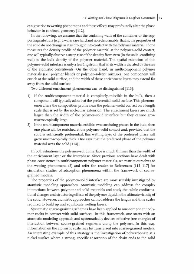
These difficulties will be avoided if one directly computes the surface freeenergy difference. To measure surface free energies, we apply the same grand-canonical Monte Carlo technique that we used for the bulk thermodynamics(Section 1.2.3), now in the presence of two surfaces [120, 124]. We fix the chemicalpotential to its coexistence value and, using the re-weighting method, we canmake the simulation sample all densities between the vapor phase (V) and theliquid phase (L) in contact with the surface. Again the logarithm of the probabilitydistribution, P, yields the free energy as a function of the density. Figure 1.4displays the results for the Lennard-Jones bead-spring model with N ¼ 10effective segments at temperature kBT=e ¼ 1:68. The free energy exhibits twominima, corresponding to configurations where either a vapor (low density) or aliquid (high density) phase is in contact with the surface. The ratio of theprobability for finding the system in one of these phases yields the difference


in the surface free energies:

Dc � cVW�cLW ¼ kBT2L2

lnPðwLÞPðwVÞ

�ð1:26Þ

where 2L2 denotes the area of the two surfaces. Note that the bulk does not yieldany contribution to the difference because, at coexistence, the grand-canonicalfree energies (i.e., pressure) of the two coexisting phases – liquid and vapor –are identical.

At intermediate densities the typical conformations consist of a liquid slab at eachwall. If the system size is sufficiently large the distance between the liquid–vaporinterfaces and the wall and their mutual distance become large. In this limit theinterfaces neither interact with the walls nor with each other, and we expect only aweak dependence of the free energy on the density, that is, a plateau in the probabilitydistribution, P, at intermediate values of the average density. The liquid will wet thesurface if the difference in surface tensions equals the interfacial tension,Dc ¼ cLV.In a sufficiently large system, the wetting transition corresponds to the point wherethe plateau value of P equals PðwVÞ.

For the system size studied in Figure 1.4, we do not observe a plateau, that is,once the interfaces have reached a distance from the wall, which is large enough

0.00 0.20 0.40 0.60

φσ3

0.00

0.05

0.10

0.15

∆F/2

L2 kBT

εw=2.9εw=3.15εw=3.2εw=3.3εw=3.4

γVW−γLW

γLV

Figure 1.4 Illustration of the simulationtechnique for a one-component, bead-springmodel at temperature kBT=e ¼ 1:68 and mcoex.A cuboidal system geometry 13:8s� 13:8s�27:6s with periodic boundary conditions inthe two short directions and two confiningsurfaces in the long direction is used. The curvesare shifted such that the free energy of the liquid

phase vanishes. The horizontal arrow on the leftmarks the value of the interfacial tension cLV,while the vertical arrow marks the difference inthe surface tension between the vapor/wall andliquid/wall for ew ¼ 3:15. Typical systemconfigurations are sketched schematically.Adapted from Reference [120].


for the interface potential between the interface and the surface to decay, theyalready begin to interact mutually. This indicates that our simulation cell is toosmall to accommodate two non-interacting solid–liquid and liquid–vapor interfaces.Nevertheless, we can reliably determine cVW�cLW. In these limiting states, thecontainer is either completely filled with vapor or liquid, and there are no liquid–vapor interfaces present. The perturbation of the density profile in the liquid extendsonly over a few segmental diameters, s, which is much smaller than the extension ofthe simulation cell.

To parameterize the coarse-grainedmodel to a specific physical realization, onehasto tune the interactions, Vwall, between solid and polymer to reproduce the exper-imental value of the surface free energy difference, Dc. Once Dc has been obtainedvia the method described above for a particular strength, ewall, of Vwall, the depen-dence on the attractive strength of the wall can be obtained via thermodynamicintegration [120, 124]:

VðewallÞ ¼ VðeoÞþðewalleo

dew0hEwallðew0 Þi

ew0ð1:27Þ

whereV is the grand canonical potential and Ewall ¼ L2ÐdzwðzÞVwallðzÞ denotes the

interaction energy associated with the monomer–wall interaction potential. Like anythermodynamic integration, this procedure can be efficiently carried out in theframework of an expanded ensemble.

1.3.3Application to Polymer–Solvent Mixtures

To illustrate these techniques, we consider the coarse-grained model for hexadecaneand carbon dioxide, which we have discussed in Section 1.2. The correction of theLorentz–Berthelot rule is set to j ¼ 0:9 and the temperature is fixed at kBT=e ¼ 0:92.(In this case carbon dioxide was modeled as a simple Lennard-Jones bead withoutquadrupolar moment.) The short- and long-ranged interactions at the polymer–solidcontact are described by a 9-3-potential of the form:

Vwall ¼ eWSðPÞsSðPÞDz

� �9� sSðPÞ

Dz

� �3 �

ð1:28Þ

where eWS and eWP, denote the strength of the surface interaction acting on solventand polymer, respectively.

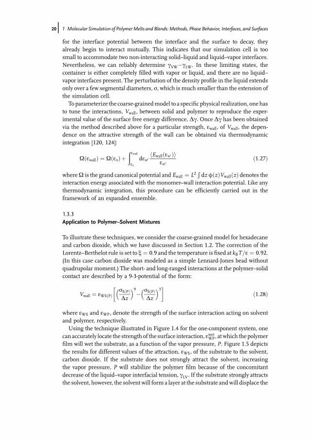
Using the technique illustrated in Figure 1.4 for the one-component system, onecan accurately locate the strength of the surface interaction, ewetWP, atwhich thepolymerfilm will wet the substrate, as a function of the vapor pressure, P. Figure 1.5 depictsthe results for different values of the attraction, eWS, of the substrate to the solvent,carbon dioxide. If the substrate does not strongly attract the solvent, increasingthe vapor pressure, P will stabilize the polymer film because of the concomitantdecrease of the liquid–vapor interfacial tension, cLV. If the substrate strongly attractsthe solvent, however, the solvent will forma layer at the substrate andwill displace the


polymer. The excess of solvent at the surface may lead to dewetting of the polymerfilm upon increasing the pressure. This effect has also been corroborated by self-consistent field calculations [125, 126].

1.4Molecular Dynamics Method

1.4.1Basic Molecular Dynamics

Molecular dynamics [127] (MD) is a numerical technique to approximate the staticand dynamic properties of classical many-body systems. MD techniques are com-monly employed alongside Monte Carlo techniques because dense packing reducesthe acceptance probability of translation and chain rotationmoves to very low values,particularly when using all-atom models.

The key idea is simple: ifUðfr igÞ is the total potential acting on particle iwithmassmi and position r iðtÞ at time t, then Newton�s equations of motion (EOM):

miq2

qt2r iðtÞ ¼ �riUð r if gÞ ð1:29Þ

are solved iteratively. Themain justification of theMDmethod is based on the ergodichypothesis that time averages are equal to statistical ensemble averages. However,MD simulations generate cumulative errors that cannot be suppressed entirely, butare minimized using adequate integration schemes. Various algorithms have beensuggested to solve Eq. (1.29).

0.00 0.05 0.10 0.15 0.20

Pσ3/kBT

3.0

3.5

4.0

4.5

5.0

5.5

6.0

ε WP

wet

εWS=0εWS=1.5εWS=10

kBT/ε = 0.92

Figure 1.5 Dependence of the wetting transition ewetWP on pressure,P, estimated by grand-canonicalMonte-Carlo simulations of a polymer–solvent mixture. Adapted from Reference [125].

1.4 Molecular Dynamics Method j21

TheVerlet algorithmuses the Taylor expansions of the position vectors in differenttime directions. With Dt the �time-step� of the simulation, adding the expansionsfor r iðtþDtÞ and r iðt�DtÞ leads to:

r iðtþDtÞ ¼ 2r iðtÞ�r iðt�DtÞþ aðtÞDt2 þOðDt4Þþ � � � ð1:30Þ

where aiðtÞ ¼ �riUðfr igÞ=mi denotes the acceleration. When terms larger thanOðDt3Þ are neglected one obtains positions that are correct to OðDt4Þ, whereasvelocities are correct to order OðDt2Þ.

A commonly applied modification is the velocity Verlet algorithm. It explicitlyincorporates the particle�s velocity, vi, such that:

r iðtþDtÞ ¼ r iðtÞþ viðtÞDtþ aiDt2

2

viðtþDtÞ ¼ viðtÞþ aiðtÞþ aiðtþDtÞ2

Dtð1:31Þ

This approach produces errors that are of the same order as the Verlet algorithm.Its advantage lies in symmetric coordinates for �past� and �future� and conservationof the phase-space volume, that is, the velocity Verlet algorithm is consistent withLiouville�s theorem. Although energy is not conserved perfectly on short time scales,there are no energy drifts for large times. The stability of themethod canbe increased,for example, using �Beeman�s algorithm� [128] or the �leap-frog� [129] method,which calculate the velocities more accurately.

In predictor–corrector algorithms time derivatives of the position vectors at time tare used to predict the positions and their derivatives at time tþDt. The predictedvariables then are corrected according to the difference from those at time t, where aset of �Gear constants� are used. The latter are chosen to balance accuracy andstability, that is, short- and long-time conservation of energy. Optimized valuesdepend on the order of the Taylor expansion (�order of the algorithm�).

Predictor–corrector algorithms are only time reversible for Dt! 0 and thereforeviolate Liouville�s theorem.However, in the canonical ensemble they can be tuned tobe more accurate than the Verlet integration.

The main computational effort in MD simulations is to evaluate the interatomicforces. For pair-wise additive and short-range potentials geometrical compositionalgorithms have been proposed to optimize the force calculation. Mostly appliedare the �cell linked-lists� or the �Verlet list� algorithm. Examples for efficientmethods to compute forces from long-range potentials are �Ewald summation� [130],�particle-mesh Ewald� [131], �particle-particle-particle-mesh� [132], and �generalizedBorn� [133] algorithms.

The MD method has become a powerful tool to simulate even millions of par-ticles and arbitrarily complex molecules in confined systems or in the bulk usingperiodic boundary conditions. Modifications of the original approach allow for MDsimulations at constant pressure, chemical potential, or temperature. �Ab initio�MDsimulations [134], using first-principles to evaluate interatomic forces for quantumelectronic systems, have led to remarkable accomplishments in simulating theproperties of real materials.


1.4.2Non-equilibrium Molecular Dynamics Simulations of Coarse-GrainedPolymer Systems

Computational studies of polymeric liquids under non-equilibrium conditions havebeen performed intensively in recent decades [135–152]. This is not only related tothe advancing computational resources that have made such studies possible, butmainly to the distinct advantages of numerical investigations. While experimentsusually only provide information on macroscopic properties, non-equilibriummolecular dynamics (NEMD) simulations allow one to explore structural features,which can be related to the phenomenological coefficients that describe the trans-port of mass, momentum, and energy. NEMD simulations have reproduced suc-cessfully many qualitative features of polymer solutions under stationary (steady)shear, such as �shear thinning� (decreasing viscosity with shear rate), �shearalignment� or effects on the normal stress [137, 139–142, 144, 145, 147, 149, 150].Meanwhile, many numerical studies have been performed even for nonstationaryflow fields [140, 145, 146, 150]. However, a reliable characterization of systems outof equilibrium requires careful numerical approaches, where special attention mustbe paid to coarse-graining, boundary conditions, and thermostat issues. In thissectionwe discuss some of these technical aspects inmesoscopicNEMDsimulationsfor coarse-grained polymer systems.

A presentation that covers the entire field of NEMD simulation techniques wouldgreatly extend the length of this section. Here, we focus mainly on the case ofconfined polymer systems, where shear deformation is induced by displacement ofthe confining boundaries. The simulation of bulk systems usually invokes othertechniques than discussed here, which are often better suited to reveal homogeneousfluid dynamics. For instance, homogeneous flow fields can be generated by deter-ministic (e.g., SLLOD [135, 136, 138, 148, 152]) EOM, which have been shown toreveal rather accurate transport properties for atomic liquids [138].However, complexfluids, such as polymer solutions or melts, tend to �align� under strong shear-deformation due to hydrodynamic instabilities. Homogeneousmethods that enforcea linear shear profile therefore have to be applied with care. Simulation methods foratomistic and molecular fluids in homogeneous flow fields have been reviewed indetail [152].

The rigorous solution of the time-dependent, quantum-mechanical, many-bodyproblem is numerically unfeasible. The problem thus must be reduced to classicalmechanics and coarse-grainedmodels have to be introduced. In particular forNEMDsimulations, the modeling of solvent effects can be crucial and the complexity of theproblem is highly dependent on whether the external stimuli are strong or weak andwhether they are constant in time or nonstationary.

Whenhydrodynamic effects are not expected to be important, it is often convenientto simulate without explicit solvent molecules. This approach can still be justifiedeven when hydrodynamic flow becomes relevant, but solvent-related degrees offreedom have to be incorporated on a certain coarse-grained level. To reproducehydrodynamic effects in the continuum limit, mesoscale hydrodynamic techniques


have been developed that conserve local mass and momentum. Such methods, forexample, dissipative particle dynamics [143, 147, 149–151, 153–172], stochasticrotational dynamics [173–181], and the lattice Boltzmann method [182–185], canreproduce hydrodynamic behavior described by the Navier–Stokes equation on therelevant (large) length scales. In these approaches, monomers interact via conser-vative and thermal forces, where the latter are introduced via a thermostat.

Upon using a thermostat, one assumes that heat transport within the system occursinstantaneously. This is not strictly correct but often it is convenient to simulate atconstant temperature. Fluctuation relations are derived more straightforwardly thanfor the micro-canonical ensemble and the thermostat helps to stabilize particletrajectories, allowing theuseof larger timesteps. InNEMDsimulations, the thermostatis of great importance, as it is used to remove the viscous heat due to the entropyproduction fromexternal stimuli.However, it is a non-trivial challenge inmanyNEMDsimulations of complex fluids to maintain the temperature and simultaneously avoidan undesired influence of the thermostat on transport properties. For simulations farbeyond static equilibrium, the specific choice of the thermostat and its parameters areoften crucial. One example, where complications may arise easily, is the sheardeformation of confined polymer systems, which is often simulated at shear ratesmuch larger than typical experimental values (see References [142–144]) in order toobtain statistically meaningful results.

Owing to its simplicity, the Langevin (LGV) thermostat is one of the most appliedmethods to perform simulations in the canonical ensemble. In this approach, thesimulated particles are coupled to an external heat bath at constant temperature. Thedissipative force acting on particle i is proportional to its velocity:

F di ¼ �miCvi ð1:32Þ

where C is a friction constant. The random force follows from the fluctuation–dissipation theorem, which defines the temperature of the simulation. The LGVthermostat acts on a local scale. Particles that are too fast are damped by the viscousbackground, whereas the stochastic heat bath increases the velocity of particles thatare too slow. As this method stabilizes the trajectories of monomers very efficiently,the LGV thermostat has been applied for many previous studies [137, 139, 141, 142,144, 145, 150] of polymeric systems, both in static equilibrium and in NEMDsimulations. However, the LGV thermostat does not conserve momentum andscreens hydrodynamic interactions beyond a length [170, 186]:

k ¼ffiffiffiffiffiffig

rC

rð1:33Þ

where g and r are viscosity and density, respectively.Galilean invariance is lost due to the coupling ofmonomers to the heat bath, which

mimics a solvent that rests in the laboratory frame. Therefore, themethod belongs tothe class of �profile-biased� thermostats [138]. This can be demonstrated easily: Let usconsider a film of linear polymers confined by two adsorbing substrates. Shear isapplied by moving the upper substrate with a constant velocity, w, while the lower


substrate remains at rest. For a large film thickness, L, the density inhomogeneitiesclose to the substrates are negligible. With gbulk as the bulk viscosity, the Navier–Stokes equation reads [145]:

gbulkDvðzÞ ¼ CrvðzÞ ð1:34Þ

where zdenotes the gradient direction, vðzÞ is the velocity profile, andr themonomermass density.

Solving Eq. (1.34) with stick boundary conditions at the lower substrate, vxð0Þ ¼ 0(x the shear direction), and assuming vxðLÞ w for the upper, leads to [145, 170]:

vxðzÞvxðLÞ ¼

sinhffiffiffiffiffiffiffiffiffiffiffiffiffiffiffiffiffiffiCr=gbulk

pz

� sinh

ffiffiffiffiffiffiffiffiffiffiffiffiffiffiffiffiffiffiCr=gbulk

pL

� ð1:35Þ

for the monomer velocity profile. The shear stress, sxz, can be obtained fromintegrating over the dissipated force [right-hand side of Eq. (1.34)], and forL ffiffiffiffiffiffiffiffiffiffiffiffiffiffiffiffiffiffi

gbulk=Crp

one finds sxz � C1=2. Simulations [145] confirmed this scalingbehavior and revealed velocity profiles as given in Eq. (1.35). This outcomeobviously is determined by the thermostat, as Eq. (1.34) describes the couplingof monomers to a solvent that remains at rest in the laboratory frame, independentof shear rate [145, 170].

To circumvent a biasing of flow profiles in shear simulations, the LGV thermostatis often applied anisotropically [137, 139, 141, 145, 150]. For instance, the thermostatforce may be applied only in gradient and vortex directions, but �deactivated� alongthe direction of shear. Recent results [150] indicate that, under certain circumstances,a good agreement between this implementation and a method that intrinsicallyprovides Galilean invariance can be achieved (see below). However, the couplingbetween the shear and gradient directions in complex fluids demands specialattention whenever this feature becomes relevant for the transport properties ofthe confined fluid.

The most straightforward modification of the LGV thermostat is to relate thethermostat forces to the relative velocity of interacting particle pairs. Such anapproach is based on the dissipative particle dynamics (DPD) method. Originally,DPD was proposed in conjunction with �soft� interaction potentials, which wouldrepresent clusters of atoms, increasing the stability of particle trajectories andallowing the use of larger MD time steps than for �hard� potentials. It has beenapplied to various problems, for example, phase separation [161, 164, 166], theflow around complex objects [153], and colloidal [154, 162] and polymeric [143, 147,149–151, 157, 158, 167, 170] systems.

When DPD is applied as a thermostat, dissipative and random forces are addedto the total conservative force in a pair-wise form. The sum of thermostat forcesacting on a particle pair vanishes such that the microscopic dynamics fulfillsNewton�s third law. This method provides momentum conservation and Galileaninvariance.


At large densities, the DPD thermostat reveals the coupling between the shear andgradient directions and hence is well suited for shear simulations of polymer melts.However, it is important to note that DPD cannot describe hydrodynamic behavior atarbitrary densities when solvent effects are not otherwise incorporated. This affectsthe applicability of the DPD thermostat already in static equilibrium, where it fails toreproduce Zimm dynamics [189] due to the missing long-range interaction betweenmonomers transmitted by the solvent. To account for hydrodynamic correlations inthe dilute regime, solvent effects have to be included on whatever coarse-grainedlevel [143, 147, 157, 165, 167–169, 171], for example, by introducing explicit solventmonomers.

Modified versions of DPD are frequently proposed and the advantages and short-comings of such modifications are a current issue of research [150, 172, 187].DPD can be transformed into �smooth-particle hydrodynamics� [188], where theNavier–Stokes equation is solved in a Lagrangian form, or by the application of asplitting algorithm [169] into an Andersen�s-thermostat version [165]. The DPDmethod can also be applied in the micro-canonical ensemble [159, 160, 163]. Anextension of DPD has been introduced recently to allow for damping along theparallel and perpendicular components of the relative particle velocities indepen-dently [187]. This enables one to tune the transport properties of coarse-grainedliquids to bettermatch atomisticNEMDsimulations, whenever the latter are feasible.However, the new approach does not conserve local angular momentum and henceshould be used with care.

LGV and DPD thermostat have been compared recently [150] for NEMD simula-tions of polymer brushes. Apolymer brush formswhen linear polymers are adsorbedon substrates with one chain end, such that the steric repulsions betweenmonomersforce the chains to stretch away perpendicularly from the substrate. Systems of twopolymer-brush bearing surfaces in contact can sustain large normal loads, simul-taneously revealing small friction forces under shear deformation due to shearinduced chain inclination. Polymer brushes therefore are very important lubricantsand hence are the subject of many NEMD studies [137, 139–142, 144, 145, 147, 151].

For steady-state shear deformation similar transport properties are found at largeand intermediate monomer densities, but systematic differences between the twomethods arise at small densities. DPD and LGV thermostat also reveal somewhatdifferent results for nonstationary flows [150].

NEMD simulations of polymer brushes at constant shear motion have alsobeen performed with explicit solvent molecules, which are typically introduced as�single monomers.� Both the LGV thermostat [139] and DPD [143, 147] exhibitsignificantly enhanced lubrication properties as compared to simulations of �dry�brushes, revealing the importance of solvent-induced effects on the macroscopictransport coefficients.

Complex polymer systems, such as polymermelts [149, 150] or star polymers [190]embedded between two polymer brushes, have been the subject of recent investiga-tions. Simulations of these systems under nonstationary stimuli are extremely rare.

Alternative approaches to account for hydrodynamic interactions are based onso-called �hybrid� methods, where the polymers are coupled to a dynamical


background. The latter can be introduced either by collisions of ideal-gas particles orby a lattice-based solution of the Boltzmann equation [184], known from the kinetictheory of gases.

The first technique is known as the stochastic rotational dynamics (SRD) methodor multiparticle collision dynamics, which is a particle-based algorithm suited toaccount for hydrodynamic interactions on themesoscale. The coarse-grained solventis described as ideal-gas particles that propagate via streaming and collision steps,which are constructed such that the dynamics conserves mass, momentum, andenergy.

In the streaming step, the solvent particle trajectories are ballistic. Collisions areintroduced by sorting the particles into cubic lattice cells and performing a stochasticrotation of the relative velocities in each cell. In contrast toDPD, the SRDmethod actson all particles within the same collision cell.

In SRD, the environment of a particle depends on the superimposed velocity field.This breaks Galilean invariance, because the particles that participate in a collisiondiffer betweenmoving and resting frame. However, when the mean free path lengthof particles is large compared to the mesh size of the lattice, colliding particles arrivefrom different cells and are therefore uncorrelated. This reflects the conditions of�molecular chaos,� where Galilean invariance is negligible. It has been shown [175]that Galilean invariance can be restored by a randomization of the collision envi-ronment, for example, by random shifts of the cells before each collision step.

To simulate polymer solutions, themonomers have to be coupled to the SRD fluid.Different strategies to achieve this aim have been proposed [173, 174, 176–179, 181].Typically, the EOM of the polymers themselves are integrated with the standard MDmethod. The monomers are included into the collision step, thereby exchangingmomentum with the SRD fluid. This is carried out under conservation of the totalmomentum. Often it is sufficient to treat the monomers as hydrodynamic pointsources and to neglect the excluded volume interaction between solvent and mono-mers [173]. This method reproduces hydrodynamic behavior on large length scalesand therefore reveals Zimm dynamics for dilute linear polymers in static equilib-rium [173, 176, 177].

SRD appears to be a very promising (rather new) approach for future NEMDsimulations, as it is a very efficient mesoscale technique. It reflects the characteristicshear deformation of solute macromolecules, for example, for shear flows of starpolymers [180] or DNA molecules [181].

Hydrodynamic flow also can be incorporated via a discretized version of theBoltzmann equation. This approach is known as the lattice Boltzmann (LB) method.The idea is to solve the linearized Boltzmann equation on an underlying lattice topropagate molecular populations (�fictitious� solvent particles), which define thedensity and velocity on each lattice site. Similar to SRD, the monomers are treatedas hydrodynamic point sources in the continuous space. The flow velocity atthe monomer positions follows from a linear interpolation between neighboringlattice sites.

Coupling a stochastic version of LB with standard MD has allowed the reproduc-tion of Zimm dynamics for dilute polymers in static equilibrium [183]. It has been


applied recently to study polymer migration in confined geometries for pressuredrivenflows [191]. LB also can be used in somewhat different �hybrid�methods [182],where the �point-particle� assumption for the solute is no longer valid, for example, incolloidal systems [185].

The applicability of thermostat implementations and mesoscale hydrodynamictechniques depend strongly on the specific system under consideration and generalrecommendations in favor of one method cannot be made. However, some guide-lines shall be given:

. The LGV thermostat can be ruled out, even in its �profile-unbiased� version,whenever momentum transport is relevant, either in the form of hydrodynamicinteractions or, for instance, due to a coupling between the shear and gradientdirections.However, the LGV thermostat can be a powerful tool, as it stabilizes theparticle trajectories very efficiently and allows the study of systems far fromequilibrium. Excellent examples are investigations of polymer brushes at suffi-ciently large density, where situations far beyond linear response [137, 139, 141,142, 144, 145, 150] and nonstationary shear deformation [144, 145, 150] could bestudied.

. The DPD thermostat is the most straightforward and natural way to introduceGalilean invariance and momentum conservation. Whenever feasible, NEMDsimulations with DPD and explicit solvent molecules would yield reasonablemesoscale hydrodynamics. Simulations far beyond static equilibrium [143, 147,149–151] and nonstationary flows [150] have been performed. However, the levelof coarse-graining for the explicit solvent still is a relevant issue.

. The usage of monomers as hydrodynamic point sources coupled to a SRD or LBfluid invokes problems for some systems in NEMD simulations. For instance,shear induced instabilities related to compositional fluctuations at polymer–liquid interfaces cannot be described properly when excluded volume effectsare neglected. For nonstationary flow fields, a problem arises matching the timescales of polymer systemandbackgroundfluid.When adjusted incorrectly, effectsstemming from the finite solvent inertia may not be covered.

1.5Atomistic Simulation of Polymer Melts and Blends Using Molecular DynamicsTechniques

1.5.1Polymer Melts

Molecular dynamics simulations of polymermelts and blends in full atomistic detailare computationally demanding and a relatively recent approach to complementexperimental observations and advance polymer theory [192–201]. The numericalsimulation of Newton�s equation of motion with suitable interatomic potentials(force fields) for polymers and other common constituents [202, 203] contributes to


understanding of the structural, dynamic, thermal, and mechanical properties ofpolymer melts. First attempts employed rotational isomeric state models to generatean initial structure and energy minimization (a predecessor method to MD tominimize atomic overlaps), combined with �blowing up� interatomic potentials, toobtain independent static equilibrium models of polymer melts [192]. The systemsize has since increased from the simulation of a single atactic polypropylene chain ina box of 1.8 nm3 volume with a few independent configurations to complex polymersystems of 10 nm3 volume over periods of nanoseconds (millions of time steps offemtoseconds) using desktop computers and over periods of microseconds (billionsof time steps of femtoseconds) using supercomputers. The exponentially increasingamount of computational resources opens up new avenues to obtain insight into thedynamics of molten polymers.

In polyisoprene melts, the local polymer dynamics were shown to be independentof initial configurations [193]. Ratios of correlation times for different C–Hvectors inthe chain backbonematchNMRdata very well, while absolute values weremore thantwice as long. The spatial extent of cooperativemotion accompanying conformationaltransitions was found to be about 1–2 repeat units. Diffusion coefficients, frictioncoefficients, and zero-shear viscosities in models of linear polyethylene melts werecomputed in very good agreement with experiment [194]. Systems of several chainsof length C24 to C156 were first equilibrated using an efficient end-bridging MonteCarlo algorithm, and then subjected to MD simulation in the NVE and NVTensembles up to 12 ns. The resulting series of melt properties as a function of chainlength significantly expanded the understanding of polymermelts, including radii ofgyration and relaxation times. Most importantly, the friction coefficient j was foundto be constant above a chain length of C60, which is consistent with the Rouse modelfor an unentangled polymer melt (Figure 1.6).

Figure 1.6 Friction coefficient j versus chain lengthN of polyethylene, as obtained from the Rouserelation between j and diffusion coefficient D (jD, full symbols) and from the Rouse relationbetween j and the longest relaxation time t1 (jt, open symbols). After Reference [194].

1.5 Atomistic Simulation of Polymer Melts and Blends Using Molecular Dynamics Techniques j29

Molecular dynamicsmethodshave been further applied in industrial contexts [195]to gain qualitative insight into viscoelastic properties of polydisperse polymer melts,interface tensions between polymer melts, and the Izod impact strength. Nanopar-ticles of up to 16 nm diameter composed of chains of length C50 to C200 of variouspolymers (PE, PEP, aPP, PIB) were simulated by large-scale parallel MD to estimateglass transition and melting temperatures [196]. According to experiment, thethermal expansion coefficient and the heat capacity increase at the glass transitiontemperature; both increases were also observed in MD simulation at, however, twodistinct temperatures of 50 K below and 50K above the experimental glass transition.Nevertheless, a qualitative relation between increasing transition temperature andincreasing size of the polymer particles has been found. Results obtained so far havebeen insufficient to demonstrate conclusively the ability to simulate glass transitionsreliably and routinely, owing to the long time scales of the transitions and limitationsin accuracy of the atomistic models [197, 198]. Several chains of atactic polystyrene ofcomposition C400H402 were simulated to investigate the surface structure of thinfilms [199]. An end-bridgingMonte Carlo algorithmwas first invoked using a coarse-grained model for equilibration of the melt, followed by mapping onto the fullatomistic detail, and molecular dynamics simulation. A preferred orientation of thephenyl rings normal to the surface was found and a surface energy 38mJm�2 wascomputed in agreement with experiment. Moreover, dielectric properties of poly(butadiene) [200], glass transitions of various polymers [198], and force field para-meters for silamethylene polymers [201] were investigated.

1.5.2Polymer Blends

The simulation of polymer blends includes mixtures of polymers in the molten andsolid states [204–218]. We can distinguish miscible, partially miscible, and immis-cible blends as well as mixtures of very specifically interacting biopolymers. Forexample, direct contacts between residues in a protein (homeodomain of Antenna-pedia) and DNA bases, as well as the role of water molecules at the interface, havebeen analyzed during a 2 ns trajectory [204]. Dynamical observations by NMRspectroscopy were consistent with specific interactions derived from the simulation,and the critical role of the Gln-50 residue (pink) for protein–DNA binding, aspreviously known through genetic and biochemical analysis, could be linked to theinteraction with four base pairs and bases in both DNA strands (Figure 1.7). Thesimulation of similar specific protein–protein interactions [206] and protein–polymer interactions [213] is an interesting extension of the simulation of homo-polymers and block-copolymers.

After an efficient initial Monte Carlo equilibration with chain scission and fusionmoves, the diffusion of binary liquid blends of n-alkanes and polymers wasinvestigated for chain lengths of C5/C78, C10/C78, and C12/C60 using moleculardynamics simulation [207].Diffusion coefficients of both components increasedwithincreasing weight fraction of the short chain component, which was attributed to theincrease in free volume contributed by these solvent-like chains. Results were found


to be in good agreement with free volume theory for low andmedium fractions of theshort alkane, with Rouse theory for all volume fractions, and with measurements ofdiffusion constants for the C12/C60 system across the range of volume fractions andtemperatures.

More recently, glass transition temperatures were computed in semi-quantitativeagreement with experiment for a cationic polymethacrylate blended with triethylcitrate plasticizer as a function of plasticizer weight content using medium sizesimulation boxes (3.4 nm3) in the NPT ensemble (Figure 1.8) [212]. Results ofsimilar quality were also obtained for hydroxyl-terminated poly(butadiene) andpoly(glycidyl azide) with various amounts of plasticizers [218]. The findings illustratethe current ability and limitation of all-atom simulations to characterize the phasebehavior of polymers and blends as a function of chemistry. The reliability mightbe further improved through more accurate force fields, particularly with a focus onthe precisemodeling of polarity [219] and torsion barriers. In addition, stress tensorsat interfaces and in arbitrarily shaped volumes within the system can be computed todescribe the detailed dynamicmechanical behavior, including additive contributionsfrom bonded, Coulomb, and van der Waals interactions to the total stress [220].Notably, however, the quantitative prediction of glass transition temperatures meetsthe principal problem that the structural relaxation time of the polymer melt slowsdown dramatically in the temperature region slightly above the glass transition,where it reaches typically about 1 s. Molecular dynamics studies can equilibrateatomistic models of polymer melts often only on the nanosecond timescale, andhence one observes that the polymer melt falls out of equilibrium already at

Figure 1.7 Snapshot of a protein–DNAinterface (Antennapedia homeodomain–DNAcomplex). The protein is represented by a space-filling model, with all atoms in cyan except forthe side chains of Ile-47 (yellow), Gln-50 (pink),

Asn-51 (gray) and Met-54 (green). The DNA isshown as a wireframe model. Positions ofinterfacial water molecules are given by darkblue spheres. After Reference [204].


temperatures clearly above the glass transition temperature. This effect has beendemonstrated by variation of the cooling rate for coarse-grained models [221].Therefore, one would expect that normally the glass transition temperature foundin simulations is an overestimate (the absolute difference is largest for the so-called�strong glassformers� andweakest for the so-called �fragile glassformers�). In viewofthis fact, the good agreement between experimental results and simulations some-times reported in the literature is somewhat surprising. Partially, thismay be due to alucky cancellation of errors (the potentials used in the modeling may not always bevery accurate, and if they underestimate the real glass transition temperature thismay partially offset the systematic shift to higher temperatures due to the too shortobservation times in the simulation). In any case, more systematic studies will beneeded to clearly resolve these problems.

Several studies also underline the importance of very efficient equilibrationalgorithms and long trajectories to understand the miscibility of long polymerchains in blends and at interfaces. Using relatively short MD trajectories withouta significant equilibration algorithm, computed surface and interface tensions ofvarious thin film interfaces of polyethylene, polypropylene, poly(ethylpropylene),and short copolymers of chain length C200 lead to uncertainties in excess of20mJm�2 [205]. In comparison, computed surface and interface tensions ofshorter surfactants, such as attached to inorganic filler components, lead to un-certainties of only 2mJm�2 [222]. Similarly, MD simulations of a poly(vinylphenol)/poly(vinyl methyl ether) blend with long chains ofN ¼ 250 for each polymer withouta significant equilibration algorithm did not result in uniform mixing [209].Nevertheless, local structural correlations such as the gauche-to-anti ratio and theformation of hydrogen bonds can be understood, as further demonstrated for poly(vinylphenol)/poly(ethylene terephthalate) [210] and polystyrene/polyisopreneblends [211]. As discussed in the introduction, the standard elementary descrip-tion of miscibility in polymer blends uses the concept of the �Flory–Huggins

Figure 1.8 Dependence of the glass transition temperatureTg of a cationic polymethacrylate on theweight proportion of plasticizer wTEC. A comparison of experimental values fromDSC (dashed line)and computed values from all-atom simulation (full line) is shown. After Reference [212].


x-parameter� and for large molecular weights (degree of polymerization of the orderof 1000 or more) partial miscibility occurs only if x is rather small, of the order of1 part in a thousand. Such small values need an almost perfect compensationbetween effective interactions of like and unlike monomeric units (taking also thesteric arrangements of these units in the blend into account). Although it would bevery desirable to be able to predict these x-parameters accurately from simulation,one cannot yet expect that the models are accurate enough for this purpose in thegeneral case. In addition, polymer blends are characterized by spatial correlations onrather large scales and slow relaxation of concentrationfluctuations, and therefore, sofar, many studies have relied on coarse-grainedmodels exclusively [9]. Going beyondsuch coarse-grained descriptions clearly is desirable, of course, and the mappingbetween coarse-grained and atomistic models, discussed in the next subsection, is apromising direction towards this goal.

Further results of all-atom molecular dynamics simulations have also beenreported for PEO/PMMA blends [214], POSS/PE blends [215], blends of hydroxyl-terminated polybutadiene with explosive plasticizers [217], as well as a novel forcefield for PDMS and mixtures with alkanes [216]. The simulation of multiphasepolymer systems has also been reviewed [208].

1.5.3Reversible Mapping between Atomistic, Coarse Grained, and Field Models

Understanding the complex phase properties of polymer blends benefits fromsimulation methods at different length scales, and efforts to achieve compatibilityand convertibility between these length scales have beenmade [223–227]. A commonapproach involves the iterative match of radial distribution functions from atomisticsimulations of an oligomer to those calculated in a coarse-grained simulation for thesame oligomer (Figure 1.9) [223]. Similarly, coarse-grained models representingan oligomer of few repeat units in one bead can be mapped to yet coarser modelsrepresenting many repeat units in one bead to simulate high polymers. In addition,to match structural information such as radial distribution functions, a match offree energies such as surface tensions and solubility parameters is required. Thedifference in length and time scales also necessitates suitable scale factors to interpretdistance and time consistently at both scales. The neglect of numerous degrees offreedom from the atomistic to the coarse-grained scale makes it difficult to compare

Figure 1.9 Conversion between atomistic and coarse-grained models. A 4 : 1 coarse-grainingscheme is shown. After Reference[226].


time scales more accurately than within an order of magnitude [224]. First estimatesfor an appropriate scale factor and dynamicmapping approaches can be derived froma comparison of computed diffusion constants at both scales and the conversion ofLennard-Jones (reduced) time in the coarse-grained simulation into real time.

The efficiency of a reversible mapping approach also depends on a well-defined(or even automatic) parametrization method such as the simplex method or iterativeBoltzmann inversion [223]. A useful route to relaxed high polymer structures canbe (i) an atomistic simulation, (ii) the derivation of a coarse-grained model, (iii) acoarse-grained simulation using suitable algorithms, (iv) reverse mapping to theatomistic level, and (v) local relaxation of the atomistic structure (Figure 1.9). Forexample, iterative Boltzmann inversion has been applied to study the phase sepa-ration in a polystyrene/polyisoprene blend and leads to qualitative agreement withexperiment [225].

Further methods to study mesoscopic structures include time dependentGinzburg–Landau theory, dynamic density functional theory, lattice-gas automata,and the lattice Boltzmann equation [226]. Some of these simulationmethods, such asthe dynamic mean field theory (Mesodyn) and dissipative particle dynamics (DPD),utilize coarse-grainedmolecularmodels to study themorphology of inhomogeneousmaterials using Flory–Huggins x parameters between components and can bereversibly linked to atomistic simulation. For example, Flory–Huggins x parametersbetween two components, characteristic ratios (C1) of the Gaussian chains, andself-diffusion coefficients (D) have been estimated through atomistic simulationand fed into coarse-grained models in the mesoscopic simulation [226]. Trends inthermodynamically preferredmorphology, phase separation, mechanical properties,and the behavior under shear were obtained in good agreement with experimentfor various polymer blends, including polyethylene/polypropylene, poly(ethyleneterephthalate)/poly(ethylene naphthalate), poly(vinyl chloride)/polyethylene, poly(methyl methacrylate)/polycarbonate, and polycarbonate/acrylonitrile/butadiene/styrene [226], as well as composites [227]. The mesoscale morphologies andstructures can be converted into atomistic models for continued analysis at achemically specific level.

1.5.4Comparison to Experiment and Future Challenges

The previous sections indicate the ability of chemically detailed simulations toexplain experimental data and the potential for predictions in unknown systems.All-atomic simulation often bridges the gap between indirect structural informa-tion obtained from spectroscopic, thermal, and mechanical measurements andmolecular level details. The local dynamics of polymer chains [193] agrees with C-HNMR relaxation data on a relative scale [2]; however, absolute correlation times inthe simulation appear to be �2:5 times the real value. This mismatch could beassociated with overestimated torsion barriers in atomistic models, such as aneclipsed barrier of 5–6 kcalmol�1 for n-butane (from ab initio calculations) incomparison to the experimental value of 4.0 kcalmol�1 [228]; such differences can


be corrected in future force fields. Nevertheless, diffusion coefficients, frictioncoefficients, and zero-shear viscosities have been computed in very good agreementwith experiment [194], and model predictions both at the atomistic and coarse-grained level can be considered reliable over significant temperature and pressureranges for non-polar polymers such as polyethylene, polypropylene, or polyisobu-tylene. The availability of high-performance computing resources [195, 196, 199]further aids in obtaining equilibrium structures and in the application of newequilibration algorithms for large systems.

In polar polymers, the exact balance of charges and the description of specificinteractions such as hydrogen bonds are critical [219]. Often, X-ray diffraction data,NMR data, and binding constants are valuable experimental input to identify specificvan der Waals, p-stacking, and polar interactions on the basis of molecular simu-lation [204]. Therefore, atomic-level simulations have great potential in the design ofcomplex interfaces or �mixtures� of biological and bioinspired polymers in combi-nation with experiment. Properties such as gas diffusion constants, elastic constants,and possibly glass transition temperatures as well as solubility parameters couldbe simulated in approximate agreement with experiment, as recently shown forchitosan [229]. Self-diffusion coefficients for short-chain polymer blends have beenobtained in quantitative agreement with experiment [207], and current limitations onchain length (102–103main chain atoms) will be pushed back as computational powerbecomesmore readily available. In the same way, it is likely that surface and interfaceproperties in polymer blends will be computed quantitatively in the near future. Inaddition to the previously mentioned techniques, electron paramagnetic resonancespectroscopy (EPR) also constitutes a helpful tool in combination with all-atomsimulations to monitor the dynamics in spin-probe labeled polymers at a length scaleof1–10nm,which isof interest inchaindynamics [230].Ultimately, thephasebehaviorand mechanical properties of long-chain polymer blends can be most effectivelysimulated through multiscale approaches, for example, coarse-grained models andfield-based descriptions, which can be parameterized on the basis of atomisticmodelsand converted from the atomistic into the simplified scale as well as vice versa.

1.6Concluding Remarks

The subject of molecular simulation and thermodynamics of polymers is an activearea of research and encouraging results have been obtained. The interplay betweenthe refinement of computer simulation methods and the rapid growth of computerresources (the speed of the hardware is doubling roughly about every two years) hasled to a rapid growth of successful applications of simulation methods.

While for the first 30 years after the introduction (in 1941) of the Flory–Hugginstheory of polymer blends (and polymer solutions) experimentalists had to exclusivelyrely on this approach and its refinements for the interpretation of their data, in thetwo decades from about 1970 to about 1990 basic steps were taken to go beyond thisphenomenological description, both via the formulation ofmore detailed and refined

1.6 Concluding Remarks j35

theories [e.g., the self-consistent field theory (SCFT) of polymeric systems, thestatistical associating fluid theory (SAFT) for the description of the equation of state,and the polymer reference interaction site model (PRISM), etc.] and via computersimulation methods. Owing to lack of computer resources, the first successfulapplications focused on Monte Carlo simulations of lattice models (such as self-avoiding walks on the simple cubic lattice, or the bond fluctuation model), providingcrucial tests of the Flory–Huggins theory of polymer mixtures, elucidating theirlimitations, and of the random phase approximation applied to polymer blends andblock copolymers, and so on. Alternative coarse-grained off-latticemodels such as theKremer–Grest bead-spring model were also introduced, offering the importantadvantage that via molecular dynamics simulations dynamical aspects of polymerblends, melts, and solutions also became accessible (interdiffusion and spinodaldecomposition in blends and solutions; selfdiffusion in melts and the entanglementproblem; glass transition in polymeric systems).

Of course, while work along such lines can elucidate basic theoretical questions,provide general insight into the problems, and give guidance to experiments, theimportant task of predicting properties of polymericmaterials from �first principles�(i.e., only the knowledge of chemical structure is used as the input) cannot beaddressed using such coarse-grained models alone. It must also be stressed that atheoretically fully satisfactory treatment would require us to solve the many-bodySchr€odinger equation for all the electrons plus nuclei in the system and use theresulting energy eigenvalues and associated eigenfunctions in a quantum statisticalmechanics framework; unfortunately, such an approach is still far from feasible.Consequently, all simulations of �chemically realistic� models rely on approximatedescriptions, which again need to be validated by comparison to experiment. In fact,for polymeric materials, in most cases effects due to electrons are not explicitlyconsidered, and one uses effective potentials (�force fields�) as input in moleculardynamics simulations (which amount to the solution of Newton�s equations ofmotion, i.e., classicalmechanics rather than quantummechanics).While some partsof such potentials (e.g., torsional potentials) can be derived from presumably veryreliable quantumchemistry approaches, the non-bonded dispersion forces cannot bededuced reliably from any �first principles�-theories. Thus, both coarse-grained andatomistic models describe the latter often by the phenomenological Lennard-Jonespotential, with parameters chosen such that the model correctly reproduces selectedexperimental data in a simulation. Of course, great care is necessary so that in suchapplications the �technical� limitations of simulations (polymeric systems ofteninvolve large length scales and hence one needs to watch out for finite size effects;polymeric systems often involve huge relaxation times, and hence the question ofwhether equilibrium has been reached needs to be addressed) are adequatelyconsidered. As a general rule, we stress that sound simulation work needs a careful�education� of the simulator in the techniques that he or she is using, and in theirtheoretical background; the present chapter could only give the flavor of thisbackground, and has hopefully �whetted the appetite� of the reader to study thisbackground more thoroughly. Any would-be practitioner of such techniques mustrealize that it would be completely wrong and misleading to think that simulation


methods are already a standard tool that everybody can use without prior knowledge,just as experimentalists can use standard instruments (microscopes, light or X-rayscattering apparatus, etc.). The idea that computer simulation belongs to this categoryof �standard tools� is clearly a vision but not yet reality.

Owing to the problem that one needs to connect quantum-mechanical input (sub-ångstr€om length scale, sub-picosecond time scale) to the scales of coarse-grainedmodels (many nanometers and many nanoseconds) and the latter to the mesoscopicscales of interest for many problems (many micrometers or even millimeters andtime scales up to seconds are the length- and time-scales of interest for the processingof real polymeric materials), it is clear that a straightforward brute-force approach(if ever feasible at all) is not the most economical approach to the problem. Hencethe idea of a hierarchical �multiscale modeling� approach is clearly attractive and thefirst promising steps in this direction can be found in the literature. In the presentchapter we have, hence, illustrated this very interesting development. However, wealso emphasize that at present this is still a very active area of research, anduniversallyapplicablemethods (including also an understanding of the accuracy of the approachunder various circumstances) have yet to emerge.

Symbols

<>T thermal averageA Hamaker constant or Helmholtz free energyai acceleration (molecular dynamics)aij probability of selecting or placing a particular particle for the

move (Monte Carlo)b statistical segment lengthciA,B local concentrations (Flory–Huggins model)

C1 characteristic ratioD self-diffusion coefficientFi force acting on particle iH(n) number of occurrence in state n (successive umbrella sampling)F Helmholtz free energykB Boltzmann constantL linear box sizemi mass of particle iM order parametern number of particlesNA,B chain length of polymer type A or B (Flory–Huggins model)p pressureP(i) probability of residing in state in state i (Monte Carlo)Psim simulated probability (multicanonical sampling)q number of nearest neighbors (Flory–Huggins model)Rg radius of gyrationri position of particle

1.6 Concluding Remarks j37

T temperatureTc critical temperatureU potentialU2 second-order cumulantU4 fourth-order cumulantV volumeVFENE FENE potentialvi velocity of particle iVLJ (r) Lennard-Jones potentialw(n) weight function (multicanonical sampling)Z partition sum

Greek Symbols

b ¼ 1=kBTc interfacial tensionC friction constanteAA; eAB and eBB interaction energies (Flory–Huggins model)e; s interaction parameters in Lennard-Jones modelg viscosityH contact anglem chemical potentialj friction coefficient or empirical modification parameter in

Lorentz–Berthelot rule or correlation lengthr densitysxz shear stressjA;jB and jV volume fractions (Flory–Huggins model)xAB; xAA and xBB Flory–Huggins parametersvij probability of jumping from state i to j (Monte Carlo simulation)V grand canonical potential

References

1 Huggins,M.J.(1941)J.Chem.Phys.,9,440;Flory, P.-J. (1941) J. Chem. Phys., 9, 660.

2 Flory, P.-J. (1953) Principles of PolymerChemistry, Cornell University Press,Ithaca, N.Y.

3 de Gennes, P.G. (1979) Scaling Conceptsin Polymer Physics, Cornell UniversityPress, Ithaca, N.Y.

4 Binder, K. (1994) Adv. Polym. Sci., 112,181.

5 Koningsveld, R., Stockmayer, W.-H., andNies, E. (2001) Polymer Phase Diagrams,Oxford University Press, Oxford.

6 Rubinstein, M. and Colby, R.H. (2003)Polymers Physics, Oxford UniversityPress, Oxford.

7 Binder, K., M€uller, M., Virnau, P., andMacDowell, L.G. (2005) Adv. Polym. Sci.,173, 1.

8 Bicerano, J. (ed.) (1992) ComputationalModeling of Polymers, Marcel Dekker,New York.

9 Binder, K. (ed.) (1995) Monte Carlo andMolecular Dynamics Simulations inPolymer Science, OxfordUniversity Press,New York.


10 Kotelanskii, M. and Theodorou, D.N.(eds) (2004) Simulation Methods forPolymers, Marcel Dekker, New York.

11 Sariban, A. and Binder, K. (1987) J. Chem.Phys., 86, 5859; Sariban, A. and Binder, K.(1988) Macromolecules, 21, 711.

12 Binder, K.,in (1995) Monte Carlo andMolecular Dynamics Simulations inPolymer Science (ed. K. Binder), OxfordUniversity Press, New York, p. 356.

13 M€uller, M. (1995) Macromolecules, 28,1825;M€uller, M. (1999)Macromol. TheorySimul., 8, 343.

14 Kemmere, M.F. and Meyer, Th. (eds)(2005) Supercritical Carbon Dioxide inPolymer Reaction Engineering, Wiley-VCHVerlag GmbH, Weinheim.

15 Deutsch, H.-P. and Binder, K. (1992)Macromolecules, 25, 6214; Deutsch, H.-P.and Binder, K. (1993) J. Phys. (Paris) II, 3,1049.

16 Bates, F.S., Rosedale, J.H., Stepanek, P.,Lodge, T.P., Fredrickson, G.H., andHelm, P.P. Jr (1990) Phys. Rev. Lett., 65,1893; Stepanek, P., Lodge, T.P.,Kredowski, C., and Bates, F.S. (1991)J. Chem. Phys., 94, 8289.

17 Meier, G., Schwahn, D., Mortensen, K.,and Janssen, S. (1993) Europhys. Lett., 22,577; Schwahn, D., Meier, H., Mortensen,K., and Janssen, S. (1994) J. Phys. II(Paris), 4, 837.

18 Schwahn, D. (2005) Adv. Polym. Sci.,183, 1.

19 Melnichenko, Y.B., Anisimov, M.A.,Povodyrev, A.A., Wignall, G.D., Sengers,J.V., andVanHook,W.A. (1977)Phys. Rev.Lett., 79, 5266.

20 Sanchez, I.C. and Lacombe, R.H. (1976)J. Phys. Chem., 80, 2352; Lacombe, R.H.,and Sanchez, I.C. (1978)Macromolecules,11, 1145.

21 Bawendi, M.G. and Freed, K.F. (1988)J. Chem. Phys., 88, 2741; Freed, K.F. andBawendi, M.G. (1989) J. Phys. Chem., 93,2194.

22 Dudowicz, J., Freed, K.F., and Madden,W.-G. (1990) Macromolecules, 23, 4803;Dudowicz, J. and Freed, K.F. (1991)Macromolecules, 24, 5076–5112.

23 Freed, K.F. and Dudowicz, J. (1995)Trends Polym. Sci., 3, 248; Freed, K.F. andDudowicz, J. (1998) Macromolecules, 31,

6681; Freed, K.F. andDudowicz, J. (2005)Adv. Polym. Sci., 183, 63;Dudowicz, J. andFreed, K.F. (1995) Macromolecules, 28,6625; Dudowicz, J. and Freed, K.F. (1996)Macromolecules, 29, 8960; Foreman, K.W.and Freed, K.F. (1998) Adv. Chem. Phys.,103, 335.

24 Edwards, S.F. (1965) Proc. Phys. Soc.London, 85, 613.

25 Doi, M. and Edwards, S.F. (1986) Theoryof Polymer Dynamics, Academic Press,New York.

26 Grosberg, A.Yu. and Khokhlov, A.R.(1994) Statistical Physics ofMacromolecules, AIP, New York,Helfand,E. and Tagami, Y. (1971) J. Polym. Sci.,Part B, Polym. Lett., 9, 741.

27 Helfand, E. (1975) J. Chem. Phys., 62, 999.28 Scheutjens, J.M.H.M. and Fleer, G.J.

(1973) J. Phys. Chem., 83, 1619.29 Hong, K.M. and Noolandi, J. (1981)

Macromolecules, 14, 727; Noolandi, J. andHong, K.M. (1983) Macromolecules, 15,483; 1983, 16, 1443; Whitemore, D.M.and Noolandi, J. (1985) Macromolecules,18, 657; Whitemore, D.M. and Noolandi,J. (1995) Macromoleclues, 28, 5763.

30 Matsen, M.W. (1995)Macromolecules, 28,5763;Matsen,M.W. (1999) J. Chem.Phys.,110, 4658.

31 M€uller, M. and MacDowell, L.G. (2003)J. Phys.: Condens. Matter, 15, R609.

32 Fredrickson, G.H. (2006) The EquilibriumTheory of Inhomogeneous Polymers, OxfordUniversity Press, New York.

33 Hamley, I.W. (1998) The Physics of BlockCopolymers, Oxford University Press,Oxford.

34 Schweizer, K.S. and Curro, J.G. (1987)Phys. Rev. Lett., 58, 246; Schweizer, K.S.and Curro, J.G. (1988) Phys. Rev. Lett., 60,809; Schweizer, K.S. and Curro, J.G.(1988) J. Chem. Phys., 88, 7242;Schweizer, K.S. and Curro, J.G. (1989)J. Chem. Phys., 91, 5059.

35 Curro, J.G. and Schweizer, K.S. (1990)Macromolecules, 23, 1402; Curro, J.G. andSchweizer, K.S. (1991) Macromolecules,24, 6736; Curro, J.G., Schweizer, K.S.,Grest, G.S., and Kremer, K. (1989)J. Chem. Phys., 91, 1357.

36 Yethiraj, A. and Schweizer, K.S. (1992)J. Chem. Phys., 97, 5927; Yethiraj, A. and

References j39

Schweizer, K.S. (1993) J. Chem. Phys., 98,9080; Schweizer, K.S. and Yethiraj, A.(1993) J. Chem. Phys., 98, 9053;Yethiraj, A. (1995) J. Chem. Phys.,102, 6874.

37 Schweizer, K.S. and Curro, J.G. (1994)Adv. Polym. Sci., 116, 319.

38 Schweizer, K.S. and Curro, J.G. (1997)Adv. Chem. Phys., 98, 1.

39 Fuchs, M. and Schweizer, K.S. (2000)Europhys. Lett., 51, 621; Fuchs, M. andSchweizer, K.S. (2001) Phys. Rev. E, 64,021514.

40 Fuchs, M. and Schweizer, K.S. (2002)J. Phys.: Condens. Matter, 14, R239.

41 Lipson, J.E.G. (1991) Macromolecules, 24,1334; Lipson, J.E.G. (1992) J. Chem.Phys.,96, 1418; Sevian, H.M., Brazhink, P.K.,and Lipson, J.E.G. (1993) J. Chem. Phys.,99, 4112.

42 Taylor, M.P. and Lipson, J.E.G. (1998)J. Chem. Phys., 102, 2118.

43 Dickman, R. and Hall, C.K. (1986)J. Chem. Phys., 85, 4108; Honnell, K.G.and Hall, C.K. (1989) J. Chem. Phys., 90,1841; Yethiraj, A. and Hall, C.K. (1991)J. Chem. Phys., 95, 8494.

44 Costa, L.A., Zhou, Y., Hall, C.K., andCarra, S. (1995) J. Chem. Phys., 102, 6212.

45 Wertheim, M.S. (1984) J. Stat. Phys., 35,19; Wertheim, M.S. (1984) J. Stat. Phys.,35, Wertheim, M.S. (1986) J. Stat. Phys.,42, 459; Wertheim, M.S. (1986) J. Stat.Phys., 42, 477.

46 Wertheim,M.S. (1986) J. Chem. Phys., 85,2929; Wertheim, M.S. (1987) J. Chem.Phys., 87, 7323.

47 Virnau, P., M€uller, M., MacDowell, L.G.,and Binder, K. (2004) J. Chem. Phys., 121,2169.

48 Mognetti, B.M., Virnau, P., Yelash, L.,Paul, W., Binder, K., M€uller, M., andMacDowell, L.G. (2009) J. Chem. Phys.,130, 044101.

49 MacDowell, L.G., M€uller, M., Vega, C.,and Binder, K. (2000) J. Chem. Phys., 113,419.

50 MacDowell, L.G., Virnau, P., M€uller, M.,and Binder, K. (2002) J. Chem. Phys., 117,6360.

51 Hansen, J.P. and McDonald, I.R. (1986)Theory of Simple Liquids, Academic, NewYork.

52 Chapman, W.G., Gubbins, K.E., Jackson,G., and Radosz, M. (1989) Fluid PhaseEquilib., 52, 31; Chapman, W.G.,Gubbins, K.E., Jackson, G., and Radosz,M. (1990) Ind. Eng. Chem. Res., 29, 1709.

53 Blas, F.J. and Vega, L.F. (1997)Mol. Phys.,92, 135; Blas, F.J. and Vega, L.F. (1998)Ind. Eng. Chem. Res., 37, 660.

54 M€uller, E.A. and Gubbins, K.E. (2001)Ind. Eng. Chem. Res., 40, 2198.

55 Economou, L.G. (2002) Ind. Eng. Chem.Res., 41, 953.

56 Gross, J. and Sadowski, G. (2001) Ind.Eng. Chem. Res., 40, 1244; Gross, J. andSadowski, G. (2002) Ind. Eng. Chem. Res.,41, 1084.

57 Barker, J.A. and Henderson, D. (1967)J. Chem. Phys., 47, 4714.

58 Yelash,L.,M€uller,M.,Paul,W.,andBinder,K. (2005) J. Chem. Phys., 123, 014908.

59 Yelash, L., M€uller, M., Paul, W., andBinder, K. (2005) Phys. Chem. Chem.Phys., 7, 3728.

60 Binder, K. (ed.) (1979) Monte CarloMethods in Statistical Physics, Springer,Berlin.

61 Binder, K. and Cicotti, G. (eds). (1996)Monte Carlo and Simulations of CondensedMatter, Societa Italiana di Fisica, Bologna.

62 Frenkel, D. and Smit, B. (2002)Understanding Molecular Simulation:From Algorithms to Applications, 2nd edn,Academic Press, San Diego.

63 Landau, D.P. and Binder, K. (2005) AGuide to Monte Carlo Simulations inStatistical Physics, 2nd edn, CambridgeUniversity Press, Cambridge.

64 Ferrario, M., Ciccotti, G. and Binder, K.(eds) (2006) Computer Simulations inCondensed Matter: From Materials toChemical Biology, vols 1, 2, Springer,Berlin.

65 Orr, W.J.C. (1947) Trans. Faraday Soc.,43, 12.

66 Montroll, E.W. (1950) J. Chem. Phys.,18, 734.

67 Dill, K.A. (1985) Biochemistry, 24, 1501.68 Baschnagel, J., Wittmer, J., andMeyer, H.

(2004) NIC Ser., 23, 83.69 Carmesin, I. and Kremer, K. (1988)

Macromolecules, 21, 2819.70 Grest, G.S. and Kremer, K. (1986) Phys.

Rev. A, 33, 3628.


71 Kremer, K. and Grest, G.S. (1990)J. Chem. Phys., 92, 5057.

72 MacKerell, A.D., Banavali, N., andFoloppe, N. (2001) Biopolymers, 56, 257.

73 Kron, A.K. (1965) Polym. Sci. U.S.S.R., 7,1361.

74 Wall, F.T. and Mandel, F. (1975) J. Chem.Phys., 63, 4592.

75 Madras, N. and Sokal, A. (1998) J. Stat.Phys., 50, 109.

76 Kennedy, T. (2002) J. Stat. Phys., 106,407.

77 Mansfield, M.L. (1982) J. Chem. Phys., 77,1554.

78 Deutsch, J.M. (1997) J. Chem. Phys., 106,8849.

79 Reith,D., Virnau, P. (2010)Comput. Phys.Commun. 181, 800.

80 Karayiannis, N.C., Mavrantzas, V.G., andTheodorou, D.N. (2002) Phys. Rev. Lett.,88, 105503.

81 Cavallo, A., M€uller, M., and Binder, K.(2003) Europhys. Lett., 61, 214.

82 Mognetti, B.M., Virnau, P., Yelash, L.,Paul, W., Binder, K., M€uller, M., andMacDowell, L.G. (2008) J. Chem. Phys.,128, 104501.

83 Panagiotopoulos, A.Z. (1987) Mol. Phys.,61, 813.

84 Metropolis, N., Rosenbluth, A.W.,Rosenbluth, M.N., Telleri, A.H., andTeller, E. (1953) J. Chem. Phys., 21, 1087.

85 Harris, J. and Rice, S.A. (1988) J. Chem.Phys., 88, 1298.

86 Frenkel, D., Mooij, G.C.A.M., and Smit,B. (1992) J. Phys. Condens.Matter, 4, 3053.

87 Siepmann, J.I. and Frenkel, D. (1992)Mol. Phys, 75, 59.

88 de Pablo, J.J., Laso, M., and Suter, U.W.(1992) J. Chem. Phys., 96, 2395.

89 Binder, K. and Landau, D. (1984) Phys.Rev. B, 30, 1477.

90 Borgs, C. and Kotecky, R. (1990) J. Stat.Phys., 60, 79.

91 Ferrenberg, A.M. and Swendsen, R.H.(1988) Phys. Rev. Lett., 61, 2635.

92 Wilding, N.B. and Bruce, A.D. (1992)J. Phys. Condens. Matter, 4, 3087–3108.

93 Lee-Koo,M. andGreen,M.S. (1981)Phys.Rev. A, 23, 2650.

94 Binder, K. (1981) Z. Phys. B, 43, 119.95 Privman, V. (ed.) (1990) Finite-Size

Scaling Theory Finite Size Scaling and

Numerical Simulation of StatisticalSystems, World Scientific, p. 1.

96 Barber,M.E.,Domb,C. and Lebowitz, J.L.(eds) (1983) Finite-Size Scaling PhaseTransitions and Critical Phenomena, vol. 8,Academic Press, p. 146.

97 Fisher, M.E. andGreen,M.S. (eds) (1971)Critical Phenomena, Academic Press,London, p. 1.

98 Berg, B.A. and Neuhaus, T. (1992) Phys.Rev. Lett., 68, 9.

99 Wang, F. and Landau, D.P. (2001) Phys.Rev. Lett., 86, 2050.

100 Wang, F. and Landau, D.P. (2001) Phys.Rev. E, 64, 056101.

101 Yan, Q. and de Pablo, J.J. (2003) Phys. Rev.Lett., 90, 035701.

102 Hansmann, U.H.E. andWille, L.T. (2002)Phys. Rev. Lett., 88, 068105.

103 Binder, K. and Heermann, D.W., 4th ed.(2002) Monte Carlo Simulations inStatistical Physics: An Introduction,Springer, Berlin.

104 Torrie, G.M. and Valleau, J.P. (1977)J. Comput. Phys., 23, 187.

105 Virnau, P. andM€uller, M. (2004) J. Chem.Phys., 120, 10925.

106 Binder, K. (1982) Phys. Rev. A, 25,1699.

107 Grossmann, B. and Laursen, M.L. (1993)Nucl. Phys. B, 408, 637.

108 M€uller, M. and Schick,M. (1996) J. Chem.Phys., 105, 8885.

109 Schneider, G., Alwani, Z., Heim, W.,Horvath, E., and Franck, E.U. (1967)Chem.-Ing.-Tech., 39, 649.

110 Charoensombut-Amon, T., Martin, R.J.,and Kobayashi, R. (1986) Fluid PhaseEquilib., 31, 89.

111 Mognetti, M., Oettel, M., Yelash, L.,Virnau, P., Paul,W., and Binder, K. (2008)Phys. Rev. E, 77, 041506.

112 Binder, K., Landau, D.P., and M€uller, M.(2003) J. Stat. Phys., 110, 1411.

113 Metzger, S., M€uller, M., Binder, K., andBaschnagel, J. (2003) J. Chem. Phys.,118, 8489.

114 Schick, M. (1990) Liquids at Interfaces,(eds J. Charvolin, J.F. Joanny, and J. Zinn-Justin) Elsevier Science Publishers B.V.,Amsterdam, p. 415.

115 Eisenriegler, E., Kremer, K., and Binder,K. (1982) J. Chem. Phys., 77, 6296.

References j41

116 Metzger, S., M€uller, M., Binder, K., andBaschnagel, J. (2002) Macromol. TheorySimul., 11, 985.

117 Descas, R., Sommer, J.U., and Blumen,A. (2004) J. Chem. Phys., 120, 8831.

118 delle Site, L., Abrams, C.F., Alavi, A., andKremer, K. (2002) Phys. Rev. Lett., 89,156103.

119 Young, T. (1805) Philos. Trans. R. Soc.London, 5, 65.

120 M€uller, M. and MacDowell, L.G. (2000)Macromolecules, 33, 3902.

121 MacDowell, L.G., M€uller, M., and Binder,K. (2002) Colloids Surf., A, 206, 277.

122 MacDowell, L.G., Virnau, P., M€uller, M.,and Binder, K. (2004) J. Chem. Phys., 120,5293.

123 Servantie, J. and M€uller, M. (2008)J. Chem. Phys., 128, 014709.

124 M€uller, M. and Binder, K. (1998)Macromolecules, 31, 8323.

125 Lin, Y.C., M€uller, M., and Binder, K.(2004) J. Chem. Phys., 121, 3816.

126 M€uller, M., MacDowell, L.G., Virnau, P.,and Binder, K. (2002) J. Chem. Phys., 117,5480.

127 Allen, M.P. and Tildesley, D.J. (1987)Computer Simulation of Liquids,Clarendon Press, Oxford.

128 Beeman, D. (1976) J. Comput. Phys., 20,130.

129 Noakes, J.L. (1998) J. Aust. Math. Soc. A,64, 37.

130 Ewald, P. (1921) Ann. Phys., 369, 253.131 Darden, T.A., York, D.M., and Pedersen,

L.G. (1993) J. Chem. Phys., 98, 8345.132 Hockney, R. and Eastwood, J. (1981)

Computer Simulation using Particles,McGraw-Hill, New York.

133 Constanciel, R. and Contreras, R. (1984)Theor. Chim. Acta, 65, 1.

134 Car, R. and Parrinello, M. (1985) Phys.Rev. Lett., 55, 2471.

135 Evans, D.J. andMorriss, G.P. (1984)Phys.Rev. A, 30, 1528.

136 Ladd, A.J.C. (1984) Mol. Phys., 53, 459.137 Murat, M. and Grest, G.S. (1989) Phys.

Rev. Lett., 63, 1074.138 Evans, D.J. and Morriss, G.P. (1990)

Statistical Mechanics of NonequilibriumLiquids, Academic Press, London.

139 Grest, G.S. (1997) Curr. Opin. ColloidInterface Sci., 2, 271.

140 Doyle, P.S., Shafeh, E.S.G., andGast, A.P.(1997) Phys. Rev. Lett., 78, 1182;Doyle, P.S., Shafeh, E.S.G., andGast, A.P.(1998) Macromolecules, 31, 5474.

141 Grest, G.S. (1999) Advances in PolymerScience, vol. 138 (ed. S. Granick),Springer, Berlin, p. 149.

142 Kreer, T., M€user, M.H., Binder, K., andKlein, J. (2001) Langmuir, 17, 7804.

143 Irfachsyad,D., Tildesley,D., andMalfreyt,P. (2002) Phys. Chem. Chem. Phys., 4,3008.

144 Kreer, T. and M€user, M.H. (2003) Wear,254, 827.

145 Kreer, T., Binder, K., and M€user, M.H.(2003) Langmuir, 19, 7551.

146 Cifre, J.G.H., Hess, S., and Kr€oger, M.(2004)Macromol. Theory Simul., 13, 748.

147 Goujon, F., Malfreyt, P., and Tildesley,D.J. (2004) Phys. Chem. Chem. Phys., 5,457; Goujon, F., Malfreyt, P., andTildesley, D.J. (2005) Mol. Phys., 103,2675; Goujon, F., Malfreyt, P., andTildesley, D.J. (2008) J. Chem. Phys.,129, 034902.

148 Daivis, P.J. andTodd,B.D. (2006) J. Chem.Phys., 124, 194103.

149 Pastorino, C., Binder, K., Kreer, T., andM€uller, M. (2006) J. Chem. Phys., 124,064902.

150 Pastorino, C., Kreer, T., M€uller, M., andBinder, K. (2007) Phys. Rev. E, 76, 026706.

151 Dimitrov, D.I.,Milchev, A., andBinder, K.(2007) J. Chem. Phys., 127, 084905.

152 Todd, B.D. and Daivis, P.J. (2007) Mol.Simul., 33, 189.

153 Hoogerbrugge, P.J. and Koelman,J.M.V.A. (1992) Europhys. Lett., 19, 155.

154 Koelman, J.M.V.A. and Hoogerbrugge,P.J. (1993) Europhys. Lett., 21, 369.

155 Espanol, P. (1995) Phys. Rev. E, 52, 1734.156 Espanol, P. and Warren, P. (1995)

Europhys. Lett., 30, 191.157 Schlijper, A.G., Hoogerbrugge, P.J., and

Manke, C.W. (1995) J. Rheol., 39, 567.158 Kong, Y., Manke, C.M., Madden, W.G.,

and Schlijper, A.G. (1997) Baltzer. Tribol.Lett., 3, 133.

159 Bonet Avalos, J. and Mackie, M. (1997)Europhys. Lett., 40, 141.

160 Espanol, P. (1994)Europhys. Lett., 40, 631.161 Novik, K.E. and Coveney, P.V. (1997) Int.

J. Mod. Phys. C, 8, 909.


162 Boek, E.S., Coveney, P.V., Lekkerkerker,H.N.W., and van der Schoot, P. (1997)Phys. Rev. E, 55, 3124.

163 Ripoll, M., Espanol, P., and Ernst, M.H.(1999) Int. J. Mod. Phys. C, 9, 1329.

164 Jury, S.I., Bladon, P., Krishna, S., andCates,M.E. (1999)Phys. Rev. E, 59, R2535.

165 Lowe, C.P. (1999) Europhys. Lett., 47, 145.166 Dzwinel, W. and Yuen, D. (2000) Int. J.

Mod. Phys. C, 11, 1.167 Spenley, N.A. (2000) Europhys. Lett., 49,

534.168 Besold, G., Vattulainen, I., Karttunen,M.,

and Polson, J. (2000) Phys. Rev. E, 62,R7611.

169 Shardlow, T. (2003) SIAM J. Sci. Comput.,24, 1267.

170 Soddemann, T., D€unweg, B., andKremer,K. (2003) Phys. Rev. E, 68, 046702.

171 Symeonidis, V. and Karniadakis, G.E.(2006) J. Comput. Phys., 218, 82.

172 Noguchi, H., Kikuchi, N., and Gompper,G. (2007) Europhys. Lett., 78, 10005.

173 Malevanets, A. and Yeomans, J.M. (2000)Europhys. Lett., 52, 231.

174 Malevanets, A. and Kapral, R. (2000)J. Chem. Phys., 112, 7260.

175 Ihle, T. andKroll,D.M. (2001)Phys.Rev. E,63, 020201; Ihle, T. and Kroll, D.M. (2003)Phys. Rev. E, 67, 066705.

176 Ripoll, M., Mussawisade, K., Winkler,R.G., and Gompper, G. (2004) Europhys.Lett., 68, 106.

177 Mussawisade, K., Ripoll, M., Winkler,R.G., and Gompper, G. (2005) J. Chem.Phys., 123, 144905.

178 Padding, J.T.,Wysocki,A., L€owen,H., andLouis, A.A. (2005) J. Phys.: Condens.Matter, 17, S3393.

179 Lee, S.H. and Kapral, R. (2006) J. Chem.Phys., 124, 214901.

180 Ripoll, M., Winkler, R.G., and Gompper,G. (2006) Phys. Rev. Lett., 96, 188302;Ripoll, M., Winkler, R.G., and Gompper,G. (2007) Eur. Phys. J., E, 23, 349.

181 Watari, N., Makino, M., Kikuchi, N.,Larson, R.G., and Doi, M. (2007) J. Chem.Phys., 126, 094902.

182 Ladd, A.J.C. (1994) J. Fluid Mech., 271,285; Ladd, A.J.C. (1994) J. Fluid Mech.,271, 311.

183 Ahlrichs, P. and D€unweg, B. (1989) Int. J.Mod. Phys. C, 9, 1429; Ahlrichs, P. and

D€unweg, B. (1999) J. Chem. Phys., 111,8225.

184 Succi, S. (2001) The Lattice BoltzmannEquation for Fluid Dynamics and Beyond,Oxford University Press, New York.

185 Chatterji, A. and Horbach, J. (2005)J. Chem. Phys., 122, 184903.

186 D€unweg,B. (1993)J.Chem.Phys.,99, 6977.187 Junghans, C., Praprotnik, M., and

Kremer, K. (2008) Soft Matter, 4, 156.188 Monaghan, J.J. (1992) Annu. Rev. Astron.

Astrophys., 30, 543.189 Zimm,B.H. (1956) J.Chem. Phys., 24, 269.190 189. Spirin, L., Galuschko, A., Kreer, T.,

and Binder, K., and Baschnagel, J.,inpreparation.

191 Usta, O.B., Butler, J.E., and Ladd, A.J.C.(2007) Phys. Rev. Lett., 98, 090831.

192 Theodorou, D.N. and Suter, U.W. (1985)Macromolecules, 18, 1467.

193 Moe, N.E. and Ediger, M.D. (1996)Polymer, 37, 1787.

194 Harmandaris, V.A., Mavrantzas, V.G.,and Theodorou, D.N. (1998)Macromolecules, 31, 7934.

195 Yao, S. (2000) Nihon Reoroji Gakk.,28, 159.

196 Fukui, K., Sumpter, B.G., Barnes, M.D.,and Noid, D.W. (2000) Macromolecules,33, 5982.

197 Bicerano, J. (2002) Prediction of PolymerProperties, 3rd edn, Marcel Dekker,New York.

198 Soldera, A. and Metatla, N. (2006) Phys.Rev. E, 74, 061803.

199 Clancy, T.C., Jang, J.H., Dhinojwala, A.,andMattice, W.L. (2001) J. Phys. Chem. B,105, 1493.

200 Smith, G.D., Borodin, O., and Paul, W.(2002) J. Chem. Phys., 117, 10350.

201 Makrodimitri, Z.A., Raptis, V.E., andEconomou, I.G. (2006) J. Phys. Chem. B,110, 16047.

202 Sun,H. (1995)Macromolecules,8, 701–712.203 Heinz, H., Koerner, H., Anderson, K.L.,

Vaia, R.A., and Farmer, B.L. (2005)Chem.Mater., 17, 5658.

204 Billeter, M., Guntert, P., Luginbuhl, P.,and Wuthrich, K. (1996) Cell, 85, 1057.

205 Clancy, T.C. and Mattice, W.L. (1999)Comp. Theor. Polym. Sci., 9, 261.

206 Elcock, A.H., Sept, D., and McCammon,J.A. (2001) J. Phys. Chem. B, 105, 1504.

References j43

207 Harmandaris, V.A., Angelopoulou, D.,Mavrantzas, V.G., and Theodorou, D.N.(2002) J. Chem. Phys., 116, 7656.

208 Jo,W.H. and Yang, J.S. (2002)Adv. Polym.Sci., 156, 1.

209 Gestoso, P. andBrisson, J. (2003)Polymer,44, 2321.

210 Gestoso, P. andBrisson, J. (2003)Polymer,44, 7765.

211 Faller, R. (2004) Macromolecules, 37,1095.

212 Wagner, K.G., Maus, M., Kornherr, A.,and Zifferer, G. (2005) Chem. Phys. Lett.,406, 90.

213 Ganazzoli, F. andRaffaini,G. (2005)Phys.Chem. Chem. Phys., 7, 3651.

214 Genix, A.C., Arbe, A., Alvarez, F.,Colmenero, J., Willner, L., and Richter, D.(2005) Phys. Rev. E, 72, 031808.

215 Capaldi, F., Rutledge, G.C., and Boyce,M.C. (2005) Macromolecules, 38, 6700.

216 Makrodimitri, Z.A., Dohrn, R., andEconomou, I.G. (2007) Macromolecules,40, 1720.

217 Abou-Rachid,H., Lussier, L.S., Ringuette,S., Lafleur-Lambert, X., Jaidann, M.,and Brisson, J. (2008) Propell. Explos.Pyrotech., 33, 301.

218 Jaidann, M., Abou-Rachid, H., Lafleur-Lambert, X., Lussier, L.S., Gagnon, N.,and Brisson, J. (2008) Polym. Eng. Sci., 48,1141.

219 Heinz, H. and Suter, U.W. (2004) J. Phys.Chem. B, 108, 18341.

220 Heinz, H. (2007) Mol. Simul., 33, 747.221 Binder, K., Baschnagel, J., and Paul, W.

(2003) Progr. Polym. Sci., 28, 115.222 Heinz, H., Vaia, R.A., and Farmer, B.

(2006) J. Chem. Phys., 124, 224713.223 M€uller-Plathe, F. (2002) ChemPhysChem,

3, 754.224 Faller, R. (2004) Polymer, 45, 3869.225 Sun, Q. and Faller, R. (2006) J. Chem.

Theor. Comput., 2, 607.226 Fermeglia, M. and Pricl, S. (2007) Prog.

Org. Coat., 58, 187.227 Cosoli, P., Scocchi, G., Pricl, S., and

Fermeglia, M. (2008) MicroporousMesoporous Mater., 107, 169.

228 Herrebout, W.A., van der Veken, B.J.,Wang, A., and Durig, J.R. (1995) Phys.Chem., 99, 578.

229 Prathab, B. and Aminabhavi, T.M. (2007)J. Polym. Sci B: Polym. Phys., 45, 1260.

230 Beier, C. and Steinhoff, H.J. (2006)Biophys. J., 91, 2647.


1 Molecular Simulation of Polymer Melts and Blends ... · Molecular Simulation of Polymer Melts and...

Documents

Transcript of 1 Molecular Simulation of Polymer Melts and Blends ... · Molecular Simulation of Polymer Melts and...