1

Modeling Extensions for a Class of Business-to-Business Revenue

Management ProblemsNicola Secomandi

Carnegie Mellon UniversityTepper School of Business

Phone: (412) 268-9596E-mail: ns7@andrew.cmu.edu

Joint work with Kirk Abbott, PROS Revenue Management

4-th Annual Conference of the INFORMS Revenue Management and Pricing Section, MIT

June 10, 2004

2

Outline

• Motivation

• A Class of Business-to-Business (B2B) Revenue Management Problems

• Unification and Extension of Traditional Models

• Possible Types of Control Policies

• Conclusions

3

Motivation

• Traditional revenue management supports commercial reservation processes for perishable capacity– Airline case: itinerary bookings– Hotel case: room-night bookings– Rental-car case: car-day bookings

• “Airline revenue management illustrates a successful e-commerce model” (Boyd and Bilegan 2003)– Interplay of central reservation and revenue

management systems

4

Motivation

• Traditional revenue management deals mainly with business-to-consumer (B2C) transactions

• But B2B commerce accounts for more than 90% of all commercial transactions

• E-commerce enables the use of revenue management to support B2B commercial reservation processes

5

Motivation

• The opportunity to apply revenue management to B2B environments is huge and remains essentially untapped

• Research questions– To what B2B domains are traditional revenue

management concepts relevant?– Are traditional models adequate?– If not, how can they be extended?

6

A Class of B2B Revenue Management Problems

• The class of B2B problems with rentable resources– Companies that sell B2B services rendered through

rentable resources

• Examples– Companies that provide transportation services as

natural-gas, telecom, freight, and cargo carriers– Companies that lease commercial and industrial

equipment, physical space, data storage, and web-based computing machinery

7

A Class of B2B Revenue Management Problems

• B2B transactions are predominantly based on long-term contracts– They support production and distribution processes– B2C transactions support consumption processes

• Negotiation is the main B2B transaction mechanism– Bilateral trades– Requests for proposal/quote– Auctions– Price, quantity, quality, and terms and conditions are

jointly negotiated

8

A Class of B2B Revenue Management Problems

• For this class of problems, revenue management must– Integrate pricing and inventory controls– Support the negotiation of long-term contracts

involving multiple services

• But traditional models– Separate inventory and pricing control– Are “1-dimensional” in either resources or time

9

A Class of B2B Revenue Management Problems

Booking period

Services are delivered hereAirline Setting

Beginning of the finite horizon

End of the finite horizon

Booking period

Service is delivered over timeHotel/Rental-Car Setting

Beginning of the finite horizon

End of the finite horizon

10

Unification of Traditional Models

• Recent review papers– McGill & van Ryzin (1999)– Boyd & Bilegan (2003)– Bitran & Caldentey (2003)– Elmagraby & Keskinocak (2003)

• Books– Talluri & van Ryzin (2004)– Phillips (2004)

11

Unification of Traditional Models

• Separation of inventory and pricing control in traditional revenue management is mainly an organizational issue

• Within the simple deterministic framework of traditional models it is not mathematically warranted

• Gallego and van Ryzin (GV97) deterministic network pricing model subsumes the classical demand-to-come deterministic LP model and its related control mechanisms

12

Unification of Traditional Models

• The GV97 model reformulated as a demand-to-come model

maxp,x j pjxj

s.t. j aijxj ci, i; (yi)

0 xj E[Nj(pj)], j

pj 0, j• At optimality the allocation variables xj can

be eliminated

13

Unification of Traditional Models

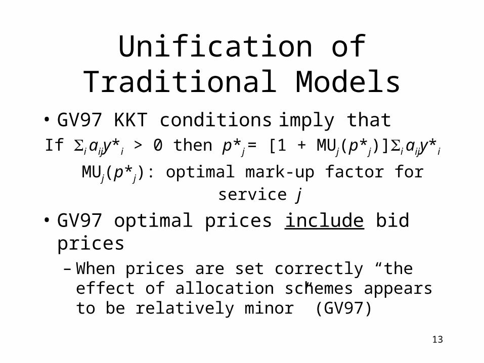
• GV97 KKT conditions imply thatIf i aijy*i > 0 then p*j = [1 + MUj(p*j)]i aijy*i

MUj(p*j): optimal mark-up factor for service j

• GV97 optimal prices include bid prices– When prices are set correctly “the effect of

allocation schemes appears to be relatively minor” (GV97)

14

Unification of Traditional Models

• Extending a result reported by Boyd and Bilegan (2003) the GV97 model can be decomposed into– A Lagrangian dual pricing problem

max i vi()s.t. i ij 0, j

– And a set of Lagrangian allocation subproblems, i

vi() maxx j ijxij

s.t. j aijxij ci

0 xij E[Nj (j)], jwith pj = i ij

15

Unification of Traditional Models

• The traditional price-proration approach combined with local optimizations can be used with the GV97 model– EMSR-based virtual nesting– DP-based bid price tables

• Ignoring demand uncertainty, pricing is more important than inventory control

• But inventory control remains important to account for demand uncertainty in between re-optimizations

16

Extension of Traditional Models

• The following contract-type is the basic modeling entity for the class of B2B problems with rentable resources– Start time and duration– Set of services requiring the usage of multiple

resources– Service prices and quantities– Take-or pay terms and conditions

• The firm structures its commercial agreements as contract-type instances (CTIs)

• The firm observes demand for CTIs

17

Extension of Traditional Models

• CTIs have overlapping booking and service periods

18

Extension of Traditional Models

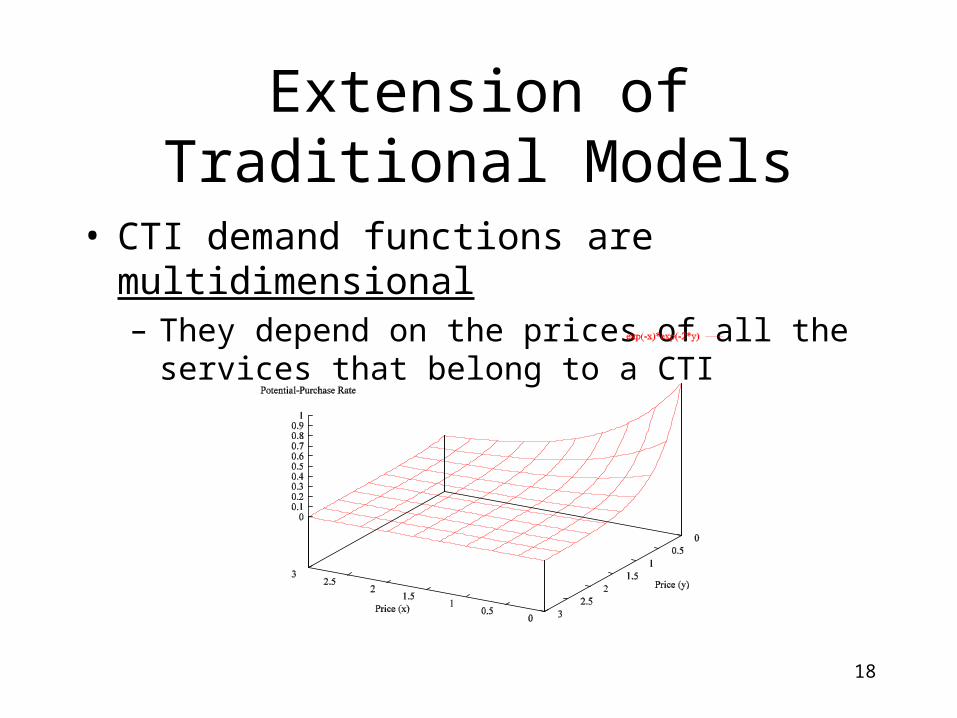
• CTI demand functions are multidimensional– They depend on the prices of all the services that

belong to a CTI

19

Extension of Traditional Models

• A time-and-space network optimization model is needed– Airline case: spatial network problem

– Hotel/Rental-car case: temporal network problem

• In most applications the variable cost of providing a B2B service can be substantial– The marginal cost may also depend on the remaining

available capacity

• B2B request size is not unitary

20

Extension of Traditional Models

• Index sets: CTI set J, service set M, resource set I, time-period set K

• Parametersj: Length of CTI j service periodNjk(pjk): r.v. # of CTI j requests received in booking period k as a

function of the price vector pjk (pjkm, m M)Sjkm: r.v. size of service m asked for by one CTI j request in period kaik’m: consumption of resource i by service m in service period k’cik’: resource i available capacity in period k’fc

ik: resource i convex variable-cost function in period k’• Decisions variables

xjk: number of accepted CTI j requests in period kpjkm: price of service m for CTI j in period k

21

Extension of Traditional Models

• Deterministic network pricing model

maxp,x j,k,m jpjkmE[Sjkm]xjk – i,k’ fcik’(Aik’)

s.t. j,k,m aik’mE[Sjkm]xjk cik’, i, k’; (yik’)

0 xjk E[Njk(pjk)], j, k

pjkm 0, j, k, m

with Aik’ j,k,m aik’mE[Sjkm]xjk

• At optimality variables xjk can be eliminated

22

Extension of Traditional Models

• Main differences with respect to GV97– Capacity constraints are “2-dimensional” (i and

k’)– Objective includes a cost function– Objective and capacity constraints include

expected service request size

23

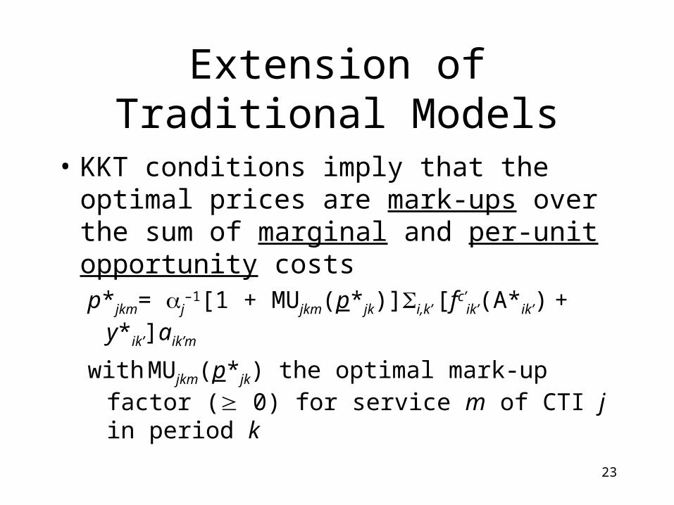
Extension of Traditional Models

• KKT conditions imply that the optimal prices are mark-ups over the sum of marginal and per-unit opportunity costsp*jkm= j

–1[1 + MUjkm(p*jk)]i,k’ [fc’ik’(A*ik’) +

y*ik’]aik’m

with MUjkm(p*jk) the optimal mark-up factor ( 0) for service m of CTI j in period k

24

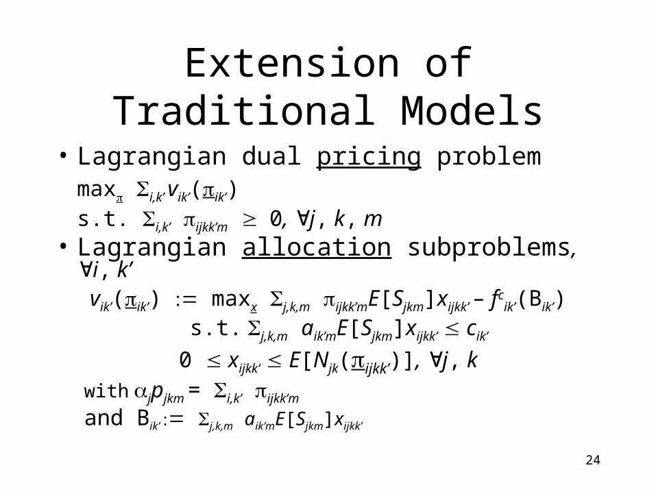
Extension of Traditional Models

• Lagrangian dual pricing problemmax i,k’ vik’(ik’)s.t. i,k’ ijkk’m 0, j, k, m

• Lagrangian allocation subproblems, i, k’vik’(ik’) maxx j,k,m ijkk’mE[Sjkm]xijkk’ – fc

ik’(Bik’)s.t. j,k,m aik’mE[Sjkm]xijkk’ cik’

0 xijkk’ E[Njk(ijkk’)], j, kwith jpjkm = i,k’ ijkk’m

and Bik’ j,k,m aik’mE[Sjkm]xijkk’

25

Extension of Traditional Models

• The following traditional scheme applies– Solve the network (pricing) model to compute

optimal prices and capacity duals– Compute resource/time-period combinations

capacity value functions– Use these parameters to instantiate a control

policy

26

Possible Types of Control Policies

• Auction-based one-to-many negotiations– Set a minimum price for a block of capacity-to-

auction to cover variable and opportunity costs

• Bilateral negotiations– First set unit prices according to the

optimization model then negotiate sizes– Set size-dependent prices to maximize the

expected profitability of the transaction

27

Possible Types of Control Policies

• Bilateral negotiation with size-dependent prices– Consider a request for services {m} with sizes {skm}

and service time-periods {k’} of length received in time period k < k’

– Assume feasible sizes {skm}

• The quoted prices {Pkm} should

– Cover the incremental cost IC(sk) of accommodating the request

– Account for the buyer’s willingness to pay or valuation

28

Possible Types of Control Policies

IC(sk) i,k’ [VCik’(sk) + OCik’(sk)]

VCik’(sk): Variable cost of resource i in period k’ with cb

ik’ already booked capacity

VCik’(sk) fcik’ (cb

ik’ + j,k,m aik’mskm) – fcik’ (cb

ik’)

OCik’(sk): Approximate opportunity cost of resource i in period k’, e.g.

OCik’(sk) m aik’mskmy*ik’

29

Possible Types of Control Policies

• Given the incremental cost, compute prices to maximize expected profit

maxP [m Pkmskm – IC(sk)] Pr(m{Wm

Pkm})

With Wm the random variable buyer’s willingness to pay for service m

30

Possible Types of Control Policies

• Given the incremental cost, compute total revenue to maximize expected profit

maxR [R – IC(sk)] Pr(V R)R: the total revenue from the transactionV: the buyer’s valuation or budget random

variable

• Prices can be recovered by splitting R according to some business rule

31

Conclusions

• Contributions– Introduced the class of B2B problems with

rentable resources– Unified and extended traditional models

• Additional research– CTI demand modeling/forecasting and

interplay with optimization/control-policies– Numerical, experimental or empirical testing