1 Modeling and Simulation of Beam Control Systems Part 1. Foundations of Wave Optics Simulation.

1

Modeling and Simulation of Beam Control Systems

Part 1. Foundations of Wave Optics Simulation

2

Introduction & Overview


Part 2. Modeling Optical Effects

Lunch

Part 3. Modeling Beam Control System Components

Part 4. Modeling and Simulating Beam Control Systems

Discussion

Agenda

3


In Part 1 we will review all the basic theory most important to the modeling and simulation of beam control systems. We will be covering a lot of ground in a limited time.


For those already familiar with the basic theory, Part 1 should be useful from the standpoint of introducing our notation and conventions.


For those already familiar with the basic theory, Part 1 should be useful from the standpoint of introducing our notation and conventions.

Also we will be introducing two unconventional analytic devices: (1) an operator notation for Fourier optics, and (2) ray sets, used to take into account geometric constraints.

4

Overview

Scalar Diffraction Theory and Fourier Optics

The Discrete Fourier Transform

Optical Effects of Atmospheric Turbulence

Special Topics

Foundations of Wave Optics Simulation

5

Foundations of Wave Optics SimulationOverview Scalar diffraction theory and Fourier optics are the theoretical foundations of wave

optics simulation. These involve certain simplifying assumptions which are not strictly satisfied for all cases of interest, but the theory can be extended.

The Discrete Fourier Transform, or DFT, is the computational workhorse of wave optics simulation. It is important to take into account the properties of the DFT when choosing mesh spacings, mesh dimensions, and filtering techniques.

The optical effects of atmospheric turbulence can strongly affect the performance of beam control systems involving long distance propagation through the atmosphere. They are therefore very important in the design and modeling of such systems.

Other special topics relevant to the modeling and simulation of beam control systems include polarization and birefringence, partial coherence, incoherent imaging, refractive bending, and reflection from optically rough surfaces.

6

Scalar Diffraction Theory

The Huygens-Fresnel Principle

The Fresnel Approximation

Fourier Optics

Waves vs. Rays

Extending Scalar Diffraction Theory

Scalar Diffraction Theory and Fourier Optics

Reference: An Introduction to Fourier Optics, by Joseph Goodman

7

Scalar Diffraction Theory

/

phase

amplitude

field optical

)()()( where

c

A

u

rierAru

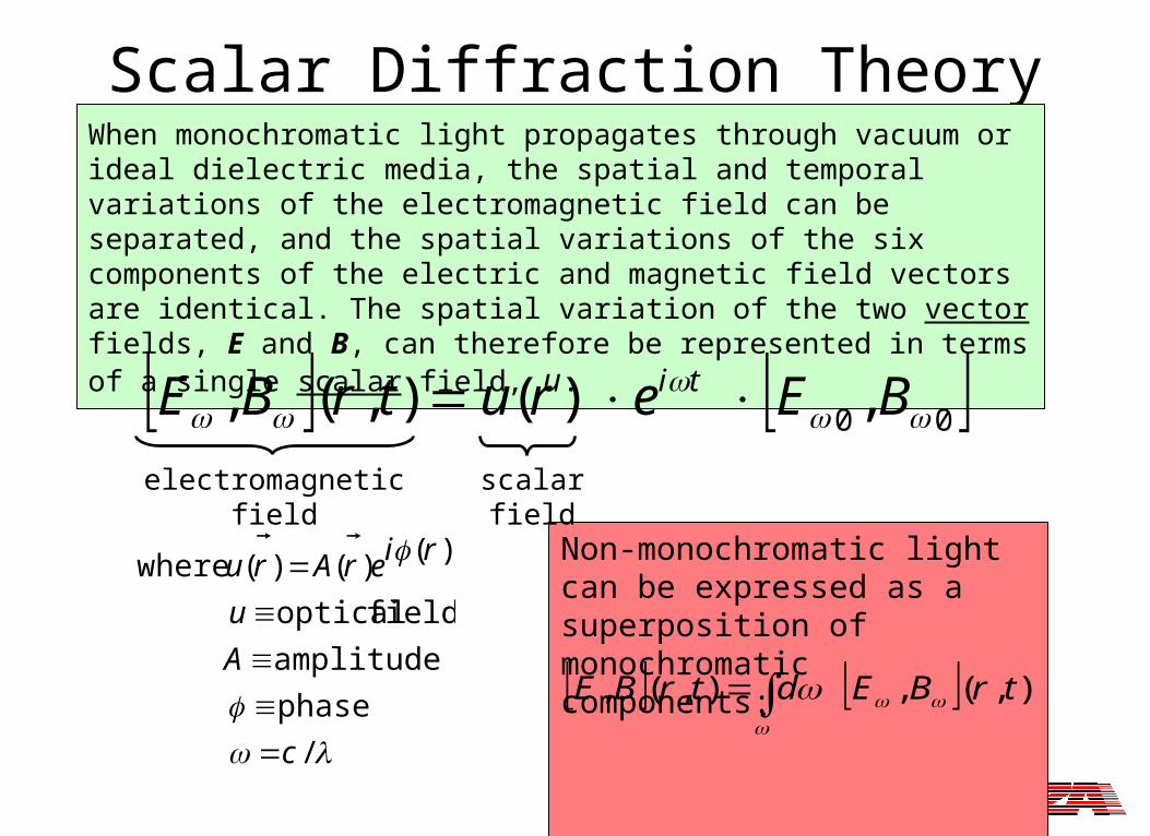
When monochromatic light propagates through vacuum or ideal dielectric media, the spatial and temporal variations of the electromagnetic field can be separated, and the spatial variations of the six components of the electric and magnetic field vectors are identical. The spatial variation of the two vector fields, E and B, can therefore be represented in terms of a single scalar field, u.

Non-monochromatic light can be expressed as a superposition of monochromatic components:

),(, ),(, trBEdtrBE

scalar field

00 , )( ),(,

BEerutrBE ti

electromagnetic field

8

The Huygens-Fresnel Principle

12

22

12

22221111

1112

22

2

];,[ ],;,[

where

cos 1

1

zzz

zR

k

zyxzyx

R

ikRed

iuu

z1 z2

u1

u2

R1

2

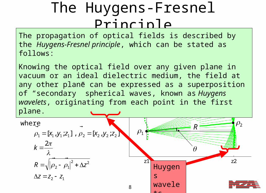
The propagation of optical fields is described by the Huygens-Fresnel principle, which can be stated as follows:

Knowing the optical field over any given plane in vacuum or an ideal dielectric medium, the field at any other plane can be expressed as a superposition of “secondary” spherical waves, known as Huygens wavelets, originating from each point in the first plane.

Huygens wavelets

9

The Fresnel Approximation

1cos

2exp

112

1

, assume weIf

cos ,

2

12

2

1222

12

12

1112

222

z

ikzikeikRe

zR

zzzR

z

R

ikRed

i

zikeyx uu

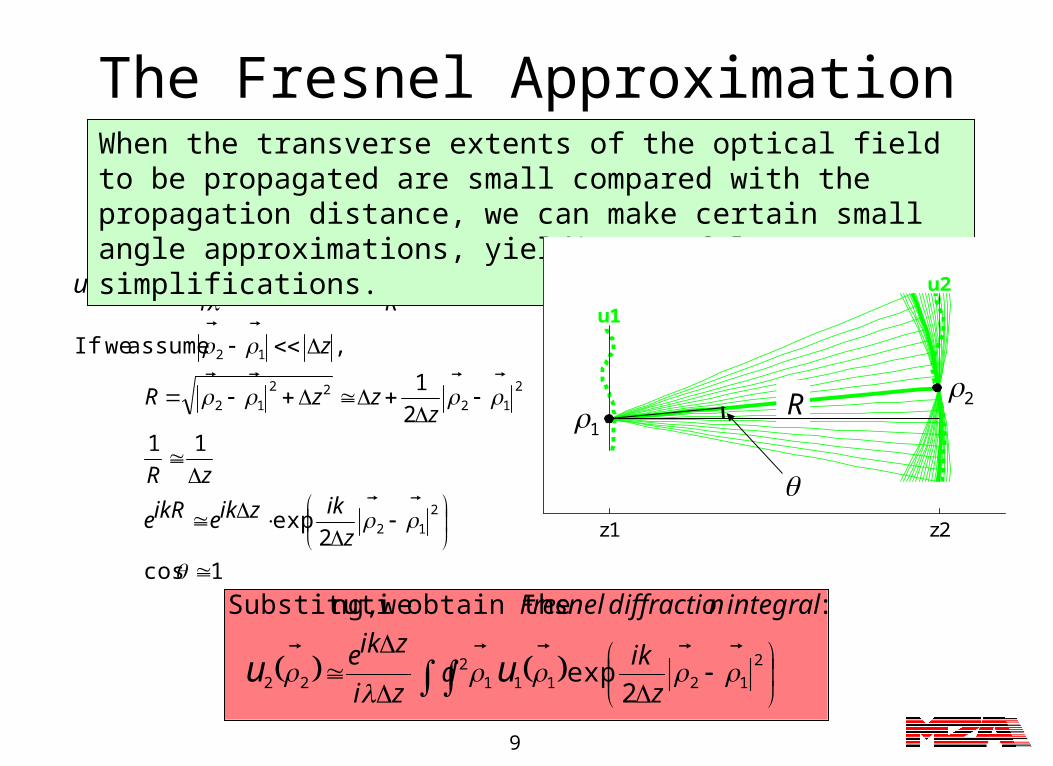
When the transverse extents of the optical field to be propagated are small compared with the propagation distance, we can make certain small angle approximations, yielding useful simplifications.

2

121112

22 2exp

: obtain the weng,Substituti

z

ikd

zi

zike

integral ndiffractio Fresnel

uu

z1 z2

u1

u2

R1

2

10

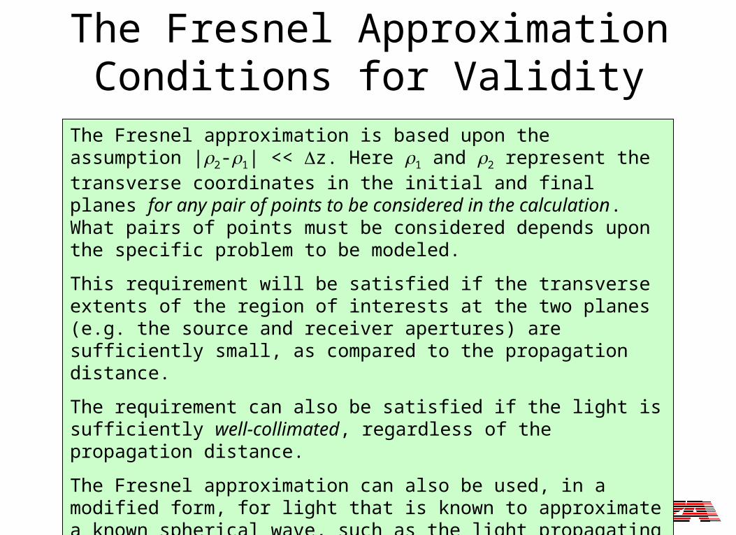
The Fresnel ApproximationConditions for Validity

The Fresnel approximation is based upon the assumption |2-1| << z. Here 1 and 2 represent the transverse coordinates in the initial and final planes for any pair of points to be considered in the calculation. What pairs of points must be considered depends upon the specific problem to be modeled.

This requirement will be satisfied if the transverse extents of the region of interests at the two planes (e.g. the source and receiver apertures) are sufficiently small, as compared to the propagation distance.

The requirement can also be satisfied if the light is sufficiently well-collimated, regardless of the propagation distance.

The Fresnel approximation can also be used, in a modified form, for light that is known to approximate a known spherical wave, such as the light propagating between the primary and secondary mirrors of a telescope.

11

uFU

zUzi

zikeuF

uz

iFz

i

z

ikud

zi

zikeu

f

fz

z

where

expexp

2exp

112

12

2

2

121112

22

quadratic phase factor

Fourier Optics

scaled Fourier transform

When the Fresnel approximation holds, the Fresnel diffraction integral can be decomposed into a sequence of three successive operations:

1. Multiplication by a quadratic phase factor

2. A Fourier transform (scaled)

3. Multiplication by a quadratic phase factor.

quadratic phase factor

12

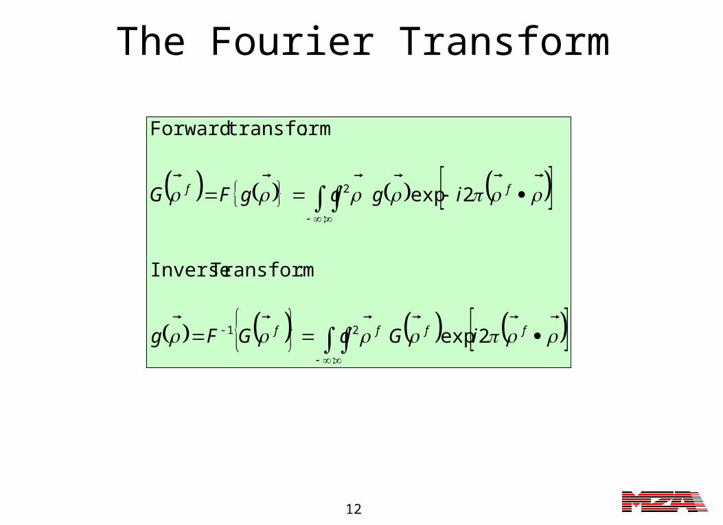
The Fourier Transform

ffff

ff

iGdGFg

igdgFG

2exp

:Transform Inverse

2exp

: transformForward

:

21

:

2

13

z1 z2

u1

u2

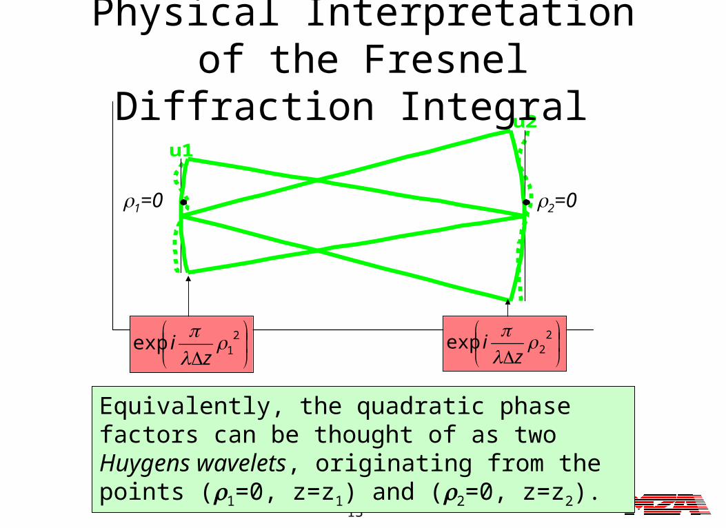
Physical Interpretation of the Fresnel Diffraction Integral

The two quadratic phase factors appearing in the Fresnel diffraction integral correspond to two confocal surfaces.

2

2exp

zi

2

1exp

zi

1=0 2=0

Equivalently, the quadratic phase factors can be thought of as two Huygens wavelets, originating from the points (1=0, z=z1) and (2=0, z=z2).

14

Fourier Optics in Operator Notation

zzzz

zz

z

z

zzz

z

uFu

uz

iu

u

u

uz

iFz

iu

QFQP

F

Q

P

QFQ

exp

where

expexp

2

11

11

1122

22

For notational convenience it is sometimes useful to express Fourier optics relationships in terms of linear operators. We will use Pz, to indicate propagation, Fz for a scaled Fourier transform, and Qz for multiplication by a quadratic phase factor.

221

1

112

uuu

uuu

zz

zzzz

PP

QFQP

15

zz

uuu

i

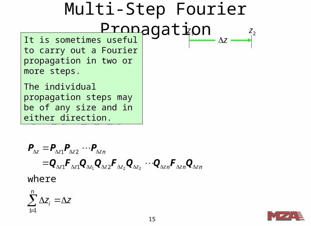
nznznzzzzzzz

nzzzz

zzzz

n

1i

211

21

112

where

221

QFQQFQQFQ

PPPP

QFQP

Multi-Step Fourier PropagationIt is sometimes useful to carry out a Fourier propagation in two or more steps.

The individual propagation steps may be of any size and in either direction.

z

z1 z2

z1 z2

16

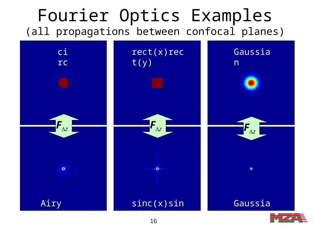
Fourier Optics Examples(all propagations between confocal planes)

circ Gaussian

sinc(x)sinc(y)Airy pattern

rect(x)rect(y)

Gaussian

Fz Fz Fz

17

Waves vs. RaysScalar diffraction theory and Fourier optics are usually described in terms of waves or fields, but they can also be described, with equal rigor, in terms of rays.

This may seem surprising, because rays are constructs more typically associated with geometric optics, as opposed to wave optics. In geometric optics, rays are thought of as carrying a energy, or intensity, possibly distributed over a range of wavelengths. In wave optics, each ray must be thought of as carrying a certain complex amplitude, at a specific wavelength.

The advantage of thinking in terms of rays, as opposed to waves or fields, is that it makes it easier to take into account geometric considerations, such as limiting apertures. A wave can be thought of as a set of rays, and geometric considerations may allow us to restrict our attention to a smaller subset of that set.

18

z1 z2

u1

u2

z1 z2

u1

u2

z1 z2

u1

u2

From the Huygens-Fresnel principle, any (scalar) light wave can be decomposed into a set of spherical waves (Huygen’s wavelets) originating from all the points on one plane, z1.

Each Huygen’s wavelet can be further decomposed into a set of rays, connecting the origination point 1 on the plane z1with all points on

some other plane z2.

Each ray defines the contribution from a point source at 1 to the field

at a specific point 2 on the plane z2. Conversely, the same ray also defines the contribution from a point source at 2 to the field at 1.

z1 z2

u1

u2

z1 z2

u1

u2

Suppose we now collect all the rays impinging on the point z2 from all points in the first plane. This set of rays is equivalent to a Huygen’s wavelet, this time originating at the point 2 and going backwards.

Repeating the procedure for all points in the any (scalar) light wave can be decomposed into a set of spherical waves (Huygen’s wavelets) originating from all the points on one plane, z1.

A Wave as a Set of Rays

1

2

19

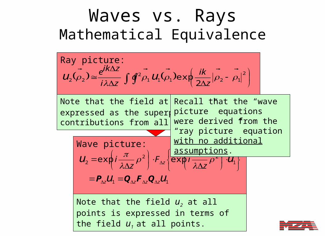
Wave picture:

11

122

2

expexp

uu

uu

zzzz

z ziF

zi

QFQP

Waves vs. RaysMathematical Equivalence

Ray picture:

2

121112

22 2exp

z

ikd

zi

zike uu

Note that the field u2 at all points is expressed

in terms of the field u1 at all points.

Note that the field at each point 2 is expressed as the superposition of the contributions from all points 1.

Recall that the “wave picture” equations were derived from the “ray picture” equation with no additional assumptions.

20

Waves vs. RaysWhy the “Ray Picture” is Useful

Thinking of light as being made up of rays, as opposed to waves or fields, makes it easier to take into account a priori geometric constraints pertaining to two or more planes at the same time.

For example, if the light to be modeled is known to pass through a limiting apertures, we can restrict our attention to just the set of the rays that pass through that aperture.

Similarly, if there are multiple limiting apertures, we can restrict our attention to the intersection of the ray sets defined by the individual apertures.

It is important to understand that strictly speaking a given ray set remains well-defined only within a contiguous volume filled with a uniform dielectric medium, and only for purely monochromatic light.

21

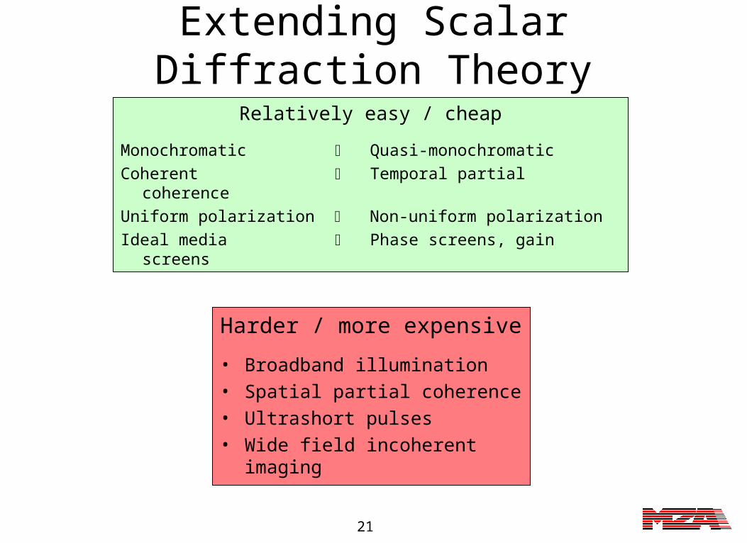
Extending Scalar Diffraction Theory

Relatively easy / cheap

Monochromatic Quasi-monochromatic

Coherent Temporal partial coherence

Uniform polarization Non-uniform polarization

Ideal media Phase screens, gain screens

Harder / more expensive

• Broadband illumination

• Spatial partial coherence

• Ultrashort pulses

• Wide field incoherent imaging

22

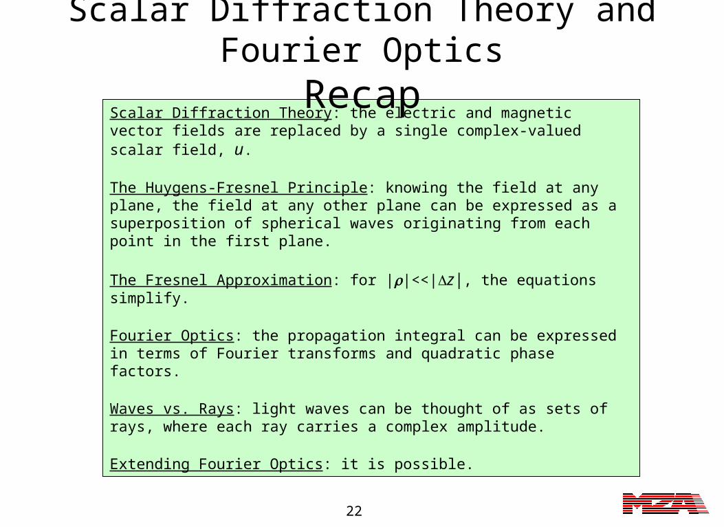
Scalar Diffraction Theory: the electric and magnetic vector fields are replaced by a single complex-valued scalar field, u.

The Huygens-Fresnel Principle: knowing the field at any plane, the field at any other plane can be expressed as a superposition of spherical waves originating from each point in the first plane.

The Fresnel Approximation: for ||<<|z|, the equations simplify.

Fourier Optics: the propagation integral can be expressed in terms of Fourier transforms and quadratic phase factors.

Waves vs. Rays: light waves can be thought of as sets of rays, where each ray carries a complex amplitude.

Extending Fourier Optics: it is possible.

Scalar Diffraction Theory and Fourier OpticsRecap

23

What happens when we try to represent a continuous complex field on a finite discrete mesh?

How can we reconstruct the continuous field from the discrete mesh?

How can we ensure that the results obtained will be correct?

What can go wrong?

The Discrete Fourier Transform

Reference: The Fast Fourier Transform, by Oran Brigham

2exp1

:(DFT) ansformFourier tr Discrete

2exp

:ansformFourier tr

1 1,,,2,','

:

2

N

j

N

kji

fjijiDjiDD

fjiD

ff

igN

gFG

igdgFG

24

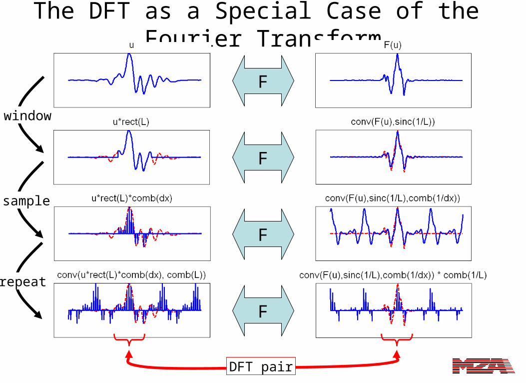
The DFT as a Special Case of the Fourier Transform

window

F

F

F

F

sample

repeat

DFT pair

25

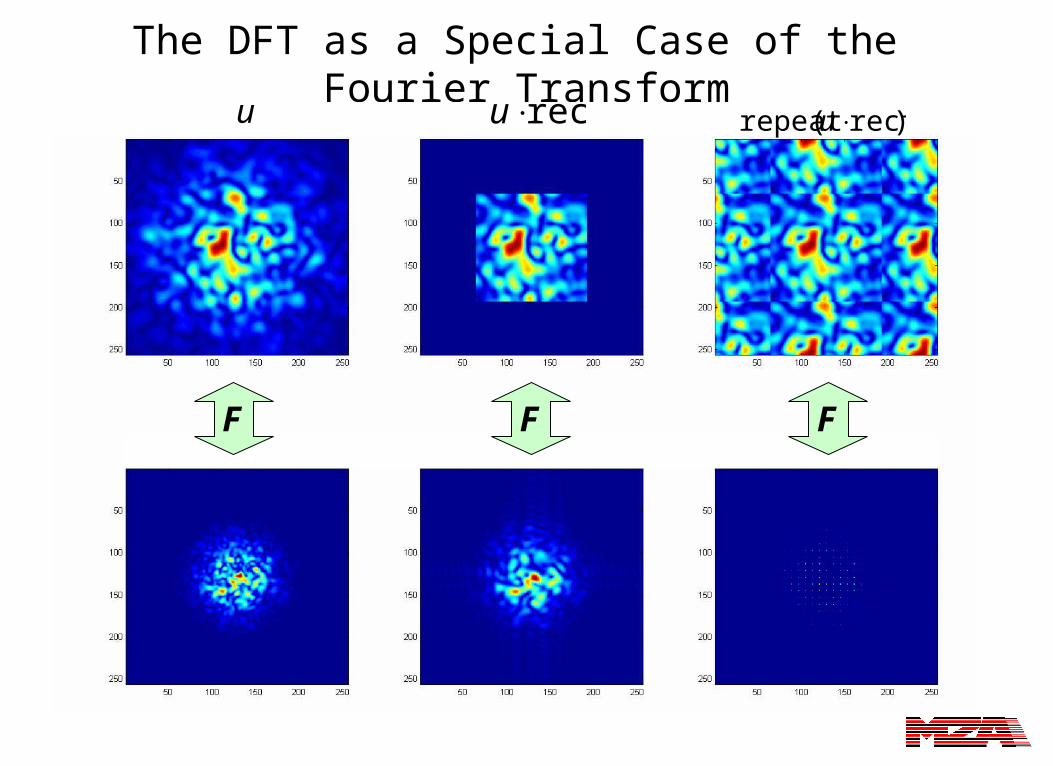
The DFT as a Special Case of the Fourier Transform

rectuu )rect(repeat u

F F F

26

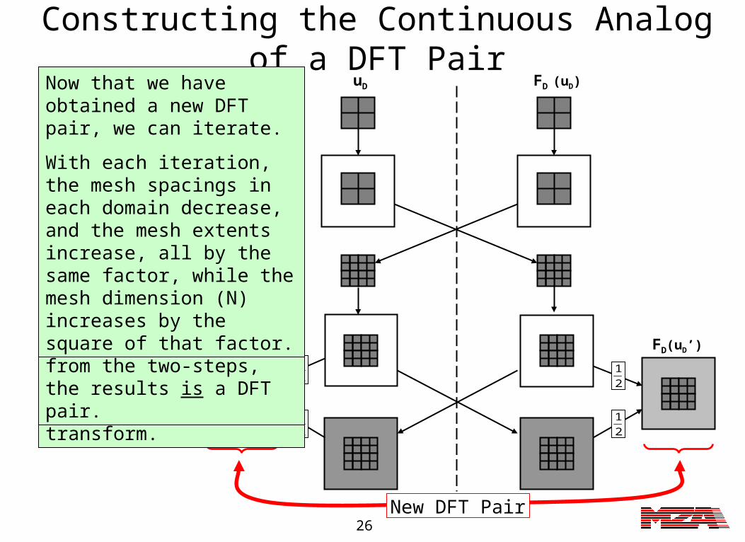
Constructing the Continuous Analog of a DFT Pair

uD FD (uD)

FD(uD’) uD’

2

12

1

2

1

2

1

New DFT Pair

When using DFTs, in order to minimize the computational requirements, one often chooses to make the mesh spacing as large as possible while still obtaining correct results. (Nyquist Criterion)

Sometimes it is useful to construct a more densely sampled version of the function and/or its transform.

One way to do this do this is to use Fourier interpolation:

To interpolate the function, zero-pad its transform, then compute the inverse DFT.

To interpolate the transform, zero-pad the function, then compute the DFT.

If one applies Fourier interpolation to both a function and its DFT transform, the resulting interpolated versions do not form a DFT pair.

However if we then perform a second Fourier interpolation in each domain and average the results from the two-steps, the results is a DFT pair.

Now that we have obtained a new DFT pair, we can iterate.

With each iteration, the mesh spacings in each domain decrease, and the mesh extents increase, all by the same factor, while the mesh dimension (N) increases by the square of that factor.

27

Constructing the Continuous Analog of a DFT Pair

Example: A Discrete “Point Source” N=16 N=64 N=256

u

F(u)

28

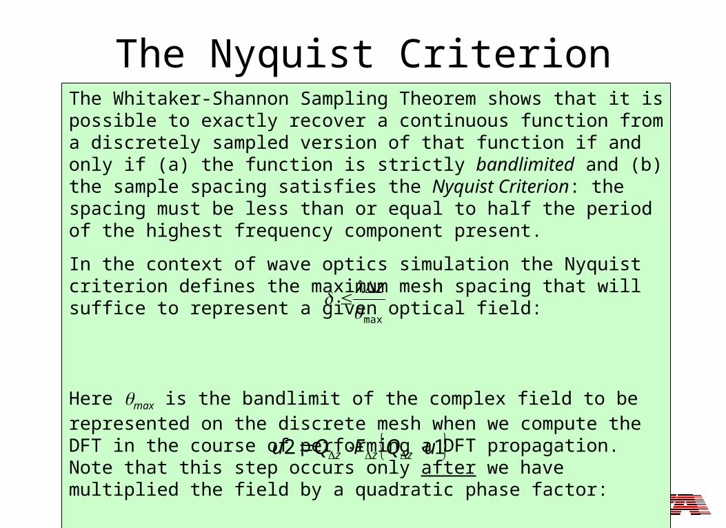
The Whitaker-Shannon Sampling Theorem shows that it is possible to exactly recover a continuous function from a discretely sampled version of that function if and only if (a) the function is strictly bandlimited and (b) the sample spacing satisfies the Nyquist Criterion: the spacing must be less than or equal to half the period of the highest frequency component present.

In the context of wave optics simulation the Nyquist criterion defines the maximum mesh spacing that will suffice to represent a given optical field:

Here max is the bandlimit of the complex field to be represented on the discrete mesh when we compute the DFT in the course of performing a DFT propagation. Note that this step occurs only after we have multiplied the field by a quadratic phase factor:

The Nyquist Criterion

12 uQFQu zzz

max z

29

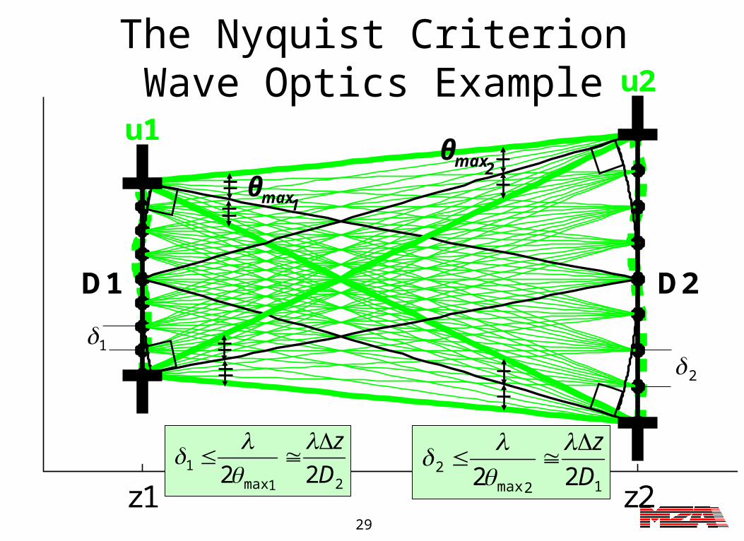
z1 z2

u1

u2

D1 D2

21max1 22

D

z

2 1

1maxθ2maxθ

12max2 22

D

z

The Nyquist CriterionWave Optics Example

30

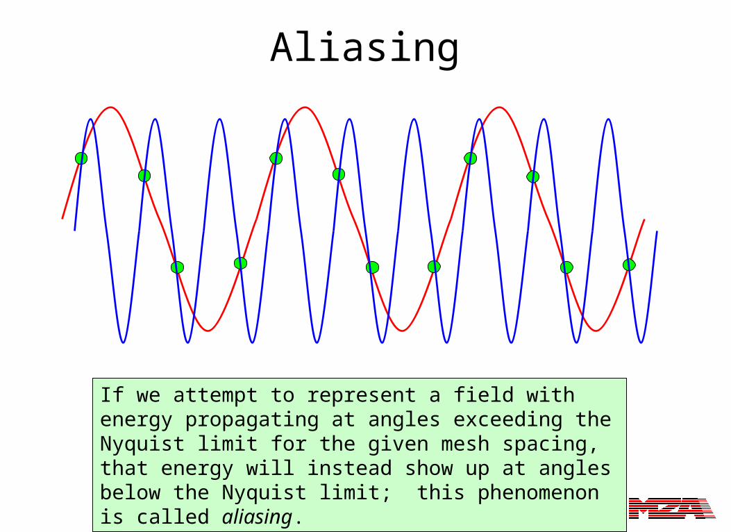
Aliasing

If we attempt to represent a field with energy propagating at angles exceeding the Nyquist limit for the given mesh spacing, that energy will instead show up at angles below the Nyquist limit; this phenomenon is called aliasing.

31

The Discrete Fourier Transform - Recap

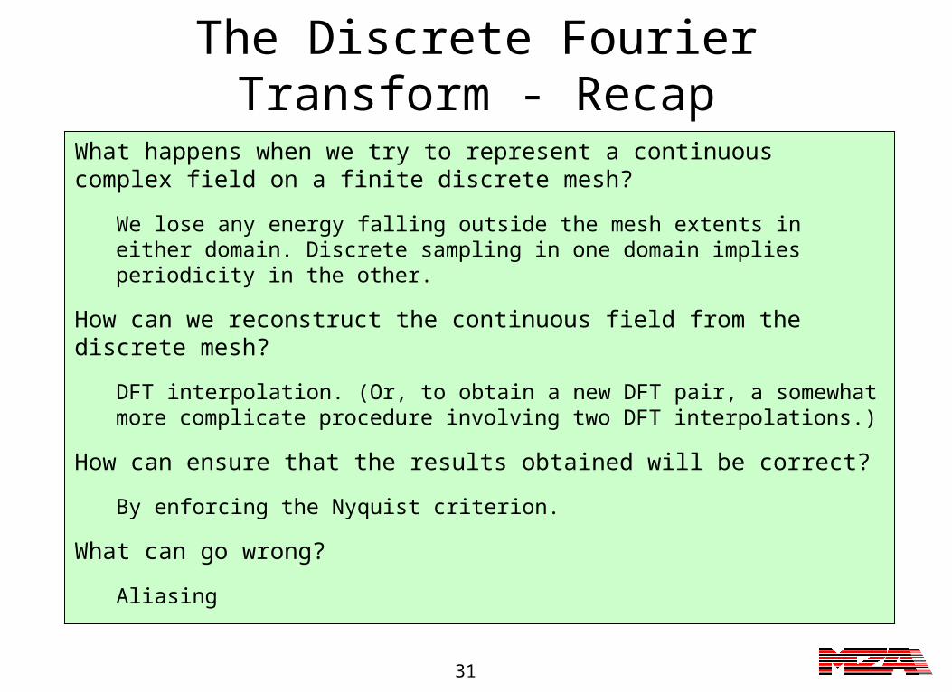
What happens when we try to represent a continuous complex field on a finite discrete mesh?

We lose any energy falling outside the mesh extents in either domain. Discrete sampling in one domain implies periodicity in the other.

How can we reconstruct the continuous field from the discrete mesh?

DFT interpolation. (Or, to obtain a new DFT pair, a somewhat more complicate procedure involving two DFT interpolations.)

How can ensure that the results obtained will be correct?

By enforcing the Nyquist criterion.

What can go wrong?

Aliasing

32

Optical Effects of Atmospheric Turbulence

Topics• Nature and magnitude of the turbulence• Quantitative description of the turbulence

– Spatial and temporal characteristics

• Qualitative description of optical effects• Quantitative description of optical effects

– Modified wave equation, approximate solution methods

– Key statistical quantities: irradiance variance, r0, 0 , Strehl

– Sampling of analytical results (simple formulas)

• Preview of numerical simulation methods – Segmentation of path, phase “screens”, sequential propagation model

• Summary of key assumptions

33

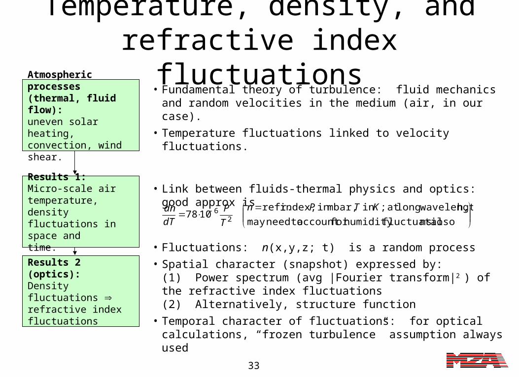
Temperature, density, and refractive index fluctuations

Results 2 (optics):Density fluctuations refractive index fluctuations

Results 1:Micro-scale air temperature, densityfluctuations in space andtime.

Atmospheric processes(thermal, fluid flow):uneven solar heating, convection, wind shear.

also nsfluctuatiohumidity for account toneedmay

h, wavelengtlongat ;in mbar,in index, refr.1078

26 KTPn

T

P

dT

dn

• Fundamental theory of turbulence: fluid mechanics and random velocities in the medium (air, in our case).

• Temperature fluctuations linked to velocity fluctuations.

• Fluctuations: n(x,y,z; t) is a random process

• Spatial character (snapshot) expressed by:(1) Power spectrum (avg |Fourier transform|2 ) of the refractive index fluctuations(2) Alternatively, structure function

• Temporal character of fluctuations: for optical calculations, “frozen turbulence” assumption always used

• Link between fluids-thermal physics and optics: good approx is

34

Spatial character of fluctuations (1)

• In space-domain, fluctuations of refractive index, n, can be characterized by the structure

function, Dn(r), where r = separation (m) between two points

• For any random process g(r) that is stationary and isotropic, structure function is defined by

strength turbi.e.,

constant, structureindex refr.

)(2

322

n

nn

C

rCrD

• The Kolmogorov model of turbulence leads to

separation of fnc as diff, theof variance:diffsqr -mean a is

n valueexpectatio,)()()()( 211

D

rDrDrrgrg gg

• The Kolmogorov model is valid for an intermediate range of r :

l0 < r < L0 , between the “inner scale” and “outer scale” • Calculations (analytical and sim) of optical propagation through turbulence are usually

done by using frequency-domain characterization of the index fluctuations: power spectral density (power spectrum, PSD) corresponding to Dn(r)

1.00007

1.00026

nair (ignore

dispersion)

2.4E-91.1E-96E-18 m-2/340 kft

4.6E-8

[Dn(10cm)]

1E-14 m-2/3

Cn2

gnd

altitude

Numerical examples, for typical Cn2 values

1.0E-7

[Dn(1 m)]

1.00007

1.00026

nair (ignore

dispersion)

2.4E-91.1E-96E-18 m-2/340 kft

4.6E-8

[Dn(10cm)]

1E-14 m-2/3

Cn2

gnd

altitude

Numerical examples, for typical Cn2 values

1.0E-7

[Dn(1 m)]

35

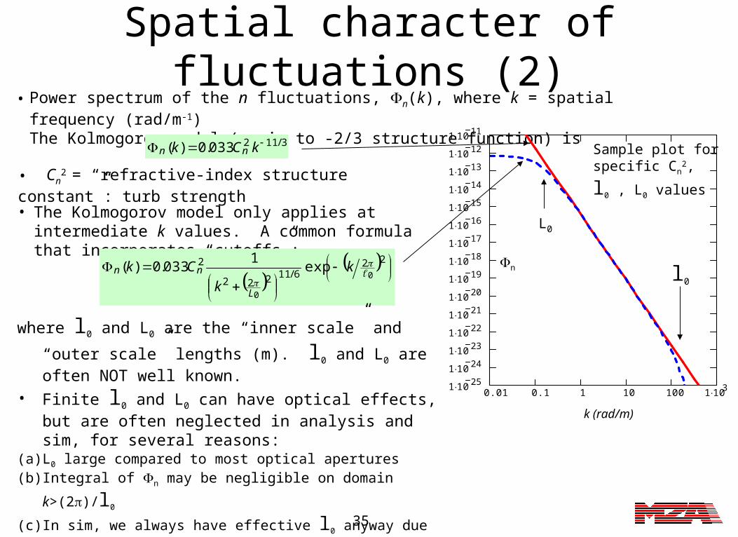
Spatial character of fluctuations (2)

• Power spectrum of the n fluctuations, n(k), where k = spatial frequency (rad/m-1)The Kolmogorov model (equiv to -2/3 structure function) is

3/112033.0)( kCk nn

• The Kolmogorov model only applies at intermediate k values. A common formula that incorporates “cutoffs”:

22

6/11222

20

0

exp1

033.0)(

k

k

Ck

L

nn

where l0 and L0 are the “inner scale” and “outer scale” lengths

(m). l0 and L0 are often NOT well known.

• Finite l0 and L0 can have optical effects, but are often neglected in analysis and sim, for several reasons:

(a) L0 large compared to most optical apertures

(b) Integral of n may be negligible on domain k>(2)/l0

(c) In sim, we always have effective l0 anyway due to computational grid step size

(d) Values not well known

• Cn2 = “refractive-index structure constant”: turb strength

0.01 0.1 1 10 100 1 1031 10 25

1 10 24

1 10 23

1 10 22

1 10 21

1 10 20

1 10 19

1 10 18

1 10 17

1 10 16

1 10 15

1 10 14

1 10 13

1 10 12

1 10 11

k (rad/m)

n l0

L0

Sample plot for

specific Cn2, l0 , L0

values

36

Optical effects - qualitative• Wave prop speed: c=c0/n

(c0 = vacuum), so n c

• Along prop path– First effect: some segments of wavefront

(WF) are retarded relative to others

– Second effect: resulting local focusing generates irradiance fluctuations

• In focal (image plane)– WF distortions and, to much lesser degree,

irradiance fluctuations across receiver aperture (pupil) cause

• Broadening of point spread function (PSF)

• Lowering of peak irradiance

– Practical significance

• Degrades image resolution

• May reduce image irradiance below noise

• Similar effects in beam projection as in imaging

prop direction

wavefronts become progressively more distorted, and irradiance begins to vary

Imaging system

image plane irradiance(PSF) without

turbwithturb

turb region

unperturbed wavefront (surface of constant phase), suppose from distant point src

37

Profiles of Cn2

• In previous formulas (structure function and PSD), Cn

2 was a constant: random n process assumed statistically stationary

• This is certainly not true over large distances in the atmosphere: assume “locally stationary” random process, i.e., slowly-varying average properties modulate the turbulence spectrum.

• Mathematical representation of “locally stationary”:

3/112 )(033.0);( kzCzk nn

• Cn2(z) slowly-varying function of distance along prop

path; in particular, strong variation of Cn2(z) with

altitude.In general, also have l0(z) and L0(z).

• Vertical profile Cn2(h) is a key empirical input to most

turbulence calculations. Various average-profile models exist, but nature varies a lot around the standard models: spatial layering, temporal intermittency. Plot shows 4 models:

0 5 10 15 20 251 10

19

1 1018

1 1017

1 1016

1 1015

1 1014

1 1013

AMOSClear-1Clear-2HV5/7

AMOS, CLEAR1&2, HV5/7 Cn2 Profiles

Altitude (km MSL)

Cn2

(m

^-2/

3)

38

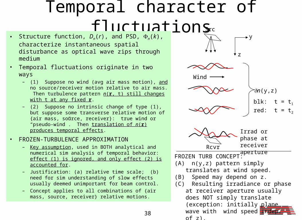
Temporal character of fluctuations

• Structure function, Dn(r), and PSD, n(k), characterize instantaneous spatial disturbance as optical wave zips through medium

• Temporal fluctuations originate in two ways– (1) Suppose no wind (avg air mass motion), and no

source/receiver motion relative to air mass. Then turbulence pattern n(r, t) still changes with t at any fixed r.

– (2) Suppose no intrinsic change of type (1), but suppose some transverse relative motion of {air mass, source, receiver}: true wind or “pseudo-wind”. Then translation of n(r) produces temporal effects.

• FROZEN-TURBULENCE APPROXIMATION– Key assumption, used in BOTH analytical and

numerical sim analysis of temporal behavior: effect (1) is ignored, and only effect (2) is accounted for.

– Justification: (a) relative time scale; (b) need for sim understanding of slow effects usually deemed unimportant for beam control.

– Concept applies to all combinations of {air mass, source, receiver} relative motions.

FROZEN TURB CONCEPT:(A) n(y,z) pattern simply translates at wind

speed.(B) Speed may depend on z.(C) Resulting irradiance or phase at receiver

aperture usually does NOT simply translate (exception: initially plane wave with wind speed indep. of z).

blk: t = t1

red: t = t2

z

y

n(y,z)

Src

Rcvr

Wind

Irrad or phase at receiver aperture

39

Fundamental theory for prop through turbulence (1)

• Wave equation (monochromatic) for vacuum or uniform dielectric medium

• Wave equation in presence of fluctuations n(x,y,z; t): third term couples the polarizations during propagation

• Fundamental approximation: order of magnitude calculations imply that the coupling term is negligible.In this approx, the fluctuations do not mix polarization components Turbulent prop still satisfies the “scalar diffraction” picture.Resulting equation, with extra decomposition n(r) = <n>+n(r), and letting k = k0 n0 = average wave vector in unperturbed medium

)r(iE

n

ckrEnkrE

for eqs uncoupled 3

index refr. uniform vacuum,0

000

220

2

,2

,0)()(

0)()(

)(2)()()( 22

02

rE

rn

rnrErnkrE

0)())(

21()(0

22 rEn

rnkrE

perturbation term relative to Eq (1)

(1)

(2)

(3)

40

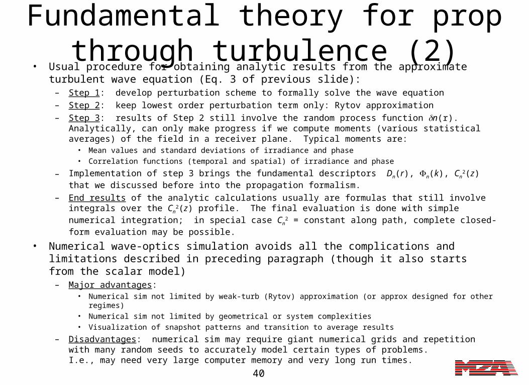
Fundamental theory for prop through turbulence (2)

• Usual procedure for obtaining analytic results from the approximate turbulent wave equation (Eq. 3 of previous slide):

– Step 1: develop perturbation scheme to formally solve the wave equation– Step 2: keep lowest order perturbation term only: Rytov approximation– Step 3: results of Step 2 still involve the random process function n(r). Analytically, can only

make progress if we compute moments (various statistical averages) of the field in a receiver plane. Typical moments are:

• Mean values and standard deviations of irradiance and phase• Correlation functions (temporal and spatial) of irradiance and phase

– Implementation of step 3 brings the fundamental descriptors Dn(r), n(k), Cn2(z) that we

discussed before into the propagation formalism.– End results of the analytic calculations usually are formulas that still involve integrals over the

Cn2(z) profile. The final evaluation is done with simple numerical integration; in special case

Cn2 = constant along path, complete closed-form evaluation may be possible.

• Numerical wave-optics simulation avoids all the complications and limitations described in preceding paragraph (though it also starts from the scalar model)

– Major advantages:• Numerical sim not limited by weak-turb (Rytov) approximation (or approx designed for other regimes)• Numerical sim not limited by geometrical or system complexities• Visualization of snapshot patterns and transition to average results

– Disadvantages: numerical sim may require giant numerical grids and repetition with many random seeds to accurately model certain types of problems. I.e., may need very large computer memory and very long run times.

41

Key statistical optics quantities

• Certain statistical quantities, which depend critically on the turbulence, are common ground of theory, numerical simulation, and optical measurements.

• Key parameters that determine optical system performance– Normalized irradiance variance (NIV), or log-amplitude variance (LAV)

– Transverse wave or phase coherence length (r0)

– Isoplanatic angle (0)

– Temporal parameters: Greenwood frequency, Tyler frequency

• Key parameters that are themselves performance measures– Strehl

– Resolution measures: half (or other) PSF width, optical transfer function (OTF)

• Subsequent slides introduce several of these parameters: these will reappear frequently in the discussion of discrete numerical methods and beam control simulation

42

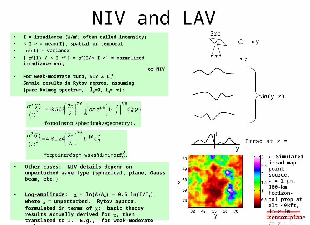
NIV and LAV• I = irradiance (W/m2; often called intensity)• < I > = mean(I), spatial or temporal• 2(I) = variance

• [ 2(I) / < I >2 ] = 2(I/< I >) = normalized irradiance var, or NIV

• For weak-moderate turb, NIV Cn2.

Sample results in Rytov approx, assuming

{pure Kolmog spectrum, l0=0, L0= }:

• Other cases: NIV details depend on unperturbed wave type (spherical, plane, Gauss beam, etc.)

• Log-amplitude: = ln(A/A0) = 0.5 ln(I/I0), where 0 = unperturbed. Rytov approx. formulated in terms of : basic theory results actually derived for , then translated to I. E.g., for weak-moderate turb, [ 2(I) / < I >2 ] 4 2() (see leading 4 in above formulas)

.2uniform and ,(sph wave) srcpoint for

261167

2

2 2124.04

)(

nC

nCLI

I

geometry). wave"spherical(" srcpoint for

)(12

563.04)(

0

265

6567

2

2

Ln zC

L

zzdz

I

I

n(y,z)

Src

Irrad at z = L

z

y

y

I

x

y

0.5

1

1.5

2

2.5

3x 10

-16

30 40 50 60 70

30

40

50

60

70

Simulated irrad map:point source, = 1 m,100-km horizon-tal prop at alt 40kft,1m x 1m sensor plane at z = L.

43

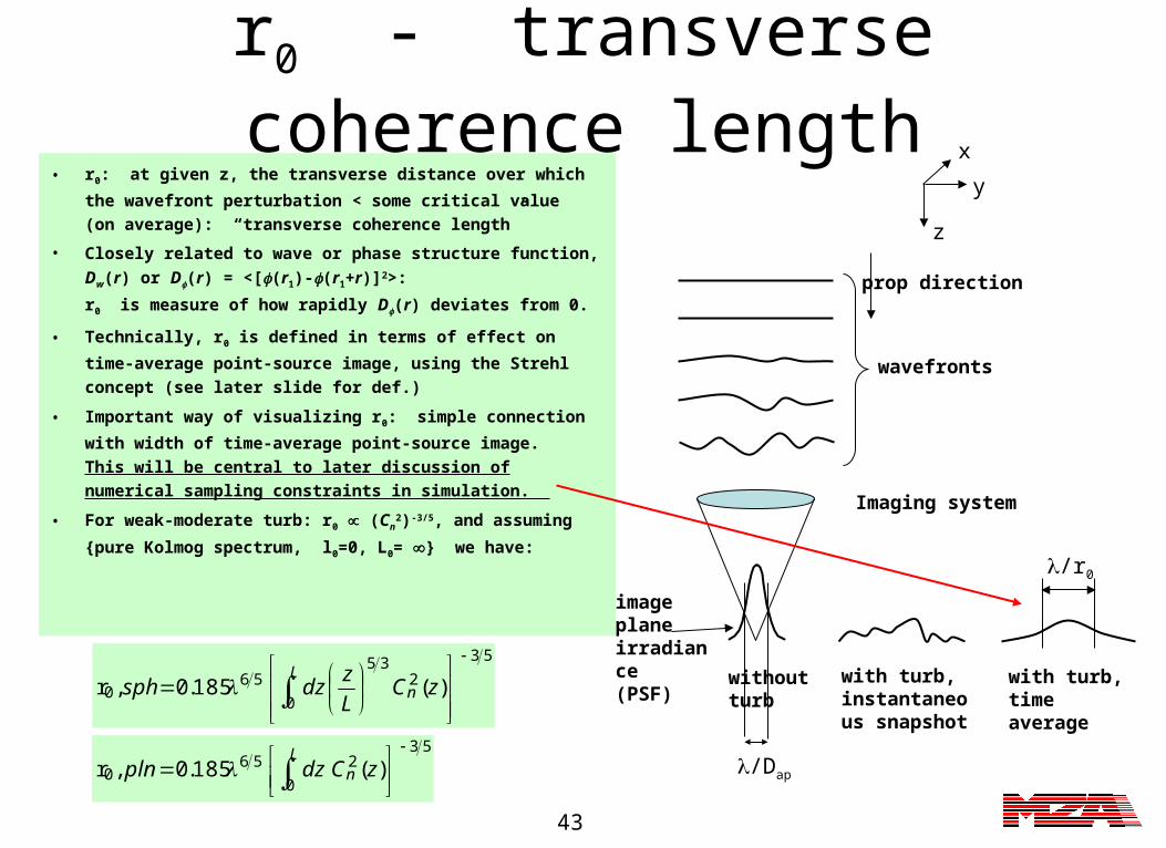
r0 - transverse coherence length

• r0: at given z, the transverse distance over which the

wavefront perturbation < some critical value (on

average): “transverse coherence length”

• Closely related to wave or phase structure function,

Dw(r) or D(r) = <[(r1)-(r1+r)]2>:

r0 is measure of how rapidly D(r) deviates from 0.

• Technically, r0 is defined in terms of effect on time-

average point-source image, using the Strehl

concept (see later slide for def.)

• Important way of visualizing r0: simple connection

with width of time-average point-source image.

This will be central to later discussion of numerical

sampling constraints in simulation.

• For weak-moderate turb: r0 (Cn2)-3/5, and assuming

{pure Kolmog spectrum, l0=0, L0= } we have:

prop direction

wavefronts

Imaging system


turbwith turb,instantaneous snapshot

with turb,time average

/r0

z

y

x

/Dap

53

0

235

560 )(185.0,r

Ln zC

L

zdzsph

53

0

2560 )(185.0,r

Ln zCdzpln

44

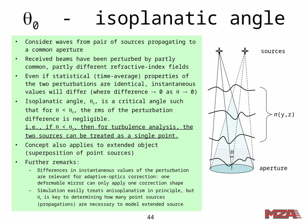
0 - isoplanatic angle• Consider waves from pair of sources propagating to a

common aperture

• Received beams have been perturbed by partly common, partly different refractive-index fields

• Even if statistical (time-average) properties of the two perturbations are identical, instantaneous values will differ (where difference 0 as 0)

• Isoplanatic angle, , is a critical angle such that for < , the

rms of the perturbation difference is negligible.

i.e., if < , then for turbulence analysis, the two sources can

be treated as a single point.

• Concept also applies to extended object (superposition of point sources)

• Further remarks:– Differences in instantaneous values of the perturbation are relevant for

adaptive-optics correction: one deformable mirror can only apply one correction shape

– Simulation easily treats anisoplanatism in principle, but is key to

determining how many point sources (propagations) are necessary to model extended source

n(y,z)

aperture

sources

45

Strehl ratio (SR)• SR is key optical-system performance parameter

in presence of aberrations (turbulence or static abs)

• Used for imaging as well as beam projection

• For small rms phase aberration in aperture (either intrinsically small or small because of adaptive correction), there are simple formulas relating SR to rms phase aberration.

• SR is correlated with spot width, but no unique relation exists because of different spot shape possibilities.

– Extension of concept: encircled-energy SR, or “bucket” SR.

– Used to comprehend spot width, or because useful energy is in some area around the peak.

• In field situations, Ino abs(0) can be difficult to

determine (because we can’t turn off turbulence). Computational formulas may be more elaborate than the given definition, but all are derived from that definition.

Imaging system


turbwith turb,instant. snapshot

with turb,time avg

/r0

/Dap

Ino abs(0): peak irrad in

image plane, if no aberrations present

I(0): peak irrad in image plane, with aberrations

)10(

)0(

)0(

SR

I

ISR

absno

46

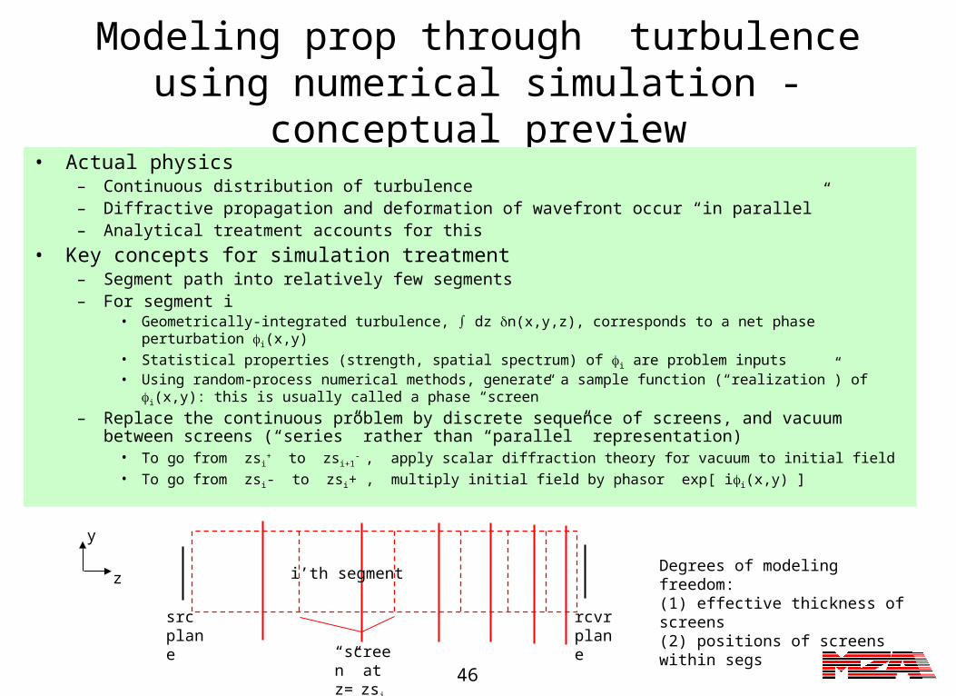
Modeling prop through turbulence using numerical simulation - conceptual preview

• Actual physics– Continuous distribution of turbulence – Diffractive propagation and deformation of wavefront occur “in parallel”– Analytical treatment accounts for this

• Key concepts for simulation treatment– Segment path into relatively few segments– For segment i

• Geometrically-integrated turbulence, dz n(x,y,z), corresponds to a net phase perturbation i(x,y)• Statistical properties (strength, spatial spectrum) of i are problem inputs• Using random-process numerical methods, generate a sample function (“realization”) of i(x,y): this is usually

called a phase “screen”

– Replace the continuous problem by discrete sequence of screens, and vacuum between screens (“series” rather than “parallel” representation)

• To go from zsi+ to zsi+1

- , apply scalar diffraction theory for vacuum to initial field• To go from zsi- to zsi+ , multiply initial field by phasor exp[ ii(x,y) ]

z

y

Degrees of modeling freedom:(1) effective thickness of screens(2) positions of screens within segs

src plane

rcvr plane

“screen” at z= zsi

i’th segment

47

Summary of key assumptions in treatment of turbulence

• Neglect polarization coupling by the turbulence• Spectrum used to construct phase screens is fundamentally Kolmogorov,

with possible addition of inner and outer scale• Temporal behavior dominated by frozen turbulence concept• For simulation work, replace parallel operation of turbulence and diffraction

by alternating model (propagate, apply screen, prop, apply screen, ...)

48

References for further study• R.E. Hufnagel, “Propagation through Atmospheric Turbulence”, Ch. 6 in

The Infrared Handbook, eds. Wolfe and Zissis, ERIM/ONR, rev. ed. 1985• R.R. Beland, “Propagation through Atmospheric Optical Turbulence”, Ch.

2 in Atmospheric Propagation of Radiation, vol. 2 of The Infrared and Electro-Optical Systems Handbook, ERIM and SPIE Press, 1993

• J. Goodman, “Imaging in the presence of randomly inhomogeneous media”, Ch. 8 in Statistical Optics, Wiley, 1985

• A. Ishimaru, Wave Propagation and Scattering in Random Media, IEEE Press/Oxford U. Press, reissue ed. 1997

• L.C. Andrews and R.L. Phillips, Laser Beam Propagation through Random Media, SPIE Press, 1998

• V.I. Tatarski, Wave Propagation in Turbulent Medium, McGraw-Hill, 1961• R.F. Lutomirski, R.E. Huschke, W.C. Meecham, and H.T. Yura,

Degradation of Laser Systems by Atmospheric Turbulence, DARPA Technical Report R-1171-ARPA/RC, June 1973

49

Special TopicsReflection from optically rough surfaces

Quasi-monochromatic light / temporal partial coherence

Polarization and birefringence, partial polarization

Thermal Blooming

Ultrashort pulses

Wide field incoherent imaging

…et cetera

We won’t have time to cover these topics in this workshop, but we’d be happy to discuss them off-line.

1 Modeling and Simulation of Beam Control Systems Part 1. Foundations of Wave Optics Simulation.

Documents

Transcript of 1 Modeling and Simulation of Beam Control Systems Part 1. Foundations of Wave Optics Simulation.