
1 Mining Closed & Maximal Frequent Itemsetscs.rpi.edu/~zaki/PaperDir/NGDMA05.pdf · ii MINING...
43
1 Mining Closed & Maximal Frequent Itemsets Mohammed J. Zaki † Computer Science Department Rensselaer Polytechnic Institute Troy NY 12180 USA Abstract In this chapter we give an overview of the closed and maximal itemset mining prob- lem. We survey existing methods and focus on Charm and GenMax, both state- of-the-art algorithms that efficiently enumerate all closed and maximal patterns, re- spectively. Charm and GenMax simultaneously explore both the itemset space and transaction space, and use a number of optimizations to quickly prune away a large portion of the subset search space. We conduct an extensive experimental charac- terization of GenMax and Charm against other maximal and closed pattern mining methods. We found that the methods have varying performance depending on the database characteristics (mainly the distribution of the closed or maximal frequent patterns by length). We present a systematic and realistic set of experiments showing under which conditions a method is likely to perform well and under what condi- tions it does not perform well. Overall, both Charm and GenMax deliver excellent † This work was supported in part by NSF CAREER Award IIS-0092978, DOE Early Career Award DE- FG02-02ER25538, NSF grant EIA-0103708 DRAFT November 16, 2003, 8:26pm DRAFT
Transcript of 1 Mining Closed & Maximal Frequent Itemsetscs.rpi.edu/~zaki/PaperDir/NGDMA05.pdf · ii MINING...

1 Mining Closed & MaximalFrequent Itemsets
Mohammed J. Zaki †
Computer Science Department
Rensselaer Polytechnic Institute
Troy NY 12180 USA
Abstract
In this chapter we give an overview of the closed and maximal itemset mining prob-
lem. We survey existing methods and focus on Charm and GenMax, both state-
of-the-art algorithms that efficiently enumerate all closed and maximal patterns, re-
spectively. Charm and GenMax simultaneously explore both the itemset space and
transaction space, and use a number of optimizations to quickly prune away a large
portion of the subset search space. We conduct an extensive experimental charac-
terization of GenMax and Charm against other maximal and closed pattern mining
methods. We found that the methods have varying performance depending on the
database characteristics (mainly the distribution of the closed or maximal frequent
patterns by length). We present a systematic and realistic set of experiments showing
under which conditions a method is likely to perform well and under what condi-
tions it does not perform well. Overall, both Charm and GenMax deliver excellent
†This work was supported in part by NSF CAREER Award IIS-0092978, DOE Early Career Award DE-
FG02-02ER25538, NSF grant EIA-0103708
D R A F T November 16, 2003, 8:26pm D R A F T
ii MINING CLOSED & MAXIMAL FREQUENT ITEMSETS
performance and outperform extant approaches for closed and maximal set mining.
However, there are a few exceptions to this, which we highlight in our experiments.
1.1 INTRODUCTION
Mining frequent itemsets is a fundamental and essential problem in many data min-
ing applications such as the discovery of association rules, strong rules, correlations,
multi-dimensional patterns, and many other important discovery tasks. The prob-
lem is formulated as follows: Given a large data base of set of items transactions,
find all frequent itemsets, where a frequent itemset is one that occurs in at least a
user-specified percentage of the data base.
Many of the proposed itemset mining algorithms are a variant of Apriori [2],
which employs a bottom-up, breadth-first search that enumerates every single fre-
quent itemset. In many applications (especially in dense data) with long frequent
patterns enumerating all possible 2m− 2 subsets of a m length pattern (m can easily
be 30 or 40 or longer) is computationally infeasible. For example, many real-world
domains like gene expression studies, network intrusion, web content and usage min-
ing, and so on, contain patterns are typically long. There are two current solutions to
the long pattern mining problem. The first solution one is to mine only the maximal
frequent itemsets [5, 12, 3, 6, 8]. A frequent set is maximal if it has no frequent
superset; the set of maximal patterns is typically orders of magnitude smaller than
all frequent patterns. While mining maximal sets help understand the long patterns
in dense domains, they lead to a loss of information; since subset frequency is not
available maximal sets are not suitable for generating rules. The second solution is
to mine only the frequent closed sets [4, 15, 14, 18, 21]; a frequent set is closed if
it has no superset with the same frequency. Closed sets are lossless in the sense that
they uniquely determine the set of all frequent itemsets and their exact frequency.
At the same time closed sets can themselves be orders of magnitude smaller than
all frequent sets, especially on dense databases. Nevertheless, for some of the dense
datasets we consider in this chapter, even the set of all closed patterns would grow to
be too large. The only recourse is to mine the maximal patterns in such domains.
D R A F T November 16, 2003, 8:26pm D R A F T

PRELIMINARIES iii
In this chapter we give an overview of the closed and maximal itemset mining
problem. We survey existing methods and focus on Charm and GenMax, both state-
of-the-art algorithms that efficiently enumerate all closed and maximal patterns, re-
spectively. Charm and GenMax simultaneously explore both the itemset space and
transaction space, and use a number of optimizations to quickly prune away a large
portion of the subset search space. GenMax uses a novel progressive focusing tech-
nique to eliminate non-maximal itemsets, while Charm uses a fast hash-based ap-
proach to eliminate non-closed itemsets during subsumption checking. Both utilize
diffset propagation for fast frequency checking. Diffsets [20] keep track of differ-
ences in the tids of a candidate pattern from its prefix pattern. Diffsets drastically
cut down (by orders of magnitude) the size of memory required to store intermediate
results. Thus the entire working set of patterns can fit entirely in main-memory, even
for large databases.
We conduct an extensive experimental characterization of GenMax against other
maximal pattern mining methods like MaxMiner [5] and Mafia [6]. We compare
Charm against previous methods for mining closed sets such as Close [14], Closet [15],
Mafia [6] and Pascal [4]. We found that the methods have varying performance
depending on the database characteristics (mainly the distribution of the closed or
maximal frequent patterns by length). We present a systematic and realistic set of
experiments showing under which conditions a method is likely to perform well and
under what conditions it does not perform well. Overall, both Charm and GenMax
deliver excellent performance and outperform extant approaches for closed and max-
imal set mining. However, there are a few exceptions to this, which we highlight in
our experiments.
1.2 PRELIMINARIES
The problem of mining closed and maximal frequent patterns can be formally stated
as follows: Let I = {i1, i2, . . . , im} be a set of m distinct items. Let D denote
a database of transactions, where each transaction has a unique identifier (tid) and
contains a set of items. The set of all tids is denoted T = {t1, t2, ..., tn}. A set
D R A F T November 16, 2003, 8:26pm D R A F T

iv MINING CLOSED & MAXIMAL FREQUENT ITEMSETS
X ⊆ I is also called an itemset. An itemset with k items is called a k-itemset. The
set t(X) ⊆ T , consisting of all the transaction tids which contain X as a subset, is
called the tidset of X . For convenience we write an itemset {A,C,W} as ACW ,
and its tidset {1, 3, 4, 5} as t(X) = 1345. For a tidset Y , we denote its corresponding
itemset as i(Y ), i.e., the set of items common to all the tids in Y . The composition of
the two functions, namely, t that maps from itemsets to tidsets, and i that maps from
tidsets to itemsets, is called a closure operator, and is given as c(X) = i(t(X)). For
instance c(AW ) = i(t(AW )) = i(1345) = ACW .
The support of an itemset X , denoted σ(X), is the number of transactions in
which that itemset occurs as a subset. Thus σ(X) = |t(X)|. An itemset is frequent
if its support is more than or equal to some threshold minimum support (min sup)
value, i.e., if σ(X) ≥ min sup. We denote by Fk the set of frequent k-itemsets, and
by FI the set of all frequent itemsets. A frequent itemset is called maximal if it is not
a subset of any other frequent itemset. The set of all maximal frequent itemsets is
denoted as MFI. A set is closed if it has no superset with the same frequency. The
set of all closed frequent itemsets is denoted as CFI. It can be shown that an itemset
X is closed if and only if c(X) = X [18]. Given a user specified min sup value our
goal is to efficiently enumerate all patterns in CFI and MFI.
[INSERT FIGURE 1.1 and 1.2 HERE]
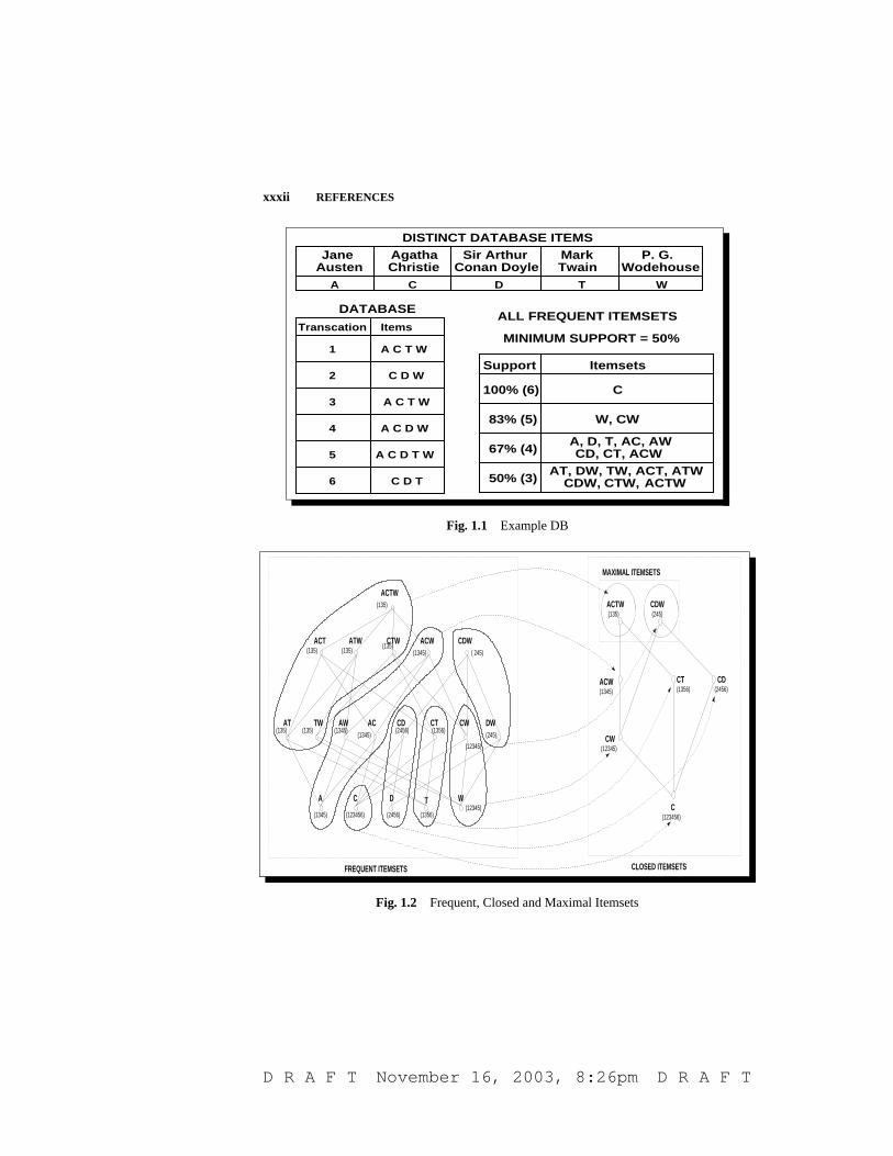
Example 1 Consider our example database in Figure 1.1. There are five different
items, I = {A,C,D, T,W} and six transactions T = {1, 2, 3, 4, 5, 6}. The table
on the right shows all 19 frequent itemsets for min sup= 3. The lattice for FI is
shown in Figure 1.2; under each itemset X , we show its tidset t(X). The figure also
shows the 7 closed sets obtained by collapsing all the itemsets that have the same
tidset (closed regions of the lattice), and the 2 maximal sets (circles). It is clear that
MFI ⊆ CFI ⊆ FI.
D R A F T November 16, 2003, 8:26pm D R A F T
PRELIMINARIES v
1.2.1 Backtracking Search
GenMax uses backtracking search to enumerate the MFI. We first describe the back-
tracking paradigm in the context of enumerating all frequent patterns. We will sub-
sequently modify this procedure to enumerate the MFI.
Backtracking algorithms are useful for many combinatorial problems where the
solution can be represented as a set I = {i0, i1, ...}, where each ij is chosen from
a finite possible set, Pj . Initially I is empty; it is extended one item at a time,
as the search space is traversed. The length of I is the same as the depth of the
corresponding node in the search tree. Given a partial solution of length l, Il =
{i0, i1, ..., il−1}, the possible values for the next item il comes from a subsetCl ⊆ Pl
called the combine set. If y ∈ Pl−Cl, then nodes in the subtree with root node Il =
{i0, i1, ..., il−1, y} will not be considered by the backtracking algorithm. Since such
subtrees have been pruned away from the original search space, the determination of
Cl is also called pruning.
[INSERT FIGURE 1.3 HERE ]
Consider the backtracking algorithm for mining all frequent patterns, shown in
Figure 1.3. The main loop tries extending Il with every item x in the current com-
bine set Cl. The first step is to compute Il+1, which is simply Il extended with x.
The second step is to extract the new possible set of extensions, Pl+1, which consists
only of items y in Cl that follow x. The third step is to create a new combine set for
the next pass, consisting of valid extensions. An extension is valid if the resulting
itemset is frequent. The combine set, Cl+1, thus consists of those items in the pos-
sible set that produce a frequent itemset when used to extend Il+1. Any item not in
the combine set refers to a pruned subtree. The final step is to recursively call the
backtrack routine for each extension. As presented, the backtrack method performs
a depth-first traversal of the search space.
[INSERT Figure 1.4 HERE ]
Example 2 Consider the full subset search space shown in Figure 1.4. The back-
track search space can be considerably smaller than the full space. For example, we
start with I0 = ∅ and C0 = F1 = {A,C,D, T,W}. At level 1, each item in C0 is
D R A F T November 16, 2003, 8:26pm D R A F T
vi MINING CLOSED & MAXIMAL FREQUENT ITEMSETS
added to I0 in turn. For example, A is added to obtain I1 = {A}. The possible set
for A, P1 = {C,D, T,W} consists of all items that follow A in C0. However, from
Figure 1.1, we find that only AC, AT , and AW are frequent (at min sup=3), giving
C1 = {C, T,W}. Thus the subtree corresponding to the node AD has been pruned.
1.3 EXISTING APPROACHES FOR CLOSED AND MAXIMAL ITEMSET
MINING
1.3.1 Maximal Itemset Mining
A good coverage of mining long patterns appears in [1]. Methods for finding the
maximal elements include All-MFS [10], which works by iteratively attempting to
extend a working pattern until failure. A randomized version of the algorithm that
uses vertical bit-vectors was studied, but it does not guarantee every maximal pattern
will be returned.
The Pincer-Search [12] algorithm uses horizontal data format. It not only con-
structs the candidates in a bottom-up manner like Apriori, but also starts a top-down
search at the same time, maintaining a candidate set of maximal patterns. This can
help in reducing the number of database scans, by eliminating non-maximal sets
early. The maximal candidate set is a superset of the maximal patterns, and in gen-
eral, the overhead of maintaining it can be very high. In contrast GenMax maintains
only the current known maximal patterns for pruning.
MaxMiner [5] is another algorithm for finding the maximal elements. It uses
efficient pruning techniques to quickly narrow the search. MaxMiner employs a
breadth-first traversal of the search space; it reduces database scanning by employing
a lookahead pruning strategy, i.e., if a node with all its extensions can determined to
be frequent, there is no need to further process that node. It also employs item
(re)ordering heuristic to increase the effectiveness of superset-frequency pruning.
Since MaxMiner uses the original horizontal database format, it can perform the
same number of passes over a database as Apriori does.
DepthProject [3] finds long itemsets using a depth first search of a lexicographic
tree of itemsets, and uses a counting method based on transaction projections along
D R A F T November 16, 2003, 8:26pm D R A F T

EXISTING APPROACHES FOR CLOSED AND MAXIMAL ITEMSET MINING vii
its branches. This projection is equivalent to a horizontal version of the tidsets at a
given node in the search tree. DepthProject also uses the look-ahead pruning method
with item reordering. It returns a superset of the MFI and would require post-pruning
to eliminate non-maximal patterns. FPgrowth [11] uses the novel frequent pattern
tree (FP-tree) structure, which is a compressed representation of all the transactions
in the database. It uses a recursive divide-and-conquer and database projection ap-
proach to mine long patterns. Nevertheless, since it enumerates all frequent patterns
it is impractical when pattern length is long.
Mafia [6] is the most recent method for mining the MFI. Mafia uses three pruning
strategies to remove non-maximal sets. The first is the look-ahead pruning first used
in MaxMiner. The second is to check if a new set is subsumed by an existing maximal
set. The last technique checks if t(X) ⊆ t(Y ). If so X is considered together
with Y for extension. Mafia uses vertical bit-vector data format, and compression
and projection of bitmaps to improve performance. Mafia mines a superset of the
MFI, and requires a post-pruning step to eliminate non-maximal patterns. In contrast
GenMax integrates pruning with mining and returns the exact MFI.
Among the most recent methods for MFI are SmartMiner [22] and FPMax [9].
SmartMiner doesn’t do explicit maximality checking; rather it uses the information
available from the previous combine sets to construct the new combine set at the
current node. It performs depth-first search and uses bitvector data representation.
FPMax mines maximal patterns from the FP-Tree data structure (am augmented pre-
fix tree) originally proposed in [11]. It also maintains the MFI in another prefix tree
data structure for maximality checking.
1.3.2 Closed Itemset Mining
There have been several recent algorithms proposed for mining CFI. Close [14] is
an Apriori-like algorithm that directly mines frequent closed itemsets. There are two
main steps in Close. The first is to use bottom-up search to identify generators, the
smallest frequent itemset that determines a closed itemset. For example, consider the
frequent itemset lattice in Figure 1.2. The item A is a generator for the closed set
ACW , since it is the smallest itemset with the same tidset as ACW . All generators
D R A F T November 16, 2003, 8:26pm D R A F T
viii MINING CLOSED & MAXIMAL FREQUENT ITEMSETS
are found using a simple modification of Apriori. After finding the frequent sets at
level k, Close compares the support of each set with its subsets at the previous level.
If the support of an itemset matches the support of any of its subsets, the itemset
cannot be a generator and is thus pruned. The second step in Close is to compute the
closed sets for all the generators found in the first step, which is done via intersection
of all transactions where it occurs as a subset. This can be done in one pass over the
database, provided all generators fit in memory. Nevertheless computing closures
this way is an expensive operation.
The authors of Close recently developed Pascal [4], an improved algorithm for
mining closed and frequent sets. They introduce the notion of key patterns and show
that other frequent patterns can be inferred from the key patterns without access
to the database. They showed that Pascal, even though it finds both frequent and
closed sets, is typically twice as fast as Close, and ten times as fast as Apriori. Since
Pascal enumerates all patterns, it is only practical when pattern length is short (as we
shall see in the experimental section). The Closure algorithm [7] is also based on
a bottom-up search; it performs only marginally better than Apriori. Charm uses a
more efficient depth-first search over itemset and tidsets spaces.
Closet [15] uses a novel frequent pattern tree (FP-tree) structure, which is a
compressed representation of all the transactions in the database. It uses a recur-
sive divide-and-conquer and database projection approach to mine long patterns.
Mafia [6] is primarily intended for maximal pattern mining, but has an option to
mine the closed sets as well. Mafia relies on efficient compressed and projected ver-
tical bitmap based frequency computation. In contrast to Closet and Mafia, Charm
uses diffsets for fast support computation.
Recently two new algorithms for finding frequent closed itemsets have been pro-
posed, Closet+ [16] and Carpenter [13]. Closet+ combines several previously pro-
posed as well as new effective strategies into one algorithm. Carpenter mines closed
patterns in datasets that have significantly more items than there are transactions,
such as datasets that arise in biology, for example, microarray datasets. In these
datasets, there can easily be 10,000 or more items, but only 100-1000 transactions.
All of the above algorithms for CFI cannot deal with such a large itemsets space
D R A F T November 16, 2003, 8:26pm D R A F T

EFFICIENT CFI AND MFI MINING: CHARM AND GENMAX ix
(e.g.,210000). Capitalizing on the fact that the tidset search space is much smaller
(e.g., 2100), Carpenter enumerates closed tidsets and determines the corresponding
closed itemsets from them.
1.4 EFFICIENT CFI AND MFI MINING: CHARM AND GENMAX
There are two main ingredients to develop an efficient CFI and MFI algorithm. The
first is the set of techniques used to remove entire branches of the search space, and
the second is the representation used to perform fast frequency computations. We
will describe below how Charm and GenMax extend the basic backtracking routine
for FI, and the progressive focusing, hash-based subsumption checking and diff-
set propagation techniques they use for fast maximality, closedness and frequency
checking. More details on Charm and GenMax, and on diffsets can be found in
[8, 21, 20].
1.4.1 Fast Frequency Testing
Typically, pattern mining algorithms use a horizontal database format, such as the
one shown in Figure 1.1, where each row is a tid followed by its itemset. Con-
sider a vertical database format, where for each item we list its tidset, the set of all
transaction tids where it occurs. The vertical representation has the following ma-
jor advantages over the horizontal layout: Firstly, computing the support of itemsets
is simpler and faster with the vertical layout since it involves only the intersections
of tidsets (or compressed bit-vectors if the vertical format is stored as bitmaps [6]).
Secondly, with the vertical layout, there is an automatic “reduction” of the database
before each scan in that only those itemsets that are relevant to the following scan
of the mining process are accessed from disk. Thirdly, the vertical format is more
versatile in supporting various search strategies, including breadth-first, depth-first
or some other hybrid search.
[INSERT Figure 1.5 HERE]
Let’s consider how the FI-combine (see Figure 1.3) routine works, where the
frequency of an extension is tested. Each item x in Cl actually represents the itemset
D R A F T November 16, 2003, 8:26pm D R A F T

x MINING CLOSED & MAXIMAL FREQUENT ITEMSETS
Il ∪ {x} and stores the associated tidset for the itemset Il ∪ {x}. For the initial
invocation, since Il is empty, the tidset for each item x in Cl is identical to the tidset,
t(x), of item x. Before line 3 is called in FI-combine, we intersect the tidset of the
element Il+1 (i.e., t(Il ∪ {x})) with the tidset of element y (i.e., t(Il ∪ {y})). If
the cardinality of the resulting intersection is above minimum support, the extension
with y is frequent, and y′ the new intersection result, is added to the combine set
Cl+1 for the next level. Cl+1 is kept in increasing order of support of its elements.
Figure 1.5 shows the pseudo-code for FI-tidset-combine using this tidset intersection
based support counting.
Example 3 Suppose, that we have the itemset ACT ; we show how to get its support
using the tidset intersections. We start with item A, and extend it with item C.
We find the support of AC as follows: t(AC) = t(A) ∩ t(C) = {1, 3, 4, 5} ∩{1, 2, 3, 4, 5} = {1, 3, 4, 5}, and the support of AC is then |t(AC)| = 4 At the
next level, we need to compute the tidset for ACT using the tidsets for AC and
AT , where Il = {A} and Cl = {C, T}. We have t(ACT ) = t(AC) ∩ t(AT ) =
{1, 3, 4, 5} − {1, 3, 5} = {1, 3, 5}, and its support is |t(ACT )| = 3.
1.4.1.1 Diffsets Propagation Despite the many advantages of the vertical format,
when the tidset cardinality gets very large (e.g., for very frequent items) the intersec-
tion time starts to become inordinately large. Furthermore, the size of intermediate
tidsets generated for frequent patterns can also become very large to fit into main
memory. Both Charm and GenMax uses a new format called diffsets [20] for fast
frequency testing.
The main idea of diffsets is to avoid storing the entire tidset of each element in
the combine set. Instead we keep track of only the differences between the tidset of
itemset Il and the tidset of an element x in the combine set (which actually denotes
Il ∪ {x}). These differences in tids are stored in what we call the diffset, which is a
difference of two tidsets at the root level or a difference of two diffsets at later levels.
Furthermore, these differences are propagated all the way from a node to its children
starting from the root. In an extensive study [20], we showed that diffsets are very
D R A F T November 16, 2003, 8:26pm D R A F T
EFFICIENT CFI AND MFI MINING: CHARM AND GENMAX xi
short compared to their tidsets counterparts, and are highly effective in improving
the running time of vertical methods.
[INSERT Figure 1.6 HERE]
We describe next how diffsets are used, with the help of an example. At level
0, we have available the tidsets for each item in F1. To find the combine set at this
level, we compute the diffset of y′, denoted as d(y′) instead of computing the tidset
of y as shown in line 4 in Figure 1.5. That is d(y′) = t(x) − t(y). The support of
y′ is now given as σ(y′) = σ(x) − |d(y′)|. At subsequent levels, we have available
the diffsets for each element in the combine list. In this case d(y′) = d(y) − d(x),
but the support is still given as σ(y′) = σ(x) − |d(y′)| [9]. Figure 1.6 shows the
pseudo-code for computing the combine sets using diffsets.
Example 4 Suppose, that we have the itemset ACT ; we show how to get its support
using the diffset propagation technique. We start with item A, and extend it with
item C. Now in order to find the support of AC we first find the diffset for AC,
denoted d(AC) = t(A)− t(C) = {1, 3, 4, 5} − {1, 2, 3, 4, 5} and then calculate its
support as σ(AC) = σ(A) − |d(AC)| = 4 − 0 = 4. At the next level, we need to
compute the diffset for ACT using the diffsets for AC and AT , where Il = {A} and
Cl = {C, T}. The diffset of itemsetACT is given as d(ACT ) = d(AT )−d(AC) =
{4} − {} = {4}, and its support is given as σ(AC)− |d(ACT )| = 4− 1 = 3.
1.4.2 Dynamically Reordering the Combine Set
Two general principles for efficient searching using backtracking are that: 1) It is
more efficient to make the next choice of a subtree (branch) to explore to be the one
whose combine set has the fewest items. This usually results in good performance,
since it minimizes the number of frequency computations in FI-combine. 2) If we
are able to remove a node as early as possible from the backtracking search tree we
effectively prune many branches from consideration.
Reordering the elements in the current combine set to achieve the two goals is
a very effective means of cutting down the search space. The first heuristic is to
reorder the combine set in increasing order of support. This is likely to produce
D R A F T November 16, 2003, 8:26pm D R A F T
xii MINING CLOSED & MAXIMAL FREQUENT ITEMSETS
small combine sets in the next level, since the items with lower frequency are less
likely to produce frequent itemsets at the next level. This heuristic was first used in
MaxMiner, and has been used in other methods since then [3, 6, 21]. At each level of
backtracking search, both Charm and GenMax reorder the combine set in increasing
order of support (this is indicated in Figures 1.3, 1.5, and 1.6).
1.4.3 Charm for CFI Mining
[INSERT Figure 1.7 HERE]
The FI-backtrack procedure can easily be extended to generate only closed sets,
as shown in Figure 1.7. Let Xi and Xj be two itemsets, we say that an itemset Xi
subsumes another itemset Xj , if and only if Xj ⊂ Xi and σ(Xj) = σ(Xi). Before
adding any frequent itemset X to CFI we need to make sure that it is not subsumed
(lines 6,7), i.e., there is no superset of X in CFI which has the same support, since
in that case X cannot be closed. There is no change in the rest of the enumeration
algorithm, however, this algorithm is inefficient, since it does subsumption checking
for each new itemset generated. There are two ways to optimize this: 1) reduce
the number of itemsets for which subsumption check is done, i.e., further prune the
backtrack search space, and 2) perform fast subsumption checking.
1.4.3.1 Pruning Search Space To prune the search space we can utilize certain
properties of itemset-diffset pairs as described in [21].
Theorem 1 ([21]) Let Xi = Il+1 ∪ {yi} and Xj = Il+1 ∪ {yj} be two members of
the possible set at level l, and let Xi× d(Xi) and Xj × d(Xj) be the corresponding
itemset-diffset pairs. The following four properties hold:
1. If d(Xi) = d(Xj), then c(Xi) = c(Xj) = c(Xi ∪Xj)
2. If d(Xi) ⊃ d(Xj), then c(Xi) 6= c(Xj), but c(Xi) = c(Xi ∪Xj)
3. If d(Xi) ⊂ d(Xj), then c(Xi) 6= c(Xj), but c(Xj) = c(Xi ∪Xj)
4. If d(Xi) 6= d(Xj), then c(Xi) 6= c(Xj) 6= c(Xi ∪Xj)
[INSERT Figure 1.8 HERE]
D R A F T November 16, 2003, 8:26pm D R A F T

EFFICIENT CFI AND MFI MINING: CHARM AND GENMAX xiii
Charm uses these four properties to prune the elements of the combine set, as
shown in Figure 1.8. CFI-diffset-combine is the same as FI-diffset-combine (in
Figure 1.6), except for lines 7-16 that are used to check the four properties outlined
in Theorem 1. According to Property 1, if the diffsets of y and Il+1 are identical
this means c(Il+1) = c(Il+1 ∪ {y}). In this case we prune the y branch of the
backtrack tree from further consideration (line 9) and replace Il+1 with Il+1 ∪ {y}(line 8). By Property 2, if d(y) ⊃ d(Il+1) then wherever Il+1 occurs y always co-
occurs, i.e., c(Il+1) = c(Il+1 ∪ {y}). We replace Il+1 with Il+1 ∪ {y} (line 11).
By Property 3 if d(y) ⊂ d(Il+1) then wherever y occurs Il+1 always co-occurs, i.e.,
c(y) = c(Il+1 ∪ {y}). We therefore remove the entire tree under y in Cl (line 14),
but we add y to Cl+1. Finally, if the diffsets of y and Il+1 are not equal, then no
pruning is possible; we add y to Cl+1.
Example 5 We explain the working of Charm using the example database in Fig-
ure 1.1. At the first level we have C0 = {A,C,D, T,W}, and thus within the for
loop in CFI-backtrack (Figure 1.7) we have I1 = A and P1 = {C,D, T,W}. We
next determine Cl+1 using CFI-diffset-combine. We find that t(A) ⊂ t(C) (Prop-
erty 2), i.e., whenever A occurs C co-occurs, thus we replace A with I1 = AC.
Considering the next element y = D, we find y′ = AD is not frequent. The next
item y = T yields a frequent itemset y′ = AT , but t(A) 6= t(T ), thus we set
C1 = {T}. Finally for y = W we again find t(A) ⊂ t(W ), thus we set I1 = ACW ,
and return C1 = {T}. In the next recursion ACWT will be found to be closed.
Next consider the second iteration of the for loop in CFI-backtrack. We have
I1 = C and P1 = {D,T,W}. In CFI-diffset-combine, we find that for all three
items Property 3 is true, i.e., whenever D,T,W occur, C always co-occurs, thus, we
prune them from the backtrack tree, and we get C0 = {A,C}, but C1 = {D,T,W},which will be recursively processed.
1.4.3.2 Fast Subsumption Checking In the CFI-backtrack method (Figure 1.7,
it may happen that after adding a closed set C to CFI, when we explore subsequent
branches of the backtrack tree, we may generate another set X , which cannot be
extended further, with X ⊆ C and with σ(C) = σ(X). In this case, X is a non-
D R A F T November 16, 2003, 8:26pm D R A F T

xiv MINING CLOSED & MAXIMAL FREQUENT ITEMSETS
closed set subsumed byC, and it should not be added to CFI. Since CFI dynamically
expands during enumeration of closed patterns, we need a very fast approach to
perform such subsumption checks.
Clearly we want to avoid comparing X with all existing elements in CFI, for this
would lead to a O(|CFI|2) complexity. To quickly retrieve relevant closed sets, the
obvious solution is to store CFI in a hash table. But what hash function to use?
Since we want to perform subset checking, we can’t hash on the itemset. We could
use the support of the itemsets for the hash function. But many unrelated itemsets
may have the same support. Since Charm uses diffsets/tidsets, it seems reasonable
to use the information from the tidsets to help identify if X is subsumed. Note that
if t(Xj) = t(Xi), then obviously σ(Xj) = σ(Xi). Thus to check if X is subsumed,
we can check if t(X) = t(C) for some C ∈ CFI. This check can be performed
in O(1) time using a hash table. But obviously we cannot afford to store the actual
tidset with each closed set in CFI; the space requirements would be prohibitive.
Charm adopts a compromise solution. It computes a hash function on the tidset
and stores in the hash table a closed set along with its support. Let h(Xi) denote
a suitable chosen hash function on the tidset t(Xi). Before adding X to CFI, we
retrieve from the hash table all entries with the hash key h(X). For each retrieved
closed set C, we then check if σ(X) = σ(C). If yes, we next check if X ⊂ C. If
yes, then X is subsumed and we do not add it to CFI.
What is a good hash function on a tidset? Charm uses the sum of the tids in
the tidset as the hash function, i.e., h(X) =∑
T∈t(X) T (note, this is not the same
as support, which is the cardinality of t(X)). We tried several other variations and
found there to be no performance difference. This hash function is likely to be as
good as any other due to several reasons. Firstly, by definition a closed set is one that
does not have a superset with the same support; it follows that it must have some tids
that do not appear in any other closed set. Thus the hash keys of different closed sets
will tend to be different. Secondly, even if there are several closed sets with the same
hash key, the support check we perform (i.e., if σ(X) = σ(C)) will eliminate many
closed sets whose keys are the same, but they in fact have different supports. Thirdly,
this hash function is easy to compute and it can easily be used with the diffset format.
D R A F T November 16, 2003, 8:26pm D R A F T
EFFICIENT CFI AND MFI MINING: CHARM AND GENMAX xv
1.4.4 GenMax for MFI Mining
[INSERT Figure 1.9 HERE ]
The basic MFI enumeration code used in GenMax is a straightforward exten-
sion of FI-backtrack. The main addition is the superset checking to eliminate non-
maximal itemsets, as shown in Figure 1.9. In addition to the main steps in FI enu-
meration, the new code adds a step (line 4) after the construction of the possible set
to check if Il+1∪Pl+1 is subsumed by an existing maximal set. If so, the current and
all subsequent items in Cl can be pruned away. After creating the new combine set,
if it is empty and Il+1 is not a subset of any maximal pattern, it is added to the MFI.
If the combine set is non-empty a recursive call is made to check further extensions.
Like Charm, GenMax makes use of properties of itemset-diffset pairs outlined in
Theorem 1; thus it uses the CFI-diffset-combine routine (line 6).
1.4.4.1 Superset Checking Techniques Checking to see if the given itemset Il+1
combined with the possible set Pl+1 is subsumed by another maximal set was also
proposed in Mafia [6] under the name HUTMFI. Further pruning is possible if one
can determine based just on support of the combine sets if Il+1 ∪ Pl+1 will be guar-
anteed to be frequent. In this case also one can avoid processing any more branches.
This method was first introduced in MaxMiner [5], and was also used in Mafia under
the name FHUT.
In addition to sorting the initial combine set at level 0 in increasing order of sup-
port, GenMax uses another reordering heuristic based on a simple lemma
Lemma 1 ([8]) Let IF (x) = {y : y ∈ F1, xy is not frequent }, denote the set of
infrequent 2-itemsets that contain an item x ∈ F1, and let M(x) be the longest
maximal pattern containing x. Then |M(x)| ≤ |F1| − |IF (x)|.
Assuming F2 has been computed, reordering C0 in decreasing order of IF (x)
(with x ∈ C0) ensures that the smallest combine sets will be processed at the initial
levels of the tree, which result in smaller backtracking search trees. GenMax thus
initially sorts the items in decreasing order of IF (x) and in increasing order of sup-
port. Then at each subsequent level, GenMax keeps the combine set in increasing
order of support as shown in Figure 1.6.
D R A F T November 16, 2003, 8:26pm D R A F T

xvi MINING CLOSED & MAXIMAL FREQUENT ITEMSETS
[INSERT FIGURE 1.10 HERE]
Example 6 For our database in Figure 1.1 with min sup = 2, IF (x) is the same of
all items x ∈ F1, and the sorted order (on support) is A,D, T,W,C. Figure 1.10
shows the backtracking search trees for maximal itemsets containing prefix items A
and D. Under the search tree for A, Figure 1.10 (a), we try to extend the partial
solution AD by adding to it item T from its combine set. We try another item W
after itemsetADT turns out to be infrequent, and so on. Since GenMax uses itemsets
which are found earlier in the search to prune the combine sets of later branches, after
finding the maximal set ADWC, GenMax skips ADC. After finding ATWC all
the remaining nodes with prefix A are pruned, and so on. The pruned branches are
shown with dashed arrows, indicating that a large part of the search tree is pruned
away
1.4.4.2 Superset Checking Optimization The main efficiency of GenMax stems
from the fact that it eliminates branches that are subsumed by an already mined
maximal pattern. Were it not for this pruning, GenMax would essentially default to
a depth-first exploration of the search tree. Before creating the combine set for the
next pass, in line 4 in Figure 1.9, GenMax check if Il+1 ∪ Pl+1 is contained within
a previously found maximal set. If yes, then the entire subtree rooted at Il+1 and
including the elements of the possible set are pruned. If no, then a new extension
is required. Another superset check is required at line 8, when Il+1 has no frequent
extension, i.e., when the combine set Cl+1 is empty. Even though Il+1 is a leaf node
with no extensions it may be subsumed by some maximal set, and this case is not
caught by the check in line 4 above.
The major challenge in the design of GenMax is how to perform this subset check-
ing in the current set of maximal patterns in an efficient manner. If we were to naively
implement and perform this search two times on an ever expanding set of maximal
patterns MFI, and during each recursive call of backtracking, we would be spending
a prohibitive amount of time just performing subset checks. Each search would take
O(|MFI|) time in the worst case, where MFI is the current, growing set of maximal
patterns. Note that some of the best algorithms for dynamic subset testing run in
D R A F T November 16, 2003, 8:26pm D R A F T

EFFICIENT CFI AND MFI MINING: CHARM AND GENMAX xvii
amortized time O(√s log s) per operation in a sequence of s operations [17] (for us
s = O(MFI)). In dense domain we have thousands to millions of maximal frequent
itemsets, and the number of subset checking operations performed would be at least
that much. Can we do better?
The answer is, yes! Firstly, we observe that the two subset checks (one on line 4
and the other on line 8) can be easily reduced to only one check. Since Il+1∪Pl+1 is
a superset of Il+1, in our implementation we do superset check only for Il+1∪Pl+1.
While testing this set, we store the maximum position, say p, at which an item in
Il+1 ∪ Pl+1 is not found in a maximal set M ∈ MFI. In other words, all items
before p are subsumed by some maximal set. For the superset test for Il+1, we check
if |Il+1| < p. If yes, Il+1 is non-maximal. If no, we add it to MFI.
The second observation is that performing superset checking during each recur-
sive call can be redundant. For example, suppose that the cardinality of the possible
set Pl+1 is m. Then potentially, MFI-backtrack makes m redundant subset checks,
if the current MFI has not changed during these m consecutive calls. To avoid such
redundancy, a simple check status flag is used. If the flag is false, no superset check
is performed. Before each recursive call the flag is false; it becomes true whenever
Cl+1 is empty, which indicates that we have reached a leaf, and have to backtrack.
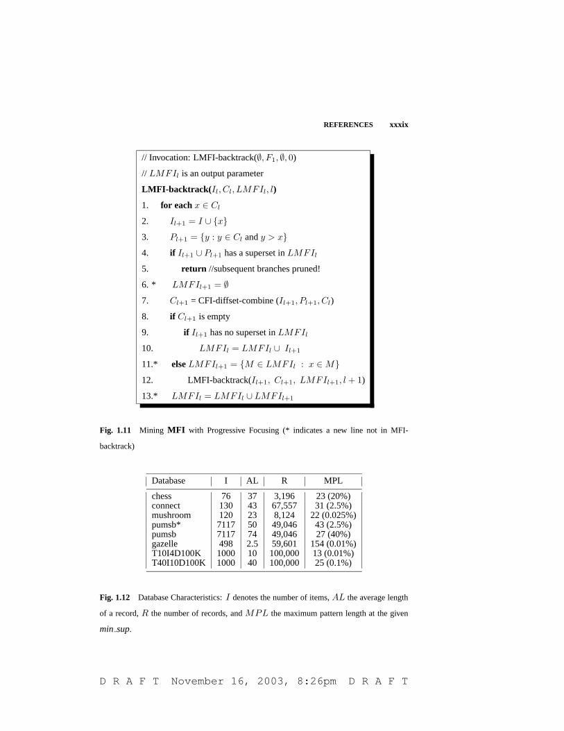
[INSERT Figure 1.11 HERE]
The O(√s log s) time bounds reported in [17] for dynamic subset testing do not
assume anything about the sequence of operations performed. In contrast, we have
full knowledge of how GenMax generates maximal sets; we use this observation to
substantially speed up the subset checking process. The main idea is to progressively
narrow down the maximal itemsets of interest as recursive calls are made. In other
words, we construct for each invocation of MFI-backtrack a list of local maximal
frequent itemsets, LMFIl. This list contains the maximal sets that can potentially
be supersets of candidates that are to be generated from the itemset Il. The only such
maximal sets are those that contain all items in Il. This way, instead of checking if
Il+1∪Pl+1 is contained in the full current MFI, we check only in LMFIl – the local
set of relevant maximal itemsets. This technique, that we call progressive focusing,
D R A F T November 16, 2003, 8:26pm D R A F T
xviii MINING CLOSED & MAXIMAL FREQUENT ITEMSETS
is extremely powerful in narrowing the search to only the most relevant maximal
itemsets, making superset checking practical on dense datasets.
Figure 1.11 shows the pseudo-code for GenMax that incorporates this optimiza-
tion (the code for the first two optimizations is not show to avoid clutter). Before
each invocation of LMFI-backtrack a new LMFIl+1 is created, consisting of those
maximal sets in the current LMFIl that contain the item x (see line 10). Any new
maximal itemsets from a recursive call are incorporated in the current LMFIl at line
12.
1.5 EXPERIMENTAL RESULTS
Past work has demonstrated that for MFI mining DepthProject [3] is faster than
MaxMiner [5], and the latest paper shows that Mafia [6] consistently beats DepthPro-
ject. In our experimental study below, we retain MaxMiner for baseline comparison.
At the same time, MaxMiner shows good performance on some datasets, which were
not used in previous studies. We use Mafia as the current state-of-the-art method and
show how GenMax compares against it. For comparison we used the original source
or object code for MaxMiner [5] and MAFIA [6], provided to us by their authors. For
CFI mining, we used the original source or object code for Close [14], Pascal [4],
Closet [15] and Mafia [6], all provided to us by their authors. We also include a
comparison with the base Apriori algorithm [2] for mining all itemsets.
All our experiments were performed on a 400MHz Pentium PC with 256MB of
memory, running RedHat Linux 6.0. Since Closet was provided as a Windows exe-
cutable by its authors, we compared it separately on a 900 MHz Pentium III processor
with 256MB memory, running Windows 98. Timings in the figures are based on total
wall-clock time, and include all preprocessing costs (such as horizontal-to-vertical
conversion in Charm, GenMax and Mafia). The times reported also include the pro-
gram output. We believe our setup reflects realistic testing conditions (as opposed
to some previous studies which report only the CPU time or may not include output
cost).
[INSERT Figure 1.12 HERE]
D R A F T November 16, 2003, 8:26pm D R A F T

EXPERIMENTAL RESULTS xix
1.5.1 Benchmark Datasets
We chose several real and synthetic datasets for testing the performance of the the
algorithms, shown in Table 1.12. The real datasets have been used previously in the
evaluation of maximal patterns [5, 3, 6]. Typically, these real datasets are very dense,
i.e., they produce many long frequent itemsets even for high values of support. The
table shows the length of the longest maximal pattern (at the lowest minimum sup-
port used in our experiments) for the different datasets. For example on pumsb*, the
longest pattern was of length 43 (any method that mines all frequent patterns will be
impractical for such long patterns). We also chose two synthetic datasets, which have
been used as benchmarks for testing methods that mine all frequent patterns. Previ-
ous maximal set mining algorithms have not been tested on these datasets, which are
sparser compared to the real sets. All these datasets are publicly available from IBM
Almaden (www.almaden.ibm.com/cs/quest/demos.html).
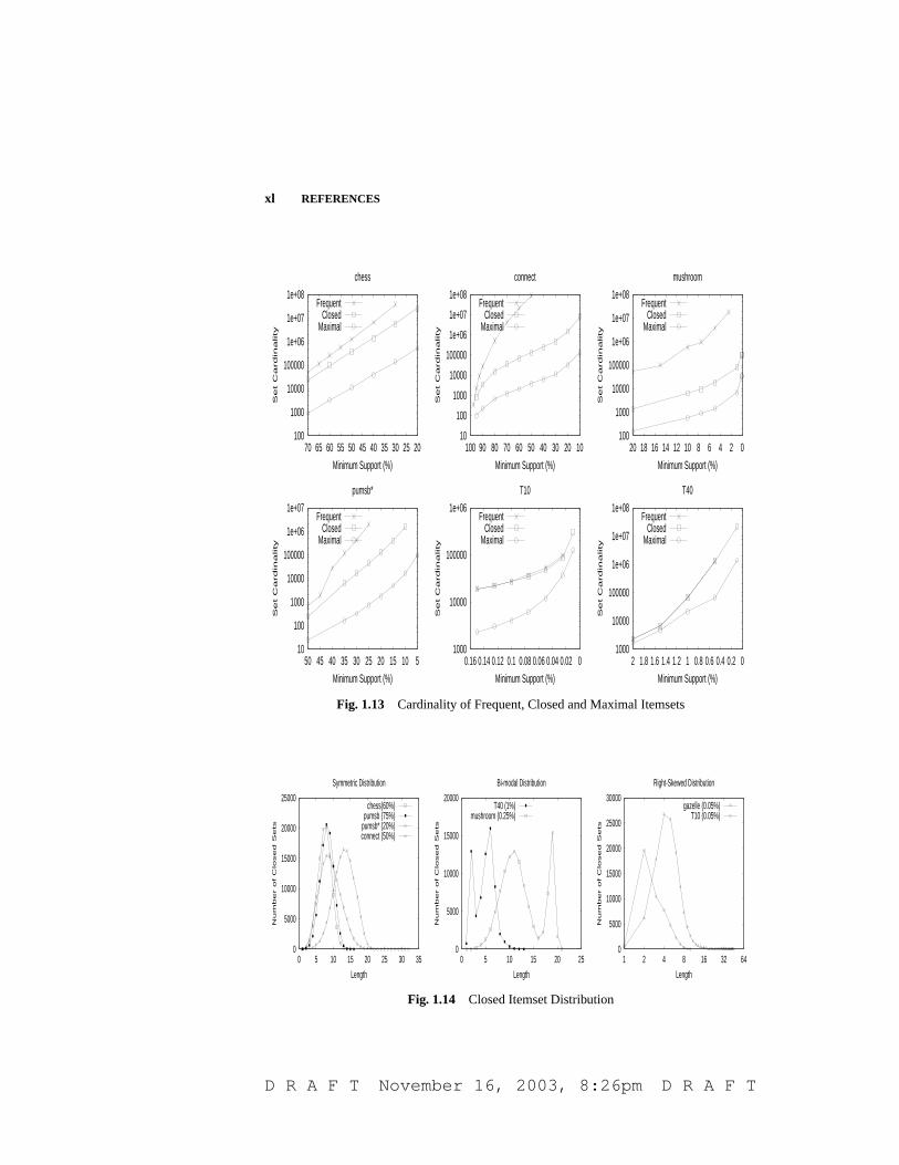
[INSERT Figure 1.13 HERE]
Figure 1.13 shows the total number of frequent, closed and maximal itemsets
found for various support values. The maximal frequent itemsets are a subset of the
frequent closed itemsets. The frequent closed itemsets are, of course, a subset of all
frequent itemsets. Depending on the support value used, for the real datasets, the set
of maximal itemsets is about an order of magnitude smaller than the set of closed
itemsets, which in turn is an order of magnitude smaller than the set of all frequent
itemsets. Even for very low support values we find that the difference between max-
imal and closed remains around a factor of 10. However the gap between closed and
all frequent itemsets grows more rapidly. Similar results were obtained for other real
datasets as well. On the other hand in sparse datasets the number of closed sets is
only marginally smaller than the number of frequent sets; the number of maximal
sets is still smaller, though the differences can narrow down for low support values.
[INSERT FIGURE 1.14 HERE ]
D R A F T November 16, 2003, 8:26pm D R A F T

xx MINING CLOSED & MAXIMAL FREQUENT ITEMSETS
1.5.2 Comparison of CFI Algorithms
Before we discuss the performance results of different algorithms it is instructive to
look at distribution of closed patterns by length for the various datasets, as shown
in Figure 1.14. We have grouped the datasets according to the type of distribution.
chess, pumsb*, pumsb, and connect all display an almost symmetric distribution of
the closed frequent patterns with different means. T40 and mushroom display an
interesting bi-modal distribution of closed sets. T40, like T10, has a many short
patterns of length 2, but it also has another peak at length 6. mushroom has consid-
erably longer patterns; its second peak occurs at 19. Finally gazelle and T10 have
a right-skewed distribution. gazelle tends to have many small patterns, with a very
long right tail. T10 exhibits a similar distribution, with the majority of the closed
patterns begin of length 2! The type of distribution tends to influence the behavior of
different algorithms as we will see below. The full comparison among the different
CFI algorithms is shown in Figure 1.15.
1.5.2.1 Type I: Symmetric Datasets Let us first compare how the methods per-
form on datasets which exhibit a symmetric distribution of closed itemsets, namely
chess, pumsb, connect and pumsb*. We observe that Apriori, Close and Pascal work
only for very high values of support on these datasets. The best among the three is
Pascal which can be twice as fast as Close, and up to 4 times better than Apriori. On
the other hand, Charm is several orders of magnitude better than Pascal, and it can
be run on very low support values, where none of the former three methods can be
run. Comparing with Mafia, we find that both Charm and Mafia have similar per-
formance for higher support values. However, as we lower the minimum support,
the performance gap between Charm and Mafia widens. For example at the lowest
support value plotted, Charm is about 30 times faster than Mafia on Chess, about 3
times faster on connect and pumsb, and 4 times faster on pumsb*. Charm outper-
forms Closet by an order of magnitude or more, especially as support is lowered. On
chess and pumsb* it is about 10 times faster than Closet, and about 40 times faster on
pumsb. On connect Closet performs better at high supports, but Charm does better
at lower supports. The reason is that connect has transactions with lot of overlap
D R A F T November 16, 2003, 8:26pm D R A F T

EXPERIMENTAL RESULTS xxi
among items, leading to a compact FP-tree and to faster performance. However, as
support is lowered FP-tree starts to grow, and Closet loses its edge.
[ INSERT FIGURE 1.15 HERE ]
1.5.2.2 Type II: Bi-modal Datasets On the two datasets with a bi-modal distri-
bution of frequent closed patterns, namely mushroom and T40, we find that Pascal
fares better than for symmetric distributions. For higher values of support the maxi-
mum closed pattern length is relatively short, and the distribution is dominated by the
first mode. Apriori, Close and Pascal can hand this case. However, as one lowers the
minimum support the second mode starts to dominate, with longer patterns. These
these methods thus quickly lose steam and become uncompetitive. Between Charm
and Mafia, up to 1% minimum support there is negligible difference, however, when
the support is lowered there is a huge difference in performance. Charm is about 20
times faster on mushroom and 10 times faster on T40 for the lowest support shown.
The gap continues to widen sharply. We find that Charm outperforms Closet by a
factor of 2 for mushroom and 4 for T40.
1.5.2.3 Type III: Right-Skewed Datasets On gazelle and T10, which have a large
number of very short closed patterns, followed by a sharp drop, we find that Apriori,
Close and Pascal remain competitive even for relatively low supports. The reason
is that T10 had a maximum pattern length of 11 at the lowest support shown. Also
gazelle at 0.06% support also had a maximum pattern length of 11. The level-wise
search of these three methods is able to easily handle such short patterns. However,
for gazelle, we found that at 0.05% support the maximum pattern length suddenly
jumped to 45, and none of these three methods could be run.
T10, though a sparse dataset, is problematic for Mafia. The reason is that T10
produces long sparse bitvectors for each item, and offers little scope for bit-vector
compression and projection that Mafia relies on for efficiency. This causes Mafia
to be uncompetitive for such datasets. Similarly Mafia fails to do well on gazelle.
However, it is able to run on the lowest support value. The diffset format of Charm is
resilient to sparsity (as shown in [20]) and it continues to outperform other methods.
For the lowest support, on T10 it is twice as fast as Pascal and 15 times better than
D R A F T November 16, 2003, 8:26pm D R A F T

xxii MINING CLOSED & MAXIMAL FREQUENT ITEMSETS
Mafia, and it is about 70 times faster than Mafia on gazelle. Charm is about 2 times
slower than Closet on T10. The reason is that the majority of closed sets are of length
2, and the tidset/diffsets operations in Charm are relatively expensive compared to
the compact FP-tree for short patterns (max length is only 11). However, for gazelle,
which has much longer closed patterns, Charm outperforms Closet by a factor of
160!
1.5.3 Comparison of MFI Algorithms
While conducting experiments comparing the 3 different algorithms, we observed
that the performance can vary significantly depending on the dataset characteristics.
We were able to classify our benchmark datasets into four classes based on the dis-
tribution of the maximal frequent patterns.
[INSERT Figure 1.16 HERE ]
1.5.3.1 Type I Datasets: Chess and Pumsb Figure 1.16 shows the performance
of the three algorithms on chess and pumsb. These Type I datasets are character-
ized by a symmetric distribution of the maximal frequent patterns (leftmost graph).
Looking at the mean of the curve, we can observe that for these datasets most of the
maximal patterns are relatively short (average length 11 for chess and 10 for pumsb).
The MFI cardinalities in Figure 1.13 show that for the support values shown, the
MFI is 2 orders of magnitude smaller than all frequent itemsets.
Compare the total execution time for the different algorithms on these datasets
(center and rightmost graphs). We use two different variants of Mafia. The first
one, labeled Mafia, does not return the exact maximal frequent set, rather it returns
a superset of all maximal patterns. The second variant, labeled MafiaPP, uses an
option to eliminate non-maximal sets in a post-processing (PP) step. Both GenMax
and MaxMiner return the exact MFI.
On chess we find that Mafia (without PP) is the fastest if one is willing to live
with a superset of the MFI. Mafia is about 10 times faster than MaxMiner. However,
notice how the running time of MafiaPP grows if one tries to find the exact MFI in
a post-pruning step. GenMax, though slower than Mafia is significantly faster than
D R A F T November 16, 2003, 8:26pm D R A F T

EXPERIMENTAL RESULTS xxiii
MafiaPP and is about 5 times better than MaxMiner. All methods, except MafiaPP,
show an exponential growth in running time (since the y-axis is in log-scale, this
appears linear) faithfully following the growth of MFI with lowering minimum sup-
port, as shown in the top center and right figures. MafiaPP shows super-exponential
growth and suffers from an approximately O(|MFI|2) overhead in pruning non-
maximal sets and thus becomes impractical when MFI becomes too large, i.e., at
low supports.
On pumsb, we find that GenMax is the fastest, having a slight edge over Mafia.
It is about 2 times faster than MafiaPP. We observed that the post-pruning routine in
MafiaPP works well till around O(104) maximal itemsets. Since at 60% min sup we
had around that many sets, the overhead of post-processing was not significant. With
lower support the post-pruning cost becomes significant, so much so that we could
not run MafiaPP beyond 50% minimum support. MaxMiner is significantly slower
on pumsb; a factor of 10 times slower then both GenMax and Mafia.
Type I results substantiate the claim that GenMax is an highly efficient method
to mine the exact MFI. It is as fast as Mafia on pumsb and within a factor of 2 on
chess. Mafia, on the other hand is very effective in mining a superset of the MFI.
Post-pruning, in general, is not a good idea, and GenMax beats MafiaPP with a wide
margin (over 100 times better in some cases, e.g., chess at 20%). On Type I data
MaxMiner is noncompetitive.
[INSERT FIGURE 1.17 HERE ]
1.5.3.2 Type II Datasets: Connect and Pumsb* Type II datasets, as shown in
Figure 1.17 are characterized by a left-skewed distribution of the maximal frequent
patterns, i.e., there is a relatively gradual increase with a sharp drop in the number of
maximal patterns. The mean pattern length is also longer than in Type I datasets; it
is around 16 or 17. The MFI cardinality (Figure 1.13) is also drastically smaller than
FI cardinality; by a factor of 104 or more (in contrast, for Type I data, the reduction
was only 102).
The main performance trend for both Type II datasets is that Mafia is the best
till the support is very low, at which point there is a cross-over and GenMax outper-
D R A F T November 16, 2003, 8:26pm D R A F T

xxiv MINING CLOSED & MAXIMAL FREQUENT ITEMSETS
forms Mafia. MafiaPP continues to be favorable for higher supports, but once again
beyond a point post-pruning costs start to dominate. MafiaPP could not be run be-
yond the plotted points. MaxMiner remains noncompetitive (about 10 times slower).
The initial start-up time for Mafia for creating the bit-vectors is responsible for the
high offset at 50% support on pumsb*. GenMax appears to exhibit a more graceful
increase in running time than Mafia.
[INSERT Figure 1.18 HERE ]
1.5.3.3 Type III Datasets: T10I4 and T40I10 As depicted in Figure 1.18, Type
III datasets – the two synthetic ones – are characterized by an exponentially decaying
distribution of the maximal frequent patterns. Except for a few maximal sets of size
one, the vast majority of maximal patterns are of length two! After that the number of
longer patterns drops exponentially. The mean pattern length is very short compared
to Type I or Type II datasets; it is around 4-6. MFI cardinality is not much smaller
than the cardinality of all frequent patterns (see Figure 1.13). The difference is only
a factor of 10 compared to a factor of 100 for Type I and a factor of 10,000 for Type
II.
Comparing the running times we observe that MaxMiner is the best method for
this type of data. The breadth-first or level-wise search strategy used in MaxMiner
is ideal for very bushy search trees, and when the average maximal pattern length
is small. Horizontal methods are better equipped to cope with the quadratic blowup
in the number of frequent 2-itemsets since one can use array based counting to get
their frequency. On the other hand vertical methods spend much time in performing
intersections on long item tidsets or bit-vectors. GenMax gets around this problem
by using the horizontal format for computing frequent 2-itemsets (denoted F2), but
it still has to spend time performing O(|F2|) pairwise tidset intersections.
Mafia on the other hand performs O(|F1|2) intersections, where F1 is the set of
frequent items. The overhead cost is enough to render Mafia noncompetitive on Type
III data. On T10 Mafia can be 20 or more times slower than MaxMiner. GenMax
exhibits relatively good performance, and it is about 10 times better than Mafia and
2 to 3 times worse than MaxMiner. On T40, the gap between GenMax/Mafia and
D R A F T November 16, 2003, 8:26pm D R A F T

CONCLUSIONS xxv
MaxMiner is smaller since there are longer maximal patterns. MaxMiner is 2 times
better than GenMax and 5 times better than Mafia. Since the MFI cardinality is
not too large MafiaPP has almost the time as Mafia for high supports. Once again
MafiaPP could not be run for lower support values. It is clear that, in general, post-
pruning is not a good idea; the overhead is too much to cope with.
[INSERT Figure 1.19 HERE ]
1.5.3.4 Type IV Dataset: Mushroom Mushroom exhibits a very unique MFI
distribution. Plotting MFI cardinality by length, we observe in Figure 1.19 that the
number of maximal patterns remains small until length 19. Then there is a sudden
explosion of maximal patterns at length 20, followed by another sharp drop at length
21. The vast majority of maximal itemsets are of length 20. The average transaction
length for mushroom is 23 (see Table 1.12), thus a maximal pattern spans almost
a full transaction. The total MFI cardinality is about 1000 times smaller than all
frequent itemsets (see Figure 1.13).
On Type IV data, Mafia performs the best. MafiaPP and MaxMiner are compa-
rable at lower supports. This data is the worst for GenMax, which is 2 times slower
than MaxMiner and 4 times slower than Mafia. In Type IV data, a smaller itemset
is part of many maximal itemsets (of length 20 in case of mushroom); this renders
our progressive focusing technique less effective. To perform maximality check-
ing one has to test against a large set of maximal itemsets; we found that GenMax
spends half its time in maximality checking. Recognizing this helped us improve
the progressive focusing using an optimized intersection-based method (as opposed
to the original list based approach). This variant, labeled GenMax’, was able to cut
down the execution time by half. GenMax’ runs in the same time as MaxMiner and
MafiaPP.
1.6 CONCLUSIONS
This is one of the first works to comprehensively compare recent closed and maximal
pattern mining algorithms under realistic assumptions. Our timings are based on
D R A F T November 16, 2003, 8:26pm D R A F T
xxvi MINING CLOSED & MAXIMAL FREQUENT ITEMSETS
wall-clock time, we included all pre-processing costs, and also cost of outputting all
the closed and maximal itemsets (written to a file). We were able to distinguish three
different types of CFI distributions and four different types of MFI distributions in
our benchmark testbed. We believe these distributions to be fairly representative of
what one might see in practice, since they span both real and synthetic datasets. For
CFI mining, Type I is a symmetric/normal CFI distribution, with both small and
long mean pattern lengths, Type II is a bi-modal distributions with both long and
short modes, and Type III is a right-skewed distribution with relatively short closed
pattern lengths. For MFI mining, Type I is a normal MFI distribution with not too
long maximal patterns, Type II is a left-skewed distributions, with longer maximal
patterns, Type III is an exponential decay distribution, with extremely short maximal
patterns, and finally Type IV is an extreme left-skewed distribution, with very large
average maximal pattern length.
We noted that different algorithms perform well under different distributions.
Among the CFI mining algorithms Charm performs the best for all distribution
types, with the exception of T10 dataset that is sparse and has very short pattern
lengths. For connect and mushroom Closet does better for high support values, but
Charm outperforms at lower supports. Mafia was not found to be competitive with
Charm, and neither were Pascal or Close. Among the current methods for MFI min-
ing, MaxMiner is the best for mining Type III distributions. On the remaining types,
Mafia is the best method if one is satisfied with a superset of the MFI. For very low
supports on Type II data, Mafia loses its edge. Post-pruning non-maximal patterns
typically has high overhead. It works only for high support values, and MafiaPP can-
not be run beyond a certain minimum support value. GenMax integrates pruning of
non-maximal itemsets in the process of mining using the novel progressive focusing
technique, along with other optimizations for superset checking; GenMax is the best
method for mining the exact MFI.
D R A F T November 16, 2003, 8:26pm D R A F T
CONCLUSIONS xxvii
Acknowledgments
We would like to thank Roberto Bayardo for providing us the MaxMiner algorithm; Lotfi
Lakhal and Yves Bastide for providing us the source code for Close and Pascal; Jiawei Han,
Jian Pei, and Jianyong Wang for sending us the executable for Closet; and Johannes Gehrke
for the Mafia algorithm. We thanks Roberto Bayardo for providing us the IBM real datasets,
and Ronny Kohavi and Zijian Zheng of Blue Martini Software for giving us access to the
Gazelle dataset.
D R A F T November 16, 2003, 8:26pm D R A F T


References
1. C. Aggarwal. Towards long pattern generation in dense databases. SIGKDD
Explorations, 3(1):20–26, 2001.
2. R. Agrawal, H. Mannila, R. Srikant, H. Toivonen, and A. Inkeri Verkamo. Fast
discovery of association rules. In U. Fayyad and et al, editors, Advances in
Knowledge Discovery and Data Mining, pages 307–328. AAAI Press, Menlo
Park, CA, 1996.
3. Ramesh Agrawal, Charu Aggarwal, and V.V.V. Prasad. Depth First Generation
of Long Patterns. In 7th Int’l Conference on Knowledge Discovery and Data
Mining, August 2000.
4. Y. Bastide, R. Taouil, N. Pasquier, G. Stumme, and L. Lakhal. Mining frequent
patterns with counting inference. SIGKDD Explorations, 2(2), December 2000.
5. R. J. Bayardo. Efficiently mining long patterns from databases. In ACM SIG-
MOD Conf. Management of Data, June 1998.
6. D. Burdick, M. Calimlim, and J. Gehrke. MAFIA: a maximal frequent itemset
algorithm for transactional databases. In Intl. Conf. on Data Engineering, April
2001.
7. D. Cristofor, L. Cristofor, and D. Simovici. Galois connection and data mining.
Journal of Universal Computer Science, 6(1):60–73, 2000.
8. K. Gouda and M. J. Zaki. Efficiently mining maximal frequent itemsets. In 1st
IEEE Int’l Conf. on Data Mining, November 2001.
D R A F T November 16, 2003, 8:26pm D R A F T

xxx REFERENCES
9. G. Grahne and J. Zhu. High performance mining of maximal frequent itemsets.
In 6th International Workshop on High Performance Data Mining, May 2003.
10. D. Gunopulos, H. Mannila, and S. Saluja. Discovering all the most specific
sentences by randomized algorithms. In Intl. Conf. on Database Theory, January
1997.
11. J. Han, J. Pei, and Y. Yin. Mining frequent patterns without candidate generation.
In ACM SIGMOD Conf. Management of Data, May 2000.
12. D-I. Lin and Z. M. Kedem. Pincer-search: A new algorithm for discovering
the maximum frequent set. In 6th Intl. Conf. Extending Database Technology,
March 1998.
13. F. Pan, G. Cong, A.K.H. Tung, J. Yang, and M.J. Zaki. CARPENTER: Finding
closed patterns in long biological datasets. In ACM SIGKDD Int’l Conf. on
Knowledge Discovery and Data Mining, August 2003.
14. N. Pasquier, Y. Bastide, R. Taouil, and L. Lakhal. Discovering frequent closed
itemsets for association rules. In 7th Intl. Conf. on Database Theory, January
1999.
15. J. Pei, J. Han, and R. Mao. Closet: An efficient algorithm for mining frequent
closed itemsets. In SIGMOD Int’l Workshop on Data Mining and Knowledge
Discovery, May 2000.
16. J. Wang, J. Han, and J. Pei. Closet+: Searching for the best strategies for mining
frequent closed itemsets. In ACM SIGKDD Int’l Conf. on Knowledge Discovery
and Data Mining, August 2003.
17. D.M. Yellin. An algorithm for dynamic subset and intersection testing. Theo-
retical Computer Science, 129:397–406, 1994.
18. M. J. Zaki. Generating non-redundant association rules. In 6th ACM SIGKDD
Int’l Conf. Knowledge Discovery and Data Mining, August 2000.
D R A F T November 16, 2003, 8:26pm D R A F T
REFERENCES xxxi
19. M. J. Zaki. Scalable algorithms for association mining. IEEE Transactions on
Knowledge and Data Engineering, 12(3):372-390, May-June 2000.
20. M. J. Zaki and K. Gouda. Fast vertical mining using Diffsets. Technical report,
9th ACM SIGKDD Int’l Conf. Knowledge Discovery and Data Mining, August
2003.
21. M. J. Zaki and C.-J. Hsiao. CHARM: An efficient algorithm for closed itemset
mining. In 2nd SIAM International Conference on Data Mining, April 2002.
22. Q. Zou, W.W. Chu, and B. Lu. Smartminer: a depth first algorithm guided by
tail information for mining maximal frequent itemsets. In 2nd IEEE Int’l Conf.
on Data Mining, November 2002.
D R A F T November 16, 2003, 8:26pm D R A F T
xxxii REFERENCES
C D T
A C D T W
A C D W
A C T W
C D W
A C T W
A C D T W
6
5
3
4
2
1
DATABASE
MINIMUM SUPPORT = 50%
ALL FREQUENT ITEMSETS
C
W, CW
A, D, T, AC, AWCD, CT, ACW
100% (6)
83% (5)
67% (4)
50% (3)AT, DW, TW, ACT, ATW
ItemsetsSupport
CTW,CDW, ACTW
ItemsTranscation
JaneAusten
AgathaChristie
Sir ArthurDISTINCT DATABASE ITEMS
Conan DoyleP. G.
WodehouseMarkTwain
Fig. 1.1 Example DB
DWTW AWAT AC CD CT CW
CDWACWCTWATWACT
ACTW
CW
ACW
ACTW CDW
CDCT
(1345) (123456)
(135)
(1345) (2456)
(135) (135)
(135)
(135) (135)
(1345)
(1345)
(2456) (1356)
(1356)
(12345)
(12345)
(245)
( 245)
(123456)
(2456)(1356)(1345)
(12345)
(245)(135)
A DC T WC
MAXIMAL ITEMSETS
CLOSED ITEMSETSFREQUENT ITEMSETS
Fig. 1.2 Frequent, Closed and Maximal Itemsets
D R A F T November 16, 2003, 8:26pm D R A F T
REFERENCES xxxiii
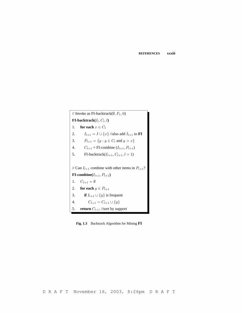
// Invoke as FI-backtrack(∅, F1, 0)
FI-backtrack(Il, Cl, l)
1. for each x ∈ Cl
2. Il+1 = I ∪ {x} //also add Il+1 to FI
3. Pl+1 = {y : y ∈ Cl and y > x}4. Cl+1 = FI-combine (Il+1, Pl+1)
5. FI-backtrack(Il+1, Cl+1, l + 1)
// Can Il+1 combine with other items in Pl+1?
FI-combine(Il+1, Pl+1)
1. Cl+1 = ∅2. for each y ∈ Pl+1
3. if Il+1 ∪ {y} is frequent
4. Cl+1 = Cl+1 ∪ {y}5. return Cl+1 //sort by support
Fig. 1.3 Backtrack Algorithm for Mining FI
D R A F T November 16, 2003, 8:26pm D R A F T

xxxiv REFERENCES
A{C,T,W}
AC{T,W} AD{T,W} AT{W} AW
ACD{T,W} ACT{W} ACW
ACDT{W} ACDW ACTW
ADT ADW ATW
C{D,T,W}
CD{T,W} CT{W} CW
CDT{W}
CDTW
CDW
DT{W} DW TW
CTW DTW
D{TW} T{W} W
{}{A,C,D,T,W}
ADTW
ACDTW
Level
0
1
2
3
4
5
Fig. 1.4 Subset/Backtrack Search Tree (min sup= 3): Circles indicate maximal sets and the
infrequent sets have been crossed out. Due to the downward closure property of support (i.e.,
all subsets of a frequent itemset must be frequent) the frequent itemsets form a border (shown
with the bold line), such that all frequent itemsets lie above the border, while all infrequent
itemsets lie below it. Since MFI determine the border, it is straightforward to obtain FI in a
single database scan if MFI is known.
D R A F T November 16, 2003, 8:26pm D R A F T

REFERENCES xxxv
// Can Il+1 combine with other items in Pl+1?
FI-tidset-combine(Il+1, Pl+1)
1. Cl+1 = ∅2. for each y ∈ Pl+1
3.* y′ = y
4.* t(y′) = t(Il+1) ∩ t(y)5.* if |t(y′)| ≥ min sup
6. Cl+1 = Cl+1 ∪ {y′}7. Sort Cl+1 by increasing support
8. return Cl+1
Fig. 1.5 FI-combine Using Tidset Intersections (* indicates a new line not in FI-combine)
// Can Il+1 combine with other items in Cl?
FI-diffset-combine(Il+1, Pl+1)
1. Cl+1 = ∅2. for each y ∈ Pl+1
3. y′ = y
4.* if level == 0 then d(y′) = t(Il+1)− t(y)
5.* else d(y′) = d(y)− d(Il+1)
6. if σ(y′) ≥ min sup
7. Cl+1 = Cl+1 ∪ {y′}8. Sort Cl+1 by increasing support
9. return Cl+1
Fig. 1.6 FI-combine using Diffsets (* indicates a new line not in FI-tidset-combine)
D R A F T November 16, 2003, 8:26pm D R A F T

xxxvi REFERENCES
// Invocation: CFI-backtrack(∅, F1, 0)
CFI-backtrack(Il, Cl, l)
1. for each x ∈ Cl
2. Il+1 = I ∪ {x} //also add Il+1 to FI
3. Pl+1 = {y : y ∈ Cl and y > x}4. Cl+1 = FI-diffset-combine (Il+1, Pl+1, Cl)
5. CFI-backtrack(Il+1, Cl+1, l + 1)
6.* if Il+1 has no superset in CFI with same support
7.* CFI= CFI ∪ Il+1
Fig. 1.7 Backtrack Algorithm for Mining CFI (* indicates a new line not in FI-backtrack)
D R A F T November 16, 2003, 8:26pm D R A F T

REFERENCES xxxvii
//Return Cl+1; can modify Cl also CFI-diffset-combine(Il+1, Pl+1, Cl)
1. Cl+1 = ∅2. for each y ∈ Pl+1
3. y′ = y
4. if level == 0 then d(y′) = t(Il+1)− t(y)
5. else d(y′) = d(y)− d(Il+1)
6. if σ(y′) ≥ min sup
7.* if d(Il+1) = d(y) //or t(Il+1) = t(y)
8.* Il+1 = Il+1 ∪ {y}9.* Cl = Cl − {y}10.* else if d(Il+1) ⊃ d(y) //or t(Il+1) ⊂ t(y)
11.* Il+1 = Il+1 ∪ {y}12.* else if d(Il+1) ⊂ d(y) //or t(Il+1) ⊃ t(y)
13.* Cl = Cl − {y}14.* Cl+1 = Cl+1 ∪ {y′}15.* else if d(Il+1) 6= d(y) //or t(Il+1) 6= t(y)
16.* Cl+1 = Cl+1 ∪ {y′}17. Sort Cl+1 by increasing support
18. return Cl+1
Fig. 1.8 CFI-diffset-combine (* indicates new line not in FI-diffset-combine)
D R A F T November 16, 2003, 8:26pm D R A F T

xxxviii REFERENCES
// Invocation: MFI-backtrack(∅, F1, 0)
MFI-backtrack(Il, Cl, l)
1. for each x ∈ Cl
2. Il+1 = I ∪ {x}3. Pl+1 = {y : y ∈ Cl and y > x}4.* if Il+1 ∪ Pl+1 has a superset in MFI
5.* return //all subsequent branches pruned!
6.* Cl+1 = CFI-diffset-combine (Il+1, Pl+1, Cl)
7.* if Cl+1 is empty
8.* if Il+1 has no superset in MFI
9.* MFI= MFI ∪ Il+1
10. else MFI-backtrack(Il+1, Cl+1, l + 1)
Fig. 1.9 Backtrack Algorithm for Mining MFI(* indicates a new line not in FI-backtrack)
A{D,T,W,C}
AD{T,W,C} AT{W,C} AW{C}
ADT{W,C} ADW{C} ADC ATW{C} AWC
D{T,W,C}
DT{W,C}
DTW{C} DTC
DW{C}
DWC
(a)
AC
(b)
DC
ADWC ATWC
ATC
T{W,C}
TWC
TW{C} TC
(c)
Fig. 1.10 Backtracking Trees of Example 2
D R A F T November 16, 2003, 8:26pm D R A F T
REFERENCES xxxix
// Invocation: LMFI-backtrack(∅, F1, ∅, 0)
// LMFIl is an output parameter
LMFI-backtrack(Il, Cl, LMFIl, l)
1. for each x ∈ Cl
2. Il+1 = I ∪ {x}3. Pl+1 = {y : y ∈ Cl and y > x}4. if Il+1 ∪ Pl+1 has a superset in LMFIl
5. return //subsequent branches pruned!
6. * LMFIl+1 = ∅7. Cl+1 = CFI-diffset-combine (Il+1, Pl+1, Cl)
8. if Cl+1 is empty
9. if Il+1 has no superset in LMFIl
10. LMFIl = LMFIl ∪ Il+1
11.* else LMFIl+1 = {M ∈ LMFIl : x ∈M}12. LMFI-backtrack(Il+1, Cl+1, LMFIl+1, l + 1)
13.* LMFIl = LMFIl ∪ LMFIl+1
Fig. 1.11 Mining MFI with Progressive Focusing (* indicates a new line not in MFI-
backtrack)
Database I AL R MPL
chess 76 37 3,196 23 (20%)connect 130 43 67,557 31 (2.5%)mushroom 120 23 8,124 22 (0.025%)pumsb* 7117 50 49,046 43 (2.5%)pumsb 7117 74 49,046 27 (40%)gazelle 498 2.5 59,601 154 (0.01%)T10I4D100K 1000 10 100,000 13 (0.01%)T40I10D100K 1000 40 100,000 25 (0.1%)
Fig. 1.12 Database Characteristics: I denotes the number of items, AL the average length
of a record, R the number of records, and MPL the maximum pattern length at the given
min sup.
D R A F T November 16, 2003, 8:26pm D R A F T
xl REFERENCES
100
1000
10000
100000
1e+06
1e+07
1e+08
2025303540455055606570
Set C
ardin
ality
Minimum Support (%)
chess
FrequentClosed
Maximal
10
100
1000
10000
100000
1e+06
1e+07
1e+08
102030405060708090100S
et C
ardin
ality
Minimum Support (%)
connect
FrequentClosed
Maximal
100
1000
10000
100000
1e+06
1e+07
1e+08
02468101214161820
Set C
ardin
ality
Minimum Support (%)
mushroom
FrequentClosed
Maximal
10
100
1000
10000
100000
1e+06
1e+07
5101520253035404550
Set C
ardin
ality
Minimum Support (%)
pumsb*
FrequentClosed
Maximal
1000
10000
100000
1e+06
00.020.040.060.080.10.120.140.16
Set C
ardin
ality
Minimum Support (%)
T10
FrequentClosed
Maximal
1000
10000
100000
1e+06
1e+07
1e+08
00.20.40.60.811.21.41.61.82
Set C
ardin
ality
Minimum Support (%)
T40
FrequentClosed
Maximal
Fig. 1.13 Cardinality of Frequent, Closed and Maximal Itemsets
0
5000
10000
15000
20000
25000
0 5 10 15 20 25 30 35
Num
ber o
f C
losed S
ets
Length
Symmetric Distribution
chess(60%)pumsb (75%)
pumsb* (20%)connect (50%)
0
5000
10000
15000
20000
0 5 10 15 20 25
Num
ber o
f C
losed S
ets
Length
Bi-modal Distribution
T40 (1%)mushroom (0.25%)
0
5000
10000
15000
20000
25000
30000
1 2 4 8 16 32 64
Num
ber o
f C
losed S
ets
Length
Right-Skewed Distribution
gazelle (0.05%)T10 (0.05%)
Fig. 1.14 Closed Itemset Distribution
D R A F T November 16, 2003, 8:26pm D R A F T

REFERENCES xli
0
200
400
600
800
1000
1200
40455055606570
Total T
ime (sec)
Minimum Support (%)
chess
AprioriClose
PascalMafia
Charm
020406080
100120140160180
3540455055606570
Total T
ime (sec)
Minimum Support (%)
chess
ClosetCharm
0
50
100
150
200
250
6065707580859095100T
otal T
ime (sec)
Minimum Support (%)
pumsb
AprioriClose
PascalMafia
Charm
0200400600800
10001200140016001800
60657075808590
Total T
ime (sec)
Minimum Support (%)
pumsb
ClosetCharm
0
200
400
600
800
1000
1200
102030405060708090100
Total T
ime (sec)
Minimum Support (%)
connect
AprioriClose
PascalMafia
Charm
020406080
100120140160180
102030405060708090
Total T
ime (sec)
Minimum Support (%)
connect
ClosetCharm
0100200300400500600700800900
50 45 40 35 30 25 20 15 10
Total T
ime (sec)
Minimum Support (%)
pumsb*
AprioriClose
PascalMafia
Charm
0
50
100
150
200
250
1520253035404550
Total T
ime (sec)
Minimum Support (%)
pumsb*
ClosetCharm
0
50
100
150
200
250
300
350
20 10 5 1 0.1
Total T
ime (sec)
Minimum Support (%)
mushroom
AprioriClose
PascalMafia
Charm
02468
1012141618
0.11
Total T
ime (sec)
Minimum Support (%)
mushroom
ClosetCharm
0
500
1000
1500
2000
2500
3000
0.40.60.811.21.41.61.82
Total T
ime (sec)
Minimum Support (%)
T40I10D100K
AprioriClose
PascalMafia
Charm
020406080
100120140160180
0.40.60.811.21.41.61.82
Total T
ime (sec)
Minimum Support (%)
T40I10D100K
ClosetCharm
0
100
200
300
400
500
600
700
0.020.040.060.080.10.120.140.16
Total T
ime (sec)
Minimum Support (%)
T10I4D100K
AprioriClose
PascalMafia
Charm
468
10121416182022
0.020.040.060.080.10.120.140.16
Total T
ime (sec)
Minimum Support (%)
T10I4D100K
ClosetCharm
0100200300400500600700800
0.1 0.075 0.06 0.05
Total T
ime (sec)
Minimum Support (%)
gazelle
AprioriClose
PascalMafia
Charm
0
50
100
150
200
250
300
350
400
0.050.060.070.080.090.10.11
Total T
ime (sec)
Minimum Support (%)
gazelle
ClosetCharm
Fig. 1.15 Charm versus Apriori, Close, Pascal, Mafia, and Closet
D R A F T November 16, 2003, 8:26pm D R A F T
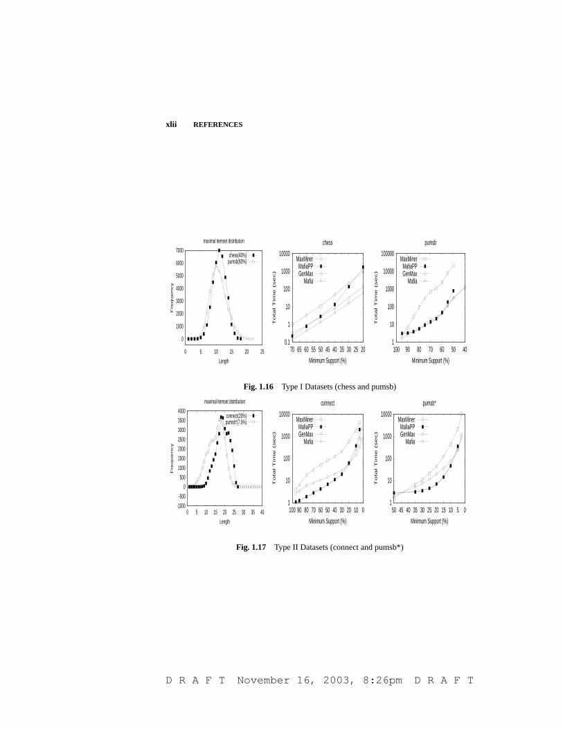
xlii REFERENCES
0
1000
2000
3000
4000
5000
6000
7000
0 5 10 15 20 25
Frequency
Length
maximal itemset distribution
chess(40%)pumsb(60%)
0.1
1
10
100
1000
10000
2025303540455055606570
Tota
l T
ime (
sec)
Minimum Support (%)
chess
MaxMinerMafiaPPGenMax
Mafia
1
10
100
1000
10000
100000
405060708090100
Tota
l T
ime (
sec)
Minimum Support (%)
pumsb
MaxMinerMafiaPPGenMax
Mafia
Fig. 1.16 Type I Datasets (chess and pumsb)
-1000
-500
0
500
1000
1500
2000
2500
3000
3500
4000
0 5 10 15 20 25 30 35 40
Frequency
Length
maximal itemset distribution
connect(20%)pumsb*(7.5%)
1
10
100
1000
10000
0102030405060708090100
Tota
l T
ime (
sec)
Minimum Support (%)
connect
MaxMinerMafiaPPGenMax
Mafia
1
10
100
1000
10000
05101520253035404550
Tota
l T
ime (
sec)
Minimum Support (%)
pumsb*
MaxMinerMafiaPPGenMax
Mafia
Fig. 1.17 Type II Datasets (connect and pumsb*)
D R A F T November 16, 2003, 8:26pm D R A F T
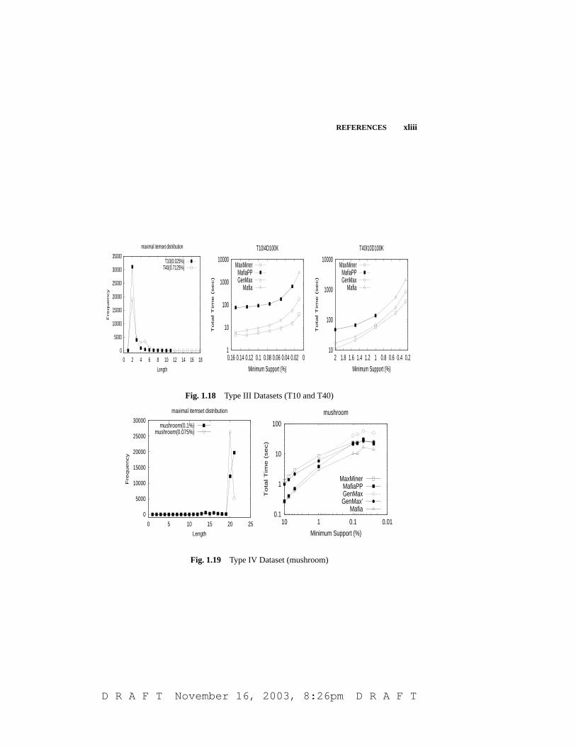
REFERENCES xliii
0
5000
10000
15000
20000
25000
30000
35000
0 2 4 6 8 10 12 14 16 18
Frequency
Length
maximal itemset distribution
T10(0.025%)T40(0.7125%)
1
10
100
1000
10000
00.020.040.060.080.10.120.140.16
Tota
l T
ime (
sec)
Minimum Support (%)
T10I4D100K
MaxMinerMafiaPPGenMax
Mafia
10
100
1000
10000
0.20.40.60.811.21.41.61.82
Tota
l T
ime (
sec)
Minimum Support (%)
T40I10D100K
MaxMinerMafiaPPGenMax
Mafia
Fig. 1.18 Type III Datasets (T10 and T40)
0
5000
10000
15000
20000
25000
30000
0 5 10 15 20 25
Fre
quency
Length
maximal itemset distribution
mushroom(0.1%)mushroom(0.075%)
0.1
1
10
100
0.010.1110
Tota
l T
ime (
sec)
Minimum Support (%)
mushroom
MaxMinerMafiaPPGenMaxGenMax’
Mafia
Fig. 1.19 Type IV Dataset (mushroom)
D R A F T November 16, 2003, 8:26pm D R A F T


![Research Article - Hindawi Publishing Corporation · 2019. 7. 30. · proposed such as maximal frequent patterns [6], top-k cooccurrence items with sequential pattern [7], weighted-based](https://static.fdocuments.net/doc/165x107/60df792032d81f7da10c673d/research-article-hindawi-publishing-corporation-2019-7-30-proposed-such-as.jpg)


