1 Linear in Parameters Models IV versus Control...
45
Imbens/Wooldridge, IRP Lecture Notes 14, August ’08 IRP Lectures Madison, WI, August 2008 Lecture 14, Tuesday, August 6, 9:30-10:45 Control Function and Related Methods These notes review the control function approach to handling endogeneity in models linear in parameters, and draws comparisons with standard methods such as 2SLS and maximum likelihood methods. Certain nonlinear models with endogenous explanatory variables are most easily estimated using the CF method, and the recent focus on average marginal effects suggests some simple, flexible strategies. Recent advances in semiparametric and nonparametric control function method are covered, and an example for how one can apply CF methods to nonlinear panel data models is provided. 1. Linear-in-Parameters Models: IV versus Control Functions Most models that are linear in parameters are estimated using standard instrumental variables methods – either two stage least squares (2SLS) or generalized method of moments (GMM). An alternative, the control function (CF) approach, relies on the same kinds of identification conditions. In the standard case where a endogenous explanatory variables appear linearly, the CF approach leads to the usual 2SLS estimator. But there are differences for models nonlinear in endogenous variables even if they are linear in parameters. And, for models nonlinear in parameters, the CF approach offers some distinct advantages. To illustrate the CF approach, let y 1 denote the response variable, y 2 the endogenous explanatory variable (a scalar for simplicity), and z the 1 L vector of exogenous variables (which includes unity as its first element). Consider the model y 1 z 1 1 1 y 2 u 1 , (1.1) 1
Transcript of 1 Linear in Parameters Models IV versus Control...
Imbens/Wooldridge, IRP Lecture Notes 14, August ’08
IRP Lectures Madison,WI, August 2008Lecture 14, Tuesday, August 6, 9:30-10:45
Control Function and Related Methods
These notes review the control function approach to handling endogeneity in models linear
in parameters, and draws comparisons with standard methods such as 2SLS and maximum
likelihood methods. Certain nonlinear models with endogenous explanatory variables are most
easily estimated using the CF method, and the recent focus on average marginal effects
suggests some simple, flexible strategies. Recent advances in semiparametric and
nonparametric control function method are covered, and an example for how one can apply CF
methods to nonlinear panel data models is provided.
1. Linear-in-Parameters Models: IV versus ControlFunctions
Most models that are linear in parameters are estimated using standard instrumental
variables methods – either two stage least squares (2SLS) or generalized method of moments
(GMM). An alternative, the control function (CF) approach, relies on the same kinds of
identification conditions. In the standard case where a endogenous explanatory variables
appear linearly, the CF approach leads to the usual 2SLS estimator. But there are differences
for models nonlinear in endogenous variables even if they are linear in parameters. And, for
models nonlinear in parameters, the CF approach offers some distinct advantages.
To illustrate the CF approach, let y1 denote the response variable, y2 the endogenous
explanatory variable (a scalar for simplicity), and z the 1 L vector of exogenous variables
(which includes unity as its first element). Consider the model
y1 z11 1y2 u1, (1.1)
1
Imbens/Wooldridge, IRP Lecture Notes 14, August ’08
where z1 is a 1 L1 strict subvector of z that also includes a constant. The sense in which z is
exogenous is given by the L orthogonality (zero covariance) conditions
Ez′u1 0. (1.2)
Of course, this is the same exogeneity condition that we use for consistency of the 2SLS
estimator, and we can consistently estimate 1 and 1 by 2SLS under (1.2) and the rank
condition, which reduces to rank Ez′x1 K1, where x1 z1,y2 is a 1 K1 vector. (We
also need to assume Ez′z is nonsingular, but this assumption is rarely a concern.)
Just as with 2SLS, the reduced form of y2 – that is, the linear projection of y2 onto the
exogenous variables – plays a critical role. Write the reduced form with an error term as
y2 z2 v2
Ez′v2 0 (1.3) (1.4)
where 2 is L 1. Endogeneity of y2 arises if and only if u1 is correlated with v2. Write the
linear projection of u1 on v2, in error form, as
u1 1v2 e1, (1.5)
where 1 Ev2u1/Ev22 is the population regression coefficient. By definition, Ev2e1 0,
and Ez′e1 0 because u1 and v2 are both uncorrelated with z.
Plugging (1.5) into equation (1.1) gives
y1 z11 1y2 1v2 e1, (1.6)
where we now view v2 as an explanatory variable in the equation. As just noted, e1, is
uncorrelated with v2 and z. Plus, y2 is a linear function of z and v2, and so e1 is also
uncorrelated with y2.
Because e1 is uncorrelated with z1, y2, and v2, (1.6) suggests a simple procedure for
2
Imbens/Wooldridge, IRP Lecture Notes 14, August ’08
consistently estimating 1 and 1 (as well as 1): run the OLS regression of y1 on z1,y2, and v2
using a random sample. (Remember, OLS consistently estimates the parameters in any
equation where the error term is uncorrelated with the right hand side variables.) The only
problem with this suggestion is that we do not observe v2; it is the error in the reduced form
equation for y2. Nevertheless, we can write v2 y2 − z2 and, because we collect data on y2
and z, we can consistently estimate 2 by OLS. Therefore, we can replace v2 with v2, the OLS
residuals from the first-stage regression of y2 on z. Simple substitution gives
y1 z11 1y2 1v2 error, (1.7)
where, for each i, errori ei1 1zi2 − 2, which depends on the sampling error in 2
unless 1 0. Standard results on two-step estimation imply the OLS estimators from (1.7)
will be consistent for 1,1, and 1.
The OLS estimates from (1.7) are control function estimates. The inclusion of the residuals
v2 “controls” for the endogeneity of y2 in the original equation (although it does so with
sampling error because 2 ≠ 2).
It is a simple exercise in the algebra of least squares to show that the OLS estimates of 1
and 1 from (1.7) are identical to the 2SLS estimates starting from (1.1) and using z as the
vector of instruments. [Standard errors from (1.7) must adjust for the generated regressor.]
It is trivial to use (1.7) to test H0 : 1 0, as the usual t statistic is asymptotically valid
under homoskedasticity Varu1|z,y2 12 under H0; or use the heteroskedasticity-robust
version (which does not account for the first-stage estimation of 2).
An estimator that can be different from the CF and 2SLS estimators is the limited
information (quasi-) maximum likelihood (LIML) estimator. The LIML estimator is obtained
from equations (1.1) and (1.3) under the assumption that u1,v2 is independent of z with a
3
Imbens/Wooldridge, IRP Lecture Notes 14, August ’08
mean-zero bivariate normal distribution. In fact, we can work off of (1.3) and (1.6) and use the
relationship fy1,y2|z fy1|y2,zfy2|z. If 12 Vare1 and 2
2 Varv2, the
quasi-log-likelihood for observation i is
− log12/2 − yi1 − zi11 − 1yi2 − 1yi2 − zi22/21
2
− log22/2 − yi2 − zi22/22
2, (1.8)
and all parameters are estimated simultaneously. When (1.1) is overidentified, LIML is
generally different from CF (2SLS). And, as the weak instruments notes document, LIML
typically has better statistical properties than 2SLS in situations with overidentification. The
CF approach can be seen to be a two-step version of LIML, where 2 is obtained in a first step
and then 1,1, and 1 are estimated in a second step. (The variance parameters can be
estimated in the two-step procedure, too.) Fortunately, while LIML is derived under joint
normality, it is just as robust as the CF estimator: independence between the errors and z and
normality are not needed.
[Incidentally, full information maximum likelihood (FIML) arises in systems with true
simultaneity when interest lies in estimating all structural equations. In these notes, we assume
that one equation is of particular interest. This could be because it is the main equation in a
truly simultaneous system or because the endogeneity we are worried about is due to omitted
variables.]
Now extend the model to include a quadratic:
y1 z11 1y2 1y22 u1
Eu1|z 0. (1.9) (1.10)
For simplicity, assume that we have a scalar, z2, that is not also in z1. Then, under (1.10) –
which is stronger than (1.2), and is essentially needed to identify nonlinear models – we can
4
Imbens/Wooldridge, IRP Lecture Notes 14, August ’08
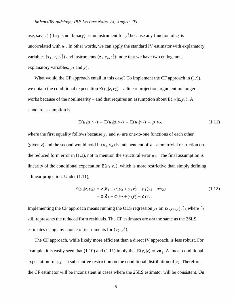
use, say, z22 (if z2 is not binary) as an instrument for y2
2 because any function of z2 is
uncorrelated with u1. In other words, we can apply the standard IV estimator with explanatory
variables z1,y2,y22 and instruments z1, z2, z2
2; note that we have two endogenous
explanatory variables, y2 and y22.
What would the CF approach entail in this case? To implement the CF approach in (1.9),
we obtain the conditional expectation Ey1|z,y2 – a linear projection argument no longer
works because of the nonlinearity – and that requires an assumption about Eu1|z,y2. A
standard assumption is
Eu1|z,y2 Eu1|z,v2 Eu1|v2 1v2, (1.11)
where the first equality follows because y2 and v2 are one-to-one functions of each other
(given z) and the second would hold if u1,v2 is independent of z – a nontrivial restriction on
the reduced form error in (1.3), not to mention the structural error u1.. The final assumption is
linearity of the conditional expectation Eu1|v2, which is more restrictive than simply defining
a linear projection. Under (1.11),
Ey1|z,y2 z11 1y2 1y22 1y2 − z2
z11 1y2 1y22 1v2.
(1.12)
Implementing the CF approach means running the OLS regression y1 on z1,y2,y22, v2,where v2
still represents the reduced form residuals. The CF estimates are not the same as the 2SLS
estimates using any choice of instruments for y2,y22.
The CF approach, while likely more efficient than a direct IV approach, is less robust. For
example, it is easily seen that (1.10) and (1.11) imply that Ey2|z z2. A linear conditional
expectation for y2 is a substantive restriction on the conditional distribution of y2. Therefore,
the CF estimator will be inconsistent in cases where the 2SLS estimator will be consistent. On
5
Imbens/Wooldridge, IRP Lecture Notes 14, August ’08
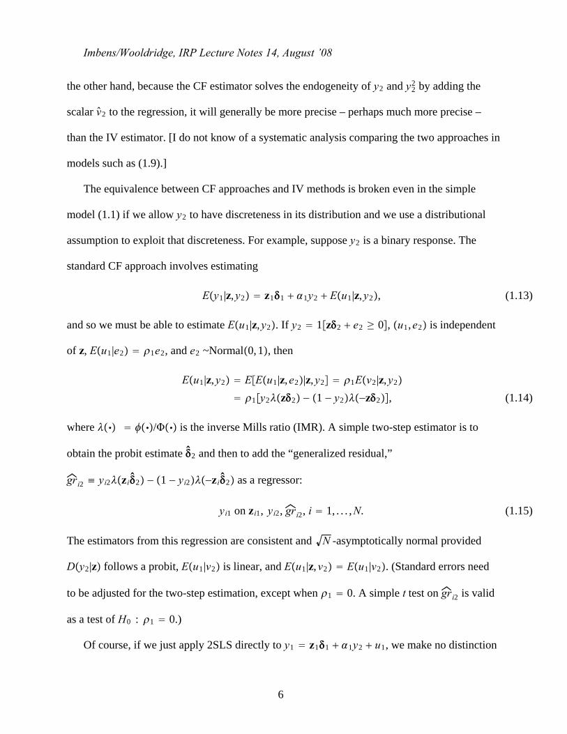
the other hand, because the CF estimator solves the endogeneity of y2 and y22 by adding the
scalar v2 to the regression, it will generally be more precise – perhaps much more precise –
than the IV estimator. [I do not know of a systematic analysis comparing the two approaches in
models such as (1.9).]
The equivalence between CF approaches and IV methods is broken even in the simple
model (1.1) if we allow y2 to have discreteness in its distribution and we use a distributional
assumption to exploit that discreteness. For example, suppose y2 is a binary response. The
standard CF approach involves estimating
Ey1|z,y2 z11 1y2 Eu1|z,y2, (1.13)
and so we must be able to estimate Eu1|z,y2. If y2 1z2 e2 ≥ 0, u1,e2 is independent
of z, Eu1|e2 1e2, and e2 ~Normal0,1, then
Eu1|z,y2 EEu1|z,e2|z,y2 1Ev2|z,y2
1y2z2 − 1 − y2−z2, (1.14)
where / is the inverse Mills ratio (IMR). A simple two-step estimator is to
obtain the probit estimate 2 and then to add the “generalized residual,”
gri2 ≡ yi2zi2 − 1 − yi2−zi2 as a regressor:
yi1 on zi1, yi2, gri2, i 1, . . . ,N. (1.15)
The estimators from this regression are consistent and N -asymptotically normal provided
Dy2|z follows a probit, Eu1|v2 is linear, and Eu1|z,v2 Eu1|v2. (Standard errors need
to be adjusted for the two-step estimation, except when 1 0. A simple t test on gri2 is valid
as a test of H0 : 1 0.)
Of course, if we just apply 2SLS directly to y1 z11 1y2 u1, we make no distinction
6
Imbens/Wooldridge, IRP Lecture Notes 14, August ’08
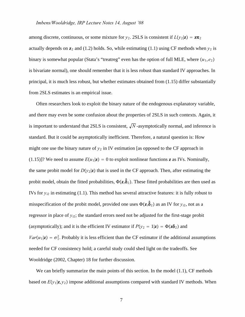
among discrete, continuous, or some mixture for y2. 2SLS is consistent if Ly2|z z2
actually depends on z2 and (1.2) holds. So, while estimating (1.1) using CF methods when y2 is
binary is somewhat popular (Stata’s “treatreg” even has the option of full MLE, where u1,e2
is bivariate normal), one should remember that it is less robust than standard IV approaches. In
principal, it is much less robust, but whether estimates obtained from (1.15) differ substantially
from 2SLS estimates is an empirical issue.
Often researchers look to exploit the binary nature of the endogenous explanatory variable,
and there may even be some confusion about the properties of 2SLS in such contexts. Again, it
is important to understand that 2SLS is consistent, N -asymptotically normal, and inference is
standard. But it could be asymptotically inefficient. Therefore, a natural question is: How
might one use the binary nature of y2 in IV estimation [as opposed to the CF approach in
(1.15)]? We need to assume Eu1|z 0 to exploit nonlinear functions z as IVs. Nominally,
the same probit model for Dy2|z that is used in the CF approach. Then, after estimating the
probit model, obtain the fitted probabilities, zi2. These fitted probabilities are then used as
IVs for yi2 in estimating (1.1). This method has several attractive features: it is fully robust to
misspecification of the probit model, provided one uses zi2 as an IV for yi2, not as a
regressor in place of yi2; the standard errors need not be adjusted for the first-stage probit
(asymptotically); and it is the efficient IV estimator if Py2 1|z z2 and
Varu1|z 12. Probably it is less efficient than the CF estimator if the additional assumptions
needed for CF consistency hold; a careful study could shed light on the tradeoffs. See
Wooldridge (2002, Chapter) 18 for further discussion.
We can briefly summarize the main points of this section. In the model (1.1), CF methods
based on Ey1|z,y2 impose additional assumptions compared with standard IV methods. When
7

Imbens/Wooldridge, IRP Lecture Notes 14, August ’08
y2 has special features (such as being binary, or even a corner solution), models for Ey2|z can
be used to generate instruments (not regressors) for y2. The resulting IV estimates are robust to
misspecification of the model for Ey2|z and the first-step estimation can be ignored
asymptotically.
8
Imbens/Wooldridge, IRP Lecture Notes 14, August ’08
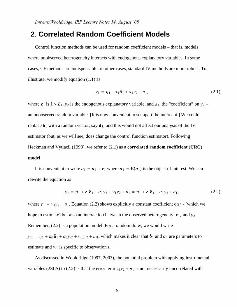
2. Correlated Random Coefficient ModelsControl function methods can be used for random coefficient models – that is, models
where unobserved heterogeneity interacts with endogenous explanatory variables. In some
cases, CF methods are indispensable; in other cases, standard IV methods are more robust. To
illustrate, we modify equation (1.1) as
y1 1 z11 a1y2 u1, (2.1)
where z1 is 1 L1, y2 is the endogenous explanatory variable, and a1, the “coefficient” on y2 –
an unobserved random variable. [It is now convenient to set apart the intercept.] We could
replace 1 with a random vector, say d1, and this would not affect our analysis of the IV
estimator (but, as we will see, does change the control function estimator). Following
Heckman and Vytlacil (1998), we refer to (2.1) as a correlated random coefficient (CRC)
model.
It is convenient to write a1 1 v1 where 1 Ea1 is the object of interest. We can
rewrite the equation as
y1 1 z11 1y2 v1y2 u1 ≡ 1 z11 1y2 e1, (2.2)
where e1 v1y2 u1. Equation (2.2) shows explicitly a constant coefficient on y2 (which we
hope to estimate) but also an interaction between the observed heterogeneity, v1, and y2.
Remember, (2.2) is a population model. For a random draw, we would write
yi1 1 zi11 1yi2 vi1yi2 ui1, which makes it clear that 1 and 1 are parameters to
estimate and vi1 is specific to observation i.
As discussed in Wooldridge (1997, 2003), the potential problem with applying instrumental
variables (2SLS) to (2.2) is that the error term v1y2 u1 is not necessarily uncorrelated with
9
Imbens/Wooldridge, IRP Lecture Notes 14, August ’08
the instruments z, even if we make the assumptions
Eu1|z Ev1|z 0, (2.3)
which we maintain from here on. Generally, the term v1y2 can cause problems for IV
estimation, but it is important to be clear about the nature of the problem. If we are allowing y2
to be correlated with u1 then we also want to allow y2 and v1 to be correlated. In other words,
Ev1y2 Covv1,y2 ≡ 1 ≠ 0. But a nonzero unconditional covariance is not a problem
with applying IV to (2.2): it simply implies that the composite error term, e1, has
(unconditional) mean 1 rather than a zero. As we know, a nonzero mean for e1 means that the
orginal intercept, 1, would be inconsistenly estimated, but this is rarely a concern.
Therefore, we can allow Covv1,y2, the unconditional covariance, to be unrestricted. But
the usual IV estimator is generally inconsistent if Ev1y2|z depends on z. Note that, because
Ev1|z 0, Ev1y2|z Covv1,y2|z. Therefore, as shown in Wooldridge (2003), a
sufficient condition for the IV estimator applied to (2.2) to be consistent for 1 and 1 is
Covv1,y2|z Covv1,y2. (2.4)
The 2SLS intercept estimator is consistent for 1 1. Condition (2.4) means that the
conditional covariance between v1 and y2 is not a function of z, but the unconditional
covariance is unrestricted.
Because v1 is unobserved, we cannot generally verify (2.4). But it is easy to find situations
where it holds. For example, if we write
y2 m2z v2 (2.5)
and assume v1,v2 is independent of z (with zero mean), then (2.4) is easily seen to hold
because Covv1,y2|z Covv1,v2|z, and the latter cannot be a function of z under
10
Imbens/Wooldridge, IRP Lecture Notes 14, August ’08
independence. Of course, assuming v2 in (2.5) is independent of z is a strong assumption even
if we do not need to specify the mean function, m2z. It is much stronger than just writing
down a linear projection of y2 on z (which is no real assumption at all). As we will see in
various models in Part IV, the representation (2.5) with v2 independent of z is not suitable for
discrete y2, and generally (2.4) is not a good assumption when y2 has discrete characteristics.
Further, as discussed in Card (2001), (2.4) can be violated even if y2 is (roughly) continuous.
Wooldridge (2005) makes some headway in relaxing (2.44) by allowing for parametric
heteroskedasticity in u1 and v2.
A useful extension of (1.1) is to allow observed exogenous variables to interact with y2.
The most convenient formulation is
y1 1 z11 1y2 z1 − 1y21 v1y2 u1 (2.6)
where 1 ≡ Ez1 is the 1 L1 vector of population means of the exogenous variables and 1
is an L1 1 parameter vector. As we saw in Chapter 4, subtracting the mean from z1 before
forming the interaction with y2 ensures that 1 is the average partial effect.
Estimation of (2.6) is simple if we maintain (2.4) [along with (2.3) and the appropriate rank
condition]. Typically, we would replace the unknown 1 with the sample averages, z1, and
then estimate
yi1 1 zi11 1yi2 zi1 − z1yi21 errori (2.7)
by instrumental variables, ignoring the estimation error in the population mean. The only issue
is choice of instruments, which is complicated by the interaction term. One possibility is to use
interactions between zi1 and all elements of zi (including zi1). This results in many
overidentifying restrictions, even if we just have one instrument zi2 for yi2. Alternatively, we
11
Imbens/Wooldridge, IRP Lecture Notes 14, August ’08
could obtain fitted values from a first stage linear regression yi2 on zi, ŷ i2 zi2, and then use
IVs 1,zi, zi1 − z1ŷ i2, which results in as many overidentifying restrictions as for the model
without the interaction. Importantly, the use of zi1 − z1ŷ i2 as IVs for zi1 − z1yi2 is
asymptotically the same as using instruments zi1 − 1 zi2, where Ly2|z z2 is the
linear projection. In other words, consistency of this IV procedure does not in any way restrict
the nature of the distribution of y2 given z. Plus, although we have generated instruments, the
assumptions sufficient for ignoring estimation of the instruments hold, and so inference is
standard (perhaps made robust to heteroskedasticity, as usual).
We can just identify the parameters in (2.6) by using a further restricted set of instruments,
1,zi1,ŷ i2, zi1 − z1ŷ i2. If so, it is important to use these as instruments and not as regressors.
If we add the assumption. The latter procedure essentially requires a new assumption:
Ey2|z z2 (2.8)
(where z includes a constant). Under (2.3), (2.4), and (2.8), it is easy to show
Ey1|z 1 1 z11 1z2 z1 − 1 z21, (2.9)
which is the basis for the Heckman and Vytlacil (1998) plug-in estimator. The usual IV
approach applied to (2.7) simply relaxes (2.8) and does not require adjustments to the standard
errors (because it uses generated instruments, not generated regressors).
We can also use a control function approach if we assume
Eu1|z,v2 1v2,Ev1|z,v2 1v2. (2.10)
Then
Ey1|z,y2 1 z11 1y2 1v2y2 1v2, (2.11)
and this equation is estimable once we estimate 2. Garen’s (1984) control function procedure
12
Imbens/Wooldridge, IRP Lecture Notes 14, August ’08
is to first regress y2 on z and obtain the reduced form residuals, v2, and then to run the OLS
regression y1 on 1,z1,y2, v2y2, v2. Under the maintained assumptions, Garen’s method
consistently estimates 1 and 1. Because the second step uses generated regressors, the
standard errors should be adjusted for the estimation of 2 in the first stage. Nevertheless, a
test that y2 is exogenous is easily obtained from the usual F test of H0 : 1 0,1 0 (or a
heteroskedasticity-robust version). Under the null, no adjustment is needed for the generated
standard errors.
Garen’s assumptions are more restrictive than those needed for the standard IV estimator to
be consistent. For one, it would be a fluke if (2.10) held without the conditional covariance
Covv1,y2|z being independent of z. Plus, like HV (1998), Garen relies on a linear model for
Ey2|z. Further, Garen adds the assumptions that Eu1|v2 and Ev1|v2 are linear functions,
something not needed by the IV approach.
Of course, one can make Garen’s approach less parametric by replacing the linear functions
in (2.10) with unknown functions. But independence of u1,v1,v2 and z – or something very
close to independence – is needed. And this assumption is not needed for the usual IV
estimator,
If the assumptions needed for Garen’s CF estimator to be consistent hold, it is likely more
efficient than the IV estimator, although a comparison of the correct asymptotic variances is
complicated. Again, there is a tradeoff between efficiency and robustness.
In the case of binary y2, we have what is often called the “switching regression” model.
Now, the right hand side of equation (2.11) represents Ey1|z,v2 where y2 1z2 v2 ≥ 0.
If we assume (2.10) and that v2|z is Normal0,1, then
Ey1|z,y2 1 z11 1y2 1h2y2,z2 1h2y2,z2y2, (2.12)
13
Imbens/Wooldridge, IRP Lecture Notes 14, August ’08
where
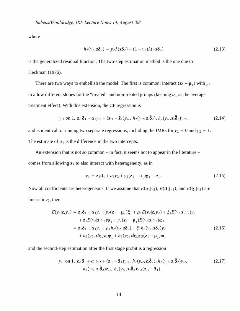
h2y2,z2 y2z2 − 1 − y2−z2 (2.13)
is the generalized residual function. The two-step estimation method is the one due to
Heckman (1976).
There are two ways to embellish the model. The first is common: interact z1 − 1 with y2
to allow different slopes for the “treated” and non-treated groups (keeping 1 as the average
treatment effect). With this extension, the CF regression is
yi1 on 1, zi11 1yi2 zi1 − z1yi2, h2yi2,zi2, h2yi2,zi2yi2, (2.14)
and is identical to running two separate regressions, including the IMRs for y2 0 and y2 1.
The estimate of 1 is the difference in the two intercepts.
An extension that is not so common – in fact, it seems not to appear in the literature –
comes from allowing z1 to also interact with heterogeneity, as in
y1 z1d1 a1y2 y2z1 − 1g1 u1. (2.15)
Now all coefficients are heterogeneous. If we assume that Ea1|v2, Ed1|v2, and Eg1|v2 are
linear in v2, then
Ey1|z,y2 z11 1y2 y2z1 − 11 1Ev2|z,y2 1Ev2|z,y2y2
z1Ev2|z,y21 y2z1 − 1Ev2|z,y21
z11 1y2 1h2y2,z2 1h2y2,z2y2
h2y2,z2z11 h2y2,z2y2z1 − 11
(2.16)
and the second-step estimation after the first stage probit is a regression
yi1 on 1, zi11 1yi2 zi1 − z1yi2, h2yi2,zi2, h2yi2,zi2yi2,h2yi2,zi2zi1, h2yi2,zi2yi2zi1 − z1.
(2.17)
14
Imbens/Wooldridge, IRP Lecture Notes 14, August ’08
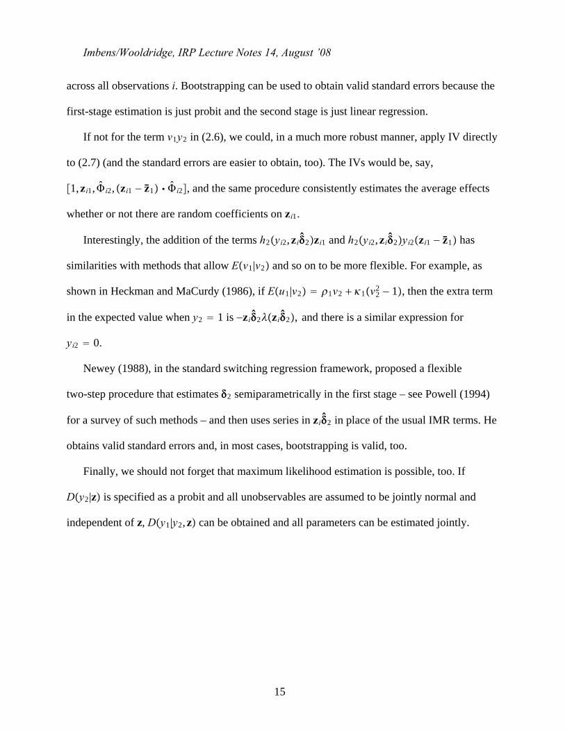
across all observations i. Bootstrapping can be used to obtain valid standard errors because the
first-stage estimation is just probit and the second stage is just linear regression.
If not for the term v1y2 in (2.6), we could, in a much more robust manner, apply IV directly
to (2.7) (and the standard errors are easier to obtain, too). The IVs would be, say,
1,zi1, i2, zi1 − z1 i2, and the same procedure consistently estimates the average effects
whether or not there are random coefficients on zi1.
Interestingly, the addition of the terms h2yi2,zi2zi1 and h2yi2,zi2yi2zi1 − z1 has
similarities with methods that allow Ev1|v2 and so on to be more flexible. For example, as
shown in Heckman and MaCurdy (1986), if Eu1|v2 1v2 1v22 − 1, then the extra term
in the expected value when y2 1 is −zi2zi2, and there is a similar expression for
yi2 0.
Newey (1988), in the standard switching regression framework, proposed a flexible
two-step procedure that estimates 2 semiparametrically in the first stage – see Powell (1994)
for a survey of such methods – and then uses series in zi2 in place of the usual IMR terms. He
obtains valid standard errors and, in most cases, bootstrapping is valid, too.
Finally, we should not forget that maximum likelihood estimation is possible, too. If
Dy2|z is specified as a probit and all unobservables are assumed to be jointly normal and
independent of z, Dy1|y2,z can be obtained and all parameters can be estimated jointly.
15
Imbens/Wooldridge, IRP Lecture Notes 14, August ’08
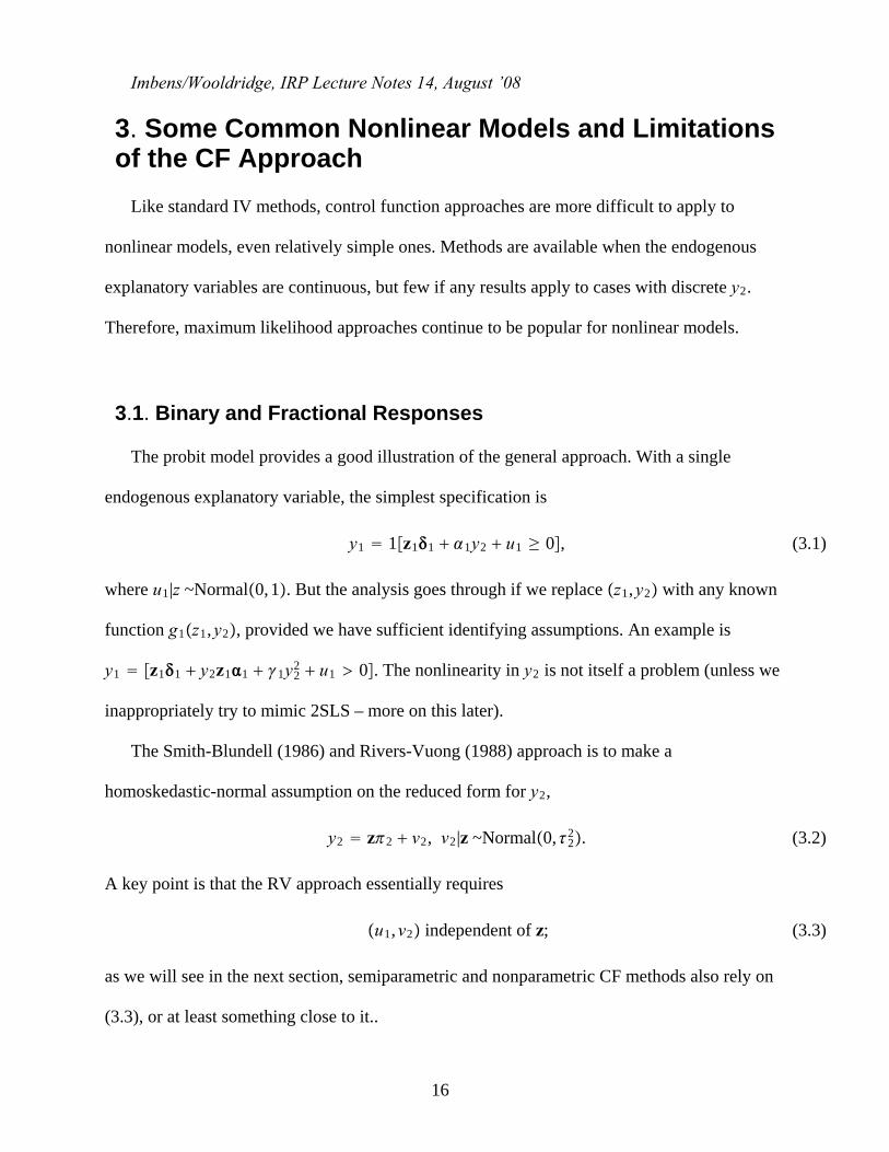
3. Some Common Nonlinear Models and Limitationsof the CF Approach
Like standard IV methods, control function approaches are more difficult to apply to
nonlinear models, even relatively simple ones. Methods are available when the endogenous
explanatory variables are continuous, but few if any results apply to cases with discrete y2.
Therefore, maximum likelihood approaches continue to be popular for nonlinear models.
3.1. Binary and Fractional Responses
The probit model provides a good illustration of the general approach. With a single
endogenous explanatory variable, the simplest specification is
y1 1z11 1y2 u1 ≥ 0, (3.1)
where u1|z ~Normal0,1. But the analysis goes through if we replace z1,y2 with any known
function g1z1,y2, provided we have sufficient identifying assumptions. An example is
y1 z11 y2z11 1y22 u1 0. The nonlinearity in y2 is not itself a problem (unless we
inappropriately try to mimic 2SLS – more on this later).
The Smith-Blundell (1986) and Rivers-Vuong (1988) approach is to make a
homoskedastic-normal assumption on the reduced form for y2,
y2 z2 v2, v2|z ~Normal0,22. (3.2)
A key point is that the RV approach essentially requires
u1,v2 independent of z; (3.3)
as we will see in the next section, semiparametric and nonparametric CF methods also rely on
(3.3), or at least something close to it..
16
Imbens/Wooldridge, IRP Lecture Notes 14, August ’08
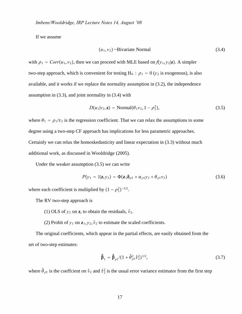
If we assume
u1,v2 ~Bivariate Normal (3.4)
with 1 Corru1,v2, then we can proceed with MLE based on fy1,y2|z. A simpler
two-step approach, which is convenient for testing H0 : 1 0 (y2 is exogenous), is also
available, and it works if we replace the normality assumption in (3.2), the independence
assumption in (3.3), and joint normality in (3.4) with
Du1|v2,z Normal1v2, 1 − 12, (3.5)
where 1 1/2 is the regression coefficient. That we can relax the assumptions to some
degree using a two-step CF approach has implications for less parametric approaches.
Certainly we can relax the homoskedasticity and linear expectation in (3.3) without much
additional work, as discussed in Wooldridge (2005).
Under the weaker assumption (3.5) we can write
Py1 1|z,y2 z11 1y2 1v2 (3.6)
where each coefficient is multiplied by 1 − 12−1/2.
The RV two-step approach is
(1) OLS of y2 on z, to obtain the residuals, v2.
(2) Probit of y1 on z1,y2, v2 to estimate the scaled coefficients.
The original coefficients, which appear in the partial effects, are easily obtained from the
set of two-step estimates:
1 1/1 12 2
21/2, (3.7)
where 1 is the coeffcient on v2 and 22 is the usual error variance estimator from the first step
17
Imbens/Wooldridge, IRP Lecture Notes 14, August ’08
OLS, and 1 includes 1 and 1. Standard errors can be obtained from the delta method of
bootstrapping. Of course, they are computed directly from MLE. Partial effects are based on
x11 where x1 z1,y2. It should be clear that nothing changes for estimation if
x1 g1z1,y2; of course, we would change how partial effects are computed to account for
the specific function g1, .
Testing the null hypothesis that y2 is exogenous is simple using the two-step control
function approache. Asymptotically, a simple t test on v2 is valid to test H0 : 1 0.
Under (3.3), we can also apply maximum likelihood by combining (3.2) and (3.6),
recognizing that v2 y2 − z2 and estimating all parameters jointly. For details, see
Wooldridge (2002, Section 15.7.2).
A different way to obtain partial effects is to use the average structural function approach,
which leads to estimation of Ev2x11 1v2. Whether or not v2 is normally distributed,
a consistent, N -asymptotically normal estimator of the average structural function (evaluated
at a given vector x1) is
ASFz1,y2 N−1∑i1
N
x11 1vi2; (3.8)
that is, we average out the reduced form residuals, vi2. This formulation is also useful for more
complicated models.
Given that the probit structural model is essentially arbitrary, one might be so bold as to
specify models for Py1 1|z1,y2,v2 directly. For example, we can add polynomials in v2 or
even interact v2 with elements of x1 side a probit or logit function. We return to such
possibilities in the next section.
18
Imbens/Wooldridge, IRP Lecture Notes 14, August ’08
The two-step CF approach easily extends to fractional responses. Now, we start with an
omitted variables formulation in the conditional mean:
Ey1|z,y2,q1 Ey1|z1,y2,q1 x11 q1, (3.9)
where x1 is a function of z1,y2 and q1 contains unobservables. As usual, we need some
exclusion restrictions, embodied by omitting z2 from x1. The specification in equation (3.9)
allows for responses at the corners, zero and one, and y1 may take on any values in between.
Under the assumption that
Dq1|v2,z ~ Normal1v2,12 (3.10)
Given (3.9) and (3.10), it can be shown, using the mixing property of the normal distribution,
that
Ey1|z,y2,v2 x11 1v2, (3.11)
where the index “” denotes coefficients multiplied by 1 12−1/2. Because the Bernoulli log
likelihood is in the linear exponential family, maximizing it consistently estimates the
parameters of a correctly specified mean; naturally, the same is true for two-step estimation.
That is, the same two-step method can be used in the binary and fractional cases. Of course,
the variance associated with the Bernoulli distribution is generally incorrect. In addition to
correcting for the first-stage estimates, a robust sandwich estimator should be computed to
account for the fact that Dy1|z,y2 is not Bernoulli. The best way to compute partial effects is
to use (3.8), with the slight notational change that the implicit scaling in the coefficients is
different. By using (3.8), we can directly use the scaled coefficients estimated in the second
stage – a feature common across CF methods for nonlinear models. The bootstrap that
reestimates the first and second stages for each iteration is an easy way to obtain standard
19
Imbens/Wooldridge, IRP Lecture Notes 14, August ’08
errors. Of course, having estimates of the parameters up to a common scale allows us to
determine signs of the partial effects in (3.9) as well as relative partial effects on the
continuous explanatory variables.
Wooldridge (2005) describes some simple ways to make the analysis starting from (3.9)
more flexible, including allowing Varq1|v2 to be heteroskedastic. We can also use strictly
monotonic transformations of y2 in the reduced form, say h2y2, regardless of how y2 appears
in the structural model: the key is that y2 can be written as a function of z,v2. The extension
to multivariate y2 is straightforward with sufficient instruments provide the elements of y2, or
strictly monotonic functions of them, have reduced forms with additive errors that are
effectively indendent of z. (This assumption rules out applications to y2 that are discrete
(binary, multinomial, or count)or have a discrete component (corner solution).
The control function approach has some decided advantages over another two-step
approach – one that appears to mimic the 2SLS estimation of the linear model. Rather than
conditioning on v2 along with z (and therefore y2) to obtain
Py1 1|z,v2 Py1 1|z,y2,v2, we can obtain Py1 1|z. To find the latter probability,
we plug in the reduced form for y2 to get y1 1z11 1z2 1v2 u1 0. Because
1v2 u1 is independent of z and u1,v2 has a bivariate normal distribution,
Py1 1|z z11 1z2/1 where
12 ≡ Var1v2 u1 1
222 1 21Covv2,u1. (A two-step procedure now proceeds by
using the same first-step OLS regression – in this case, to get the fitted values, ŷ i2 zi2 –
now followed by a probit of yi1 on zi1,ŷ i2. It is easily seen that this method estimates the
coefficients up to the common scale factor 1/1, which can be any positive value (unlike in the
CF case, where we know the scale factor is greater than unity).
20
Imbens/Wooldridge, IRP Lecture Notes 14, August ’08
One danger with plugging in fitted values for y2 is that one might be tempted to plug ŷ2
into nonlinear functions, say y22 or y2z1. This does not result in consistent estimation of the
scaled parameters or the partial effects. If we believe y2 has a linear RF with additive normal
error independent of z, the addition of v2 solves the endogeneity problem regardless of how y2
appears. Plugging in fitted values for y2 only works in the case where the model is linear in y2.
Plus, the CF approach makes it much easier to test the null that for endogeneity of y2 as well as
compute APEs.
In standard index models such as (3.9), or, if you prefer, (3.1), the use of control functions
to estimate the (scaled) parameters and the APEs produces no surprises. However, one must
take care when, say, we allow for random slopes in nonlinear models. For example, suppose
we propose a random coefficient model
Ey1|z,y2,c1 Ey1|z1,y2,c1 z11 a1y2 q1, (3.12)
where a1 is random with mean 1 and q1 again has mean of zero. If we want the partial effect
of y2, evaluated at the mean of heterogeneity, we have
1z11 1y2, (3.13)
where is the standard normal pdf, and this equation is obtained by differentiating (3.12)
with respect to y2 and then plugging in a1 1 and q1 0. Suppose we write a1 1 d1
and assume that d1,q1 is bivariate normal with mean zero. Then, for given z1,y2, the
average structural function can be shown to be
Ed1,q1z11 1y2 d1y2 q1 z11 1y2/1 q2 2dqy2 d2y221/2, (3.14)
where q2 Varq1, d2 Vard1, and dq Covd1,q1. The average partial effect with
respect to, say, y2, is the derivative of this function with respect to y2. While this partial effect
21
Imbens/Wooldridge, IRP Lecture Notes 14, August ’08
depends on 1, it is messier than (3.13) and need not even have the same sign as 1.
Wooldridge (2005) discusses related issues in the context of probit models with exogenous
variables and heteroskedasticity. In one example, he shows that, depending on whether
heteroskedasticity in the probit is due to heteroskedasticity in Varu1|x1, where u1 is the latent
error, or due to random slopes, the APEs are completely different in general. The same is true
here: the APE when the coefficient on y2 is random is generally very different from the APE
obtained if we maintain a1 1 but allow Varq1|v2 to be heteroskedastic. In the latter case,
the APE is a positive multiple of 1.
Incidentally, we can estimate the APE in (3.14) fairly generally. A parametric approach is
to assume joint normality of d1,q1,v2 (and independence with z). Then, with a normalization
restriction, it can be shown that
Ey1|z,v2 z11 1y2 1v2 1y2v2/1 1y2 1y221/2, (3.15)
which can be estimated by inserting v2 for v2 and using nonlinear least squares or Bernoulli
QMLE. (The latter is often called “heteroskedastic probit” when y1 is binary.) This procedure
can be viewed as an extension to Garen’s method for linear models with correlated random
coefficients.
Estimation, inference, and interpretation would be especially straightforward (the latter
possibly using the bootstrap) if we squint and pretend the term 1 1y2 1y221/2 is not
present. Then, estimation would simply be Bernoulli QMLE of yi1 on zi1, yi2, vi2, and yi2vi2,
which means that we just add the interaction to the usual Rivers-Vuong procedure. The APE
for y2 would be estimated by taking the derivative with respect to y2 and averaging out vi2, as
usual:
22
Imbens/Wooldridge, IRP Lecture Notes 14, August ’08
N−1∑i1
N
1 1vi2 z11 1y2 1vi2 1y2vi2, (3.16)
and evaluating this at chosen values for z1,y2 (or using further averaging across the sample
values). This simplification cannot be reconciled with (3.9), but it is in the spirit of adding
flexibility to a standard approach and treating functional forms as approximations. As a
practical matter, we can compare this with the APEs obtained from the standard Rivers-Vuong
approach, and a simple test of the null hypothesis that the coefficient on y2 is constant is
H0 : 1 0 (which should account for the first step estimation of 2). The null hypothesis
that y2 is exogenous is the joint test H0 : 1 0,1 0, and in this case no adjustment is
needed for the first-stage estimation. And why stop here? If we, add, say, y22 to the structural
model, we might add v22 to the estimating equation as well. It would be very difficult to relate
parameters estimated from the CF method to parameters in an underlying structural model;
indeed, it would be difficult to find a structural model given rise to this particular CF approach.
But if the object of interest are the average partial effects, the focus on flexible models for
Ey1|z1,y2,v2 can be liberating (or disturbing, depending on one’s point of view about
“structural” parameters).
Lewbel (2000) has made some progress in estimating parameters up to scale in the model
y1 1z11 1y2 u1 0, where y2 might be correlated with u1 and z1 is a 1 L1 vector
of exogenous variables. Lewbel’s (2000) general approach applies to this situation as well. Let
z be the vector of all exogenous variables uncorrelated with u1. Then Lewbel requires a
continuous element of z1 with nonzero coefficient – say the last element, zL1– that does not
appear in Du1|y2,z. (Clearly, y2 cannot play the role of the variable excluded from
Du1|y2,z if y2 is thought to be endogenous.) When might Lewbel’s exclusion restriction
23
Imbens/Wooldridge, IRP Lecture Notes 14, August ’08
hold? Sufficient is y2 g2z2 v2, where u1,v2 is independent of z and z2 does not contain
zL1 . But this means that we have imposed an exclusion restriction on the reduced form of y2,
something usually discouraged in parametric contexts. Randomization of zL1 does not make its
exclusion from the reduced form of y2 legitimate; in fact, one often hopes that an instrument
for y2 is effectively randomized, which means that zL1 does not appear in the structural
equation but does appear in the reduced form of y2 – the opposite of Lewbel’s assumption.
Lewbel’s assumption on the “special” regressor is suited to cases where a quantity that only
affects the response, y1, is randomized. A randomly generated project cost presented to
subjects in a willingness-to-pay study is one possibility. Even in such scenarios, one cannot
identify the effects of covariates on willingness to pay because coefficients are identified only
up to scale.
Returning to the probit response function in (3.9), we can understand the limits of the CF
approach for estimating nonlinear models with discrete EEVs. The Rivers-Vuong approach,
and its extension to fractional responses, cannot be expected to produce consistent estimates of
the parameters or APEs for discrete y2. The problem is that we cannot write
y2 z2 v2
Dv2|z Dv2 Normal0,22.
(3.17) (3.18)
In other words, unlike when we estimate a linear structural equation, the reduced form in the
RV approach is not just a linear projection – far from it. In the extreme we have completely
specified Dy2|z as homoskedastic normal, which is clearly violated if y2 is a binary variable,
a count variable, or a corner solution (commonly called a “censored” variable). Unfortunately,
even just assuming independence between v2 and z rules out discrete y2, an assumption that
plays an important role even in fully nonparametric approaches. The bottom line is that there
24
Imbens/Wooldridge, IRP Lecture Notes 14, August ’08
are no known two-step estimation methods that allow one to estimate a probit model or
fractional probit model with discrete y2, even if we make strong distributional assumptions.
Possibly because of the absense of valid two-step methods with discrete EEVs, some poor
strategies still linger. For example, suppose y1 and y2 are both binary, (3.1) holds, y2 follows
the index model
y2 1z2 v2 ≥ 0, (3.19)
and we maintain joint normality of u1,v2 – now both with unit variances – and, of course,
independence between the errors and z. Because Dy2|z follows a standard probit, it is
tempting to try to mimic 2SLS as follows: (i) Run probit of y2 on z and get the fitted
probabilities, 2 z2. (ii) Run probit of y1 on z1, 2; that is, just replace each yi2 with its
fitted probability, i2. This does not work, as it would require passing the expected value
passes through a nonlinear function. Some have called prodedures like this a “forbidden
regression.” We could find Ey1|z,y2 as a function of the structural and reduced form
parameters, insert the first-stage estimates of the RF parameters, and then use binary response
estimation in the second stage. But the estimator is not probit with the fitted probabilities
plugged in for y2. Currently, the only strategy we have is maximum likelihood estimation
based on fy1|y2,zfy2|z, which is not difficult. Wooldridge (2002, Section 15.7.3) contains
the likelihood function. [The dearth of options that allow some robustness to distributional
assumptions on y2 helps explain why some authors, notably Angrist (2001), have promoted the
idea of just using linear probability models estimated by 2SLS. This strategy seems to provide
good estimates of the average treatment effect in many applications. But it also seems true that
MLE based on joint normality might yield useful approximations to the APEs, too, even if the
distributional functions are not entirely correct. Such a view argues for fully robust inference
25
Imbens/Wooldridge, IRP Lecture Notes 14, August ’08
in the context of misspecified maximum likelihood, as in White (1982).]
An issue that comes up occasionally is whether “bivariate probit” software can be used to
estimate the probit model with a binary endogenous variable. In fact, the answer is yes, and the
endogenous variables can appear in any way in the model, particularly interacted with
exogenous variables. The key is that the likelihood function is constructed from
fy1|y2,x1f2y2|x2, and so its form does not change if x1 includes y2. (Of course, one should
have at least one exclusion restriction in the case x1 does depend on y2. ) MLE, of course, has
all of its desirable properties, and the parameter estimates needed to compute APEs are
provided directly.
If y1 is a fractional response satisfying (3.9), y2 follows (3.19), and q1,v2 are jointly
normal and independent of z, a two-step method based on Ey1|z,y2 is possible; the
expectation is not in closed form, and estimation cannot proceed by simply adding a control
function to a Bernoulli QMLE. But it should not be difficult to implement. Full MLE for a
fractional response is more difficult than for a binary response, particularly if y1 takes on
values at the endpoints with positive probability.
An essentially parallel discussion holds for ordered probit response models, where y1 takes
on the ordered values 0,1, . . . ,J. The RV procedure, and its extensions, applies immediately.
In computing partial effects on the response probabilities, we simply average out the reduced
for residuals, as in equation (3.8). The comments about the forbidden regression are
immediately applicable, too: one cannot simply insert, say, fitted probabilities for the binary
EEV y2 into an ordered probit model for y1 and hope for consistent estimates of anything of
interest.
Likewise, methods for Tobit models when y1 is a corner solution, such as labor supply or
26
Imbens/Wooldridge, IRP Lecture Notes 14, August ’08
charitable contributions, are analyzed in a similar fashion. If y2 is a continuous variable, CF
methods for consistent estimation can be obtained, at least under the assumptions used in the
RV setup. Smith and Blundell (1986) and Wooldridge (2002, Chapter 16) contain treatments.
The embellishments described above, such as letting Du1|v2 be a flexible normal distribution,
carry over immediately to Tobit case, as do the cautions in looking for simple two-step
methods when Dy2|z is discrete. Maximum likleihood estimation of all parameters jointly is
also quite feasible.
3.2. Multinomial and Ordered Responses
Allowing endogenous explanatory variables (EEVs) in multinomial response models is
notoriously difficult, even for continuous endogenous variables. There are two basic reasons.
First, multinomial probit (MNP), which mixes well well a reduced form normality assumption
for Dy2|z, is still computationally difficult for even a moderate number of choices.
Apparently, no one has undertaken a systematic treatment of MNP with EEVs, including how
to obtain partial effects.
The multinomial logit (MNL) model and its extensions, such as nested logit and random
coefficient versions, are much simpler computationally with lots of alternatives. Unfortunately,
the normal distribution does not mix well with the extreme value distribution, and so, if we
begin with a structural MNL model (or conditional logit), the estimating equations obtained
from a CF approach are difficult to obtain, and MLE is very difficult, too, even if we assume a
normal distribution in the reduced form(s).
Recently, some authors have suggested taking a practical approach to allowing continuous
EEVs in multinomial response. The suggestions for binary and fractional responses in the
27
Imbens/Wooldridge, IRP Lecture Notes 14, August ’08
previous subsection – namely, use probit, or even logit, with flexible functions of both the
observed variables and the reduced form residuals – is in this spirit.
Again it is convenient to model the source of endogeneity as an omitted variable. Let y1 be
the (unordered) multinomial response taking values 0,1, . . . ,J, let z be the vector of
endogenous variables, and let y2 be a vector of endogenous variables. If r1 represents omitted
factors that the researcher would like to control for, then the structural model consists of
specifications for the response probabilities
Py1 j|z1,y2, r1, j 0,1, . . . ,J. (3.20)
The average partial effects, as usual, are obtained by averaging out the unobserved
heterogeneity, r1. Assume that y2 follows the linear reduced form
y2 z2 v2. (3.21)
Typically, at least as a first attempt, we would assume a convenient joint distribution for
r1,v2, such as multivariate normal and independent of z. This approach has been applied
when the response probabilities, conditional on r1, have the conditional logit form. For
example, Villas-Boas and Winer (1999) apply this approach to modeling brand choice, where
prices are allowed to correlated with unobserved tastes that affect brand choice. In
implementing the CF approach, the problem in starting with a multinomial or conditional logit
model for (3.20) is computational. Nevertheless, estimation is possible, particular if one uses
simulation methods of estimation briefly mentioned in the previous subsection.
A much simpler control function approach is obtained if we skip the step of modeling
Py1 j|z1,y2, r1 and jump directly to convenient models for
Py1 j|zi1,y2,v2 Py1 j|z,y2. Petrin and Train (2006) are proponents of this solution.
28
Imbens/Wooldridge, IRP Lecture Notes 14, August ’08
The idea is that any parametric model for Py1 j|z1,y2, r1 is essentially arbitrary, so, if we
can recover quantities of interest directly from Py1 j|z1,y2,v2, why not specify these
probabilities directly? If we assume that Dr1|z,y2 Dr1|v2, and that Py1 j|z1,y2,v2
can be obtained from Py1 j|z1,y2, r1 by integrating the latter with respect to Dr1|v2 then
we can estimate the APEs directly from Py1 j|z1,y2,v2 by averaging out across the
reduced form residuals, as in previous cases.
Once we have selected a model for Py1 j|z1,y2,v2, which could be multinomial logit,
conditional logit, or nested logit, we can apply a simple two-step procedure. First, estimate the
reduced form for yi2 and obtain the residuals, vi2 yi2 − zi2. (Alternatively, we can use
strictly monotonic transformations of the elements of yi2.) Then, we estimate a multinomial
response model with explanatory variables zi1,yi2, and vi2. As always with control function
approaches, we need enough exclusion restrictions in zi1 to identify the parameters and APEs.
We can include nonlinear functions of zi1,yi2, vi2, including quadratics and interactions for
more flexibility.
Given estimates of the probabilities pjz1,y2,v2, we can estimate the average partial
effects on the structural probabilities by estimating the average structural function:
ASFz1,y2 N−1∑i1
N
pjz1,y2, vi2. (3.22)
Then, we can take derivatives or changes of ASFz1,y2 with respect to elements of z1,y2,
as usual. While the delta method can be used to obtain analytical standard errors, the bootstrap
is simpler and feasible if one uses, say, conditional logit.
In an application to choice of television service, Petrin and Train (2006) find the CF
29
Imbens/Wooldridge, IRP Lecture Notes 14, August ’08
approach gives remarkably similar parameter estimates to the approach proposed by Berry,
Pakes, and Levinsohn (1995), which we touch on in the cluster sample notes.
When the EEVs are discrete, the CF arguments above do not apply. One can often
implement maximum likelihood without too much difficulty. For example, Adams, Chiang,
and Jensen (2003) use MLE when the scalar y2 follows an ordered probit.
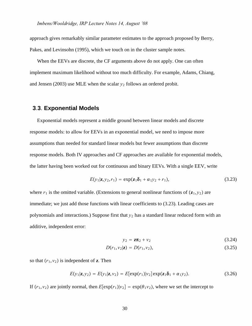
3.3. Exponential Models
Exponential models represent a middle ground between linear models and discrete
response models: to allow for EEVs in an exponential model, we need to impose more
assumptions than needed for standard linear models but fewer assumptions than discrete
response models. Both IV approaches and CF approaches are available for exponential models,
the latter having been worked out for continuous and binary EEVs. With a single EEV, write
Ey1|z,y2, r1 expz11 1y2 r1, (3.23)
where r1 is the omitted variable. (Extensions to general nonlinear functions of z1,y2 are
immediate; we just add those functions with linear coefficients to (3.23). Leading cases are
polynomials and interactions.) Suppose first that y2 has a standard linear reduced form with an
additive, independent error:
y2 z2 v2
Dr1,v2|z Dr1,v2, (3.24) (3.25)
so that r1,v2 is independent of z. Then
Ey1|z,y2 Ey1|z,v2 Eexpr1|v2expz11 1y2. (3.26)
If r1,v2 are jointly normal, then Eexpr1|v2 exp1v2, where we set the intercept to
30
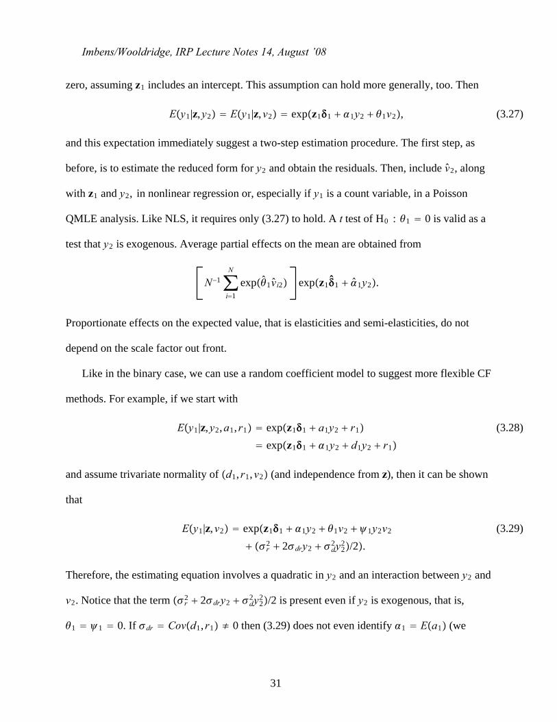
Imbens/Wooldridge, IRP Lecture Notes 14, August ’08
zero, assuming z1 includes an intercept. This assumption can hold more generally, too. Then
Ey1|z,y2 Ey1|z,v2 expz11 1y2 1v2, (3.27)
and this expectation immediately suggest a two-step estimation procedure. The first step, as
before, is to estimate the reduced form for y2 and obtain the residuals. Then, include v2, along
with z1 and y2, in nonlinear regression or, especially if y1 is a count variable, in a Poisson
QMLE analysis. Like NLS, it requires only (3.27) to hold. A t test of H0 : 1 0 is valid as a
test that y2 is exogenous. Average partial effects on the mean are obtained from
N−1∑i1
N
exp1vi2 expz11 1y2.
Proportionate effects on the expected value, that is elasticities and semi-elasticities, do not
depend on the scale factor out front.
Like in the binary case, we can use a random coefficient model to suggest more flexible CF
methods. For example, if we start with
Ey1|z,y2,a1, r1 expz11 a1y2 r1
expz11 1y2 d1y2 r1
(3.28)
and assume trivariate normality of d1, r1,v2 (and independence from z), then it can be shown
that
Ey1|z,v2 expz11 1y2 1v2 1y2v2
r2 2dry2 d2y22/2.
(3.29)
Therefore, the estimating equation involves a quadratic in y2 and an interaction between y2 and
v2. Notice that the term r2 2dry2 d2y22/2 is present even if y2 is exogenous, that is,
1 1 0. If dr Covd1, r1 ≠ 0 then (3.29) does not even identify 1 Ea1 (we
31
Imbens/Wooldridge, IRP Lecture Notes 14, August ’08
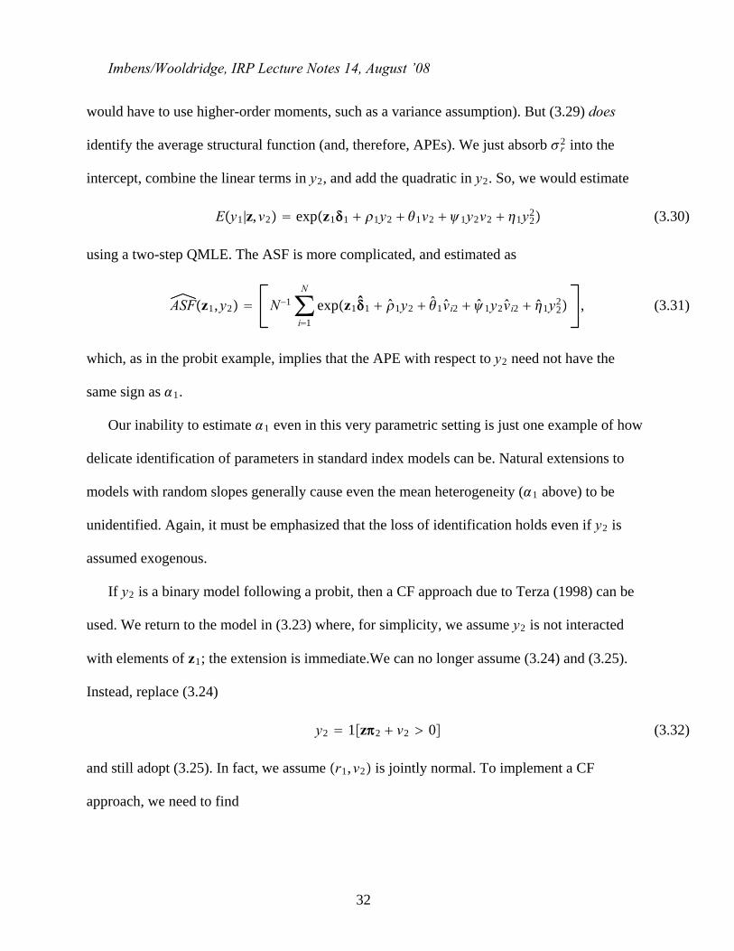
would have to use higher-order moments, such as a variance assumption). But (3.29) does
identify the average structural function (and, therefore, APEs). We just absorb r2 into the
intercept, combine the linear terms in y2, and add the quadratic in y2. So, we would estimate
Ey1|z,v2 expz11 1y2 1v2 1y2v2 1y22 (3.30)
using a two-step QMLE. The ASF is more complicated, and estimated as
ASFz1,y2 N−1∑i1
N
expz11 1y2 1vi2 1y2vi2 1y22 , (3.31)
which, as in the probit example, implies that the APE with respect to y2 need not have the
same sign as 1.
Our inability to estimate 1 even in this very parametric setting is just one example of how
delicate identification of parameters in standard index models can be. Natural extensions to
models with random slopes generally cause even the mean heterogeneity (1 above) to be
unidentified. Again, it must be emphasized that the loss of identification holds even if y2 is
assumed exogenous.
If y2 is a binary model following a probit, then a CF approach due to Terza (1998) can be
used. We return to the model in (3.23) where, for simplicity, we assume y2 is not interacted
with elements of z1; the extension is immediate.We can no longer assume (3.24) and (3.25).
Instead, replace (3.24)
y2 1z2 v2 0 (3.32)
and still adopt (3.25). In fact, we assume r1,v2 is jointly normal. To implement a CF
approach, we need to find
32
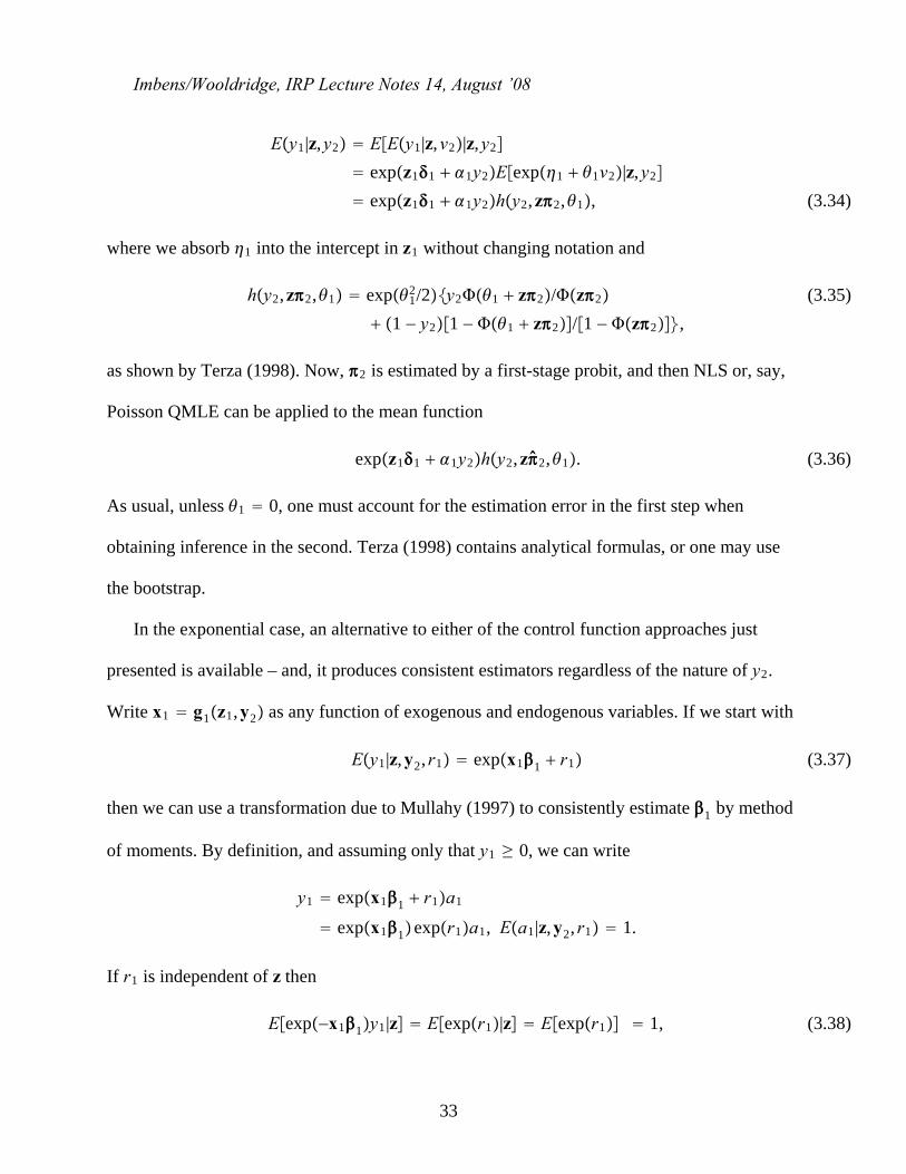
Imbens/Wooldridge, IRP Lecture Notes 14, August ’08
Ey1|z,y2 EEy1|z,v2|z,y2
expz11 1y2Eexp1 1v2|z,y2
expz11 1y2hy2,z2,1, (3.34)
where we absorb 1 into the intercept in z1 without changing notation and
hy2,z2,1 exp12/2y21 z2/z2
1 − y21 − 1 z2/1 − z2, (3.35)
as shown by Terza (1998). Now, 2 is estimated by a first-stage probit, and then NLS or, say,
Poisson QMLE can be applied to the mean function
expz11 1y2hy2,z2,1. (3.36)
As usual, unless 1 0, one must account for the estimation error in the first step when
obtaining inference in the second. Terza (1998) contains analytical formulas, or one may use
the bootstrap.
In the exponential case, an alternative to either of the control function approaches just
presented is available – and, it produces consistent estimators regardless of the nature of y2.
Write x1 g1z1,y2 as any function of exogenous and endogenous variables. If we start with
Ey1|z,y2, r1 expx11 r1 (3.37)
then we can use a transformation due to Mullahy (1997) to consistently estimate 1 by method
of moments. By definition, and assuming only that y1 ≥ 0, we can write
y1 expx11 r1a1
expx11expr1a1, Ea1|z,y2, r1 1.
If r1 is independent of z then
Eexp−x11y1|z Eexpr1|z Eexpr1 1, (3.38)
33
Imbens/Wooldridge, IRP Lecture Notes 14, August ’08
where the last equality is just a normalization that defines the intercept in 1. Therefore, we
have conditional moment conditions
Eexp−x11y1 − 1|z 0, (3.39)
which depends on the unknown parameters 1 and observable data. Any function of z can be
used as instruments in a nonlinear GMM procedure. An important issue in implementing the
procedure is choosing instruments. See Mullahy (1997) for further discussion.
4. Semiparametric and Nonparametric ApproachesBlundell and Powell (2004) show how to relax distributional assumptions on u1,v2 in the
model model y1 1x11 u1 0, where x1 can be any function of z1,y2. The key
assumption is that y2 can be written as y2 g2z v2, where u1,v2 is independent of z. The
independence of the additive error v2 and z pretty much rules out discreteness in y2, even
though g2 can be left unspecified. Under the independence assumption,
Py1 1|z,v2 Ey1|z,v2 Hx11,v2 (4.1)
for some (generally unknown) function H, . The average structural function is just
ASFz1,y2 Evi2Hx11,vi2. We can estimate H and 1 quite generally by first estimating
the function g2 and then obtaining residuals vi2 yi2 − ĝ2zi. Blundell and Powell (2004)
show how to estimate H and 1 (up to scale) and G, the distribution of u1. The ASF is
obtained from Gx11. We can also estimate the ASF by averaging out the reduced form
residuals,
34
Imbens/Wooldridge, IRP Lecture Notes 14, August ’08
ASFz1,y2 N−1∑i1
N
Ĥx11, vi2; (4.2)
derivatives and changes can be computed with respect to elements of z1,y2.
Blundell and Powell (2003) allow Py1 1|z,y2 to have the general form Hz1,y2,v2,
and then the second-step estimation is entirely nonparametric. They also allow ĝ2 to be fully
nonparametric. But parametric approximations in each stage might produce good estimates of
the APEs. For example, yi2 can be regressed on flexible functions of zi to obtain vi2. Then, one
can estimate probit or logit models in the second stage that include functions of z1, y2, and v2
in a flexible way – for example, with levels, quadratics, interactions, and maybe even
higher-order polynomials of each. Then, one simply averages out vi2, as in equation (4.2).
Valid standard errors and test statistics can be obtained by bootstrapping or by using the delta
method.
In certain cases, an even more parametric approach suggests itself. Suppose we have the
exponential regression
Ey1|z,y2, r1 expx11 r1, (4.3)
where r1 is the unobservable. If y2 g2z2 v2 and r1,v2 is independent of z, then
Ey1|z1,y2,v2 h2v2expx11, (4.4)
where now h2 is an unknown function. It can be approximated using series, say, and, of
course, first-stage residuals v2 replace v2.
Blundell and Powell (2003) consider a very general setup, which starts with
y1 g1z1,y2,u1, and then discuss estimation of the ASF, given by
ASF1z1,y2 g1z1,y2,u1dF1u1, (4.5)
35
Imbens/Wooldridge, IRP Lecture Notes 14, August ’08
where F1 is the distribution of u1. The key restrictions are that y2 can be written as
y2 g2z v2, (4.6)
where u1,v2 is independent of z. The additive, independent reduced form errors in (4.6)
effectively rule out applications to discrete y2. Conceptually, Blundell and Powell’s method is
straightforward, as it is a nonparametric extenstion of parametric approaches. First, estimate g2
nonparametrically (which, in fact, may be done via a flexible parametric model, or kernel
estimators). Obtain the residuals vi2 yi2 − ĝ2zi. Next, estimate
Ey1|z1,y2,v2 h1z1,y2,v2 using nonparametrics, where vi2 replaces v2. Identification of
h1 holds quite generally, provided we have sufficient exclusion restrictions (elements in z not
in z1. BP discuss some potential pitfalls. Once we have ĥ1, we can consistently estimate the
ASF. For given x1o z1
o,y2o, the ASF can always be written, using iterated expectations, as
Ev2Eg1x1o,u1|v2.
Under the assumption that u1,v2 is independent of z, Eg1x1o,u1|v2 h1x1
o,v2 – that is,
the regression function of y1 on x1,v2. Therefore, a consistent estimate of the ASF is
N−1∑i1
N
ĥ1x1, vi2. (4.7)
While semiparametric and parametric methods when y2 (or, more generally, a vector y2)
are continuous – actually, have a reduced form with an additive, independent error – they do
not currently help us with discrete EEVs.
With univariate y2, it possible to relax the additivity of v2 in the reduced form equation
under monotonicity assumptions. Like Blundell and Powell (2003), Imbens and Newey (2006)
consider the triangular system, but without additivity in the reduced form of y2. The structureal
36
Imbens/Wooldridge, IRP Lecture Notes 14, August ’08
equation is
y1 g1z1,y2,u1, (4.8)
where u1 is a vector heterogeneity (whose dimension may not even be known), and the
reduced form for y2 is
y2 g2z,e2, (4.9)
where g2z, is strictly monotonic. This assumption rules out discrete y2 but allows some
interaction between the unobserved heterogeneity in y2 and the exogenous variables. As one
special case, Imbens and Newey show that, if u1,e2 is assumed to be independent of z, then a
valid control function that can be used in a second stage is v2 ≡ Fy2|zy2,z, where Fy2|z is the
conditional distribution of y2 given z. Imbens and Newey described identification of various
quantities of interest, including the quantile structural function. When u1 is a scalar and
monotonically increasing in u1, the QSF is
QSFx1 g1x1,Quantu1, (4.10)
where Quantu1 is the th of u1. We consider quantile methods in more detail in the quantile
methods notes.
5. Methods for Panel DataWe can combine methods for handling correlated random effects models with control
function methods to estimate certain nonlinear panel data models with unobserved
heterogeneity and EEVs. Here we provide as an illustration a parametric approach used by
Papke and Wooldridge (2008), which applies to binary and fractional responses. The
37
Imbens/Wooldridge, IRP Lecture Notes 14, August ’08
manipulations are routine but point to more flexible ways of estimating the average marginal
effects. It is important to remember that we currently have no way of estimating, say,
unobserved effects models for fractional response variables, either with or without endogenous
explanatory variables, without imposing some restrictions on the distribution of heterogeneity
given the exogenous variables. Even the approaches that treat the unobserved effects as
parameters – and use large T approximations – to not allow endogenous regressors. Plus, recall
from the nonlinear panel data notes that most results are for the case where the data are
assumed independent across time. Jackknife approaches further assume homogeneity across
time.
We write the model with time-constant unobserved heterogeneity, ci1, and time-varying
unobservables, vit1, as
Eyit1|yit2,zi,ci1,vit1 Eyit1|yit2,zit1,ci1,vit1 1yit2 zit11 ci1 vit1. (5.1)
Thus, there are two kinds of potential omitted variables. We allow the heterogeneity, ci1, to be
correlated with yit2 and zi, where zi zi1, . . . ,ziT is the vector of strictly exogenous variables
(conditional on ci1). The time-varying omitted variable is uncorrelated with zi – strict
exogeneity – but may be correlated with yit2. As an example, yit1 is a female labor force
participation indicator and yit2 is other sources of income. Or, yit1 is a test pass rate, and the
school leve, and yit2 is a measure of spending per student.
When we write zit zit1,zit2, we are assuming zit2 can be excluded from the “structural”
equation (4.1). This is the same as the requirement for fixed effects two stage least squares
estimation of a linear model.
To proceed, we first model the heterogeneity using a Chamberlain-Mundlak approach:
38
Imbens/Wooldridge, IRP Lecture Notes 14, August ’08
ci1 1 zi1 ai1,ai1|zi ~ Normal0,a12 . (5.2)
We could allow the elements of zi to appear with separate coefficients, too. Note that only
exogenous variables are included in zi. Plugging into (5.1) we have
Eyit1|yit2,zi,ai1,vit1 1yit2 zit11 1 zi1 ai1 vit1
≡ 1yit2 zit11 1 zi1 rit1. (5.3)
Next, we assume a linear reduced form for yit2:
yit2 2 zit2 zi2 vit2, t 1, . . . ,T, (5.4)
where, if necessary, we can allow the coefficients in (5.4) to depend on t. The addition of the
time average of the strictly exogenous variables in (5.4) follows from the Mundlak (1978)
device. The nature of endogeneity of yit2 is through correlation between rit1 ai1 vit1 and
the reduced form error, vit2. Thus, yit2 is allowed to be correlated with unobserved
heterogeneity and the time-varying omitted factor. We also assume that rit1 given vit2 is
conditionally normal, which we write as
rit1 1vit2 eit1, (5.5)
eit1|zi,vit2 ~ Normal0,e12 , t 1, . . . ,T. (5.6)
Because eit1 is independent of zi,vit2, it is also independent of yit2. Using a standard mixing
property of the normal distribution,
Eyit1|zi,yit2,vit2 e1yit2 zit1e1 e1 zie1 e1vit2 (5.7)
where the “e” subscript denotes division by 1 e12 1/2. This equation is the basis for CF
estimation.
The assumptions used to obtain (5.7) would not hold for yit2 having discreteness or
39
Imbens/Wooldridge, IRP Lecture Notes 14, August ’08
substantively limited range in its distribution. It is straightfoward to include powers of vit2 in
(5.7) to allow greater flexibility. Following Wooldridge (2005) for the cross-sectional case, we
could even model rit1 given vit2 as a heteroskedastic normal.
In deciding on estimators of the parameters in (5.7), we must note that the explanatory
variables, while contemporaneous exogenous by construction, are not usually strictly
exogenous. In particular, we allow yis2 to be correlated with vit1 for t ≠ s. Therefore,
generalized estimation equations, that assume strict exogeneity – see the notes on nonlinear
panel data models – will not be consistent in general. We could apply method of moments
procedures. A simple approach is to use use pooled nonlinear least squares or pooled
quasi-MLE, using the Bernoulli log likelihood. (The latter fall under the rubric of generalized
linear models.) Of course, we want to allow arbitrary serial dependence and
Varyit1|zi,yit2,vit2 in obtaining inference, which means using a robust sandwich estimator.
The two step procedure is (i) Estimate the reduced form for yit2 (pooled across t, or maybe
for each t separately; at a minimum, different time period intercepts should be allowed).
Obtain the residuals, vit2 for all i, t pairs. The estimate of 2 is the fixed effects estimate. (ii)
Use the pooled probit QMLE of yit1 on yit2,zit1, zi, vit2 to estimate e1,e1,e1,e1 and e1.
Because of the two-step procedure, the standard errors in the second stage should be
adjusted for the first stage estimation. Alternatively, bootstrapping can be used by resampling
the cross-sectional units. Conveniently, if e1 0, the first stage estimation can be ignored, at
least using first-order asymptotics. Consequently, a test for endogeneity of yit2 is easily
obtained as an asymptotic t statistic on vit2; it should be make robust to arbitrary serial
correlation and misspecified variance. Adding first-stage residuals to test for endogeneity of an
explanatory variables dates back to Hausman (1978). In a cross-sectional contexts, Rivers and
40
Imbens/Wooldridge, IRP Lecture Notes 14, August ’08
Vuong (1988) suggested it for the probit model.
Estimates of average partial effects are based on the average structural function
Eci1,vit1 1yt2 zt11 ci1 vit1 (5.8)
with respect to the elements of yt2,zt1. It can be shown that
Ezi,vit2 e1yt2 zt1e1 e1 zie1 e1vit2; (5.9)
that is, we “integrate out” zi,vit2 and then take derivatives or changes with respect to the
elements of zt1yt2. Because we are not making a distributional assumption about zi,vit2, we
instead estimate the APEs by averaging out zi, vit2 across the sample, for a chosen t:
N−1∑i1
N
e1yt2 zt1e1 e1 zie1 e1vit2. (5.10)
APEs computed from (5.10) – typically with further averaging out across t and the values
of yt2 and zt1 – can be compared directly with linear model estimates, particular fixed effects
IV estimates.
We can use the approaches of Altonji and Matzkin (2005) and Blundell and Powell (2003)
to make the analysis less parametric. For example, we might replace (5.4) with
yit2 g2zit, zi vit2 (or use functions in addition to , zi, as in AM). Then, we could maintain
Dci1 vit1|zi,yit2 Dci1 vit1|zi,vit2.
In the first estimation step, vit2 is obtained from a nonparametric or semiparametric pooled
estimation. Then the function
Eyit1|yit2,zi,vit2 h1xit11, zi,vit2
can be estimated in a second stage, with the first-stage residuals, vit2, inserted. Generally,
41

Imbens/Wooldridge, IRP Lecture Notes 14, August ’08
identification holds because the vit2 varying over time separately from xit1 due to time-varying
exogenous instruments zit2. The inclusion of zi requires that we have at least one time-varying,
strictly exogenous instrument for yit2.
42
Imbens/Wooldridge, IRP Lecture Notes 14, August ’08
ReferencesAdams, J.D., E.P. Chiang, and J.L. Jensen (2003), “The Influence of Federal Laboratory
R&D on Industrial Research,” Review of Economics and Statistics 85, 1003-1020.
Altonji, J.G. and R.L. Matzkin (2005), “Cross Section and Panel Data Estimators for
Nonseparable Models with Endogenous Regressors,” Econometrica 73, 1053-1102.
Angrist, J.D. (1991), “Estimations of Limited Dependent Variable Models with Dummy
Endogenous Regressors: Simple Strategies for Empirical Practice,” Journal of Business and
Economic Statistics 19, 2-16.
Berry, S., J. Levinsohn, and A. Pakes (1995), “Automobile Prices in Market Equilibrium,”
Econometrica 63, 841-890.
Blundell, R. and J.L. Powell (2003), “Endogeneity in Nonparametric and Semiparametric
Regression Models,” in Advances in Economics and Econonometrics: Theory and
Applications, Eighth World Congress, Volume 2, M. Dewatripont, L.P. Hansen and S.J.
Turnovsky, eds. Cambridge: Cambridge University Press, 312-357.
Blundell, R. and J.L. Powell (2004), “Endogeneity in Semiparametric Binary Response
Models,” Review of Economic Studies 71, 655-679.
Card, D. (2001), “Estimating the Return to Schooling: Progress on Some Persistent
Econometric Problems,” Econometrica 69, 1127-1160.
Garen, J. (1984), “The Returns to Schooling: A Selectivity Bias Approach with a
Continuous Choice Variable,” Econometrica 52, 1199-1218.
Hausman, J.A. (1978), “Specification Tests in Econometrics,” Econometrica 46,
1251-1271.
Heckman, J.J. (1976), “The Common Structure of Statistical Models of Truncation, Sample
43
Imbens/Wooldridge, IRP Lecture Notes 14, August ’08
Selection and Limited Dependent Variables and a Simple Estimator for Such Models,” Annals
of Economic and Social Measurement 5, 475-492.
Heckman, J.J. and T.E. MaCurdy (1986), “Labor Econometrics,” in Handbook of
Econometrics, Volume 3. Z. Griliches and M.D. Intriligator (eds.), 1918-1977. Amsterdam:
Elsevier.
Heckman, J.J. and E. Vytlacil (1998), “Instrumental Variables Methods for the Correlated
Random Coefficient Model: Estimating the Average Rate of Return to Schooling When the
Return Is Correlated with Schooling,” Journal of Human Resources 33, 974-987.
Imbens, G.W. and W.K. Newey (2006), “Identification and Estimation of Triangular
Simultaneous Equations Models Without Additivity,” mimeo, MIT Department of Economics.
Lewbel, A. (2000), “Semiparametric Qualitative Response Model Estimation with
Unknown Heteroscedasticity or Instrumental Variables,” Journal of Econometrics 97,
145-177.
Mullahy, J. (1997), “Instrumental-Variable Estimation of Count Data Models: Applications
to Models of Cigarette Smoking Behavior,” Review of Economics and Statistics 79, 586-593.
Mundlak, Y. (1978), “On the Pooling of Time Series and Cross Section Data,
Econometrica 46, 69-85.
Newey, W.K. (1988), “Adaptive Estimation of Regression Models via Moment
Restrictions,” Journal of Econometrics 38, 301-339.
Papke, L.E. and J.M. Wooldridge (2008), “Panel Data Methods for Fractional Response
Variables with an Application to Test Pass Rates,” forthcoming, Journal of Econometrics.
Petrin, A. and K. Train (2006), “Control Function Corrections for Unobserved Factors in
Differentiated Product Models,” mimeo, University of Minnesota Department of Economics.
44
Imbens/Wooldridge, IRP Lecture Notes 14, August ’08
Powell, J.L. (1994), “Estimation of Semiparametric Models,” in Handbook of
Econometrics, Volume 4. R.F. Engle and D.L. McFadden (eds.), 2443-2521. Amsterdam:
Elsevier.
Rivers, D. and Q.H. Vuong (1988), “Limited Information Estimators and Exogeneity Tests
for Simultaneous Probit Models,” Journal of Econometrics 39, 347-366.
Smith, R.J., and R.W. Blundell (1986), “An Exogeneity Test for a Simultaneous Equation
Tobit Model with an Application to Labor Supply,” Econometrica 54, 679-685.
Terza, J.V. (1998), “Estimating Count Data Models with Endogenous Switching: Sample
Selection and Endogenous Treatment Effects,” Journal of Econometrics 84, 129-154.
Villas-Boas, J.M. and R.S. Winer (1999), “Endogeneity in Brand Choice Models,”
Management Science 45, 1324-1338.
White, H. (1982), “Maximum Likelihood Estimation of Misspecified Models,”
Econometrica 50, 1-25.
Wooldridge, J.M. (1997), “On Two Stage Least Squares Estimation of the Average
Treatment Effect in Random Coefficient Models,” Economics Letters 56, 129-133.
Wooldridge, J.M. (2002), Econometric Analysis of Cross Section and Panel Data. MIT
Press: Cambridge, MA.
Wooldridge, J.M. (2003), “Further Results on Instrumental Variables Estimation of
Average Treatment Effects in the Correlated Random Coefficient Model,” Economics Letters
79, 185-191.
Wooldridge, J.M. (2005), “Unobserved Heterogeneity and Estimation of Average Partial
Effects,” in Identification and Inference for Econometric Models: Essays in Honor of Thomas
Rothenberg. D.W.K. Andrews and J.H. Stock (eds.), 27-55. Cambridge: CUP.
45
![Geometric versus Geographic Models for the … versus Geographic Models for the Estimation of an FTTH Deployment ... FTTx networks [13-14].](https://static.fdocuments.net/doc/165x107/5aa72a4a7f8b9a50528bf7cc/geometric-versus-geographic-models-for-the-versus-geographic-models-for-the.jpg)