1

Introduction to Game Theoretic Multi-Agent Learning

Game Theory

University of Tehran

Spring 2009

2

Introduction

What is MAL? Why Game Theory?

Multi Disciplinary Area of Research Economics

Control Eng.

Computer Science *

Neurosciences

Reinforcement Learning

3

Introduction to Reinforcement Learning

Gerry Tesauro

IBM T.J.Watson Research Center

http://www.research.ibm.com/infoecon http://www.research.ibm.com/massdist

4

Outline

Statement of the problem:

What RL is all about

How it’s different from supervised learning

Mathematical Foundations

Markov Decision Problem (MDP) framework

Dynamic Programming: Value Iteration, ...

• Temporal Difference (TD) and Q Learning

• Applications: Combining RL and function approximation

5

Outline

Statement of the problem:

What RL is all about

How it’s different from supervised learning

Mathematical Foundations

Markov Decision Problem (MDP) framework

Dynamic Programming: Value Iteration, ...

• Temporal Difference (TD) and Q Learning

• Applications: Combining RL and function approximation

6

Acknowledgement

• Lecture material shamelessly adapted from: R. S. Sutton and A. G. Barto, “Reinforcement Learning”– Book published by MIT Press, 1998– Available on the web at: RichSutton.com– Many slides shamelessly stolen from web site

7

Basic RL Framework

• 1. Learning with evaluative feedback – Learner’s output is “scored” by a scalar

signal (“Reward” or “Payoff” function) saying how well it did

– Supervised learning: Learner is told the correct answer!

– May need to try different outputs just to see how well they score (exploration …)

8

5

9

6

10

Basic RL Framework

• 2. Learning to Act: Learning to manipulate the environment– Supervised learning is passive: Learner

doesn’t affect the distribution of exemplars or the class labels

– Model of Environment and RL

11

8

12

Basic RL Framework

– Learner has to figure out which action is best, and which actions lead to which states. Might have to try all actions!

– Exploration vs. Exploitation: when to try a “wrong” action vs. sticking to the “best” action

13

Basic RL Framework

• 3. Learning Through Time:– Reward is delayed (Act now, reap the

reward later)– Agent may take long sequence of

actions before receiving reward– “Temporal Credit Assignment”

Problem: Given sequence of actions and rewards, how to assign credit/blame for each action?

14

11

15

12

16

13

17

• Agent’s objective is to maximize expected value of “return” R: sum of future rewards:

– is a “discount parameter” (0 1)

– Example: Cart-Pole Balancing Problem:

– reward = -1 at failure, else 0– expected return = -k for k steps to failure

reward maximized by making k

01

kkt

kt rR

18

• We consider non-deterministic environments:

– Action at in state st • Probability distribution of rewards rt+1

• Probability distribution of new states st+1

• Some environments have nice property: distributions are history-independent and stationary. These are called Markov environments and the agent’s task is a Markov Decision Problem (MDP)

19

• An MDP specification consists of:– list of states s S– list of legal action set A(s) for every s– set of transition probabilities for every s,a,s’:

– set of expected rewards for every s,a,s’:

aassssP tttass ,|'Pr 1'

aassssrR ttttass ,,'| 11'

20

• Given an MDP specification:– Agent learns a policy :

• deterministic policy (s) = action to take in state s

• non-deterministic policy (s,a) = probability of choosing action a in state s

– Agent’s objective is to learn the policy that maximizes expected value of return Rt

– “Value Function” associated with a policy tells us how good the policy is. Two types of value functions ...

21

• State-Value Function V (s) = Expected return starting in state s and following policy :

• Action-Value Function Q (s,a) = Expected return starting from action a in state s, and then following policy :

01)(

ktkt

ktt ssrEssREsV

aassrEaassREasQ ttktk

kttt ,,),( 1

0

22

Bellman Equation for a Policy

• The basic idea:

• Apply expectation for state s under policy :

• A linear system of equations for V ; unique solution

'''

1

)'(),(

)'()(

s

ass

ass

a

t

sVRPas

sVrEsV

11

321

32

21

...

...

tt

ttt

tttt

Rr

rrr

rrrR

23

24

21

25

Why V*, Q* are useful

• Any policy that is greedy w.r.t. V* or Q* is an optimal policy *.

• One-step lookahead using V*:

• Zero-step lookahead using Q*:

'

*''

* )'(maxarg)(s

ass

ass

asVRPs

),(maxarg)( ** asQsa

26

Two methods to solve for V*, Q*

• Policy improvement: given a policy , find a better policy ’.– Policy Iteration: Keep repeating above and

ultimately you will get to *.

• Value Iteration: Directly solve Bellman’s optimality equation, without explicitly writing down the policy.

27

Policy Improvement

• Evaluate the policy: given , compute V (s) and Q (s,a) (from linear Bellman equations).

• For every state s, construct new policy: do the best initial action, and then follow policy thereafter.

• The new policy is greedy w.r.t. Q (s,a) and V (s)

V’ (s) V (s)

’ in our partial ordering.

),(maxarg)(' asQsa

28

Policy Improvement, contd.

• What if the new policy has the same value as the old policy? ( V’ (s) = V (s) for all s)

• But this is the Bellman Optimality equation: if V solves it, then it must be the optimal value function V*.

)()'(max)('

''' sVsVRPsV

s

ass

ass

a

29

26

30

Value Iteration

• Use the Bellman Optimality equation

to define an iterative “bootstrap” calculation:

• This is guaranteed to converge to a unique V* (backup is a contraction mapping)

'

*''

* )'(max)(s

ass

ass

asVRPsV

'

''1 )'(max)(s

kass

ass

ak sVRPsV

31

Summary of DP methods

• Guaranteed to converge to * in polynomial time (in size of state space); in practice often faster than linear

• The method of choice if you can do it.• Why it might not be doable:

– your problem is not an MDP– the transition probs and rewards are

unknown or too hard to specify– Bellman’s “curse of dimensionality:”

the state space is too big (>> O(106) states)• RL may be useful in these cases

assP '

assR '

32

Monte Carlo Methods

• Estimate V (s) by sampling – perform a trial: run the policy starting from s

until termination state reached; measure actual return Rt

– N trials: average Rt accurate to ~ 1/sqrt(N)

– no “bootstrapping:” not using V(s’) to estimate V(s)

• Two important advantages of Monte Carlo:– Can learn online without a model of the

environment– Can learn in a simulated environment

33

30

34

Temporal Difference Learning

• Error signal: difference between current estimate and improved estimate; drives change of current estimate– Supervised learning error:

error(x) = target_output(x) - learner_output(x)– Bellman error (DP):

“1-step full-width lookahead” - “0-step lookahead”– Monte Carlo error:

error(s) = <Rt > - V(s)

“many-step sample lookahead” - “0-step lookahead”

)()'(max)('

'' sVsVRPserrors

ass

ass

a

35

TD error signal

• Temporal Difference Error Signal: take one step using current policy, observe r and s’, then:

“1-step sample lookahead” - “0-step lookahead”– In particular, for undiscounted sequences with no

intermediate rewards, we have simply:

– Self-consistent prediction goal: predicted returns should be self-consistent from one time step to the next (true of both TD and DP)

)()'()( sVsVrserror

)()'()( sVsVserror

36

• Learning using the Error Signal: we could just do a reassignment:

• But it’s often a good idea to learn incrementally:

where is a small “learning rate” parameter (either constant, or decreases with time)

• the above algorithm is known as “TD(0)” ; convergence to be discussed later...

)'()( sVrsV

)()'()( sVsVrsV

37

Advantages of TD Learning

• Combines the “bootstrapping” (1-step self-consistency) idea of DP with the “sampling” idea of MC; maybe the best of both worlds

• Like MC, doesn’t need a model of the environment, only experience

• TD, but not MC, can be fully incremental– you can learn before knowing the final outcome– you can learn without the final outcome (from incomplete

sequences)

• Bootstrapping TD has reduced variance compared to Monte Carlo, but possibly greater bias

38

35

39

36

40

37

41

38

42

The point of the parameter

• (My view): in TD() is a knob to twiddle: provides a smooth interpolation between =0 (pure TD) and =1 (pure MC)

• For many toy grid-world type problems, can show that intermediate values of work best.

• For real-world problems, best will be highly problem-dependent.

43

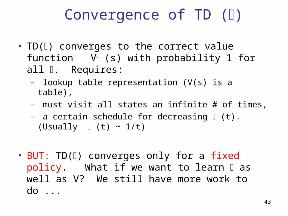
Convergence of TD ()

• TD() converges to the correct value function V (s) with probability 1 for all . Requires:– lookup table representation (V(s) is a table),– must visit all states an infinite # of times,– a certain schedule for decreasing (t).

(Usually (t) ~ 1/t)

• BUT: TD() converges only for a fixed policy. What if we want to learn as well as V? We still have more work to do ...

44

Q-Learning: TD Idea to Learn *

• Q-Learning (Watkins, 1989): one-step sample backup to learn action-value function Q(s,a). The most important RL algorithm in use today. Uses one-step error:

to define an incremental learning algorithm:

where (t) follows same schedule as in TD algorithm.

),(),'(max),( asQbsQraserrorb

),(),'(max),( asQbsQrasQ

b

Q-Learning Algorithmic Components

• Learning update (to Q-Table):

Q(s, a) (1-α)Q(s, a) + α[r + γ Q(s’, a’)]

or

Q(s, a) Q(s, a) + α[r + γ Q(s’, a’) - Q(s, a)]

• Action selection (from Q-Table):

a = f(Q(s, a))

a'

max

a'

max

a

argmax

Q-Learning Algorithm

46

47

Nice properties of Q-learning

• Q guaranteed to converge to Q* w/probability 1.

• Greedy guaranteed to converge to *.

• But (amazingly), don’t need to follow a fixed policy, or the greedy policy, during learning! Virtually any policy will do, as long as all (s,a) pairs visited infinitely often.

• As with TD, don’t need a model, can learn online, both bootstraps and samples.

),(maxarg)( asQsa

48

RL and Function Approximation

• DP infeasible for many real applications due to curse of dimensionality: |S| too big.

• FA may provide a way to “lift the curse:”– complexity D of FA needed to capture regularity in

environment may be << |S|.– no need to sweep thru entire state space: train on N

“plausible” samples and then generalize to similar samples drawn from the same distribution.

– PAC learning tells us generalization error ~D/N; N need only scale linearly with D.

49

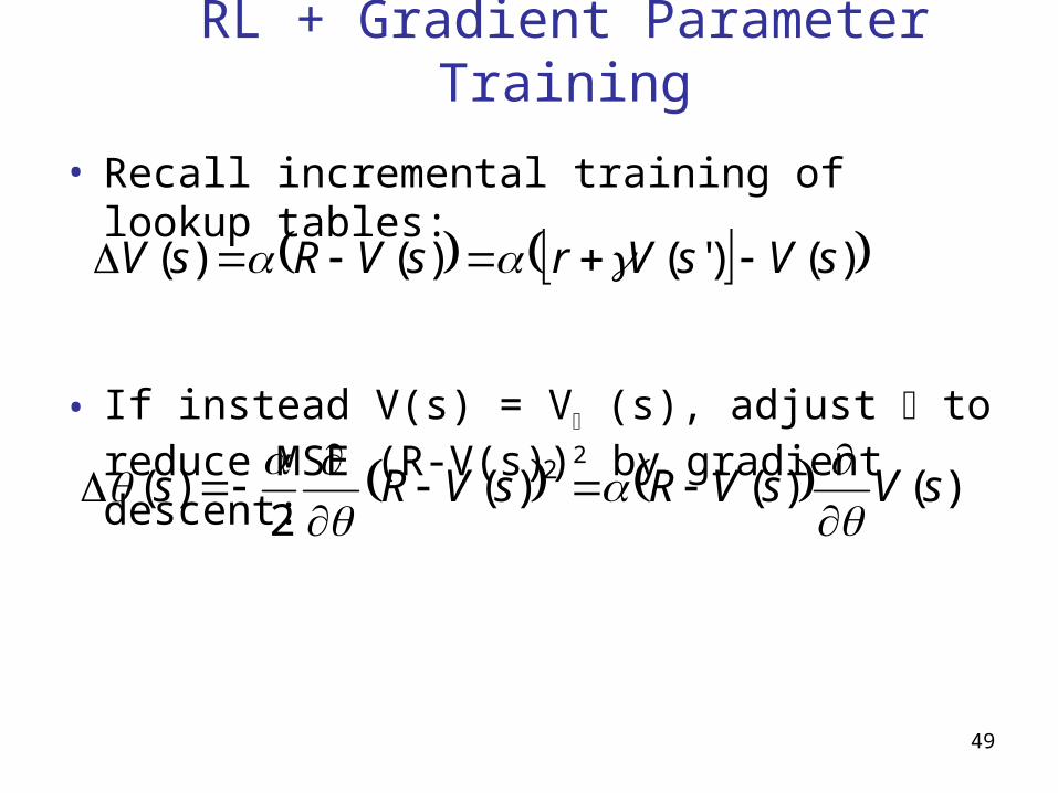
RL + Gradient Parameter Training

• Recall incremental training of lookup tables:

• If instead V(s) = V (s), adjust to reduce MSE (R-V(s))2 by gradient descent:

)()'()()( sVsVrsVRsV

)()()(2

)( 2 sVsVRsVRs

50

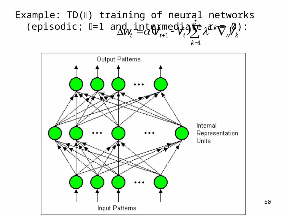
Example: TD() training of neural networks (episodic; =1 and intermediate r = 0):

kw

t

k

ktttt VVVw

11

51

Case-Study Applications

• Several commonalities:– Problems are more-or-less MDPs– |S| is enormous can’t do DP– State-space representation critical: use of

“features” based on domain knowledge– FA is reasonably simple (linear or NN)– Train in a simulator! Need lots of

experience, but still << |S|– Only visit plausible states; only generalize to

plausible states

52

47

53

Learning backgammon using TD()

• Neural net observes a sequence of input patterns x1, x2, x3, …, xf : sequence of board positions occurring during a game

• Representation: Raw board description (# of White or Black checkers at each location) using simple truncated unary encoding. (“hand-crafted features” added in later versions)

• At final position xf, reward signal z given:

– z = 1 if White wins;– z = 0 if Black wins

• Train neural net using gradient version of TD()• Trained NN output Vt = V (xt , w) should estimate

prob (White wins | xt )

54

49

55

Q: Who makes the moves??

• A: Let neural net make the moves itself, using its current evaluator: score all legal moves, and pick max Vt for White, or min Vt for Black.

• Hopelessly non-theoretical and crazy:– Training V using non-stationary (no convergence proof)– Training V using nonlinear func. approx. (no cvg. proof)– Random initial weights Random initial play! Extremely long

sequence of random moves and random outcome Learning seems hopeless to a human observer

• But what the heck, let’s just try and see what happens...

56

• TD-Gammon can teach itself by playing games against itself and learning from the outcome– Works even starting from random initial play and zero initial expert

knowledge (surprising!) achieves strong intermediate play– add hand-crafted features: advanced level of play (1991) – 2-ply search: strong master play (1993)– 3-ply search: superhuman play (1998)

• “TD-Leaf:” n-step TD backups in 2-player

• games (Beal; Baxter et al.): great results• for checkers and chess

57

RL Success Stories/Videos

• U. Michigan RL wiki page:– “keep-away” in Robocup simulator– Aibo fast walk gate; ball acquisition– Humanoid robot Air hockey– Helicopter aerobatics (Ng et al.)

• Human flies helicopter for 10-20 mins• Perform System Identification: learn model of

helicopter dynamics• Using model, train RL policy in simulator

58

Cell-phone channel allocation

S. Singh and D. Bertsekas, NIPS-96• Dynamic resource allocation: assign channels to calls in

a cell; can’t interfere with neighboring cell

• Problem is a real-time discrete-event MDP with huge state space ~ 7049 states

• Objective: maximize:

0

)( dttCeEV t

59

Modified Bellman optimality equation

Modify equation to handle continuous time, discrete events:

where: s = configuration, e=random event (arrival, handoff, departure) a=action, t=random time to next event, c(s,a, t) = effective immediate payoff

)'()(),,(max)( *

),(

* sVttascEEsV tesAa

e

60

• represent sx using 2 features for each cell:– Availability: # of free channels in a cell– Cell-channel packing: # of times channel is used in 4-cell radius

• represent V using linear FA: V = x• train in simulator using gradient version of TD(0)

xxVxVttaxc )()'()(),,(

54

61

RL training results (BDCL=best prev. algo.)

55

62

56

63

57

64

58

65

59

66

60

67

61

68

62

69

63

70

64

71

RL for Spoken Dialogue Systems

• Singh, Litman, Kearns, Walker (JAIR 2002)• Sequence of human-computer speech interactions• Use in DB-query system “NJFun:” database of leisure activities in

NJ, organized by (type, location, time)• Humans aren’t MDPs, but pretend they are: devise MDP

representation of system-human interaction:

72

• Severely restrict state space: 7 state variables and 42 “choice-state” combinations

73

• Severely restrict the policy: 2 actions possible in each choice-state: 242 possible policies; train using random exploration

• Actions are spoken requests to the user, classified as:– system initiative: “Please state the type of activity you are interested in”

– user initative: “How may I help you?”

– mixed initiative: “Please say the location you are interested in. You can also tell me the time.”

– confirmation of an attribute: “Did you say you are interested in going to a museum?”

• Train on a corpus of 311 dialogues (using AT&T volunteers); test trained system on 124 test dialogues. “Reward” after each dialogue is both objective (was the specific task completed exactly or partially) as well as subjective (“good,” “bad,” or “so-so” performance) from the human

• Small MDP but don’t have a model! Do Q-Learning using sample trajectories with the above random-exploration policy

74

• Results: Learned policy much better than random exploration

75

• Results: Learned policy much better than standard policies

76

70

77

RL Mashups

• RL + semi-supervised learning• RL + active learning• RL + metric learning• RL + dimensionality reduction• Bayesian RL• RL + SVMs/kernel methods• RL + semi-definite programming• RL + Gaussian process models• etc. etc.

• NIPS 2006 workshop “Towards A New Reinforcement Learning:” www.jan-peters.net/Research/NIPS2006

78

Final remarks on RL

• Can solve MDPs on-line, in real environment, without knowing underlying MDP

• Function Approximators can avoid the “curse of dimensionality”

• Beyond MDPs: active research in RL for: – high-level planning,– structured (e.g. factored, hierarchical) MDPs,– partially observable MDPs (POMDPs), – history dependent problems, – non-stationary problems, – multi-agent problems

• For more info, go to: RichSutton.com

79

Game Theory and Multi-Agent Learning

80

Outline

Description of the problem

Tools and concepts from RL & game theory

“Naïve” approaches to multi-agent learning

ordinary single-agent RL

evolutionary game theory

“Sophisticated” approaches

minimax-Q, FriendOrFoe-Q (Littman),

tinkering with learning rates: WoLF (Bowling), “strategic teaching” (Camerer)

Challenges and Opportunities

81

Normal single-agent learning

• Assume that environment has observable states, characterizable expected rewards and state transitions, and all of the above is stationary (MDP-ish)

• Non-learning, theoretical solution to fully specified problem: DP formalism

• Learning: solve by trial and error without a full specification: RL + exploration, Monte Carlo, ...

82

Multi-Agent Learning Problem:

• Agent tries to solve its learning problem, while other agents in the environment also are trying to solve their own learning problems. challenging non-stationarity.

• Main scenarios: (1) cooperative; (2) self-interest (many deep issues swept under the rug)

• Agent may know very little about other agents:– payoffs may be unknown– learning algorithms unknown

• Traditional method of solution: game theory (uses several questionable assumptions)

83

MAL needs foundational principles!

• A precise problem formulation is still lacking! See: “If Multi-Agent Learning is the Answer, What is the Question?” Shoham et al, 2006

• Some (debatable) MAL objectives:– Learning should converge to a stationary strategy– In “self-play” learning (all agents use same learning algorithm),

learners should jointly converge to an equilibrium strategy– Learning should achieve payoffs as good as a best-response to

other agents’ strategies– (Worst case bound) Learning should guarantee a minimum

payoff (“security payment,” “no-regret” property)

84

Game Theory

Provides essential theoretical/conceptual background for tackling multi-agent learning

Wikipedia definition:Game theory is most often described as a branch of

applied mathematics and economics that studies situations where players choose different actions in an attempt to maximize their returns. The essential feature, however, is that it provides a formal modelling approach to social situations in which decision makers interact with other minds.

Today, widely used in politics, business, economics, biology, psychology, computer science etc.

85

Fundamental Postulate of Game Theory: “Rationality”

• A rational player/agent will make decisions that maximize her individual expected utility (= expected payoff for simplicity) given her understanding/beliefs about the problem. Also, perfectly indifferent to payoffs received by other players.

86

Basics of game theory

• A game is specified by: players (1…N), actions, and (expected) payoff matrices (functions of joint actions)

B’s action

A’s action

A’s payoff B’s payoff

• If payoff matrices are identical, A and B are cooperative, else non-cooperative (zero-sum = purely competitive)

011

101

110

S

P

R

SPR

011

101

110

S

P

R

SPR

87

Basic lingo…(2)

• Games with no states: (bi)-matrix games• Games with states: stochastic games, Markov games;

(state transitions are functions of joint actions)

• Games with simultaneous moves: normal form• Games with alternating turns: extensive form

• No. of rounds = 1: one-shot game• No. of rounds > 1: repeated game

• deterministic action policy: pure strategy• non-deterministic action policy: mixed strategy

e.g. Prob(R,P,S) = (½,¼,¼)

88

Stochastic vs. Matrix Games

• A stochastic game (a.k.a. “Markov game” ) generalizes MDPs to multiple agents– finite state space S– joint action set– stationary reward distribution– stationary transition probabilities

• A matrix game has no state information, only joint actions and payoffs (|S| = 1)

)a(s

a),(sria),( s|s'P

89

Basic Analysis

• Agent i’s mixed strategy xi is a best-response to others’ x-i if it maximizes payoff given x-i

• xi is a dominant strategy if it maximizes payoff regardless of what others do

• A joint strategy x is an equilibrium if each agent’s strategy is simultaneously a best-response to everyone else’s strategy, i.e. no incentive to deviate. Nash equilibrium is the main one, but there are others (e.g. correlated equilibrium)

• A Nash equilibrium always exists, but may be exponentially many of them, and very hard to compute

equilibrium coordination (players agree on which eqm to choose) is a big problem

90

What about imperfect information games?

• Nash eqm. requires full observability of all game info. For imperfect info. games (e.g. each player has private info), corresponding concept is Bayes-Nash equilibrium (Nash plus Bayesian inference over hidden information). Even more intractable than regular Nash.

91

Pros and Cons of game theory

• Game theory provides a basic conceptual/theoretical framework for thinking about multi-agent learning.

• Game theory is appropriate provided that:– Game is stationary and fully specified; X– Enough computer power to compute equilibrium; X– Can assume other agents are also game theorists; X– Can solve equilibrium coordination problem. X

• Above conditions rarely hold in real applications Multi-agent learning is not only a fascinating problem,

it may be the only viable option.

92

Real-Life vs. Game Theory games

• NFL playoffs• World Series of Poker• World of Warcraft• Buying a house• Salary negotiations• Competitive pricing:

– Best Buy vs. Circuit City– Airline fare wars

• OPEC production cuts• NASDAQ, NYSE, …• FCC spectrum auctions

• Matching Pennies• Rock-Paper-Scissors• Prisoners’ Dilemma• Battle-of-the-Sexes• Chicken• Ultimatum

93

Assumptions in Normal-Form Games

• Game specification is fully known; actions and payoffs are fully observable by all players

• Players act “simultaneously”, i.e. without observing actions of others (not scalable!)

• Assume no communication between players, or it doesn’t affect play (communication is “cheap talk”)

• Basic analysis assumes the game is only played once (called one-shot)

94

Presentation of Rock Paper Scissors Payoffs in a Bimatrix

This is a zero-sum game since for each pair of joint actions, the players’ payoffs add up to zero.

This is a symmetric game: invariant under swapping of player labels

This game has a unique mixed strategy Nash equilibrium: both players play uniform random strategies: prob(R,P,S)=(1/3,1/3,1/3)

Column player

R P S

R 0

0

-1

+1

+1

-1

Row player

P +1

-1

0

0

-1

+1

S -1

+1

+1

-1

0

0

95

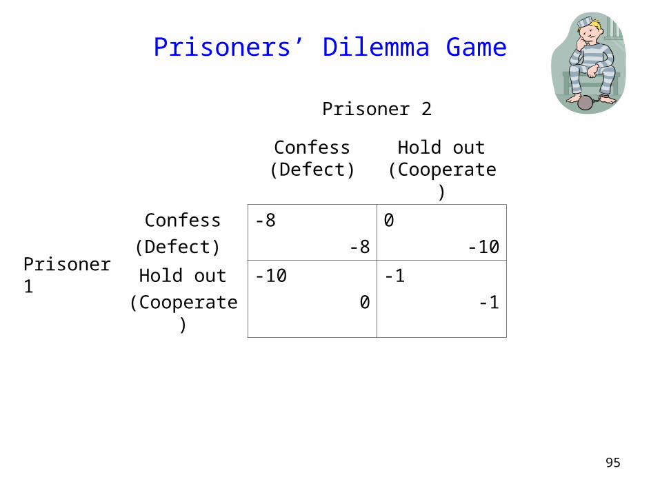
Prisoners’ Dilemma Game

Prisoner 2

Confess (Defect)

Hold out (Cooperate)

Prisoner 1

Confess

(Defect)

-8

-8

0

-10

Hold out

(Cooperate)

-10

0

-1

-1

96

Prisoners’ Dilemma Game

Prisoner 2

Confess (Defect)

Hold out (Cooperate)

Prisoner 1

Confess

(Defect)

-8

-8

0

-10

Hold out

(Cooperate)

-10

0

-1

-1

Whatever Prisoner 2 does, the best that Prisoner 1 can do is Confess

97

Prisoners’ Dilemma Game

Prisoner 2

Confess (Defect)

Hold out (Cooperate)

Prisoner 1

Confess

(Defect)

-8

-8

0

-10

Hold out

(Cooperate)

-10

0

-1

-1

Whatever Prisoner 1 does, the best that Prisoner 2 can do is Confess.

98

Prisoners’ Dilemma Game

Prisoner 2

Confess (Defect)

Hold out (Cooperate)

Prisoner 1

Confess

(Defect)

-8

-8

0

-10

Hold out

(Cooperate)

-10

0

-1

-1

A strategy is a dominant strategy if it is a player’s strictly best response to any strategies the other players might pick.

A dominant strategy equilibrium is a strategy combination consisting of each players dominant strategy.

Each player has a dominant strategy to Confess.

The dominant strategy equilibrium is (Confess,Confess)

99

Prisoners’ Dilemma Game

Prisoner 2

Confess (Defect)

Hold out (Cooperate)

Prisoner 1

Confess

(Defect)

-8

-8

0

-10

Hold out

(Cooperate)

-10

0

-1

-1

The payoff in the dominant strategy equilibrium (-8,-8) is worse for both players than (-1,-1), the payoff in the case that both players hold out. Thus, the Prisoners’ Dilemma Game is a game of social conflict.

Opportunity for multi-agent learning: by learning during repeated play, the Pareto optimal solution (-1,-1) can emerge as a result of learning (also can arise in evolutionary game theory).

100

Battle of the Sexes

Bob

Prize Fight Ballet

Alice

Prize fight 2

1

-1

-1

Ballet -5

-5

1

2

101

Battle of the Sexes

Bob

Prize Fight Ballet

Alice

Prize fight 2

1

-1

-1

Ballet -5

-5

1

2

This game has

no (iterated) dominant strategy equilibrium

102

Battle of the Sexes

Bob

Prize Fight Ballet

Alice

Prize fight 2

1

-1

-1

Ballet -5

-5

1

2

This game has

no (iterated) dominant strategy equilibrium

103

Battle of the Sexes

Bob

Prize Fight Ballet

Alice

Prize fight 2

1

-1

-1

Ballet -5

-5

1

2

This game has

no (iterated) dominant strategy equilibrium

two Nash equilibria (Prize Fight, Prize Fight) and (Ballet, Ballet)

104

Battle of the Sexes

Bob

Prize Fight Ballet

Alice

Prize fight 2

1

-1

-1

Ballet -5

-5

1

2

This game has two Nash equilibria

How can these two players coordinate ?

105

Multiagent Q-learning desiderata

“performs well” vs. arbitrarily adapting other agents best-response probably impossible

Doesn’t need correct model of other agents’ learning algorithms

But modeling is fair game

Doesn’t need to know other agents’ payoffs

Estimate other agents’ strategies from observation do not assume game-theoretic play

No assumption of stationary outcome: population may never reach eqm, agents may never stop adapting

Self-play: convergence to repeated Nash would be nice but not necessary. (unreasonable to seek convergence to a one-shot Nash)

106

Naïve Approaches to Multi-Agent Learning

• Basic idea: agent adapts, ignoring non-stationarity of other agents’ strategies

• 1. Evolutionary game theory: “Replicator Dynamics” models: large population of agents using different strategies, fittest agents breed more copies.

– Let x= population strategy vector, and xk = fraction of population playing strategy k. Growth rate then:

– Above eqn also derived from an “imitation” model– NE are fixed points of above equation, but not

necessarily attractors (unstable or neutral stable)

),(),( xxuxeuxdt

dx kk

k

107

Many possible dynamic behaviors...

• limit cycles attractors unstable f.p.

• Also saddle points, chaotic orbits, ...

108

Replicator dynamics: auction bidding strategies

109

More Naïve Approaches…

• 2. Iterated Gradient Ascent: (Singh, Kearns and Mansour): Again does a myopic adaptation to other players’ current strategy.

– Coupled system of linear equations: u is linear in x i and x-i

– Analysis for two-player, two-action games: either converges to a Nash fixed point on the boundary (at least one pure strategy), or get limit cycles

),( iii

i xxuxdt

dx

110

Further Naïve Approaches…

• 3. Dumb Single-Agent Learning: Use a single-agent algorithm in a multi-agent problem & hope that it works

– No-regret learning by pricebots (Greenwald & Kephart)– Simultaneous Q-learning by pricebots (Tesauro & Kephart)

– In many cases, this actually works: learners converge either exactly or approximately to self-consistent optimal strategies

• Naïve approaches are “rational” i.e. they converge to a best response against a stationary opponent– but they generally don’t converge to Nash equilibrium

111

A Fancier Approach

• 4. No-regret learning: (Hart & Mas-Colell, Freund & Schapire, many others): Define regret for playing a sequence si instead of constant action aj for t time steps:

– Then choose next action with probability proportional to:

• prob (action j) ~

– This has a worst-case guarantee that asymptotic regret per time step 0, i.e., will be as good as best (constant) action choice

t

k

k

i

k

i

t

i

k

ij

t

iiij

t

i ssRsaRssar1

,,|,

0),,(max ijti sar

112

“Sophisticated” approaches

• Takes into account the possibility that other agents’ strategies might change.

• 4. Equilibrium Q-learners:

– Minimax-Q (Littman): converges to Nash equilibrium for two-player zero-sum stochastic games

– FriendOrFoe-Q (Littman): convergent algorithm for games where every other player can be identified as “friend” (same payoffs as me) or “foe” (payoffs are zero-sum)

• These algorithms converge to Nash equilibrium but aren’t “rational” since they don’t best-respond to a fixed opponent

113

More sophisticated approaches...

• 5. Varying learning rates

– WoLF: “Win or Learn Fast” (Bowling): agent reduces its learning rate when performing well, and increases when doing badly. Improves convergence of IGA and policy hill-climbing

– GIGA-WoLF (Bowling): Combines the IGA algorithm with WoLF idea. Provably convergent + no-regret.

114

More sophisticated approaches...

• 6. “Strategic Teaching:” recognizes that other players’ strategy are adaptive

– “A strategic teacher may play a strategy which is not myopically optimal (such as cooperating in Prisoner’s Dilemma) in the hope that it induces adaptive players to expect that strategy in the future, which triggers a best-response that benefits the teacher.” (Camerer, Ho and Chong)

115

Theoretical Research Challenges

• Proper theoretical formulation?– “No short-cut” hypothesis: Massive on-line search a la

Deep Blue to maximize expected long-term reward– (Bayesian) Model and predict behavior of other players,

including how they learn based on my actions (beware of infinite model recursion)

– trial-and-error exploration– continual Bayesian inference using all evidence over all

uncertainties (Boutilier: Bayesian exploration)• When can you get away with simpler methods?

116

Real-World Opportunities

• Multi-agent systems where you can’t do game theory (covers everything :-))– Electronic marketplaces – Mobile networks – Self-managing computer systems– Teams of robots– Video games – Military/counter-terrorism applications

117

Backup Slides