1

Introduction

The temporal behavior of systems, such as e.g. technical systems from the areas ofelectrical engineering, mechanical engineering, and process engineering, as well asnon-technical systems from areas as diverse as biology, medicine, chemistry, physics,economics, to name a few, can uniformly be described by mathematical models. Thisis covered by systems theory. However, the application of systems theory requiresthat the mathematical models for the static and dynamic behavior of the systemsand their elements are known. The process of setting up a suitable model is calledmodeling. As is shown in the following section, two general approaches to model-ing exist, namely theoretical and experimental modeling, both of which have theirdistinct advantages and disadvantages.

1.1 Theoretical and Experimental Modeling

A system is understood as a confined arrangement of mutually affected entities, seee.g. DIN 66201. In the following, these entities are processes. A process is definedas the conversion and/or the transport of material, energy, and/or information. Here,one typically differentiates between individual (sub-)processes and the entire pro-cess. Individual processes, i.e. (sub-)processes, can be the generation of mechanicalenergy from electric energy, the metal-cutting machining of workpieces, heat trans-fer through a wall, or a chemical reaction. Together with other sub-processes, theentire process is formed. Such aggregate processes can be an electrical generator, amachine tool, a heat exchanger, or a chemical reactor. If such a process is understoodas an entity (as mentioned above), then multiple processes form a system such as e.g.a power plant, a factory, a heating system, or a plastic material production plant. Thebehavior of a system is hence defined by the behavior of its processes.

The derivation of mathematical system and process models and the representa-tion of their temporal behavior based on measured signals is termed system analysisrespectively process analysis. Accordingly, one can speak of system identificationor process identification when applying the experimental system or process analy-sis techniques described in this book. If the system is excited by a stochastic signal,

R. Isermann, M. Münchhof, Identification of Dynamic Systems, DOI 10.1007/978-3-540-78879-9_1, © Springer-Verlag Berlin Heidelberg 2011

2 1 Introduction

A-priori Knowledgeabout System

Identification

Experimental Model

StructureKnown

Parametric

ParametricStructureStructure

ParametersParameters

Simplifying Assumptions

Simplification

Comparison

Resulting Model

Experiment

Physical Laws

Theoretical Model

Simplified Theoretical Model

1) Balance Equations2) Constitutive Equations3) Phenomenological Equations4) Interconnection Equations

1) Structure2) Parameters

Theoretical Modeling Experimental Modeling

StructureUnknown

Non-Parametric

Non-Parametric

Case ACase B

B/1

A/2

A/1

Fig. 1.1. Basic procedure for system analysis

one also has to analyze the signal itself. Thus the topic of signal analysis will alsobe treated. The title Identification of Dynamic Systems or simply Identification shallthus embrace all areas of identification as listed above.

For the derivation of mathematical models of dynamic systems, one typically dis-criminates between theoretical and experimental modeling. In the following, the ba-sic approach of the two different ways of modeling shall be described shortly. Here,one has to distinguish lumped parameter systems and distributed parameter systems.

1.1 Theoretical and Experimental Modeling 3

The states of distributed parameter systems depend on both the time and the locationand thus their behavior has to be described by partial differential equations (PDEs).Lumped parameter systems are easier to examine since one can treat all storages andstates as being concentrated in single points and not spatially distributed. In this case,one will obtain ordinary differential equations (ODEs).

For the theoretical analysis, also termed theoretical modeling, the model is ob-tained by applying methods from calculus to equations as e.g. derived from physics.One typically has to apply simplifying assumptions concerning the system and/orprocess, as only this will make the mathematical treatment feasible in most cases. Ingeneral, the following types of equations are combined to build the model, see alsoFig. 1.1 (Isermann, 2005):

1. Balance equations: Balance of mass, energy, momentum. For distributed param-eter systems, one typically considers infinitesimally small elements, for lumpedparameter systems, a larger (confined) element is considered

2. Physical or chemical equations of state: These are the so-called constitutiveequations and describe reversible events, such as e.g. inductance or the secondNewtonian postulate

3. Phenomenological equations: Describing irreversible events, such as friction andheat transfer. An entropy balance can be set up if multiple irreversible processesare present

4. Interconnection equations according to e.g. Kirchhoff’s node and mesh equa-tions, torque balance, etc.

By applying these equations, one obtains a set of ordinary or partial differentialequations, which finally leads to a theoretical model with a certain structure and de-fined parameters if all equations can be solved explicitly. In many cases, the modelis too complex or too complicated, so that it needs to be simplified to be suitablefor subsequent application. Figure 1.2 shows the order of the execution of individ-ual simplifying actions. The first steps of this simplification procedure can alreadybe carried out as the fundamental equations are set up by making appropriate sim-plifying assumptions. It is very tempting to include as many physical effects intothe model as possible, especially nowadays, where simulation programs offer a widevariety of pre-build libraries of arbitrary degrees of complexity. However, this oftenoccludes the predominant physical effects and makes both the understanding and thework with such a model a very tiresome, if not infeasible, endeavor.

But even if the resulting set of equations cannot be solved explicitly, still theindividual equations give important hints concerning the model structure. Balanceequations are always linear, some phenomenological equations are linear in a widerange. The physical and chemical equations of state often introduce non-linearitiesinto the system model.

In case of an experimental analysis, which is also termed identification, a mathe-matical model is derived from measurements. Here, one typically has to rely on cer-tain a priori assumptions, which can either stem from theoretical analysis or fromprevious (initial) experiments, see Fig. 1.1. Measurements are carried out and the in-put as well as the output signals are subjected to some identification method in order

4 1 Introduction

Partial Differential Equationnon-linear

Partial Differential Equationlinear

Ordinary Differential Equationlinear, order n

Ordinary Differential Equationlinear, order < n

Algebraic Equationlinear

Ordinary Differential Equationnon-linear, order n

Ordinary Differential Equationnon-linear, order < n

Algebraic Equationnon-linear

Entry Points for Model Development

Linearize

Linearize

Approximation withLumped Parameters

Approximation withLumped Parameters

OrderReduction

OrderReduction

Set Time-Deri-vatives to Zero

Set Time-Deri-vatives to Zero

Fig. 1.2. Basic approach for theoretical modeling

to find a mathematical model that describes the relation between the input and theoutput. The input signals can either be a section of the the natural signals that acton the process during normal operation or can be an artificially introduced test sig-nal with certain prespecified properties. Depending on the application, one can useparametric or non-parametric models, see Sect. 1.2. The resulting model is termedexperimental model.

The theoretically and the experimentally derived models can be compared if bothapproaches can be applied and have been pursued. If the two models do not match,then one can get hints from the character and the size of the deviation, which stepsof the theoretical or the experimental modeling have to be corrected, see Fig. 1.1.

Theoretical and experimental models thus complement one another. The analysisof the two models introduces a first feedback loop into the course of action for systemanalysis. Therefore, system analysis is typically an iterative procedure. If one is notinterested in obtaining both models simultaneously, one has the choice between theexperimental model (case A in Fig. 1.1) and the theoretical model (case B in Fig. 1.1).The choice mainly depends on the purpose of the derived model:

The theoretical model contains the functional dependencies between the physicalproperties of a system and its parameters. Thus, this model will typically be preferredif the system shall already be optimized in its static and dynamic behavior during the

1.1 Theoretical and Experimental Modeling 5

design phase or if its temporal behavior shall be simulated prior to the construction,respectively completion of the system.

On the contrary, the experimental model does only contain numbers as para-meters, whose functional relations to the process properties remain unknown. How-ever, this model can describe the actual dynamics of the system better and can bederived with less effort. One favors these experimental models for the adaptation ofcontrollers (Isermann, 1991; Isermann et al, 1992; Åström et al, 1995; Åström andWittenmark, 1997) and for the forecast of the respective signals or fault detection (Is-ermann, 2006).

In case B (Fig. 1.1), the main focus is on the theoretical analysis. In this set-ting, one employs the experimental modeling only once to validate the fidelity ofthe theoretical model or to determine process parameters, which can otherwise notbe determined with the required accuracy. This is noted with the sequence B/1 inFig. 1.1.

In contrast to case B, the emphasis is on the experimental analysis in case A.Here, one tries to apply as much a priori knowledge as possible from the theoreticalanalysis, as the model fidelity of the experimental model normally increases withthe amount of a priori knowledge exploited. In the ideal case, the model structure isalready known from the theoretical analysis (path A/2 in Fig. 1.1). If the fundamentalequations of the model cannot be solved explicitly, if they are too complicated, or ifthey are not even completely known, one can still try to obtain information about themodel structure from this incomplete knowledge about the process (sequence A/1 inFig. 1.1).

The preceding paragraphs already pointed out that the system analysis can typi-cally neither be completely theoretical nor completely experimental. To benefit fromthe advantages of both approaches, one does rarely use only theoretical modeling(leading to so-called white-box models) or only experimental modeling (leading toso-called black-box models), but rather a mixture of both leading to what is calledgray-box models, see Fig. 1.3. This is a rather suitable combination of the two ap-proaches, which is determined by the scope of application of the model and the sys-tem itself. The scope of application defines the required model accuracy and hencethe effort that has to be put into the analysis. This introduces a second feedback loopinto the schematic diagram presented in Fig. 1.1, which starts at the resulting models(either theoretical or experimental) and goes back to the individual modeling steps,hence one is confronted with a second iteration loop.

Despite the fact that the theoretical analysis can in principle deliver more infor-mation about the system, provided that the internal behavior is known and can bedescribed mathematically, experimental analysis has found ever increasing attentionover the past 50 years. The main reasons are the following:

� Theoretical analysis can become quite complex even for simple systems� Mostly, model coefficients derived from the theoretical considerations are not

precise enough� Not all actions taking place inside the system are known

6 1 Introduction

Theoreticalmodeling

Experimentalmodeling

�

�

Physical lawsknownParameters known

�

�

PhysicallawsknownPara-metersun-known

� Signalsmeasu-rable

�

�

�

PhysicalrulesknownModelstructureun-knownPara-metersun-known

� Signalsmeasu-rable

�

�

Input/outputsignals measurableAssumption of amodel structure

White-BoxModel

Light-Gray-BoxModel

Dark-Gray-BoxModel

Black-BoxModel

�Linear/non-lineardifferentialequations

�Differentialequations withparameterestimation

�Neuro/fuzzymodels withparameterestimation

�

�

Impulse responseNeural networks

Fig. 1.3. Different kinds of mathematical models ranging from white box models to black boxmodels

� The actions taking place cannot be described mathematically with the requiredaccuracy

� Some systems are very complex, making the theoretical analysis too time-consuming

� Identified models can be obtained in shorter time with less effort compared totheoretical modeling

The experimental analysis allows the development of mathematical models bymeasurement of the input and output of systems of arbitrary composition. One majoradvantage is the fact that the same experimental analysis methods can be applied todiverse and arbitrarily complex systems. By measuring the input and output only,one does however only obtain models governing the input-output behavior of thesystem, i.e. the models will in general not describe the precise internal structure ofthe system. These input-output models are approximations and are still sufficient formany areas of application. If the system also allows the measurement of internalstates, one can obviously also gather information about the internal structure of the

1.2 Tasks and Problems for the Identification of Dynamic Systems 7

Table 1.1. Properties of theoretical modeling and identification

Theoretical Modeling Identification

Model structure follows from laws ofnature

Model structure must be assumed

Modeling of the input/output behavioras well as the internal behavior

Only the input/output behavior is iden-tified

Model parameters are given as functionof system properties

Model parameters are “numbers” only,in general no functional dependency tosystem properties known

Model is valid for the entire class ofprocesses of a certain type and for dif-ferent operating conditions

Model is only valid for investigated sys-tem and within operating limits

Model coefficients are not known ex-actly

Model coefficients are more precise forthe given system within operating limits

Models can be build for non-existingsystems

Model can only be identified for an ex-isting system

The internal behavior of the systemmust be known and must be describablemathematically

Identification methods are independentof the investigated system and can thusbe applied to many different systems

Typically lengthy process which takesup much time

Fast process if identification methodsexist already

Models may be rather complex and de-tailed

Model size can be adjusted according tothe area of application of the model

system. With the advent of digital computers starting in the 1960s, the developmentof capable identification methods has started. The different properties of theoreticalmodeling and identification have been summarized and set in contrast in Table 1.1.

1.2 Tasks and Problems for the Identification of Dynamic Systems

A process with a single input and a single output (SISO) is considered in the follow-ing. The process shall be stable to ensure a unique relation between input and output.Both the input and the output shall be measured without error. The task of identifyingthe process P is to find a mathematical model for the temporal behavior of the pro-cess from the measured input u.t/ D uM.t/, the measured output y.t/ D yM.t/ andoptionally additional measured signals, see Fig. 1.4. This task is made more com-plicated, if disturbances ´1 : : : ´i are acting on the process and are influencing theoutput signal. These disturbances can have various causes. The disturbances seen inthe measured signals often stem from noise and hence will also be included in theterm noise in the remainder of this book. The output is thus corrupted by a noisen.t/. In this case, one has to apply suitable techniques to separate the wanted signal

8 1 Introduction

Process P

z1 zi. . .

u y

u uM= y yM=

Process Pu y

u uM= y yM=

yu

yz

Fig. 1.4. Dynamic process with input u,output y and disturbances ´i

Fig. 1.5. Disturbed dynamic process withinput u, output y, and noise n

yu.t/, i.e. the response of the system due to the input u.t/, from the disturbancesn.t/.

The term identification and the required subsequent tasks can thus be defined asfollows:

Identification is the experimental determination of the temporal behavior of aprocess or system. One uses measured signals and determines the temporal behaviorwithin a class of mathematical models. The error (respectively deviation) betweenthe real process or system and its mathematical model shall be as small as possible.

This definition stems from Zadeh (1962), see also (Eykhoff, 1994). The measuredsignals are typically only the input to the system and the output from the system.However, if it is also possible to measure states of the process, then one can alsogather information about the internal structure of the process.

In the following, a linear process is considered. In this case, the individual distur-bance components ´1; : : : ; ´i can be combined into one representative disturbancen.t/, which is added to the wanted signal yu.t/, see Fig. 1.5. If this disturbance n.t/is not negligibly small, then its counterfeiting influence must be eliminated by theidentification method as much as possible. For decreasing signal-to-noise ratios, themeasurement time TM must typically be increased.

For the identification itself, the following limitations have to be taken into con-sideration:

1. The available measurement time TM is always limited, either due to technicalreasons, due to time variance of the process parameters or due to economicalreasons (i.e. budget), thus

TM � TM;max (1.2.1)

2. The maximum allowable change of the input signal, i.e. the test signal heightu0 is always limited, either due to technical reasons or due to the assumption oflinear process behavior which is only valid within a certain operating regime

umin � u.t/ � umax (1.2.2)

3. The maximum allowable change of the output signal, y0, may also be limiteddue to technical reasons or due to the assumption of linear process behavior

1.2 Tasks and Problems for the Identification of Dynamic Systems 9

a)

b)

c)

t

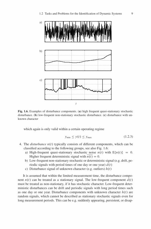
Fig. 1.6. Examples of disturbance components. (a) high frequent quasi-stationary stochasticdisturbance. (b) low-frequent non-stationary stochastic disturbance. (c) disturbance with un-known character

which again is only valid within a certain operating regime

ymin � y.t/ � ymax (1.2.3)

4. The disturbance n.t/ typically consists of different components, which can beclassified according to the following groups, see also Fig. 1.6:a) High-frequent quasi-stationary stochastic noise n.t/ with Efn.t/g D 0.

Higher frequent deterministic signal with n.t/ D 0.b) Low-frequent non-stationary stochastic or deterministic signal (e.g. drift, pe-

riodic signals with period times of one day or one year) d.t/c) Disturbance signal of unknown character (e.g. outliers) h.t/

It is assumed that within the limited measurement time, the disturbance compo-nent n.t/ can be treated as a stationary signal. The low-frequent component d.t/must be treated as non-stationary, if it has stochastic character. Low-frequent deter-ministic disturbances can be drift and periodic signals with long period times suchas one day or one year. Disturbance components with unknown character h.t/ arerandom signals, which cannot be described as stationary stochastic signals even forlong measurement periods. This can be e.g. suddenly appearing, persistent, or disap-

10 1 Introduction

pearing disturbances and so-called outliers. These disturbances can e.g. stem fromelectromagnetic induction or malfunctions of the measurement equipment.

Typical identification methods can only eliminate the noise n.t/ as the measure-ment time is prolonged. Simple averaging or regression methods are often sufficientin this application. The components d.t/ require more specifically tailored measuressuch as special filters or regression methods which have been adapted to the veryparticular type of disturbance. Almost no general hints can be given concerning theelimination of the influence of h.t/. Such disturbances can only be eliminated man-ually or by special filters.

Effective identification methods must thus be able to determine the temporal be-havior as precisely as possible under the constraints imposed by

� the given disturbance yz.t/ D n.t/C d.t/C h.t/

� the limited measurement time TM � TM;max� the confined test signal amplitude umin � u.t/ � umax� the constrained output signal amplitude ymin � y.t/ � ymax� the purpose of the identification.

Figure 1.7 shows a general sequence of an identification. The following stepshave to be taken:

First, the purpose has to be defined as the purpose determines the type of model,the required accuracy, the suitable identification methods and such. This decisionis typically also influenced by the available budget, either the allocated financialresources or the expendable time.

Then, a priori knowledge must be collected, which encompasses all readily avail-able information about the process to be identified, such as e.g.

� recently observed behavior of the process� physical laws governing the process behavior� rough models from previous experiments� hints concerning linear/non-linear, time-variant/time-invariant as well as propor-

tional/integral behavior of the process� settling time� dead time� amplitude and frequency spectrum of noise� operating conditions for conduction of measurements.

Now, the measurement can be planned depending on the purpose and the avail-able a priori knowledge. One has to select and define the

� input signals (normal operating signals or artificial test signals and their shape,amplitude and frequency spectrum)

� sampling time� measurement time� measurements in closed-loop or open-loop operation of the process� online or offline identification� real-time or not

1.2 Tasks and Problems for the Identification of Dynamic Systems 11

Fundamental Physical EquationsInitial Experiments

Operating ConditionsTask

Budget

Purpose

Planning ofMeasurements

Signal GenerationMeasurementResults

Data Inspectionand Preprocessing

Application ofIdentification Method

Assumption ofModel Structure

Determination ofModel Structure

Model Vali-dation

Process Model

A-Priori Knowledge

ParametricNon-Para-metric

ResultingModel

Yes

No

Fig. 1.7. Basic sequence of the identification

12 1 Introduction

� necessary equipment (e.g. oscilloscope, PC, ...)� filtering for elimination of noise� limitations imposed by the actuators (saturation, ...).

Once these points have been clarified, the measurements can be conducted. Thisincludes the signal generation, measurement, and data storage.

The collected data should undergo a first visual inspection and outliers as wellas other easily detectable measurement errors should be removed. Then, as part ofthe further pre-processing, derivatives should be calculated, signals be calibrated,high-frequent noise be eliminated by e.g. low-pass filtering, and drift be removed.Some aspects of disturbance rejection and the removal of outliers by graphical andanalytical methods are presented in Chap. 23. Methods to calculate the derivativesfrom noisy measurements are shown in Chap. 15.

After that, the measurements will be evaluated by the application of identificationtechniques and determination of model structure.

A very important step is the performance evaluation of the identified model, theso-called validation by comparison of model output and plant output or comparisonof the experimentally established with the theoretically derived model. Validationmethods are covered in Chap. 23. Typically, an identified model with the necessarymodel fidelity will not be derived in the first iteration. Thus, additional iteration stepsmight have to be carried out to obtain a suitable model.

Therefore, the last step is the possible iteration, i.e. the repeated conduction ofmeasurements and evaluation of the measurements until a model meeting the im-posed requirements has been found. One often has to conduct initial experiments,which allow to prepare and conduct the main experiments with better suited para-meters or methods.

1.3 Taxonomy of Identification Methods and Their Treatment in ThisBook

According to the definition of identification as presented in the last section, the dif-ferent identification methods can be classified according to the following criteria:

� Class of mathematical model� Class of employed test signals� Calculation of error between process and model

It has proven practical to also include the following two criteria:

� Execution of experiment and evaluation (online, offline)� Employed algorithm for data processing

Mathematical models which describe the dynamic behavior of processes can begiven either as functions relating the input and the output or as functions relatinginternal states. They can furthermore be set up as analytical models in the form ofmathematical equations or as tables or characteristic curves. In the former case, the

1.3 Taxonomy of Identification Methods and Their Treatment in This Book 13

P P

P

M M-1

M1

u u

u

y y

y

n n

n

e

yM yM

+

-

Output Error Input Error

Generalized Equation Error

e +

-

M2

-1+-

e

Fig. 1.8. Different setups for calculating the error between model M and process P

parameters of the model are explicitly included in the equation, in the latter case, theyare not. Since the parameters of the system play a dominant role in identification,mathematical models shall first and foremost be classified by the model type as:

� Parametric models (i.e. models with structure and finite number of parameters)� Non-parametric models (i.e. models without specific structure and infinite num-

ber of parameters)

Parametric models are equations, which explicitly contain the process para-meters. Examples are differential equations or transfer functions given as an alge-braic expression. Non-parametric models provide a relation between a certain inputand the corresponding response by means of a table or sampled characteristic curve.Examples are impulse responses, step responses, or frequency responses presented intabular or graphical form. They implicitly contain the system parameters. Althoughone could understand the functional values of a step response as “parameters”, onewould however need an infinite number of parameters to fully describe the dynamicbehavior in this case. Consequently, the resulting model would be of infinite dimen-sion. In this book, parametric models are thus understood as models with a finitenumber of parameters. Both classes of models can be sub-divided by the type ofinput and output signals as continuous-time models or discrete-time models.

The input signals respectively test signals can be deterministic (analytically de-scribable) stochastic (random), or pseudo-stochastic (deterministic, but with proper-ties close to stochastic signals).

As a measure for the error between model and process, one can choose between(see Fig. 1.8) the following errors:

� Input error� Output error� Generalized equation error

14 1 Introduction

Process Process

DataStorage

DataStorage

Computer

Computer

Model

Model

Offline-Identification Online-Identification

Batch Processing Real-Time Processing

Non-Recursive Recursive

DirectProcessing

IterativeProcessing

Fig. 1.9. Different setups for the data processing as part of the identification

Because of mathematical reasons, typically those errors are preferred, which dependlinearly on the process parameters. Thus, one uses the output error if e.g. impulseresponses are used as models and the generalized equation error if e.g. differentialequations, difference equations, or transfer functions are employed. However, alsooutput errors are used in the last case.

If digital computers are utilized for the identification, then one differentiates be-tween two types of coupling between process and computer, see Fig. 1.9:

� Offline (indirect coupling)� Online (direct coupling)

For the offline identification, the measured data are first stored (e.g. data storage) andare later transferred to the computer utilized for data evaluation and are processedthere. The online identification is performed parallelly to the experiment. The com-

1.4 Overview of Identification Methods 15

puter is coupled with the process and the data points are operated on as they becomeavailable.

The identification with digital computers also allows to discern the identificationaccording to the type of algorithm employed:

� Batch processing� Real-time processing

In case of batch processing, the previously stored measurements will be processedin one shot, which is typically the case for offline applications. If the data are pro-cessed immediately after they become available, then one speaks of real-time pro-cessing, which necessitates a direct coupling between the computer and the process,see Fig. 1.9. Another feature is the processing of the data. Here, one can discern:

� Non-recursive processing� Recursive processing

The non-recursive methods determine the model from the previously stored measure-ments and are thus a method of choice for offline processing only. On the contrary,the recursive method updates the model as each measurement becomes available.Hence, the new measurement is always used to improve the model derived in theprevious step. The old measurements do not need to be stored. This is the typicalapproach for real-time processing and is called real-time identification. As not onlythe parameters, but also a measure of their accuracy (e.g. variance) can be calculatedonline, one can also think about running the measurement until a certain accuracy ofthe parameter estimates has been achieved (Åström and Eykhoff, 1971).

Finally, the non-recursive method can further be subdivided into:

� Direct processing� Iterative processing

The direct processing determines the model in one pass. The iterative processingdetermines the model step-wise. Thus, iteration cycles are emerging and the datamust be processed multiple times.

1.4 Overview of Identification Methods

The most important identification methods shall be described shortly. Table 1.2 com-pares their most prominent properties. A summary of the important advantages anddisadvantages of the individual methods can be found in Sect. 23.4.

1.4.1 Non-Parametric Models

Frequency response measurements with periodic test signals allow the direct deter-mination of discrete points of the frequency response characteristics for linear pro-cesses. The orthogonal correlation method has proven very effective for this task andis included in all frequency response measurement units. The necessary measurement

16 1 Introduction

Table 1.2. Overview of the most prominent identification methods

K

b+

bs

01

(1+

)Ts

n

G(j

)ω

n

G(j

)ω

n

g(t

) n

1+

as+

1

Par

amet

ric

No

n-P

aram

etri

c

No

n-P

aram

etri

c

No

n-P

aram

etri

c

Par

amet

ric

Met

ho

d

Det

erm

inat

ion

of

Ch

arac

teri

stic

Val

ues

Fo

uri

erA

nal

ysi

s

Fre

qu

ency

Res

po

nse

Mea

sure

men

t

Co

rrel

atio

nA

nal

ysi

s

Mo

del

Ad

just

men

t

Par

amet

erE

stim

atio

n

Inp

ut

Mo

del

Ou

tpu

t

All

ow

able

Sig

nal

-to

-N

ois

e ra

tio

mu

st b

e v

ery

larg

e

mu

st b

e la

rge

aver

age

can

be

smal

l

can

be

smal

l

mu

st b

e la

rge

OnlineProcessing

OfflineProcessing

BatchProcessing

Real-TimeProcessing

Time-VariantSystems

MIMOSystems

Res

ult

ing

Mo

del

Fid

elit

yS

cop

e o

fA

pp

lica

tio

n

� - � �

� � � �

� � � �

�-�

--

��

�

��

�-

Av

erag

e

Av

erag

e

Ver

y g

oo

d

Go

od

Av

erag

e

Go

od

� �

Ro

ug

h m

od

elC

on

tro

ller

tu

nin

g

�V

alid

atio

n o

f th

eore

tica

lly

der

ived

mo

del

s

�V

alid

atio

n o

f th

eore

tica

lly

der

ived

mo

del

s�

Des

ign

of

clas

sica

l (l

inea

r)co

ntr

oll

ers

�D

eter

min

atio

n o

f si

gn

al r

elat

ion

s�

Det

erm

inat

ion

of

tim

e d

elay

s

�D

esig

n o

f ad

apti

ve

con

tro

ller

s� �

Ad

apti

ve

con

tro

ller

sF

ault

det

ecti

on

�P

aram

eter

izat

ion

of

mo

del

s

LinearProcess

NonlinearProcess

�-

�-

�-

�-

� �

� �

��

�=

Ap

pli

cab

le;

- =

No

t ap

pli

cab

le

--

-- �

��

-�

�

1.4 Overview of Identification Methods 17

Table 1.2. Overview of the most prominent identification methods (continued)

xx

u=

f(,

)

xx

u=

f(,

)

yx

=g

()

yx

=g

()

Par

amet

ric

Par

amet

ric

Par

amet

ric

Par

amet

ric

Par

amet

ric

Met

ho

d

Iter

ativ

eO

pti

miz

atio

n

Ex

ten

ded

Kal

man

Fil

ter

Su

bsp

ace

Met

ho

ds

Inp

ut

Mo

del

Ou

tpu

t

All

ow

able

Sig

nal

-to

-N

ois

e ra

tio

can

be

smal

l

aver

age

can

be

smal

l

can

be

smal

l

OnlineProcessing

OfflineProcessing

BatchProcessing

Real-TimeProcessing

Time-VariantSystems

MIMOSystems

Res

ult

ing

Mo

del

Fid

elit

yS

cop

e o

fA

pp

lica

tio

n

� �

��

�

��

--

-

Bad

to

Ver

y G

oo

d

Av

erag

e

Go

od

Av

erag

e

� � �

Fau

lt d

etec

tio

nP

aram

eter

izat

ion

of

mo

del

s

Des

ign

of

no

nli

nea

r co

ntr

oll

ers

�C

om

bin

ed s

tate

an

d p

aram

eter

esti

mat

ion

(e.

g.

no

mea

sure

men

to

f in

term

edia

te q

uan

titi

esS

tate

est

imat

ion

of

no

nli

nea

rsy

stem

s� �

Use

d f

or

Mo

dal

An

aly

sis

� � �

Fau

lt d

etec

tio

nM

od

elin

g w

ith

lit

tle

to n

ok

no

wle

dg

e ab

ou

t th

e u

nd

erly

ing

pro

cess

ph

ysi

cs

Des

ign

of

no

nli

nea

r co

ntr

oll

ers

LinearProcess

NonlinearProcess

�

��

�(

)�

�-

��

��

�

��

)=

Ap

pli

cab

le;

(-

= N

ot

app

lica

ble

= P

oss

ible

, b

ut

no

t w

ell

suit

ed;

--

-

��

�N

eura

lN

etw

ork

. .

xA

xB

u=

+y

Cx

=-

--

-

18 1 Introduction

time is long if multiple frequencies shall be evaluated, but the resulting accuracy isvery high. These methods are covered in this book in Chap. 5.

Fourier analysis is used to identify the frequency response from step or impulseresponses for linear processes. It is a simple method with relatively small compu-tational expense and short measurement time, but at the same time is only suitablefor processes with good signal-to-noise ratios. A full chapter is devoted to Fourieranalysis, see Chap. 3.

Correlation analysis is carried out in the time domain and works with continuous-time as well as discrete-time signals for linear processes. Admissible input signalsare both stochastic and periodic signals. The method is also suitable for processeswith bad signal-to-noise ratios. The resulting models are correlation functions or inspecial cases impulse responses for linear processes. In general, the method has asmall computational expense. Correlation analysis is discussed in detail in Chap. 6for the continuous-time case and Chap. 7 for the discrete-time case.

For all non-parametric identification techniques, it must only be ensured a priorithat the process can be linearized. A certain model structure does not have to beassumed, what makes these methods very well suited for both lumped as well asdistributed parameter systems with any degree of complexity. They are favored forthe validation of theoretical models derived from theoretical considerations. Non-parametric models are favored since in this particular area of application, one is notinterested in making any a priori assumptions about the model structure.

1.4.2 Parametric Models

For these methods, a dedicated model structure must be assumed. If assumed prop-erly, more precise results are expected due to the larger amount of a priori knowledge.

The most simple method is the determination of characteristic values. Based onmeasured step or impulse responses, characteristic values, such as the delay time, aredetermined. With the aid of tables and diagrams, the parameters of simple models canthen be calculated. These methods are only suitable for simple processes and smalldisturbances. They can however be a good starting point for a fast and simple ini-tial system examination to determine e.g. approximate time constants, which allowthe correct choice of the sample time for the subsequent application of more elabo-rate methods of system identification. The determination of characteristic values isdiscussed in Chap. 2.

Model adjustment methods were originally developed in connection with ana-log computers. However, they have lost most of their appeal in favor of parameterestimation methods.

Parameter estimation methods are based on difference or differential equations ofarbitrary order and dead time. The methods are based on the minimization of certainerror signals by means of statistical regression methods and have been complementedwith special methods for dynamic systems. They can deal with an arbitrary excita-tion and small signal-to-noise ratios, can be utilized for manifold applications, workalso in closed-loop, and can be extended to non-linear systems. A main focus of thebook is placed on these parameter estimation methods. They are discussed e.g. in

1.4 Overview of Identification Methods 19

Chap. 8, where static non-linearities are treated, Chap. 9, which discusses discrete-time dynamic systems, and Chap. 15, which discusses the application of parameterestimation methods to continuous-time dynamic systems.

Iterative optimization methods have been separated from the previously men-tioned parameter estimation methods as these iterative optimization methods candeal with non-linear systems easily at the price of employing non-linear optimiza-tion techniques along with all the respective disadvantages.

Subspace-based methods have been used successfully in the area of modal analy-sis, but have also been applied to other areas of application, where parameters mustbe estimated. They are discussed in Chap. 16.

Also, neural networks as universal approximators have been applied to experi-mental system modeling. They often allow to model processes with little to no know-ledge of the physics governing the process. Their main disadvantage is the fact thatfor most neural networks, the net parameters can hardly be interpreted in a physicalsense, making it difficult to understand the results of the modeling process. How-ever, local linear neural nets mitigate these disadvantages. Neural nets are discussedin detail in Chap. 20.

The Kalman filter is not used for parameter estimation, but is rather used forstate estimation of dynamic systems. Some authors suggest to use the Kalman filterto smoothen the measurements as part of applying parameter estimation methods. Amore general framework, the extended Kalman Filter allows the parallel estimationof states and parameters of both linear and non-linear systems. Its use for parameterestimation is reported in many citations. Chapter 21 will present the derivation ofthe Kalman filter and the extended Kalman filter and outline the advantages anddisadvantages of the use of the extended Kalman filter for parameter estimation.

1.4.3 Signal Analysis

The signal analysis methods shown in Table 1.2 are employed to obtain parametricor non-parametric models of signals. Often, they are used to determine the frequencycontent of signals. The methods differ in many aspects.

A first distinction can be made depending on whether the method is used forperiodic, deterministic signals or for stochastic signals. Also, not all methods aresuited for time-variant signals, which in this context shall refer to signals, whose pa-rameters (e.g. frequency content) change over time. There are methods available thatwork entirely in the time domain and others that analyze the signal in the frequencydomain.

Not all methods are capable of making explicit statements on the presence orabsence of single spectral components, i.e. oscillations at a certain single frequency,thus this capability represents another distinguishing feature. While many methodsare capable of detecting periodic components in a signal, many methods can still notmake a statement whether the recorded section of the signal is in itself periodic ornot. Also, not all methods can determine the amplitude and the phase of the peri-odic signal components. Some methods can only determine the amplitude and some

20 1 Introduction

Table 1.2. Overview of the most prominent signal analysis methods

Met

ho

dC

om

men

ts

Ban

dp

ass

Fil

teri

ng

� �

Acc

ura

cy d

epen

ds

on

fil

ter

pas

sban

dO

ld v

alu

es d

o n

ot

nee

d t

o b

e st

ore

d

Fo

uri

erA

nal

ysi

s� �

Cla

ssic

al a

nd

eas

y t

o u

nd

erst

and

to

ol

Fas

t F

ou

rier

Tra

nsf

orm

ex

ists

t in

man

y i

mp

lem

enta

tio

ns

Par

amet

ric

Sp

ec-

tral

Est

imat

ion

Co

rrel

atio

nA

nal

ysi

s�

Tim

e d

om

ain

met

ho

d t

hat

all

ow

s to

det

ect

per

iod

icit

yo

f si

gn

als

and

det

erm

ine

the

per

iod

len

gth

Sp

ectr

um

An

aly

sis

�C

an u

se F

FT

as f

or

Fo

uri

erA

nal

ysi

s

AR

MA

Par

a-m

eter

Est

imat

ion

� �

Pro

vid

es c

oef

fici

ents

of

a fo

rm f

ilte

r th

at g

ener

ates

th

e si

gn

alT

yp

ical

ly s

low

co

nv

erg

ence

of

the

par

amet

er e

stim

atio

n m

eth

od

Sh

ort

Tim

eF

ou

rier

Tra

nsf

orm

Wav

elet

An

aly

sis

�W

ell

suit

ed f

or

sig

nal

s w

ith

ste

ep t

ran

sien

ts,

e.g

. re

ctan

gu

lar

wav

es a

nd

pu

lse

typ

e o

scil

lati

on

s

TimeDomain

FrequencyDomain

SingleFrequency

DetectionPeriodicity

Amplitude

Phase

PeriodicSignal

StochasticSignal

Time-Vari-ant

� � � � �

- - - -

- - - - -

()� � � � � �

�

� � � �

�=

Ap

pli

cab

le;

- =

No

tA

pp

lica

ble

- - - -

-

- - -

-

-- -

--

��

-(

)�

� ��

��

�

�-

�-

�

�-

-�

�

� �

� �

� ()�

�Im

ple

men

tati

on

s av

aila

ble

th

at d

o n

ot

suff

er f

rom

win

do

win

g

�B

lock

wis

e ap

pli

cati

on

of

the

Fo

uri

er a

nal

ysi

s

-

� �

� �� �

1.5 Excitation Signals 21

methods can neither determine the amplitude nor the phase without a subsequentanalysis of the results delivered by the signal analysis method.

Bandpass filtering uses a bank of bandpass filters to analyze different frequencybands. The biggest advantage of this setup is that past values do not need to be stored.The frequency resolution depends strongly on the width of the filter passband.

Fourier analysis is a classical tool to analyze the frequency content of signalsand is treated in detail in Chap. 3. The biggest advantage of this method is the factthat many commercial as well as non-commercial implementations of the algorithmsexist.

Parametric spectral estimation methods can provide signal models as a formfilter shaping white noise. They can also decompose a signal into a sum of sinusoidaloscillations. These methods are much less sensitive to the choice of the signal lengththan e.g. the Fourier analysis, where the sampling interval length typically has to bean integer multiple of the period length. These methods are discussed in Sect. 9.2.

Correlation analysis is discussed in detail in Chaps. 6 and 7. It is based on thecorrelation of a time signal with a time-shifted version of the same signal and is ex-tremely well suited to determine whether a time signal is truly periodic and determineits period length.

Spectrum analysis examines the Fourier transform of the auto-correlation func-tion, while the ARMA parameter estimation determines the coefficients of an ARMAform filter that generates the stochastic content of the signal. This will be presentedin Sect. 9.4.2.

Finally, methods have been developed that allow a joint time-frequency analysisand can be used to check for changes in the signal properties. The short time Fouriertransform applies the Fourier transform to small blocks of the recorded signals. Thewavelet analysis calculates the correlation of the signal with a mother wavelet that isshifted and/or scaled in time. Both methods are presented in Chap. 3.

1.5 Excitation Signals

For identification purposes, one can supply the system under investigation eitherwith the operational input signals or with artificially created signals, so-called testsignals. Such test signals must in particular be applied, if the operational signals donot excite the process sufficiently (e. g. due to small amplitudes, non-stationarity,adverse frequency spectrum), which is often the case in practical applications. Thefavorable signals typically satisfy the following criteria:

� Simple and reproducible generation of the test signal with or without signal gen-erator

� Simple mathematical description of the signal and its properties for the corre-sponding identification method

� Realizable with the given actuators� Applicable to the process� Good excitation of the interesting system dynamics

22 1 Introduction

u t( ) u t( )

u t( ) u t( )

u t( )

t t

t t

t

a)

b)

c)

Fig. 1.10. Overview of some excitation signals. (a) non-periodic: step and square pulse. (b)periodic: sine wave and square wave. (c) stochastic: discrete binary noise

P1

u1 yu2 P2

P

Fig. 1.11. Process P consisting of the subprocesses P1 and P2

Often, one cannot influence the input u2.t/ that is directly acting on the sub-process P2, which is to be identified. The input can only by influenced by meansof the preceding subprocess P1 (e.g. actuator) and its input u1.t/, see Fig. 1.11. Ifu2.t/ can be measured, the subprocess P2 can be identified directly, if the identifi-cation method is applicable for the properties of u2.t/. Is the method applicable fora special test signal u1.t/ only, then one has to identify the entire process P and thesub-process P1 and calculate P2, which for linear systems is given as

GP2.s/ D GP.s/

GP1.s/; (1.5.1)

where the G.s/ are the individual transfer functions.

1.6 Special Application Problems 23

Process Pu y

u uM= +ξu y yM= +ξy

yu

yz

ξu ξy

Control-ler

e yuProcess

w

-

yu

yz

Fig. 1.12. Disturbed linear process withdisturbed measurements of the input andoutput

Fig. 1.13. Identification of a process inclosed-loop

1.6 Special Application Problems

There are a couple of application problems, which shall be listed here shortly to sen-sitize the reader to these issues. They will be treated in more detail in later chapters.

1.6.1 Noise at the Input

So far, it was assumed that the disturbances acting on the process can be combinedinto a single additive disturbance at the output, yz. If the measurement is disturbedby a disturbance y.t/, see Fig. 1.12, then this can be treated together with the dis-turbance yz.t/ and thus does not pose a significant problem. More difficult is thetreatment of a disturbed input signal u.t/, being counterfeit by u.t/. This is de-noted as errors in variables, see Sect. 23.6. One approach to solve this problem is themethod of total least squares (TLS) or the principal component analysis (PCA), seeChap. 10.

Proportional acting processes can in general be identified in open-loop. Yet, thisis often not possible for processes with integral action as e.g. interfering disturbancesignals may be acting on the process such that the output drifts away. Also, the pro-cess may not allow a longer open loop operation as the operating point may start todrift. In these cases as well as for unstable processes, one has to identify the processin closed-loop, see Fig. 1.13. If an external signal such as the setpoint is measurable,the process can be identified with correlation or parameter estimation methods. Ifthere is no measurable external signal acting on the process (e.g. regulator settingswith constant setpoint) and the only excitation of the process is by yz.t/, then oneis restricted in the applicable methods as well as the controller structure. Chapter 13discusses some aspects that are proprietary to identification in closed-loop.

1.6.2 Identification of Systems with Multiple Inputs or Outputs

For linear systems with multiple input and/or output signals, see Fig. 1.14, one canalso employ the identification methods for SISO processes presented in this book.For a system with one input and r outputs and one test signal, one can obtain r

24 1 Introduction

u

u u u

y1 u1 u1 y1

y2 u2 u2 y2

yr up up yr

...

...

...

...P

P

P

P

P

P

y

y y y

a) b) c)

Fig. 1.14. Identification of (a) SIMO system with 1 input and r outputs, (b) MISO systemwith p inputs and 1 output, (c) MIMO system with p inputs and r outputs

input/output models by applying the identification method r times to the individualinput/output combinations, see Fig. 1.14. A similar approach can be pursued forsystems with r inputs and one output (MISO). One can excite one input after theother or one can excite all inputs at the same time with non-correlated input signals.The resulting model does not have to be the minimum realizable model, though.

For a system with multiple inputs and outputs (MIMO), one has three options:One can excite one input after the other and evaluate all outputs simultaneously, orone can excite all inputs at the same time and evaluate one output after the other,or one can excite all inputs simultaneously and also evaluate all outputs at the sametime. If a model for the input/output behavior is sufficient, then one can success-fully apply the SISO system identification methods. If however, one has p inputswhich are excited simultaneously and r outputs, one should resort to methods specif-ically tailored to the identification of MIMO systems, as the assumed model structureplays an important role here. Parameter estimation of MIMO systems is discussed inChap. 17.

1.7 Areas of Application

As already mentioned, the application of the resulting model has significant influ-ence on the choice of the model classes, the required model fidelity, the identifica-tion method and the required identification hardware and software. Therefore, somesample areas of application shall be sketched in the following.

1.7.1 Gain Increased Knowledge about the Process Behavior

If it proves impossible to determine the static and dynamic behavior by means oftheoretical modeling due to a lack of physical insight into the process, one has to re-sort to experimental modeling. Such complicated cases comprise technical processes

1.7 Areas of Application 25

as e.g. furnaces, combustion engines, bio-reactors, biological and economical pro-cesses. The choice of the identification method is mainly influenced by the questionswhether or not special test signals can be inserted, whether the measurements canbe taken continuously or only at discrete points in time, by the number of inputsand outputs, by the signal-to-noise ratio, by the available time for measurements andby the existence of feedback loops. The derived model must typically only be ofgood/medium fidelity. Often, it is sufficient to apply simple identification methods,however, one also applies parameter estimation methods quite frequently.

1.7.2 Validation of Theoretical Models

Due to the simplifying assumptions and the imprecise knowledge of process para-meters, one quite frequently needs to validate a theoretically derived model withexperiments conducted at a real process. For a (linear) model given in the form of atransfer function, the measurement of the frequency response provides a good toolto validate the theoretical model. The Bode diagram provides a very transparent rep-resentation of the dynamics of the process, such as resonances, the negligence of thehigher frequent dynamics, dead time and model order. The major advantage of thefrequency response measurement is the fact that no assumptions must be made aboutthe model structure (e.g. model order, dead time,...). The most severe disadvantageis the long measurement time especially for processes with long settling times andthe necessary assumption of linearity.

In the presence of mild disturbances only, it may also be sufficient to comparestep responses of process and model. This is, of course, very transparent and natural.In the presence of more severe disturbances, however, one has to resort to correlationmethods or parameter estimation methods for continuous-time models. The requiredmodel fidelity is medium to high.

1.7.3 Tuning of Controller Parameters

The rough tuning of parameters, e.g. for a PID controller, does not necessarily re-quire a detailed model (like Ziegler-Nichols experiment). It is sufficient to determinesome characteristic values from the step response measurement. For the fine-tuninghowever, the model must be much more precise. For this application, parameter es-timation methods are favorable, especially for self-tuning digital controllers, see e.g.(Åström and Wittenmark, 1997, 2008; Bobál et al, 2005; O’Dwyer, 2009; Croweet al, 2005; Isermann et al, 1992). These techniques should gain more momentum inthe next decades as the technicians are faced with more and more controllers installedin plants and nowadays more than 50% of all controllers are not commissioned cor-rectly, resulting in slowly oscillating control loops or inferior control performance(Pfeiffer et al, 2009).

1.7.4 Computer-Based Design of Digital Control Algorithms

For the design of model-based control algorithms, for e.g. internal model or pre-dictive controllers or multi-variable controllers, one needs models of relatively high

26 1 Introduction

fidelity. If the control algorithms as well as the design methods are based on para-metric, discrete-time models, parameter estimation methods, either offline or online,are the primary choice. For non-linear systems, either parameter estimation methodsor neural nets are suitable (Isermann, 1991).

1.7.5 Adaptive Control Algorithms

If digital adaptive controllers are employed for processes with slowly time-varyingcoefficients, parametric discrete-time models are of great benefit since suitable mod-els can be determined in closed loop and online by means of recursive parameterestimation methods. By the application of standardized controller design methods,the controller parameters can be determined easily. However, it is also possible toemploy non-parametric models. This is treated e.g. in the books (Sastry and Bodson,1989; Isermann et al, 1992; Ikonen and Najim, 2002; Åström and Wittenmark, 2008).Adaptive controllers are another important subject due to the same reasons alreadystated for the automatic tuning of controller parameters. However, the adaptationdepends very much on the kind of excitation and has to be supervised continuously.

1.7.6 Process Supervision and Fault Detection

If the structure of a process model is known quite accurately from theoretical con-siderations, one can use continuous-time parameter estimation methods to determinethe model parameters. Changes in the process parameters allow to infer on the pres-ence of faults in the process. The analysis of the changes also allows to pinpoint thetype of fault, its location and size. This task however imposes high requirements onthe model fidelity. The primary choice are online identification methods with realtime data processing or block processing. For a detailed treatment of this topic, seee.g. the book by Isermann (2006). Fault detection and diagnosis play an importantrole for safety critical systems and in the context of asset management, where allproduction equipment will be incorporated into a company wide network and allequipment will permanently assess its own state of health and request maintenanceservice autonomously upon the detection of tiny, incipient faults, which can causeharmful system behavior or stand-still of the production in the future.

1.7.7 Signal Forecast

For slow processes, such as e.g. furnaces or power plants, one is interested in fore-casting the effect of the operator intervention by means of a simulation model tosupport the operator and enable him/her to judge the effects of his/her intervention.Typically, recursive online parameter estimation methods are exploited for the taskof deriving a plant model. These methods have also been used to the prediction ofeconomical markets as described e.g. by (Heij et al, 2007) as well as Box et al (2008).

1.7 Areas of Application 27

Table 1.3. Bibliographical list for books on system identification since 1992 with no claimon completeness. X=Yes, (X)=Yes, but not covered in depth, C=CD-ROM, D=Diskette,M=MatLab code or toolbox, W=Website. For a reference on books before 1992, see (Iser-mann, 1992). Realization theory based methods in (Juang, 1994; Juang and Phan, 2006) aresorted as subspace methods.

Cita

tion

(see

refe

renc

es,p

p.29

ff)��������

Characte

risticpara

meters

��������

Fouriertran

sform

��������

Freq.res

p.measurem

ent

��������

Correlati

onanalysis

��������

LSparamete

restimatio

n

��������

Numericaloptim

ization

��������

Standard

Kalman

filter

��������

Extended

Kalman

filter

��������

Neuralnets

/Neurofuzzy

��������

Subspacemeth

ods

��������

Frequency

domain

��������

Inputsignals

��������

Volterra,

Hammers

t.,Wiener

��������

Continuous-timesyste

ms

��������

MIMOsyste

ms

��������

Closedloopidentifi

cation

��������

RealData �

�������

Other

Chu

iand

Che

n(2

009)

XX

(X)

XG

rew

alan

dA

ndre

ws

(200

8)X

X(X

)X

C,M

Box

etal

(200

8)(X

)X

X(X

)(X

)X

XG

arni

eran

dW

ang

(200

8)X

XX

XX

XX

XX

Mva

nde

nB

os(2

007)

XX

(X)

Hei

jeta

l(20

07)

X(X

)X

CL

ewis

etal

(200

8)X

X(X

)X

XM

ikle

šan

dFi

kar(

2007

)X

XX

XW

Ver

haeg

enan

dV

erdu

lt(2

007)

XX

XX

XX

XX

(X)

MB

ohlin

(200

6)X

XX

XX

WE

uban

k(2

006)

XJu

ang

and

Phan

(200

6)X

Goo

dwin

etal

(200

5)X

(X)

Rao

leta

l(20

04)

XX

XX

XX

(X)

XX

XW

,MD

oyle

etal

(200

2)X

XX

XX

Har

ris

etal

(200

2)X

XIk

onen

and

Naj

im(2

002)

XX

XX

XSö

ders

tröm

(200

2)X

XX

XX

Pint

elon

and

Scho

uken

s(2

001)

XX

XX

XX

(X)

XX

XX

MN

elle

s(2

001)

XX

XX

XX

XX

MU

nbeh

auen

(200

0)(X

)X

XX

XX

XK

amen

and

Su(1

999)

XX

MK

och

(199

9)X

Lju

ng(1

999)

XX

XX

XX

XX

XX

XX

XX

W,M

van

Ove

rshe

ean

dde

Moo

r(19

96)

(X)

XX

XD

,MB

ram

mer

and

Siffl

ing

(199

4)X

XX

XJu

ang

(199

4)X

X(X

)X

(X)

XX

XIs

erm

ann

(199

2)X

XX

XX

(X)

XX

XX

XX

X

28 1 Introduction

1.7.8 On-Line Optimization

If the task is to operate a process in its optimal operating point (e.g. for large Dieselship engines or steam power plants), parameter estimation methods are used to derivean online non-linear dynamic model which then allows to find the optimal operatingpoint by means of mathematical optimization techniques. As the price for energy andproduction goods, such as crude oil and chemicals, is increasing at a rapid level, itwill become more and more important to operate the process as efficiently as possi-ble.

From this variety of examples, one can clearly see the strong influence of the in-tended application on the choice of the system identification methods. Furthermore,the user is only interested in methods that can be applied to a variety of differentproblems. Here, parameter estimation methods play an important role since they caneasily be modified to not only include linear, time-invariant SISO processes, but alsocover non-linear, time-varying, and multi-variable processes.

It has also been illustrated that many of these areas of application of identificationtechniques will present attractive research and development fields in the future, thuscreating a demand for professionals with a good knowledge of system identification.A selection of applications of the methods presented in this book is presented inChap. 24.

1.8 Bibliographical Overview

The development of system identification has been pushed forward by new develop-ments in diverse areas:

� System theory� Control engineering� Signal theory� Time series analysis� Measurement engineering� Numerical mathematics� Computers and micro-controllers

The published literature is thus spread across the different above-mentioned areasof research and their subject-specific journals and conferences. A systematic treat-ment of the subject can be found in the area of automatic control, where the IFACSymposia on System Identification (SYSID) have been established in 1967 as a trien-nial platform for the community of scientists working in the area of identification ofsystems. The symposia so far have taken place in Prague (1967, Symposium on Iden-tification in Automatic Control Systems), Prague (1970, Symposium on Identificationand Process Parameter Estimation), The Hague (1973, Symposium on Identificationand System Parameter Estimation), Tbilisi (1976), Darmstadt (1979), Washington,DC, (1982), York (1985), Beijing (1988), Budapest (1991), Copenhagen (1994), Ki-takyushu (1997), Santa Barbara, CA (2000), Rotterdam (2003), Newcastle (2006)

1.8 Bibliographical Overview 29

and Saint-Malo (2009). The International Federation of Automatic Control (IFAC)has also devoted the work of the Technical Committee 1.1 to the area of modeling,identification, and signal processing.

Due to the above-mentioned fact that system identification is under research inmany different areas, it is difficult to give an overview over all publications that haveappeared in this area. However, Table 1.3 tries to provide a list of books that aredevoted to system identification, making no claim on completeness. As can be seenfrom the table many textbooks concentrate on certain areas of system identification.

Problems

1.1. Theoretical ModelingDescribe the theoretical modeling approach. Which equations can be set up and com-bined into a model? Which types of differential equations can result? Why is theapplication of purely theoretical modeling approaches limited?

1.2. Experimental ModelingDescribe the experimental modeling approach. What are its advantages and disad-vantages?

1.3. Model TypesWhat are white-box, gray-box, and black-box models?

1.4. IdentificationWhat are the tasks of the identification?

1.5. Limitations in IdentificationWhich limitations are imposed on a practical identification experiment?

1.6. DisturbancesWhich typical disturbances are acting on the process? How can their effect be elimi-nated?

1.7. IdentificationWhich steps have to be taken in the sequence of system identification?

1.8. Taxonomy of Identification MethodsAccording to which features can identification methods be classified?

1.9. Non-Parametric/Parametric ModelsWhat is the difference between a non-parametric and a parametric model? Give ex-amples.

1.10. Areas of ApplicationWhich identification methods are suitable for validation of theoretical linear modelsand the design of digital control algorithms.

30 1 Introduction

References

Åström KJ, Eykhoff P (1971) System identification – a survey. Automatica 7(2):123–162

Åström KJ, Wittenmark B (1997) Computer controlled systems: theory and design,3rd edn. Prentice-Hall information and system sciences series, Prentice Hall, Up-per Saddle River, NJ

Åström KJ, Wittenmark B (2008) Adaptive control, 2nd edn. Dover Publications,Mineola, NY

Åström KJ, Goodwin GC, Kumar PR (1995) Adaptive control, filtering, and signalprocessing. Springer, New York

Bobál V, Böhm J, Fessl J, Machácek J (2005) Digital self-tuning controllers — Al-gorithms, implementation and applications. Advanced Textbooks in Control andSignal Processing, Springer, London

Bohlin T (2006) Practical grey-box process identification: Theory and applications.Advances in Industrial Control, Springer, London

van den Bos A (2007) Parameter estimation for scientists and engineers. Wiley-Interscience, Hoboken, NJ

Box GEP, Jenkins GM, Reinsel GC (2008) Time series analysis: Forecasting andcontrol, 4th edn. Wiley Series in Probability and Statistics, John Wiley, Hoboken,NJ

Brammer K, Siffling G (1994) Kalman-Bucy-Filter: Deterministische Beobachtungund stochastische Filterung, 4th edn. Oldenbourg, München

Chui CK, Chen G (2009) Kalman filtering with real-time applications, 4th edn.Springer, Berlin

Crowe J, Chen GR, Ferdous R, Greenwood DR, Grimble MJ, Huang HP, Jeng JC,Johnson MA, Katebi MR, Kwong S, Lee TH (2005) PID control: New identifica-tion and design methods. Springer, London

DIN Deutsches Institut für Normung e V (Juli 1998) Begriffe bei Prozessrechensys-temen

Doyle FJ, Pearson RK, Ogunnaike BA (2002) Identification and control using Vol-terra models. Communications and Control Engineering, Springer, London

Eubank RL (2006) A Kalman filter primer, Statistics, textbooks and monographs, vol186. Chapman and Hall/CRC, Boca Raton, FL

Eykhoff P (1994) Identification in Measurement and Instrumentation. In: FinkelsteinK, Grattam TV (eds) Concise Encyclopaedia of Measurement and Instrumenta-tion, Pergamon Press, Oxford, pp 137–142

Garnier H, Wang L (2008) Identification of continuous-time models from sampleddata. Advances in Industrial Control, Springer, London

Goodwin GC, Doná JA, Seron MM (2005) Constrained control and estimation: Anoptimisation approach. Communications and Control Engineering, Springer, Lon-don

Grewal MS, Andrews AP (2008) Kalman filtering: Theory and practice using MAT-LAB, 3rd edn. John Wiley & Sons, Hoboken, NJ

References 31

Harris C, Hong X, Gan Q (2002) Adaptive modelling, estimation and fusion fromdata: A neurofuzzy approach. Advanced information processing, Springer, Berlin

Heij C, Ran A, Schagen F (2007) Introduction to mathematical systems theory :linear systems, identification and control. Birkhäuser Verlag, Basel

Ikonen E, Najim K (2002) Advanced process identification and control, Control en-gineering, vol 9. Dekker, New York

Isermann R (1991) Digital control systems, 2nd edn. Springer, BerlinIsermann R (1992) Identifikation dynamischer Systeme: Grundlegende Methoden

(Vol. 1). Springer, BerlinIsermann R (2005) Mechatronic Systems: Fundamentals. Springer, LondonIsermann R (2006) Fault-diagnosis systems: An introduction from fault detection to

fault tolerance. Springer, BerlinIsermann R, Lachmann KH, Matko D (1992) Adaptive control systems. Prentice Hall

international series in systems and control engineering, Prentice Hall, New York,NY

Juang JN (1994) Applied system identification. Prentice Hall, Englewood Cliffs, NJJuang JN, Phan MQ (2006) Identification and control of mechanical systems. Cam-

bridge University Press, CambridgeKamen EW, Su JK (1999) Introduction to optimal estimation. Advanced Textbooks

in Control and Signal Processing, Springer, LondonKoch KR (1999) Parameter estimation and hypothesis testing in linear models, 2nd

edn. Springer, BerlinLewis FL, Xie L, Popa D (2008) Optimal and robust estimation: With an introduction

to stochastic control theory, Automation and control engineering, vol 26, 2nd edn.CRC Press, Boca Raton, FL

Ljung L (1999) System identification: Theory for the user, 2nd edn. Prentice HallInformation and System Sciences Series, Prentice Hall PTR, Upper Saddle River,NJ

Mikleš J, Fikar M (2007) Process modelling, identification, and control. Springer,Berlin

Nelles O (2001) Nonlinear system identification: From classical approaches to neuralnetworks and fuzzy models. Springer, Berlin

O’Dwyer A (2009) Handbook of PI and PID controller tuning rules, 3rd edn. Impe-rial College Press, London

van Overshee P, de Moor B (1996) Subspace identification for linear systems: Theory– implementation – applications. Kluwer Academic Publishers, Boston

Pfeiffer BM, Wieser R, Lorenz O (2009) Wie verbessern Sie die Performance IhrerAnlage mit Hilfe der passenden APC-Funktionen? Teil 1: APC-Werkzeuge inProzessleitsystemen. atp 51(4):36–44

Pintelon R, Schoukens J (2001) System identification: A frequency domain ap-proach. IEEE Press, Piscataway, NJ

Raol JR, Girija G, Singh J (2004) Modelling and parameter estimation of dynamicsystems, IEE control engineering series, vol 65. Institution of Electrical Engineers,London

32 1 Introduction

Sastry S, Bodson M (1989) Adaptive control : stability, convergence, and robustness.Prentice Hall Information and System Sciences Series, Prentice Hall, EnglewoodCliffs, NJ

Söderström T (2002) Discrete-time stochastic systems: Estimation and control, 2ndedn. Advanced Textbooks in Control and Signal Processing, Springer, London

Unbehauen H (2000) Regelungstechnik Bd. 3: Identifikation, Adaption, Opti-mierung, 6th edn. Vieweg + Teubner, Wiesbaden

Verhaegen M, Verdult V (2007) Filtering and system identification: A least squaresapproach. Cambridge University Press, Cambridge

Zadeh LA (1962) From circuit theory to system theory. Proc IRE 50:850–865

http://www.springer.com/978-3-540-78878-2