Bundling, Belief Dispersion, and Mispricing in Financial ...

Department of Business Administration- School of Economics and Management – Lund University
Market Value Approximation Using MultiplesAn Investigation of American Large-, Mid-, and Small-Cap Stocks
Thesis Supervisor: Master Students:
Naciye Sekerci Berglund, Oscar 900115
Zisiadou, Argyro 920706
May, 2015
Master’s Programme in Corporate & Financial Management (EAGCM)
1

Berglund Oscar Zisiadou Argyro
Abstract
The aim of this paper is to provide answers to questions related to valuation accuracy and error determinants by investigating the US market over the last 15 years (2000-2014). The first questions are related to the market efficiency in its weak form, while the rest of the paper is focused on valuation accuracy using the multiples approach and the error determinant variables that can influence the valuation accuracy. The main results for the market efficiency are that only the small capitalization index (S&P 600) is efficient in its weak form. Regarding valuation accuracy, it was discovered that the 12-month forward-looking multiples are more accurate at approximating market values than trailing multiples. In addition, the authors were able to conclude that equity multiples performed better than entity multiples. Lastly, through estimations, it is proven that valuation errors are influenced by specific error determinants both from the current period and the past period observations, while the valuation error of the previous year appears to have a significant influence on the new valuation error.
Keywords: Valuation Error, Valuation Accuracy, Error Determinants, Multiples, Market Efficiency, US market, Capitalization

Department of Business Administration- School of Economics and Management – Lund University
Acknowledgements
We would like to acknowledge our supervisor, Nacyie Sekerci. We would also like to acknowledge and thank Julienne Stewart-Sandgren. Without their help and support we would not have been able to write this thesis. Thank you!
3

Berglund Oscar Zisiadou Argyro
Table of Contents
1. Introduction 81.1 Background 81.2 Aim and Objectives 91.3 Research Purpose101.4 Research Limitations 111.5 Outline of the Thesis 11
2. Literature and Theoretical Review 132.1 Market Efficiency 132.2 Discounted Cash Flow Model 142.3 Multiples152.4 Mispricing and Error Determinants 19
3. Methodology 213.1 Research Approach 213.2 Research Design 223.3 Data Collection 243.4 Data Analysis 24
3.4.1 Market Efficiency – Time Series Approach 243.4.2 Multiples 303.4.3 Valuation Accuracy – Statistical Approach 333.4.4 Error Determinants – Panel Data Approach 35
4 Analysis and Discussion 464.1 Market Efficiency 46
4.1.1 Descriptive Statistics 464.1.2 Model Approach 474.1.3 Residual Diagnostics 484.1.4 Forecasting 504.1.4.1 Forecasting Large Capitalization 504.1.4.2 Forecasting Mid Capitalization 514.1.4.3Forecasting Small Capitalization 52
4.2 Valuation Accuracy 534.3 Valuations Error Determinants 57
5. Conclusion 645.1 Practical Implications 665.2 Future Research 66
References 67
Appendix A 69
Appendix B 70
Appendix C 94

Department of Business Administration- School of Economics and Management – Lund University
Table of Figures
4.1.1 DIFFERENCE IN VALUATION ERROR FOR DIFFERENT SIC-LEVELS 56 4.1.2 PERCENTAGE OF SIGNIFICANCE OF ERROR DETERMINANTS (TIME T) 604.1.3 PERCENTAGE OF SIGNIFICANCE OF ERROR DETERMINANTS (TIME T-1) 61 4.1.4 GOODNESS OF FIT 62
List of Tables
4.1.1 DESCRIPTIVE STATISTICS 464.1.2 BEST MODEL APPROACH 484.1.3 LARGE CAPITALIZATION FORECASTING RESULTS514.1.4 MID CAPITALIZATION FORECASTING RESULTS 514.1.5 SMALL CAPITALIZATION FORECASTING RESULTS524.1.6 AVERAGE VALUATION ERRORS – TOTAL SAMPLE 534.1.7 P/E MEDIAN ERROR DETERMINANTS AND DIAGNOSTIC TESTS 58
5

Berglund Oscar Zisiadou Argyro
Abbreviations
Abbreviation MeaningAbs. AbsoluteAIC Akaike Information CriterionAR AutoregressiveARCH AutoRegressive Conditional HeteroskedasticityARIMA AutoRegressive Integrated Moving AverageARMA AutoRegressive Moving AverageBDS Brock-Dechert-ScheinkmanBPG Breusch-Pagan-GodfreyCap. CapitalizationCAPM Capital Asset Pricing ModelCorr CorrelationCov CovarianceCSU Cross-section UnitsCV Continuing ValueDCF Discounted Cash FlowDDM Dividend Discount ModelDW Durbin - WatsonE-GARCH Exponential Generalized AutoRegressive Conditional HeteroskedasticityEBIT Earnings Before Interests and TaxesEBITDA Earnings Before Interests, Taxes, Depreciation and AmortizationEV Enterprise ValueEV/EBITDA (1) 12-month Forward EV/EBITDAFE Fixed EffectsFFIG Fama and French Industry GroupingsGARCH Generalized AutoRegressive Conditional HeteroskedasticityGICS Global Industry Classification StandardICB Industry Classification BenchmarkIPO Initial Public OfferingIT Information TechnologyIV Instrument VariableJB Jarque - BeraLM Langrange MultiplierM/B Market to Book ratioMA Moving AverageNAICS North America Industry Classification SystemOLS Ordinary Least SquareP/E Price to EarningsP/E (1) 12-month Forward P/E

Department of Business Administration- School of Economics and Management – Lund University
P/EBITDA (1) 12-month Forward P/EBITDAP/S Price to SalesR&D Research and DevelopmentRE Random EffectsRHS Right Hand SideRIV Residual Income ValuationRW Random WalkSE Standard ErrorsSIC Standard industrial ClassificationT-GARCH Threshold Generalized AutoRegressive Conditional HeteroskedasticityTA Total AssetsWACC Weighted Average Cost of Capital
1. Introduction
1.1 Background
Students of finance, private investors, and finance professionals are all concerned with
valuation of corporate entities. As aid in these efforts, they have different models to choose
from, where the most prominent and commonly used are the DCF-method, the RIV-model,
7

Berglund Oscar Zisiadou Argyro
the DDM-model, and the Multiples approach (Lie & Lie, 2002). Although, the DCF-method
is widely accepted by economists, a vast majority of finance professionals mainly use the
multiples approach in their daily work (Demirakos, Strong & Walker, 2004; Kaplan &
Ruback, 1995). Reasons for this are many. For example, the multiples approach tends to be
less time consuming to complete, the method is easy to grasp for individuals not well versed
in finance, and ratios are very accessible since they are usually quoted in financial
publications and on trading platforms (Schreiner, 2007). Surprisingly, although a vast
majority of finance professionals, around 65%, favor using the multiples approach, very little
prior research has been conducted on the subject of corporate valuation using multiples
(Schreiner, 2007).
In addition, the research to date, which is scant, seem to only focus on multiple valuation of
large cap companies, mainly in the United States. Furthermore, to the best of our knowledge,
there is only one published article looking at European large cap stocks. Filling the gap, we
believe that our contribution of valuing US mid- and small-cap stocks through the multiples
approach could prove useful both for professional finance practitioners and private investors.
1.2 Aim and Objectives
The main objective of this thesis is to investigate which corporate valuation multiple(s)
provides the closest approximation to market value. In this effort, we will use the valuation
approach outlined in the papers by Lie & Lie (2002), Schreiner (2007), Kaplan & Ruback
(1995), and Ek & Lillhage (2012). The approach is described in detail in the Methodology
chapter of this thesis. A secondary objective, a natural extension, will be to see how the results
of previous studies support our sample of mid- and small-cap stocks. Essentially, we aim to
explore if the previously deemed best multiples for valuing large cap stocks prove to be the
Department of Business Administration- School of Economics and Management – Lund University
best for our sample as well. Based on our results, we also aim to be able to draw conclusions
on as to what variables may distort valuation results when using the multiples approach.
Furthermore, we will devote some time to the famous market efficiency hypothesis first
mentioned by Eugene Fama in 1970. In addition, we aim to investigate whether any model
can predict the price movements of the market indices. As a result, we will be able to
conclude whether the market efficiency hypothesis holds or not.
In order to reach these aims, we endeavor to address eight main research questions, which are
divided into three categories: Market Efficiency, Valuation Accuracy and Error Determinants:
A. Market Efficiency:
1. Is the S&P large-, mid-, and small-cap indices efficient in its weak form during year
2000 through 2014?
B. Valuation Accuracy:
2. What is the average valuation error for each multiple?
3. Which multiple gives the best, that is, closest approximation to market value?
4. On average, are there any notable differences in valuation errors for the different
indices?
5. Do equity value multiples outperform entity value multiples in terms of valuation
accuracy?
6. Do forward looking multiples outperform trailing multiples in terms of valuation
accuracy?
C. Error Determinants:
7. Is there any ‘error variable’ that can significantly influence the valuation error?
9

Berglund Oscar Zisiadou Argyro
8. Is there significant correlation between the valuation error of the present period (t) and
error variable observation from the previous period (t-1).
The study uses a hypothesis method to address each question, except questions 2 and 3.
Questions 2 and 3 are kept in their current form as it is not possible to rephrase them into
hypotheses.
1.3 Research Purpose
The purpose of our research is to provide answers to the questions listed above. The results
will further be compared to the results from previous papers written in the same field of
interest, that is, the papers by Kaplan & Ruback (1995), Lie & Lie (2002), Schreiner (2007),
and Ek & Lillhage (2012). From this, we will be able to provide an analysis based on
empirical observations on whether mid- and small-cap markets need to be valued differently
or not, as well as whether the U.S market can be approached in the same way as the Nordic
and the European market or not. In addition, we intend to investigate if the market efficiency
hypothesis holds for the markets and period we examine; that is, US large-, mid-, and small-
cap markets during the time span 2000 through 2014. Based on the results we will be able to
connect mispricing to market (in)efficiency.
1.4 Research Limitations
We would have liked to extend the research further by exploring two separate periods; that is,
before and after the economic crisis. Further, using more forward multiples would have given
us the opportunity to compare our results with previous research, including two year
multiples. Although, these are areas for future research, we feel that this could have been done
if time permitted. Instead, we have chosen to keep the methodology mainly intact compared to

Department of Business Administration- School of Economics and Management – Lund University
the studies we draw on, and have been able to focus more on data collection and increasing
the sample. The final sample includes three-hundred (300) companies with annual
observations for each company over fifteen (15) years, that is, year 2000 through year 2014.
For each year and company we have collected twenty two (22) different variables (see
Appendix C for a full list of all the variables).
1.5 Outline of the Thesis
This thesis is separated into five (5) different chapters. Chapter 1 provides a general
introduction to the main topic of research, which is valuation accuracy using the multiples
approach. Moreover, the main questions we intend to answer will be presented in this chapter.
The literature review and the theoretical background is accounted for in Chapter 2. Chapter 3
contains the research approaches and the data analysis for all the prospects examined in this
thesis including the market efficiency, the valuation accuracy, the multiples and the error
determinants. Furthermore, this chapter, contains all the empirical approaches; that is,
statistical and econometric estimations and diagnostic tests. Chapter 4 presents the results of
our analysis, with an accompanying discussion of our findings. Finally, Chapter 5 includes all
the conclusions of our research along with answers to our initial hypothesis, followed by
recommendations for further research.
11
Berglund Oscar Zisiadou Argyro
2 Literature and Theoretical Review
There are a great many variables that play into the valuation of a corporate entity. Depending
on how thorough the analyst wants to be and how detailed the valuation needs to be, there
may be a need to adjust every single line item of a company’s financial statements. However,
for this research paper we have decided to limit ourselves to mainly investigating one
approach in particular; that is, the multiples approach. This being the case, our literature and
theoretical review will mainly delve into what others have discovered on the subject of
corporate valuation using multiples as well as the advantages and disadvantages of some of
the competing models mentioned in Section 1.1. Naturally, market efficiency, as it holds an
important place in this thesis, will be discussed.
2.1 Market Efficiency
Eugene Fama in his paper from 1970, tried to explain the market efficiency and created three
different forms. The first form is the weak form efficiency in which, future prices cannot be
predicted by analyzing the prices from the past. The second form is the semi-strong form
efficiency in which stock prices adjust to publicly available information rapidly and in an
unbiased fashion, so that no excess returns can be earned by trading on that information. The
third and last form is the strong form efficiency in which stock prices reflect all information,
both private and public, and no one can earn excess returns. Since then, many researchers
tried to investigate the weak form efficiency hypothesis in different periods and markets. For

Department of Business Administration- School of Economics and Management – Lund University
instance, Gu (2004) used daily observation of the NASDAQ composite index from 1971 to
2001 and proved that there is no weak form efficiency. On the other hand, Chan, Gup and Pan
(1992), examined the United States and the major Asian Markets and came to the conclusion
that they are efficient in the weak form.
2.2 Discounted Cash Flow Model
The DCF-model, when used correctly, can estimate the entity value of a firm; that is, market
value of equity plus net debt and cash (e.g. Koller, Goedhart & Wessels, 2010; Damodaran,
2006). According to Koller et al. (2010) description of the model, it does so by discounting all
the future projected free cash flows to firm at an appropriate discount rate. They further point
out that the discount rate used is usually the firm’s weighted average cost of capital, or
WACC for short. Moreover, the WACC has two parts to it, the cost of equity and the cost of
debt. Depending on the firm’s capital mix, different weights are allocated to the different costs
to determine the WACC. At the end of the manually forecasted period a continuing value, CV
for short, is calculated by using an appropriate perpetuity formula. Once again, this value is
then discounted back to present time using the WACC. All the discounted cash flows are then
summed to arrive at entity or enterprise value. Then, according to Koller et al. (2010), once
the entity value is calculated it is then possible to subtract net debt to arrive at equity values.
In total, it is probably the most extensive and complete model in terms of flexibility and
ability to capture specific claims on or of the firm (Koller et al, 2010).
As such, it is very useful when, for example, valuing unorthodox transactions such as
management buyouts. Indeed, the DCF-model is what Kaplan & Ruback (1995) used in the
their research. In their study, Kaplan & Ruback (1995) looked at 51 high-leveraged
transactions spanning from 1983 to 1989. More specifically, they calculated the entity values
13

Berglund Oscar Zisiadou Argyro
of the firms in their sample by discounting the projected cash flows with the WACC, and then
calculating a CV-value for the year after projections ended. They used the information
provided by respective management for their cash flows and WACC projections. Doing this,
they found that the DCF-model performed very well when comparing the calculated entity
values to the market transactions, with a mean valuation error of 8% (median only 6%)
(Kaplan & Ruback, 1995).
Not surprising to anyone familiar with the model, Kaplan & Ruback (1995) also found that
the valuation errors changed drastically when they altered variables in the CAPM-formula
used to calculate the WACC. Specifically, they changed betas and market-risk premium. This
fact led the authors to raise one of the main drawbacks of the DCF-model, namely that it is
very dependent on the assumptions the user makes regarding growth rates, WACC, CV-year,
among many other things. Kaplan and Ruback (1995), however, maintain that their results are
based solely “on a number of ad hoc assumptions” (p.1060), that both professionals and
academics should be able to improve, which in turn should lead to more accurate valuations.
Regardless if this is true or not, there is still another major drawback with the DCF-method in
that it tends to be very time consuming to complete. When done fundamentally, every line
item of the financial statements should be forecasted, at least for a period of a few years
(Koller et al., 2010). As such, the model has an obvious disadvantage to other, less time-
consuming approaches such as using multiples when computing corporate value.
2.3 Multiples
At its core, a multiple is a ratio of some variables pertaining to corporate value, for example
stock price to earnings (P/E). Depending on how the market values other, comparable firms
one can quickly compute an approximate value of the target firm (Schreiner, 2007). The

Department of Business Administration- School of Economics and Management – Lund University
procedure of calculating a firm multiple has four steps to it. Step one is to decide on which
numerator and denominator to use. For example, price to earnings and enterprise value to
EBITDA are two popular ones. In those instances the numerator would be price and enterprise
value respectively and the denominator or the value driver would be earnings and EBITDA
respectively. The second step is to decide on what peers to use (Schreiner, 2007). Essentially
one can do this through any design, however the consensus among the authors published in
the field is to use firms with similar industry codes (Lie & Lie, 2002; Schreiner, 2007). The
most commonly used industry classification systems are SIC, NAICS, FFIG, GICS and ICB
(Schreiner, 2007). Most systems rank a company with a four-digit code. For example code
6021 under the SIC-system is National Commercial Banks, code 602 is Commercial Banks,
and code 60-67 is Finance, Insurance, and Real Estate companies. Therefore, the more
numbers that match, the closer a firm is to the target company. The norm in the papers we
have examined, seem to use peers with at least a three-digit industry code match (Ek &
Lillhage, 2012; Lie & Lie, 2002; Schreiner, 2007). Evidently, at least three digits are used
because Alford (1992) found that multiple valuation accuracy improves when the industry
code is narrowed from zero up to three digits. Using four digits had no apparent advantage in
valuation accuracy versus only using three (Alford, 1992). Another issue that comes up when
selecting a peer sample, is the number of peers needed in order to form an adequate
comparable. Lie & Lie (2002) recommend using a peer sample of at least five firms. If there
are less than five firms for a given industry code, the code is then relaxed one level (Lie &
Lie, 2002). Thus, in our previous example, code 602 would be relaxed to 60 if there were less
than five comparable firms in the 602 industry. Schreiner (2007) on the other hand, maintains
that the optimal peer group consists of four to eight peers. Should there be less than four firms
for any given level-three industry code Schreiner (2007) suggests simply making do with the
smaller sample as relaxing the industry code level decreases comparability between the peers.
15

Berglund Oscar Zisiadou Argyro
The only time when Schreiner (2007) recommends relaxing the criteria or using a different
valuation method altogether, is when there are less than two peers.
Step three is concerned with combining each peer multiple into a single number. There are
several ways of doing this, for example using the arithmetic mean, geometric mean, harmonic
mean, or simply taking the median. Ek & Lillhage (2012) and Lie & Lie (2002) use the
arithmetic mean and the median in their papers. Schreiner (2007) however, argues that the
arithmetic mean is inappropriate to use when aggregating peer multiples as it relies too
heavily on outliers. He instead recommends using the median or harmonic mean (Schreiner,
2007).
Step four is the actual valuation and is very straight forward. The computed peer multiple
from step three is simply multiplied with the value driver, for example earnings, of the target
firm. It is plausible that it is the simplicity of this process that is attributable to the multiples
approach widespread practice. In fact, according to Dr. Klaus Spremann of the Swiss Institute
of Banking and Finance: “[a]ccounting based market-multiples are the most common
technique in equity valuation” (Schreiner, 2007, p.VII). Dr. Spremann further acknowledges
that multiples “are used in research reports…stock recommendations…in fairness opinions…
pitch books of investment bankers… [and even]…road shows of firms seeking an IPO”
(Schreiner, 2007, p. VII). With such widespread use, it is rather surprising to learn that there
is not much research on the subject. Out of the scarce sample of relevant research papers we
found, the most significant on the subject of valuation using multiples were written by Kaplan
& Ruback (1995), Lie & Lie (2002), Schreiner (2007), and Ek & Lillhage (2012). These
authors all raise important benefits of using multiples. For instance, the fact that they are
relatively quick to compute when compared to other more labor intensive models, such as the
DCF- or RIV-model. According Lie & Lie,

Department of Business Administration- School of Economics and Management – Lund University
[t]he theoretical emphasis is usually on the discounted cash flow valuation (DCF)
technique, but it is cumbersome to use and sensitive to a host of assumptions.
Consequently, investment bankers and appraisers regularly use valuation by multiples
(Lie & Lie, 2002, p. 1).
Another attractive feature with multiples is the ease of use and simplicity, which makes the
concept very graspable to people not well versed in corporate finance (DeAngelo, 1990, cited
in Schreiner, 2007). In addition, they are also very useful when initially screening stocks for
investment purposes as relevant multiples are usually quoted in financial newspapers and on
trading platforms (Schreiner, 2007). In sum, multiples make for a very powerful and useful
valuation tool. Given this, a very relevant question tends to come up: which is in fact the best
multiple to use? Naturally, the answer depends on the context surrounding the question.
However, in general, Lie & Lie found that asset based multiples yielded more accurate and
less biased results than sales and earnings estimates did. Secondly, they found that adjusting
entity values for cash had little to no effect on valuation accuracy, while using forward
looking value drivers did. They also found EBITDA to be a better value driver than EBIT in
terms valuation accuracy for entity multiples. Lastly, they discovered that the overall accuracy
and bias of the valuation were greatly influenced by company size, profitability, and amount
of intangibles on the balance sheet (Lie & Lie, 2002). Schreiner (2007) on the other hand
found that earnings based multiples performed best, especially the two-year forward looking
price to earnings multiple, which had the overall best performance. Ek & Lillhage’s (2012)
findings support Schreiner’s in this regard. Although Ek & Lillhage (2012) did not look at the
two-year forward looking P/E multiple specifically, they found that the regular P/E multiple
performed the best in their sample. Schreiner (2007) also had another noteworthy discovery,
namely that equity multiples outperformed entity multiples in every regard. In addition, he
found, somewhat in line with the findings of Lie & Lie (2002), that knowledge related
17

Berglund Oscar Zisiadou Argyro
multiples, such as ratios based on R&D, outperform traditional multiples in science-based
industries (Schreiner, 2007).
However, one of the drawbacks of the multiples approach is that it combines all the
complexities of the business and provides one value for a given point in time (Schreiner,
2007). As such, it doesn’t require any fundamental analysis of the underlying business, which
arguably is very important from an investor’s perspective. In addition, since the multiples are
based on market values, there are instances where values will be somewhat inflated due to the
market being too hot (Schreiner, 2007).
2.4 Mispricing & Error Determinants
As described in the previous section, Lie & Lie (2002) found that company size and amount
of intangibles on the balance sheet affected the accuracy of a firm valuation. Especially
companies with a large part of their asset base consisting of intangible assets were severely
mispriced using traditional multiples, such as price to book or price to sales. Price to book
gave a median valuation error of -71%, while price to sales gave a median valuation error of -
151%. Based on their results Lie & Lie suggest that multiples are not suited well for valuing
tech companies. It should however, be noted that Lie & Lie identified tech companies by
searching for companies with a .com in their name. Their paper is also from 2002 essentially
right after the IT-crash, which may have also played into the valuation of especially IT- and
tech companies. Schreiner (2007) on the other hand found that multiples performed rather
well in valuing science-based companies, the trick is just to use the right multiple. He
proposed using knowledge-related multiples such as P/(EBIT+RD) or P/(E+R&D) for which

Department of Business Administration- School of Economics and Management – Lund University
he received a better valuation result with a median valuation error of 29.8% and 28.07%
respectively. The results are not near as accurate as for valuing non-science based companies
with traditional multiples, but the improvement from the sample of Lie & Lie (2002) still
suggest that there may be some multiple combination out there that can capture the value of
science-based companies well. Nevertheless, it could be questioned why is it difficult to value
science-based companies. For one, many of these science-based firms are still to post profits
for the first time, which obviously pose a problem since most valuation models work by
discounting cash flows. Consequently, when valuing many of these firms it essentially
becomes a guessing game without any historic earnings to base future cash-flow predictions
on. The science-based companies that do post profits and expense intangible assets and
research, R&D for example, may experience severely decreased earnings in the short run.
However, according to Eberhart, Maxwell & Siddique (2004) a majority of firms that
suddenly increase their R&D expenses, later enjoy longer periods of above average returns,
something that markets are slow to incorporate - in essence another source of mispricing. In
support of the accounting treatment’s role in mispricing Lev, Sarath & Sougiannis (2005)
found consistent undervaluation of firms that expense R&D and consistent overvaluation of
firms that capitalize R&D, suggesting that markets have trouble valuing investments in R&D.
3 Methodology
In this section, we initially describe the Time Series Analysis, used in this thesis, in order to
examine the Market Efficiency in the three (3) different capitalization indices. The second
19

Berglund Oscar Zisiadou Argyro
part contains the main approach for our thesis, which is the Panel Data Analysis that will be
used to estimate the main models for the valuation accuracy and the error determinants.
3.1 Research Approach
As many researchers propose, the most appropriate approach for our investigative topic is a
quantitative method. That means that we are going to base our analysis on data gathered and
connect it to the topic we are trying to investigate. The fact that we are analyzing three
different capitalization indices and the first 100 firms of each index for a period of 15 years,
lead us to use the Panel Data Approach. Moreover, because we are examining market
efficiency for three indices in their weak form over a period of 15 years with daily
observations, the most appropriate method of analysis is the Time Series Approach. This
approach was proposed by Fama (1970) when he mentioned the market efficiency hypothesis.
This research project has also chosen the hypothesis approach in order to provide clear and
indisputable answers to our research questions.
3.2 Research Design
With this thesis we attempted to answer eight (8) questions divided into three main categories.
The first part aims to answer questions related to the Market Efficiency Hypothesis, the
second part is related to Valuation Accuracy, and the third part pertains to Error Determinants.
Regarding market efficiency, we attempted to answer if markets are efficient in its weak form
for all three (3) capitalization indices in US Market (large-cap, mid-cap, small-cap) during our
specified time period, that is, year 2000 through 2014.

Department of Business Administration- School of Economics and Management – Lund University
Pertaining to valuation accuracy and mispricing, we attempted to shed light on whether or not
the different indices need to be valued differently as well as which multiple provides the best
approximation of market value. In addition, we tried to determine which of our specified
variables were connected to mispricing.
A. Market Efficiency
1. Is the S&P large-, mid-, and small-cap indices efficient in its weak form during year
2000 through 2014?
B. Valuation Accuracy
2. What is the average valuation error for each multiple?
3. Which multiple gives the best, that is, closest approximation to market value?
4. On average, are there any notable differences in valuation errors for the different
indices?
5. Do equity value multiples outperform entity value multiples in terms of valuation
accuracy?
6. Do forward looking multiples outperform trailing multiples in terms of valuation
accuracy?
C. Error Determinants
7. Is there any ‘error variable’ that can significantly influence the valuation error?
8. Is there significant correlation between the valuation error of the present period (t) and
error variable observation from the previous period (t-1).
In order to address these questions, we developed seven (7) hypotheses. The first three
hypotheses are connected to the market efficiency whereas the remaining hypotheses are
connected to the valuation accuracy and mispricing.
21

Berglund Oscar Zisiadou Argyro
H1: The large capitalization index (S&P500) is efficient in its weak form over the past 15
years.
H2: The mid capitalization index (S&P400) is efficient in its weak form over the past 15
years.
H3: The small capitalization index (S&P600) is efficient in its weak form over the past 15
years.
H4: Equity multiples outperform entity multiples in terms of valuation accuracy.
H5: There is no difference across the capitalizations by using the synthetic peer multiples.
H6: Forward-looking multiples outperform trailing multiples in terms of valuation accuracy.
H7: There is no connection between the valuation error and past observations of the error
determinants.
3.3 Data Collection Method
Our main sources for datasets are Thomson Reuters - Datastream Professional 5.1 as well as
the NASDAQ website (NASDAQ, 2015). Specifically, the list with firms under each
Capitalization Category (S&P500, S&P400, S&P600) were downloaded from the NASDAQ
(NASDAQ, 2015) webpage. The same source was used in order to identify the SIC Code for
each firm separately. The rest of our variables were gathered in Thomson Reuters -
Datastream Professional 5.1 (see Appendix C, Table C1)

Department of Business Administration- School of Economics and Management – Lund University
Regarding data frequency, we use annual observations for all of the variables pertaining to the
panel data analysis, as well as the multiples calculations. For the market efficiency time series
analysis, the observations are daily. All variables have been gathered from Thomson Reuters -
Datastream Professional 5.1 (see Appendix C, Table C1).
3.4 Data Analysis
Having as purpose to analyze different aspects of valuation accuracy and the error
determinants, it is prudent to separate the analysis into subsections so that it will be easier for
the reader to follow the procedure.
3.4.1 Market Efficiency - Time Series Approach
The term Time Series Analysis is used to describe the different econometric approaches that
can be used in order to make estimations and forecasts on time-series data. Conceivable from
the name itself, time series data is a dataset that contains observations for a specific variable
of interest over a specific period of time. For instance, a time-series dataset can be daily
observations of a stock index over the last ten years.
Halkos (2011a) explains that there are both parametric and non-parametric methods that can
be used while working on time series analysis datasets. In the parametric approaches, the
underlying stochastic process has a specific configuration that includes an certain number of
parameters such as Autoregressive model (AR) or Moving Average model (MA) or even a
combination of both like the ARMA or ARIMA approach. Moreover, Halkos (2011a) also
mentions that there can be a separation between linear and non-linear approaches as well.
23

Berglund Oscar Zisiadou Argyro
In the case of Market Efficiency, we are going to use the time-series analysis because the
dataset for each index examined will contain daily observations over the last 15 years (2000-
2014). Moreover, the estimations and forecasts for each index will be done separately and
without any combined estimations. Our goal is to model the movements of each index
autonomously and not in regard to the other indices.
As in any statistical or econometric procedure, before the estimation and the forecast, a
descriptive analysis is required. A descriptive analysis will provide an opportunity to the
researchers or analysts to get a general idea of the observations they are going to use in their
estimations. The most important indicators that require our attention are the mean value and
the standard deviation. Moreover, skewness and kurtosis give a general idea whether the
observations are normally distributed or not. However, we should not jump into conclusions
only based on the descriptive statistics. We also need to test the datasets as a number of
different problems may occur.
Problems may occur in Time-series datasets
1. Autocorrelation
One of the assumptions of an OLS estimation is that the error terms are assumed to be
independent over time. Autocorrelated error terms are the most important consideration for a
practicing forecaster because when the problem of the autocorrelation occurs, the estimation
and the forecast will be biased. (Halkos, 2011a; Brooks, 2008)
In order to test for autocorrelation we can use a number of different tests, such as Durbin-
Watson statistics (DW).
H0= independent error terms over time, the error terms are completely random and serially
uncorrelated.

Department of Business Administration- School of Economics and Management – Lund University
If there is a serial correlation issue, autocorrelation may occur because the residuals are not
serially uncorrelated.
2. Heteroskedasticity
One of the assumptions of an OLS estimation is that the variance of the error terms are
assumed to be constant (homoscedastic). However, if the variance of the residuals is not
constant but depend upon the value of x, then the residuals are heteroskedastic. (Halkos,
2011a)
In order to test for Heteroskedasticity, we can use the Goldfeld-Quandt test (Halkos, 2011a),
Breusch – Pagan – Godfrey test (Halkos, 2011a), or the White test (Halkos, 2011a)
H0= Error term variance is constant (homoscedastic)
3. Multicollinearity
With the term Multicollinearity we identify the issue when two or more independent variables
(x) are excessively linearly correlated with each other then autonomous influence cannot be
determined (Halkos, 2011a; Brooks, 2008). What is more, the problem of Multicollinearity
does not occur due to the estimation but due to data and variable specification. (Brooks,
2008).
In order to test for Multicollinearity will can check the R2. A high R2 with low values for t-
statistics of the coefficients indicates Multicollinearity issues. Moreover, the case of (Near)
Multicollinearity can be tested through the correlation matrix, where if: Corr(x i,xj)>=0.80,
then those two variables are highly correlated.
25

Berglund Oscar Zisiadou Argyro
However, in our case, Multicollinearity will not occur due to the fact that the independent
variables will be AR and MA terms and not specific variables that can be linearly correlated
(explain the same thing).
4. Non-normality
The assumption for normality is that the residuals follow the normal distribution. In order to
test for normality we use the skewness, the kurtosis and the Jarque-Bera test (Brooks, 2008;
Halkos, 2011a)
In order for a series to be normally distributed the value for skewness should be equal to zero
(0) and the value for kurtosis should be equal to three (3). The Jarque-Bera test assumes to
follow the Chi-squared distribution.
H0= Residuals are normally distributed
5. Non-stationarity
A common assumption in many time series techniques is that the data is stationary, which
means that the mean value, the variance and the autocorrelation structure do not change over
time.
In order to test for stationarity we can use either the correlogram or the Augmented Dickey-
Fuller test and the Phillips-Perron test.
H0= Mean value, variance and autocorrelation structure are constant over time
6. Non-linearity
The issue of non-linearity describes the situation where the relationship between the
dependent and the independent variables is not a linear one (Brooks, 2008; Halkos, 2011a).

Department of Business Administration- School of Economics and Management – Lund University
That is not a serious problem, because the most obvious solution is to try and estimate the
model with a non-linear approach, such as the exponential one.
In order to test for non-linearity we can the BDS test (Halkos, 2011a).
H0= Residuals are independent and identically distributed (i.i.d)
The ARIMA Model
The ARIMA model (AutoRegressive Integrated Moving Average) is a well-known and useful
estimation, which is widely used in Time Series Analysis. This approach is a generalization of
an autoregressive moving average (ARMA) model. Their effectiveness derives from the fact
that these models can help the researchers or the analysts to understand the available data or
even make predictions (forecasts) based on those series.
The general reference to the model is ARIMA(p,d,q) where p,d and q are the parameters refer
to the order of autoregressive, integrated and moving average terms respectively. This model
constitutes one of the most important parts of the Box-Jenkins approach, which was described
in the Time Series Analysis: Forecasting and Control (1971) book by George Box and
Gwilym Jenkins.
As a rule of thumb, it is widely accepted that the first 80% of the observations are used for the
estimation of the model while the remaining 20% are used for the forecasting procedure.
These are the percentages we are going to use for our estimations as well. The procedure of
estimation, diagnostic testing and forecast will be described in the next subsection.
The ARIMA procedure
The procedure is as follows. We aim to start with descriptive statistics of the market returns so
as to get a sense of the variables we are using. Afterwards we make ARIMA estimations
27

Berglund Oscar Zisiadou Argyro
starting with an ARIMA (10,1,10), meaning we will include AR terms (autocorrelation) from
1 to 10 and MA terms (moving average) from 1 to 10 and 1 integration term because we are
using the returns of the prices generated as the first difference of the logarithm of the prices.
That means:
ARIMA (10,1,10) = maxAR(10), maxIntegration (1), maxMA(10)
and in those estimations we are going to exclude AR and MA terms which are insignificant
with the purpose of reaching the most optimal model by using the AIC and the Loglikelihood
criterion. Note that the lower the AIC, the higher the Loglikelihood, the better the estimation.
Thus, the estimations with the lowest AIC and highest Loglikelihood will be the most
appropriate.The same procedure will be followed both for the GARCH/T-GARCH and E-
GARCH. The residuals will be tested on all these different tests already mentioned. What is
important to mention is that we are going to use 80% of our sample (01/03/2000-12/30/2011)
for the estimations and the last 20% (01/02/2012-12/31/2014) for the forecast.
The results of the forecast will be qualified based on four (4) values: the Root Mean Squared
Error, the Mean Absolute Error, the Mean Abs. Percent Error and the Theil Inequality
Coefficient[1]. Note that the forecast model that gives the lowest values on those criteria or
most of them is the best possible forecast of all.
If the Random Walk (RW) (see Appendix A, eq. 1)appears to be the best forecast estimation
we can assume that the market is efficient in its weak form because there is randomness in the
returns and there is no model that can predict the market movements. Otherwise, we can
assume that the market is inefficient in its weak form.
In this thesis, we are going to investigate three different American capitalization indices
(S&P500, S&P400, S&P600) for a period of 15 years (2000-2014). In addition, we are going

Department of Business Administration- School of Economics and Management – Lund University
to use daily observation for the last 15 years (01/03/2000-12/31/2014). By using different
estimations such as ARIMA, GARCH/T-GARCH, E-GARCH and Random Walk for all three
indices, we aim to find the best forecast method and prove market (in)efficiency. Lazar and
Ureche (2007) investigated the market efficiency of the emerging markets and they proved
that most of the markets in their sample are not efficient in their weak form. The tests used in
that paper were, BDS, LM test, Q-statistics and Runs test. In our case we are going to test the
residuals of the ARIMA models with the following tests: Q-statistics (for serial correlation),
Jarque-Bera (for normality), ARCH test (for heteroskedasticity), LM test (for linear
dependence), BDS (for non-linearity).
3.4.2 Multiples
As touched upon in section 2.3, there are four basic steps to any multiple valuation:
Step 1 consists of selecting a target firm, that is, the corporate entity one wish to value and
selecting the numerator and the denominator of the multiple. The most common selection for
the numerator is usually price or enterprise value. The choice of denominator/value driver is
usually more flexible. Some of the more commonly quoted and used ones are earnings, sales,
assets, EBIT, and EBITDA (see Appendix C, Table C2 for full list of multiples). It should be
noted that Schreiner (2007) bring up the matching principle, that is, value drivers that capture
claims of both debt and equity holders such as EBITDA should be matched with the
corresponding numerator, in this example enterprise value. We have chosen to ignore that
principle in this thesis, as one of our main goals is to find which multiple best approximates
market value. We therefore find it pertinent to examine all possible combinations we have
time for, even if they may violate the matching principle.
29

Berglund Oscar Zisiadou Argyro
Step 2 consists of selecting an appropriate peer group. For this thesis we started by taking the
one hundred (100) largest firms seen to market capitalization of the S&P large-, mid-, and
small-cap indices. We chose these particular indices because of the ease of access to data in
Datastream 5.1. The reason we only included the one hundred largest firms from each index is
simply because time limitations did not allow us to collect and examine any more data. With
our sample at hand, we then assigned each firm their respective SIC code as listed on Nasdaq.
We chose to use the SIC-system solely because its availability. Schreiner (2007) argued that
the GICS or ICB system yield a better estimation of peers than does the SIC system.
However, both the GICS and ICB system are professionally managed and as such there is a
fee to use it.
Step 3 consists of compiling each target firm’s peers’ multiples into a single number. As noted
in section 2.3 there are several ways of doing this, for example using the arithmetic mean,
harmonic mean, or simply taking the median. Ek & Lillhage (2012) and Lie & Lie (2002) use
the arithmetic mean and the median in their papers. Schreiner however, argued that the
arithmetic mean is inappropriate to use when aggregating peer multiples as it relies too
heavily on outliers. He instead recommended using the median or harmonic mean (Schreiner,
2007). We decided to use all three ways in this thesis. Once again, one of our main objectives
is to find which multiple provides the best approximation of market value. We therefore think
it is prudent to employ all of the previously cited methods so nothing is left unchecked. Due to
our sample size we sometimes found that we did not have enough peers for a given SIC-code
to compute a peer multiple. Lie & Lie recommend using a peer sample of at least five firms. If
there are less than five firms for a given industry code, the code is then relaxed one level (Lie
& Lie, 2002). So for example, code 602 would be relaxed to 60 if there were less than five
comparable firms in the 602 industry. Schreiner on the other hand, maintains that the optimal
peer group consists of four to eight peers. Should there be less than four firms for any given

Department of Business Administration- School of Economics and Management – Lund University
level-three industry code he suggests simply making do with the smaller sample as relaxing
the industry code level decreases comparability between the peers (Schreiner, 2007). We
decided to do a hybrid version where we relaxed the SIC-code one level if there were less than
three peers for a given SIC-code. We decided on three because our limited sample had a lot of
instances where there only were three or four companies for a given SIC-code. According to
Alford (1992) the valuation accuracy decreases substantially when moving from an industry-
code level of at least three down to two. So in order to maintain the highest valuation accuracy
possible, we opted for going with Schreiner’s (2007) recommendations instead and to
decrease the number of peers first hand and then relax the SIC-code one level if absolutely
necessary. Just like Lie & Lie (2002) we use one year estimations when compiling the peer
multiples. So peer values at time t are compiled into one number, which is then used in step 4
to calculate the estimated value for the target firm at time t.
Step 4 consists of the actual valuation and is, as noted in Section 2.4, very straight forward.
The calculated peer/SIC-multiple from step 3 is simply multiplied with the target firm’s value
driver in order to arrive at theoretical market price or enterprise value. For example, if the
calculated peer/SIC P/E-multiple is 10 and the target firm’s earnings are 2, we get a
theoretical market price of 20. Note that we get market price and not enterprise value in this
example as the numerator in the multiple, that is, P is price and not enterprise value.
3.4.3 Valuation Accuracy - Statistical Approach
In order to have good comparability with previous papers on multiples valuation, we opted to
use the same method in calculating the valuation error. Kaplan & Ruback (1995), Lie & Lie
(2002), Schreiner (2007), and Ek & Lillhage (2012) all calculate the valuation error by taking
the natural logarithm of the ratio of the estimated value and the observed/market value.
31

Berglund Oscar Zisiadou Argyro
Valuation Error=ln EV∗¿EV
¿
Using this equation we were able to calculate a mean valuation error for each multiple for our
different indices, which arguably provides some insight into which multiple works the best.
However, before assigning the title of best multiple to one of the ratios it is also interesting to
look at what percentage of the sample has a valuation error of less than a certain percentage.
Kaplan & Ruback (1995), Lie & Lie (2002), Schreiner (2007), and Ek & Lillhage (2012)
crown the best multiple by looking at what multiple had the largest part of the sample with a
valuation error of less than 15%. For comparability, we did this as well.
In order to obtain these values, descriptive statistics by classification will be used. As
classification we are going to use the period dimension. Moreover, by using the Simple
Hypothesis Test, the number observations which are placed out of the range of (+/-) 0.15 will
allow the researchers to calculate the percentage of the observations included in the range
over the total number of observations.
3.4.4 Error Determinants - Panel Data Approach
The term Panel Data Analysis is used to describe the econometric approach that can be used
to combine two dimensions in the same estimation. In other words, when in an analysis the
researchers include both cross sectional units and period dimension, which means
observations for more than one year for each firm, they are using the Panel Data Analysis.
This analysis is preferable in many cases as it can provide a solution to more complex
problems than Time Series Analysis or Cross Section Analysis when used separately.
Moreover, by combining both dimensions, the analysts are increasing the degrees of freedom
and as a result the significance of the tests (Brooks, 2008).

Department of Business Administration- School of Economics and Management – Lund University
A panel data can be either balanced or unbalanced. The balanced panel data has no missing
values in periods in any cross-section unit whereas the unbalanced panel dataset has fewer
observations in some cross-section units (Brooks, 2008).
Once again, before the final estimation is specified both the regressions and their residuals
should be tested for a number of different problems that may occur.
Problems may occur in Panel Data Analysis
1. Multicollinearity
With the term Multicollinearity refers to the issue when two or more independent variables (x)
are excessively linearly correlated with each other and an autonomous influence cannot be
determined (Halkos, 2011a; Brooks, 2008). What is more, the problem of Multicollinearity
does not occur due to the estimation but due to data and variable specification. (Brooks,
2008).
In order to test for Multicollinearity we can check the R2. A high R2 with low values for t-
statistics of the coefficients indicates Multicollinearity issues. Moreover, the case of Near
Multicollinearity can be tested through the correlation matrix, where if: Corr(xi,xj)>=0.80,
then those two variables are highly correlated (Brooks, 2008; Halkos, 2011a).
2. Heterogeneity
One of the main problems that appear when using Panel Datasets is Heterogeneity. With the
term Heterogeneity, econometric theory refers to the difference across the cross section units
being examined that can occur when using Panel Dataset. (Brooks, 2008)
H0= no difference across the cross section units (homogeneity)
33

Berglund Oscar Zisiadou Argyro
3. Endogeneity
Another problem that needs to be taken into consideration is the Endogeneity issue. The four
assumptions of the OLS is that there should be no relationship between the error term and the
corresponding x variable or mathematically expressed Cov (ui,t,xi,t)=0. If that assumption does
not hold, then there is a correlation between the error term and the corresponding variable. So
in that case the independent variable is endogenous. (Angrist, Pischke, 2009)
H0= no correlation between the independent variable and the error term (exogenous variable)
There are four different factors that can cause endogeneity to an estimation. Briefly, these
factors are: 1. Omitted Variables, 2. Simultaneity, 3. Measurement Error, 4. Selection Bias.
(Angrist, Pischke, 2009)
4. Heteroskedasticity
One of the assumptions of an OLS estimation is that the variance of the error terms are
assumed to be constant (homoscedastic). However, if the variance of the residuals are not
constant but depend upon the value of x, then the residuals are heteroskedastic. (Halkos,
2011a; Brooks, 2008)
H0= Error term variance is constant (homoscedastic)
5. Autocorrelation
One of the assumptions of an OLS estimation is that the error terms are assumed to be
independent over time. Autocorrelated error terms are the most important consideration for a

Department of Business Administration- School of Economics and Management – Lund University
practicing forecaster because when the problem of the autocorrelation occurs, the estimation
and the forecast will be biased. (Halkos, 2011a; Brooks, 2008)
H0= independent error terms over time,
the error terms are completely random and serially uncorrelated
6. Non-normality
The assumption of normality is that the residuals follow the normal distribution. In order to
test for normality we use the skewness, the kurtosis and the Jarque-Bera test (Brooks, 2008;
Halkos, 2011a)
In order for a series to be normally distributed the value of skewness should be equal to zero
(0) and the value of kurtosis should be equal to three (3). The Jarque-Bera test assumes to
follow the Chi-squared distribution.
H0= Residuals are normally distributed
What are the consequences of those problems?
1. Multicollinearity
In case that two or more independent variables are highly correlated, the regression becomes
very sensitive to small changes in its specification (Brooks, 2008)
2. Heterogeneity
When the sample is heterogeneous and the analysts ignore that problem, then the result will be
a pooled regression. That can lead to another potential problem the poolability. Of course, a
35

Berglund Oscar Zisiadou Argyro
pooled regression will not be an appropriate estimation since the estimated coefficients will be
biased and unreliable (Brooks, 2008).
3. Endogeneity
By ignoring the endogeneity issue, the estimation will be biased. That means that the
outcomes will not be reliable and future expectations can not be based on them (Angrist,
Pischke, 2009).
4. Heteroskedasticity
The non-constant variance on the residuals can lead to biased estimations. That means that the
estimated values do not represent reality, so forecasts should not be based on those
estimations (Halkos, 2011a; Brooks, 2008).
5. Autocorrelation
The estimators that derived from the regression are unbiased but ineffective. Once again, that
means that the estimated values do represent the reality, so forecasts should not be based on
those estimations. Even in large samples, the coefficients are not efficient which means that
they do not have the minimum variance (Brooks, 2008; Halkos, 2011a)
6. Non-normality
There are no serious consequences deriving from the non-normality problem.
How to test for those problems?
1. Multicollinearity
In order to test for Multicollinearity, a correlation matrix is required. Through that matrix it is
easy to identify if two corresponding variables are highly correlated. If two corresponding

Department of Business Administration- School of Economics and Management – Lund University
variables have a correlation value equal to or over 0.80, then near Multicollinearity occurs and
those two variables explain the same thing.
2. Heterogeneity
The formal test for Heterogeneity is the Redundant Fixed Effects – Likelihood Ratio. When
using fixed effects specification in both dimensions, the Redundant Fixed Effects -
Likelihood Ratio test gives two different values, both the F-test and Chi-square test for both
dimensions. If the probability of these values is lower than 0.05 (5% level of significance),
then the null hypothesis is rejected for the specific dimension and there is heterogeneity. It is
possible to have heterogeneity in both dimension or only in one (Brooks, 2008).
3. Endogeneity
The test for endogeneity is one that needs to be done manually because the software used, E-
Views 8, does not have an endogeneity test. The manual test is as follows. Based on theory
the researcher should decide which of the independent variables can be endogenous. This
variable should be used in a new estimation as dependent variables where all the other
independent variables will follow on the RHS. The residuals of the regression should be
saved. These residuals will afterwards be included in the first estimation specification. If the
residuals appear to be significant, which mean that the p-value will be lower than 0.05 and the
t-statistics are higher than 2 in absolute value (based on the Rule of thumb), then the null
hypothesis is rejected and the examined independent variable is endogenous (Angrist,
Pischke, 2009).
4. Heteroskedasticity
In order to test for Heteroskedasticity, we can use the Goldfeld-Quandt test (Halkos, 2011a),
Breusch – Pagan – Godfrey test (Halkos, 2011a), White test (Halkos, 2011a)
37

Berglund Oscar Zisiadou Argyro
However, these tests are not applicable on Panel Data, thus the estimation needs to be tested
manually for Heteroskedasticity. This manual test is as follows. From the estimated
regression, that included the possible heterogeneity and endogeneity specifications, the
residuals should be saved and squared. Those residuals will be used afterwards as dependent
variables followed by all the independent variables in the RHS of the regression but without
the heterogeneity and endogeneity effects. If the probability of the F-statistics from that
estimation are lower than 5%, then the null hypothesis is rejected and the estimation is has
Heteroskedasticity issues.
5. Autocorrelation
In order to test for autocorrelation we can use a number of different tests, such as Durbin-
Watson statistics (DW). A DW value equal to 2 indicates that there is no autocorrelation. On
the other hand, DW value lower than 2 indicates negative autocorrelation and DW value
greater than 2 indicates positive autocorrelation (Halkos, 2011a; Brooks, 2008)
6. Non-normality
The formal test of Normality is the Jarque – Bera test. If the probability of Jarque – Bera is
lower than 0.05, then the null hypothesis is rejected and the residuals are not normally
distributed.
Moreover, when the residuals are normally distributed the value of skewness is equal to zero
(0) and the value of kurtosis is equal to three (3). If these values are not reached, it can be
Department of Business Administration- School of Economics and Management – Lund University
concluded that the residuals do not follow the normal distribution (Halkos, 2011a, Halkos,
2011b, Brooks,2008).
How can the problems be solved?
1. Multicollinearity
The solution to Multicollinearity is a straight forward procedure. Because the two highly
correlated independent variables explain the same thing, it is up to the researchers to decide
which one of the two corresponding highly correlated variables will be excluded (Brooks,
2008).
2. Heterogeneity
If the Redundant Fixed Effects – Likelihood Ratio indicates that heterogeneity occurs in the
estimation, there is a number of different solutions.
The first and most preferable solution is to introduce Random Effects (RE) in the model
because it is the specification that gives more degrees of freedom compared to the Fixed
Effects specification. However, in order to use that specification, the RE need to be well-
specified. To test the specification of RE, the Correlated Random Effects – Hausman Test is
used. The null hypothesis for the test is that the RE are well specified. If the null hypothesis is
rejected, the Random Effects are not a suitable solution for heterogeneity. In that case the
Fixed Effects should be used instead (Brooks,2008).
Last but not least, there is a possibility that combined effects may be required. That means
that one of the dimensions may have well specified RE but the other one does not. However,
if the software cannot run a combined effect regression, the Within Transformation is the
solution to the problem. The same solution applies to when RE are needed in both dimensions
of an unbalanced panel data. Once again, the software cannot estimate a regression with RE
39

Berglund Oscar Zisiadou Argyro
in both dimensions when the panel dataset is unbalanced. Thus, one of the dimensions should
be transformed by using the Within Transformation (Brooks, 2008).
3. Endogeneity
When at least one of the independent variables is endogenous, the Valid Instrument Variables
need to be used in order to mitigate the problem of endogeneity. With the term Valid
Instrument Variable (IV), we actually mean a variable which is partially correlated with the
endogenous independent variable and not correlated with the error term. However, because
the error term is not observable we cannot test the correlation between the IV and the error
term. Instead, the correlation between the dependent variable and the IV has to be tested.
Thus, in that case, it is important that the dependent variable and the error term are
uncorrelated (Angrist, Pischke, 2009).
4. Heteroskedasticity
The solution to the Heteroskedasticity issue is either to transform the variables which will
reduce their size or to make use of the White “Robust” standard errors (Brooks,2008).
5. Autocorrelation
One of the methods that can be used to solve the autocorrelation issue is to include both the
dependent and independent variables in the estimation lags of the variables (Halkos, 2011a).
The term lag is indicating the use of the value from the previous period of the specified
variable.
6. Non-normality
The issue of non-normality can be solved by either transforming the variables through the log
of the variables or by excluding a few outliers. However, in the case that the sample is big
enough that problem can be ignored (Brooks,2008).

Department of Business Administration- School of Economics and Management – Lund University
The Estimation Procedure
The variables we use in this part will be the valuation errors that have been calculated based
on description in Section 3.4.3 as dependent variable and as error explanatory variables the
researchers decided to use some firm-based information that can affect the investors decision
and lead to mis-valuation. Based on Ek & Lillhage’s (2012) findings, some explanatory
variables are the natural logarithm of the total assets, the Market/Book ratio, and the annual
volatility and the R&D intensity (see Appendix A, eq. 2) of each firm. In our case some other
explanatory variables will be included. One of the variables will be a dummy variable
indicating if the credit rating of the firm is investment grade or not, by assigning the value one
(1) if so, and zero (0) otherwise (Moody’s, 2015). The decision to include the credit rating
variable was based on the notion that mis-valuation may be caused by investor bias and how
investors perceive the firm in question. Because the credit rating of each firm in our sample is
easily accessible to investor, it may be a source of information that can influence the
valuation. Another explanatory variable will be the Tobin’s Q (see Appendix A, eq.3), which
is a performance measure for a firm. Specifically, it is total market value of the firm divided
by total asset value of the firm. We included this variable as we believe investors may be
influenced and show some bias due to the historic performance of a firm. Finally, another
variable we believe may lead to mis-valuation is the profit margin. Much like in the case of
Tobin’s Q, we believe that miv-valuation may be caused by investor bias stemming from too
high of a reliance on a firm’s historic performance. Thus, the analysis consists of determining
which of these error variables are significant and in which cases. The analysis is as follows.
The first step is to present the descriptive statistics of the sample to gain a general sense the
variables we are using, which then will be followed by the correlation matrix. This matrix will
give us the opportunity to check for highly correlated variables before we start the
estimations. The next step is to specify the regression. We will use the valuation errors
41

Berglund Oscar Zisiadou Argyro
calculated in Section 3.4.3 as the dependent variables and the previously listed terms, such as
Tobin’s Q as explanatory variables. Through this procedure we will try to identify which of
these explanatory variables can significantly influence the valuation errors. The estimation has
the following expression:
Valuation errori,t= α+β1*X1,i,t+β2*X2,i,t+β3*X3,1i,t+β4*X4,i,t+β5*X5,i,t +β6*X6,i,t+β7*X7,i,t+ui,t
The independent variables are as follows:
X1,i,t: ln (Total Assets)
X2,i,t: Market/Book (M/B)
X3,i,t: Volatility
X4,i,t: R&D intensity (see Appendix A, eq.2)
X5,i,t: Credit Rating
X6,i,t: Tobin’s Q (see Appendix A, eq.3)
X7,i,t: Profit Margin
With the expression at hand, a pooled regression is used in order to attain a benchmark result.
Obviously the benchmark will not be used because that means that the sample is a cross
sectional sample and has no period dimension. The next step is to run the Redundant Fixed
Effects – Likelihood Ratio which will indicate the heterogeneity issue and will specify the
variables that face that problem. Afterwards, Random Effects will be introduced in the
regression because, as explained above, they are more preferable. However, these RE need to
be well-specified which leads us to the Correlated Random Effects – Hausman Test. That test

Department of Business Administration- School of Economics and Management – Lund University
will give us the solution to the heterogeneity issue by indicating the specification needed,
either the Random Effects or the Fixed Effects or perhaps a combined specification.
The next step is the endogeneity testing procedure, which will provide a solution if that
appears in our estimations. Since we do not know which of the seven (7) explanatory
variables that can be endogenous, all of the variables will be tested consecutively and if any
variable appears to be endogenous, then the procedure described in this Section will be used
in order to mitigate endogeneity.
After solving the two main issues of the regression, the estimation will be tested for
heterogeneity and White Robust SE’s will be used if needed. After mitigating any potential
heterogeneity issue, the estimation will be tested for autocorrelation by using the DW ratio
given in the statistics following the estimation. If the DW ratio indicates autocorrelation,
either positive or negative, the lags of both the dependent or independent variables will be
used till a DW close to two (2) is achieved, while at the same time providing the best AIC.
Lastly, the residuals of the final estimation will be tested for normality. In the case that the
residuals are not normally distributed, we can ignore that issue because of the sufficient size
of our sample.
By repeating the above described procedure, the researchers will have the ability to identify
which error variables significantly influence the valuation errors depending on the way the
valuation errors were calculated each time. That means, answers will be given for all different
cases. Specifically, the valuation errors, based on Section 3.4.2, will be calculated for all
different multiples (11 in total), three different approaches (median, average and harmonic)
and all different sample categorization (total sample and each capitalization separately). That
43

Berglund Oscar Zisiadou Argyro
gives a final number of 132 estimations and outcomes that will be presented and discussed in
Section 4.3.
4 Analysis and Discussion
In this chapter we present the results of our different analysis. The chapter is divided into
three main Sections; Market Efficiency, Valuation Accuracy, and Error Determinants.
4.1 Market Efficiency
4.1.1 Descriptive Statistics

Department of Business Administration- School of Economics and Management – Lund University
The results of the descriptive statistics of the market returns are as follow:
Table 4.1.1 Descriptive Statistics of market returns
Indices S&P500 S&P400 S&P600
Mean 0.075913 0.016055 0.086034
Std. Dev 0.248609 0.237141 0.261584
Skewness -0.638427 -0.834145 -0.697049
Kurtosis 3.310569 3.222872 3.290829
JB p-value 0.604320 0.437687 0.553482
Normality yes yes yes
From the table above (Table 4.1.1) we can conclude that the lowest returns are observed in the
mid-cap index with a value equal to 0.016055 or 1.6055% while the highest returns are
observed in Small Cap with a value equal to 0.086034 or 8.6034%. The market risk, measured
by using the standard deviation, indicates that the riskiest of all indices is the Small Cap and at
the same time the least risky is the Mid Cap. The negative skewness indicates that the lower
deviations from the mean are larger than the upper deviations, suggesting a greater probability
of large decreases than rises. What is more, Kurtosis, in all cases, has coefficients greater than
3 (but really close to 3) and Skewness has values close to 0, so we can assume that the returns
seem to follow the asymptotic chi-squared distribution, as required. Normality can also be
proved with the use of Jarque-Bera test and its probability. As we can see, the probabilities, in
45

Berglund Oscar Zisiadou Argyro
all cases, are greater than 0.05, so we cannot reject the null hypothesis in a 5% level of
significance.
4.1.2 Model Approach
The next step is to estimate the most appropriate model based on AIC and the Loglikelihood
Criterion. After repeating the procedure for all different combinations we came to the
conclusion that there is a specification for each model that gives the best estimation. The table
below (Table 4.1.2) presents the results with the best specifications and the terms that have
been excluded:
Table 4.1.2 Best Model Approach
Indices ARIMA GARCH/T-GARCH E-GARCH
S&P500 ARIMA (10,1,10) GARCH (2,2)
With ARIMA (10,1,10)
E-GARCH (2,1)
With ARIMA (10,1,10)
- excluded No No AR(4)
AIC -5.781425 -6.237441 -6.277221
S&P400 ARIMA (10,1,10) GARCH (2,1)
With ARIMA (10,1,10)
E-GARCH (1,2)
With ARIMA (10,1,10)
- excluded AR(4), MA(1), MA(4) AR(3), MA(3) AR(1), AR(8), MA(8)

Department of Business Administration- School of Economics and Management – Lund University
AIC -5.4498221 -5.991598 -6.007784
S&P600 ARIMA (10,1,10) GARCH (2,2)
With ARIMA (10,1,10)
E-GARCH (1,1)
With ARIMA (10,1,10)
- excluded AR(3), AR(5), MA(5) AR(8), MA(8) AR(4), AR(7), AR(8)
AIC -5.567518 -5.789050 -5.809214
4.1.3 Residual Diagnostics
The residuals for each test:
Jarque-Bera: H0: Skewness being equal to 0 and kurtosis being equal to 3
Q-statistics: H0: Residuals have no serial correlation
LM Test: H0: Residual have no autocorrelation
ARCH Heteroskedasticity Test: Ho:Residuals are homoskedastic
BDS Test: H0: Residuals have linearity
The residuals of all these estimations were tested and the results are the following: [1] None
of the residuals meets the normality requirements because their skewness in most cases is far
from 0 and their kurtosis is far form 3. At the same time, the probability is below 5%, which
means that we can reject the null hypothesis of having a skewness equal to 0 and kurtosis
equal to 3; following a normal distribution, so all residuals suffer from non-normality. [2]
Based on Q-statistics we can support the belief that apart from ARIMA estimations and
GARCH (2,2) for S&P500, none of the estimations have a serial correlation problem using up
to 36 lags because the probabilities of Q-statistics are greater than 5% in all cases, with the
exception of ARIMA and S&P500 GARCH (2,2) estimations where the probabilities are
below 5%, so only in these cases the null hypothesis can be rejected and it can be assumed
that there is serial correlation. [3] Regarding the LM test, it should be noted that this test is
47

Berglund Oscar Zisiadou Argyro
applicable only in an ARIMA approach and not in any GARCH approach. For that reason we
have tested the residuals only for the ARIMA estimations. Our conclusions is that all the
ARIMA based LM tests have insignificant residuals, which mean that their t-statistics are
lower than 1.96. Note that when t-statistics is lower than 1.96, there is no significance on 55
level of significance. As an alternative, we can use the Rule of Thumb: significance |t-
statistics|>2 suggests significance. That means that we can reject the null hypothesis of the test
and assume that there is no autocorrelation. [4] The next test is the Heteroskedasticity ARCH
test. With a low probability of F-statistics in that test for ARIMA estimations and E-GARCH
(1,1) for the S&P600, we can reject the null hypothesis of the test and suggest that there is
heteroskedasticity instead. However, we cannot reject the null hypothesis for any other case.
[5] Last test is the BDS test for linearity issues. For all indices and for all different
approaches, there is significance for the test. That means that the probability of the z-statistics
in all dimensions are lower than 0.05 and the z-statistics are greater than 3 in all cases. That
leads us to reject the null hypothesis of the test and come to the conclusion that none of our
estimations have linearity in its residuals.
4.1.4 Forecasting
After presenting the results of the residual diagnostic tests, it is time to present the results of
the forecasts which will give us the answer to the main question of this Section: Is the market
is efficient in its weak form or not? If the market is efficient in its weak form then a Random
Walk should be followed by the price movements and there should be no correlation between
the past and the future price movements, otherwise the market will be inefficient and a
number of investors will be able to gain abnormal returns. As mentioned above, for the
forecast the last 20% of our observations will be used.

Department of Business Administration- School of Economics and Management – Lund University
4.1.4.1 Large CapitalizationThe table below (Table 4.1.3) presents the results from the forecast for all four estimations.
Four different critical values are presented. Based on these values we can conclude if the
market if efficient in its weak form. The model that reaches the lowest values for each critical
value, or at least most of them, is the model that gives the best estimation. For the large cap
(S&P500), we can suggest that because Random Walk has only one of the lowest values of
the four, while GARCH has two and E-GARCH has one, it is not the best model to use order
to describe the market prices. That means that, for the S&P500 index the stock price
movements do not follow the RW, which indicates that there is no market efficiency in its
weak form for the large capitalization.
Table 4.1.3 Large Capitalization Forecasting Results
ARIMA GARCH (2,2)
E-GARCH (2,1)
Random Walk
Root Mean Squared Error
0.007316 0.007274 0.007285 0.007290
Mean Absolute Error 0.005374 0.005324 0.005375 0.005329
Mean Abs. Percent Error 114.6901 145.7314 180.5384 99.20992
Theil Inequality Coefficient
0.936366 0.936503 0.917324 0.995350
49

Berglund Oscar Zisiadou Argyro
4.1.4.2 Mid CapitalizationThe table below (Table 4.1.4) presents the results from the forecast for all four estimations.
Four different critical values are presented and based on those we can conclude if the market
is efficient in its weak form. The model that reaches the lowest values for each critical value,
or at least most of them, is the model that gives the best estimation. For the mid-cap index
(S&P400), we can suggest that because Random Walk has only one of the lowest values out
of the four, while GARCH has three, it is not the best model to describe the market prices.
That means that, for the S&P400 index the stock price movements do not follow the RW,
which indicates that there is no market efficiency in its weak form for the mid capitalization.
Table 4.1.4 Mid Capitalization Forecasting Results
ARIMA GARCH (2,1)
E-GARCH (1,2)
Random Walk
Root Mean Squared Error
0.008669 0.008559 0.008622 0.008566
Mean Absolute Error 0.006528 0.006379 0.006487 0.006398
Mean Abs. Percent Error 120.3124 112.5558 120.9649 98.92613
Theil Inequality Coefficient
0.883868 0.262480 0.908428 0.971812
4.1.4.3 Small CapitalizationThe table below (Table 4.1.5) presents the results from the forecast for all four estimations.
Four different critical values are presented and based on those we can conclude if the market
is efficient in its weak form. The model that reaches the lowest values for each critical value,
or at least most of them, it is the model that gives the best estimation. For the small-cap index
(S&P600), we can suggest that because Random Walk has three out of the four lowest critical
values, while GARCH has only one, is the best model to describe the market prices. That

Department of Business Administration- School of Economics and Management – Lund University
means that, for the S&P600 index the stock price movements do follow the RW, which
indicates that there is market efficiency in its weak form for the small capitalization.
Table 4.1.5 Small Capitalization Forecasting Results
ARIMA GARCH (2,2)
E-GARCH (1,1)
Random Walk
Root Mean Squared Error
0.009616 0.009498 0.009583 0.009450
Mean Absolute Error 0.007376 0.007284 0.007369 0.007232
Mean Abs. Percent Error 118.3928 109.4687 106.9880 98.30536
Theil Inequality Coefficient
0.905076 0.902495 0.915511 0.972271
4.2 Valuation Accuracy
1. What is the average valuation error for each multiple?
In the table below we present the average multiple valuation error for the total sample. All the
valuation errors for the different indices can be found in Appendix B (See Appendix B9-B12).
51

Berglund Oscar Zisiadou Argyro
2. Which multiple gives the best, that is, closest approximation to market value?
For large cap the P/EBITDA 1 calculated with the median proved to be the best multiple
with an average valuation error of only 0.0879% or 8.70 bp, and a standard deviation of
0.393. However, P/E 1 calculated with the median proved to be the best multiple in terms of
Table 4.1.6:Average Valuation Errors - Total Sample

Department of Business Administration- School of Economics and Management – Lund University
percentage of the sample falling within the fraction of 0.15. 57.16% percent of the sample had
a valuation error less than 15% for P/E (1).
For mid cap P/TA calculated with the median proved the have the lowest valuation error on
average of only 0.1199% or 11.99 bp, and a standard deviation of 0.659. In terms of
percentage of the sample falling within the fraction of 0.15, EV/EBITDA 1 proved to be the
best multiple with 49.26% of the sample with a valuation error less than 15%.
For small cap EV/EBITDA 1 calculated with the median was the best multiple with an
average valuation error of only 0.21% or 21 bp, and a standard deviation of 0.5075. In terms
of percentage of the sample falling within the fraction of 0.15, P/E 1 calculated with the
median proved to be the best one with 49.31% of the sample having a valuation error of less
than 15%.
3. On average, are there any notable differences in valuation errors for the different
indices?
Forward-looking earnings based multiples perform the best for all indices, in terms of
percentage of the sample having a valuation error less than 15%. P/S and P/TA perform the
worst in the same regard, which is notably since assets based multiples performed very well in
the study by Lie & Lie (2002). In addition, there’s a slight difference in absolute value of the
valuation errors for the different caps, where large cap has the smallest absolute valuation
error for the best performing multiple, mid cap somewhat larger and small cap somewhat
larger than mid cap. The conclusion we draw from this is that it is harder to value smaller
companies, albeit the difference is very small. Drawing on other knowledge however, it
makes sense. Arguably there is less media coverage and insight into smaller companies than
53

Berglund Oscar Zisiadou Argyro
there generally is for larger companies, which we believe could explain some of this
mispricing.
4. Do equity value multiples outperform entity value multiples in terms of valuation
accuracy?
In terms of accounting for the largest part of the sample within the valuation fraction of 0.15,
equity based multiples performed better than entity based multiples for all indices except mid-
cap where EV/EBITDA 1 performed the best. The difference for the mid-cap index was
however, very small with EV/EBITDA 1 accounting for 49.26% of the sample and P/E 1
accounting for 47.93% of the sample. Both multiples were calculated with the median.
5. Do forward-looking multiples outperform trailing multiples in terms of valuation
accuracy?
Yes, it would seem so. All of our best performing multiples were indeed forward-looking
multiples.
All of our samples, that, is the total sample, large-cap, mid-cap, and small-cap showed
undervaluation for the SIC-multiple compiled by using the median and harmonic mean, while
it showed overvaluation for the average. From an investors perspective it therefore seems
better to use either the median or harmonic mean when compiling the peer multiple, as it has a
tendency to undervalue the stock, essentially resulting in an extra cushion or margin of safety
for said investor. Another nice feature is the fact that the peer multiples calculated with the
median performed the best in all of our tests. From a practical viewpoint this is nice, as the
method is very easy to understand and quick to calculate. In accordance with Schreiner’s
(2007) findings, we also discovered that forward-looking multiples outperform trailing ones.

Department of Business Administration- School of Economics and Management – Lund University
Once again, just like Schreiner we found that the 12-month forward-looking price to earnings
multiple performed especially well.
Total Sample Large Cap Mid Cap Small Cap0.00%
10.00%
20.00%
30.00%
40.00%
50.00%
60.00%
70.00%
All SIC LevelsSIC Level (3 & 4)
Figure 4.1.1: Difference in Valuation Error for Different SIC-levels
Another interesting discovery is that valuation accuracy improved when we excluded the SIC-
multiples calculated at a SIC-level less than three. This is also agreement with Schreiner’s
(2007) argument that the industry code level should only be relaxed when absolutely
necessary, as the similarity of peers is paramount to getting an accurate valuation.
Interestingly, P/TA performed the worst for many of our samples, which is the opposite of
what Lie & Lie (2002) found in their study, where asset based multiples performed the best.
4.3 Valuation Error Determinants
The main questions of this Section are the following:
1. Is there any error variable that can significantly influence the valuation error?55

Berglund Oscar Zisiadou Argyro
2. Is there significant correlation between the valuation error of the present period (t) and
error variable observation from the previous period (t-1).
As already mentioned in Section 3.4.4, the researchers used seven (7) explanatory variables
with the purpose to determine the valuation errors. The initial step was the descriptive
statistics for all valuation errors and explanatory variables. Through this the authors got a
general idea of the sample they have to use, specifically, from looking at the mean values and
the standard deviation. Moving forward, the correlation matrix indicated that there is no
Multicollinearity between the valuation errors and the error determinants. That means there is
no reason to exclude any of the explanatory variables.
The next part was the estimation procedure that started with a pooled (OLS) regression as a
benchmark, which will not be used in the results. The researchers repeated the procedure for
every valuation error calculated in Section 3.4.3 and all the results, both the tests and the final
estimated coefficients can be found in Appendix B (Tables B13 –B45). One of the results,
specifically the estimation of P/E median is presented in the table below (Table 4.1.7)
The table is separated into two parts, where on the left side of the table the reader can observe
all the final estimations of the coefficients and the regression in total, while on the right side
of the table the reader can obtain information about all the tests the researchers used and the p-
values which will lead either to acceptance or rejection of the null hypotheses briefly
described in Section 3.4.4. What is important to mention is that the values of
Heteroskedasticity and Autocorrelation presented on the right side of the table with all the
tests are those initially estimated, before any correction was made, while the values presented
on the left side are the final values after taking into consideration any potential problem and

Department of Business Administration- School of Economics and Management – Lund University
correcting the errors. All the hypotheses were checked in 5% level of significance, which
means that if the p-value is lower than 0.05, the null hypothesis was rejected.
In the table 4.1.7 the level of significance is presented with the use of (*). Specifically,
*indicates significance at the 0.1level, **indicates significance at the 0.05 level and ***indicates
significance at the 0.01 level.
Focusing the discussion on table 4.1.7, it is easily recognizable that the greatest fit is given in
the Small Cap index, which has a fit of 51.0834%. That means that almost 51.1% of the error
variables can explain the valuation error of P/E median.
Moreover, in none of the four (4) categories Total Assets were found to be significant in terms
of explaining the valuation error. The M/B ratio appears to be significant only in the Large
capitalization index and seems to have a negative impact on valuation error. That means that
57
Table 4.1.7: P/E Median Error Determinants & Diagnostic Tests
Berglund Oscar Zisiadou Argyro
the higher the M/B, the lower the valuation error and vice versa. What appears to be
significant in all cases, or almost all cases, is the R&D intensity variable and Tobin’s Q. Both
of them have a negative effect on the valuation error just like M/B. Moving now to the lags, it
is obvious that the Credit Rating from the previous period can cause a significant valuation
error both in the Large Cap and Small Cap indices. Due to the fact that lags were used only in
order to solve Autocorrelation, some of the lags were not included in the estimation because
they were either exaggerating the problem or they were giving a higher AIC. Compared to the
current period, there is still significance on Tobin’s Q, although only in the total sample
estimation. R&D intensity, however, showed no significance compared to the current period.
Not surprising, the Profit margin from the previous period is significant, which lead us to the
conclusion that the investor decisions can be influenced by the previous period profits. The
difference between the two periods is that the significant explanatory variables from time t
appear to reduce the valuation error; whereas the significant explanatory variables from time
t-1 appears to worsen the valuation error. What is essential to mention is that the current
valuation error can be influenced by the previous periods valuation error.
Pertaining to the overall results, initially, all the estimations were suffering from
autocorrelation and a high percentage of the estimations were facing Heteroskedasticity
issues. None of the estimations had endogenous variables, which means that the problem of
endogeneity did not appear and the researchers did not have to deal with that issue. Finally,
all the residuals from the final estimation are not normally distributed, but due to the large
sample size that is an issue that can be ignored.
The graph below (Graph 4.1.2) present the percentage of significance of all coefficients
estimated for time t.

Department of Business Administration- School of Economics and Management – Lund University
Constat_term
ln(TA) M/B Volatility R&D int dummy CR
Tobin's Q Profit Margin
0.00%
10.00%
20.00%
30.00%
40.00%
50.00%
60.00%
70.00%
80.00%
Total SampleLarge Cap.Mid Cap.Small Cap.
Figure 4.1.2: Percentage of significance of Error Determinants (time t)
As we can see, in general, the highest significance can be found in Tobin’s Q and the Profit
Margin with the Total sample and Large Cap index reaching the highest values, where the
credit rating from that period is the one that has the lowest percentages.
These percentages were calculated based on the number of coefficients that were significant at
5% level of significance over the total number of coefficients (33 in time t).
The next graph (Graph 4.1.3) presents the significance of the coefficient of the previous
period.
In comparison with the previous graph, it is recognizable that the most significant of all
coefficients appear to be previous year’s valuation error, which actually reaches 100% for the
total sample, and almost 40% for the Small Cap, the lowest one of all four. The Total Assets
59

Berglund Oscar Zisiadou Argyro
come in second place with more than 63% significant coefficients on the Large Cap index,
which is followed by Volatility and Tobin’s Q. However, what is important to mention is that
both volatility and R&D intensity do not have any significance in the Small Cap index for
time t-1 while at the same time, Tobin’s Q has the lowest value of all existing percentages in
the Small Cap index. In time t-1, the percentage was calculated based on the number of
significant coefficients divided by the total number of coefficients, which differs since some
of the lags were excluded.
Lastly, we have a graph presenting the Goodness of Fit (R2). In this graph (Graph 4.1.4), the
researchers are trying to present the percentage of Goodness of Fit that goes under each of the
three categories. The three categories are as follows:
0%=<R2< 40% Low fit
40%=<R2<80% Medium fit
ln(TA)(-1) M/B(-1) Volatility(-1)
R&D int (-1)
dummy CR (-1)
Tobin's Q (-1)
Profit Margin (-
1)
Valuation Error(-1)
0.00%
10.00%
20.00%
30.00%
40.00%
50.00%
60.00%
70.00%
80.00%
90.00%
100.00%
Total SampleLarge Cap.Mid Cap.Small Cap.
Department of Business Administration- School of Economics and Management – Lund University
80%=<R2=<100% High fit
Total Large Mid Small0%
10%
20%
30%
40%
50%
60%
70%
80%
90%
100%
80%=<R^2=<100%40%=<R^2<80%0%=<R^2<40%
Figure 4.1.4: Goodness of Fit
As we can see from the graph, in the Total Sample 50% of the estimations have a medium
goodness of fit, while only 15.63% of estimations are reaching a high R2. In the Large Cap
index the percentage of the medium fit increases at 54.55% while at the same time the
percentage of the high fit increases at 24.24% which leads to a decrease on the low fit. The
highest percentage of the low fit is observed on the Mid Cap index with a value of 63.64%,
which at the same time we see really low percentage of the high fit, only 9.09%. Finally, the
Small Cap index has a high percentage on the high R2, leading to equal percentages to the
other two categories (low and medium) with a value of 24.24%.
Once again, in order to calculate the percentages the researchers used the number of observed
values under each category over the total number of observations, which equals 33. However,
61

Berglund Oscar Zisiadou Argyro
for the Total Sample, the total number of observation is not 33 but 32. The reason for that is
the fact that one of the estimations in the category has an R2 equal to 100%, which is the P/TA
harmonic estimation (see Appendix B, table B30). Such a high Goodness of Fit is not
reasonable, because it actually means that the explanatory variables can completely explain
the valuation error and there are no standard errors in that estimation. That derives from the
formula of R2 (see Appendix A, eq. 4). In order to have a reasonable estimation on the
percentages presented above and more realistic results we decided that it would be fair to
exclude such an irrational value, which is probably not reflecting reality.
With this said, it is respectable to suggest that there are error variables that can explain the
valuation error. That means that the valuation errors are not random but they are influenced by
other factors. These error variables can be values from the current period but also values from
the previous period. Moreover, the valuation error by itself from the previous period can have
an impact on the current valuation error. Based on the Credit Rating dummy, we can suggest
that the investors’ decisions can be influenced by investment credit ratings and cause an
increase in the valuation error.
5 Conclusion
Our analysis suggest that earnings-based multiples are the best multiples to use when valuing
firms through the multiples approach, that is, earnings-based multiples yield the closest
approximation of market value. We found that this is true both for equity and entity multiples,
where P/E 1 performed very well for equity multiples and EV/EBITDA 1 performed very well
for entity multiples. Interestingly, one of our hybrid multiples performed very well for the

Department of Business Administration- School of Economics and Management – Lund University
large-cap index, namely P/EBITDA 1, which is rather surprising since both Schreiner (2007)
and Ek & Lillhage (2012) are adamant about the importance of matching theory. Overall,
equity-based multiples, that is, multiples with price or capitalization in the numerator
outperformed enterprise-based multiples and forward-looking multiples, that is, multiples that
incorporate next year’s expected earnings, outperformed trailing ones. Both of these findings
are in accordance with what Schreiner (2007) discovered. Schreiner’s (2007) best performing
multiple was P/E 2, and ours was P/E 1. We expect that P/E 2 would have performed even
better than P/E 1 in our sample as well, unfortunately earnings estimations for the next two
years were not available in Datastream 5.1.
Regarding the different indices, we discovered that the average valuation error for our best
performing multiples increased as we moved from the large-cap index down through and
towards the small-cap index, suggesting that valuation accuracy becomes worse for smaller
firms. The error, however, was marginal and the best multiples were still forward-looking,
earnings-based equity multiples suggesting that this is still the best way to value firms through
the multiples approach, regardless of company size.
We can also conclude that using the median when compiling the peer multiples is the best
approach (see section 3.4.2). All of our best performing multiples were computed with the
median. The median also tended to have negatively biased results, which is a nice feature for
investors on the buy side. Lastly, in accordance with Schreiner’s (2007) argument, we found
that the valuation errors decreased when we excluded the multiples computed with a SIC-level
of 2 or 1, confirming that similarity of peers is highly important in order to achieve high
valuation accuracy.
Regarding the market efficiency theory, we can conclude that our econometric analysis
yielded results in line with previous research findings. Out of the three indices we analyzed;
63

Berglund Oscar Zisiadou Argyro
that is, the S&P large-, mid-, and small-cap, only the small-cap index is efficient in its weak
form. Our results suggest that for the other two; that is, the large- and mid-cap index, there are
approaches which can explain price movements and let the investors exploit the market
inefficiency.
For the valuation error determinants, we can conclude that there is a significant connection of
the valuation error with both current and past period observations. Moreover, we found that
the Large Cap index is has better Goodness of fit compared to the other two capitalizations.
Contradictory to Ek and Lillhage’s (2012) findings, we can prove that R&D intensity has
significance in some of the estimations; whereas in their study R&D intensity has no
significance. That leads us to conclude that investors active in the US markets are influenced
by the R&D intensity; whereas the Scandinavian investors seem to not be influenced by the
R&D intensity.
5.1 Practical Implications
We believe our findings can be of interest for investors, both institutional and private, in their
endeavors to invest successfully. After all, price paid for any given financial instrument is one
of the most important variables of a successful investment: in order to make sure it is a fair
and appropriate price, a proper valuation is needed. We also encourage students and
academics to continue the research within this field.

Department of Business Administration- School of Economics and Management – Lund University
5.2 Future Research
Including this thesis, there have now been studies looking at multiples valuation for American
and European large cap stocks. To the best of our knowledge, this is the first study to look at
mid-cap and small-cap firms. However, we believe that there is still room for more research.
For example, it would be interesting to see a more comprehensive study, incorporating more
firms - for example the whole S&P small cap. In addition, there is to our knowledge still no
study looking at Asian companies or emerging markets. It would also be interesting to see a
study that focused more on the difference in valuation accuracy between various industries.
Regarding the error determinants, we believe that there is still room to improve on the model
and add on more error determinants. It will also be interesting to see a study with more,
unconventional multiples included, more specially, one will emerge that can reduce the
valuation error for science-based firms.
65

Berglund Oscar Zisiadou Argyro
References
Alford, A. W. (1992). The Effect of the Set of Comparable Firms on the Accuracy of the Price-Earnings Valuation Method, Journal of Accounting Research, vol. 30, no.1, pp. 94-108, Available online: http://www.jstor.org/stable/2491093?seq=1#page_scan_tab_contents [Accessed 3 May 2015]
Angrist, J.D., & Pischke, J.S. (2009). Mostly Harmless Econometrics, An Empiricist’s Companion. NY: Princeton University Press
Chan, C.K., & Gup, B.E, & Pan, M.S. (1992). An empirical analysis of the stock prices in major Asian markets and the U.S., Financial Review, vol. 17, no. 2, pp. 289-307 Available online: http://onlinelibrary.wiley.com/doi/10.1111/j.1540-6288.1992.tb01319.x/pdf [Accessed 15 March 2015]
Damodaran, A. (2006), Damodaran on Valuation: Security Analysis for Investment and Corporate Finance, New York, USA, Wiley Finance
Demirakos, E.G, & Strong, N.C., & Walker, M. (2004). What Valuation Models Do Analysts Use?, Accounting Horizons, vol. 18, no. 4, pp. 221-240 Available online: http://eds.b.ebscohost.com.ludwig.lub.lu.se/eds/pdfviewer/pdfviewer?sid=859cc27e-6556-452e-aff0-08d4ec049f90%40sessionmgr110&vid=1&hid=126 [Accessed 22 March 2015]
Eberhart, A. C., Maxwell, W. F., & Siddique, A. R. (2004). An examination of long‐term abnormal stock returns and operating performance following R&D increases, The Journal of Finance, vol 59, no. 2, pp. 623-650
Ek, D., & Lillhage, J.(2012). Valuation using Multiples - Accuracy and Error Determinants, Unpublished Master’s thesis, Business Management Project, Lund University, School of Economics and Management Library
Fama, E. (1970).Efficient Capital Markets: A Review of Theory and Empirical Work The Journal of Finance, vol. 25, no. 2, pp. 383-417
Gu, A.Y (2004). Increasing market efficiency: Evidence from the NASDAQ, American Business Review, vol. 22, no. 2, pp. 51-64
Halkos, G. (2011a). Econometric Theory and Practice: Instructions in using E-Views, Minitab, SPSS and Excel (ed.) Athens, Greece: Gutenberg
Halkos, G. (2011b). Statistical Theory, Applications and Use of Statistical Programs in PCs, (ed.) Athens, Greece: Tipothito,
Koller, T., Goedhart, M., Wessels, D. (2010). Valuation: Measuring and Managing the Value of Companies, McKinsey & Company, New Jersey, USA, John Wiley & Sons, Inc

Department of Business Administration- School of Economics and Management – Lund University
Lazar, D., & Ureche, S. (2007). Testing for Efficiency of the Stock Market in Emerging Economies, The Journal of the Faculty of Economics and Business Administration, Babes-Bolyai University, Available online: http://steconomice.uoradea.ro/anale/volume/2007/v2-statistics-and-economic-informatics/24.pdf [Accessed 3 March 2015]
Lev, B., Sarath, B., & Sougiannis, T. (2005). R&D Reporting Biases and Their Consequences, Contemporary Accounting Research, vol. 22, no. 4, pp. 977-1026, Available online: http://onlinelibrary.wiley.com/doi/10.1506/7XMH-QQ74-L6GG-CJRX/abstract [Accessed 29 April 2015]
Lie, E.G., & Lie, H.J., (2002). Multiples Used to Estimate Corporate Value, Financial Analyst Journal, vol. 58, no.2, pp. 44-54, Available online: https://www.biz.uiowa.edu/faculty/elie/ValByMult.pdf [15 March 2015]
Moody’s (2015). Credit Ratings, Research, Tools and Analysis, Available online: https://www.moodys.com [Accessed 27 March 2015]
NASDAQ (2015). American Stock Exchange Available online:http://www.nasdaq.com
Schreiner, A. (2007). Equity Valuation Using Multiples: An empirical investigation, Germany: Deutscher Universitats-Verlag,
Yoo, Y.K. (2006). The Valuation Accuracy of Equity Valuation Using a Combination of Multiples, Review of Accounting and Finance, vol. 5, no. 2, pp.108-123, Available online: http://www.emeraldinsight.com/doi/full/10.1108/14757700610668958 [Accessed 15 March 2015]
67

Berglund Oscar Zisiadou Argyro
Appendix AExpressions
RandomWalk :StockReturns=c+Stock Returns−1+u i (1)
R∧Dintensity= R∧DSales (2)
Tobi n' sQ=Total Market V alueTotal Assets (3)
R2=1− SSESST (4)
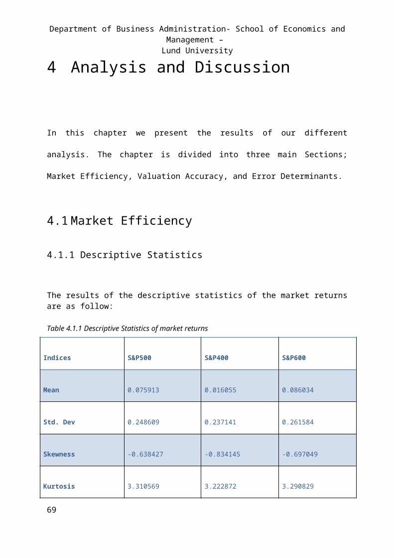
Department of Business Administration- School of Economics and Management – Lund University
Appendix B
69
B1 – B8: Valuation Errors - Descriptive Statistics

Berglund Oscar Zisiadou Argyro

Department of Business Administration- School of Economics and Management – Lund University
71

Berglund Oscar Zisiadou Argyro
B9: Average Valuation Errors - Total Sample

Department of Business Administration- School of Economics and Management – Lund University
B10: Average Valuation Errors - Large Cap.
73

Berglund Oscar Zisiadou Argyro
B11: Average Valuation Errors – Mid Cap.

Department of Business Administration- School of Economics and Management – Lund University
B12: Average Valuation Errors – Small Cap.
75

Berglund Oscar Zisiadou Argyro
B13: P/E Median Error Determinants & Diagnostic Tests
B14: P/E Average Error Determinants & Diagnostic Tests

Department of Business Administration- School of Economics and Management – Lund University
77
B15: P/E Harmonic Error Determinants & Diagnostic Tests
B16: P/S Median Error Determinants & Diagnostic Tests

Berglund Oscar Zisiadou Argyro
B17: P/S Average Error Determinants & Diagnostic Tests
B18: P/S Harmonic Error Determinants & Diagnostic Tests

Department of Business Administration- School of Economics and Management – Lund University
79
B19: P/EBITDA Median Error Determinants & Diagnostic Tests
B20: P/EBITDA Average Error Determinants & Diagnostic Tests

Berglund Oscar Zisiadou Argyro
B21: P/EBITDA Harmonic Error Determinants & Diagnostic Tests
B22: P/EBIT Median Error Determinants & Diagnostic Tests
B23: P/EBIT Average Error Determinants & Diagnostic Tests
B24: P/EBIT Harmonic Error Determinants & Diagnostic Tests
B25: P/(EBIT+RD) Median Error Determinants & Diagnostic Tests
B27: P/(EBIT+RD) Harmonic Error Determinants & Diagnostic Tests
B29: P/TA Average Error Determinants & Diagnostic Tests

Department of Business Administration- School of Economics and Management – Lund University
81
B31: EV/EBITDA Median Error Determinants & Diagnostic Tests
B32: EV/EBITDA Average Error Determinants & Diagnostic Tests
B33: EV/EBITDA Harmonic Error Determinants & Diagnostic Tests
B34: PEV/EBIT Median Error Determinants & Diagnostic Tests
B35: EV/EBIT Average Error Determinants & Diagnostic Tests
B36: EV/EBIT Harmonic Error Determinants & Diagnostic Tests
B37: P/e (1) Median Error Determinants & Diagnostic Tests

Berglund Oscar Zisiadou Argyro
B39: P/E (1) Harmonic Error Determinants & Diagnostic Tests
B40: P/EBITDA (1) Median Error Determinants & Diagnostic Tests
B41 : P/EBITDA (1) Average Error Determinants & Diagnostic Tests
B42: P/EBITDA (1) Harmonic Error Determinants & Diagnostic Tests
B43: EV/EBITDA (1) Median Error Determinants & Diagnostic Tests

Department of Business Administration- School of Economics and Management – Lund University
83
B45 : EV/EBITDA (1) Harmonic Error Determinants & Diagnostic Tests

Berglund Oscar Zisiadou Argyro
Appendix C
C1: Variable Codes
Variable Code Variable Code
Assets WC02999 Market/Book PTBV
Volatility WC08806 R&D WC01201
Enterprise Value WC18100 EBIT WC18191
EBITDA WC18198 Sales DWSL
Earnings WC07250 Stock Price P
P/S FTSPS Profit Margin WC08316
S&P400 S&PMID P/E PE
10-year gov index U.S BMUS10Y Capitalization MV
12-month forward Enterprise Value DIEV S&P500 $SPX
12-month forward P/E PEFD12 S&P600 S&P600I
12-month forward EBITDA EBD1FD12 10-year treas. bond U.S S00311
C2: List of Multiples
List of MultiplesP/EP/E (1)P/SP/EBITP/(EBIT+RD)P/EBITDAP/EBITDA (1)P/TAEV/EBITEV/EBITDAEV/EBITDA (1)