1 Global Emissions of Air Pollutants and Greenhouse Gases John van Aardenne Climate Change Unit...
51
1 Global Emissions of Air Pollutants and Greenhouse Gases John van Aardenne Climate Change Unit Acknowledgements: Valerio Pagliari (Italy), Suvi Monni (Finland), Jos Olivier (Netherlands), Jeroen Peters (Netherlands), Lorenzo Orlandini (Italy),Fulgencio SanMartin (Spain), Ulrike Doering (Germany).
-
Upload
merilyn-carson -
Category
Documents
-
view
216 -
download
3
Transcript of 1 Global Emissions of Air Pollutants and Greenhouse Gases John van Aardenne Climate Change Unit...
1
Global Emissions of Air Pollutants and Greenhouse Gases
John van AardenneClimate Change Unit
Acknowledgements: Valerio Pagliari (Italy), Suvi Monni (Finland), Jos Olivier (Netherlands), Jeroen Peters (Netherlands), Lorenzo Orlandini (Italy),Fulgencio SanMartin (Spain), Ulrike Doering (Germany).

2
Overview of presentation
Overview
1. Introduction: Global emission Inventory research at European Commission
2. Task Force on Hemispheric Transport of Air Pollution
3. Large scale emissions inventories: calculation of emissions for ~240 countries
4. Overview of existing knowledge
5. Special case: emissions from international marine transport
Discussion- Can insights from global emission inventories help you in compiling your emission
inventory?
- Your inventory will provide us with insights on the “local” situation (validation)
3
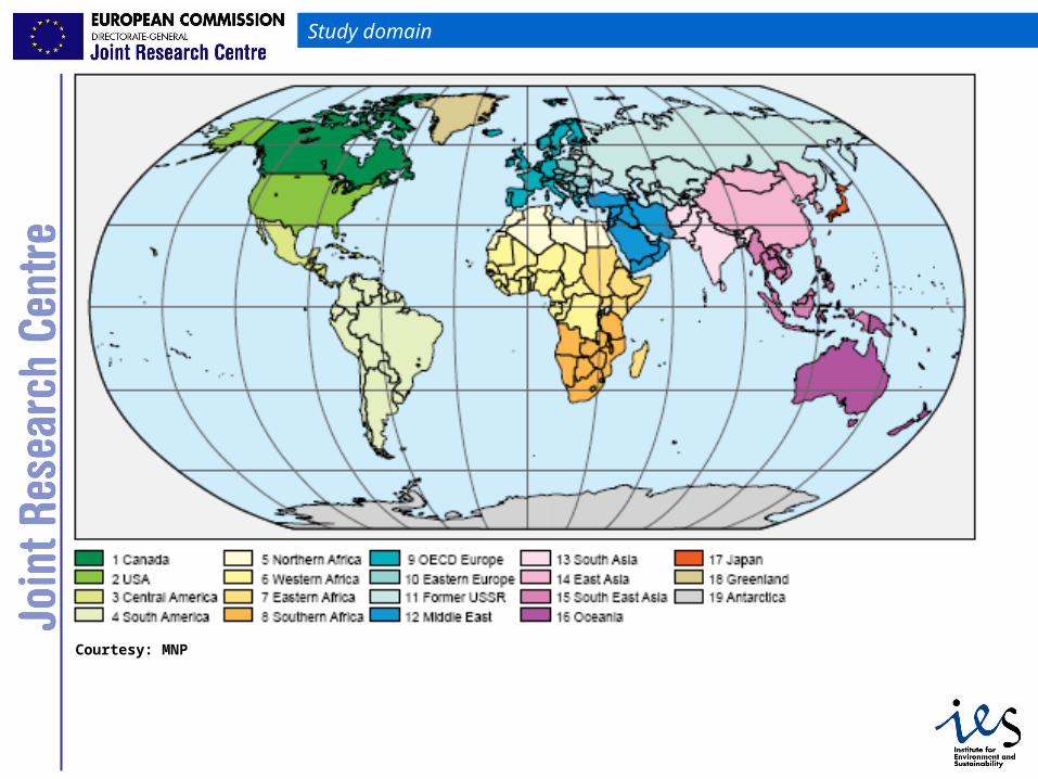
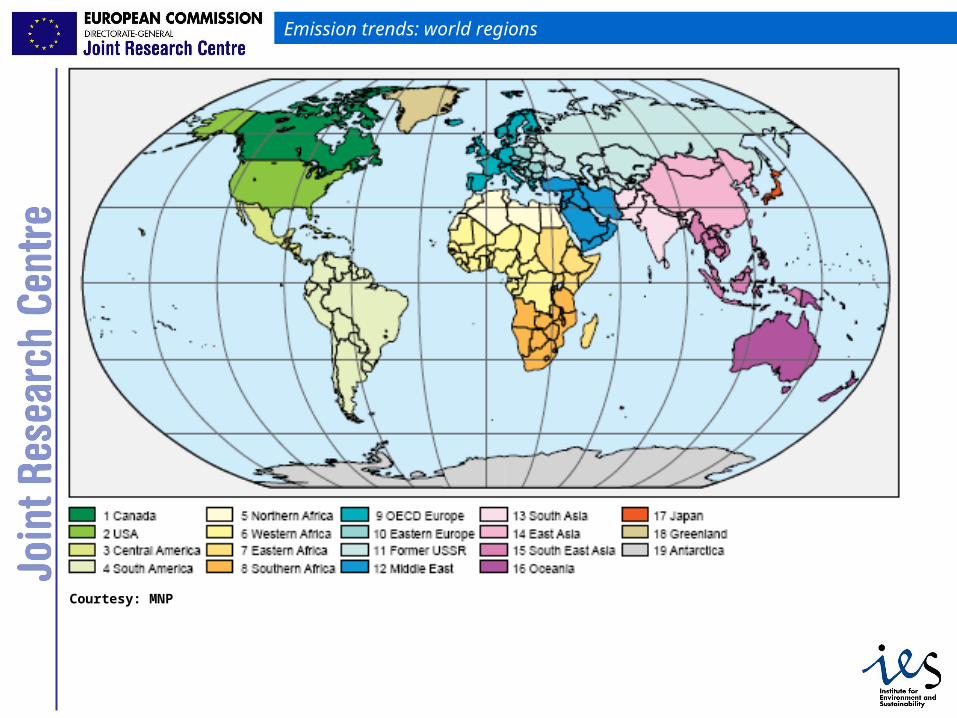
Study domain
Courtesy: MNP

4
1. Climate change unit
Global Air Pollution and Climate
Integrated ClimatePolicy Assessment
Unit head: Frank Raes~ 45 staff members
Greenhouse Gases - Agriculture, Forestry and other Land Uses
Frank Dentener
Guenther Seufert
John van Aardenne

5
Different uses of emission inventories
Inventories for policy purposes: - monitoring the progress/compliance in meeting specific emission targets
(National, Kyoto, LRTAP)- deciding which activities should be regulated to reduce emissions
Inventories for scientific purposes:- understanding the processes that lead to anthropogenic and natural
emissions- understanding past, present and future change in atmospheric composition
due to emissions (through atmospheric dispersion modeling)
Science for policy:- impact modeling (inventories used to calculate impact on health,
ecosystems)- assessment of transport of air pollutants across country borders and
continents (e.g. HTAP modeling).
6
CLRTAPTask Force on Hemispheric Transport of Air Poluttion

7
HTAP
Task Force on Hemispheric Transport of Air Pollution
- Parties of the Convention on Long-range Transboundary Air Pollution (CLRTAP) decided to create a new task force to develop a fuller understanding of the intercontinental transport of air pollutants in the Northern Hemisphere and to produce estimates of the intercontinental flows of air pollutants for consideration in the review of protocols under the Convention.
8
HTAP and emission inventories
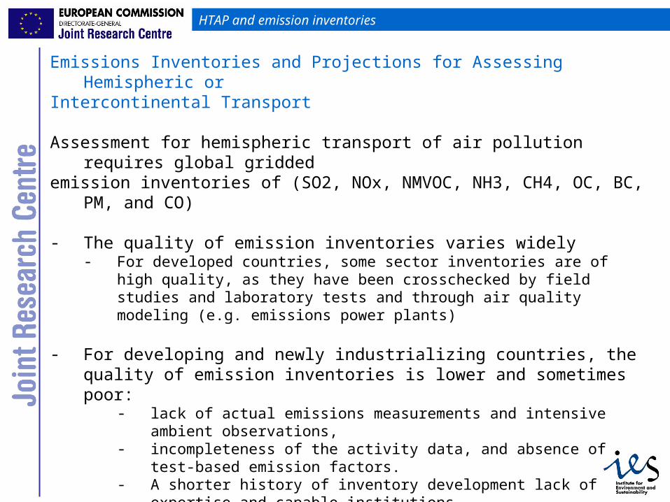
Emissions Inventories and Projections for Assessing Hemispheric or Intercontinental Transport
Assessment for hemispheric transport of air pollution requires global griddedemission inventories of (SO2, NOx, NMVOC, NH3, CH4, OC, BC, PM, and CO)
- The quality of emission inventories varies widely- For developed countries, some sector inventories are of high quality, as they
have been crosschecked by field studies and laboratory tests and through air quality modeling (e.g. emissions power plants)
- For developing and newly industrializing countries, the quality of emission inventories is lower and sometimes poor:
- lack of actual emissions measurements and intensive ambient observations,
- incompleteness of the activity data, and absence of test-based emission factors.
- A shorter history of inventory development lack of expertise and capable institutions.
9
HTAP and emission inventories
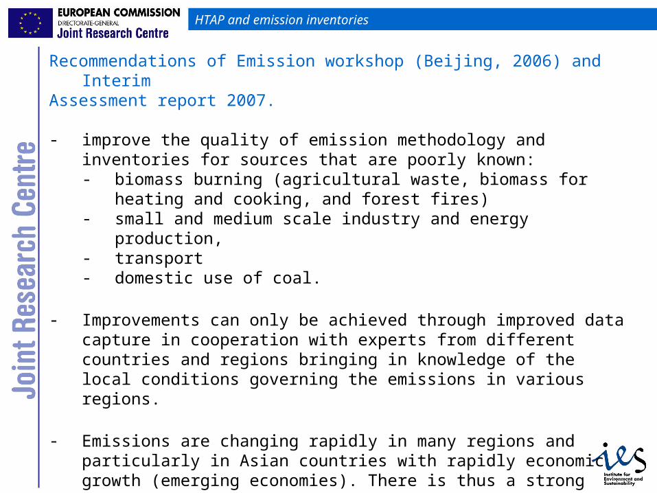
Recommendations of Emission workshop (Beijing, 2006) and Interim Assessment report 2007.
- improve the quality of emission methodology and inventories for sources that are poorly known:- biomass burning (agricultural waste, biomass for heating and cooking,
and forest fires) - small and medium scale industry and energy production, - transport- domestic use of coal.
- Improvements can only be achieved through improved data capture in cooperation with experts from different countries and regions bringing in knowledge of the local conditions governing the emissions in various regions.
- Emissions are changing rapidly in many regions and particularly in Asian countries with rapidly economic growth (emerging economies). There is thus a strong need to update any emission data base to hold as recent data as possible.
10
GEIA/ACCENT Workshop on non-OECD emission inventories (Feb 2006)
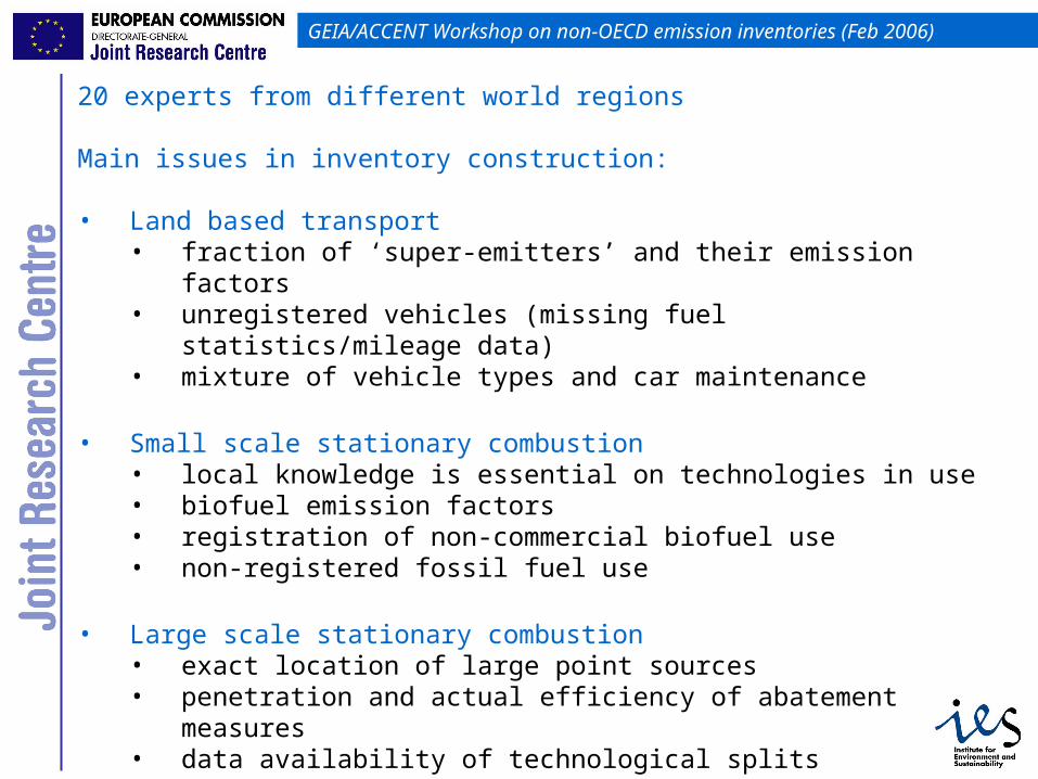
20 experts from different world regions
Main issues in inventory construction:
• Land based transport• fraction of ‘super-emitters’ and their emission factors• unregistered vehicles (missing fuel statistics/mileage data)• mixture of vehicle types and car maintenance
• Small scale stationary combustion• local knowledge is essential on technologies in use • biofuel emission factors• registration of non-commercial biofuel use• non-registered fossil fuel use
• Large scale stationary combustion• exact location of large point sources • penetration and actual efficiency of abatement measures• data availability of technological splits• activities in Industrial processes

11
Large scale emission inventories

12
Methodological aspects: overview
Simplified equation of emission factor approach
EMISSION = AD x EF (1-(IC x RE))
AD = activity data by sector and technologyEF = uncontrolled emission factor by sector, technology, compoundIC = installed capacity of abatement measure by sector, technologyRE = removal efficiency of abatement measure, by compound
13
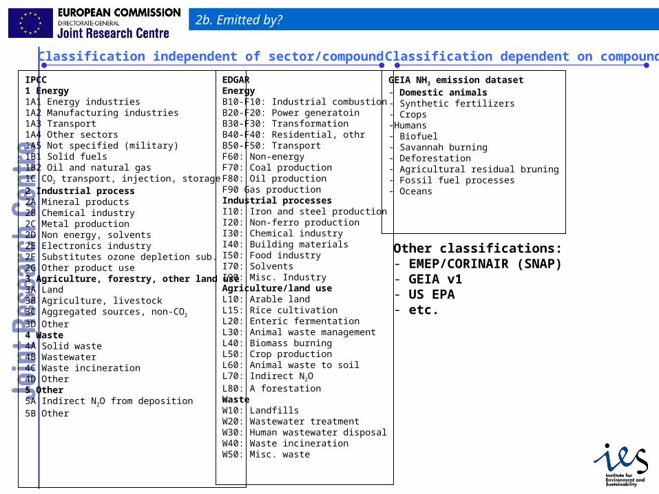
2b. Emitted by?
IPCC1 Energy1A1 Energy industries1A2 Manufacturing industries1A3 Transport1A4 Other sectors1A5 Not specified (military)1B1 Solid fuels1B2 Oil and natural gas1C CO2 transport, injection, storage2 Industrial process2A Mineral products2B Chemical industry2C Metal production2D Non energy, solvents2E Electronics industry2F Substitutes ozone depletion sub.2G Other product use3 Agriculture, forestry, other land use3A Land3B Agriculture, livestock3C Aggregated sources, non-CO2
3D Other4 Waste4A Solid waste4B Wastewater4C Waste incineration4D Other5 Other5A Indirect N2O from deposition5B Other
EDGAREnergyB10-F10: Industrial combustionB20-F20: Power generatoinB30-F30: TransformationB40-F40: Residential, othrB50-F50: TransportF60: Non-energyF70: Coal productionF80: Oil productionF90 Gas productionIndustrial processesI10: Iron and steel productionI20: Non-ferro productionI30: Chemical industryI40: Building materialsI50: Food industryI70: SolventsI90: Misc. IndustryAgriculture/land useL10: Arable landL15: Rice cultivationL20: Enteric fermentationL30: Animal waste managementL40: Biomass burningL50: Crop productionL60: Animal waste to soilL70: Indirect N2OL80: A forestationWasteW10: LandfillsW20: Wastewater treatmentW30: Human wastewater disposalW40: Waste incinerationW50: Misc. waste
Other classifications:- EMEP/CORINAIR (SNAP)- GEIA v1- US EPA- etc.
GEIA NH3 emission dataset- Domestic animals- Synthetic fertilizers- Crops-Humans- Biofuel- Savannah burning- Deforestation- Agricultural residual bruning- Fossil fuel processes- Oceans
Classification independent of sector/compound Classification dependent on compound
14
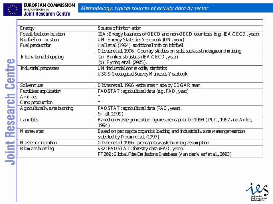
Methodology: typical sources of activity data by sector
Energy Source of information Fossil fuel combustion Biofuel combustion Fuel production
IEA: Energy balances of OECD and non-OECD countries (e.g. IEA/OECD, year). UN: Energy Statistics Yearbook (UN, year) Hall et al (1994) additional info on biofuel Olivier et al. 1996: Country studies on split surface/underground mining
International shipping (a) Bunker statistics (IEA/OECD, year) (b) Eyring et al. (2005).
Industrial processes
UN industrial commodity statistics USGS Geological Survey Minerals Yearbook
Solvent use Olivier et al. 1996: estimates made by EDGAR team Fertilizer application Animals Crop production
FAOSTAT: agricultural data (e.g. FAO, year) “ “
Agricultural waste burning FAOSTAT: agricultural data (FAO, year). Smill (1999)
Landfills
Based on waste generation figures per capita for 1990 (IPCC, 1997 and Adler, 1994)
Wastewater
Based on per capita organics loading and industrial waste water generation selected by Doorn et al. (1997)
Waste incineration Olivier et al. 1996: per capita waste burning assumption Biomass burning
v32: FAOSTAT: forestry data (FAO, year). FT200: Global Fire Emissions Database (Van der Werf et al., 2003)

15
Activity data
AD: Fuel combusted in public power plants (ktoe) in The Netherlands (IEA, 2006)
0
2000
4000
6000
8000
10000
12000
14000
16000
18000
20000
2000 2001 2002 2003 2004
Residual Fuel Oil
Gas/Diesel Oil
Refinery Gas
Natural Gas
Biogas
Primary Solid Biomass
Blast Furnace Gas
Coke Oven Gas
Other Bituminous Coal
16
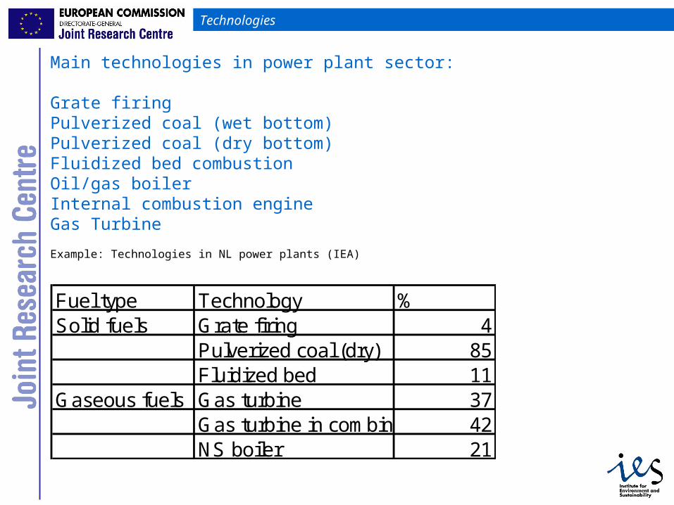
Technologies
Main technologies in power plant sector:
Grate firingPulverized coal (wet bottom)Pulverized coal (dry bottom)Fluidized bed combustionOil/gas boilerInternal combustion engineGas Turbine
Example: Technologies in NL power plants (IEA)
Fuel type Technology %Solid fuels Grate firing 4
Pulverized coal (dry) 85Fluidized bed 11
Gaseous fuels Gas turbine 37Gas turbine in combined cycle 42NS boiler 21
17
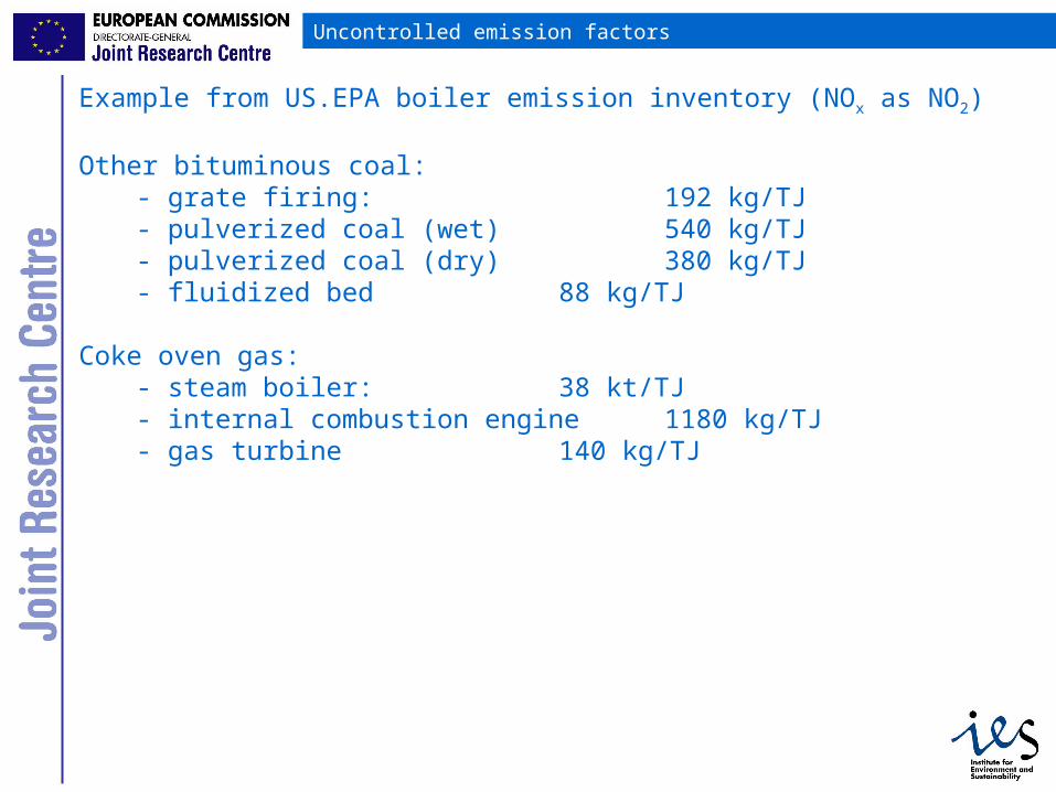
Uncontrolled emission factors
Example from US.EPA boiler emission inventory (NOx as NO2)
Other bituminous coal: - grate firing: 192 kg/TJ- pulverized coal (wet) 540 kg/TJ- pulverized coal (dry) 380 kg/TJ- fluidized bed 88 kg/TJ
Coke oven gas:- steam boiler: 38 kt/TJ- internal combustion engine 1180 kg/TJ- gas turbine 140 kg/TJ
18
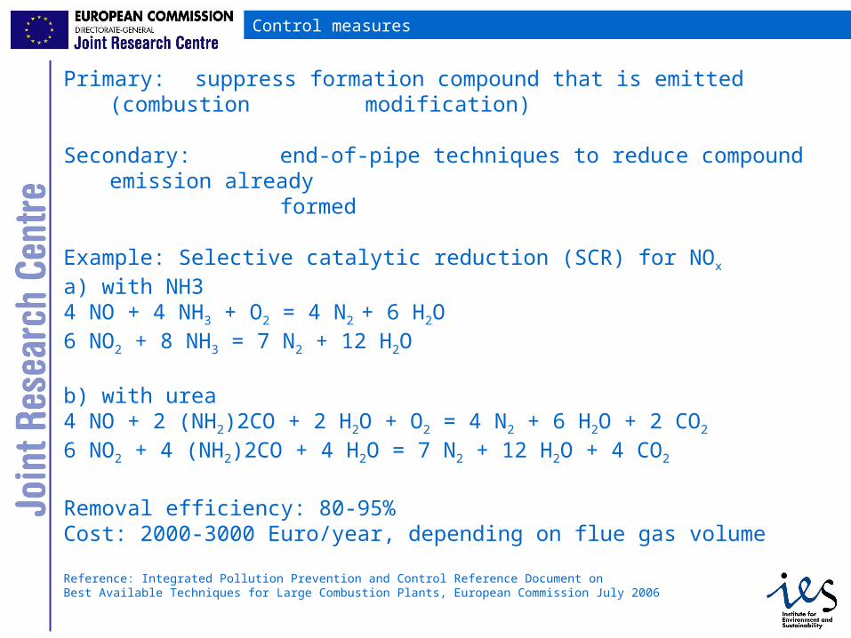
Control measures
Primary: suppress formation compound that is emitted (combustion modification)
Secondary: end-of-pipe techniques to reduce compound emission alreadyformed
Example: Selective catalytic reduction (SCR) for NOx
a) with NH34 NO + 4 NH3 + O2 = 4 N2 + 6 H2O6 NO2 + 8 NH3 = 7 N2 + 12 H2O
b) with urea 4 NO + 2 (NH2)2CO + 2 H2O + O2 = 4 N2 + 6 H2O + 2 CO2
6 NO2 + 4 (NH2)2CO + 4 H2O = 7 N2 + 12 H2O + 4 CO2
Removal efficiency: 80-95%Cost: 2000-3000 Euro/year, depending on flue gas volume
Reference: Integrated Pollution Prevention and Control Reference Document onBest Available Techniques for Large Combustion Plants, European Commission July 2006

19
Selection of emissions data as typically found in literature
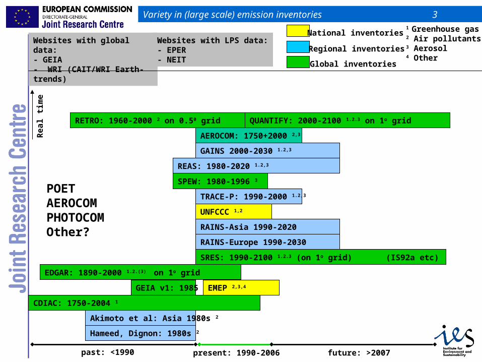
20past: <1990 present: 1990-2006 future: >2007
UNFCCC 1,2
EMEP 2,3,4
National inventories
Global inventories
Regional inventories
EDGAR: 1890-2000 1.2.(3) on 1o grid
RETRO: 1960-2000 2 on 0.50 grid
1 Greenhouse gas2 Air pollutants3 Aerosol4 Other
QUANTIFY: 2000-2100 1.2.3 on 1o grid
GEIA v1: 1985
CDIAC: 1750-2004 1
SRES: 1990-2100 1.2.3 (on 1o grid) (IS92a etc)
SPEW: 1980-1996 3
RAINS-Europe 1990-2030
RAINS-Asia 1990-2020
GAINS 2000-2030 1.2,3
Websites with global data:- GEIA- WRI (CAIT/WRI Earth-trends)
Websites with LPS data:- EPER- NEIT
Akimoto et al: Asia 1980s 2
Hameed, Dignon: 1980s 2
REAS: 1980-2020 1.2,3
TRACE-P: 1990-2000 1.2,3POETAEROCOMPHOTOCOMOther?
Variety in (large scale) emission inventories 3
AEROCOM: 1750+2000 2,3Re
al
tim
e
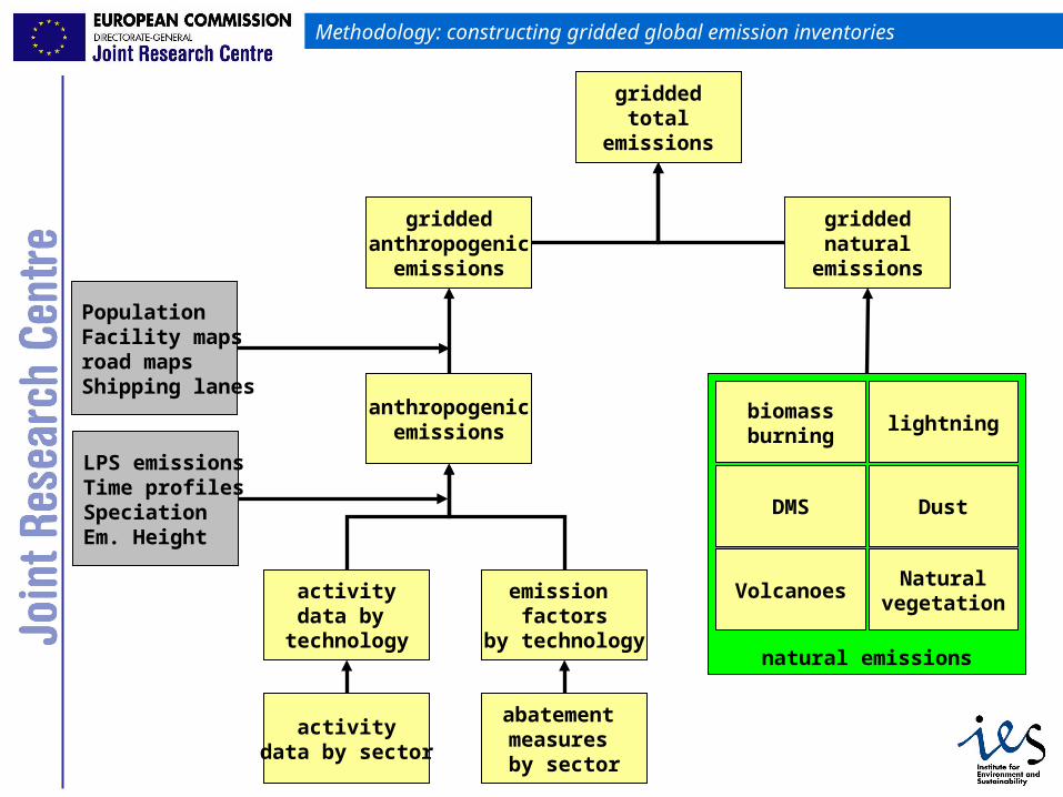
21
Methodology: constructing gridded global emission inventories
activitydata by sector
activitydata by
technology
emission factors
by technology
abatement measures by sector
anthropogenicemissions
griddedanthropogenic
emissions
PopulationFacility mapsroad mapsShipping lanes
LPS emissionsTime profilesSpeciationEm. Height
griddedtotal
emissions
griddednatural
emissions
natural emissions
biomassburning
lightning
DMS Dust
VolcanoesNatural
vegetation

22
2c. Importance of different sector
The relative importance for global emissions of different sectors and fuel types is presented in Table 4.2. The contributions shown in this table can be markedly different, however, for individual countries and regions. The estimates are based on EDGAR FT2000 (Olivier et al., 2005), Bond et al. (2004), EDGARv2 (Olivier et al., 1996), and Bouwman et al. (1997).
Species
Large stationary combustion
Small stationary combustion
TransportIndustrial processes
Agriculture WasteBiomass BurningFossil
fuelBiofue
lFossil fuel
Biofuel
Road
Non-road
CO 2 1 3 24 19 1 4 0 0 46
NH3 0 0 0 3 0 0 1 82 6 8
NOx 28 1 2 5 22 13 5 0 0 23
NMVOC 23a 2 1 16 20 3 16 0 2 17
SO2 62 0 5 2 2 6 19 0 0 2
BC 3 2 15 22 14 5 0 0 0 38
OC 1 3 2 21 4 0 0 0 0 69
CH4 30 0 1 4 0 0 0 40 18 6
CO: ~ 900 Tg
NOx: ~ 130 Tg
NMVOC: ~ 165 Tg
SO2: ~150 Tg
BC: ~ 8 Tg
OC: ~33 Tg
CH4: ~320 Tg
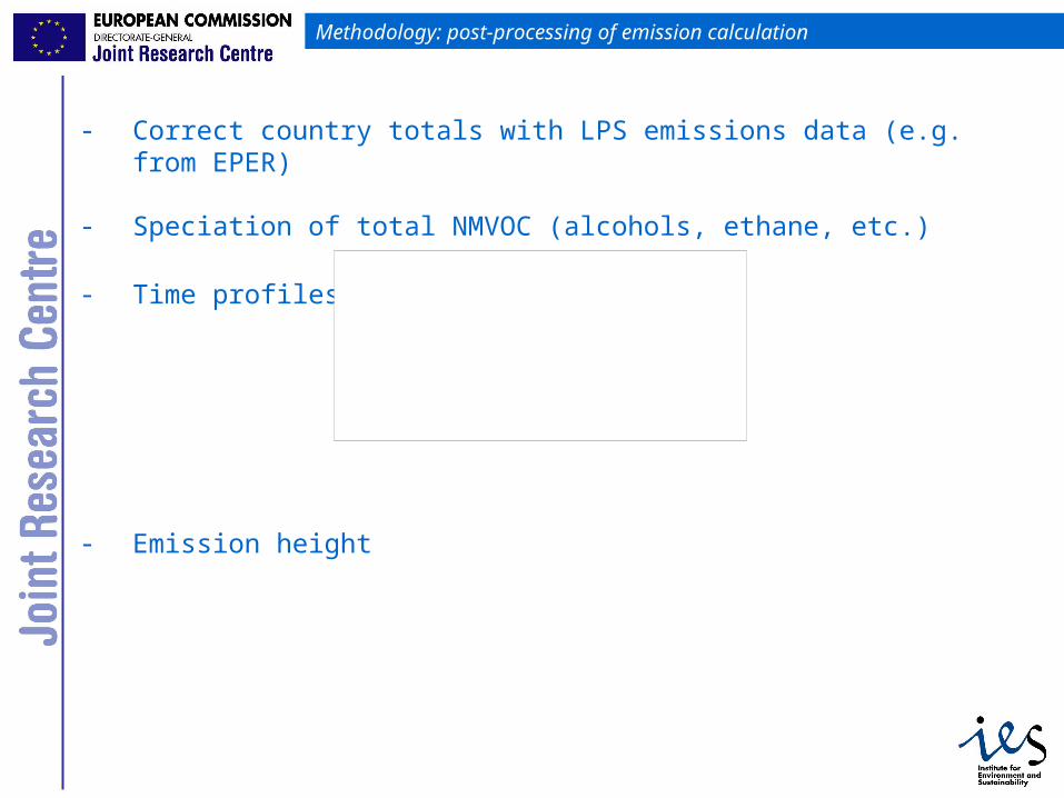
23
Methodology: post-processing of emission calculation
- Correct country totals with LPS emissions data (e.g. from EPER)
- Speciation of total NMVOC (alcohols, ethane, etc.)
- Time profiles
- Emission height
0
0.5
1
1.5
2
2.5
J an Feb Mar Apr May J un J ul Aug Sep Oct Nov Dec
power
industry
residential
refineries
processes
solvent use
traffic
agriculture
LOTOS time profiles, Veldt (1992)

24
Allocation of emissions on grid (1x1 vs 0.1x0.1 grid)

25
Allocation of emissions on grid (1x1 vs. 0.1x0.1 grid)

26
Allocation of emissions on grid (0.1x0.1 grid)
27
Resulting data distributed to modelers
0.0002
0.0005
0.001
0.002
0.005
0.01
0.02
0.05
0.1
0.2
0.5
1
2
5
10
50
0.0002
0.0005
0.001
0.002
0.005
0.01
0.02
0.05
0.1
0.2
0.5
1
2
5
10
50
0.0002
0.0005
0.001
0.002
0.005
0.01
0.02
0.05
0.1
0.2
0.5
1
2
5
10
50
0.0002
0.0005
0.001
0.002
0.005
0.01
0.02
0.05
0.1
0.2
0.5
1
2
5
10
50
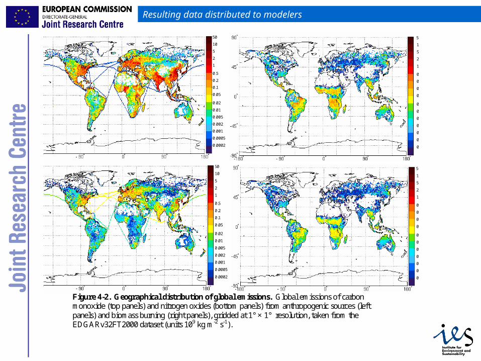
Figure 4-2. Geographical distribution of global emissions. Global emissions of carbon monoxide (top panels) and nitrogen oxides (bottom panels) from anthropogenic sources (left panels) and biomass burning (right panels), gridded at 1° × 1° resolution, taken from the EDGARv32FT2000 dataset (units 109 kg m-2 s-1).

28
Overview of regional emissions
29
Emission trends: world regions
Courtesy: MNP

30
NOx emissions in 2000 (excluding international shipping and aviation)
0% 20% 40% 60% 80% 100%
Canada
USA
Central America
South America
Northern Africa
Western Africa
Eastern Africa
Southern Africa
OECD Europe
Eastern Europe
Former USSR
Middle East
South Asia
East Asia
SE Asia
Oceania
Japan
Large stationary FFC Large stationary BFC Small stationary FFCSmall stationary BFC Transport Industrial processAgricult. waste burning Waste

31
NOx emissions Tg NO2 (including biomass burning, excl shipping/aviation)
Shipping: 9.6 TgAviation: 2.3 Tg
0 2 4 6 8 10 12 14 16 18
Canada
USA
Central America
South America
Northern Africa
Western Africa
Eastern Africa
Southern Africa
OECD Europe
Eastern Europe
Former USSR
Middle East
South Asia
East Asia
SE Asia
Oceania
Japan
Anthropogenic
Biomass burning
32
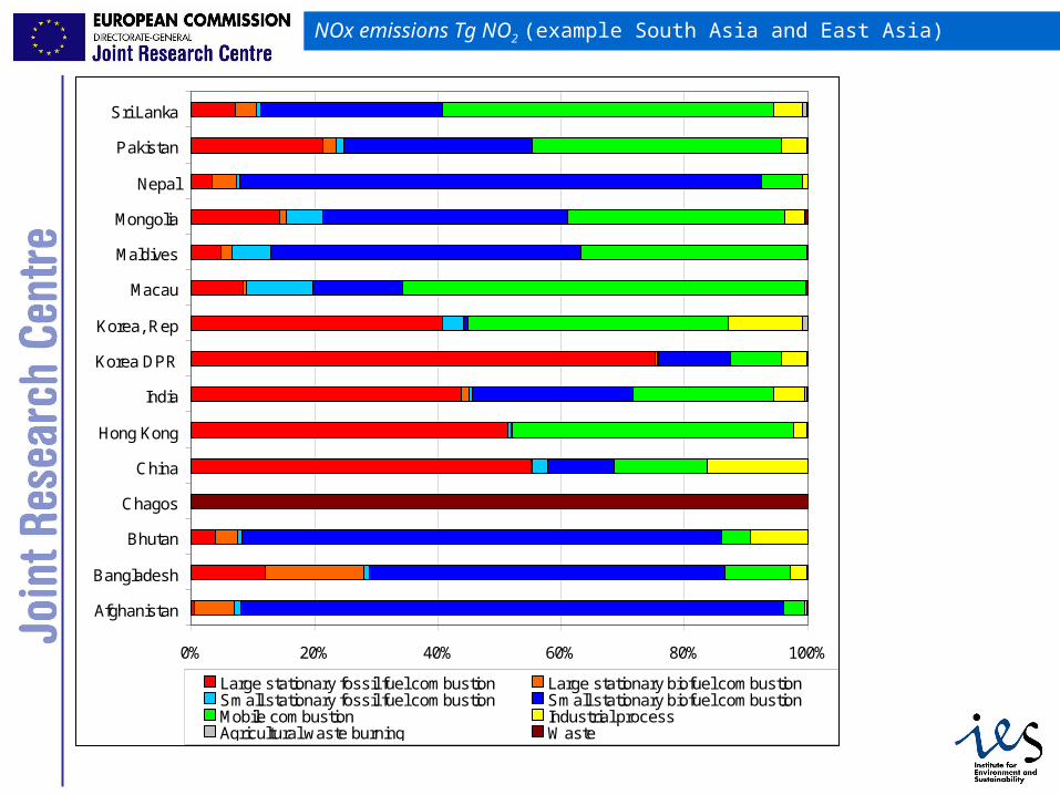
NOx emissions Tg NO2 (example South Asia and East Asia)
0% 20% 40% 60% 80% 100%
Afghanistan
Bangladesh
Bhutan
Chagos
China
Hong Kong
India
Korea DPR
Korea, Rep
Macau
Maldives
Mongolia
Nepal
Pakistan
Sri Lanka
Large stationary fossil fuel combustion Large stationary biofuel combustionSmall stationary fossil fuel combustion Small stationary biofuel combustionMobile combustion Industrial processAgricultural waste burning Waste

33
NOx Contribution of road transport to grid cell emission
Butler, Lawrence, Gurjar, van Aardenne, Schultz and Lelieveld, the representation ofmegacities in global emission inventories, submitted to Atmospheric Environment, 2007

34
CO emissions in 2000 (excluding international shipping and aviation)
0% 20% 40% 60% 80% 100%
Canada
USA
Central America
South America
Northern Africa
Western Africa
Eastern Africa
Southern Africa
OECD Europe
Eastern Europe
Former USSR
Middle East
South Asia
East Asia
SE Asia
Oceania
Japan
Large stationary fossil fuel combustion Large stationary biofuel combustionSmall stationary fossil fuel combustion Small stationary biofuel combustionMobile combustion Industrial processAgricultural waste burning Waste

35
CO emissions Tg CO (including biomass burning, excl shipping/aviation)
Shipping: 0.1 TgAviation: 1.8 Tg
0 20 40 60 80 100 120 140 160
Canada
USA
Central America
South America
Northern Africa
Western Africa
Eastern Africa
Southern Africa
OECD Europe
Eastern Europe
Former USSR
Middle East
South Asia
East Asia
SE Asia
Oceania
Japan
Anthropogenic
Biomass burning
36
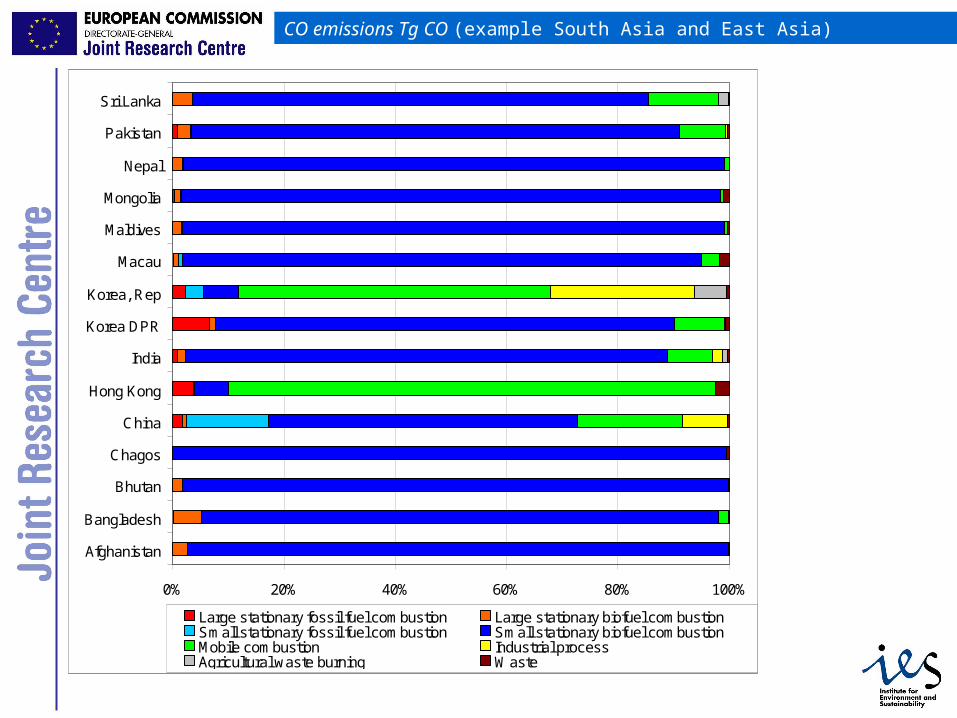
CO emissions Tg CO (example South Asia and East Asia)
0% 20% 40% 60% 80% 100%
Afghanistan
Bangladesh
Bhutan
Chagos
China
Hong Kong
India
Korea DPR
Korea, Rep
Macau
Maldives
Mongolia
Nepal
Pakistan
Sri Lanka
Large stationary fossil fuel combustion Large stationary biofuel combustionSmall stationary fossil fuel combustion Small stationary biofuel combustionMobile combustion Industrial processAgricultural waste burning Waste

37
CO: Contribution of residential biofuel combustion to grid cell emission
Butler, Lawrence, Gurjar, van Aardenne, Schultz and Lelieveld, the representation ofmegacities in global emission inventories, in preparation.

38
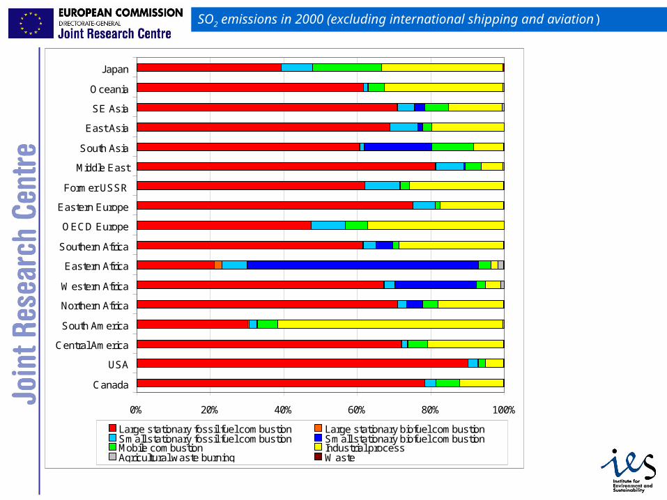
SO2 emissions in 2000 (excluding international shipping and aviation)
0% 20% 40% 60% 80% 100%
Canada
USA
Central America
South America
Northern Africa
Western Africa
Eastern Africa
Southern Africa
OECD Europe
Eastern Europe
Former USSR
Middle East
South Asia
East Asia
SE Asia
Oceania
Japan
Large stationary fossil fuel combustion Large stationary biofuel combustionSmall stationary fossil fuel combustion Small stationary biofuel combustionMobile combustion Industrial processAgricultural waste burning Waste

39
SO2 emissions Tg SO2 (including biomass burning, excl shipping/aviation)
Shipping: 7.3 TgAviation: 0.2 Tg
0 5 10 15 20 25 30 35 40 45
Canada
USA
Central America
South America
Northern Africa
Western Africa
Eastern Africa
Southern Africa
OECD Europe
Eastern Europe
Former USSR
Middle East
South Asia
East Asia
SE Asia
Oceania
Japan
Anthropogenic
Biomass burning
40
SO2 emissions in 2000 (excluding international shipping and aviation)
0% 20% 40% 60% 80% 100%
Canada
USA
Central America
South America
Northern Africa
Western Africa
Eastern Africa
Southern Africa
OECD Europe
Eastern Europe
Former USSR
Middle East
South Asia
East Asia
SE Asia
Oceania
Japan
Large stationary fossil fuel combustion Large stationary biofuel combustionSmall stationary fossil fuel combustion Small stationary biofuel combustionMobile combustion Industrial processAgricultural waste burning Waste
41
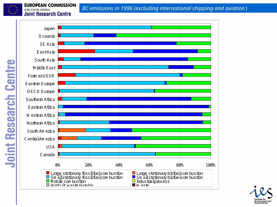
BC emissions in 1996 (excluding international shipping and aviation)
0% 20% 40% 60% 80% 100%
Canada
USA
Central America
South America
Northern Africa
Western Africa
Eastern Africa
Southern Africa
OECD Europe
Eastern Europe
Former USSR
Middle East
South Asia
East Asia
SE Asia
Oceania
Japan
Large stationary fossil fuel combustion Large stationary biofuel combustionSmall stationary fossil fuel combustion Small stationary biofuel combustionMobile combustion Industrial processAgricult. waste burning Waste

42
OC emissions in 1996 (excluding international shipping and aviation)
0% 20% 40% 60% 80% 100%
Canada
USA
Central America
South America
Northern Africa
Western Africa
Eastern Africa
Southern Africa
OECD Europe
Eastern Europe
Former USSR
Middle East
South Asia
East Asia
SE Asia
Oceania
Japan
Large stationary fossil fuel combustion Large stationary biofuel combustionSmall stationary fossil fuel combustion Small stationary biofuel combustionMobile combustion Industrial processAgricult. waste burning Waste

43
Emissions from selected countries fromEDGAR calculations
(CO, NMVOC, NOx, SO2 1990, 1995, 2000)

44
“your emissions are wrong !”
YES, WE KNOW !

45
General problems in emission inventory calculations
(i) Not practical possible to monitor each individual emission source:Emission factor approach is adopted: Emission = activity x emission factor
(ii) We know that emission inventories are inaccurate representations of emission that has actually occurred:
i
N
iinventoryreal EE
1
Examples of errors i:
aggregation error Calculation of emissions on other spatial, temporal scale and for emissions sources that are different from scale on which emissions occur in reality
extrapolation error
Due to lack of measurements of emission rates or activity data, non-specific data are extrapolated
Measurement error
Errors in measurement lead to inaccurate values of emission factors of activity data
(iii) Often, we do not know the extent to which emission inventories are inaccurate
- detailed review of existing inventories not performed yet- several inventories are non-transparent about method and data- lack of different independent inventories- lack of measurement data and model studies to confront inventories with
46
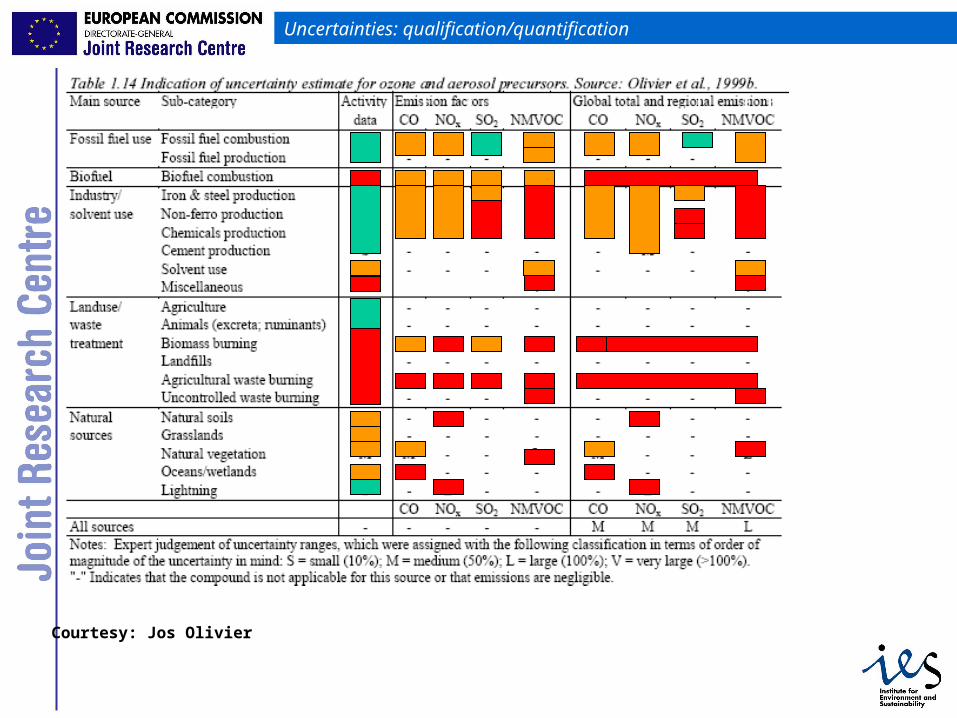
Uncertainties: qualification/quantification
Courtesy: Jos Olivier
47
0
10
20
30
40
50
60
70
80
1990 1991 1992 1993 1994 1995 1996 1997 1998 1999 2000
year
Gg
CO
, NO
2
0.90
0.95
1.00
1.05
1.10
1.15
1.20
frac
tio
n c
om
par
ed t
o 1
990
NOx_India (2nd axis) CO_India (2nd axis) NOx_Delhi CO_Delhi
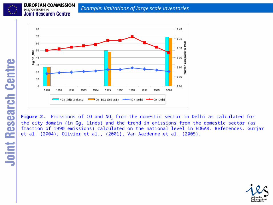
Figure 2. Emissions of CO and NO2 from the domestic sector in Delhi as calculated for the city domain (in Gg, lines) and the trend
in emissions from the domestic sector (as fraction of 1990 emissions) calculated on the national level in EDGAR. References. Gurjar et al. (2004); Olivier et al., (2001), Van Aardenne et al. (2005).
Example: limitations of large scale inventories
48
Example: emissions from international shipping

49
Mobile sources: international shipping (1)
iNOxi iNOx
iiMCRi ii ityr
EIFCTE
SFOCFPFCFCptionFuelconsum
,
132
1
,
132
1
132
11
n Number of sub-groups = 132
Pi Accumulated installed engine power for each subgroup
FMCR,i Engine load factor based on duty cycle profile
i[hrs/yr] Average engine running hours for each sub-group
SFOCg/kWhPower-based specific fuel oil consumption
EIg/kWh Power-based emission factor for each pollutant (NOx, SOX, CO2, HC, PM)
50
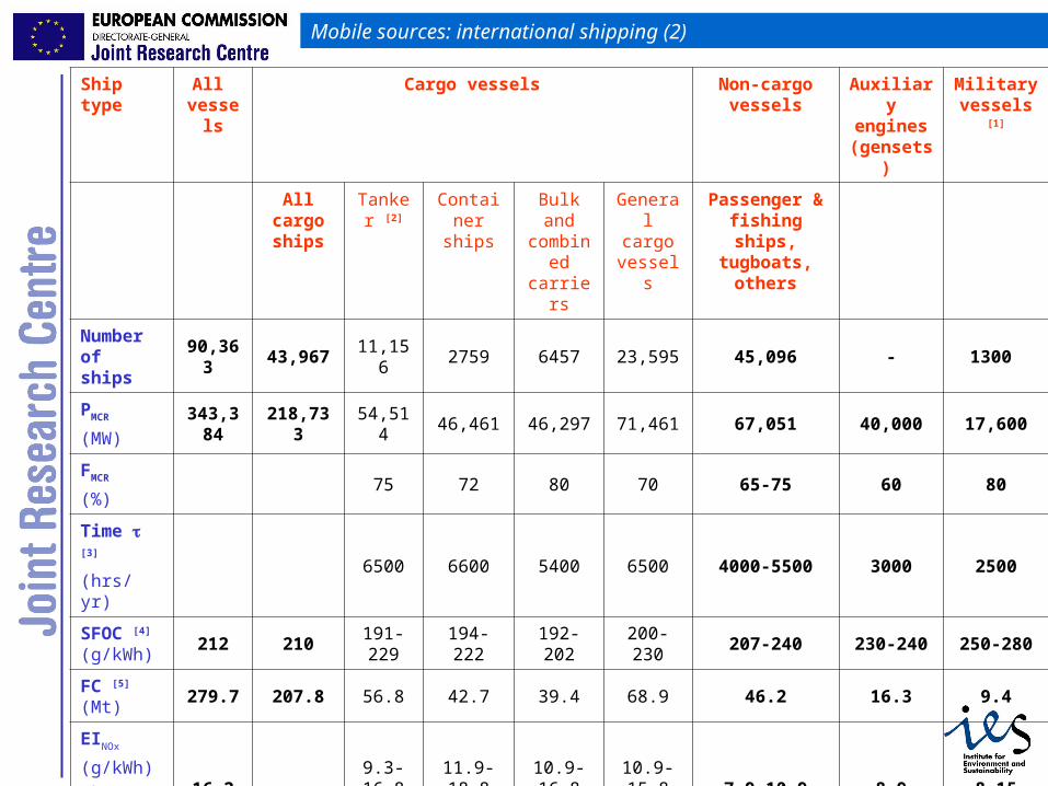
Mobile sources: international shipping (2)
Ship type All vessels
Cargo vessels Non-cargo vessels
Auxiliary engines
(gensets)
Military vessels [1]
All cargo ships
Tanker [2]
Container ships
Bulk and combined carriers
General cargo
vessels
Passenger & fishing ships,
tugboats, others
Number of ships
90,363 43,967 11,156 2759 6457 23,595 45,096 - 1300
PMCR
(MW)343,384 218,733 54,514 46,461 46,297 71,461 67,051 40,000 17,600
FMCR
(%)75 72 80 70 65-75 60 80
Time [3]
(hrs/yr)6500 6600 5400 6500 4000-5500 3000 2500
SFOC [4] (g/kWh)
212 210191-229
194-222 192-202 200-230 207-240 230-240 250-280
FC [5] (Mt)
279.7 207.8 56.8 42.7 39.4 68.9 46.2 16.3 9.4
EINOx
(g/kWh)
(kg/t fuel)
16.2
76.4
-
85.9
9.3-16.8
50-90
11.9-18.8
64-101
10.9-16.8
58-90
10.9-15.8
58-85
7.9-10.9
42-58
8.9
48
8-15
42-80
TENOx
(Mt NO2) 21.38 17.85 4.44 4.67 3.78 4.96 2.39 0.8 0.34

51
Mobile sources: international shipping (3)