1 Glass-Transition Phenomena in Polymer Blends · whether the physics of glass formation can be...

1Glass-Transition Phenomena in Polymer BlendsIoannis M. Kalogeras

University of Athens, Faculty of Physics, Department of Solid State Physics, Zografos 15784,Greece

1.1Introduction

The ever-increasing demand for polymeric materials with designed multi-functional properties has led to a multiplicity of manufacturing approaches andcharacterization studies, seeking proportional as well as synergistic properties ofnovel composites. Fully integrated in this pursuit, blending and copolymerizationhave provided a pair of versatile and cost-effective procedures by which materialswith complex amorphous or partially crystalline structures are fabricated fromcombinations of existing chemicals [1–3]. Through variations in material’s com-position and processing, a subtle adaptation of numerous chemical (corrosionresistance, resistance to chemicals, etc.), thermophysical (e.g., thermal stability,melting point, degree of crystallinity, and crystallization rate), electrical ordielectric (e.g., conductivity and permittivity), and manufacturing or mechanicalproperties (dimensional stability, abrasion resistance, impact strength, fracturetoughness, gas permeability, recyclability, etc.) can be accomplished effortlessly.It is therefore not surprising the fact that related composites have been widelystudied with respect to their microstructure (e.g., length scale of phase homoge-neity in miscible systems, or type of the segregation of phases in multiphasicmaterials) and the evolution of their behavior and complex relaxation dynamicsas the material traverses the glass transformation range [4–7].The reversible transformation of amorphous materials (including amorphous

regions within semicrystalline polymers) from a molten or rubber-like state into astiff and relatively brittle glassy state is denoted as “glass transition” (or “liquid–glasstransition”). Originally, this term was introduced to describe the striking changes inthermodynamic derivative properties (e.g., heat capacity, compressibility, and ther-mal expansivity) that normally accompany the solidification of a viscous liquid,such as a polymer melt, during cooling or even compression. In time course, how-ever, the term “glass transition” acquired a broader meaning and is now frequently

Encyclopedia of Polymer Blends: Volume 3: Structure, First Edition. Edited by Avraam I. Isayev. 2016 Wiley-VCH Verlag GmbH & Co. KGaA. Published 2016 by Wiley-VCH Verlag GmbH & Co. KGaA.

1

employed for describing “any phenomenon that is caused by a timescale (on whichsome interesting degree of freedom equilibrates) becoming longer than the time-scale on which the system is being observed” [6]. The conventional route to theglassy state of matter is the (rapid) cooling of a melt, provided that crystalization isbypassed. Interestingly, melt mixing provides one of the most common techniquesfor the large-scale preparation of compression or injection molded polymer blends.The freezing-in of a structural state during cooling, commonly referred to as glass-ification or vitrification, corresponds to a loss of the state of internal equilibriumpossessed by the initial liquid. The vitrification process occurs over a narrow tem-perature interval, the so-called glass transformation range, over which the charac-teristic molecular relaxation time of the system changes by some 2–2.5 orders ofmagnitude, reaching the order of 100 s (the laboratory timescale). In macro-molecular substances, this relaxation time is connected with the time response ofcooperative (long-range) segmental motions. For convenience, the glass transforma-tion region is traditionally represented by a single value, denoted as the “glass-tran-sition temperature” (Tg) [7]. Because of the range of temperature involved and alsobecause of its history, path, and cooling (or heating) rate dependences, assigning acharacteristic Tg to a system becomes frequently a problematic task. Nonetheless,when appropriately measured, the glass-transition temperature is very reproducibleand has become recognized as one of the most important material properties,directly relating to several other thermophysical and rheological properties, process-ing parameters, and fields of potential application [8].Nowadays, polymer engineering largely relies on chemical and compositional

manipulation of Tg, in an attempt to target particular technological or industrialrequirements. A notable paradigm provides meticulous studies on the physical sta-bilization of active pharmaceutical ingredients (typically, poorly soluble drugs, butpotentially also of proteins or other compounds) in the form of binary or ternarysolid dispersions/solutions with biologically inert glassy polymers, with the aim ofincreasing their solubility, dissolution rate, bioavailability, and therapeutic effective-ness [9]. Significant improvements in the performance of related systems are fre-quently accredited to a combination of factors, including the effects of hydrogen-bonding networks or ion–dipole intercomponent interactions (i.e., stabilizingenthalpic contributions), and strong crystallization-inhibitory steric effects owing tothe high viscosity of the polymeric excipient [10]. The implementation of solid-stateglassy formulations as a means to preserve the native state of proteins (biopreserva-tion) entails a higher level of complexity in behavior, since chemical and physicalstabilization heavily relies on manipulating the local anharmonic motions of theindividual protein molecules (fast dynamics) in addition to their slow (glass-transi-tion) dynamics [11]. The established practice in the preservation of proteins primar-ily focuses on hydrated solid-state mixtures of proteins with glass-formingdisaccharides (e.g., trehalose or sucrose) or polyols (e.g., glycerol), serving as lyopro-tectants. Still, processing problems such as surface denaturation, mixture separation,and pH changes that lead to physical and chemical degradations, in addition todegradations occurring on storage, make clear that manufacturing of alternativesolid-state formulations remains a challenging issue. In this pursuit, however, one

2 1 Glass-Transition Phenomena in Polymer Blends

has to take into account the complex internal protein dynamics and the fact thatin order to successfully maintain protein’s structural integrity the selected glass-forming polymer will have to sustain a strong and complicated hydrogen-bondingnetwork (around and to the protein) that will effectively couple matrix dynamics tothe internal dynamics of the protein molecules [11]; the adaptability in local struc-tures and chemical environments, offered by polymers’ blending, might provide aviable solution to the problem.While general consensus exists as to the usability of glass transitions in exploring

molecular mobilities, molecular environments, and structural heterogeneities in seg-mental length scales, conflicting arguments still appear regarding the interpretationof fundamental phenomenological aspects of the transition itself. The nature of theglass transition remains one of the most controversial problems in the disciplines ofpolymer physics and materials science, and that in spite of the in-depth experimen-tal and theoretical research conducted hitherto [12–14]. The difficulty in treatingglass transitions even in relatively simple linear-chain amorphous polymers iscaused by the almost undetectable changes in static structure, regardless of thequalitative changes in characteristics and the extremely large change in the time-scale. Given the significance of this subject, this chapter begins with an overview ofimportant aspects of the phenomenology of glass formation. To address the per-plexing behavior encountered when a system passes through its glass transforma-tion range, a number of theoretical models approach this phenomenon usingarguments pointing to a thermodynamic or a purely dynamic transition. Althoughwe have not arrived at a comprehensive theory of supercooled liquids and glasses, itis frequently recognized that the observed glass transitions are not bona fide phasetransitions, but rather a dynamical crossover through which a viscous liquid fallsout of equilibrium and displays solid-like behavior on the experimental timescale.Basic notions and derivations of common theoretical models of the glass transitionare presented in Section 1.2, with particular reference to early free volume and con-figurational entropy approaches, in view of their impact on the development of“predictive” relations for the compositional dependence of the Tg in binary polymersystems. Note that regardless of the multitude of treatments we clearly lack a widelyaccepted model that would allow ab initio calculation of the glass-transition tem-perature. Most theoretical approaches simply allow a prediction of changes in Tg

with – among other variables – applied pressure, degree of polymerization (molarmass) or curing (cross-linking), and composition. Important chemical factors thatinfluence the affinity of the components and the magnitude of Tg in polymerblends, in addition to manufacturing processes or treatments that are typically usedfor manipulating the glass-transition temperature of polymer composites, are brieflyreviewed in Section 1.3.The largely experimentally driven scientific interest on glass transitions in

composite materials is equipped with a collection of experimental methods andmeasuring techniques, with the ability to probe molecular motions at distinctlydifferent length scales [15–17]. Most of them introduce different operationaldefinitions of Tg, and some of them are endorsed as scientific standards. In Sec-tion 1.4, fundamental aspects of important experimental means are presented,

1.1 Introduction 3

with emphasis placed on the relative sensitivity and measuring accuracy of eachtechnique, and the proper identification and evaluation of glass transitions inmulticomponent systems. Typically, the broadness of the glass-transition regionis indicative of structural (nano)heterogeneities, whereas its location can beadjusted by appropriate variations in composition and the ensuing changes inthe degree of interchain interactions or material’s free volume. Given the diver-sity of chemical structures of the polymers used and the wide range of dynamicasymmetries and molecular affinities explored, it is not surprising the wealth ofinformation on polymers’ miscibility and the number of phenomena revealed inrelated studies. Two general cases are distinguished experimentally: single-phaseand phase-separated systems. In the first case, for instance in a pair of misciblepolymers or in random copolymers (i.e., with random alternating blocks alongthe macromolecular chain), a single – although rather broad – glass-transitionregion is recorded by most experimental techniques. The glass-transition behav-ior associated with phase separation, a situation characterizing the vast majorityof engineering polymer blends, their related graft, and block copolymers, as wellas interpenetrating polymer networks, demonstrates an elevated level of com-plexity; multiple transitions, ascribed to pure component phases and regions ofpartial mixing, are common experimental findings. Issues related to miscibilityevaluations of polymer blends, such as the determination of the length scale ofstructural heterogeneity using different experimental approaches, are discussedin Section 1.5. The theoretical foundations and practical examples from the anal-ysis of experimental data for miscible systems are critically reviewed in Section1.6. The applicability ranges of important theoretical, semiempirical, or purelyphenomenological mixing rules used for describing the compositional depen-dence of Tg are explored, with examples demonstrating the physical meaning oftheir parameters. A number of case studies, involving intermolecularly hydro-gen-bonded binary blends and ternary polymer systems, are presented in theSection 1.7. This chapter ends with a summary of general rules relating theresults of glass-transition studies with structural characterizations and miscibilityevaluations of polymer blends, as well as typical requirements for reliable deter-minations of Tg in polymeric systems.

1.2Phenomenology and Theories of the Glass Transition

1.2.1

Thermodynamic Phase Transitions

What seems to be a long-standing and exceptionally puzzling question iswhether the physics of glass formation can be understood considering a purelydynamical origin with no thermodynamic signature, or necessitates thermo-dynamic or structural foundation. Customarily, the apparent glass-transitionphenomenon in appropriately prepared amorphous materials (e.g., several


oxides, halides, salts, organic compounds, metal alloys, and numerous polymericsystems) is considered to be a kinetic crossover, and the most remarkable phe-nomena – structural arrest and dynamic heterogeneities – are strongly linked tomolecular dynamics. Purely kinetic explanations, however, overlook the thermo-dynamic aspects of the phenomenology of glass formation and its deceptiveresemblance to a second-order phase transition. Formally, as “phase transition”we consider the transformation of a thermodynamic system from one phase orstate of matter to another, produced by a change in an intensive variable. Thetraditional classification scheme of phase transitions, proposed by Paul Ehren-fest, is based on the behavior of free energy (F) as a function of other state varia-bles (e.g., pressure, P; volume, V; or temperature, T). Under this scheme, phasetransitions are labeled by the lowest derivative of the free-energy function that isdiscontinuous at the transition. Thus, first-order phase transitions exhibit a dis-continuity in the first derivative of the free energy with respect to some thermo-dynamic variable. In the course of heating, during a first-order transition thematerial absorbs a certain amount of heat (called the latent heat of transition)and undergoes a change in its constant-pressure heat capacity Cp. Typical exam-ples are various crystal–liquid–gas phase transitions (e.g., melting or freezing,boiling, and condensation), which involve a discontinuous change in density (ρ),the first derivative of the free energy with respect to the chemical potential.On the other hand, second-order phase transitions are continuous in the firstderivative of the free energy, but exhibit discontinuity in a second derivative ofit. The order–disorder transitions in alloys and the ferromagnetic phase transi-tion are typical examples. Passing through such transitions the material willundergo a change in its heat capacity, but no latent heat will be present.The order of a phase transition can be defined more systematically by consid-

ering the thermodynamic Gibbs free-energy function, G. In a first-order phasetransition, the G (T, P) function is continuous, but its first derivatives withrespect to the relevant state parameters,

S � � @G@T

� �P

; V � @G@P

� �T

and H � � @�G=T �@�1=T �

� �P

; (1.1)

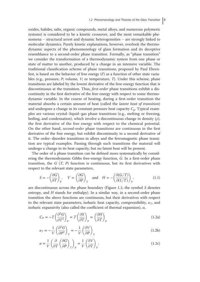
are discontinuous across the phase boundary (Figure 1.1; the symbol S denotesentropy, and H stands for enthalpy). In a similar way, in a second-order phasetransition the above functions are continuous, but their derivatives with respectto the relevant state parameters, isobaric heat capacity, compressibility, κT, andisobaric expansivity (also called the coefficient of thermal expansion), α,

CP � �T @2G

@T2

� �P

� T@S@T

� �P

� @H@T

� �P

(1.2a)

κT � � 1V

@2G

@P2

� �T

� � 1V

@V@P

� �T

(1.2b)

a � 1V

@

@T@G@P

� �T

� �P

� 1V

@V@T

� �P

; (1.2c)

1.2 Phenomenology and Theories of the Glass Transition 5

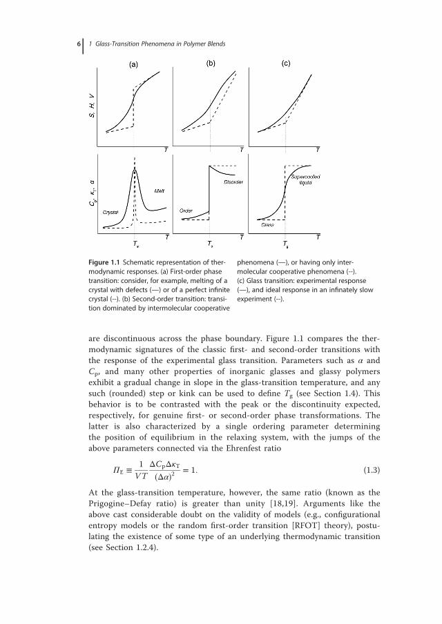
are discontinuous across the phase boundary. Figure 1.1 compares the ther-modynamic signatures of the classic first- and second-order transitions withthe response of the experimental glass transition. Parameters such as α andCp, and many other properties of inorganic glasses and glassy polymersexhibit a gradual change in slope in the glass-transition temperature, and anysuch (rounded) step or kink can be used to define Tg (see Section 1.4). Thisbehavior is to be contrasted with the peak or the discontinuity expected,respectively, for genuine first- or second-order phase transformations. Thelatter is also characterized by a single ordering parameter determiningthe position of equilibrium in the relaxing system, with the jumps of theabove parameters connected via the Ehrenfest ratio

ΠE � 1VT

ΔCpΔκT�Δα�2 � 1: (1.3)

At the glass-transition temperature, however, the same ratio (known as thePrigogine–Defay ratio) is greater than unity [18,19]. Arguments like theabove cast considerable doubt on the validity of models (e.g., configurationalentropy models or the random first-order transition [RFOT] theory), postu-lating the existence of some type of an underlying thermodynamic transition(see Section 1.2.4).

Figure 1.1 Schematic representation of ther-modynamic responses. (a) First-order phasetransition: consider, for example, melting of acrystal with defects (—) or of a perfect infinitecrystal (--). (b) Second-order transition: transi-tion dominated by intermolecular cooperative

phenomena (—), or having only inter-molecular cooperative phenomena (--).(c) Glass transition: experimental response(—), and ideal response in an infinately slowexperiment (--).


1.2.2

Structural, Kinetic, and Thermodynamic Aspects

One of the most intriguing questions in theoretical physics today is whether theglass is a new state of matter or just a liquid that flows too slowly to observe.The defining property of a structural glass transition for a polymer melt,observed on cooling from a sufficiently high temperature, is the increase of shearviscosity (η) by more than 14 orders of magnitude, without the development ofany long-range order in structure. The typical X-ray or neutron diffraction stud-ies of glassy solids, for example, reveal broad spectra of scattering lengths withno clear indication of primary unit cell structures. The “amorphous halo” of thestatic structure factor assessed by scattering experiments, or calculated viaMonte Carlo and molecular dynamics computer simulations of amorphous cells,also shows insignificant changes when the material crosses the glass transforma-tion range. Voronoi–Delaunay structural analyses of model amorphous systemshave provided some means for distinguishing subtle differences between therigid glass and liquid states of matter [12]. Relevant studies, however, areinconclusive as to the existence of some type of universally accepted geometricdescriptor of the feeble structural changes occurring during the transition.Contrary to the above findings, the marked change in behavior observed for

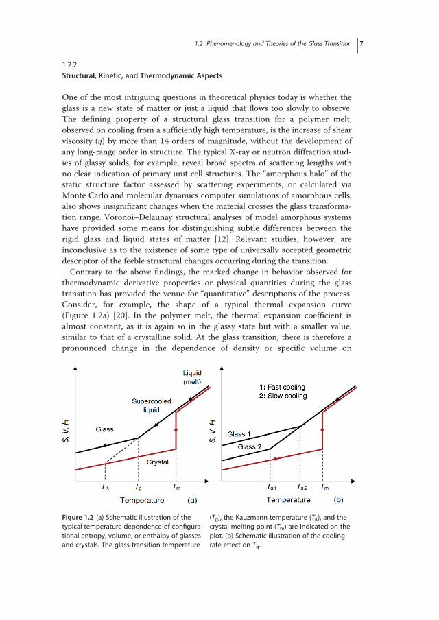
thermodynamic derivative properties or physical quantities during the glasstransition has provided the venue for “quantitative” descriptions of the process.Consider, for example, the shape of a typical thermal expansion curve(Figure 1.2a) [20]. In the polymer melt, the thermal expansion coefficient isalmost constant, as it is again so in the glassy state but with a smaller value,similar to that of a crystalline solid. At the glass transition, there is therefore apronounced change in the dependence of density or specific volume on

Figure 1.2 (a) Schematic illustration of thetypical temperature dependence of configura-tional entropy, volume, or enthalpy of glassesand crystals. The glass-transition temperature

(Tg), the Kauzmann temperature (TK), and thecrystal melting point (Tm) are indicated on theplot. (b) Schematic illustration of the coolingrate effect on Tg.


temperature; this constitutes the foremost identifier of the glass-transition tem-perature in all glass formers. Interestingly, the density of the glassy state and thelocation of the glass transition depend on the rate of temperature change,q= |dT/dt|. With reference to polymers, the sequence of chain conformationstates traversed during a slow cooling process exhibit reduced apparent volume(i.e., higher density), and this behavior extends to lower temperatures, relative tothe sequence of conformational states traversed at faster cooling. In parallel,since slower cooling rates allow for longer time for polymer chains to sampledifferent configurations (i.e., increased time for intermolecular rearrangement orstructural relaxation), the Tg decreases. The inflection point observed in theapparent volume, enthalpy, or entropy versus temperature plots of glass-formingmaterials marks the glass-transition temperature and demonstrates a similarcooling-rate dependence (Figure 1.2b). It is well known that variations in theheating rate produce similar effects, which are further complicated by additionalaspects of the kinetics of glassy behavior (structural recovery effects). All thesefeatures reveal that the value of Tg, unlike the melting temperature Tm, is a rate-dependent quantity, and that the transition defines a kinetically locked thermo-dynamically unstable state [21], or, otherwise, a metastable state of matter [22].Among other observations, the shape of the experimentally determined S(T)

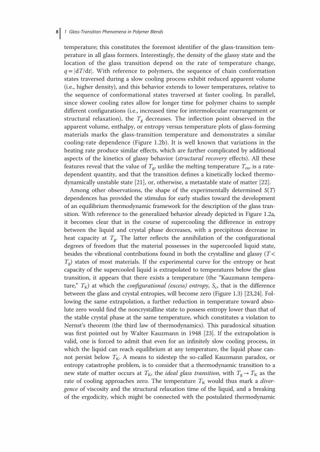
dependences has provided the stimulus for early studies toward the developmentof an equilibrium thermodynamic framework for the description of the glass tran-sition. With reference to the generalized behavior already depicted in Figure 1.2a,it becomes clear that in the course of supercooling the difference in entropybetween the liquid and crystal phase decreases, with a precipitous decrease inheat capacity at Tg. The latter reflects the annihilation of the configurationaldegrees of freedom that the material possesses in the supercooled liquid state,besides the vibrational contributions found in both the crystalline and glassy (T<Tg) states of most materials. If the experimental curve for the entropy or heatcapacity of the supercooled liquid is extrapolated to temperatures below the glasstransition, it appears that there exists a temperature (the “Kauzmann tempera-ture,” TK) at which the configurational (excess) entropy, Sc, that is the differencebetween the glass and crystal entropies, will become zero (Figure 1.3) [23,24]. Fol-lowing the same extrapolation, a further reduction in temperature toward abso-lute zero would find the noncrystalline state to possess entropy lower than that ofthe stable crystal phase at the same temperature, which constitutes a violation toNernst’s theorem (the third law of thermodynamics). This paradoxical situationwas first pointed out by Walter Kauzmann in 1948 [23]. If the extrapolation isvalid, one is forced to admit that even for an infinitely slow cooling process, inwhich the liquid can reach equilibrium at any temperature, the liquid phase can-not persist below TK. A means to sidestep the so-called Kauzmann paradox, orentropy catastrophe problem, is to consider that a thermodynamic transition to anew state of matter occurs at TK, the ideal glass transition, with Tg→TK as therate of cooling approaches zero. The temperature TK would thus mark a diver-gence of viscosity and the structural relaxation time of the liquid, and a breakingof the ergodicity, which might be connected with the postulated thermodynamic


transition. Experimental manifestation of the phenomenon is presumably maskedby the fact that, before getting to this temperature, the liquid falls out of equili-brium. Even so, it is a priori difficult to unequivocally interpret the glass-transitionphenomenon as a kinetic manifestation of a second-order transition due to theabsence of clear evidence showing growing thermodynamic or structural correla-tions as the system approaches the transition. Compelling evidence on the exis-tence of a static correlation function that displays a diverging correlation lengthrelated to the emergence of “amorphous order,” which would classify the glasstransition as a standard second-order transition, is still lacking [25]. Recent exper-imental results on equilibrated structures (see Section 1.2.3.1) cast doubt on thevalidity of the expectation of a dynamic divergence response, diverging timescales,and a concomitant singulatity in the thermodynamics at some temperature wellbelow laboratory Tgs.Considering the glass as a nonergodic, nonequilibrium, but slowly evolving

metastable state of matter, it is expected that its structure will undergo physicalprocesses that will progressively decrease its specific volume, enthalpy, or

Figure 1.3 Temperature dependence of theentropy difference between several supercooledliquids and their stable crystals at ambient pres-sure (ΔS/ΔSm, ΔSm being the entropy of fusion).The thick lines correspond to experimental datain the range between Tm (normal melting point)

and Tg. Extrapolation of the curve for lactic acidto lower temperatures is used to show the glasstransition and the Kauzmann temperatures (atthe point of intersection with the horizontalaxis). From ref. [24], with permission, 2001Nature Publishing Group.


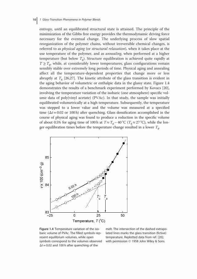
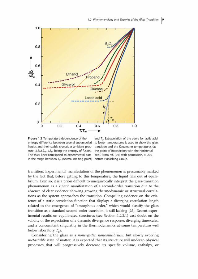
entropy, until an equilibrated structural state is attained. The principle of theminimization of the Gibbs free energy provides the thermodynamic driving forcenecessary for the eventual change. The underlying process of slow spatialreorganization of the polymer chains, without irreversible chemical changes, isreferred to as physical aging (or structural relaxation), when it takes place at theuse temperature of the polymer, and as annealing, when performed at a highertemperature (but below Tg). Structure equilibration is achieved quite rapidly atT �Tg, while, at considerably lower temperatures, glass configurations remainsensibly stable over extremely long periods of time. Physical aging and annealingaffect all the temperature-dependent properties that change more or lessabruptly at Tg [26,27]. The kinetic attribute of the glass transition is evident inthe aging behavior of volumetric or enthalpic data in the glassy state. Figure 1.4demonstrates the results of a benchmark experiment performed by Kovacs [20],involving the temperature variation of the isobaric (one atmosphere) specific vol-ume data of poly(vinyl acetate) (PVAc). In that study, the sample was initiallyequilibrated volumetrically at a high temperature. Subsequently, the temperaturewas stepped to a lower value and the volume was measured at a specifiedtime (Δt= 0.02 or 100h) after quenching. Glass densification accomplished in thecourse of physical aging was found to produce a reduction in the specific volumeof about 0.5% for aging time of 100h at T�Tg� 40 °C (Tg� 27 °C), while the lon-ger equilibration times before the temperature change resulted in a lower Tg.

Figure 1.4 Temperature variation of the iso-baric volume of PVAc. The filled symbols rep-resent equilibrium volumes, while opensymbols correspond to the volumes observedΔt= 0.02 and 100 h after quenching of the

melt. The intersection of the dashed extrapo-lated lines marks the glass transition (fictive)temperature. Replotted data from ref. [20];with permission 1958 John Wiley & Sons.


Since the measured volumes depend on the temperature and rate of coolingone can also talk about the “time” and “rate” of volume recovery. The rate ofvolume (or enthalpy) recovery depends on the magnitude and sign of the devia-tion from the reference equilibrium state, and on how long the sample wasallowed to remain at the preceding temperature (memory effect). Plain kineticeffects can be described using a simple kinetic theory, like the single-parametervolume (or enthalpy) relaxation model proposed by Tool [28], and Davies andJones [29],

� dδvdt

� qδα � δvτv; (1.4a)

where δv = (V�Veq)/Veq, Veq is the equilibrium state volume, and τv is the iso-baric volume relaxation time. This model was later improved using the Doolittleequation, resulting in

� dδvdt

� qΔα � δvδvg

expBf g

� Bf

!; (1.4b)

where τvg is a reference relaxation time and fg the free-volume fraction at Tg. Toaccount for the memory effects, the superposition of a number of elementaryrelaxation processes has been considered in the multiparameter Kovacs–Aklo-nis–Hutchinson–Ramos approach [30],

� dδv;idt

� qΔαi � δv;iτv;i

(1.4c)

with δv �PNi�1 δv;i and Δα �PN

i�1 Δαi. Enthalpy relaxation effects on differentialscanning calorimetry (DSC) heating scans (Section 1.4.1) are most prominentwhen the material is isothermally held in the glassy state (20°–50° below Tg), fora sufficient duration of time. In addition to rate effects, the glass transition ispressure and path dependent. McKenna and Simon [14] reviewed studies relatedto the path dependence of Tg and the kinetics of glass formation. Their surveyclearly demonstrates that the glass-transition temperature and its pressuredependence are functions of whether the PVT surface of the glass is obtainedisobarically, by pressurizing the liquid and cooling from above Tg, or isochori-cally, using variable pressure to retain liquid volume constant until a low tem-perature is reached at a constant rate.

1.2.3

Relaxation Dynamics and Fragility

The relaxation dynamics in many different kinds of materials encompass contri-butions from various types of motional processes spanning a range of lengthscales, which become prominent at different temperature ranges and/or time-scales. By virtue of their high densities, supercooled liquids exert strong frustra-tion constraints on the dynamics of individual atomic/molecular entities or


“particles” (e.g., atoms, oligomeric molecules, pendant groups, short-chain seg-ments, or even bigger parts of the chain). As temperature decreases toward Tg, atagged particle is most likely trapped by neighbors (i.e., caged) given that theamplitude of thermodynamic fluctuations decreases following a decrease in tem-perature. Near the glass-transition temperature, several groups of particles mayremain caged for relatively long times. For them, liberation from the cagerequires collaborative rearrangement of several other particles in its environ-ment, which themselves are also imprisoned. The volume over which cagerestructuring – by cooperative motions – must occur presumably increases asthe molecular packing increases (with decreasing temperature). Considering thecomplexity of the systems involved and the diversity of configurational changesthat may cause relaxation of a polymeric material, fundamental research in eachsystem often focuses on the description of the time evolution of the relaxationdynamics (i.e., plots of the time dependence of the relaxation or response func-tions), at a constant temperature, and the creation of relaxation maps (i.e., plotsof the temperature dependence of the relaxation times of distinct groups of par-ticles). Some of these issues and the pertinent concept of liquid fragility will bebriefly discussed.

1.2.3.1 Relaxations in Glass-Forming MaterialsFor over half a century, the nature of the relaxational response of supercooledliquids and glasses has been extensively explored, in an effort to expand ourunderstanding of the structure–property relationships in the rapidly evolvingcollection of glassy materials, and at the same time establish connections amongexperimental responses and theoretical predictions. Out-of-equilibrium studiesof glassy dynamics reveal a collection of modes, extending over a broad tempera-ture-, frequency-, or time range. At short times of observation at constant tem-perature, the approach to equilibrium after a given perturbation is dominated byvery fast to moderately fast motions of small parts of the macromolecular chain.The picosecond dynamics of disordered materials include a fast secondary relax-ation process, which appears as an anharmonic relaxation-like signal (a broadquasielastic scattering) in the GHz–THz region of excitation spectra [31]. Thiscontribution is commonly ascribed to caged molecular dynamics (i.e., cage rat-tling) with relaxational activity displaying gas-like power-law temperature depen-dence [32]. Close to it, Raman and neutron scattering inelastic studies reveal arather controversial lower frequency vibrational mode, or group of modes,known collectively as the “boson peak.” Potential correlations between theseearly-time modes and the long-time dynamics of glass-forming materials emergefrom studies relating characteristics (e.g., its intensity and frequency) of thenearly temperature-independent boson peak with the concept of liquid fragility,Kohlrausch’s exponent (βKWW) [33], and the cooperativity length scale (ξα) [34],all strongly linked to the glass-transition dynamics of disordered media. Severalother important secondary processes occur on timescales much slower than cagerattling, but much faster than the structural (α) relaxation. These are related tocomplicated, though local, non or not fully cooperative [35] dynamics. A number


of physical origins have been proposed for the principal slow secondary relaxa-tion process (in the kHz region of isothermal relaxation spectra [15–17]), the so-called Johari–Goldstein (JG) β-process, a process widely recognized as an intrin-sic feature of the glassy state and frequently deemed to originate from the samecomplicated frustrated interactions leading to the glass transition. Of the alterna-tive attributions proposed hitherto, it is worth mentioning its correlation withmolecular motions occurring in “islands of mobility” (i.e., regions of relativelyloose structure [36]), the highly restricted stepwise reorientation of practically allmolecules in a system [37], and its discussion in terms of intermolecular [38]degrees of freedom or even intramolecular [39] ones. Other secondary relaxa-tions (γ or δ, in the accepted notation for amorphous materials [15,16]) entailmore trivial and system-specific motions of structural entities, usually connectedwith intramolecular degrees of freedom, such as simple bond rotations of lateralgroups (including rotations within side groups). With the exception alreadynoted for the modes contributing to the fast (picosecond) dynamics of disor-dered materials, all other secondary mechanisms are commonly regarded toinvolve relaxation jumps over asymmetric double-well potentials (e.g., Gilroy–Phillips model [40]). The temperature dependence of the respective relaxationtimes can thus be well described by a simple exponential Arrhenius-type equa-tion, that is,

τ�T � � τ0 expEact

kβT

� �; (1.5)

where τ0 is the pre-exponential factor (or Arrhenius prefactor) and kβ is theBoltzmann constant. The apparent activation energy, Eact, is typically determinedby internal rotation barriers (intramolecular part) and the environment of therelaxing unit (intermolecular part, linked to the stereochemical configuration ofthe chains). Broad distributions of relaxation times and a strongly temperature-dependent width (presumably due to a Gaussian distribution of barrier heights)are common features of signals related to the JG mode [41]. In several cases, byextrapolating to high temperatures the Arrhenius line, the slow β-mode seems toresult from bifurcation of the structural relaxation mode (α-relaxation,Figure 1.5), which encompasses cooperative segmental motions on much longerlength scales.The abrupt retardation of molecular mobility in the course of vitrification is an

important facet of the relaxation dynamics of disordered systems. Various exper-imental results and simulations indicate that the structural relaxation of a super-cooled liquid is a dynamically and spatially heterogeneous process with astrongly non-Arrhenius relaxation behavior. Dynamic heterogeneity describesthe spatial heterogeneity of the local relaxation kinetics, manifested by thecoexistence of “slow” and “fast” mobility regions of limited length within a mate-rial [42–44]. Different assumptions that introduce heterogeneity in supercooledliquids exist, including the old concept of liquid-like cells that create liquid-likeclusters (Cohen–Crest model), the conception of a solid glass with a small frac-tion of fluidized domains of extremely high mobility (Stillinger–Hodgdon


model), and the hypothesis of the existence of small distinguishable subvolumesin the system that relaxes statistically independent of their environment. Theterminology germane to these regions includes the influential “cooperativelyrearranging region(s)” (CRR(s)) introduced in the Adam–Gibbs model, the con-cept of “entropic droplets,” and the “domains” of locally preferred structures,advocated by thermodynamic treatments of glass formation (see Section 1.2.4.3).So far, most techniques provide indirect estimates of the relevant cooperativitylength scale, by invoking thermodynamic fluctuation formulae, combined withan appropriate set of ad hoc assumptions, to obtain ξα from the available exper-imental data, or by simply introducing external perturbations (e.g., confinementin finely regulated nanometer-sized geometries) [43,45–47]. In the subvolume ofeach CRR, for example, the density, the temperature, the entropy, and the energy(E) are somewhat different, and their mean square fluctuations hΔρ2i, hΔT2i,hΔS2i, and hΔE2i, respectively, are given by standard relations of statistical ther-modynamics. Among others [47], Donth proposed to correlate these relationswith the width of relaxation time distribution of the so-called α-relaxation pro-cess [41]. Each subvolume can be then considered as a thermodynamic system inmetastable equilibrium with fluctuating variables having a Gaussian distribution,and a distinct glass-transition temperature (Tα) and relaxation time (τα). Accord-ingly, the relaxation time distribution can be related to the glass transition one,

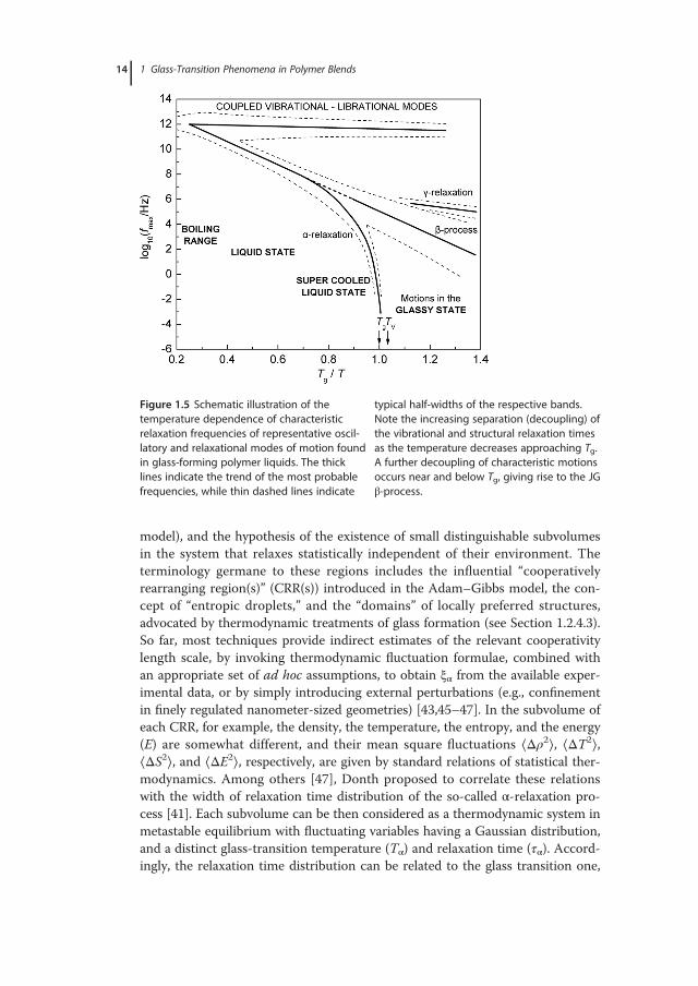
Figure 1.5 Schematic illustration of thetemperature dependence of characteristicrelaxation frequencies of representative oscil-latory and relaxational modes of motion foundin glass-forming polymer liquids. The thicklines indicate the trend of the most probablefrequencies, while thin dashed lines indicate

typical half-widths of the respective bands.Note the increasing separation (decoupling) ofthe vibrational and structural relaxation timesas the temperature decreases approaching Tg.A further decoupling of characteristic motionsoccurs near and below Tg, giving rise to the JGβ-process.


with hTαi assumed to be the conventional glass-transition temperature of thesystem. In Donth’s approach, the characteristic volume of cooperativity at Tg

(Vα) and the number of segments in the cooperative volume (Nα) can be esti-mated by

V α ∝ ξ3α � Δ�1=CV �ρ�δT �2 kBT

2g (1.6a)

and

Nα � ρNAξ3α

M0; (1.6b)

respectively, with NA the Avogadro number, (δT)2 the mean square temperaturefluctuation related to the dynamic glass transition of a CRR, Cv the isochoricheat capacity with Δ(1/Cv)�Δ(1/Cp)= (1/Cp)glass� (1/Cp)liquid, and M0 the molarmass of the repeat unit (monomer). Theoretical claims [46], thermodynamictreatments starting from volume, temperature, and entropy fluctuations [41,47],and extensive use of sensitive experimental probes of dynamic and spatial het-erogeneity [43,47] – including results based on the Boson peak frequency [34] –have provided values for ξα in the range ∼1–4 nm [35]. In parallel, the coopera-tivity length scale and Nα (of the order of 100 near Tg) appear to increase astemperature decreases near Tg [31].The strongly non-Arrhenius temperature behaviors for the structural relaxation

dynamics and the viscosity of glass-forming liquids at temperatures exceeding Tg

are well documented (Figure 1.5). Both are frequently interpreted in terms of theempirical Williams–Landel–Ferry (WLF) [48] or Vogel–Fulcher–Tammann–Hesse (VFTH) [49] equations, which were later rationalized in terms of free-vol-ume (or configurational-entropy) concepts. The WLF equation is expressed as

log10 αT � �C1�T � T r�C2 � �T � T r� ; (1.7a)

where αT is called the temperature shift factor (generally known as the reducedvariables shift factor), Tr is a reference temperature, and C1 and C2 are constants.The shift factor is related to the viscosity, αT= η(T)/η(Tr), relaxation times, αT=τ(T)/τ(Tr), and several other mechanical (e.g., tensile strength and compliance)or dielectric (e.g., permittivity and electric modulus) relaxing quantities. WhenTg is taken as the reference temperature, the following form is obtained:

log10 αT � �17:44�T � T g�51:6 � �T � T g� : (1.7b)

By averaging data for various types of synthetic high polymers, the values ofC1= 17.44 and C2= 51.6K were derived and applauded as “universal” constantsfor linear amorphous polymers of any chemical structure. Their usability in com-plex polymeric systems must be treated with cautiousness, since a different set ofvalues is to be expected when distinct dynamic processes and/or substances areexplored. Despite these shortcomings, Eq. (1.7b) introduces some important


kinetic aspects of the glass-transition phenomenon. For instance, if the time frameof an experiment is decreased by a factor of 10 near Tg, this equation reveals anincrease of the glass-transition temperature of about 3°. Of particular interest indynamic experiments is the temperature dependence of the structural α-relaxa-tion times, τα(T), for which the WLF temperature dependence is expressed as

τα�T � � τ�T r�exp �C1�T � T r�C2 � �T � T r��

(1.8)

and the mathematically equivalent VFTH equation has the form

τα�T � � τ 1� �exp CT � TV

� �; (1.9)

where C � C1�T r � TV� is a material parameter and TV � T r � C2 denotes theso-called Vogel temperature (at which the relaxation time is extrapolated todiverge). In the absence of deep arguments regarding the underlying physics ofglasses, the VFTH equation is mostly regarded an entirely heuristic modificationof the Arrhenius rate law to include a finite divergence temperature. Eventhough the physical meaning of the Vogel temperature has not been clearlydefined [41], the universality of the VFTH equation in a wide temperature range(Tg to Tg+ 100K) makes clear that TV is a significant parameter for the dynam-ics of the glass transition. A survey of the literature provides evidence of a weakconnection between TV and TK (TV�TK [50]), with TV generally found to beapproximately 30°–50° (depending on system’s fragility) below conventional lab-oratory Tgs. In practice, the glass-transition temperature can be obtained byextrapolating the Arrhenius plot constructed for the structural relaxation timesor characteristic frequencies (plots of log τ or log fmax versus 10

3/T, with fmax= 1/2πτ), using Eq. (1.8) or (1.9) along with the usual convention τ(Tg)= 100 s [51].Theoretical treatments, computer simulations, and a number of experimental

results strongly argue in favor [52] or against [53–55] the existence of a dynamicdivergence phenomenon – a behavior also referred to as “super-Arrhenius” – atsome temperature above absolute zero. The “geological” ages required for amaterial to attain equilibrium far below Tg preclude, in general, extensive testingof the above conjecture. Recent data on the temperature dependence of the shiftfactor obtained by dielectric spectroscopy for PVAc [54], using samples aged toequilibrium as much as 16° below the calorimetric glass-transition temperature,demonstrate, for example, an Arrhenius sub-Tg behavior in contradiction to thepredictions made by classic theories. Further work on a Cenozoic (20 millionyears old) Dominican amber [55] was able to probe equilibrium dynamics nearly44° below Tg, and subsequently present more stronger experimental evidence ofnondiverging dynamics at far lower temperatures than previous studies. Noticethat several other functions may well provide adequate description of the super-Arrhenius behavior of glass-forming liquids, showing either a divergence at zerotemperature (e.g., the Bässler-type law, τα(T)∼ exp(A/T2) [56]) or no divergenceat all (e.g., the DiMarzio–Yang formula, τα(T)∼ exp(�AFc/kβT), where Fc is theconfigurational part of the Helmholtz free energy [57]).


1.2.3.2 The Concept of FragilityIn an attempt to establish some link between the observed thermodynamicbehaviors of glass-forming systems and the temperature dependences of severaldynamical quantities, Angell introduced the concept of liquid fragility [58]. InAngell’s classification scheme, the word “fragility” is used to characterize therapidity with which a liquid’s properties (such as η(T) or τ(T)) change as theglassy state is approached, in contrast to its colloquial meaning that most closelyrelates to the brittleness of a solid material. Over the years, fragility has become auseful means of characterizing supercooled liquids, despite the criticism on someinferences of the concept [59]. The term “strong” liquid suggests a system withrelatively stable structure and properties (such as the activation energy barriersassociated with viscosity or the structural relaxation time) that do not changedramatically in going from the liquid into the glass, while a “fragile” liquidbehaves in a reverse manner. Formally, fragility reflects to what degree the tem-perature dependence of a dynamic property of the glass former deviates from theArrhenius behavior. One way of evaluating fragility is to construct fragilityplots (Angell plots), where the logarithm of a dynamical quantity is plotted ver-sus Tg/T (Figure 1.6) [60]. Several parameters have been introduced, at differenttheoretical contexts and with varying level of success, for characterizing quanti-tatively the fragility of glass-forming liquids (e.g., see treatments of Doremus [59],Bruning and Sutton [61], and Avramov [62]). The most common definition offragility is the fragility parameter (or steepness index), m, which characterizesthe slope of a dynamic quantity (X) with temperature as the material approachesTg from above [63],

m � @ log10X@�T g=T ��

T�Tg

: (1.10)

Bearing in mind the non-Arrhenius temperature dependence of τα, for example,Eq. (1.10) takes the form

mVFTH � @ log10 τα@�T g=T �

� �T�Tg

� C=T g

�ln 10� 1 � TV

T g

� �2 ; (1.11a)

which provides an estimate of the fragility index in terms of the Vogel tempera-ture. Considering the expression of the relaxation time given by the Tool–Narayanaswamy–Moynihan formula [28,64], another dynamic estimate of thefragility index can be obtained from DSC experiments with different heatingrates, through a relation that links m with the apparent activation energy ofstructural relaxation Δh∗,

mDSC � Δh�RT g ln 10

: (1.11b)

The fragility can be intuitively related to the cooperativity of atomic motionsin the glassy state (anticipating an increase in cooperativity with increasing m)


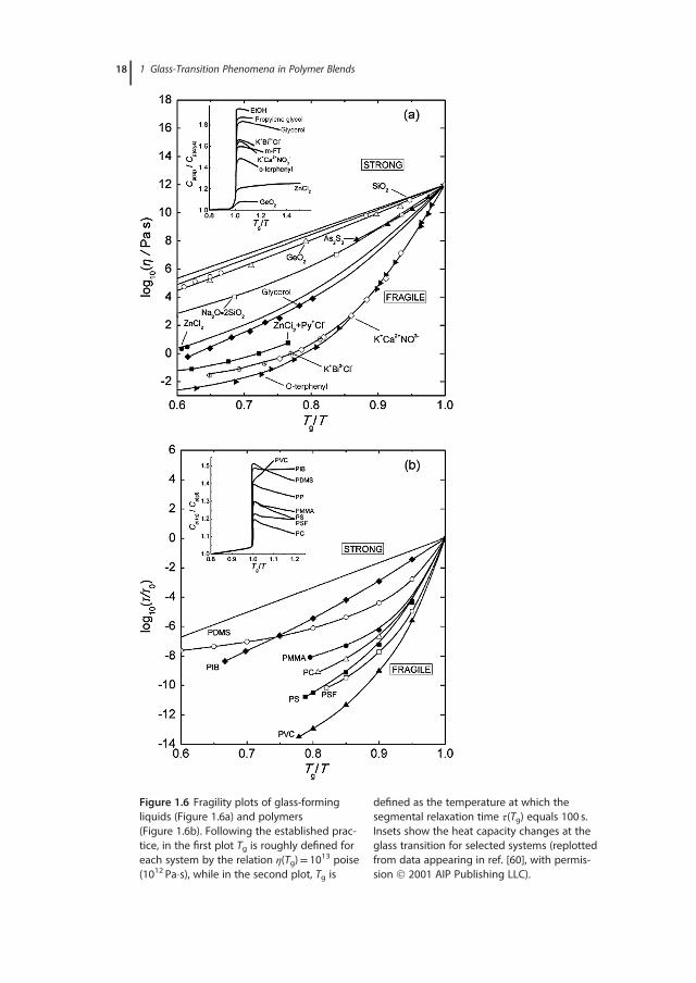
Figure 1.6 Fragility plots of glass-formingliquids (Figure 1.6a) and polymers(Figure 1.6b). Following the established prac-tice, in the first plot Tg is roughly defined foreach system by the relation η(Tg)= 1013 poise(1012 Pa�s), while in the second plot, Tg is

defined as the temperature at which thesegmental relaxation time τ(Tg) equals 100 s.Insets show the heat capacity changes at theglass transition for selected systems (replottedfrom data appearing in ref. [60], with permis-sion 2001 AIP Publishing LLC).


[41,45], as well as to the breakdown of the Stokes–Einstein relation between vis-cosity and diffusion coefficient [65]. In that respect, several studies explore thevalidity of empirical relationships among components of the fragility parame-ter [34,66] and the length scale of cooperativity or spatial variations in dynamics.For example, by applying the chain rule of differentiation

m � @ log10 τα

@T g

T

� �0BB@

1CCA

P

��T�Tg

� @ log10 τα

@T g

T

� �0BB@

1CCA

V

��T�Tg

� @ log10 τα@P

� �T

��T�T g

� @P

@T g

T

� �0BB@

1CCA

V

��T�Tg

one separates the conventional (isobaric) fragility parameter into two terms

m � mV � ΔV #

kB ln 10� αTκT

(1.12)

with ΔV# denoting the activation volume at Tg. Following the above treatment,Sokolov and coworkers [34] suggested that the isochoric (constant density) fra-gility, mV, characterizes the pure thermal contribution to fragility that bears noconnection to the length scale of dynamic heterogeneities. The second term ofEq. (1.12) encompasses the volume contribution to fragility, that is, the effectdue to the temperature-induced change of density under isobaric conditions.Given the correlation evidenced between the cooperativity volume ξ3α andΔV# [34], this term is likely to depend directly on cooperativity. A relationshipbetween parameters characterizing the stretching of the relaxation function andisochoric fragility is also probable [66]. Other studies provide pieces of evidencefor possible correlations between the conventional (atmospheric pressure) esti-mates of the fragility parameter and molecular or structural properties of thematerial, such as its chemical composition, the type of bonding, intermolecularinteractions, or the degree of microphase separation [67].The values of m range from ∼250 [68] for very fragile glass-forming liquids

(e.g., ionic systems, organic materials, or polymers with nondirectional inter-molecular bonding) to the theoretically low limit of ∼16 [69] for very strongglass formers (the network oxides SiO2 and GeO2, BeF2, etc. [70]). Highly fragilematerials demonstrate narrow transitions, while those with lower fragility indiceshave relatively broader transitions. The roles of chemical structure, composition,and main-chain stiffness in the glass-forming tendency of polymers [71] andpolymer blends [51], as well as possible correlations among the “dynamic fragil-ity” index and thermodynamic measures of liquid fragility (mT=ΔCp, Cp(liq)/Cp

(gl), Cp(liq)/Cp(crys), or 1+ΔCp/Sc, all determined at T=Tg, typically used to assert“thermodynamic fragility” [60,72]), are issues in debate [73]. As suggested by theAdam–Gibbs theory (see Section 1.2.4), kinetically fragile liquids are expected tohave large configurational heat capacities [6], resulting from their configurational


entropy changing rapidly with temperature. Strong glass-forming liquids areresistant to temperature-driven changes in the medium-range order. Therefore,the amount of configurational entropy in the liquid is small, as is the change inheat capacity at Tg. Even though the heat capacity changes shown in the inset ofFigure 1.6a support the positive correlation between m and ΔCp, more recentdata appear contradicting. Huang and McKenna [60] classified the experimentalm versus ΔCp dependences into three groups: polymeric glasses with a negativecorrelation (Figure 1.6b) [72], small-molecule organics and hydrogen-bondingsmall molecules with no correlation, and inorganic glass formers with a positiveone [74]. There are also several reports demonstrating that thermodynamic andkinetic fragilities are not strongly correlated [75], especially when polymeric sys-tems are considered. In view of that, a system concluded to be kinetically fragilewill not necessarily be also thermodynamically fragile. Finally, a direct correla-tion between fragility indices and the average size of the CRRs is frequentlyconsidered [41,45,76].

1.2.4

Theoretical Approaches to the Glass Transition

1.2.4.1 General OverviewThe intriguing phenomenology of the glass transition has been the driving forceof intense efforts aiming to establish firm theoretical perspectives with widequantitative support for the microscopic and relaxational behavior of liquids inthe glass transformation range. The marked decrease in molecular mobility as asystem passes through its glass-transition temperature has led several research-ers to construct early theories of glass transition based on concomitant changesof conjugate thermodynamic variables, such as the free volume and the configu-rational entropy. The defect diffusion [77], free volume [78], and configurationalentropy [44,79,80] approaches, all dating back to the 1960s, remain in the fore-front of current interest about the glass transition. While these early theories fallshort in properly defining – among other properties and phenomena – themolecular motions involved in the glass-transition mechanism [13], they are stillfrequently invoked in interpretations of experimental results. A number of morerecent theories and elaborate concepts, including the potential energy landscape(PEL) picture [24,81,82], the coupling model (CM) [13], the mode-coupling the-ory (MCT) [83–85], and the RFOT [86] theory, the configuron percolationmodel (CPM) [87–89], as well as the concepts of kinetic constraints [90,91] andgeometric frustration [92], have provided an amplification of our perceptions onthe glass-transition phenomenon and more plausible explanation of certainexperimental observations. Still, irrespective of the intense theoretical efforts tohandle the glass-transition phenomenon employing arguments resembling ther-modynamic or purely dynamic transitions, we have not yet arrived at a compre-hensible theory of supercooled liquids and glasses. Their behavior near the glasstransition has been described, but not all that behavior is thoroughly explainedby a single theoretical concept [85]. Elements of certain theoretical frameworks


and some insight into their strengths, flaws, capabilities, and limitations will beprovided in the following paragraphs; the reader is referred to a – regretfullycondensed – list of review papers [13,25,85,93–95] for a comprehensive accountof the available theoretical approaches.

1.2.4.2 Energy Landscapes and Many-Molecule Relaxation DynamicsIn a seminal 1969 paper, Goldstein [81] put forward the notion that atomicmotions in a supercooled liquid comprise high-frequency vibrations in regionsof deep potential energy minima in addition to less frequent transitions to othersuch minima. In an amplification of this concept, Stillinger and coworkers [24,82]formulated the PEL picture of glassy systems, a multidimensional surfacedescribing the dependence of the potential energy on the coordinates of theatoms or molecules. Their conception provided a “topographic” view of phe-nomena associated with glass formation, along with a valuable theoretical back-ground in the pursuit of distinguishing among vibrational and configurationalcontributions to the properties of a viscous fluid.In the phenomenological PEL approach of Stillinger and Weber [24], an

N-particle system is represented by a potential energy function U(~r 1;~r 2; . . . ;~r N )in the 3(N � 1)-dimensional configuration space. The energy of the disorderedstructure is partitioned into a discrete set of “basins” connected by saddle points– a picture that represents the complicated dependence of potential energy (orenthalpy) on configuration [96]. Each basin contains a metastable local (single)energy minimum and each corresponds to a mechanically stable arrangement ofthe system’s particles. In terms of PEL, relaxations ascribed to short-time molecu-lar motions are considered to occur via intrabasin vibrations (harmonic oscilla-tions) about a particular structure, while long-time molecular motions areconsidered to take place via occasional activated jumps over saddle points intoneighboring basins. In an amplification of this concept, the picture of “metaba-sins” has been introduced [97], with each metabasin consisting of several localminima (“inherent structures”) separated by similar low-energy barriers. Jumpswithin the superstructure of a metabasin are connected with secondary relaxationevents (Figure 1.7a), while much slower collective molecular motions (i.e., “ergo-dicity restoring” processes related to the glass transition) are considered to pro-ceed via infrequent jumps between neighboring metabasins, separated by largebarriers relative to kβT. While the PEL is suitable for modeling glass-transitionbehavior under isochoric conditions, almost all experimental studies of glass for-mation are performed under constant pressure conditions. To that end, anenthalpy landscape approach [98] has conveyed an extension of PEL to an iso-thermal–isobaric ensemble, allowing for changes in both particle positions andthe overall volume of the system. In all energy landscape models (potential-energy, free-energy, or enthalpy variants [97,98]), the dynamics are to a certaindegree cooperative, since transitions between two minima engage the coordinatesof all particles of some localized region. Related frameworks have contributed acertain degree of understanding of the nature of the glass transition and the glassystate of matter. It has been suggested, for example, that it is not possible for the


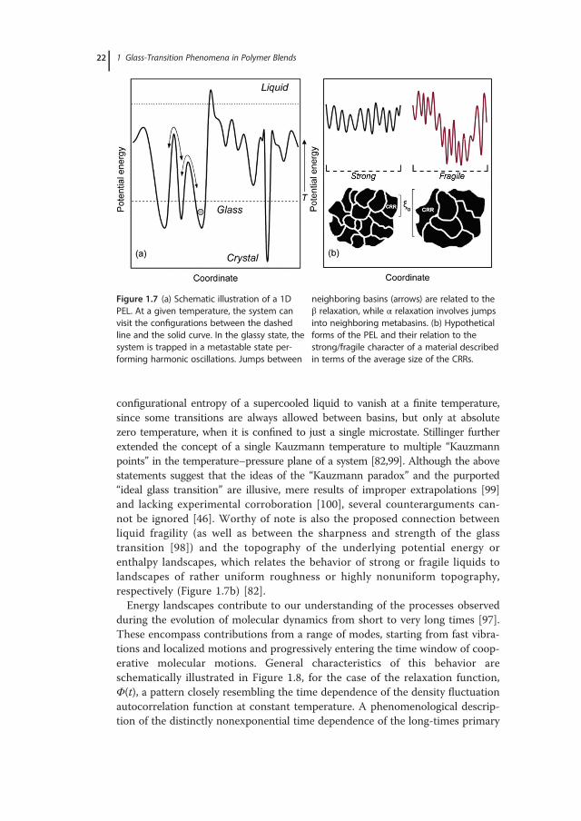
configurational entropy of a supercooled liquid to vanish at a finite temperature,since some transitions are always allowed between basins, but only at absolutezero temperature, when it is confined to just a single microstate. Stillinger furtherextended the concept of a single Kauzmann temperature to multiple “Kauzmannpoints” in the temperature–pressure plane of a system [82,99]. Although the abovestatements suggest that the ideas of the “Kauzmann paradox” and the purported“ideal glass transition” are illusive, mere results of improper extrapolations [99]and lacking experimental corroboration [100], several counterarguments can-not be ignored [46]. Worthy of note is also the proposed connection betweenliquid fragility (as well as between the sharpness and strength of the glasstransition [98]) and the topography of the underlying potential energy orenthalpy landscapes, which relates the behavior of strong or fragile liquids tolandscapes of rather uniform roughness or highly nonuniform topography,respectively (Figure 1.7b) [82].Energy landscapes contribute to our understanding of the processes observed

during the evolution of molecular dynamics from short to very long times [97].These encompass contributions from a range of modes, starting from fast vibra-tions and localized motions and progressively entering the time window of coop-erative molecular motions. General characteristics of this behavior areschematically illustrated in Figure 1.8, for the case of the relaxation function,Φ(t), a pattern closely resembling the time dependence of the density fluctuationautocorrelation function at constant temperature. A phenomenological descrip-tion of the distinctly nonexponential time dependence of the long-times primary

Figure 1.7 (a) Schematic illustration of a 1DPEL. At a given temperature, the system canvisit the configurations between the dashedline and the solid curve. In the glassy state, thesystem is trapped in a metastable state per-forming harmonic oscillations. Jumps between

neighboring basins (arrows) are related to theβ relaxation, while α relaxation involves jumpsinto neighboring metabasins. (b) Hypotheticalforms of the PEL and their relation to thestrong/fragile character of a material describedin terms of the average size of the CRRs.


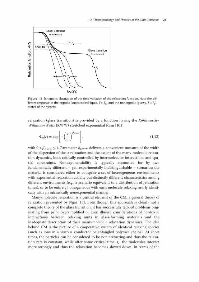
relaxation (glass transition) is provided by a function having the Köhlrausch–Williams–Watts (KWW) stretched exponential form [101]

Φα�t� � exp � tτα

� �βKWW

" #; (1.13)

with 0< βKWW� 1. Parameter βKWW delivers a convenient measure of the widthof the dispersion of the α-relaxation and the extent of the many-molecule relaxa-tion dynamics, both critically controlled by intermolecular interactions and spa-tial constraints. Nonexponentiallity is typically accounted for by twofundamentally different – yet, experimentally indistinguishable – scenarios: thematerial is considered either to comprise a set of heterogeneous environmentswith exponential relaxation activity but distinctly different characteristics amongdifferent environments (e.g., a scenario equivalent to a distribution of relaxationtimes), or to be entirely homogeneous with each molecule relaxing nearly identi-cally with an intrinsically nonexponential manner.Many-molecule relaxation is a central element of the CM, a general theory of

relaxation presented by Ngai [13]. Even though this approach is clearly not acomplete theory of the glass transition, it has successfully tackled problems orig-inating from prior oversimplified or even illusive considerations of nontrivialinteractions between relaxing units in glass-forming materials and theinadequate description of their many-molecule relaxation dynamics. The ideabehind CM is the picture of a cooperative system of identical relaxing species(such as ions in a viscous conductor or entangled polymer chains). At shorttimes, the particles can be considered to be noninteracting and thus the relaxa-tion rate is constant, while after some critical time, tc, the molecules interactmore strongly and thus the relaxation becomes slowed down. In terms of the

Figure 1.8 Schematic illustration of the time variation of the relaxation function. Note the dif-ferent response in the ergodic (supercooled liquid, T> Tg) and the nonergodic (glassy, T< Tg)states of the system.


CM, the characteristics of the structural relaxation are correlated with theaspects of the processes that have transpired before it, which include the cagingof the molecules (picosecond dynamics) and the universal JG β-process [36]. Arational outcome of the notion that the α-relaxation process originates from therelaxation of individual molecules is to consider that, at sufficiently short times,the many-molecule relaxation is reduced to isolated local motions independentof each other. These correspond to the primitive relaxation of the CM, whichcan be seen as part of the faster processes in the relaxation spectrum. The modelsets forth a relation between τα and the primitive relaxation time (τp), orequivalently the JG relaxation time (τJG), via the coupling parameter n (withn= 1� βKWW) characterizing the primary relaxation, of the form [13]

τα�T ;P� � t�nc τp�T ;P�� 1=�1�n� � t�nc τJG�T ;P�� 1=�1�n�: (1.14)

The CM predicts the short-time behavior to be essentially Debye. Although thetemperature and pressure dependences of τα and τp (or τJG) are not given orderived, the applicability of Eq. (1.14) has been successfully tested for a widerange of glass formers. The stronger dependence of τα(T, P) compared to that ofτp(T, P) or τJG(T, P) is expressed by the superlinear factor 1/(1�n) and relates tothe longer length scale of the motions involved. The CM also provides an explan-ation of changes in the relaxational behavior of glass formers – including thecomponent dynamics of mixtures or the dynamics of nanoconfined polymers –in terms of the temperature dependence of n or the width of the α-relaxation. Ofthe cases compiled by Ngai [13], here is only mentioned the projected crossoverof the temperature dependence of τα from one VFTH equation to another, atsome temperature TB>Tg, coincident with the apparent onset of bifurcation ofτJG from τα, and the onset of decoupling of the translational and orientationalmotion, which are all related to the small values of n at T>TB and its more rapidincrease with decreasing temperature below TB. Ngai and Rendell [13] mentionthat an explanation of the heterogeneous picture of relaxation in terms of spectraor distributions of relaxation times is incompatible with the model. They arguethat interactions perturb the relaxation in a way as to make it inherently nonex-ponential and not that it arises from superposition of single exponential (Debye)processes. A main limitation of the CM is connected with the absence of adetailed explanation of the potential relaxation mechanisms in molecular leveland how these exactly contribute to the overall macroscopic behavior.

1.2.4.3 Approaches with an Underlying Avoided Dynamical TransitionThe most famous purely dynamical approach to the glass transition is the MCT, amean-field treatment of the phenomenon based on a microscopic theory of thedynamics of fluids [83–85]. The theory exploits the idea of a nonlinear feedbackmechanism in which strongly coupled microscopic density fluctuations lead tostructural arrest and diverging relaxation time at a critical point, with no singular-ity observed for the thermodynamics. The physical picture adopted by the origi-nally developed scenario of the idealized MCT (iMCT) attributes the viscousslow-down with decreasing temperature to a so-called cage effect, that is, the


assumption that each particle in a dense fluid is kinetically constrained (confined)in a cage formed by neighboring particles. At low temperatures, the probability ofoccurrence of a strong spontaneous density fluctuation, large enough to liberate aparticle from its cage, appears insignificant. In consequence, as the temperaturegets lower and the system gets denser, structural arrest occurs because particlescan no longer leave their cage even at infinite time. Within the MCT, fast second-ary relaxations are related to relatively rapid local motions of molecules trappedinside cages, while the slow process of the breakup of a cage itself contributes tothe structural relaxation. Large-scale spatial motion typical of a fluid can only pro-ceed cooperatively, that is, one of the caging particles has to make way, which canonly happen if one of its neighbors moves, and so on. One of the main predic-tions of the iMCT is that dynamical freezing and a transition from an ergodic toa nonergodic state occurs at a critical temperature TMCT (∼1.2Tg). Above TMCT,where ergodicity is obeyed, all regions of phase space are accessible, while belowTMCT, where structural arrest occurs, parts of phase space remain inaccessible.At T=TMCT, the iMCT visualizes the “self” part of the intermediate scatteringfunction, Fs(k, t), to decay (in the limit t→1) to a finite, nonzero, number calledthe nonergodicity parameter. For temperatures exceeding TMCT, the iMCT pre-dicts that the scattering function decays to zero in two steps (β- and α-regimes),with the decay of the correlation function at long times approximated by thestretched exponential KWW function (see Figure 1.8). Approaching TMCT fromabove, the structural relaxation time (and viscosity) scales in a power-law fashion

τα�T �∝ T � TMCT� ��γ ; (1.15)

where TMCT is a critical temperature for the onset of the glass transition, and theexponent γ > 1.5.The idealized mode-coupling approach successfully describes key aspects of

the relaxation dynamics of moderately supercooled liquids, with its mainachievement involving the prediction of the two-step relaxation process thatemerges as temperature decreases, in agreement with experimental studies andsimulation results. Nevertheless, the dynamic arrest and the predicted singularityat the purported critical temperature of the model bear no connection to thelaboratory glass transition or a transition to an “ideal” glass state of matter.Experiments clearly provide no evidence of critical singularities above Tg in realsystems (e.g., molecular liquids and colloids), while at the shortcomings of thistheory one has to count the complete neglect of heterogeneities [47]. Later revi-sions offered an extended version of the theory (eMCT), in which inclusion offlux correlators, besides the density correlators, introduced “phonon-assistedhopping processes” that can restore ergodicity below TMCT. These changes gen-erated a “rounding” of the singularity, due to the existence of secondary cou-plings that allow activated processes to occur lower than TMCT. The debatablerobustness of the eMCT to describe dynamical correlations and some aspects ofdynamic heterogeneities in the regime Tg�T<TMCT suggests that at least in itspresent form it does not provide a complete theory of the glass transition and,therefore, a particular means of predicting the transition from liquid to glass.


Even so, the mathematical formalism and analysis offered by eMCT is acknowl-edged as a useful starting point in the description of novel systems withunknown behavior (for a review, see Berthier and Biroli [25]).A different approach offers a group of simple lattice models of glasses, collect-

ively described as kinetically constrained models (KCMs), which are characterizedby a trivial equilibrium behavior, but interesting slow dynamics due to restrictionson the allowed transitions between configurations. These models rely on a Hamil-tonian for noninteracting entities (spins or particles on a lattice) combined withspecific constraints on the permitted motions of any such entity. Their perspectiveon the glass-transition problem assumes that most of the interesting properties ofglass-forming systems are dynamical in origin, and all explanations develop with-out recourse to any complex thermodynamic behavior. This viewpoint contradictsessential thermodynamic arguments adopted by a number of theoretical treatments(see the following section). Central physical assumptions in most KCMs appear tobe the supposition of sparse mobility for the particles (i.e., the atomic motions aredeemed to principally involve small amplitude vibrations and not diffusion steps)and the notion of insignificant contribution of static correlations in system dynam-ics. With appropriate choices of the constraints and explicit mechanisms (e.g., tak-ing into consideration “facilitation” processes), several KCMs provide a naturalexplanation of the super-Arrhenius slowdown of dynamics and dynamical hetero-geneities (e.g., nonexponentiallity) as a consequence of local, disorder-free interac-tions, notably without the emergence of finite temperature singularities [90]. Thesuper-Arrhenius temperature dependence of the relaxation time is often describedby a Bässler-type expression (see Section 1.2.3.1), for temperatures much below an“onset” that marks the beginning of facilitated dynamics with sparse mobileregions. Despite their reliance on local constraints, the implementation of a formof dynamical frustration enables the KCMs to describe cooperative dynamics, agingphenomena, and ergodicity breaking transitions [91]. At low temperatures (or highdensities), a struggle between the scarcity of mobility defects (excitations, vacan-cies) and their need to facilitate motion at neighboring regions is taken intoaccount, leading to a hierarchical collective relaxation. Whether the KCMs providethe correct theoretical framework to explain the glass transition is highly debatable.Among their serious shortcomings stands out the fact that neither glass-transition’sphenomenology related to thermodynamics is acknowledged nor are the nontrivialstatic correlations (argued to accompany the increase of relaxation time in fragileglass formers) properly addressed. Furthermore, these models provide no informa-tion either on the slow β-relaxation or on fast relaxation processes and pertinentanomalous vibrations, and, more importantly, on their acknowledged ties to thestructural relaxation mechanism.

1.2.4.4 Models Showing a Thermodynamic (or Static) Critical PointSeveral statistical–mechanical or mean-field treatments of glass formation build onthe premises of the existence of an avoided, or unreachable, thermodynamic (e.g.,configurational entropy and random first-order theories), or static (free-volumetheories) critical point. Probably the oldest related phenomenological treatment is


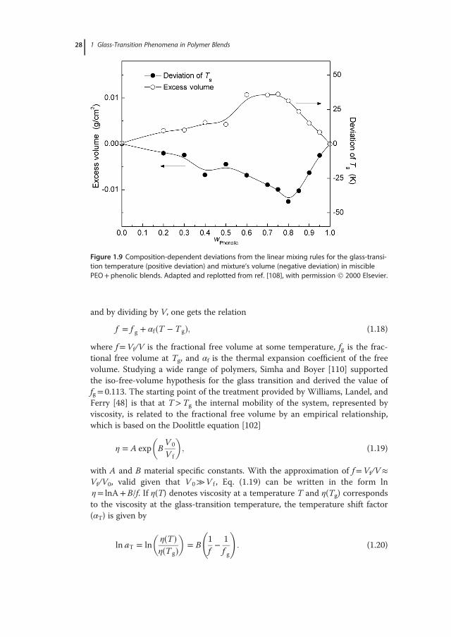
provided by free-volume theories, which consider that molecular mobility is con-trolled by the free volume, while the glass is regarded a frozen metastable state ofmatter, described by an additional kinetically controlled internal order parame-ter [78,102,103] and a P–V–T equation of state. Many different models of the glasstransition that rely on the concept of free volume [78,104] exist, including thesimple kinetic (hole) theories [66]. While not identical, these models considermolecular motions in the bulk state of polymeric materials to depend on the pres-ence of structural voids, also known as “vacancies” or “holes” of molecular size(∼0.02–0.07nm3), or imperfections in the packing order of molecules. These holesare collectively described as “free volume,” a term also used to describe the excessvolume that can be redistributed freely without energy change [78]. (It is worthnoticing, however, that the free volume available for molecular movement doesnot coincide with the total empty space in the material, which corresponds to thedifference between the geometric volume of all segments and the total volume.)The concept that local rearrangement motions in dense systems require someempty space, which can be taken by atoms involved in this motion, is intuitivelyappealing: in the liquid state, where the free volume is large, molecular movementsoccur easily and the rearrangement of chain conformations is practicallyunconstrained, while, following a decrease in temperature, the free volume shrinksuntil it is too small to allow large-scale molecular motions. As thermal expansionand viscoelastic relaxation of a solid or rubber-like material can be rationalized interms of changes in the temperature-dependent free volume, the viscoelasticbehavior of polymers and related composites has been extensively studied – withvariable success – in relation to free-volume variations [105–107]. Evidence on thesignificance of free-volume theories and support of the hypothesis that Tg isinversely proportional to free volume is often encountered in the studies of binarypolymer systems (e.g., see Figure 1.9 for miscible polyethylene oxide [PEO]+ phe-nolic blends [108]).Most theories based on the free-volume concept state that the glass transition

is characterized by an iso-free-volume fraction state, that is, they consider that“the glass transition temperature is the temperature below which the polymershave a certain universal free volume” [109]. The total volume of the material, V,obeys the relation

V � V 0 � V f ; (1.16)

where the limiting or occupied volume, V0, is associated with the hardcore orincompressible molecular volume (molecular volume at zero thermodynamictemperature or extremely high pressure) and significant volume fluctuations(from thermal motion; i.e., bond vibrations and librations). The free volume attemperatures below Tg (denoted by V ∗

f ) is considered nearly constant, andincreases only as the glass-transition temperature is exceeded. In the latter tem-perature range, free volume can be expressed as

V f � V ∗f � �T � T g� δV f

δT; (1.17)


and by dividing by V, one gets the relation

f � f g � αf �T � T g�; (1.18)

where f=Vf/V is the fractional free volume at some temperature, fg is the frac-tional free volume at Tg, and αf is the thermal expansion coefficient of the freevolume. Studying a wide range of polymers, Simha and Boyer [110] supportedthe iso-free-volume hypothesis for the glass transition and derived the value offg= 0.113. The starting point of the treatment provided by Williams, Landel, andFerry [48] is that at T>Tg the internal mobility of the system, represented byviscosity, is related to the fractional free volume by an empirical relationship,which is based on the Doolittle equation [102]

η � A exp BV 0

V f

� �; (1.19)

with A and B material specific constants. With the approximation of f=Vf/V�Vf/V0, valid given that V 0�V f , Eq. (1.19) can be written in the form lnη= lnA+B/f. If η(T) denotes viscosity at a temperature T and η(Tg) correspondsto the viscosity at the glass-transition temperature, the temperature shift factor(αT) is given by

ln aT � lnη�T �η�T g��

� B1f� 1f g

!: (1.20)

Figure 1.9 Composition-dependent deviations from the linear mixing rules for the glass-transi-tion temperature (positive deviation) and mixture’s volume (negative deviation) in misciblePEO+phenolic blends. Adapted and replotted from ref. [108], with permission 2000 Elsevier.


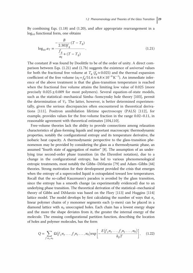
By combining Eqs. (1.18) and (1.20), and after appropriate rearrangement in alog10 functional form, one obtains

log10 aT �� B2:303f g

�T � T g�f gαf

� �T � T g�: (1.21)

The constant B was found by Doolittle to be of the order of unity. A direct com-parison between Eqs. (1.21) and (1.7b) suggests the existence of universal valuesfor both the fractional free volume at Tg (fg� 0.025) and the thermal expansioncoefficient of the free volume (αf= fg/51.6� 4.8× 10�4 K�1). An immediate infer-ence of the above treatment is that the glass-transition temperature is reachedwhen the fractional free volume attains the limiting low value of 0.025 (moreprecisely 0.025± 0.009 for most polymers). Several equation-of-state models,such as the statistical–mechanical Simha–Somcynsky hole theory [103], permitthe determination of Vf. The latter, however, is better determined experimen-tally, given the serious discrepancies often encountered in theoretical deriva-tions [111]. Positron annihilation lifetime spectroscopy (PALS) [112], forexample, provides values for the free-volume fraction in the range 0.02–0.11, inreasonable agreement with theoretical estimates [104,110].Free-volume theories lack the ability to provide connections among relaxation

characteristics of glass-forming liquids and important macroscopic thermodynamicproperties, notably the configurational entropy and its temperature derivative, theisobaric heat capacity. A thermodynamic perspective to the glass-transition phe-nomenon may be provided by considering the glass as a thermodynamic phase, anassumed “fourth state of aggregation of matter” [8]. The assumption of an under-lying true second-order phase transition (in the Ehrenfest notation), due to achange in the configurational entropy, has led to various phenomenologicalentropic treatments, most notably the Gibbs–DiMarzio [79] and Adam–Gibbs [44]theories. Strong motivation for their development provided the crisis that emergeswhen the entropy of a supercooled liquid is extrapolated toward low temperatures.Recall that the so-called Kauzmann’s paradox is avoided by the glass transition,since the entropy has a smooth change (as experimentally evidenced) due to anunderlying phase transition. The theoretical derivation of the statistical–mechanicaltheory of Gibbs and DiMarzio was based on the Flory [113] and Huggins [114]lattice model. The model develops by first calculating the number of ways that nylinear polymer chains of y monomer segments each (y-mers) can be placed in adiamond lattice with n0 unoccupied holes. Each chain has a lowest energy shapeand the more the shape deviates from it, the greater the internal energy of themolecule. The ensuing configurational partition function, describing the locationof holes and polymer molecules, has the form

Q � Xf ;ny;n0

Ω f 1ny . . . ; f iny . . . ; n0� �

exp �E f 1ny . . . ; f iny . . . ; n0� �

kβT

; (1.22)


where finy is the number of molecules packed in conformation i, E in the internalenergy of the system, and Ω is the microcanonical partition function (i.e., thetotal number of ways that the ny molecules can be packed into yny+n0 sites onthe quasi-lattice). Knowledge of the partition function allows the configurationalentropy to be determined from the relation

Sc�T � � kβT@ lnQ@T

� �V;n

� kβ lnQ; (1.23)

through which several derivations and property calculations become possible.While several of its predictions are in agreement with experimental data (e.g.,the molecular mass dependence of Tg), the validity of the theory remains ratherquestionable in the absence of rigorous mathematical justification of criticalassumptions (e.g., the actual form of the microcanonical partition function). Inan effort to reconcile thermodynamic arguments with purely dynamical aspectsof the phenomenon, it has been postulated that, although the observed glasstransitions show clear manifestations of a kinetic phenomenon, the underlyingtrue transition features equilibrium properties that are difficult to observe exper-imentally. This aspect was considered in the Gibbs–DiMarzio approach by defin-ing a new transition temperature, T2, at which the configurational entropy of thesystem reaches a critically low value Sc,0 [57] (Sc,0(T2)= 0 in ref. [79]). T2 isclearly not an experimentally measurable quantity; calculations place it approxi-mately 50° below the glass-transition temperature observed at ordinary measur-ing times. In effect, T2 is considered to be the lower limit value that Tg wouldreach in a hypothetical experiment of infinite timescale.A somewhat different phenomenological approach to an “entropy-vanishing”

glass-transition model has been presented by Adam and Gibbs [44]. The ideabehind their molecular-kinetic theory is that the liquid consists of regions thatrearrange as units, independently of their environment, when experiencing a suf-ficient fluctuation in enthalpy. Each related subsystem of the material is referredto as a cooperatively rearranging region (CRR) and has a size determined by thenumber, z, of molecules included (monomeric segments in polymers’ case). Thetemperature-dependent relaxation times for a viscous material are determinedfrom the probabilities for cooperative rearrangements to take place. A structuralrearrangement is activated with a barrier height (Δμ) proportional to the lowerlimit number z∗(T) of segments within the hypothetical critically sized CRR witha nonvanishing transition probability. The structural relaxation time is inverselyproportional to the average transition probability, providing the relation

τα�T � � τ1 expz∗ΔμkβT

� �; (1.24)

where τ1 is a constant. At high temperatures, the molecular displacements aretaken to be entirely noncollective, and the barrier height reduces to a constantArrhenius activation energy. The size of the CRR depends on temperature and isdetermined by the configurational entropy of the liquid, while an increase in thedynamic cohesive length, ξα, is anticipated with decreasing temperature. A link to


the Gibbs–DiMarzio theory is provided by the hypothesis that z∗(T) is simplyinversely proportional to the (molar) configurational entropy, z∗�T � � NAs∗c=Sc�T �,where s∗c is the configurational entropy of the critically sized CRR. By combiningthe latter equations, configurational entropy and structural relaxation time (or theshear viscosity) in the liquid state are now connected through the relation

τα�T � � τ1 expATSc

� �: (1.25)

As temperature decreases and larger units progressively form, Sc decreases untilit approaches zero at some temperature T0 (generically close to T2 and TK [54]).At this point, relaxation times and viscosity diverge, and a second-order thermo-dynamic transition is suggested to occur. The validity of Eq. (1.25) has beentested in numerous experimental studies (which, typically, use the excessentropy of the liquid over the crystal in the place of Sc) and computer simula-tions (where Sc is directly assessed) [115]. Adam and Gibbs [44] used theirentropic theory to derive a WLF-type formula for the temperature shift factor.Furthermore, considering that the configurational entropy can be calculatedfrom the relation

Sc�T � � Sc�T0� �ZTT0

ΔCp

TdT (1.26a)

and roughly assuming a hyperbolic form for the configurational part of the spe-cific heat (ΔCp∼ 1/T), it follows that

Sc�T �∝ T � T0

T; (1.26b)

from which Eq. (1.25) further derives the VFTH equation (with T0 replacing TV).One of the limitations of the Adam–Gibbs theory is that it provides no informa-tion regarding the size or number of CRRs in the system, because s∗c is not speci-fied, except as a formal lower limit that provides, in practice, no useful insight atthe microscopic level. As an extreme limit, the entropy of the smallest regioncapable of undergoing a rearrangement is obtained by the Boltzmann relation ass∗c � kβ � ln2, given that a minimum of two configurations must be available for arearrangement to take place. Adopting this value, Δμ and z∗ may be evaluatedfrom experimental data. However, the low values deduced for z∗(Tg) in a numberof glass formers suggest that the Adam–Gibbs theory, if valid, might be moreappropriate for local processes transpiring before the glass transition [13].An elaborate mean-field approach to glass formation is given by the RFOT theory

[86]. Within this framework, vitrification is described analogous to crystallization,with the difference that the system is frozen into a set of aperiodic structures insteadof a periodic crystalline structure. This theoretical ensemble ties together intelligiblyaspects of several prior concepts, notably, the unreachable thermodynamic transitionpostulated by the configurational entropy theories, the emergence of a complex free-energy landscape with numerous energy minima, and the avoided dynamical


singularity of the MCT. In this way, a low-temperature thermodynamic transition, atTK, to an ideal glass phase (accompanied by a discontinuous jump in the orderparameter, but no latent heat) is postulated to exist along with a high-temperatureergodicity breaking dynamical transition, at TMCT. These two coexisting criticalpoints are separated by a regime in which an exponentially large (in system size)number of metastable free-energy states (configurations) dominate the thermo-dynamics while trapping the dynamics. Support for the above phenomenology hasbeen found in several standard liquid models when treated within mean field-likeapproximations (see reviews by Berthier and Biroli [25], and Cavagna [116]). Thethermally activated hopping mechanisms that take control in the regime TK<T<TMCT are described in a nonperturbative way. Phenomenological arguments onlyexist [117], backed by microscopic computations [118], which describe liquid dynam-ics below the crossover at TMCT as a “mosaic state,” while a dynamical scaling theorybased on “entropic droplets” (domains of synergetic molecular motions, with linearsize ξ∗) is considered as temperature approaches TK. The entropic droplets areformed and stabilized by the competition between a favorable driving force (i.e., anincrease of the configurational entropy) and an unfavorable surface mismatch pen-alty. The mosaic length scale ξ∗, characteristic of the mosaic cells and entropic drop-lets, represents the length scale above which any consideration of metastable statesbecomes inappropriate. Assuming that thermal activation over energy barriers growswith size as (ξ∗)ψ , with ψ � θ, the super-Arrhenius τα(T) dependence is givenby [118]

lnτατ0

� �� C

YkβT

YT � Sc�T �� ψ

d�θ; (1.27)

where C is a constant, Y is a “bare” energy scale (in appropriate units), d is thedimension of space, and ψ and θ are two critical exponents. The latter are pre-dicted to obey the relation ψ � θ= 3/2, in d= 3 [117], providing an Adam–Gibbs-type formula for the relaxation time with the configurational entropy perparticle, sc(T), vanishing at the ideal glass transition TK. Several other nontrivialderivations of the RFOT, frequently based solely on phenomenological argu-ments [119], address issues such as the decoupling between translation and rota-tion, nonexponential relaxation (i.e., βKWW< 1) and its connection with fragility,the specific heat jump at the glass transition, and the accelerated segmentaldynamics close to free surfaces [120]. The reader is referred to an excellentreview by Berthier and Biroli [25] for a detailed discussion of several limitingapproximations and missing links between the pieces of this “patchwork” theory,as well as potential weaknesses of the RFOT construction in providing thedescription of finite-dimensional systems.Reference to some form of space fragmentation into dynamically and/or spa-

tially heterogeneous zones (described, for example, as “regions,” “spheres,”“domains,” or “droplets”) appears also in the frustration-limited domains (FLDs)theory. Through a series of tentative assumptions [121], this approach directlyaddresses glass formation in terms of the real space at the molecular level [92].Its critical assumptions include the existence of a locally preferred structure in a


liquid (i.e., a domain-level molecular arrangement that minimizes some localfree energy), the unfeasibility for this local structural order to expand over theentire system (i.e., the domain size is limited by frustration, or equivalently, theordered domains are deemed separated by domains of topological defects), andthe possibility to build an conjectural system in which the effect of frustrationcan be suppressed or disabled. In the context of liquids and glasses, frustrationis attributed to a competition between a short-range propensity for expansion ofa locally preferred order and global constraints that prohibit the periodic tiling ofspace with the particular local structure. Considering a system that organizesitself, at low temperatures and finite frustration level, into a mosaic of domainscorresponding to some local order, its dynamics will involve restructuring of thedomains in a thermally activated manner, using arguments similar to thoseadopted within the mosaic picture of RFOT. Under rather generic conditions,frustration produces a “narrowly avoided critical point,” that is, the orderingtransition that may possibly exist at some temperature T ∗ (above Tg) in theabsence of frustration may disappear when an infinitesimal degree of frustrationis introduced. The crossover temperature, T ∗, marks the onset of an anomaloussupermolecular (collective) behavior and it can be used to establish a scalingdescription of several collective properties of glass-forming liquids. In relation tothe existence of a pertinent heterogeneity length scale, for example, let us con-sider the free energy of a domain (of volume L3), given by

F�L;T � � c1�T �L2 � c2�T �L3 � c3�T �L5: (1.28)

The bulk free-energy gain inside the domain (second term) is modified by thestrain free energy due to frustration (last term), and this strain induces breaks inthe order that give rise to surfaces with free energy c1�L2 (first term). By mini-mizing the free energy per unit volume, F(L,T)/L3, one finds that the characteris-tic radius of the domains scales as (c1/c3)

1/3, and that their size increases whentemperature decreases without showing any divergence [121]. The presence ofstructured domains, whose size is finely tuned by the amount of frustration,readily connects to fundamental phenomena occurring in glass formers, such ascooperativity, dynamic heterogeneity, and spatial fluctuations, which directlyrationalize – at least qualitatively – nonexponential relaxation, decoupling phe-nomena, and liquid fragility. Relaxation times (and shear viscosity), for example,are predicted to exhibit a distinctive super-Arrhenius temperature dependenceat T<T ∗, of the form

τα�T � � τ1 expE1T

� ΔE�T �T

� �: (1.29)

The term ΔE(T)=BT ∗(1�T/T ∗)8/3 describes the energetic requirement forrestructuring the FLDs, and is thus assumed to be zero above T ∗, yielding a sim-ple exponential behavior. The four adjustable parameters (τ1, E1, B, T ∗) ofEq. (1.29) can be obtained by fitting of experimental data. The fragility of a glassformer is quantified by the value of parameter B, which is inversely proportionalto the degree of frustration [93]. A major weakness of this theory is the missing


identification of the locally preferred structure for molecules of nonsphericalshapes, the structural elements of most real fragile materials. It is very likely thatthe postulated formation – on supercooling – of tetrahedral or icosahedral localorder (or even of hexagonal bond orientational local order) in three-dimensionalone-component liquids with atoms interacting via spherically symmetric pairpotentials [122], has little to do with the behavior of ordinary molecular liquidsand polymers.

1.2.4.5 Percolative Phenomena in Glass FormationBoth liquids and glasses have a topologically disordered distribution of elemen-tary particles, without perceptible differences in their translation-rotation sym-metry. Their structure cannot be described in terms of repeating unit cells, asthe unit cell of any amorphous material would comprise all particles (atoms ormolecules) due to nonperiodicity. A number of approaches to the glass-transi-tion phenomenon build on alternative structure descriptions [12], such as theconsideration of the bond system rather than the set of particles. For each stateof matter, one may define a set of bonds, that is, introduce a bond lattice model,which is the congruent structure of its chemical bonds. The bond lattices ofglasses and liquids have different symmetries, in contrast to the symmetry simi-larity of particles in the liquid and glassy states of matter. Structural signatures inthe form of percolation thresholds of the Delaunay networks [123] and anincrease in icosahedral ordering near Tg [124] have been observed by computersimulations of amorphous solids and simple liquids. Interesting observationshave emerged from studies of the percolation thresholds of networks of theDelaunay simplices of different “coloring,” with each color denoting the Delau-nay sites of identical form (i.e., with identical metric properties). For example, ina molecular dynamics study of the configurations of liquid, supercooled, andquenched (glassy) rubidium, Medvedev and coworkers [123] showed that theDelaunay simplices develop macroscopic aggregates in the form of percolativeclusters. In the liquid state, low-density atomic configurations form a clusterthat goes across the whole material. This macroscopic structural organizationpermits extensive motions, like those observed in shear flow. In contrast, in theglassy state nearly tetrahedral high-density configurations contribute to the for-mation of clusters that percolate across the whole glass.The CPM explains the glass transition in terms of a percolation-type phase

transition, a percolation effect in the system of broken bonds connected with theformation of percolation clusters made of configurons [87]. A “configuron” isdefined as a fundamental configurational excitation in an amorphous materialthat involves breaking of a chemical bond and the concomitant strain-releasinglocal adjustment of centers of atomic vibration. At absolute zero temperaturebroken bonds are absent, while the concentration of thermally activated brokenbonds (configurons) is expected to increase with temperature, accompanied by aloss in material’s rigidity. Since configurons weaken the bond system, the highertheir content the lower the viscosity of the system becomes. Based on the perco-lation theory, when the concentration of configurons exceeds the threshold level,


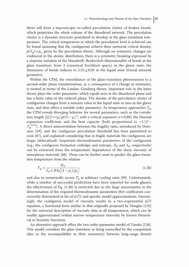
these will form a macroscopic so-called percolation cluster of broken bonds,which penetrates the whole volume of the disordered network. The percolationcluster is a dynamic structure postulated to develop at the glass-transition tem-perature. The critical temperature at which the percolation level is achieved canbe found assuming that the configurons achieve their universal critical density,p(Tg)= pc, given by the percolation theory. Although no symmetry changes areevidenced in the atomic distribution, there is a symmetry breaking expressed bya stepwise variation of the Hausdorff–Besikovitch dimensionality of bonds at theglass transition: from 3 (canonical Euclidean space), in the glassy state, thedimension of bonds reduces to 2.55± 0.05 in the liquid state (fractal networkgeometry).Within the CPM, the resemblance of the glass-transition phenomenon to a

second-order phase transformation, as a consequence of a change in symmetry,is treated in terms of the Landau–Ginsburg theory. Important role in the lattertheory plays the order parameter, which equals zero in the disordered phase andhas a finite value in the ordered phase. The density of the percolation cluster ofconfigurons changes from a nonzero value in the liquid state to zero in the glassystate, and thus offers a suitable order parameter. As temperature approaches Tg,the CPM reveals diverging behavior for several parameters, such as the correla-tion length [ξ(T)= ξ0/|p(T)� pc|

n, with a critical exponent n= 0.88], the thermalexpansion coefficient, and the heat capacity (both proportional to ∼1/|T�Tg|

0.59). A direct anticorrelation between the fragility ratio, introduced by Dore-mus [59], and the configuron percolation threshold has been postulated toexist [87], and explained considering that in fragile materials the configurons arelarger (delocalized). Important thermodynamic parameters of the configurons(e.g., the configuron formation enthalpy and entropy, Hd and Sd, respectively)can be extracted from the temperature dependence of the shear viscosity ofamorphous materials [88]. These can be further used to predict the glass-transi-tion temperature from the relation

T g � Hd

Sd � R ln �1 � pc�=pc� � (1.30)

and also to numerically access Tg at arbitrary cooling rates [89]. Unfortunately,while a number of successful predictions have been reported for oxide glasses,the effectiveness of Eq. (1.30) is restricted due to the large uncertainties in thedetermination of the required thermodynamic parameters (five coefficients con-currently determined in fits of η(T)) and specific model approximations. Interest-ingly, the configuron model of viscosity results in a two-exponential η(T)equation, a functional form similar to that originally proposed by Douglas [125]for the universal description of viscosity data at all temperatures, which can bereadily approximated (within narrow temperature intervals) by known theoreti-cal or heuristic functions.An alternative approach offers the two-order-parameter model of Tanaka [126].

This model considers the glass transition as being controlled by the competition(due to the incompatibility in their symmetry) between long-range density


ordering toward crystallization and short-range bond ordering toward the forma-tion of long-lived rigid structural elements (designated as “locally favored struc-tures”). The supercooled liquid is described as a frustrated metastable liquid stateconsisting of metastable solid-like islands, in a sea of short-lived random normal-liquid structures, which exchange each other dynamically at the rate of the struc-tural relaxation time. Depending on the type of measurement, Tg can be definedeither as the temperature at which the average lifetime of the metastable islandsexceeds the characteristic observation time or as the temperature where percola-tion of long-lived metastable islands occurs. The average fraction of locallyfavored structures is regarded as a suitable measure of fragility (with a higherfraction indicating a stronger liquid), while extensive reasoning addresses thecrossover from the noncooperative to the cooperative regime and the origin ofthe non-Arrhenius behavior of the structural relaxation.At present, approaches like those mentioned above simply provide an interest-

ing, yet incomplete, picture of glass formation, given the fact that they canaddress only a narrow range of its plethoric phenomenology.

1.3Manipulating the Glass Transition

The glass-transition temperature reflects the ease by which polymer chains com-mence waggling and break out of the rigid glassy state into the soft rubbery statein the course of heating. Its location is thus primarily regulated by intrinsic charac-teristics of the macromolecular system (Section 1.3.1), typically related to thechemical structure (main-chain structure, tacticity, type of pendant groups, etc.),chain conformations, and the degree of polymerization (molecular mass). Knowl-edge of the potential influence of each of these factors is a prerequisite – butclearly not the only – for appropriate selection of the components in binary andternary mixtures and the preparation of polymer composites with finely adjustedproperties and structural characteristics. Besides blending, which is comprehen-sively treated later in this chapter, reference should also be made to a number oftechnologically important externally controllable processes (application of pressure,orientation processes, presence of additives, electron-beam irradiation, etc.), chemi-cal reactions (copolymerization, curing), or physical phenomena (aging, crystalliza-tion), with a substantial bearing on the glass structure and the temporal response(during storage or service life) of engineering polymeric materials (Section 1.3.2).Guidance for targeted polymeric molecular design may come from explicit

theoretical and simulation methodologies that aim to predict material’s propert-ies from its molecular details. Freed and coworkers [127], for example, developeda generalized entropy theory that combines the lattice cluster theory – for asemiflexible-chain polymer fluid – with the Adam–Gibbs model for the struc-tural relaxation time. Their model provided a rational, predictive framework forcalculating the essential properties (including Tg and fragility) of glass-formingfluids as a function of their molecular architecture, bond stiffness, cohesive


interaction energy, pressure, molar mass, concentration and structure of addi-tives, and so forth. The estimates appear to corroborate several of the experi-mentally established general trends discussed below. Simulation approaches, onthe other hand, usually employ either quantitative structure–property relation-ship (QSPR) models (where structural and quantum-chemical descriptors of per-ceived significance along with group additive methods are typically used inrelevant estimations [128,129]) or atomistic modeling techniques (where fullatomic detail of the polymers is considered, as in molecular dynamics simula-tions [130]). For selected polymers, interesting information on various struc-ture–property dependences, such as the variation of Tg with chain stiffness andsubstituent volume [131] or the type of the polymerization initiator [132], hasbeen derived from QSPR studies.

1.3.1

Effects of Chemical Structure

The location of the glass transformation range is representative of the flexibilityof polymer chains, which in turn is determined by the degree of freedom withwhich their segments rotate along the backbone. As a result, low Tgs are typicalof linear polymers with single covalent bonds and a high degree of rotationalfreedom about σ bonds in the main chain, while stiffening groups along the back-bone (e.g., aromatics and cyclic structures) reduce chain flexibility and increaseintermolecular cohesive forces. For instance, the incorporation of a p-phenylenering (Ph) into polyethylene’s (PE) monomeric unit gives poly(p-xylylene)[(��CH2��Ph��CH2��)n], with a glass-transition temperature (�+80 °C) signifi-cantly elevated compared to that observed in various commercial PEs (�130 °Cto �80 °C). Tacticity has considerable bearing on the rotational energy require-ments of the backbone. In the case of mono- and disubstituted vinyl polymers,(��CH2��CXY��)n, for example, Karasz and MacKnight [133] indicate that stericconfiguration affects Tg only when the substitutes are different, and neither ofthem is hydrogen. Based on the Gibbs–DiMarzio theory of the glass transition,the increase observed going from isotactic and highly syndiotactic polymers canbe related to the larger difference among the energy levels between rotationalisomers in syndiotactic chains. In monosubstituted vinyl polymers, where theother substitute is hydrogen, the energy differences between the rotational statesof the two pairs of isomers are comparable and the effect of tacticity is weak (e.g.,polystyrene[PS] and poly(vinyl acrylate)s; Table 1.1). If the different tactic config-urations of a single disubstituted vinyl polymer are considered, the glass-transi-tion temperature appears to increase with the increasing content of syndiotactictriads. This trend is clearly demonstrated by poly(N-vinyl carbazole) (PVK) (i.e.,Tg= 126 °C, 227 °C, and 276 °C, for isotactc (i-), atactic (a-), and syndiotactic (s-)PVK, respectively) [134]), poly(methyl methacrylate) (PMMA) [16,135], and sev-eral other poly(vinyl methacrylate)s (Table 1.1).The chemical nature (e.g., polarity and ionicity), bulkiness, and flexibility of the

groups attached to a polymer chain are often used to adjust its glass-transition

1.3 Manipulating the Glass Transition 37

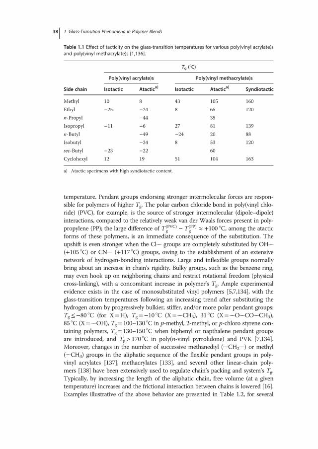
temperature. Pendant groups endorsing stronger intermolecular forces are respon-sible for polymers of higher Tg. The polar carbon chloride bond in poly(vinyl chlo-ride) (PVC), for example, is the source of stronger intermolecular (dipole–dipole)interactions, compared to the relatively weak van der Waals forces present in poly-propylene (PP); the large difference of T �PVC�

g � T �PP�g � �100 °C, among the atactic

forms of these polymers, is an immediate consequence of the substitution. Theupshift is even stronger when the Cl�� groups are completely substituted by OH��(+105 °C) or CN�� (+117 °C) groups, owing to the establishment of an extensivenetwork of hydrogen-bonding interactions. Large and inflexible groups normallybring about an increase in chain’s rigidity. Bulky groups, such as the benzene ring,may even hook up on neighboring chains and restrict rotational freedom (physicalcross-linking), with a concomitant increase in polymer’s Tg. Ample experimentalevidence exists in the case of monosubstituted vinyl polymers [5,7,134], with theglass-transition temperatures following an increasing trend after substituting thehydrogen atom by progressively bulkier, stiffer, and/or more polar pendant groups:Tg��80 °C (for X=H), Tg=�10 °C (X=��CH3), 31 °C (X=��O��CO��CH3),85 °C (X=��OH), Tg= 100–130 °C in p-methyl, 2-methyl, or p-chloro styrene con-taining polymers, Tg= 130–150 °C when biphenyl or napthalene pendant groupsare introduced, and Tg> 170 °C in poly(n-vinyl pyrrolidone) and PVK [7,134].Moreover, changes in the number of successive methanediyl (��CH2��) or methyl(��CH3) groups in the aliphatic sequence of the flexible pendant groups in poly-vinyl acrylates [137], methacrylates [133], and several other linear-chain poly-mers [138] have been extensively used to regulate chain’s packing and system’s Tg.Typically, by increasing the length of the aliphatic chain, free volume (at a giventemperature) increases and the frictional interaction between chains is lowered [16].Examples illustrative of the above behavior are presented in Table 1.2, for several

Table 1.1 Effect of tacticity on the glass-transition temperatures for various poly(vinyl acrylate)sand poly(vinyl methacrylate)s [1,136].

Tg (°C)

Poly(vinyl acrylate)s Poly(vinyl methacrylate)s

Side chain Isotactic Atactica) Isotactic Atactica) Syndiotactic

Methyl 10 8 43 105 160

Ethyl �25 �24 8 65 120

n-Propyl �44 35

Isopropyl �11 �6 27 81 139

n-Butyl �49 �24 20 88

Isobutyl �24 8 53 120

sec-Butyl �23 �22 60

Cyclohexyl 12 19 51 104 163

a) Atactic specimens with high syndiotactic content.


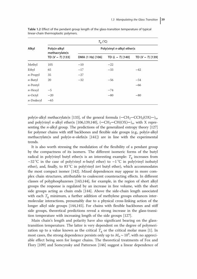
poly(n-alkyl methacrylate)s [133], of the general formula (��CH2��CCH3(OX)��)n,and poly(vinyl n-alkyl ether)s [106,139,140], (��CH2��CH(OX)��)n, with X repre-senting the n-alkyl group. The predictions of the generalized entropy theory [127]for polymer chains with stiff backbones and flexible side groups (e.g., poly(n-alkylmethacrylate)s and poly(n-α-olefin)s [141]) are in line with the experimentaltrends.It is also worth stressing the modulation of the flexibility of a pendant group

by the compactness of its isomers. The different isomeric forms of the butylradical in poly(vinyl butyl ether)s is an interesting example: Tg increases from�32 °C in the case of poly(vinyl n-butyl ether) to �1 °C in poly(vinyl isobutylether), and, finally, to 83 °C in poly(vinyl tert butyl ether), which accommodatesthe most compact isomer [142]. Mixed dependences may appear in more com-plex chain structures, attributable to coalescent counteracting effects. In differentclasses of polyphosphazenes [143,144], for example, in the region of short alkylgroups the response is regulated by an increase in free volume, with the shortside groups acting as chain ends [144]. Above the side-chain length associatedwith each Tg minimum, a further addition of methylene groups enhances inter-molecular interactions, presumably due to a physical cross-linking action of thelonger alkyl side groups [144,145]. For chains with flexible backbones and stiffside groups, theoretical predictions reveal a strong increase in the glass-transi-tion temperature with increasing length of the side groups [127].Main chain’s length and polarity have also significant bearing on the glass-

transition temperature. The latter is very dependent on the degree of polymeri-zation up to a value known as the critical Tg or the critical molar mass [1]. Inmost cases, the strong dependence persists only up to Mn∼ 104, with no appreci-able effect being seen for longer chains. The theoretical treatments of Fox andFlory [109] and Somcynsky and Patterson [146] suggest a linear dependence of

Table 1.2 Effect of the pendant group length of the glass-transition temperature of typicallinear-chain thermoplastic polymers.

Tg (°C)

Alkyl Poly(n-alkylmethacrylate)s

Poly(vinyl n-alkyl ether)s

TD (V − T) [133] DMA (1 Hz) [106] TD (L − T) [140] TD (V − T) [139]

Methyl 105 �10 �22Ethyl 65 �17 �33 �42n-Propyl 35 �27n-Butyl 20 �32 �56 �54n-Pentyl �66n-Hexyl �5 �74n-Octyl �20 �80 �80n-Dodecyl �65


Tg on the inverse molar mass of a homopolymer, expressed as

T g � T1g � K

Mn: (1.31)

In this relation, K is a constant depending on the polymer, Mn is the number-aver-aged molecular mass of the homopolymer, and T1

g is the glass-transition tempera-ture of a linear chain of “infinite” length. For PVC, for example, Pezzin andcoworkers [147] reported values of T1

g � 78 °C and K= 8.05× 104 (for 3× 103�Mn� 105). Equation (1.31) can be deduced from the free-volume theory, takinginto account that terminal (end) groups bring about more free volume than theinternal ones [148]. More satisfactory description of the experimental pattern hasbeen reported using functional forms deriving from the statistical–mechanicalGibbs–DiMarzio [80] theory. For commercial polymers, the influence of Mn varia-tion on Tg is insignificant and is almost always overtaken by other factors. Notealso that a decrease in chain’s flexibility frequently stems from an increase in thedensity and/or the strength of interchain interactions. The first effect is illustratedin the gradual change of the glass-transition temperature of PE from �7 °C to137 °C, with chlorination levels increasing from 28.2% to 77.4% [149].

1.3.2

Externally Controlled Processes or Treatments

1.3.2.1 Pressure EffectsThe measurement of changes in the glass-transition temperature with pressure var-iations has become an important topic of polymer science, and new experimentalstudies and theoretical interpretations of pressure effects are in development [150].In practical terms, interest is primarily directed toward the studies of product fail-ure at high-pressure applications, while polymer engineering seeks information onthe pressure dependence of the glass transition of polymers – in part – as a resultof its involvement in the commercial large-scale production or treatment of poly-mer mixtures (e.g., in hot-melt extrusion and compression molding). In general, Tg

in polymers increases with increasing pressure (Figure 1.10 [150,151]), as expectedfrom the generalized Ehrenfest relations applied to the glass–liquid transforma-tion [152] and in accordance with predictions of free-volume theories of the glasstransition [1]. The change is roughly described by the relation deriving if one con-siders the continuity of volume at the transition,

@T g

@P

� �T

� ΔκTΔα

; (1.32)

while a much better description of a wider collection of experimental data [153]is provided by the second Ehrenfest relation, which considers continuity ofentropy at the transition,

@T g

@P

� �T

� VTΔαΔCp

: (1.33)


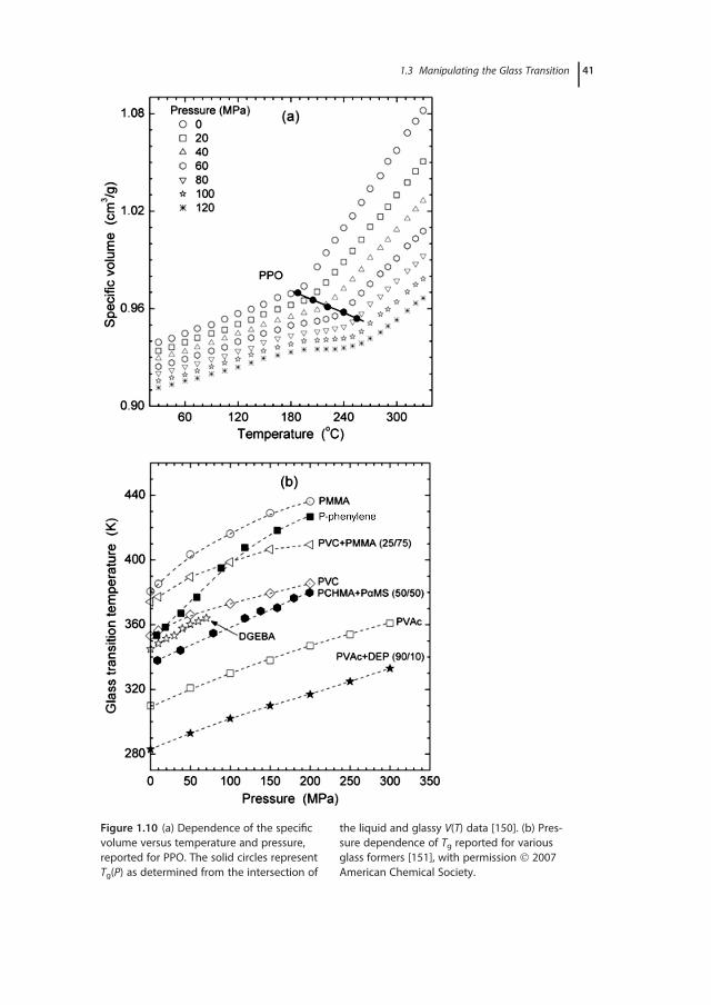
Figure 1.10 (a) Dependence of the specificvolume versus temperature and pressure,reported for PPO. The solid circles representTg(P) as determined from the intersection of

the liquid and glassy V(T) data [150]. (b) Pres-sure dependence of Tg reported for variousglass formers [151], with permission 2007American Chemical Society.


The latter relation has been recently shown by Schmelzer [19] to be derived usingan entropy-based approach for viscous flow and relaxation (Adam–Gibbs model).For all glass formers, the change in Tg with pressure is linear at low pressures, butthe pressure coefficient of the glass-transition temperature decreases with increas-ing pressure. The empirical relation proposed by Andersson and Andersson [154]

T g � k1 1 � k2k3P

� �1=k2

(1.34)

with k1, k2, and k3 material constants, is frequently used to describe experimentaldata. A rough estimate considers an increase of the glass-transition temperatureat a rate of around 20°–25° per kbar of pressure [1]. In view of that, the stiffeningeffect of pressure (vitrification) becomes important only in the case of applica-tions at very high pressures, as well as in engineering operations where thepolymer is processed near Tg.

1.3.2.2 Crystallization EffectsPolymers with a high tendency for crystallization are anticipated if their molecu-lar geometry permits the formation of specific molecular orientations. As theglass-transition phenomenon activates only in the amorphous regions of a par-tially crystalline material, the intensity of the signal is controlled by both thedegree of crystallinity and the formation of a “rigid amorphous fraction”(RAF) [155,156]. The latter term is often used to distinguish strongly hindered(often presumed immobile) chains at the amorphous–crystalline interface frommobile chains in the remaining amorphous phase (the “mobile amorphous frac-tion” (MAF); see also Section 1.7.2). As a consequence of the need to accommo-date flexible molecules of typically 1–100 μm length into micro- or nano-sizedintercrystallite regions, a crossing of the interface by the long molecules is rathercommon. This produces a strong coupling between crystalline and amorphousphases and a dependence of molecular mobility on segment’s proximity to crys-tallite surfaces. Because of that, the main glass-transition signal in semicrystallinepolymers is broader than that of the amorphous ones and extends toward thehigh-temperature side [27]. Surprisingly, the transition temperature may eitherincrease [5] or decrease with increasing degree of crystallinity. In poly(ethyleneterephthalate) (PET), for example, the amorphous specimen Tg of 65 °C changesto 92 °C in a highly crystalline material (relaxational DSC data [157]), while, inthe case of poly(4-methyl-1-pentene), an increase in crystallinity from 0% to 76%is accompanied by a drop in Tg from 29 °C to 18 °C (specific volume versustemperature thermomechanical data [158]). A broadly accepted explanation forthese opposite shifts is still missing. A plausible explanation, however, considersthe difference in the relative densities of the amorphous and crystalline phases asthe determining factor [7]. In many polymers, the coupling observed at the inter-face also causes a separate glass transition for the RAF. This portion of the polymermay lose its rigid character below the melting temperature of the surroundingcrystals, within the melting region, or even above the melting temperature [156].


When a molten polymer is subjected to stretch during processing, orientationof the chains occurs accompanied by a significant rise of its glass-transition tem-perature. Highly oriented materials, such as films or fibers, can yield an apparentTg, that is, by as much as 30° higher than that of the unoriented amorphousmaterial [159,160]. Even stronger dependences are observed when orientationcoexists with, or promotes, crystallization [159]. A common interpretation ofthese changes is based on the decrease of the free volume with increasing orien-tation, as chains in the amorphous phase are constrained in relatively close-packed elongated forms.

1.3.2.3 Plasticizer EffectsIn order to improve the flexibility, processability, and utility of a given poly-mer, it is often necessary to decrease its glass-transition temperature. Thiscan be accomplished by the addition of low-molecular-mass chemical com-pounds (“diluents”), mostly nonvolatile and chemically inert liquids, referredto as plasticizers [161]. A plasticizer may be considered as a substance,breaking intermolecular bonds in a polymer network, or even as a lubricant,reducing intermolecular friction and by this increasing deformability of thestructure [162]. The ensuing reduction of the cohesive forces between neigh-boring polymer chains facilitates molecular rotations with a concomitantdecrease in Tg. From the perspective of free-volume theories, plasticizer mol-ecules may be considered to increase free volume by pushing apart neighbor-ing chains, permitting the translational and rotational mobility of theirsegments to be retained to temperatures lower than those in the pure poly-mer. In contrast to molecular plasticizers that decrease the stiffness of theglassy polymer (lowering modulus and tensile strength, followed by anincrease in elongation), some chemical compounds act as antiplasticizers,increasing the material’s stiffness while they produce a (softer) depression ofTg. The addition of an antiplasticizer has been determined by Riggleman andcoworkers [163] to cause significant changes in the long-wavelength propert-ies, which are associated with an enhanced packing efficiency in the glassstate (e.g., a decrease in κT) and increased material stiffness (i.e., an increasein shear modulus, bulk modulus, and Poisson ratio). The efficiency of anypotential plasticizer/antiplasticizer is expected to depend on its polarity, solu-bility parameter, stiffness, density, and loading (weight, volume, or molarfraction). These factors manipulate the relative importance of the enthalpicand entropic contributions to the glass-transition temperature. An analysis ofthe issue, based again on the generalized entropy theory, exemplifies the sig-nificance of diluent’s molecular properties [141]: plasticization is favored bysmall additives whose cohesive energies are less than the cohesive energy ofthe host polymer (i.e., only weak attractive interactions between the diluentand the polymer matrix are present), while antiplasticization is promoted inthe opposite case. Absorbed water often functions as a plasticizer on manyhydrophilic materials (e.g., polyamides, starches, and sugars), while the simul-taneous occurrence of plasticization and antiplasticization effects (yet in


different concentration ranges) is not uncommon in hydrated amorphousfood matrices [164]. Weakly polar esters are good plasticizers because theytend to be miscible with many polar and nonpolar polymers. The most com-monly used plasticizers are obtained from phthalic acid and include diethyl,dibutyl, and n-dioctyl phthalates. Smaller and/or more flexible diluents gen-erally depress Tg more than the larger ones. In terms of application, however,low-molecular-mass plasticizers present some disadvantages, caused by theirvolatility and tendency for diffusion within the final product (and subsequentleaching), potentially posing environmental dangers. This fact has provokedthe development of polymeric plasticizers, formed by polymers of low Tg andmiscible with the base polymer [2], which provide materials with longer ser-vice times. A typical example is PVC plasticized with acrylonitrile butadienerubber or copolymers of ethylene vinyl acetate [165].

1.3.2.4 Filler EffectsSeveral properties, such as the thermal stability, mechanical strength, or elec-trical conductivity of a polymeric material, can also be regulated by incorpo-rating microscopic or nanoscopic inorganic fillers. Particulate systemstypically involve polymers with finely dispersed clays, alumina, silica, silver orgold nanoparticles, carbon blacks, carbon nanofibers, and single-wall or mul-tiwall carbon nanotubes [166]. The level of adjustment in the properties ofthe host matrix is determined by a number of factors, including the nature,size, amount (load), and surface chemistry of the filler, as well as the level ofinteraction between the components. In a number of studies [166,167], aloosened molecular packing of the polymer chains in the presence of thenanoparticles results in enhanced molecular mobility and a lower Tg for thecomposite. In contrast, wetted nanoparticle interfaces experiencing strongattractive interactions (as a rule, hydrogen bonding) with the polymer bringabout moderate-to-strong upshifts in the glass-transition temperature [168].The presence of a rigid amorphous polymer fraction around the nanopar-ticles has been well documented [39,169,170]. Calorimetric and dielectricresults from different filler–polymer combinations suggest that the constraintin segmental mobilities does not extend throughout the material but affectsonly an interfacial layer with a thickness of a few nanometers. In some cases,this interfacial layer has been identified as totally immobilized [169], while inothers, an additional glass transition emerges as a separate signal at highertemperature, or as shoulder at the high-temperature flank of the relaxationpeak (e.g., in poly(dimethyl siloxane)+ SiO2 nanocomposites [171]). Interpar-ticle spacing efficiently modulates the apparent glass-transition temperatureof the nanocomposite [172–174], with different shifts recorded even in thesame particulate system depending on the state of dispersion. This is clearlyillustrated in the current thermograms of natural rubber–silica nanocompo-sites (Figure 1.11), where finely dispersed silica produces a small systematicincrease of Tg compared to the neat rubber, while no change or a marginaldecrease is observed for aggregated silica nanoparticles [175].


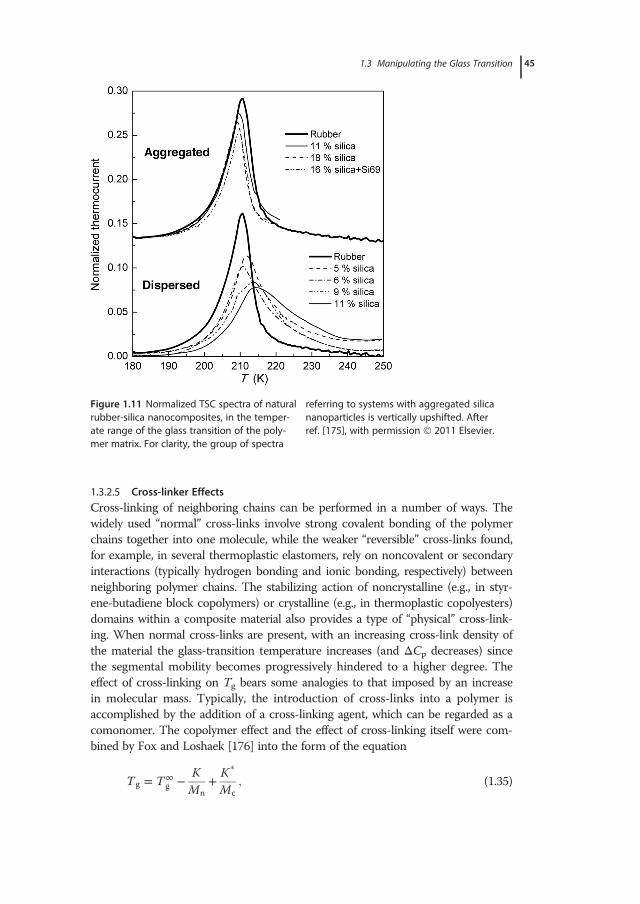
1.3.2.5 Cross-linker EffectsCross-linking of neighboring chains can be performed in a number of ways. Thewidely used “normal” cross-links involve strong covalent bonding of the polymerchains together into one molecule, while the weaker “reversible” cross-links found,for example, in several thermoplastic elastomers, rely on noncovalent or secondaryinteractions (typically hydrogen bonding and ionic bonding, respectively) betweenneighboring polymer chains. The stabilizing action of noncrystalline (e.g., in styr-ene-butadiene block copolymers) or crystalline (e.g., in thermoplastic copolyesters)domains within a composite material also provides a type of “physical” cross-link-ing. When normal cross-links are present, with an increasing cross-link density ofthe material the glass-transition temperature increases (and ΔCp decreases) sincethe segmental mobility becomes progressively hindered to a higher degree. Theeffect of cross-linking on Tg bears some analogies to that imposed by an increasein molecular mass. Typically, the introduction of cross-links into a polymer isaccomplished by the addition of a cross-linking agent, which can be regarded as acomonomer. The copolymer effect and the effect of cross-linking itself were com-bined by Fox and Loshaek [176] into the form of the equation

T g � T1g � K

Mn� K�Mc

; (1.35)

Figure 1.11 Normalized TSC spectra of naturalrubber-silica nanocomposites, in the temper-ate range of the glass transition of the poly-mer matrix. For clarity, the group of spectra

referring to systems with aggregated silicananoparticles is vertically upshifted. Afterref. [175], with permission 2011 Elsevier.


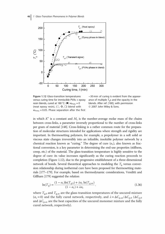
in which K∗ is a constant and Mc is the number-average molar mass of the chainsbetween cross-links, a parameter inversely proportional to the number of cross-linksper gram of material [148]. Cross-linking is a rather common route for the prepara-tion of molecular structures intended for applications where strength and rigidity areimportant. In thermosetting polymers, for example, a prepolymer in a soft solid orviscous state changes irreversibly into an infusible, insoluble polymer network by achemical reaction known as “curing.” The degree of cure (αc), also known as frac-tional conversion, is a key parameter in determining the end-use properties (stiffness,creep, etc.) of the material. The glass-transition temperature is highly sensitive to thedegree of cure: its value increases significantly as the curing reaction proceeds tocompletion (Figure 1.12), due to the progressive establishment of a three-dimensionalnetwork of bonds. Several theoretical approaches to modeling the Tg versus conver-sion relationship during isothermal cure have been proposed for thermosetting mate-rials [177–179]. For example, based on thermodynamic considerations, Venditti andGillham [179] suggested the relation

ln�T g� � �1 � αc�ln�T g;0� � λαc ln�T g;1��1 � αc� � λαc

; (1.36)

where Tg,0 and Tg,1 are the glass-transition temperatures of the uncured mixture(αc= 0) and the fully cured network, respectively, and λ=ΔCp,1/ΔCp,0 (ΔCp,0

and ΔCp,1 are the heat capacities of the uncured monomer mixture and the fullycured network, respectively).

Figure 1.12 Glass-transition temperaturesversus curing time for immiscible PVAc+ epoxyresin blends, cured at 180 °C: (•) wPVAc= 0(neat epoxy resin), (○, ⋄, □) blend withwPVAc= 0.05. Phase separation after the first

∼30min of curing is evident from the appear-ance of multiple Tgs and the opacity in theblends. After ref. [180], with permission 2007 John Wiley & Sons.


1.3.2.6 Geometric Confinement EffectsParallel to sophisticated model simulations, the glass-transition dynamics andthe characteristic transition temperature of nanoscopically confined glass-form-ing materials have been intensively studied with the purpose of elucidating thecharacteristic length scale of cooperativity experimentally [181]. A strong bodyof scientific literature [182] has been accumulated for a number of systems,including – but not limited to – amorphous layers confined between neighbor-ing crystal lamellae [181], polymers in clay galleries, intercalated or exfoliatedclay-polymer hybrid systems [183], colloidal systems, micro/nanoemulsions,ultrathin films, multilayers, organic glass formers within controlled poreinorganic glasses, as well as binary systems (e.g., filler+ polymer, diluent+polymer, and binary polymer blends [184–186]) and copolymers [187]. Of par-ticular merit appear to be studies on the behavior of organic liquids and poly-mers confined in nanopores and of polymers in the form of thin films, for whichstriking changes are often recorded for confining dimensions below 10 nm inporous environments, and for even higher thicknesses in free-standing polymerfilm geometries [181,188,189]. Excellent reviews on the topic [181,182,189,190]clearly demonstrate that we are far from having achieved a final, complete, andself-consistent, picture for the behavior of glass-forming materials in confinedstates. Confinement-induced perturbations of the molecular relaxation dynamicsand the apparent glass-transition signal, usually quantified by the shift ofthe transition temperature �ΔT∗

g � T conf :g � Tbulk

g � and changes in the relativestrength and breadth of the respective transitions, clearly demonstrateremarkable, irregular, and often contradictory dependences on the surfacechemistry of the confining system (i.e., the interfacial energy controlled bythe nature of the repulsive/soft or attractive/rough surfaces), compositional,and structural characteristics of the confined phase (e.g., polarity, molecularmass, chain conformation/stereoregularity, steric hindrance, and fragility),and the topology (fractality, porosity) or degree of confinement [182,189,190].Attempts to unify interpretations and resolve pending questions stumble onthe diversity of features which real systems demonstrate (depending, amongother parameters, on the type and strength of interactions between the com-ponents), and to a lower degree on conflicting results that arise from intrin-sic differences between the experimental techniques employed (e.g., widevariations in sensitivity and length scale of the probe) or even subtle varia-tions in thermal histories and sample pretreatments [182]. A matter ofintense research debate, consonant with the intriguing nature of the glass-transition phenomenon and the diversity of factors controlling it, constitutesreports of different trends in the variation of the transition temperature�ΔT∗

g� with changes in the confining length obtained using different experi-mental techniques for nearly identical systems [189,191]. Inconclusive argu-ments also appear with respect to the potential influence of the molar massof the confined polymer on the type and strength of the ΔT∗

g variation [189].Since Jackson and McKenna [192] first observed the depression of the glass-

transition temperature of organic liquids (of ortho-terphenyl and benzyl alcohol)


into the pores of a controlled pore glass, a number of studies on hydrogenbonded glass formers have demonstrated the glass-transition temperature todecrease [189,190], remain unchanged, or even increase with increasing confine-ment. This complex behavior is in part related to the interplay among surfaceeffects (e.g., strong hydrogen-bonding interactions between the confined mole-cules and the natural (uncoated) pores) and the intrinsic or confinement effect(e.g., breakdown of the cooperative motion, which translates into a change in thecooperativity length scale). Hydrogen-bonded liquids confined in silanized nano-pores generally display accelerated relaxation dynamics, a broadening of therelaxation function, and lower glass-transition temperatures compared to thoserecorded in the bulk or when confined in unsilanized pores. Matrices with hydro-philic (hard) surfaces have been found to produce diverse responses, beyond theabovementioned rather typical trend. Examples provide the bulk-like behaviorobserved for salol in unsilanized MCM-41 nanoporous glass [193], and the eleva-tion of the glass-transition temperature – in selected confining dimensions only –of glycerol, ethylene glycol, and oligomeric propylene glycol in unsilanized nano-porous glasses [193,194].The majority of published results on thin polymer films suggest that the dynam-

ics of thin polymer layers with free surfaces (free-standing films) or in contact withrepulsive/soft surfaces (softly supported films) are governed by entropic effects,including chain-end segregation, density anomalies, and disentanglement. The dif-ferent energetic states of the molecules located on the free surface and in the inter-nal (bulk) regions of any material, and in particular the existence of an enhancedmobility layer at the free surface of polymers, remain a subject of intensedebate [195]. The diversity of results obtained in several investigations of ultrathinor multilayer films, binary polymer blends [186], and other systems is compoundedby the fact that different length scales (or extends of cooperativity) are impacted byconfinement differently [196]. Several results support the idea of Keddie et al. [197]that a sufficiently thin liquid-like layer adjacent to the free surface exists, withreduced Tg due to the reduced requirements for cooperative segmental mobility.de Gennes [198] has further suggested a “sliding-motions” mechanism for propa-gating the mobility of the near-surface segments to depths comparable to the over-all size of the polymer molecules. The perturbations caused by the surface layer arethus allowed to propagate some tens of nanometers into the film interior, usuallyresulting in a strong reduction in Tg with decreasing film thickness (D). This varia-tion can be described by the relation

T g�D� � D�2k � D��ξ � D�2 T g�1�; (1.37)

where Tg(1) denotes the thickness-independent value determined in sufficientlythick samples, and k and ξ are model-specific constants [199]. For 2k= ξ, Eq.(1.37) reduces to a Michaelis–Menten-type function [Tg(D)=Tg(1)/(1+ ξ/D)],which provides a satisfactory description of several experimental dependences. Incontrast, strong enthalpic forces in the vicinity of the polymer–substrate interface(e.g., hydrogen bonds between films of PMMA, poly(2-vinyl pyridine) [P2VP], or


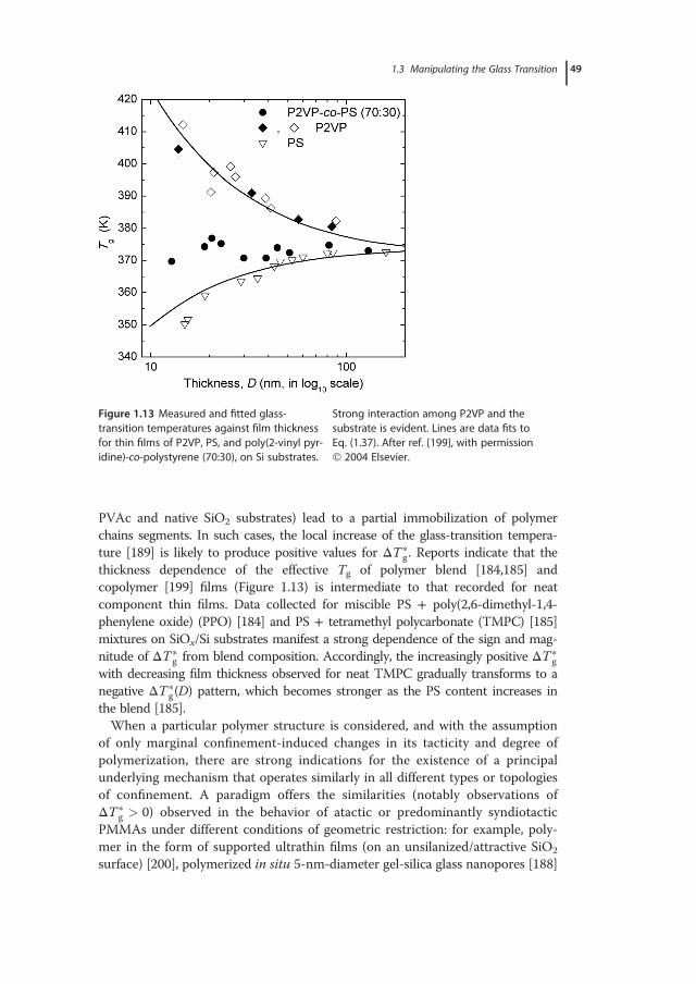
PVAc and native SiO2 substrates) lead to a partial immobilization of polymerchains segments. In such cases, the local increase of the glass-transition tempera-ture [189] is likely to produce positive values for ΔT∗

g. Reports indicate that thethickness dependence of the effective Tg of polymer blend [184,185] andcopolymer [199] films (Figure 1.13) is intermediate to that recorded for neatcomponent thin films. Data collected for miscible PS + poly(2,6-dimethyl-1,4-phenylene oxide) (PPO) [184] and PS + tetramethyl polycarbonate (TMPC) [185]mixtures on SiOx/Si substrates manifest a strong dependence of the sign and mag-nitude of ΔT∗

g from blend composition. Accordingly, the increasingly positive ΔT∗g

with decreasing film thickness observed for neat TMPC gradually transforms to anegative ΔT∗

g(D) pattern, which becomes stronger as the PS content increases inthe blend [185].When a particular polymer structure is considered, and with the assumption

of only marginal confinement-induced changes in its tacticity and degree ofpolymerization, there are strong indications for the existence of a principalunderlying mechanism that operates similarly in all different types or topologiesof confinement. A paradigm offers the similarities (notably observations ofΔT∗

g > 0) observed in the behavior of atactic or predominantly syndiotacticPMMAs under different conditions of geometric restriction: for example, poly-mer in the form of supported ultrathin films (on an unsilanized/attractive SiO2

surface) [200], polymerized in situ 5-nm-diameter gel-silica glass nanopores [188]

Figure 1.13 Measured and fitted glass-transition temperatures against film thicknessfor thin films of P2VP, PS, and poly(2-vinyl pyr-idine)-co-polystyrene (70:30), on Si substrates.

Strong interaction among P2VP and thesubstrate is evident. Lines are data fits toEq. (1.37). After ref. [199], with permission 2004 Elsevier.


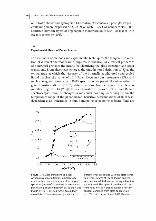
or in hydrophobic and hydrophilic 13-nm-diameter controlled pore glasses [201],containing finely dispersed SiO2 [202] or metal (Ce, Co) nanoparticles [203],restricted between layers of organophilic montmorillonite [204], or loaded withorganic bentonite [205].

1.4Experimental Means of Determination

For a number of methods and experimental techniques, the temperature varia-tion of different thermodynamic, physical, mechanical, or electrical propertiesof a material provides the means for identifying the glass transition and othertransitions. From rheometry emerges the time-honored definition of Tg as thetemperature at which the viscosity of the internally equilibrated supercooledliquid reaches the value of 1012 Pa s. Electron spin resonance (ESR) andnuclear magnetic resonance (NMR) spectroscopies permit the observation ofglass transformations and Tg determinations from changes in molecularmobility (Figure 1.14 [206]). Fourier transform infrared (FTIR) and Ramanspectroscopies monitor changes in molecular bonding, occurring within thetemperature range of the phenomenon. Sensitive determinations of thickness-dependent glass transitions in thin homopolymer or polymer blend films are

Figure 1.14 Glass transitions and ESR:Arrhenius plots of nitroxide radical (probe)rotational correlation times and loss tangentspectrum (inset) of an immiscible semi-inter-penetrating polymer network based on PI andPMMA (w1/w2= 1; 4% dicumyl peroxide, PIcross-linker). Three crossover points, the

extreme ones associated with the glass transi-tion temperatures of PI and PMMA and theintermediate related to a secondary relaxation,are indicated. The dynamic mechanical spec-trum (tan δ versus T plot) is included for com-parison. Compiled from plots appearing inref. [206], with permission 2010 Elsevier.


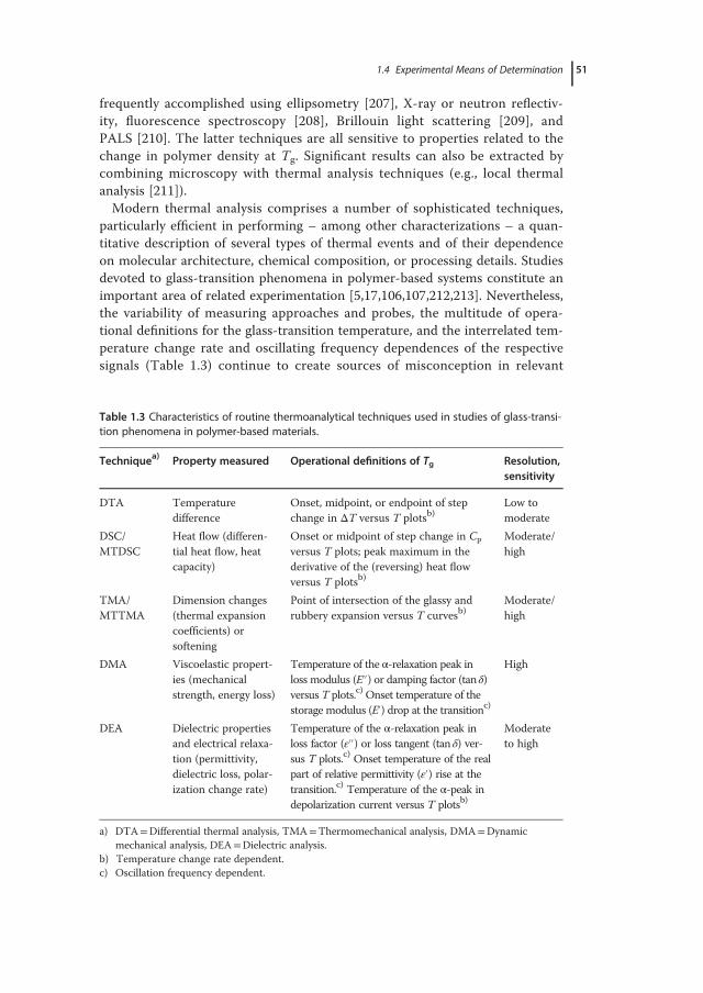
frequently accomplished using ellipsometry [207], X-ray or neutron reflectiv-ity, fluorescence spectroscopy [208], Brillouin light scattering [209], andPALS [210]. The latter techniques are all sensitive to properties related to thechange in polymer density at Tg. Significant results can also be extracted bycombining microscopy with thermal analysis techniques (e.g., local thermalanalysis [211]).Modern thermal analysis comprises a number of sophisticated techniques,

particularly efficient in performing – among other characterizations – a quan-titative description of several types of thermal events and of their dependenceon molecular architecture, chemical composition, or processing details. Studiesdevoted to glass-transition phenomena in polymer-based systems constitute animportant area of related experimentation [5,17,106,107,212,213]. Nevertheless,the variability of measuring approaches and probes, the multitude of opera-tional definitions for the glass-transition temperature, and the interrelated tem-perature change rate and oscillating frequency dependences of the respectivesignals (Table 1.3) continue to create sources of misconception in relevant

Table 1.3 Characteristics of routine thermoanalytical techniques used in studies of glass-transi-tion phenomena in polymer-based materials.

Techniquea) Property measured Operational definitions of Tg Resolution,sensitivity

DTA Temperaturedifference

Onset, midpoint, or endpoint of stepchange in ΔT versus T plotsb)

Low tomoderate

DSC/MTDSC

Heat flow (differen-tial heat flow, heatcapacity)

Onset or midpoint of step change in Cp

versus T plots; peak maximum in thederivative of the (reversing) heat flowversus T plotsb)

Moderate/high

TMA/MTTMA

Dimension changes(thermal expansioncoefficients) orsoftening

Point of intersection of the glassy andrubbery expansion versus T curvesb)

Moderate/high

DMA Viscoelastic propert-ies (mechanicalstrength, energy loss)

Temperature of the α-relaxation peak inloss modulus (E´´) or damping factor (tanδ)versus T plots.c) Onset temperature of thestorage modulus (E´) drop at the transitionc)

High

DEA Dielectric propertiesand electrical relaxa-tion (permittivity,dielectric loss, polar-ization change rate)

Temperature of the α-relaxation peak inloss factor (ε´´) or loss tangent (tan δ) ver-sus T plots.c) Onset temperature of the realpart of relative permittivity (ε´) rise at thetransition.c) Temperature of the α-peak indepolarization current versus T plotsb)

Moderateto high

a) DTA=Differential thermal analysis, TMA=Thermomechanical analysis, DMA=Dynamicmechanical analysis, DEA=Dielectric analysis.

b) Temperature change rate dependent.c) Oscillation frequency dependent.

1.4 Experimental Means of Determination 51

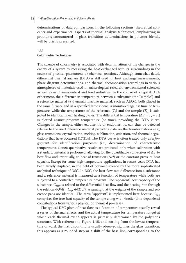
determinations or data comparisons. In the following sections, theoretical con-cepts and experimental aspects of thermal analysis techniques, emphasizing inproblems encountered in glass-transition determinations in polymer blends,will be briefly presented.

1.4.1

Calorimetric Techniques

The science of calorimetry is associated with determinations of the changes in theenergy of a system by measuring the heat exchanged with its surroundings in thecourse of physical phenomena or chemical reactions. Although somewhat dated,differential thermal analysis (DTA) is still used for heat exchange measurements,phase diagram determinations, and thermal decomposition recordings in variousatmospheres of materials used in mineralogical research, environmental sciences,as well as in pharmaceutical and food industries. In the course of a typical DTAexperiment, the difference in temperature between a substance (the “sample”) anda reference material (a thermally inactive material, such as Al2O3), both placed inthe same furnace and in a specified atmosphere, is monitored against time or tem-perature, while the temperature of the reference (Tr) and the sample (Ts) is sub-jected to identical linear heating cycles. The differential temperature (ΔT=Ts�Tr)is plotted against program temperature (or time), providing the DTA curve.Changes in the sample, either exothermic or endothermic, can thus be detectedrelative to the inert reference material providing data on the transformations (e.g.,glass transitions, crystallization, melting, sublimation, oxidation, and thermal degra-dation) that have occurred [17,214]. The DTA curve is often treated only as a fin-gerprint for identification purposes (i.e., determination of characteristictemperatures alone); quantitative results are produced only when calibration witha standard material is performed, allowing for the quantifiable conversion of ΔT toheat flow and, eventually, to heat of transition (ΔH) or the constant pressure heatcapacity. Except for some high-temperature applications, in recent years DTA hasbeen largely displaced in the field of polymer science by the more sophisticatedanalytical technique of DSC. In DSC, the heat flow rate difference into a substanceand a reference material is measured as a function of temperature while both aresubjected to a controlled temperature program. The “apparent” heat capacity of thesubstance, Capp, is related to the differential heat flow and the heating rate throughthe relation dQ/dt=Capp�(dT/dt), assuming that the weights of the sample and ref-erence pans are identical. The term “apparent” is implemented here because Capp

comprises the true heat capacity of the sample along with kinetic (time-dependent)contributions from various physical or chemical processes.The typical DSC plots of heat flow as a function of temperature usually reveal

a series of thermal effects, and the actual temperature (or temperature range) atwhich each thermal event appears is primarily determined by the polymer’sstructure. With reference to Figure 1.15, and starting from the lowest tempera-ture onward, the first discontinuity usually observed signifies the glass transition;this appears as a rounded step or a shift of the base line, corresponding to the


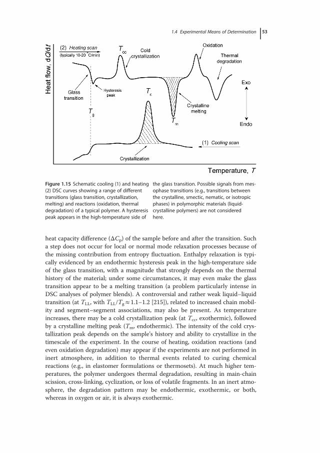
heat capacity difference (ΔCp) of the sample before and after the transition. Sucha step does not occur for local or normal mode relaxation processes because ofthe missing contribution from entropy fluctuation. Enthalpy relaxation is typi-cally evidenced by an endothermic hysteresis peak in the high-temperature sideof the glass transition, with a magnitude that strongly depends on the thermalhistory of the material; under some circumstances, it may even make the glasstransition appear to be a melting transition (a problem particularly intense inDSC analyses of polymer blends). A controversial and rather weak liquid–liquidtransition (at TLL, with TLL/Tg� 1.1–1.2 [215]), related to increased chain mobil-ity and segment–segment associations, may also be present. As temperatureincreases, there may be a cold crystallization peak (at Tcc, exothermic), followedby a crystalline melting peak (Tm, endothermic). The intensity of the cold crys-tallization peak depends on the sample’s history and ability to crystallize in thetimescale of the experiment. In the course of heating, oxidation reactions (andeven oxidation degradation) may appear if the experiments are not performed ininert atmosphere, in addition to thermal events related to curing chemicalreactions (e.g., in elastomer formulations or thermosets). At much higher tem-peratures, the polymer undergoes thermal degradation, resulting in main-chainscission, cross-linking, cyclization, or loss of volatile fragments. In an inert atmo-sphere, the degradation pattern may be endothermic, exothermic, or both,whereas in oxygen or air, it is always exothermic.

Figure 1.15 Schematic cooling (1) and heating(2) DSC curves showing a range of differenttransitions (glass transition, crystallization,melting) and reactions (oxidation, thermaldegradation) of a typical polymer. A hysteresispeak appears in the high-temperature side of

the glass transition. Possible signals from mes-ophase transitions (e.g., transitions betweenthe crystalline, smectic, nematic, or isotropicphases) in polymorphic materials (liquid-crystalline polymers) are not consideredhere.


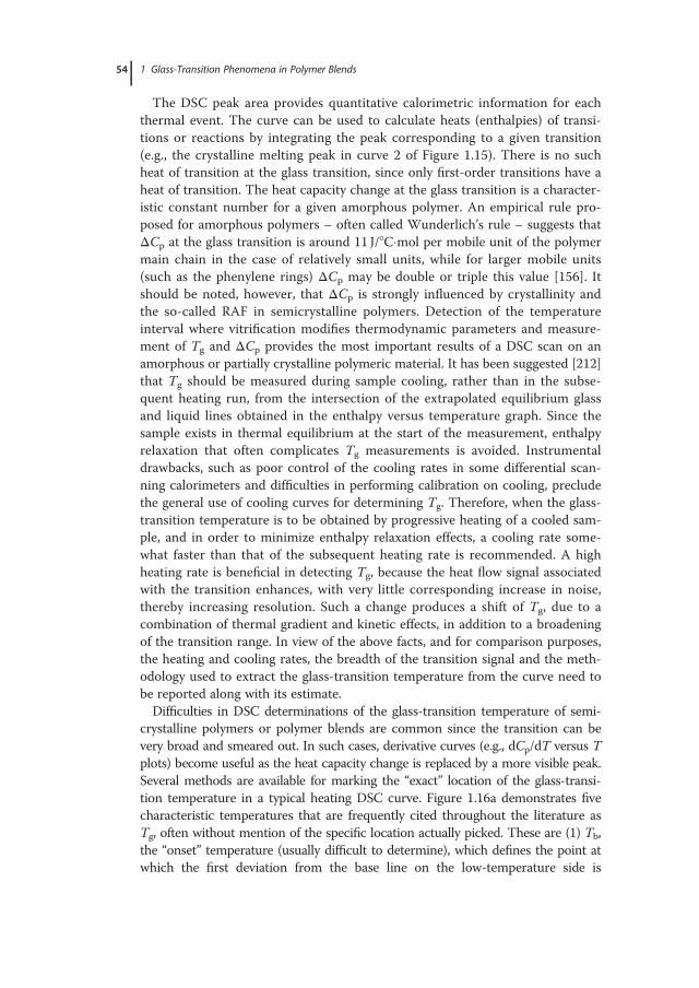
The DSC peak area provides quantitative calorimetric information for eachthermal event. The curve can be used to calculate heats (enthalpies) of transi-tions or reactions by integrating the peak corresponding to a given transition(e.g., the crystalline melting peak in curve 2 of Figure 1.15). There is no suchheat of transition at the glass transition, since only first-order transitions have aheat of transition. The heat capacity change at the glass transition is a character-istic constant number for a given amorphous polymer. An empirical rule pro-posed for amorphous polymers – often called Wunderlich’s rule – suggests thatΔCp at the glass transition is around 11 J/°C�mol per mobile unit of the polymermain chain in the case of relatively small units, while for larger mobile units(such as the phenylene rings) ΔCp may be double or triple this value [156]. Itshould be noted, however, that ΔCp is strongly influenced by crystallinity andthe so-called RAF in semicrystalline polymers. Detection of the temperatureinterval where vitrification modifies thermodynamic parameters and measure-ment of Tg and ΔCp provides the most important results of a DSC scan on anamorphous or partially crystalline polymeric material. It has been suggested [212]that Tg should be measured during sample cooling, rather than in the subse-quent heating run, from the intersection of the extrapolated equilibrium glassand liquid lines obtained in the enthalpy versus temperature graph. Since thesample exists in thermal equilibrium at the start of the measurement, enthalpyrelaxation that often complicates Tg measurements is avoided. Instrumentaldrawbacks, such as poor control of the cooling rates in some differential scan-ning calorimeters and difficulties in performing calibration on cooling, precludethe general use of cooling curves for determining Tg. Therefore, when the glass-transition temperature is to be obtained by progressive heating of a cooled sam-ple, and in order to minimize enthalpy relaxation effects, a cooling rate some-what faster than that of the subsequent heating rate is recommended. A highheating rate is beneficial in detecting Tg, because the heat flow signal associatedwith the transition enhances, with very little corresponding increase in noise,thereby increasing resolution. Such a change produces a shift of Tg, due to acombination of thermal gradient and kinetic effects, in addition to a broadeningof the transition range. In view of the above facts, and for comparison purposes,the heating and cooling rates, the breadth of the transition signal and the meth-odology used to extract the glass-transition temperature from the curve need tobe reported along with its estimate.Difficulties in DSC determinations of the glass-transition temperature of semi-

crystalline polymers or polymer blends are common since the transition can bevery broad and smeared out. In such cases, derivative curves (e.g., dCp/dT versus Tplots) become useful as the heat capacity change is replaced by a more visible peak.Several methods are available for marking the “exact” location of the glass-transi-tion temperature in a typical heating DSC curve. Figure 1.16a demonstrates fivecharacteristic temperatures that are frequently cited throughout the literature asTg, often without mention of the specific location actually picked. These are (1) Tb,the “onset” temperature (usually difficult to determine), which defines the point atwhich the first deviation from the base line on the low-temperature side is


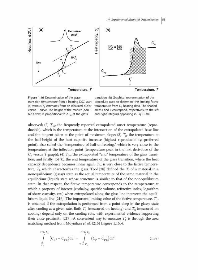
observed; (2) T1e, the frequently reported extrapolated onset temperature (repro-ducible), which is the temperature at the intersection of the extrapolated base lineand the tangent taken at the point of maximum slope; (3) Tg, the temperature atthe half-height of the heat capacity increase (highest reproducibility; preferredpoint), also called the “temperature of half-unfreezing,” which is very close to thetemperature at the inflection point (temperature peak in the first derivative of theCp versus T graph); (4) T2e, the extrapolated “end” temperature of the glass transi-tion; and finally, (5) Te, the end temperature of the glass transition, where the heatcapacity dependence becomes linear again. T1e is very close to the fictive tempera-ture, Tf, which characterizes the glass. Tool [28] defined the Tf of a material in anonequilibrium (glassy) state as the actual temperature of the same material in theequilibrium (liquid) state whose structure is similar to that of the nonequilibriumstate. In that respect, the fictive temperature corresponds to the temperature atwhich a property of interest (enthalpy, specific volume, refractive index, logarithmof shear viscosity, etc.) when extrapolated along the glass line intersects the equili-brium liquid line [216]. The important limiting value of the fictive temperature, T f́ ,is obtained if the extrapolation is performed from a point deep in the glassy stateafter cooling at a given rate. Both T f́ (measured on heating) and Tg (measured oncooling) depend only on the cooling rate, with experimental evidence supportingtheir close proximity [217]. A convenient way to measure T f́ is through the areamatching method from Moynihan et al. [216] (Figure 1.16b),

ZT �T g

T f́

Cp;l � Cp;g� �

dT �ZT �Tg

T �T g

Cp � Cp;g� �

dT : (1.38)

Figure 1.16 Determination of the glass-transition temperature from a heating DSC scan:(a) various Tg estimates from an idealized dQ/dtversus T curve. The height of the marker (dou-ble arrow) is proportional to ΔCp at the glass

transition. (b) Graphical representation of theprocedure used to determine the limiting fictivetemperature from Cp heating data. The shadedareas I and II correspond, respectively, to the leftand right integrals appearing in Eq. (1.38).


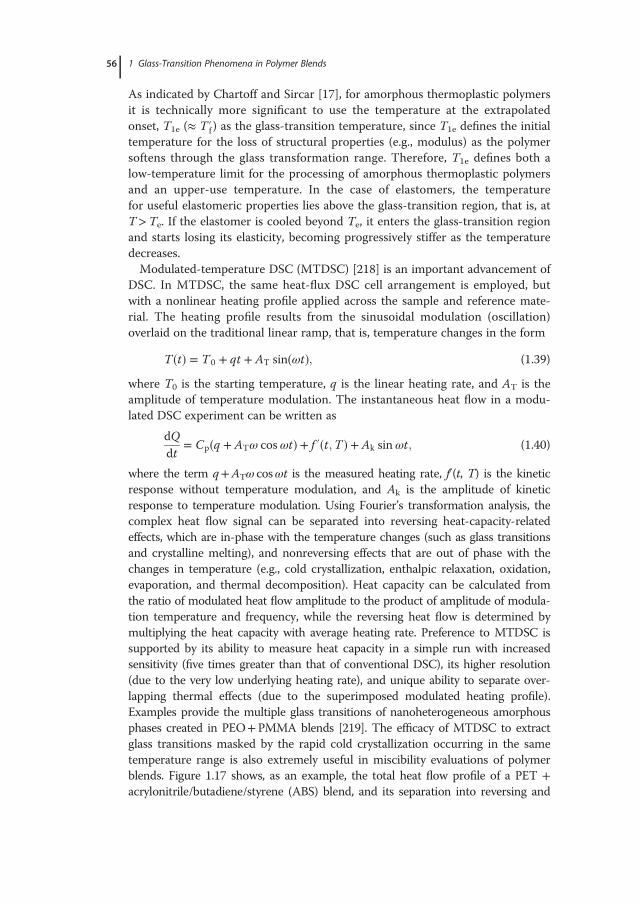
As indicated by Chartoff and Sircar [17], for amorphous thermoplastic polymersit is technically more significant to use the temperature at the extrapolatedonset, T1e (� T f́ ) as the glass-transition temperature, since T1e defines the initialtemperature for the loss of structural properties (e.g., modulus) as the polymersoftens through the glass transformation range. Therefore, T1e defines both alow-temperature limit for the processing of amorphous thermoplastic polymersand an upper-use temperature. In the case of elastomers, the temperaturefor useful elastomeric properties lies above the glass-transition region, that is, atT>Te. If the elastomer is cooled beyond Te, it enters the glass-transition regionand starts losing its elasticity, becoming progressively stiffer as the temperaturedecreases.Modulated-temperature DSC (MTDSC) [218] is an important advancement of

DSC. In MTDSC, the same heat-flux DSC cell arrangement is employed, butwith a nonlinear heating profile applied across the sample and reference mate-rial. The heating profile results from the sinusoidal modulation (oscillation)overlaid on the traditional linear ramp, that is, temperature changes in the form

T �t� � T 0 � qt � AT sin�ωt�; (1.39)

where T0 is the starting temperature, q is the linear heating rate, and AT is theamplitude of temperature modulation. The instantaneous heat flow in a modu-lated DSC experiment can be written as

dQdt

� Cp�q � ATω cosωt� � f ´�t;T � � Ak sinωt; (1.40)

where the term q+ATω cosωt is the measured heating rate, f´(t, T) is the kineticresponse without temperature modulation, and Ak is the amplitude of kineticresponse to temperature modulation. Using Fourier’s transformation analysis, thecomplex heat flow signal can be separated into reversing heat-capacity-relatedeffects, which are in-phase with the temperature changes (such as glass transitionsand crystalline melting), and nonreversing effects that are out of phase with thechanges in temperature (e.g., cold crystallization, enthalpic relaxation, oxidation,evaporation, and thermal decomposition). Heat capacity can be calculated fromthe ratio of modulated heat flow amplitude to the product of amplitude of modula-tion temperature and frequency, while the reversing heat flow is determined bymultiplying the heat capacity with average heating rate. Preference to MTDSC issupported by its ability to measure heat capacity in a simple run with increasedsensitivity (five times greater than that of conventional DSC), its higher resolution(due to the very low underlying heating rate), and unique ability to separate over-lapping thermal effects (due to the superimposed modulated heating profile).Examples provide the multiple glass transitions of nanoheterogeneous amorphousphases created in PEO+PMMA blends [219]. The efficacy of MTDSC to extractglass transitions masked by the rapid cold crystallization occurring in the sametemperature range is also extremely useful in miscibility evaluations of polymerblends. Figure 1.17 shows, as an example, the total heat flow profile of a PET +acrylonitrile/butadiene/styrene (ABS) blend, and its separation into reversing and


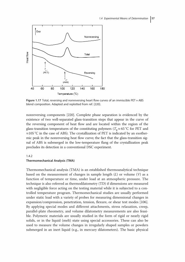
nonreversing components [220]. Complete phase separation is evidenced by theexistence of two well-separated glass-transition steps that appear in the curve ofthe reversing component of heat flow and are located within the region of theglass-transition temperatures of the constituting polymers (Tg� 65 °C for PET and�105 °C in the case of ABS). The crystallization of PET is indicated by an exother-mic peak in the nonreversing heat flow curve; the fact that the glass-transition sig-nal of ABS is submerged in the low-temperature flang of the crystallization peakprecludes its detection in a conventional DSC experiment.

1.4.2

Thermomechanical Analysis (TMA)

Thermomechanical analysis (TMA) is an established thermoanalytical techniquebased on the measurement of changes in sample length (L) or volume (V) as afunction of temperature or time, under load at an atmospheric pressure. Thetechnique is also referred as thermodilatometry (TD) if dimensions are measuredwith negligible force acting on the testing material while it is subjected to a con-trolled temperature program. Thermomechanical studies are usually performedunder static load with a variety of probes for measuring dimensional changes inexpansion/compression, penetration, tension, flexure, or shear test modes [106].By applying special modes and different attachments, stress relaxation, creep,parallel-plate rheometry, and volume dilatometry measurements are also feasi-ble. Polymeric materials are usually studied in the form of rigid or nearly rigidsolids, or in the liquid (melt) state using special accessories. These can also beused to measure the volume changes in irregularly shaped samples or powderssubmerged in an inert liquid (e.g., in mercury dilatometers). The basic physical

Figure 1.17 Total, reversing and nonreversing heart flow curves of an immiscible PET+ABSblend composition. Adapted and replotted from ref. [220].


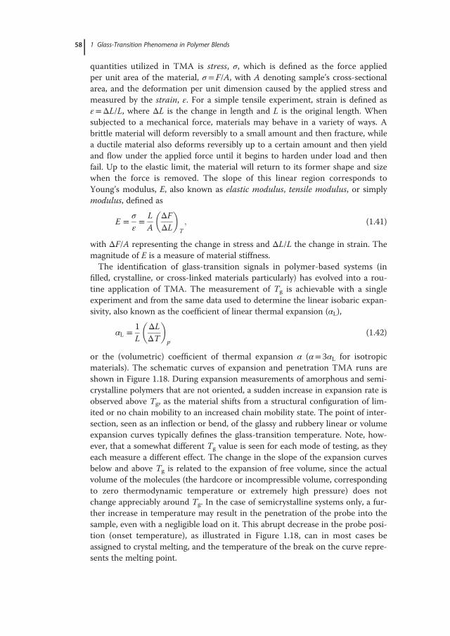
quantities utilized in TMA is stress, σ, which is defined as the force appliedper unit area of the material, σ = F/A, with A denoting sample’s cross-sectionalarea, and the deformation per unit dimension caused by the applied stress andmeasured by the strain, ε. For a simple tensile experiment, strain is defined asε=ΔL/L, where ΔL is the change in length and L is the original length. Whensubjected to a mechanical force, materials may behave in a variety of ways. Abrittle material will deform reversibly to a small amount and then fracture, whilea ductile material also deforms reversibly up to a certain amount and then yieldand flow under the applied force until it begins to harden under load and thenfail. Up to the elastic limit, the material will return to its former shape and sizewhen the force is removed. The slope of this linear region corresponds toYoung’s modulus, E, also known as elastic modulus, tensile modulus, or simplymodulus, defined as

E � σ

ε� LA

ΔFΔL

� �T

; (1.41)

with ΔF/A representing the change in stress and ΔL/L the change in strain. Themagnitude of E is a measure of material stiffness.The identification of glass-transition signals in polymer-based systems (in

filled, crystalline, or cross-linked materials particularly) has evolved into a rou-tine application of TMA. The measurement of Tg is achievable with a singleexperiment and from the same data used to determine the linear isobaric expan-sivity, also known as the coefficient of linear thermal expansion (αL),

αL � 1L

ΔLΔT

� �p

(1.42)

or the (volumetric) coefficient of thermal expansion α (α= 3αL for isotropicmaterials). The schematic curves of expansion and penetration TMA runs areshown in Figure 1.18. During expansion measurements of amorphous and semi-crystalline polymers that are not oriented, a sudden increase in expansion rate isobserved above Tg, as the material shifts from a structural configuration of lim-ited or no chain mobility to an increased chain mobility state. The point of inter-section, seen as an inflection or bend, of the glassy and rubbery linear or volumeexpansion curves typically defines the glass-transition temperature. Note, how-ever, that a somewhat different Tg value is seen for each mode of testing, as theyeach measure a different effect. The change in the slope of the expansion curvesbelow and above Tg is related to the expansion of free volume, since the actualvolume of the molecules (the hardcore or incompressible volume, correspondingto zero thermodynamic temperature or extremely high pressure) does notchange appreciably around Tg. In the case of semicrystalline systems only, a fur-ther increase in temperature may result in the penetration of the probe into thesample, even with a negligible load on it. This abrupt decrease in the probe posi-tion (onset temperature), as illustrated in Figure 1.18, can in most cases beassigned to crystal melting, and the temperature of the break on the curve repre-sents the melting point.


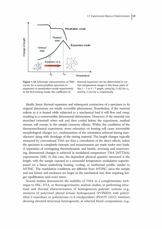
Ideally, linear thermal expansion and subsequent contraction of a specimen to itsoriginal dimensions are totally reversible phenomena. Nonetheless, if the materialsoftens as it is heated while subjected to a mechanical load it will flow and creep,resulting in a nonreversible dimensional deformation. Moreover, if the material wasstretched (oriented) when soft and then cooled before the experiment, residualstresses will remain in the sample (memory effects). Within the conditions of thethermomechanical experiment, stress relaxation on heating will cause irreversiblemorphological changes (i.e., randomization of the orientation achieved during man-ufacture) along with shrinkage of the testing material. The length changes typicallymeasured by conventional TMA are thus a convolution of the above effects, unlessthe specimen is completely isotropic and measurements are made under zero loads.A separation of overlapping thermodynamic and kinetic, reversing and nonrevers-ing, dimensional changes is achieved in modulated temperature TMA (MTTMA)experiments [106]. In this case, the dependent physical quantity measured is thelength, with the sample exposed to a sinusoidal temperature modulation superim-posed on a linear underlying heating, cooling, or isothermal profile, similar toMTDSC. The modulation conditions are different from MTDSC, since the sampleand test fixture and enclosure are larger in the mechanical test, thus requiring lon-ger equilibration (and scan) times.Several studies demonstrate the usability of TMA as a complementary tech-

nique to DSC, DTA, or thermogravimetric analysis studies, in performing struc-tural and thermal characterization of homogeneous polymer systems (e.g.,mixtures of poly(vinyl phenyl ketone hydrogenated (PVPhKH) with poly(2-ethyl-2-oxazoline) or poly(styrene-co-4-vinylpyridine) (PS4VP) [221]), mixturesshowing elevated structural heterogeneity at selected blend compositions (e.g.,

Figure 1.18 Schematic representation of TMAcurves for a semicrystalline specimen inexpansion or penetration-mode experiments.In the first testing mode, the coefficient of

thermal expansion can be determined in cer-tain temperature ranges in the linear parts ofthe L� T or V� T graph, using Eq. (1.42) for αL,and Eq. (1.2c) for α, respectively.


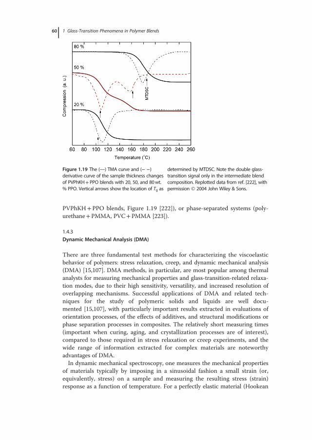
PVPhKH+PPO blends, Figure 1.19 [222]), or phase-separated systems (poly-urethane+PMMA, PVC+PMMA [223]).

1.4.3

Dynamic Mechanical Analysis (DMA)

There are three fundamental test methods for characterizing the viscoelasticbehavior of polymers: stress relaxation, creep, and dynamic mechanical analysis(DMA) [15,107]. DMA methods, in particular, are most popular among thermalanalysts for measuring mechanical properties and glass-transition-related relaxa-tion modes, due to their high sensitivity, versatility, and increased resolution ofoverlapping mechanisms. Successful applications of DMA and related tech-niques for the study of polymeric solids and liquids are well docu-mented [15,107], with particularly important results extracted in evaluations oforientation processes, of the effects of additives, and structural modifications orphase separation processes in composites. The relatively short measuring times(important when curing, aging, and crystallization processes are of interest),compared to those required in stress relaxation or creep experiments, and thewide range of information extracted for complex materials are noteworthyadvantages of DMA.In dynamic mechanical spectroscopy, one measures the mechanical properties

of materials typically by imposing in a sinusoidal fashion a small strain (or,equivalently, stress) on a sample and measuring the resulting stress (strain)response as a function of temperature. For a perfectly elastic material (Hookean

Figure 1.19 The (—) TMA curve and (� �)derivative curve of the sample thickness changesof PVPhKH+ PPO blends with 20, 50, and 80wt.% PPO. Vertical arrows show the location of Tg as

determined by MTDSC. Note the double glass-transition signal only in the intermediate blendcomposition. Replotted data from ref. [222], withpermission 2004 John Wiley & Sons.


solid), stress and strain are in phase. In an ideal liquid behavior (Newtonianfluid), however, instead of deforming reversibly under load the material willflow; the strain is now proportional to the rate of change of the stress. The phaseangle difference of δ= 90° between sinusoidal stress and strain in liquids is thekey for the use of DMA as a tool in the characterization of viscoelastic polymers.Since such materials have properties intermediate between those of an ideal solidand an ideal liquid, they will exhibit a phase lag (δ) somewhere between 0° (idealsolid) and 90° (ideal liquid). Along these lines, an application of a sinusoidalforce (strain) to the testing material,

ε�t� � εmax?sin�ωt�; (1.43a)

where ω denotes the angular frequency, produces a stress of the form

σ�t� � σmax?sin�ωt � δ�: (1.43b)

The relative amplitudes of stress and strain and the phase lag, which reflects therelative degree of viscous character to elastic character, can thus be obtained.DMA data are commonly reported using the complex modulus function

E∗ � σ�t�ε�t� �

σmaxei�ωt�δ�εmaxeiωt

� σmax

εmax

� �eiδ � σmax

εmaxcos�δ� � i sin�δ�� E´ � iE´´:

(1.44)

Its real component, E´, is known as the storage modulus and is a measure of theelastic character or solid-like nature of the material. The imaginary part, E´´, isknown as the loss modulus and is a measure of the viscous character or liquid-like nature of the material. In a physical sense, the first is related to the stiffnessof the material, and the latter reflects the damping capacity of the material. Foran ideal elastic solid, E´ is simply Young’s modulus of the material and E´´ is zero,while for an ideal viscous liquid E´ is zero and the loss modulus is related to theviscosity of the material. The ratio of the loss modulus to the storage modulus isknown as the damping factor or loss tangent, or, more commonly, as

tan δ � E´´E´ : (1.45)

Tan δ ranges from zero for an ideal elastic solid to infinity for an ideal liquid, andrepresents the ratio of energy dissipated to energy stored per cycle of deforma-tion. Analogous definitions apply for the parameters used in tests under a shearmode of deformation (i.e., the complex shear modulus G∗ and tan δ=G´´/G´) andrheological measurements in polymer liquids [107].The dynamic mechanical data obtained for polymer-based systems convey

information on a broad range of relaxation processes, that goes from very localmotions (secondary relaxations, generally due to branching chains or sidechains) to segmental mobility exhibiting cooperativity (α-relaxation or dynamicglass transition), or even large-scale relaxation processes (Rouse dynamics orreptation) [224]. Thermal analysts usually perform a series of temperature scansat a constant oscillatory frequency, covering a narrow range of frequencies


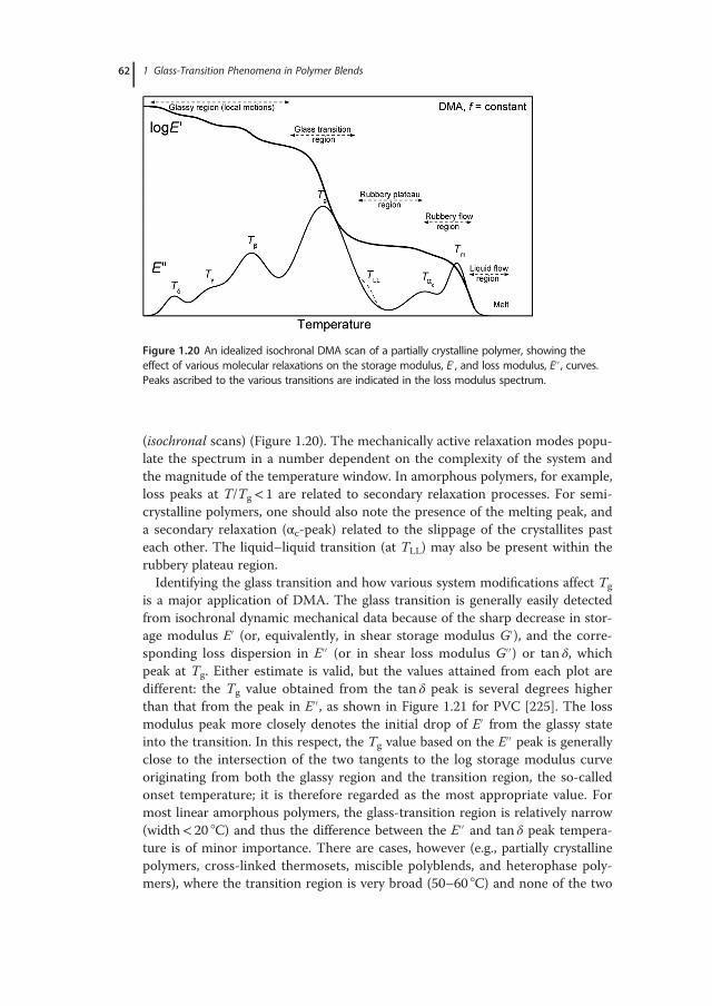
(isochronal scans) (Figure 1.20). The mechanically active relaxation modes popu-late the spectrum in a number dependent on the complexity of the system andthe magnitude of the temperature window. In amorphous polymers, for example,loss peaks at T/Tg< 1 are related to secondary relaxation processes. For semi-crystalline polymers, one should also note the presence of the melting peak, anda secondary relaxation (αc-peak) related to the slippage of the crystallites pasteach other. The liquid–liquid transition (at TLL) may also be present within therubbery plateau region.Identifying the glass transition and how various system modifications affect Tg

is a major application of DMA. The glass transition is generally easily detectedfrom isochronal dynamic mechanical data because of the sharp decrease in stor-age modulus E´ (or, equivalently, in shear storage modulus G´), and the corre-sponding loss dispersion in E´´ (or in shear loss modulus G´´) or tan δ, whichpeak at Tg. Either estimate is valid, but the values attained from each plot aredifferent: the Tg value obtained from the tan δ peak is several degrees higherthan that from the peak in E´´, as shown in Figure 1.21 for PVC [225]. The lossmodulus peak more closely denotes the initial drop of E´ from the glassy stateinto the transition. In this respect, the Tg value based on the E´´ peak is generallyclose to the intersection of the two tangents to the log storage modulus curveoriginating from both the glassy region and the transition region, the so-calledonset temperature; it is therefore regarded as the most appropriate value. Formost linear amorphous polymers, the glass-transition region is relatively narrow(width< 20 °C) and thus the difference between the E´´ and tan δ peak tempera-ture is of minor importance. There are cases, however (e.g., partially crystallinepolymers, cross-linked thermosets, miscible polyblends, and heterophase poly-mers), where the transition region is very broad (50–60 °C) and none of the two

Figure 1.20 An idealized isochronal DMA scan of a partially crystalline polymer, showing theeffect of various molecular relaxations on the storage modulus, E´ , and loss modulus, E´´ , curves.Peaks ascribed to the various transitions are indicated in the loss modulus spectrum.


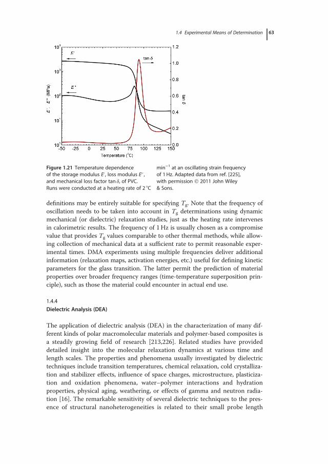
definitions may be entirely suitable for specifying Tg. Note that the frequency ofoscillation needs to be taken into account in Tg determinations using dynamicmechanical (or dielectric) relaxation studies, just as the heating rate intervenesin calorimetric results. The frequency of 1Hz is usually chosen as a compromisevalue that provides Tg values comparable to other thermal methods, while allow-ing collection of mechanical data at a sufficient rate to permit reasonable exper-imental times. DMA experiments using multiple frequencies deliver additionalinformation (relaxation maps, activation energies, etc.) useful for defining kineticparameters for the glass transition. The latter permit the prediction of materialproperties over broader frequency ranges (time-temperature superposition prin-ciple), such as those the material could encounter in actual end use.

1.4.4

Dielectric Analysis (DEA)

The application of dielectric analysis (DEA) in the characterization of many dif-ferent kinds of polar macromolecular materials and polymer-based composites isa steadily growing field of research [213,226]. Related studies have provideddetailed insight into the molecular relaxation dynamics at various time andlength scales. The properties and phenomena usually investigated by dielectrictechniques include transition temperatures, chemical relaxation, cold crystalliza-tion and stabilizer effects, influence of space charges, microstructure, plasticiza-tion and oxidation phenomena, water–polymer interactions and hydrationproperties, physical aging, weathering, or effects of gamma and neutron radia-tion [16]. The remarkable sensitivity of several dielectric techniques to the pres-ence of structural nanoheterogeneities is related to their small probe length

Figure 1.21 Temperature dependenceof the storage modulus E´ , loss modulus E´´ ,and mechanical loss factor tan δ, of PVC.Runs were conducted at a heating rate of 2 °C

min�1 at an oscillating strain frequencyof 1 Hz. Adapted data from ref. [225],with permission 2011 John Wiley& Sons.


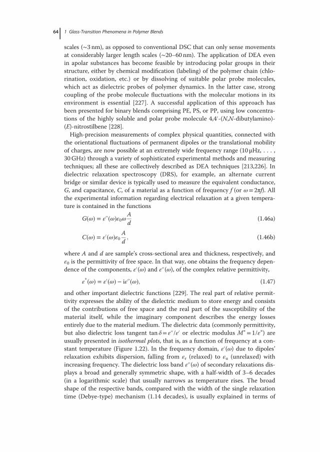
scales (∼3 nm), as opposed to conventional DSC that can only sense movementsat considerably larger length scales (∼20–60 nm). The application of DEA evenin apolar substances has become feasible by introducing polar groups in theirstructure, either by chemical modification (labeling) of the polymer chain (chlo-rination, oxidation, etc.) or by dissolving of suitable polar probe molecules,which act as dielectric probes of polymer dynamics. In the latter case, strongcoupling of the probe molecule fluctuations with the molecular motions in itsenvironment is essential [227]. A successful application of this approach hasbeen presented for binary blends comprising PE, PS, or PP, using low concentra-tions of the highly soluble and polar probe molecule 4,4´-(N,N-dibutylamino)-(E)-nitrostilbene [228].High-precision measurements of complex physical quantities, connected with

the orientational fluctuations of permanent dipoles or the translational mobilityof charges, are now possible at an extremely wide frequency range (10 μHz, . . . ,30GHz) through a variety of sophisticated experimental methods and measuringtechniques; all these are collectively described as DEA techniques [213,226]. Indielectric relaxation spectroscopy (DRS), for example, an alternate currentbridge or similar device is typically used to measure the equivalent conductance,G, and capacitance, C, of a material as a function of frequency f (or ω= 2πf). Allthe experimental information regarding electrical relaxation at a given tempera-ture is contained in the functions

G�ω� � ε´´�ω�ε0ωAd

(1.46a)

C�ω� � ε´�ω�ε0 Ad ; (1.46b)

where A and d are sample’s cross-sectional area and thickness, respectively, andε0 is the permittivity of free space. In that way, one obtains the frequency depen-dence of the components, ε´(ω) and ε´´(ω), of the complex relative permittivity,

ε��ω� � ε´�ω� � iε´´�ω�; (1.47)

and other important dielectric functions [229]. The real part of relative permit-tivity expresses the ability of the dielectric medium to store energy and consistsof the contributions of free space and the real part of the susceptibility of thematerial itself, while the imaginary component describes the energy lossesentirely due to the material medium. The dielectric data (commonly permittivity,but also dielectric loss tangent tan δ= ε´´/ε´ or electric modulus M∗= 1/ε∗) areusually presented in isothermal plots, that is, as a function of frequency at a con-stant temperature (Figure 1.22). In the frequency domain, ε´(ω) due to dipoles’relaxation exhibits dispersion, falling from εr (relaxed) to εu (unrelaxed) withincreasing frequency. The dielectric loss band ε´´(ω) of secondary relaxations dis-plays a broad and generally symmetric shape, with a half-width of 3–6 decades(in a logarithmic scale) that usually narrows as temperature rises. The broadshape of the respective bands, compared with the width of the single relaxationtime (Debye-type) mechanism (1.14 decades), is usually explained in terms of


a distribution of environments in which the molecular entities relax. Theα-relaxation (glass transition) displays a relatively broad but asymmetric shape,with a half-width of 2–5 decades. Permittivity data collected at some tempera-ture are typically analyzed by a superposition of several Havriliak and Negami(HN) functions [230] and a conductivity term,

ε�exp�ω� � ε1 �Xi

Δεi1 � iωτHN� �1�αHN;i� �βHN;i

� iσdcε0ωp

; (1.48)

where σdc is the dc conductivity of the material (p= 1 for purely ohmic conduc-tivity). The shape parameters 0� αHN< 1 and 0< βHN� 1 describe the width andthe asymmetry of the loss peak, respectively, and with the addition of thedielectric strength Δε= εr� εu and τHN (a parameter directly related to the relax-ation time τ) provide a complete description of each relaxation process. Thedielectric glass-transition temperature (Tg,diel) is defined by the conventionτα(Tg,diel)= 100 s, and corresponds to the temperature at which the maximum ofthe loss factor band is located at the frequency of fmax,α= 1.6× 10�3Hz. As withDMA, dielectric relaxation data can also be plotted as a function of temperatureat a constant frequency (isochronal plots). Current-temperature (I(T)) spectra,resembling the isochronal ε´´(T) plots, are collected using the thermally stimu-lated (depolarization) currents (thermally stimulated currents [TSC] or thermallystimulated depolarization currents [TSDC]) technique. The equivalent frequencyof this technique is in the range 10�4–10�2Hz, depending on the rate used forsample heating [213], and is sufficiently low to permit increased resolution ofthe complex signals recorded in polymer composites. In both cases, an

Figure 1.22 Generic behavior of frequencydependence of permittivity components(ε´ and ε´´) for the typical dielectric relaxationmodes in glassy polymers and relatedcomposites. Interfacial polarization effects are

common in heterogeneous materials (e.g.,immiscible or partially miscible polymerblends), while crystalline phases and additivesare potential sources of additional relaxations.


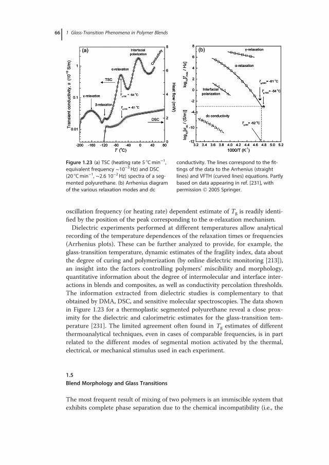
oscillation frequency (or heating rate) dependent estimate of Tg is readily identi-fied by the position of the peak corresponding to the α-relaxation mechanism.Dielectric experiments performed at different temperatures allow analytical

recording of the temperature dependences of the relaxation times or frequencies(Arrhenius plots). These can be further analyzed to provide, for example, theglass-transition temperature, dynamic estimates of the fragility index, data aboutthe degree of curing and polymerization (by online dielectric monitoring [213]),an insight into the factors controlling polymers’ miscibility and morphology,quantitative information about the degree of intermolecular and interface inter-actions in blends and composites, as well as conductivity percolation thresholds.The information extracted from dielectric studies is complementary to thatobtained by DMA, DSC, and sensitive molecular spectroscopies. The data shownin Figure 1.23 for a thermoplastic segmented polyurethane reveal a close prox-imity for the dielectric and calorimetric estimates for the glass-transition tem-perature [231]. The limited agreement often found in Tg estimates of differentthermoanalytical techniques, even in cases of comparable frequencies, is in partrelated to the different modes of segmental motion activated by the thermal,electrical, or mechanical stimulus used in each experiment.

1.5Blend Morphology and Glass Transitions

The most frequent result of mixing of two polymers is an immiscible system thatexhibits complete phase separation due to the chemical incompatibility (i.e., the

Figure 1.23 (a) TSC (heating rate 5 °Cmin�1,equivalent frequency ∼10�3 Hz) and DSC(20 °Cmin�1, ∼2.6 10�2 Hz) spectra of a seg-mented polyurethane. (b) Arrhenius diagramof the various relaxation modes and dc

conductivity. The lines correspond to the fit-tings of the data to the Arrhenius (straightlines) and VFTH (curved lines) equations. Partlybased on data appearing in ref. [231], withpermission 2005 Springer.


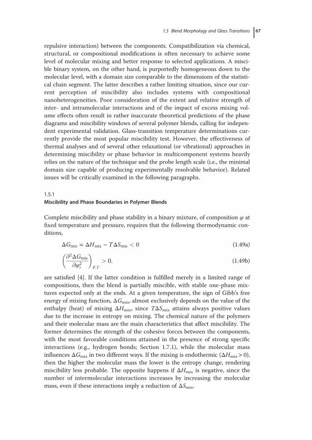
repulsive interaction) between the components. Compatibilization via chemical,structural, or compositional modifications is often necessary to achieve somelevel of molecular mixing and better response to selected applications. A misci-ble binary system, on the other hand, is purportedly homogeneous down to themolecular level, with a domain size comparable to the dimensions of the statisti-cal chain segment. The latter describes a rather limiting situation, since our cur-rent perception of miscibility also includes systems with compositionalnanoheterogeneities. Poor consideration of the extent and relative strength ofinter- and intramolecular interactions and of the impact of excess mixing vol-ume effects often result in rather inaccurate theoretical predictions of the phasediagrams and miscibility windows of several polymer blends, calling for indepen-dent experimental validation. Glass-transition temperature determinations cur-rently provide the most popular miscibility test. However, the effectiveness ofthermal analyses and of several other relaxational (or vibrational) approaches indetermining miscibility or phase behavior in multicomponent systems heavilyrelies on the nature of the technique and the probe length scale (i.e., the minimaldomain size capable of producing experimentally resolvable behavior). Relatedissues will be critically examined in the following paragraphs.

1.5.1

Miscibility and Phase Boundaries in Polymer Blends

Complete miscibility and phase stability in a binary mixture, of composition φ atfixed temperature and pressure, requires that the following thermodynamic con-ditions,

ΔGmix � ΔHmix � TΔSmix < 0 (1.49a)

@2ΔGmix

@φ2i

� �P;T

> 0; (1.49b)

are satisfied [4]. If the latter condition is fulfilled merely in a limited range ofcompositions, then the blend is partially miscible, with stable one-phase mix-tures expected only at the ends. At a given temperature, the sign of Gibb’s freeenergy of mixing function, ΔGmix, almost exclusively depends on the value of theenthalpy (heat) of mixing ΔHmix, since TΔSmix attains always positive valuesdue to the increase in entropy on mixing. The chemical nature of the polymersand their molecular mass are the main characteristics that affect miscibility. Theformer determines the strength of the cohesive forces between the components,with the most favorable conditions attained in the presence of strong specificinteractions (e.g., hydrogen bonds; Section 1.7.1), while the molecular massinfluences ΔGmix in two different ways. If the mixing is endothermic (ΔHmix> 0),then the higher the molecular mass the lower is the entropy change, renderingmiscibility less probable. The opposite happens if ΔHmix is negative, since thenumber of intermolecular interactions increases by increasing the molecularmass, even if these interactions imply a reduction of ΔSmix.

1.5 Blend Morphology and Glass Transitions 67

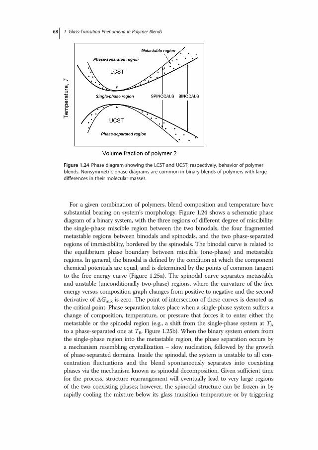
For a given combination of polymers, blend composition and temperature havesubstantial bearing on system’s morphology. Figure 1.24 shows a schematic phasediagram of a binary system, with the three regions of different degree of miscibility:the single-phase miscible region between the two binodals, the four fragmentedmetastable regions between binodals and spinodals, and the two phase-separatedregions of immiscibility, bordered by the spinodals. The binodal curve is related tothe equilibrium phase boundary between miscible (one-phase) and metastableregions. In general, the binodal is defined by the condition at which the componentchemical potentials are equal, and is determined by the points of common tangentto the free energy curve (Figure 1.25a). The spinodal curve separates metastableand unstable (unconditionally two-phase) regions, where the curvature of the freeenergy versus composition graph changes from positive to negative and the secondderivative of ΔGmix is zero. The point of intersection of these curves is denoted asthe critical point. Phase separation takes place when a single-phase system suffers achange of composition, temperature, or pressure that forces it to enter either themetastable or the spinodal region (e.g., a shift from the single-phase system at TA

to a phase-separated one at TB, Figure 1.25b). When the binary system enters fromthe single-phase region into the metastable region, the phase separation occurs bya mechanism resembling crystallization – slow nucleation, followed by the growthof phase-separated domains. Inside the spinodal, the system is unstable to all con-centration fluctuations and the blend spontaneously separates into coexistingphases via the mechanism known as spinodal decomposition. Given sufficient timefor the process, structure rearrangement will eventually lead to very large regionsof the two coexisting phases; however, the spinodal structure can be frozen-in byrapidly cooling the mixture below its glass-transition temperature or by triggering

Figure 1.24 Phase diagram showing the LCST and UCST, respectively, behavior of polymerblends. Nonsymmetric phase diagrams are common in binary blends of polymers with largedifferences in their molecular masses.


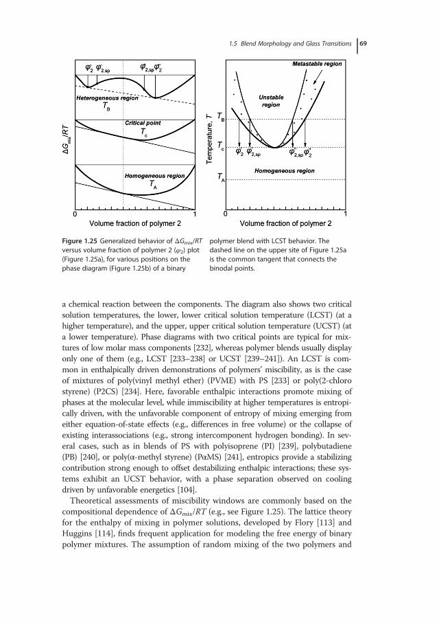
a chemical reaction between the components. The diagram also shows two criticalsolution temperatures, the lower, lower critical solution temperature (LCST) (at ahigher temperature), and the upper, upper critical solution temperature (UCST) (ata lower temperature). Phase diagrams with two critical points are typical for mix-tures of low molar mass components [232], whereas polymer blends usually displayonly one of them (e.g., LCST [233–238] or UCST [239–241]). An LCST is com-mon in enthalpically driven demonstrations of polymers’ miscibility, as is the caseof mixtures of poly(vinyl methyl ether) (PVME) with PS [233] or poly(2-chlorostyrene) (P2CS) [234]. Here, favorable enthalpic interactions promote mixing ofphases at the molecular level, while immiscibility at higher temperatures is entropi-cally driven, with the unfavorable component of entropy of mixing emerging fromeither equation-of-state effects (e.g., differences in free volume) or the collapse ofexisting interassociations (e.g., strong intercomponent hydrogen bonding). In sev-eral cases, such as in blends of PS with polyisoprene (PI) [239], polybutadiene(PB) [240], or poly(α-methyl styrene) (PαMS) [241], entropics provide a stabilizingcontribution strong enough to offset destabilizing enthalpic interactions; these sys-tems exhibit an UCST behavior, with a phase separation observed on coolingdriven by unfavorable energetics [104].Theoretical assessments of miscibility windows are commonly based on the

compositional dependence of ΔGmix/RT (e.g., see Figure 1.25). The lattice theoryfor the enthalpy of mixing in polymer solutions, developed by Flory [113] andHuggins [114], finds frequent application for modeling the free energy of binarypolymer mixtures. The assumption of random mixing of the two polymers and

Figure 1.25 Generalized behavior of ΔGmix/RTversus volume fraction of polymer 2 (φ2) plot(Figure 1.25a), for various positions on thephase diagram (Figure 1.25b) of a binary

polymer blend with LCST behavior. Thedashed line on the upper site of Figure 1.25ais the common tangent that connects thebinodal points.


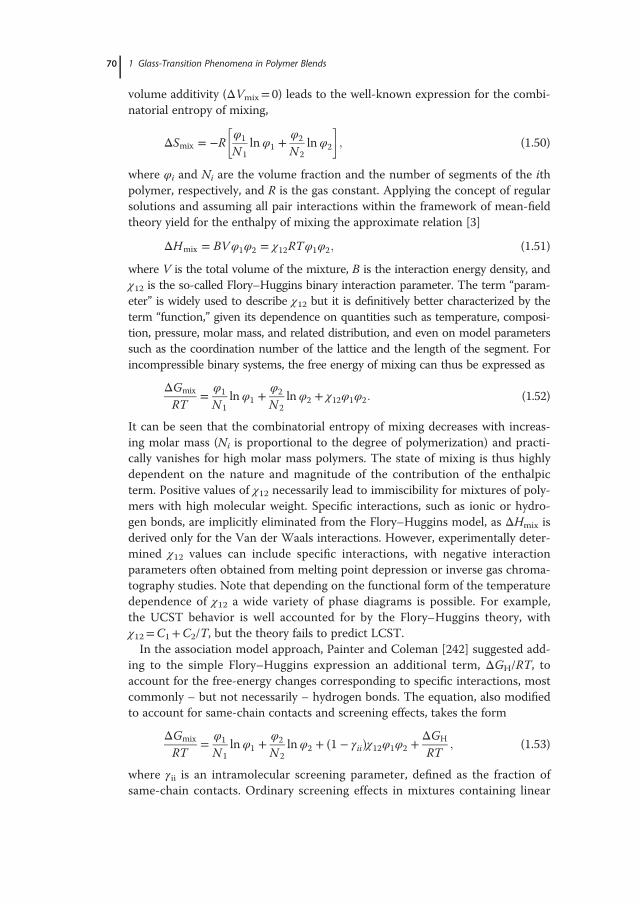
volume additivity (ΔVmix= 0) leads to the well-known expression for the combi-natorial entropy of mixing,

ΔSmix � �R φ1

N1ln φ1 � φ2

N2ln φ2

; (1.50)

where φi and Ni are the volume fraction and the number of segments of the ithpolymer, respectively, and R is the gas constant. Applying the concept of regularsolutions and assuming all pair interactions within the framework of mean-fieldtheory yield for the enthalpy of mixing the approximate relation [3]

ΔHmix � BVφ1φ2 � χ12RTφ1φ2; (1.51)

where V is the total volume of the mixture, B is the interaction energy density, andχ12 is the so-called Flory–Huggins binary interaction parameter. The term “param-eter” is widely used to describe χ12 but it is definitively better characterized by theterm “function,” given its dependence on quantities such as temperature, composi-tion, pressure, molar mass, and related distribution, and even on model parameterssuch as the coordination number of the lattice and the length of the segment. Forincompressible binary systems, the free energy of mixing can thus be expressed as

ΔGmix

RT� φ1

N1ln φ1 � φ2

N2ln φ2 � χ12φ1φ2: (1.52)

It can be seen that the combinatorial entropy of mixing decreases with increas-ing molar mass (Ni is proportional to the degree of polymerization) and practi-cally vanishes for high molar mass polymers. The state of mixing is thus highlydependent on the nature and magnitude of the contribution of the enthalpicterm. Positive values of χ12 necessarily lead to immiscibility for mixtures of poly-mers with high molecular weight. Specific interactions, such as ionic or hydro-gen bonds, are implicitly eliminated from the Flory–Huggins model, as ΔHmix isderived only for the Van der Waals interactions. However, experimentally deter-mined χ12 values can include specific interactions, with negative interactionparameters often obtained from melting point depression or inverse gas chroma-tography studies. Note that depending on the functional form of the temperaturedependence of χ12 a wide variety of phase diagrams is possible. For example,the UCST behavior is well accounted for by the Flory–Huggins theory, withχ12=C1+C2/T, but the theory fails to predict LCST.In the association model approach, Painter and Coleman [242] suggested add-

ing to the simple Flory–Huggins expression an additional term, ΔGH/RT, toaccount for the free-energy changes corresponding to specific interactions, mostcommonly – but not necessarily – hydrogen bonds. The equation, also modifiedto account for same-chain contacts and screening effects, takes the form

ΔGmix

RT� φ1

N1ln φ1 � φ2

N2ln φ2 � �1 � γii�χ12φ1φ2 � ΔGH

RT; (1.53)

where γii is an intramolecular screening parameter, defined as the fraction ofsame-chain contacts. Ordinary screening effects in mixtures containing linear


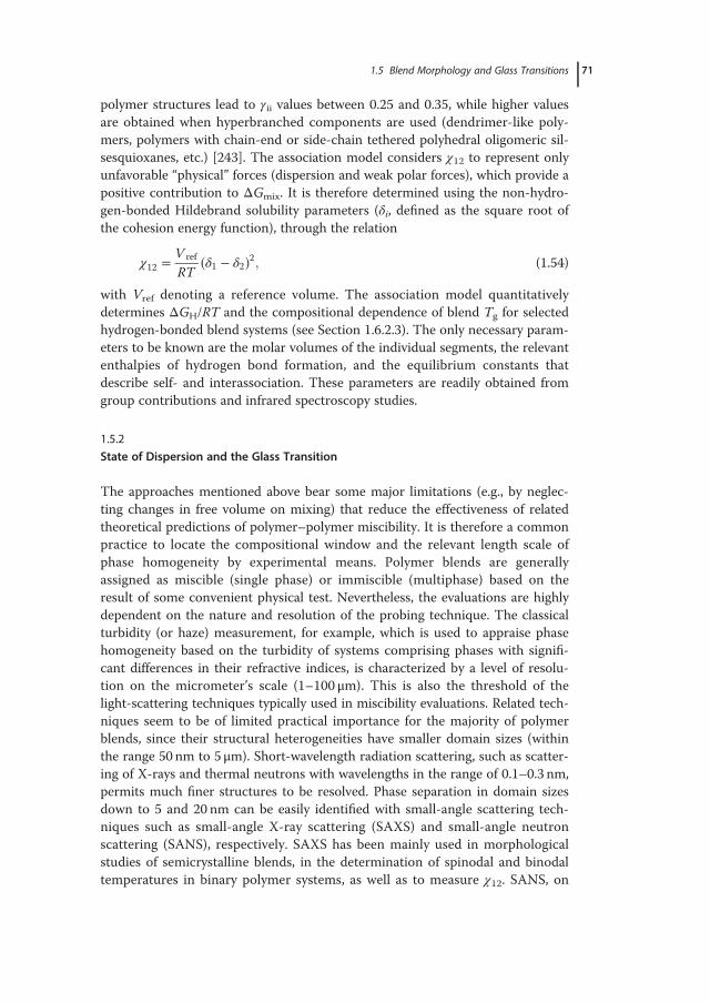
polymer structures lead to γii values between 0.25 and 0.35, while higher valuesare obtained when hyperbranched components are used (dendrimer-like poly-mers, polymers with chain-end or side-chain tethered polyhedral oligomeric sil-sesquioxanes, etc.) [243]. The association model considers χ12 to represent onlyunfavorable “physical” forces (dispersion and weak polar forces), which provide apositive contribution to ΔGmix. It is therefore determined using the non-hydro-gen-bonded Hildebrand solubility parameters (δi, defined as the square root ofthe cohesion energy function), through the relation

χ12 � V ref

RTδ1 � δ2� �2; (1.54)

with Vref denoting a reference volume. The association model quantitativelydetermines ΔGH/RT and the compositional dependence of blend Tg for selectedhydrogen-bonded blend systems (see Section 1.6.2.3). The only necessary param-eters to be known are the molar volumes of the individual segments, the relevantenthalpies of hydrogen bond formation, and the equilibrium constants thatdescribe self- and interassociation. These parameters are readily obtained fromgroup contributions and infrared spectroscopy studies.

1.5.2

State of Dispersion and the Glass Transition

The approaches mentioned above bear some major limitations (e.g., by neglec-ting changes in free volume on mixing) that reduce the effectiveness of relatedtheoretical predictions of polymer–polymer miscibility. It is therefore a commonpractice to locate the compositional window and the relevant length scale ofphase homogeneity by experimental means. Polymer blends are generallyassigned as miscible (single phase) or immiscible (multiphase) based on theresult of some convenient physical test. Nevertheless, the evaluations are highlydependent on the nature and resolution of the probing technique. The classicalturbidity (or haze) measurement, for example, which is used to appraise phasehomogeneity based on the turbidity of systems comprising phases with signifi-cant differences in their refractive indices, is characterized by a level of resolu-tion on the micrometer’s scale (1–100 μm). This is also the threshold of thelight-scattering techniques typically used in miscibility evaluations. Related tech-niques seem to be of limited practical importance for the majority of polymerblends, since their structural heterogeneities have smaller domain sizes (withinthe range 50 nm to 5 μm). Short-wavelength radiation scattering, such as scatter-ing of X-rays and thermal neutrons with wavelengths in the range of 0.1–0.3 nm,permits much finer structures to be resolved. Phase separation in domain sizesdown to 5 and 20 nm can be easily identified with small-angle scattering tech-niques such as small-angle X-ray scattering (SAXS) and small-angle neutronscattering (SANS), respectively. SAXS has been mainly used in morphologicalstudies of semicrystalline blends, in the determination of spinodal and binodaltemperatures in binary polymer systems, as well as to measure χ12. SANS, on


the other hand, has been extensively used to study conformation and morphol-ogy in single- or multicomponent macromolecular systems, in the molten or liq-uid states. Among other molecular spectroscopy techniques, ESR spectroscopyand solid-state NMR measurements of the spin-lattice relaxation times are capa-ble of distinguishing motional traces and structural or dynamic heterogeneitiesat domain sizes down to 2–4 nm. Wide-angle X-ray scattering (WAXS) offersmuch higher resolution, permitting the identification of structural heterogene-ities down to true molecular levels, with scattering phase dimensions in therange 0.1–1 nm. Apparently, the assessment of phase homogeneity by a particu-lar method or technique does not necessarily mean that the assertion is readilyextendible to lower length scales.Without a doubt, glass-transition temperature determinations currently pro-

vide the most popular test for miscibility evaluations. Depending on the chemi-cal nature and the morphology of the system, several DSC studies indicate thatmultiple glass-transition signals are expected to appear at a level of heterogeneitycharacterized by domain sizes within the range of 15–20 nm; contributions fromconsiderably lower domain sizes are detected using thermal techniques of highersensitivity and resolving power (Section 1.4). Still, several complications existthat frequently cast doubt on the interpretation of related results. Problems arisefrom the fact that the glass-transition behavior of any glassy system encompassesthe slowly dissipating memories of its preparation procedure, and the effects ofany special treatment applied to the material prior to testing. The above factors,in combination with potential differences in the rate at which the system hasbeen brought to the conditions of measurement, affect in a usually poorly pre-dictable way its morphological characteristics and preclude direct comparisonsof data obtained for the same material from different laboratories or using differ-ent experimental protocols. In view of that, several studies [2,244] clearly dem-onstrate that a reliable direct relationship between miscibility and the glass-transition phenomenon can be anticipated only in cases where the blend hasachieved its equilibrium morphology before the evaluation, and the behavior ofthe glass-transition signal is unaffected by the experimental method.On the condition that all abovementioned requirements are fulfilled, the num-

ber of transitions and the compositional dependence of the respective glass-tran-sition temperatures offer reliable “indicators” of miscibility, partial miscibility(compatibility), or immiscibility between blend components. Figure 1.26 demon-strates schematically the expected compositional variation of the glass-transitiontemperatures, and the temperature variation of typical dispersion signals indynamic mechanical or dielectric relaxation experiments (see Table 1.3), in eachof these cases. A classic and simple experimental criterion for determining misci-bility is based on the measurement of a single glass-transition signal for all blendcompositions, located in between the glass-transition temperatures of the compo-nents and consistent with the composition of the blend (Figure 1.26a). The singleglass-transition temperature recorded is also frequently referred to as the “blend-average Tg”; its position depends on the type and extent of the interactionsbetween the components, as well as on mixing-induced variations in the free


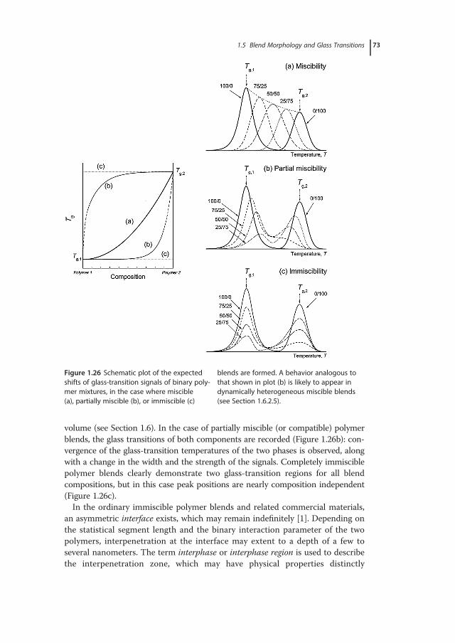
volume (see Section 1.6). In the case of partially miscible (or compatible) polymerblends, the glass transitions of both components are recorded (Figure 1.26b): con-vergence of the glass-transition temperatures of the two phases is observed, alongwith a change in the width and the strength of the signals. Completely immisciblepolymer blends clearly demonstrate two glass-transition regions for all blendcompositions, but in this case peak positions are nearly composition independent(Figure 1.26c).In the ordinary immiscible polymer blends and related commercial materials,

an asymmetric interface exists, which may remain indefinitely [1]. Depending onthe statistical segment length and the binary interaction parameter of the twopolymers, interpenetration at the interface may extent to a depth of a few toseveral nanometers. The term interphase or interphase region is used to describethe interpenetration zone, which may have physical properties distinctly

Figure 1.26 Schematic plot of the expectedshifts of glass-transition signals of binary poly-mer mixtures, in the case where miscible(a), partially miscible (b), or immiscible (c)

blends are formed. A behavior analogous tothat shown in plot (b) is likely to appear indynamically heterogeneous miscible blends(see Section 1.6.2.5).


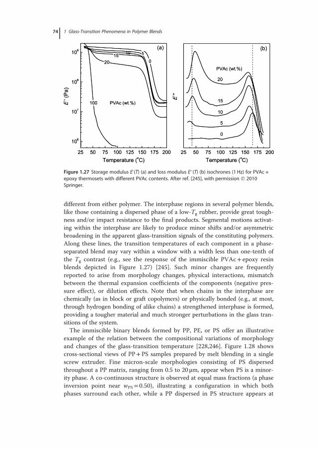
different from either polymer. The interphase regions in several polymer blends,like those containing a dispersed phase of a low-Tg rubber, provide great tough-ness and/or impact resistance to the final products. Segmental motions activat-ing within the interphase are likely to produce minor shifts and/or asymmetricbroadening in the apparent glass-transition signals of the constituting polymers.Along these lines, the transition temperatures of each component in a phase-separated blend may vary within a window with a width less than one-tenth ofthe Tg contrast (e.g., see the response of the immiscible PVAc+ epoxy resinblends depicted in Figure 1.27) [245]. Such minor changes are frequentlyreported to arise from morphology changes, physical interactions, mismatchbetween the thermal expansion coefficients of the components (negative pres-sure effect), or dilution effects. Note that when chains in the interphase arechemically (as in block or graft copolymers) or physically bonded (e.g., at most,through hydrogen bonding of alike chains) a strengthened interphase is formed,providing a tougher material and much stronger perturbations in the glass tran-sitions of the system.The immiscible binary blends formed by PP, PE, or PS offer an illustrative

example of the relation between the compositional variations of morphologyand changes of the glass-transition temperature [228,246]. Figure 1.28 showscross-sectional views of PP+PS samples prepared by melt blending in a singlescrew extruder. Fine micron-scale morphologies consisting of PS dispersedthroughout a PP matrix, ranging from 0.5 to 20 μm, appear when PS is a minor-ity phase. A co-continuous structure is observed at equal mass fractions (a phaseinversion point near wPS= 0.50), illustrating a configuration in which bothphases surround each other, while a PP dispersed in PS structure appears at

Figure 1.27 Storage modulus E´(T) (a) and loss modulus E´´(T) (b) isochrones (1 Hz) for PVAc+epoxy thermosets with different PVAc contents. After ref. [245], with permission 2010Springer.


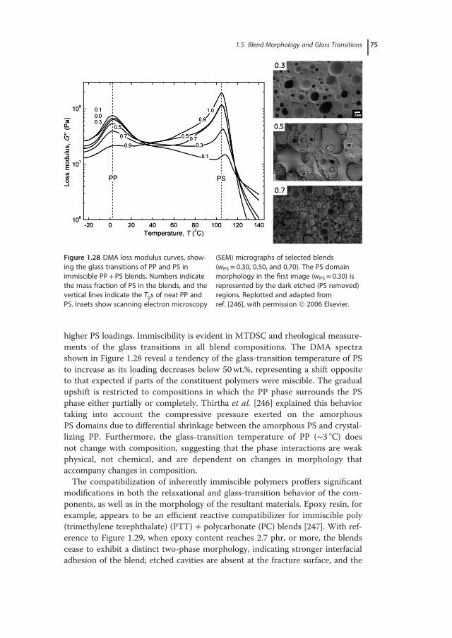
higher PS loadings. Immiscibility is evident in MTDSC and rheological measure-ments of the glass transitions in all blend compositions. The DMA spectrashown in Figure 1.28 reveal a tendency of the glass-transition temperature of PSto increase as its loading decreases below 50wt.%, representing a shift oppositeto that expected if parts of the constituent polymers were miscible. The gradualupshift is restricted to compositions in which the PP phase surrounds the PSphase either partially or completely. Thirtha et al. [246] explained this behaviortaking into account the compressive pressure exerted on the amorphousPS domains due to differential shrinkage between the amorphous PS and crystal-lizing PP. Furthermore, the glass-transition temperature of PP (∼3 °C) doesnot change with composition, suggesting that the phase interactions are weakphysical, not chemical, and are dependent on changes in morphology thataccompany changes in composition.The compatibilization of inherently immiscible polymers proffers significant

modifications in both the relaxational and glass-transition behavior of the com-ponents, as well as in the morphology of the resultant materials. Epoxy resin, forexample, appears to be an efficient reactive compatibilizer for immiscible poly(trimethylene terephthalate) (PTT) + polycarbonate (PC) blends [247]. With ref-erence to Figure 1.29, when epoxy content reaches 2.7 phr, or more, the blendscease to exhibit a distinct two-phase morphology, indicating stronger interfacialadhesion of the blend; etched cavities are absent at the fracture surface, and the

Figure 1.28 DMA loss modulus curves, show-ing the glass transitions of PP and PS inimmiscible PP+ PS blends. Numbers indicatethe mass fraction of PS in the blends, and thevertical lines indicate the Tgs of neat PP andPS. Insets show scanning electron microscopy

(SEM) micrographs of selected blends(wPS= 0.30, 0.50, and 0.70). The PS domainmorphology in the first image (wPS= 0.30) isrepresented by the dark etched (PS removed)regions. Replotted and adapted fromref. [246], with permission 2006 Elsevier.


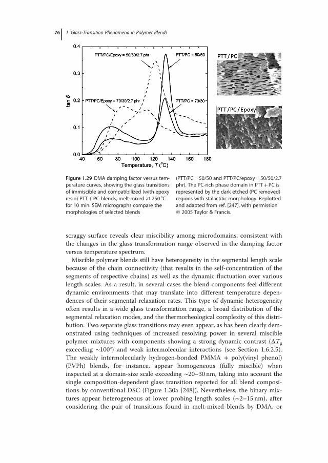
scraggy surface reveals clear miscibility among microdomains, consistent withthe changes in the glass transformation range observed in the damping factorversus temperature spectrum.Miscible polymer blends still have heterogeneity in the segmental length scale

because of the chain connectivity (that results in the self-concentration of thesegments of respective chains) as well as the dynamic fluctuation over variouslength scales. As a result, in several cases the blend components feel differentdynamic environments that may translate into different temperature depen-dences of their segmental relaxation rates. This type of dynamic heterogeneityoften results in a wide glass transformation range, a broad distribution of thesegmental relaxation modes, and the thermorheological complexity of this distri-bution. Two separate glass transitions may even appear, as has been clearly dem-onstrated using techniques of increased resolving power in several misciblepolymer mixtures with components showing a strong dynamic contrast (ΔTg

exceeding ∼100°) and weak intermolecular interactions (see Section 1.6.2.5).The weakly intermolecularly hydrogen-bonded PMMA + poly(vinyl phenol)(PVPh) blends, for instance, appear homogeneous (fully miscible) wheninspected at a domain-size scale exceeding ∼20–30 nm, taking into account thesingle composition-dependent glass transition reported for all blend composi-tions by conventional DSC (Figure 1.30a [248]). Nevertheless, the binary mix-tures appear heterogeneous at lower probing length scales (∼2–15 nm), afterconsidering the pair of transitions found in melt-mixed blends by DMA, or

Figure 1.29 DMA damping factor versus tem-perature curves, showing the glass transitionsof immiscible and compatibilized (with epoxyresin) PTT+ PC blends, melt-mixed at 250 °Cfor 10 min. SEM micrographs compare themorphologies of selected blends

(PTT/PC= 50/50 and PTT/PC/epoxy= 50/50/2.7phr). The PC-rich phase domain in PTT+ PC isrepresented by the dark etched (PC removed)regions with stalactitic morphology. Replottedand adapted from ref. [247], with permission 2005 Taylor & Francis.


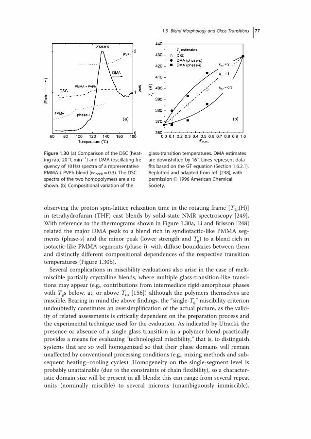
observing the proton spin-lattice relaxation time in the rotating frame [T1ρ(H)]in tetrahydrofuran (THF) cast blends by solid-state NMR spectroscopy [249].With reference to the thermograms shown in Figure 1.30a, Li and Brisson [248]related the major DMA peak to a blend rich in syndiotactic-like PMMA seg-ments (phase-s) and the minor peak (lower strength and Tg) to a blend rich inisotactic-like PMMA segments (phase-i), with diffuse boundaries between themand distinctly different compositional dependences of the respective transitiontemperatures (Figure 1.30b).Several complications in miscibility evaluations also arise in the case of melt-

miscible partially crystalline blends, where multiple glass-transition-like transi-tions may appear (e.g., contributions from intermediate rigid-amorphous phaseswith Tgs below, at, or above Tm [156]) although the polymers themselves aremiscible. Bearing in mind the above findings, the “single-Tg” miscibility criterionundoubtedly constitutes an oversimplification of the actual picture, as the valid-ity of related assessments is critically dependent on the preparation process andthe experimental technique used for the evaluation. As indicated by Utracki, thepresence or absence of a single glass transition in a polymer blend practicallyprovides a means for evaluating “technological miscibility,” that is, to distinguishsystems that are so well homogenized so that their phase domains will remainunaffected by conventional processing conditions (e.g., mixing methods and sub-sequent heating–cooling cycles). Homogeneity on the single-segment level isprobably unattainable (due to the constraints of chain flexibility), so a character-istic domain size will be present in all blends; this can range from several repeatunits (nominally miscible) to several microns (unambiguously immiscible).

Figure 1.30 (a) Comparison of the DSC (heat-ing rate 20 °Cmin�1) and DMA (oscillating fre-quency of 10Hz) spectra of a representativePMMA+ PVPh blend (wPVPh= 0.3). The DSCspectra of the two homopolymers are alsoshown. (b) Compositional variation of the

glass-transition temperatures. DMA estimatesare downshifted by 16°. Lines represent datafits based on the GT equation (Section 1.6.2.1).Replotted and adapted from ref. [248], withpermission 1996 American ChemicalSociety.


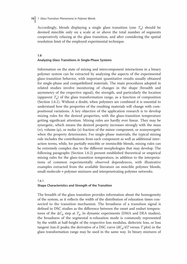
Accordingly, blends displaying a single glass transition (one Tg) should bedeemed miscible only on a scale at or above the total number of segmentscooperatively relaxing at the glass transition, and after considering the spatialresolution limit of the employed experimental technique.

1.6Analyzing Glass Transitions in Single-Phase Systems

Information on the state of mixing and intercomponent interactions in a binarypolymer system can be extracted by analyzing the aspects of the experimentalglass-transition behavior, with important quantitative results usually obtainedfor single-phase and compatibilized materials. The main procedures adopted inrelated studies involve monitoring of changes in the shape (breadth andasymmetry of the respective signal), the strength, and particularly the location(apparent Tg) of the glass transformation range, as a function of composition(Section 1.6.1). Without a doubt, when polymers are combined it is essential tounderstand how the properties of the resulting materials will change with com-positional variations. A key objective of the application research is to developmixing rules for the desired properties, with the glass-transition temperaturegetting significant attention. Mixing rules are hardly ever linear. They may besynergetic, which means the desired property increases strongly with the mass(w), volume (φ), or molar (x) fraction of the minor component, or nonsynergeticwhen the property deteriorates. For single-phase materials, the typical mixingrule includes the contributions from each component as well as additional inter-action terms, while, for partially miscible or immiscible blends, mixing rules canbe extremely complex due to the different morphologies that may develop. Thefollowing paragraphs (Section 1.6.2) present established theoretical or empiricalmixing rules for the glass-transition temperature, in addition to the interpreta-tions of common experimentally observed dependences, with illustrativeexamples extracted from the available literature on miscible polymer blends,small-molecule+ polymer mixtures and interpenetrating polymer networks.

1.6.1

Shape Characteristics and Strength of the Transition

The breadth of the glass transition provides information about the homogeneityof the system, as it reflects the width of the distribution of relaxation times con-nected to the transition mechanism. The broadness of a transition signal isdefined in DSC studies as the difference between the onset and endset tempera-tures of the ΔCp step at Tg. In dynamic experiments (DMA and DEA studies),the broadness of the segmental α-relaxation mode is commonly representedby the width at half-height of the respective loss modulus, dielectric loss, or losstangent (tan δ) peaks; the derivative of a DSC curve (dCp/dT versus T plot) in theglass transformation range may be used in the same way. In binary mixtures of


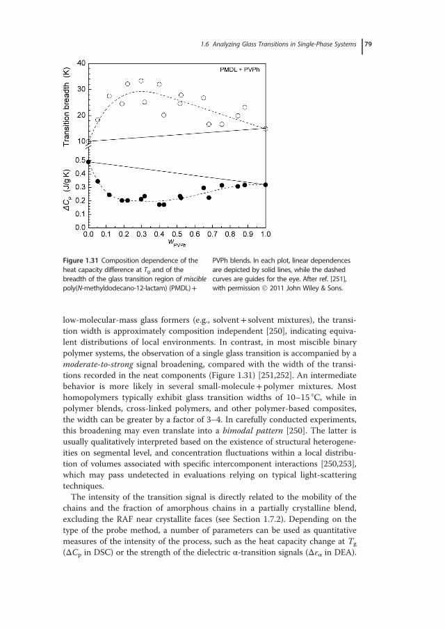
low-molecular-mass glass formers (e.g., solvent+ solvent mixtures), the transi-tion width is approximately composition independent [250], indicating equiva-lent distributions of local environments. In contrast, in most miscible binarypolymer systems, the observation of a single glass transition is accompanied by amoderate-to-strong signal broadening, compared with the width of the transi-tions recorded in the neat components (Figure 1.31) [251,252]. An intermediatebehavior is more likely in several small-molecule+ polymer mixtures. Mosthomopolymers typically exhibit glass transition widths of 10–15 °C, while inpolymer blends, cross-linked polymers, and other polymer-based composites,the width can be greater by a factor of 3–4. In carefully conducted experiments,this broadening may even translate into a bimodal pattern [250]. The latter isusually qualitatively interpreted based on the existence of structural heterogene-ities on segmental level, and concentration fluctuations within a local distribu-tion of volumes associated with specific intercomponent interactions [250,253],which may pass undetected in evaluations relying on typical light-scatteringtechniques.The intensity of the transition signal is directly related to the mobility of the

chains and the fraction of amorphous chains in a partially crystalline blend,excluding the RAF near crystallite faces (see Section 1.7.2). Depending on thetype of the probe method, a number of parameters can be used as quantitativemeasures of the intensity of the process, such as the heat capacity change at Tg

(ΔCp in DSC) or the strength of the dielectric α-transition signals (Δεα in DEA).

Figure 1.31 Composition dependence of theheat capacity difference at Tg and of thebreadth of the glass transition region of misciblepoly(N-methyldodecano-12-lactam) (PMDL)+

PVPh blends. In each plot, linear dependencesare depicted by solid lines, while the dashedcurves are guides for the eye. After ref. [251],with permission 2011 John Wiley & Sons.

1.6 Analyzing Glass Transitions in Single-Phase Systems 79

Early studies indicate that the ΔCp(w) and Tg(w) dependences show a nonlinearand somewhat reversed behavior in blends that exhibit specific interactions (Fig-ure 1.31), while a linear behavior is expected in systems with noninteractingcomponents [254]. Along these lines a decrease in the strength is usually associ-ated with the formation of more ordered structures, with enhanced restrictionsfor the segmental motions occurring within the blend environment, as a result ofintense specific interactions among functional groups along the chains and aconcomitant reduction in free volume.The phase boundary curve of a binary blend can be determined by studying, as

a function of annealing temperature and time, the development of the twophases that form when the miscibility gap is entered [236,255]. The usability oftransition breadths in determining phase behavior is illustrated in Figure 1.32,using the calorimetric analysis of the thermally induced phase separation processoccurring in PS+ tetramethyl bisphenol-A PC blends [238]. Solution-cast sam-ples of the above mixture demonstrate a single-Tg behavior, at all blend compo-sitions. On heating, the blends turn cloudy due to phase separation and theonset temperature of the phase separation can be readily identified by opticalmethods (e.g., light transmission; open circles in the inset of Figure 1.32a), butalso from the glass-transition behavior after heat treatment. The simple experi-mental procedure employed involves heating the blend at a progressivelyincreasing high annealing temperature for a short period of time, followed byrapid cooling (quenching). In that way, the phase structure at the annealingpoint is frozen and the nonequilibrium morphology can be explored by subse-quent study of thermal events. The glass-transition region recorded by DSC may

Figure 1.32 (a) DSC thermograms of a PS+TMPC blend (wPS= 0.50) after annealing at235 °C or 265 °C, below and above, respec-tively, the respective phase separation tem-perature (∼245 °C). The inset shows the phaseseparation temperatures obtained by DSC

(filled circles) and light transmission (open cir-cles). (a) Change of the transition breadth for aPS+ TMPC blend (wPS= 0.60) as a function ofannealing temperature. In all cases, annealingtime was 5min. After ref. [238], with permis-sion 1992 Elsevier.


be either single or bimodal, depending on whether the annealing temperature isbelow or above, respectively, the phase separation temperature. An LCST-typephase boundary can thus be determined by identifying, for each blend composi-tion, the lowest annealing temperature (cloud point) at which the breadth of thecalorimetric glass-transition signal shows a drastic increase (Figure 1.32b). Goodagreement between the experimental pattern obtained by DSC and the predictedspinodal curve is often demonstrated [236].

1.6.2

Description and Interpretation of Tg versus Composition Behaviors

What holds for the glass-transition temperatures generally holds for severalother properties of binary blends. Mechanical properties, resistance to chemicals,radiation, or heat, they all generally plot the same way as the Tg does withrespect to the relative amounts of each polymer in the blend. For that reason, anextensive theoretical and experimental effort has been devoted in attempts toestablish relations for the compositional dependence of the glass-transition tem-perature of amorphous blends. The usability of the ensuing functions is primar-ily judged by their ability to describe real experimental patterns withoutresorting to the use of adjustable parameters. In several purely phenomeno-logical approaches, however, a number of heuristic parameters have been intro-duced to achieve better correlation of models to experimental data, inevitably, atthe expense of their predictive power. In view of that, frequently emerges theneed to provide a posteriori plausible physical meaning to important empiricalparameters, or establish classification schemes for the blend behaviors. Giventhe multiplicity of approaches and the complexity of the ensuing data interpreta-tions, an overview of the origins and the limits of applicability of selected equa-tions will be discussed in some detail in the following sections.

1.6.2.1 Specific Volumes or Flexible Bonds Additivity ModelsMost of the Tg(w) expressions proposed hitherto for binary systems can be rep-resented as variations of the general mathematical form:

T g � w1T g;1 � kw2T g;2

w1 � kw2; (1.55)

with parameter k representing a model-specific constant, which is usuallyassumed temperature independent. A relation of this form has been proposed byGordon and Taylor (GT) [256], based on the assumption of volume additivity(i.e., ideal volume of mixing) and the existence of a linear change in volume withtemperature. Their constant, kGT, is given by

kGT � ρ1Δα2=ρ2Δα1;

where ρi represents the densities, and Δαi= (αliquid� αglass)i is the change inexpansivities at the glass transition of the homopolymers. The GT relation wasinitially derived for copolymers, and subsequently extensively used in studies of


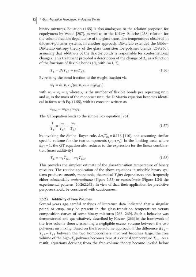
binary mixtures. Equation (1.55) is also analogous to the relation proposed forcopolymers by Wood [257], as well as to the Kelley–Bueche [258] relation forthe volume fraction dependence of the glass-transition temperatures observed indiluent+ polymer systems. In another approach, DiMarzio extended the Gibbs–DiMarzio entropy theory of the glass transition for polymer blends [259,260],assuming that additivity of the flexible bonds is responsible for conformationalchanges. This treatment provided a description of the change of Tg as a functionof the fractions of flexible bonds (Bi, with i= 1, 2),

T g � B1T g;1 � B2T g;2: (1.56)

By relating the bond fraction to the weight fraction via

w1 � m1B1γ1=�m1B1γ2 �m2B2γ1�;with w1 � w2 � 1, where γi is the number of flexible bonds per repeating unit,and mi is the mass of the monomer unit, the DiMarzio equation becomes identi-cal in form with Eq. (1.55), with its constant written as

kDM � m1γ2=m2γ1:

The GT equation leads to the simple Fox equation [261]

1T g

� w1

T g;1� w2

T g;2(1.57)

by invoking the Simha–Boyer rule, ΔαiTg,i= 0.113 [110], and assuming similarspecific volume for the two components (ρ1� ρ2). In the limiting case, wherekGT= 1, the GT equation also reduces to the expression for the linear combina-tion (mass additivity)

T g � w1T g;1 � w2T g;2: (1.58)

This provides the simplest estimate of the glass-transition temperature of binarymixtures. The routine application of the above equations in miscible binary sys-tems produces smooth, monotonic, theoretical Tg(w) dependences that frequentlyeither substantially underestimate (Figure 1.33) or overestimate (Figure 1.34) theexperimental patterns [10,262,263]. In view of that, their application for predictivepurposes should be considered with cautiousness.

1.6.2.2 Additivity of Free VolumesSeveral years ago careful analyses of literature data indicated that a singularpoint, or cusp, may be present in the glass-transition temperatures versuscomposition curves of some binary mixtures [266–269]. Such a behavior wasdemonstrated and quantitatively described by Kovacs [266] in the framework ofthe free-volume theory, assuming a negligible excess volume between the twopolymers on mixing. Based on the free-volume approach, if the difference ΔTg=Tg,2�Tg,1 between the two homopolymers involved becomes large, the freevolume of the high-Tg polymer becomes zero at a critical temperature Tcrit. As aresult, equations deriving from the free-volume theory become invalid below


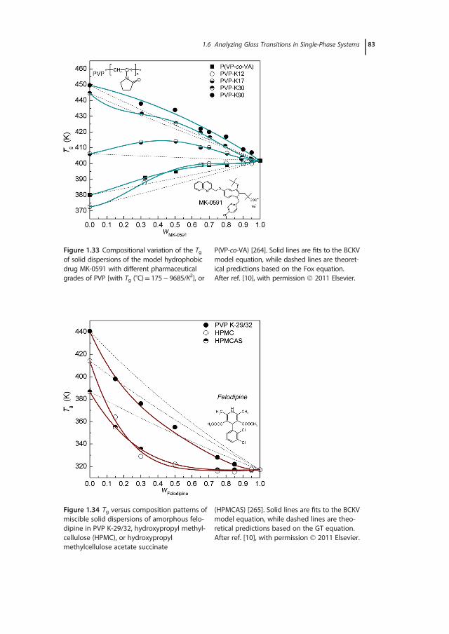
Figure 1.34 Tg versus composition patterns ofmiscible solid dispersions of amorphous felo-dipine in PVP K-29/32, hydroxypropyl methyl-cellulose (HPMC), or hydroxypropylmethylcellulose acetate succinate

(HPMCAS) [265]. Solid lines are fits to the BCKVmodel equation, while dashed lines are theo-retical predictions based on the GT equation.After ref. [10], with permission 2011 Elsevier.

Figure 1.33 Compositional variation of the Tgof solid dispersions of the model hydrophobicdrug MK-0591 with different pharmaceuticalgrades of PVP [with Tg (°C)= 175� 9685/K2], or

P(VP-co-VA) [264]. Solid lines are fits to the BCKVmodel equation, while dashed lines are theoret-ical predictions based on the Fox equation.After ref. [10], with permission 2011 Elsevier.


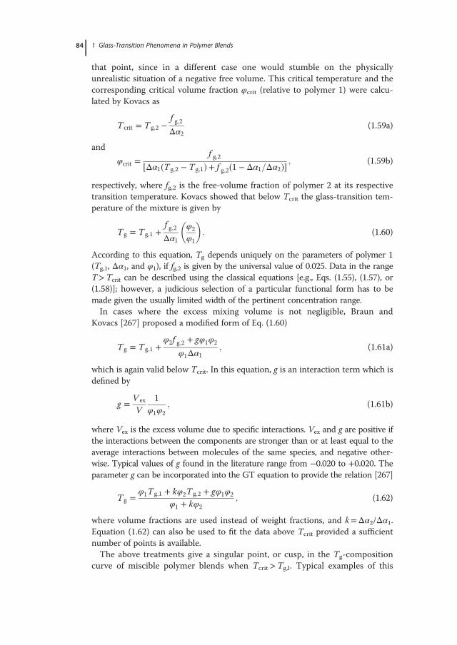
that point, since in a different case one would stumble on the physicallyunrealistic situation of a negative free volume. This critical temperature and thecorresponding critical volume fraction φcrit (relative to polymer 1) were calcu-lated by Kovacs as

T crit � T g;2 � f g;2Δα2

(1.59a)

and

φcrit � f g;2�Δα1�T g;2 � T g;1� � f g;2�1 � Δα1=Δα2�� ; (1.59b)

respectively, where fg,2 is the free-volume fraction of polymer 2 at its respectivetransition temperature. Kovacs showed that below Tcrit the glass-transition tem-perature of the mixture is given by

T g � T g;1 � f g;2Δα1

φ2

φ1

� �: (1.60)

According to this equation, Tg depends uniquely on the parameters of polymer 1(Tg,1, Δα1, and φ1), if fg,2 is given by the universal value of 0.025. Data in the rangeT>Tcrit can be described using the classical equations [e.g., Eqs. (1.55), (1.57), or(1.58)]; however, a judicious selection of a particular functional form has to bemade given the usually limited width of the pertinent concentration range.In cases where the excess mixing volume is not negligible, Braun and

Kovacs [267] proposed a modified form of Eq. (1.60)

T g � T g;1 � φ2f g;2 � gφ1φ2

φ1Δα1; (1.61a)

which is again valid below Tcrit. In this equation, g is an interaction term which isdefined by

g � V ex

V1

φ1φ2; (1.61b)

where Vex is the excess volume due to specific interactions. Vex and g are positive ifthe interactions between the components are stronger than or at least equal to theaverage interactions between molecules of the same species, and negative other-wise. Typical values of g found in the literature range from �0.020 to +0.020. Theparameter g can be incorporated into the GT equation to provide the relation [267]

T g � φ1T g;1 � kφ2T g;2 � gφ1φ2

φ1 � kφ2; (1.62)

where volume fractions are used instead of weight fractions, and k=Δα2/Δα1.Equation (1.62) can also be used to fit the data above Tcrit provided a sufficientnumber of points is available.The above treatments give a singular point, or cusp, in the Tg-composition

curve of miscible polymer blends when Tcrit>Tg,l. Typical examples of this


behavior can be found in blends of poly(ε-caprolactone) (PCL) with several chlo-rinated polymers [267,268] (e.g., chlorinated PVC; Figure 1.35), PVAc with ali-phatic polyesters [270], PEO+PVPh [271], PVME+PVPh [271,272], poly(vinylethyl ether) (PVEE)+PVPh [273], and several other binary mixtures[269,270,274]. As a rule of thumb, Aubin and Prud’homme [268] indicate that acusp is likely to appear if the difference ΔTg is greater than 52 K, in practicehigher than at least 70°–80°, and Δα2 is sufficiently large.

1.6.2.3 Predictions Based on Thermodynamic ConsiderationsCouchman and Karasz [275] and Couchman [276,277] followed a classical ther-modynamic treatment of the glass transition that provided several relations forthe compositional dependence of the apparent glass-transition temperature invarious single-phased solid solutions. The approach is based on the suppositionof continuity of the thermodynamic entropy [275] or enthalpy [276] functions atTg, and equality of the respective excess functions of mixing of the liquid (melt)and glass states. In the entropy model used by Couchman and Karasz, the com-ponents of a miscible binary polymer blend were considered to have pure-com-ponent molar entropies denoted as S1 and S2, and respective mole fractions x1and x2. The molar entropy of the mixed system is expressed as

S � x1S1 � x2S2 � ΔSmix; (1.63)

Figure 1.35 Glass-transition temperature ofPCL + chlorinated PVC (CPVC) blends as afunction of volume fraction, φ2, of CPVC in theamorphous phase (data from ref. [268], withpermission 1988 John Wiley & Sons). Using

the iso-free-volume theory predictionsof fg,2= 0.025 and Δα2= 0.00 048 K�1, Tcrit isestimated to be Tcrit= Tg,2� 52 K= 336 K andφcrit= 0.28 (relative to polymer 1).


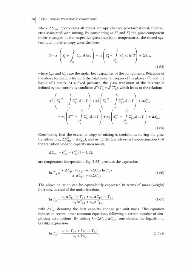
where ΔSmix incorporates all excess entropy changes (conformational, thermal,etc.) associated with mixing. By considering as So1 and So2 the pure-componentmolar entropies at the respective glass-transition temperatures, the mixed sys-tem total molar entropy takes the form

S � x1 So1 �ZTTg;1

Cp;1d ln T

0B@

1CA � x2 So2 �

ZTTg;2

Cp;2d ln T

0B@

1CA � ΔSmix;

(1.64)

where Cp,l and Cp,2 are the molar heat capacities of the components. Relations ofthe above form apply for both the total molar entropies of the glassy (SG) and theliquid (SL) states. At a fixed pressure, the glass transition of the mixture isdefined by the continuity condition SG(Tg)= SL(Tg), which leads to the relation:

xG1 So;G1 �ZTg

Tg;1

CGp;1d ln T

0B@

1CA � xG2 So;G2 �

ZTg

T g;2

CGp;2d ln T

0B@

1CA � ΔSGmix

� xL1 So;L1 �ZTg

Tg;1

CLp;1d ln T

0B@

1CA � xL2 So;L2 �

ZTg

Tg;2

CLp;2d ln T

0B@

1CA � ΔSLmix

:

(1.65)

Considering that the excess entropy of mixing is continuous during the glasstransition (i.e., ΔSGmix � ΔSLmix), and using the (zeroth order) approximation thatthe transition isobaric capacity increments,

ΔCp;i � CLp;i � CG

p;i �i � 1; 2�;are temperature independent, Eq. (1.65) provides the expression

ln T g � x1ΔCp;1 ln T g;1 � x2ΔCp;2 ln T g;2

x1ΔCp;1 � x2ΔCp;2: (1.66)

The above equation can be equivalently expressed in terms of mass (weight)fractions, instead of the molar fractions,

ln T g � w1ΔCp;1 ln T g;1 � w2ΔCp;2 ln T g;2

w1ΔCp;1 � w2ΔCp;2; (1.67)

with ΔCp,i denoting the heat capacity change per unit mass. This equationreduces to several other common equations, following a certain number of sim-plifying assumptions. By setting k=ΔCp,2/ΔCp,1, one obtains the logarithmicGT-like expression

ln T g � w1 ln T g;1 � kw2 ln T g;2

w1 � kw2; (1.68a)


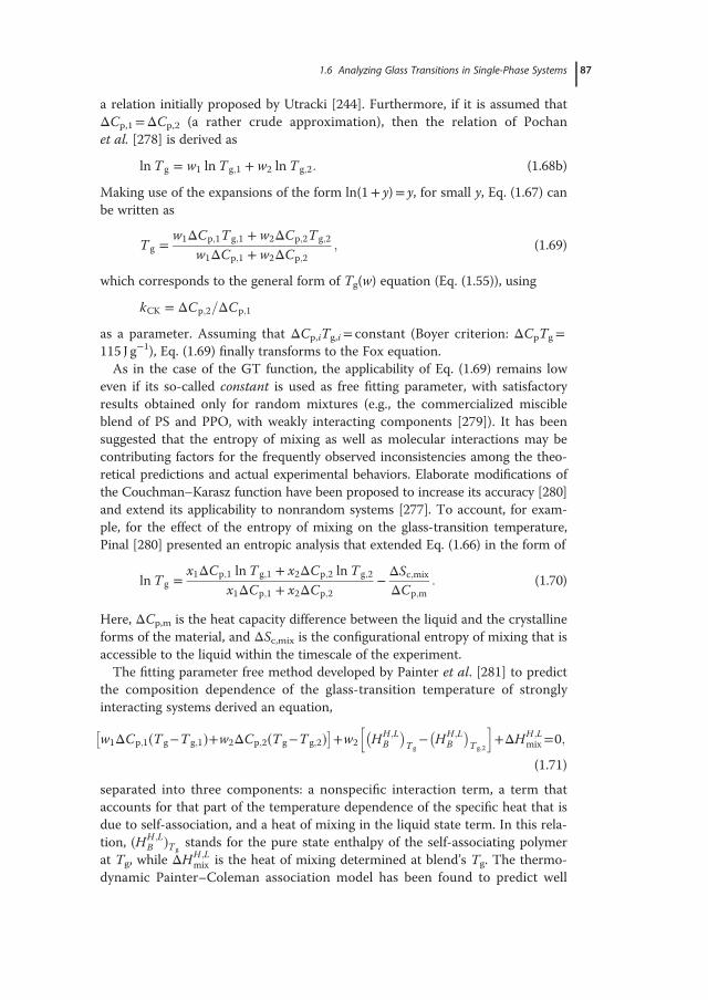
a relation initially proposed by Utracki [244]. Furthermore, if it is assumed thatΔCp,1=ΔCp,2 (a rather crude approximation), then the relation of Pochanet al. [278] is derived as

ln T g � w1 ln T g;1 � w2 ln T g;2: (1.68b)

Making use of the expansions of the form ln(1+ y)= y, for small y, Eq. (1.67) canbe written as

T g � w1ΔCp;1T g;1 � w2ΔCp;2T g;2

w1ΔCp;1 � w2ΔCp;2; (1.69)

which corresponds to the general form of Tg(w) equation (Eq. (1.55)), using

kCK � ΔCp;2=ΔCp;1

as a parameter. Assuming that ΔCp,iTg,i= constant (Boyer criterion: ΔCpTg=115 J g�1), Eq. (1.69) finally transforms to the Fox equation.As in the case of the GT function, the applicability of Eq. (1.69) remains low

even if its so-called constant is used as free fitting parameter, with satisfactoryresults obtained only for random mixtures (e.g., the commercialized miscibleblend of PS and PPO, with weakly interacting components [279]). It has beensuggested that the entropy of mixing as well as molecular interactions may becontributing factors for the frequently observed inconsistencies among the theo-retical predictions and actual experimental behaviors. Elaborate modifications ofthe Couchman–Karasz function have been proposed to increase its accuracy [280]and extend its applicability to nonrandom systems [277]. To account, for exam-ple, for the effect of the entropy of mixing on the glass-transition temperature,Pinal [280] presented an entropic analysis that extended Eq. (1.66) in the form of

ln T g � x1ΔCp;1 lnT g;1 � x2ΔCp;2 ln T g;2

x1ΔCp;1 � x2ΔCp;2� ΔSc;mix

ΔCp;m: (1.70)

Here, ΔCp,m is the heat capacity difference between the liquid and the crystallineforms of the material, and ΔSc,mix is the configurational entropy of mixing that isaccessible to the liquid within the timescale of the experiment.The fitting parameter free method developed by Painter et al. [281] to predict

the composition dependence of the glass-transition temperature of stronglyinteracting systems derived an equation,

w1ΔCp;1�T g�T g;1��w2ΔCp;2�T g�T g;2�� w2 HH ;LB

� �Tg� HH;L

B

� �Tg;2

h i�ΔHH ;L

mix�0;

(1.71)

separated into three components: a nonspecific interaction term, a term thataccounts for that part of the temperature dependence of the specific heat that isdue to self-association, and a heat of mixing in the liquid state term. In this rela-tion, �HH ;L

B �Tgstands for the pure state enthalpy of the self-associating polymer

at Tg, while ΔHH ;Lmix is the heat of mixing determined at blend’s Tg. The thermo-

dynamic Painter–Coleman association model has been found to predict well


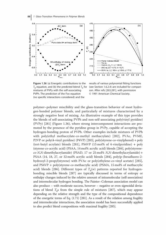
polymer–polymer miscibility and the glass-transition behavior of most hydro-gen-bonded polymer blends, and particularly of mixtures characterized by astrongly negative heat of mixing. An illustrative example of this type providesthe blends of self-associating PVPh and non-self-associating poly(vinyl pyridine)(PVPy) [281] (Figure 1.36), where strong intercomponent interactions are pro-moted by the presence of the pyridine group in PVPy, capable of accepting thehydrogen-bonding proton of PVPh. Other examples include mixtures of PVPhwith poly(ethyl methacrylate-co-methyl methacrylate) [282], PVAc, PVME,P2VP or poly(4-vinyl pyridine) (P4VP) [283], poly(styrene-co-vinylphenol)+ poly(tert-butyl acrylate) blends [281], PS4VP (15mol% of 4-vinylpyridine) + poly(styrene-co-acrylic acid) (PSAA, 14mol% acrylic acid) blends [284], poly(styrene-co-N,N-dimethylacrylamide) (PSAD, 17 or 25mol% N,N-dimethylacrylamide)+PSAA (14, 18, 27, or 32mol% acrylic acid) blends [284], poly(p-(hexafluoro-2-hydroxyl-2-propyl)styrene) with PVAc or poly(ethylene-co-vinyl acetate) [285],and PS4VP + poly(styrene-co-methacrylic acid) (PSMA, 15mol% of methacrylicacid) blends [286]. Different types of Tg(w) patterns reported for hydrogen-bonding miscible blends [287] are typically discussed in terms of entropy orenthalpy changes induced by the relative amount of intramolecular (self-association)and intermolecular hydrogen bonding. The Painter–Coleman association model canalso produce – with moderate success, however – negative or even sigmoidal devia-tions of blend Tgs from the simple rule of mixtures [287], which may appeardepending on the relative strength and the type of the compositional dependenceof the energetic terms of Eq. (1.71) [281]. As a result of the relation among fragilityand intermolecular interactions, the association model has been successfully appliedto also predict blend compositions with maximal fragility [285].

Figure 1.36 (a) Energetic contributions to theTg equation, and (b) the predicted blend Tg formixtures of PVPy with the self-associatingPVPh. The prediction of the Fox equation(no specific interactions considered) and the

results of various polynomial fitting functions(see Section 1.6.2.4) are included for compari-son. After refs [263,281], with permission 1991 American Chemical Society.


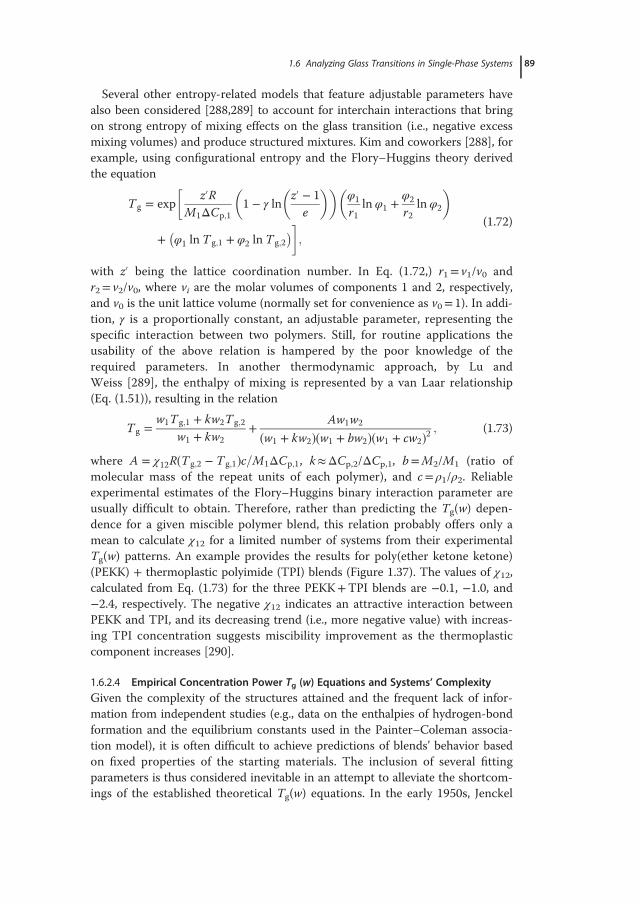
Several other entropy-related models that feature adjustable parameters havealso been considered [288,289] to account for interchain interactions that bringon strong entropy of mixing effects on the glass transition (i.e., negative excessmixing volumes) and produce structured mixtures. Kim and coworkers [288], forexample, using configurational entropy and the Flory–Huggins theory derivedthe equation

T g � exp

z´R

M1ΔCp;11 � γ ln

z´ � 1e

� �� φ1

r1ln φ1 � φ2

r2ln φ2

� �

� φ1 ln T g;1 � φ2 ln T g;2� �

;

(1.72)

with z´ being the lattice coordination number. In Eq. (1.72,) r1= v1/v0 andr2= v2/v0, where vi are the molar volumes of components 1 and 2, respectively,and v0 is the unit lattice volume (normally set for convenience as v0= 1). In addi-tion, γ is a proportionally constant, an adjustable parameter, representing thespecific interaction between two polymers. Still, for routine applications theusability of the above relation is hampered by the poor knowledge of therequired parameters. In another thermodynamic approach, by Lu andWeiss [289], the enthalpy of mixing is represented by a van Laar relationship(Eq. (1.51)), resulting in the relation

T g � w1T g;1 � kw2T g;2

w1 � kw2� Aw1w2

�w1 � kw2��w1 � bw2��w1 � cw2�2 ; (1.73)

where A � χ12R�T g;2 � T g;1�c=M1ΔCp;1, k�ΔCp,2/ΔCp,1, b=M2/M1 (ratio ofmolecular mass of the repeat units of each polymer), and c= ρ1/ρ2. Reliableexperimental estimates of the Flory–Huggins binary interaction parameter areusually difficult to obtain. Therefore, rather than predicting the Tg(w) depen-dence for a given miscible polymer blend, this relation probably offers only amean to calculate χ12 for a limited number of systems from their experimentalTg(w) patterns. An example provides the results for poly(ether ketone ketone)(PEKK) + thermoplastic polyimide (TPI) blends (Figure 1.37). The values of χ12,calculated from Eq. (1.73) for the three PEKK+TPI blends are �0.1, �1.0, and�2.4, respectively. The negative χ12 indicates an attractive interaction betweenPEKK and TPI, and its decreasing trend (i.e., more negative value) with increas-ing TPI concentration suggests miscibility improvement as the thermoplasticcomponent increases [290].

1.6.2.4 Empirical Concentration Power Tg (w) Equations and Systems’ ComplexityGiven the complexity of the structures attained and the frequent lack of infor-mation from independent studies (e.g., data on the enthalpies of hydrogen-bondformation and the equilibrium constants used in the Painter–Coleman associa-tion model), it is often difficult to achieve predictions of blends’ behavior basedon fixed properties of the starting materials. The inclusion of several fittingparameters is thus considered inevitable in an attempt to alleviate the shortcom-ings of the established theoretical Tg(w) equations. In the early 1950s, Jenckel


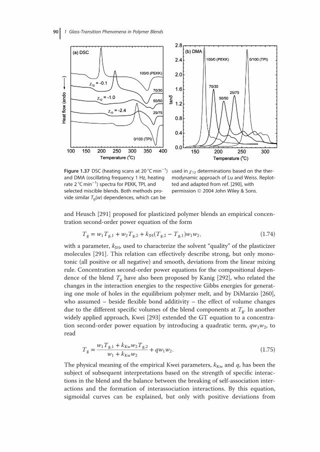
and Heusch [291] proposed for plasticized polymer blends an empirical concen-tration second-order power equation of the form

T g � w1T g;1 � w2T g;2 � kJH�T g;2 � T g;1�w1w2; (1.74)

with a parameter, kJH, used to characterize the solvent “quality” of the plasticizermolecules [291]. This relation can effectively describe strong, but only mono-tonic (all positive or all negative) and smooth, deviations from the linear mixingrule. Concentration second-order power equations for the compositional depen-dence of the blend Tg have also been proposed by Kanig [292], who related thechanges in the interaction energies to the respective Gibbs energies for generat-ing one mole of holes in the equilibrium polymer melt, and by DiMarzio [260],who assumed – beside flexible bond additivity – the effect of volume changesdue to the different specific volumes of the blend components at Tg. In anotherwidely applied approach, Kwei [293] extended the GT equation to a concentra-tion second-order power equation by introducing a quadratic term, qw1w2, toread

T g � w1T g;1 � kKww2T g;2

w1 � kKww2� qw1w2: (1.75)

The physical meaning of the empirical Kwei parameters, kKw and q, has been thesubject of subsequent interpretations based on the strength of specific interac-tions in the blend and the balance between the breaking of self-association inter-actions and the formation of interassociation interactions. By this equation,sigmoidal curves can be explained, but only with positive deviations from

Figure 1.37 DSC (heating scans at 20 °Cmin�1)and DMA (oscillating frequency 1 Hz, heatingrate 2 °Cmin�1) spectra for PEKK, TPI, andselected miscible blends. Both methods pro-vide similar Tg(w) dependences, which can be

used in χ12 determinations based on the ther-modynamic approach of Lu and Weiss. Replot-ted and adapted from ref. [290], withpermission 2004 John Wiley & Sons.


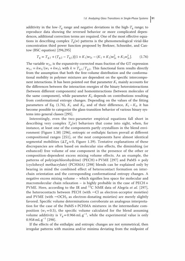
additivity in the low-Tg range and negative deviations in the high-Tg range; toreproduce data showing the reversed behavior or more complicated depen-dences, additional correction terms are required. One of the most effective equa-tions in describing complex Tg(w) patterns is the phenomenological virial-likeconcentration third power function proposed by Brekner, Schneider, and Can-tow (BSC equation) [294,295]

T g � T g;1 � �T g;2 � T g;1��1 � K1�w2c � �K1 � K2�w22c � K2w

32c�: (1.76)

The variable w2,c is the expansivity-corrected mass fraction of the GT expressionw2;c � kw2=�w1 � kw2�, with k � T g;1=T g;2. This functional form results directlyfrom the assumption that both the free-volume distribution and the conforma-tional mobility in polymer mixtures are dependent on the specific intercompo-nent interactions. It has been pointed out that parameter K1 mainly accounts forthe differences between the interaction energies of the binary heterointeractions(between different components) and homointeractions (between molecules ofthe same component), while parameter K2 depends on contributions resultingfrom conformational entropy changes. Depending on the values of the fittingparameters of Eq. (1.76), K1 and K2, and of their difference, K1�K2, it hasbecome possible to categorize the glass-transition behavior of various binary sys-tems into general classes [295].Interestingly, even the two-parameter empirical equations fall short in

describing very complex Tg(w) behaviors that come into sight, when, forinstance, at least one of the components partly crystallizes in the blend envi-ronment (Figure 1.38) [296], entropic or enthalpic factors prevail at differentcompositional ranges [251], or the neat components have almost identicalsegmental mobilities (ΔTg� 0, Figure 1.39). Tentative explanations of thesediscrepancies are often based on molecular size effects, the diminishing (orenhanced) free volume of one component in the presence of the other orcomposition-dependent excess mixing volume effects. As an example, thepatterns of poly(epichlorohydrine) (PECH)+PVME [297] and PαMS + poly(cyclohexyl methacrylate) (PCHMA) [298] blends can be explained only bybearing in mind the combined effect of heterocontact formation on inter-chain orientation and the corresponding conformational entropy changes. Anegative excess mixing volume – which signifies less space for molecular andmacromolecular chain relaxation – is highly probable in the case of PECH+PVME. Here, according to the IR and 13C NMR data of Alegría et al. [297],the heterocontacts between PECH (with ��Cl as electron-acceptor moieties)and PVME (with ��OCH3 as electron-donating moieties) are merely slightlyfavored. Specific volume determinations corroborate an analogous interpreta-tion for the case of the PαMS+PCHMA mixtures: in the intermediate com-position (w1= 0.5), the specific volume calculated for the blend assumingvolume additivity is Vg= 0.966mL g�1, while the experimental value is only0.958mL g�1 [298].If the effects of the enthalpic and entropic changes are not symmetrical, then

irregular patterns with maxima and/or minima deviating from the midpoint of


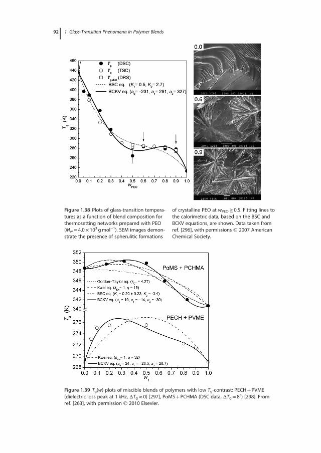
Figure 1.39 Tg(w) plots of miscible blends of polymers with low Tg-contrast: PECH+ PVME(dielectric loss peak at 1 kHz, ΔTg� 0) [297], PαMS+ PCHMA (DSC data, ΔTg= 8°) [298]. Fromref. [263], with permission 2010 Elsevier.

Figure 1.38 Plots of glass-transition tempera-tures as a function of blend composition forthermosetting networks prepared with PEO(Mw= 4.0× 103 gmol�1). SEM images demon-strate the presence of spherulitic formations

of crystalline PEO at wPEO� 0.5. Fitting lines tothe calorimetric data, based on the BSC andBCKV equations, are shown. Data taken fromref. [296], with permissions 2007 AmericanChemical Society.


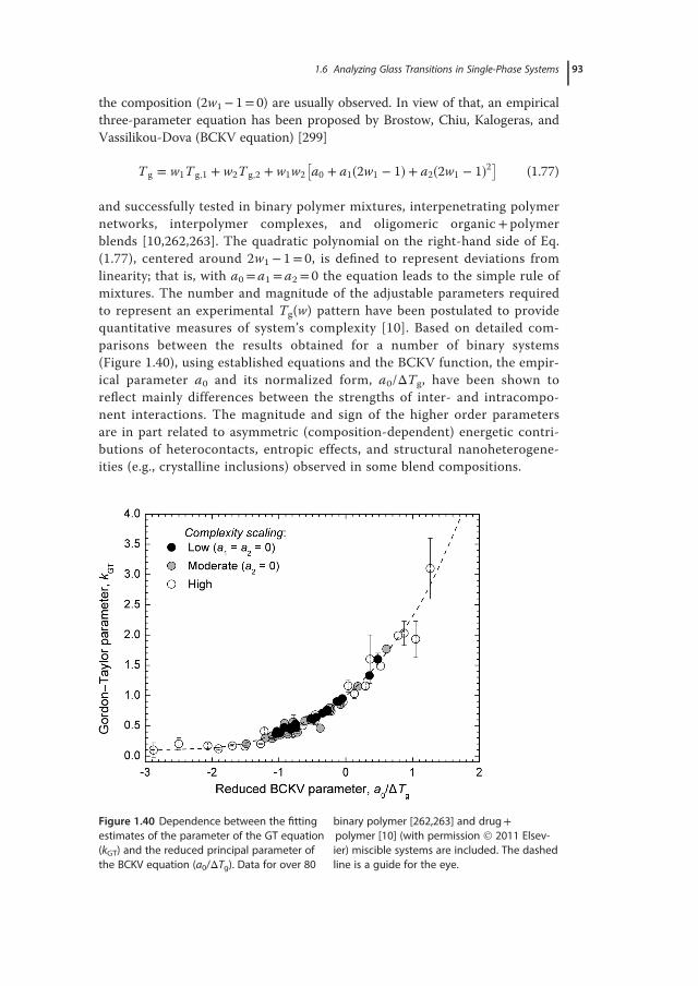
the composition (2w1� 1= 0) are usually observed. In view of that, an empiricalthree-parameter equation has been proposed by Brostow, Chiu, Kalogeras, andVassilikou-Dova (BCKV equation) [299]

T g � w1T g;1 � w2T g;2 � w1w2 a0 � a1�2w1 � 1� � a2�2w1 � 1�2� �(1.77)

and successfully tested in binary polymer mixtures, interpenetrating polymernetworks, interpolymer complexes, and oligomeric organic+ polymerblends [10,262,263]. The quadratic polynomial on the right-hand side of Eq.(1.77), centered around 2w1� 1= 0, is defined to represent deviations fromlinearity; that is, with a0= a1= a2= 0 the equation leads to the simple rule ofmixtures. The number and magnitude of the adjustable parameters requiredto represent an experimental Tg(w) pattern have been postulated to providequantitative measures of system’s complexity [10]. Based on detailed com-parisons between the results obtained for a number of binary systems(Figure 1.40), using established equations and the BCKV function, the empir-ical parameter a0 and its normalized form, a0/ΔTg, have been shown toreflect mainly differences between the strengths of inter- and intracompo-nent interactions. The magnitude and sign of the higher order parametersare in part related to asymmetric (composition-dependent) energetic contri-butions of heterocontacts, entropic effects, and structural nanoheterogene-ities (e.g., crystalline inclusions) observed in some blend compositions.

Figure 1.40 Dependence between the fittingestimates of the parameter of the GT equation(kGT) and the reduced principal parameter ofthe BCKV equation (a0/ΔTg). Data for over 80

binary polymer [262,263] and drug+polymer [10] (with permission 2011 Elsev-ier) miscible systems are included. The dashedline is a guide for the eye.


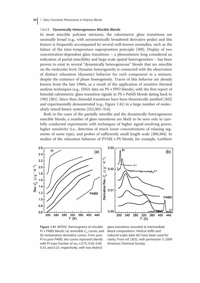
1.6.2.5 Dynamically Heterogeneous Miscible BlendsIn most miscible polymer mixtures, the calorimetric glass transitions areunusually broad (e.g., with asymmetrically broadened derivative peaks) and thisfeature is frequently accompanied by several well-known anomalies, such as thefailure of the time-temperature superposition principle [300]. Display of twoconcentration-dependent glass transitions – a phenomenon long considered anindication of partial miscibility and large-scale spatial heterogeneities – has beenproven to exist in several “dynamically heterogeneous” blends that are miscibleon the molecular level. Dynamic heterogeneity is connected with the observationof distinct relaxation (dynamic) behavior for each component in a mixture,despite the existence of phase homogeneity. Traces of this behavior are alreadyknown from the late 1960s, as a result of the application of sensitive thermalanalysis techniques (e.g., DMA data on PS+PPO blends), with the first report ofbimodal calorimetric glass-transition signals in PS+PαMS blends dating back to1982 [301]. Since then, bimodal transitions have been theoretically justified [302]and experimentally demonstrated (e.g., Figure 1.41) in a large number of molec-ularly mixed binary systems [252,303–314].Both in the cases of the partially miscible and the dynamically heterogeneous

miscible blends, a number of glass transitions are likely to be seen only in care-fully conducted experiments with techniques of higher signal-resolving power,higher sensitivity (i.e., detection of much lower concentrations of relaxing seg-ments of some type), and probes of sufficiently small length scale [300,304]. Instudies of the relaxation behavior of PVME+PS blends, for example, Lorthioir

Figure 1.41 MTDSC thermograms of misciblePI+ P4tBS blends: (a) reversible Cp curves, and(b) temperature derivative curves. From purePI to pure P4tBS, the curves represent blendswith PI mass fraction of wPI= 0.75, 0.50, 0.40,0.33, and 0.25, respectively, with two distinct

glass transitions recorded at intermediateblend compositions. Vertical shifts andreduced scales (plot (b)) have been used forclarity. From ref. [303], with permission 2009American Chemical Society.


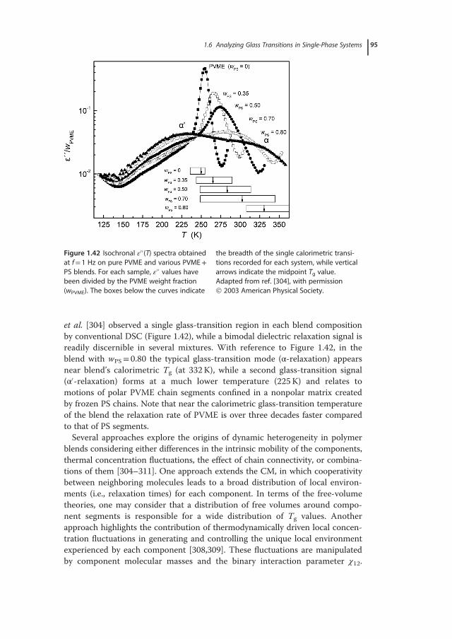
et al. [304] observed a single glass-transition region in each blend compositionby conventional DSC (Figure 1.42), while a bimodal dielectric relaxation signal isreadily discernible in several mixtures. With reference to Figure 1.42, in theblend with wPS= 0.80 the typical glass-transition mode (α-relaxation) appearsnear blend’s calorimetric Tg (at 332 K), while a second glass-transition signal(α´-relaxation) forms at a much lower temperature (225 K) and relates tomotions of polar PVME chain segments confined in a nonpolar matrix createdby frozen PS chains. Note that near the calorimetric glass-transition temperatureof the blend the relaxation rate of PVME is over three decades faster comparedto that of PS segments.Several approaches explore the origins of dynamic heterogeneity in polymer

blends considering either differences in the intrinsic mobility of the components,thermal concentration fluctuations, the effect of chain connectivity, or combina-tions of them [304–311]. One approach extends the CM, in which cooperativitybetween neighboring molecules leads to a broad distribution of local environ-ments (i.e., relaxation times) for each component. In terms of the free-volumetheories, one may consider that a distribution of free volumes around compo-nent segments is responsible for a wide distribution of Tg values. Anotherapproach highlights the contribution of thermodynamically driven local concen-tration fluctuations in generating and controlling the unique local environmentexperienced by each component [308,309]. These fluctuations are manipulatedby component molecular masses and the binary interaction parameter χ12.

Figure 1.42 Isochronal ε´´(T) spectra obtainedat f= 1 Hz on pure PVME and various PVME+PS blends. For each sample, ε´´ values havebeen divided by the PVME weight fraction(wPVME). The boxes below the curves indicate

the breadth of the single calorimetric transi-tions recorded for each system, while verticalarrows indicate the midpoint Tg value.Adapted from ref. [304], with permission 2003 American Physical Society.


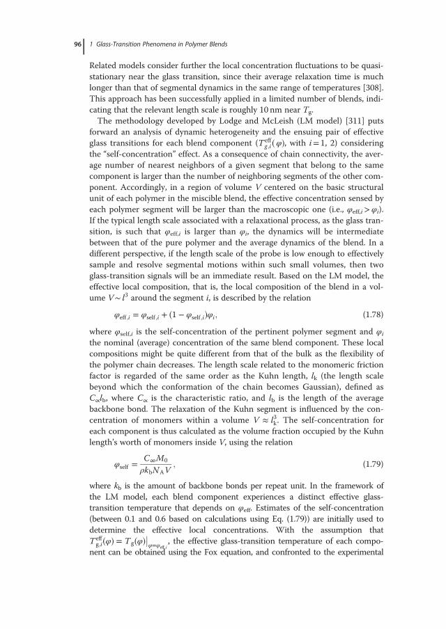
Related models consider further the local concentration fluctuations to be quasi-stationary near the glass transition, since their average relaxation time is muchlonger than that of segmental dynamics in the same range of temperatures [308].This approach has been successfully applied in a limited number of blends, indi-cating that the relevant length scale is roughly 10 nm near Tg.The methodology developed by Lodge and McLeish (LM model) [311] puts

forward an analysis of dynamic heterogeneity and the ensuing pair of effectiveglass transitions for each blend component (T eff

g;i �φ�, with i= 1, 2) consideringthe “self-concentration” effect. As a consequence of chain connectivity, the aver-age number of nearest neighbors of a given segment that belong to the samecomponent is larger than the number of neighboring segments of the other com-ponent. Accordingly, in a region of volume V centered on the basic structuralunit of each polymer in the miscible blend, the effective concentration sensed byeach polymer segment will be larger than the macroscopic one (i.e., φeff,i>φi).If the typical length scale associated with a relaxational process, as the glass tran-sition, is such that φeff,i is larger than φi, the dynamics will be intermediatebetween that of the pure polymer and the average dynamics of the blend. In adifferent perspective, if the length scale of the probe is low enough to effectivelysample and resolve segmental motions within such small volumes, then twoglass-transition signals will be an immediate result. Based on the LM model, theeffective local composition, that is, the local composition of the blend in a vol-ume V∼ l3 around the segment i, is described by the relation

φeff ;i � φself ;i � �1 � φself ;i�φi; (1.78)

where φself,i is the self-concentration of the pertinent polymer segment and φi

the nominal (average) concentration of the same blend component. These localcompositions might be quite different from that of the bulk as the flexibility ofthe polymer chain decreases. The length scale related to the monomeric frictionfactor is regarded of the same order as the Kuhn length, lk (the length scalebeyond which the conformation of the chain becomes Gaussian), defined asC∝lb, where C∝ is the characteristic ratio, and lb is the length of the averagebackbone bond. The relaxation of the Kuhn segment is influenced by the con-centration of monomers within a volume V � l3k. The self-concentration foreach component is thus calculated as the volume fraction occupied by the Kuhnlength’s worth of monomers inside V, using the relation

φself � C1M0

ρkbNAV; (1.79)

where kb is the amount of backbone bonds per repeat unit. In the framework ofthe LM model, each blend component experiences a distinct effective glass-transition temperature that depends on φeff. Estimates of the self-concentration(between 0.1 and 0.6 based on calculations using Eq. (1.79)) are initially used todetermine the effective local concentrations. With the assumption thatT eff

g;i�φ� � T g�φ��φ�φeff ;i, the effective glass-transition temperature of each compo-

nent can be obtained using the Fox equation, and confronted to the experimental


patterns [311–313,315]. Alternatively, the self-concentration can be incorporated asparameter in a suitable Tg,av(φ) or T

effg �φ� equation, to be indirectly obtained by

subsequent fitting of experimental data [262,304–306,312]. In this manner, self-concentration quantifies the extent to which a component has its dynamics per-turbed by the blend partner. The upper limit of φself= 1 denotes a componentshowing its pure or neat component dynamics, while φself= 0 corresponds to acomponent whose dynamics are slaved to those of the blend partner. An exampleof the application of the LM model analysis for miscible PVME + poly(o-chloros-tyrene) (PoCS) blends is shown in Figure 1.43 [306].Several papers provide comparisons of the LM model predictions to either cal-

orimetric data or dynamic results (Table 1.4). The model is generally successfulin predicting component dynamics in athermal polymer blends, though this suc-cess usually relies on using φself as a fitting parameter rather than using its theo-retic estimate. In the case of PI + poly(vinylethylene) (PVE), for example, thetheoretical value of φself,2 is very low to account for the observed behavior [316],suggesting that the self-concentration effect predicted by the LM model is notstrong enough to account for the tracer dynamics of PVE in a PI matrix. Dataevaluations are usually consistent with the model prediction of a smaller self-concentration for the slower component (i.e., φself,1/φself,2> 1), which is expectedto arise from its stiffer backbone and larger Kuhn length (higher persistencelength) [311]. Nevertheless, wide differences often appear between model predic-tions and experimental derivations of the self-concentration. Typically, theoreti-cal predictions are based on the assumption that V � l3k, despite the fact thateven within the assumptions of the LM model a length scale that is of the orderof Kuhn’s length, and not necessarily equal to it, is anticipated. Ample experi-mental evidence suggests that φself, for a given polymer, is matrix dependent,

Figure 1.43 (a) Tg,av (circles) and Tg,1 and Tg,2(squares) of PVME+ PoCS blends againstφPVME. Dashed and dotted curves are Tg,effvalues for the PoCS and PVME components,respectively, calculated by the LM model.

The solid curve is determined by the GTequation with kGT= 0.3. (b) Cp curves. (c)Derivative Cp curves. Tg,1 and Tg,2 are assignedwith arrows [306], with permission 2005American Chemical Society.


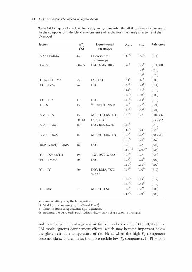
and thus the addition of a geometric factor may be required [300,313,317]. TheLM model ignores confinement effects, which may become important belowthe glass-transition temperature of the blend when the high-Tg componentbecomes glassy and confines the more mobile low-Tg component. In PI + poly

Table 1.4 Examples of miscible binary polymer systems exhibiting distinct segmental dynamicsfor the components in the blend environment and results from their analysis in terms of theLM model.

System ΔTg(°C)

Experimentaltechnique

φself,1 φself,2 Reference

PVAc+PMMA 44 Fluorescencespectroscopy

0.80a) 0.66a) [314]

PI+PVE 60–65 DSC, NMR, DRS 0.45b) 0.25b) [311,318]

0.20b) [319]

0.50a) [320]

PCHA+ PCHMA 75 ESR, DSC 0.21b) 0.41b) [305]

PEO+PVAc 96 DSC 0.26b) 0.23b) [311]

0.64a) 0.16a) [313]

0.40a) 0.08a) [300]

PEO+PLA 110 DSC 0.37a) 0.19a) [313]

PI+PS 130 13C and 2H NMR 0.45b) 0.27b) [321]

0.33a) 0.42a) [321]

PVME+ PS 130 MTDSC, DRS, TSC 0.25c) 0.27 [304,306]

50–130 DEA, DSCd) [239,322]

PVME+ P2CS 150 DSC, DRS, SAXS 0.25b) [240]

0.62a) 0.24a) [323]

PVME+ PoCS 154 MTDSC, DRS, TSC 0.25b) 0.22b) [304,311]

0.15c) 0.20c) [262]

PαMS (5-mer)+PαMS 180 DSC 0.22 0.22 [324]

0.051c) 0.087c) [324]

PCL+PSMAn(14) 190 TSC, DSC, WAXS 0.33b) 0.27 [325]

PEO+PMMA 200 DSC 0.23b) 0.25b) [302]

0.55a) 0.60a) [302]

PCL+PC 206 DSC, DMA, TSC,WAXS

0.33b) 0.05b) [312]

0.47a) 0.19a) [312]

0.20c) 0.49c) [312]

PI+P4tBS 215 MTDSC, DSC 0.45b) 0.2b) [303]

0.63a) 0.03a) [303]

a) Result of fitting using the Fox equation.b) Model prediction using Eq. (1.79) and V � l3k.c) Result of fitting using complex Tg(φ) equations.d) In contrast to DEA, early DSC studies indicate only a single calorimetric signal.


(4-tert-butylstyrene) (P4tBS) [303] and PEO+PMMA [302], for instance, theresults reveal enhanced dynamics for the fast component in a miscible blend attemperatures beneath the glass-transition temperature of the slowest component(nonequilibrium or confinement effect). The model disregards concentrationfluctuations or strong intermolecular interactions, which can influence both themean relaxation time and the breadth of the distribution [300,304].Several instances of borderline miscibility have been reported by examining

the glass-transition behavior of binary systems of very weakly interacting poly-mers, such as PVAc with poly(methyl acrylate) (PMA) [254], PMMA [316], orPEO [313]. Miscibility or immiscibility has been reported for PVAc+PMMAblends, depending on the nature of the solvent [232,316,326], the conditions ofmixing, and the type of thermal treatment [327]. It has been suggested that insolution the conformational changes resulting from hydrogen bond interactionsbetween the two chemically similar polymers and the solvent molecules (chloro-form) may be liable for miscibility [326]. The extremely weak enthalpic interac-tion among PEO and PMMA chains and the slightly negative Flory–Hugginsinteraction parameter are responsible for the marginal miscibility detected forPEO+PMMA blends, based on the single glass-transition temperature followinga Fox-type compositional dependence [328]. The strong dynamic heterogeneityof the system (Table 1.4) is reflected in the complex compositional and tempera-ture dependence of component relaxation times, which indicate that each com-ponent in the blend retains a separate rheological identity [328]. There are, infact, frequent reports of two Tgs and complicated blend morphologies for com-positions with PMMA as a majority component (wPMMA� 0.6) [329]. Strongintermolecular hydrogen bonding, on the other hand, produces a coupling of thesegmental dynamics of the components in blends of polymers with even verylarge intrinsic mobility differences. As a consequence, suppressed dynamic het-erogeneity has been demonstrated in PVME+PVPh (for wPVME� 0.5) [330],PVEE+PVPh (for wPVEE� 0.4) [273,331], and poly(ethyl methacrylate)(PEMA)+PVPh [332] mixtures, while the time-temperature superposition prin-ciple has been reported to hold for PVEE+PVPh, or the strongly interassociatedmixtures of PVPh with P2VP, P4VP, or PVAc [283], for which the Painter–Coleman model is also successfully applied.

1.7Case Studies

1.7.1

Miscibility Achievement via Chemical Modification

In the absence of specific intermolecular interactions, the Gibbs free energy ofmixing is usually positive for polymer blends, due to the small combinatorialentropy of mixing and the positive enthalpy of mixing. Consequently, to exhibitthermodynamic miscibility of the blend, in general, there needs to be some

1.7 Case Studies 99

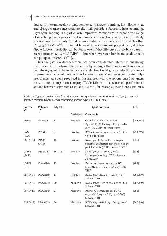
degree of intermolecular interactions (e.g., hydrogen bonding, ion–dipole, π–π,and charge-transfer interactions) that will provide a favorable heat of mixing.Hydrogen bonding is a particularly important mechanism to expand the rangeof miscible polymer pairs since if no favorable interactions are present miscibilityis very rare and is only found when solubility parameters match each other(Δδcrit� 0.1 (MPa)1/2). If favorable weak interactions are present (e.g., dipole–dipole forces), miscibility can be found even if the difference in solubility param-eters approach Δδcrit= 1.0 (MPa)1/2, but when hydrogen bonds are established itcan go up to ∼6.0 (MPa)1/2 [3].Over the past few decades, there has been considerable interest in enhancing

the miscibility of polymer blends, either by adding a third component as a com-patibilizing agent or by introducing specific functional groups into the polymersto promote exothermic interactions between them. Many novel and useful poly-mer blends have been produced in this manner, with the styrene-based polymersconstituting an important category (Table 1.5). In the absence of specific inter-actions between segments of PS and PMMA, for example, their blends exhibit a

Table 1.5 Type of the deviation from the linear mixing rule and description of the Tg (w) patterns inselected miscible binary blends containing styrene-type units (DSC data).

Polymer1a)

Polymer2a)

ΔTg (°C) Tg(w) patterns Ref.

Deviation Comments

PαMS PCHMA 8 Positive Complexity: BSC (K1= 0.20,K2=�3.4), BCKV (α0= 19, α1=�14,α2=�30). Solvent: chloroform

[258,263]

SAN(17.3)

PMMA 8 Positive BCKV (α0= 12, α1=�8, α2= 0). Sol-vent: chloroform

[254,263]

PSCA(15) P4VP(16.6)

13 Positive Kwei (q= 50, kKw= 1). Hydrogenbonding and partial protonation of thepyridine units (FTIR). Solvent: DMF

[337]

PS4VP(5–50)

PSMA(20) 16 . . . 33 Positive Kwei (q= 20 . . . 60, kKw= 1).Hydrogen bonding (FTIR). Solvent:chloroform

[338]

PS4VP(15)

PSAA(14) 15 Positive Painter–Coleman model. BCKV(α0= 21, α1= 5.6, α2= 2.4). Solvent:THF

[284]

PSAD(17) PSAA(18) 17 Positive BCKV (α0= 21.6, α1= 0.1, α2= 17).Solvent: THF

[263,339]

PSAD(17) PSAA(27) 20 Negative BCKV (α0=�4.9, α1= 2.6, α2=�6.2).Solvent: THF

[263,340]

PSAD(25) PSAA(14) 21 Negative Painter-Coleman model. BCKV(α0=�38.8, α1=�6.13, α2= 67.46).Solvent: THF

[284]

PSAD(17) PSAA(32) 26 Negative BCKV (α0=�64.9, α1= 36, α2=�4.5).Solvent: THF

[263,340]


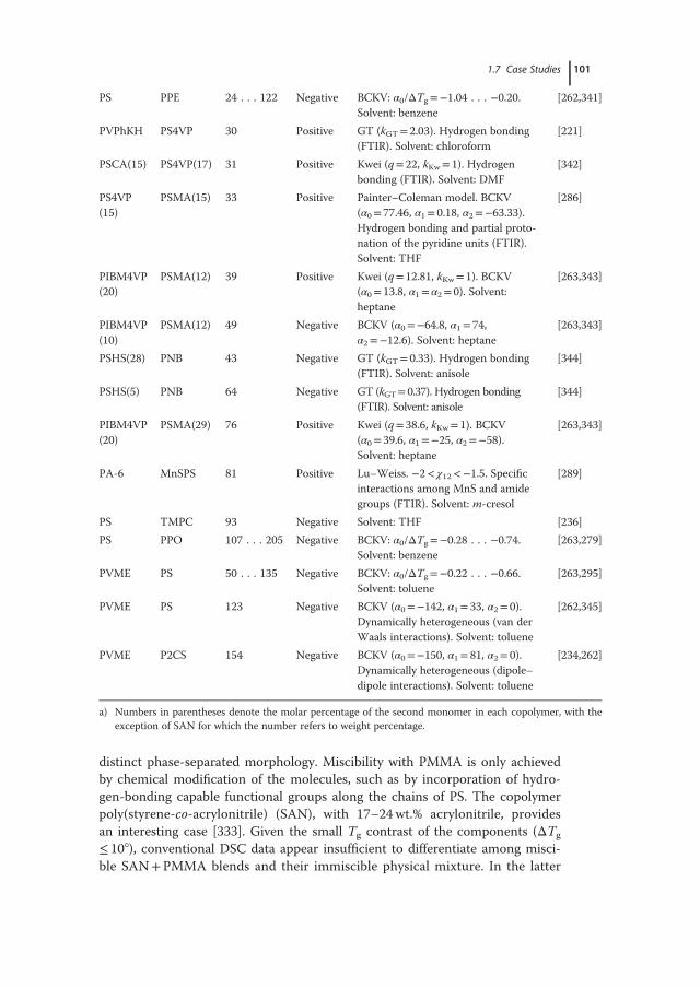
distinct phase-separated morphology. Miscibility with PMMA is only achievedby chemical modification of the molecules, such as by incorporation of hydro-gen-bonding capable functional groups along the chains of PS. The copolymerpoly(styrene-co-acrylonitrile) (SAN), with 17–24wt.% acrylonitrile, providesan interesting case [333]. Given the small Tg contrast of the components (ΔTg

� 10°), conventional DSC data appear insufficient to differentiate among misci-ble SAN+PMMA blends and their immiscible physical mixture. In the latter

PS PPE 24 . . . 122 Negative BCKV: α0/ΔTg=�1.04 . . . �0.20.Solvent: benzene

[262,341]

PVPhKH PS4VP 30 Positive GT (kGT= 2.03). Hydrogen bonding(FTIR). Solvent: chloroform

[221]

PSCA(15) PS4VP(17) 31 Positive Kwei (q= 22, kKw= 1). Hydrogenbonding (FTIR). Solvent: DMF

[342]

PS4VP(15)

PSMA(15) 33 Positive Painter–Coleman model. BCKV(α0= 77.46, α1= 0.18, α2=�63.33).Hydrogen bonding and partial proto-nation of the pyridine units (FTIR).Solvent: THF

[286]

PIBM4VP(20)

PSMA(12) 39 Positive Kwei (q= 12.81, kKw= 1). BCKV(α0= 13.8, α1= α2= 0). Solvent:heptane

[263,343]

PIBM4VP(10)

PSMA(12) 49 Negative BCKV (α0=�64.8, α1= 74,α2=�12.6). Solvent: heptane

[263,343]

PSHS(28) PNB 43 Negative GT (kGT= 0.33). Hydrogen bonding(FTIR). Solvent: anisole

[344]

PSHS(5) PNB 64 Negative GT (kGT= 0.37). Hydrogen bonding(FTIR). Solvent: anisole

[344]

PIBM4VP(20)

PSMA(29) 76 Positive Kwei (q= 38.6, kKw= 1). BCKV(α0= 39.6, α1=�25, α2=�58).Solvent: heptane

[263,343]

PA-6 MnSPS 81 Positive Lu–Weiss. �2< χ12<�1.5. Specificinteractions among MnS and amidegroups (FTIR). Solvent: m-cresol

[289]

PS TMPC 93 Negative Solvent: THF [236]

PS PPO 107 . . . 205 Negative BCKV: α0/ΔTg=�0.28 . . . �0.74.Solvent: benzene

[263,279]

PVME PS 50 . . . 135 Negative BCKV: α0/ΔTg=�0.22 . . . �0.66.Solvent: toluene

[263,295]

PVME PS 123 Negative BCKV (α0=�142, α1= 33, α2= 0).Dynamically heterogeneous (van derWaals interactions). Solvent: toluene

[262,345]

PVME P2CS 154 Negative BCKV (α0=�150, α1= 81, α2= 0).Dynamically heterogeneous (dipole–dipole interactions). Solvent: toluene

[234,262]

a) Numbers in parentheses denote the molar percentage of the second monomer in each copolymer, with theexception of SAN for which the number refers to weight percentage.

1.7 Case Studies 101

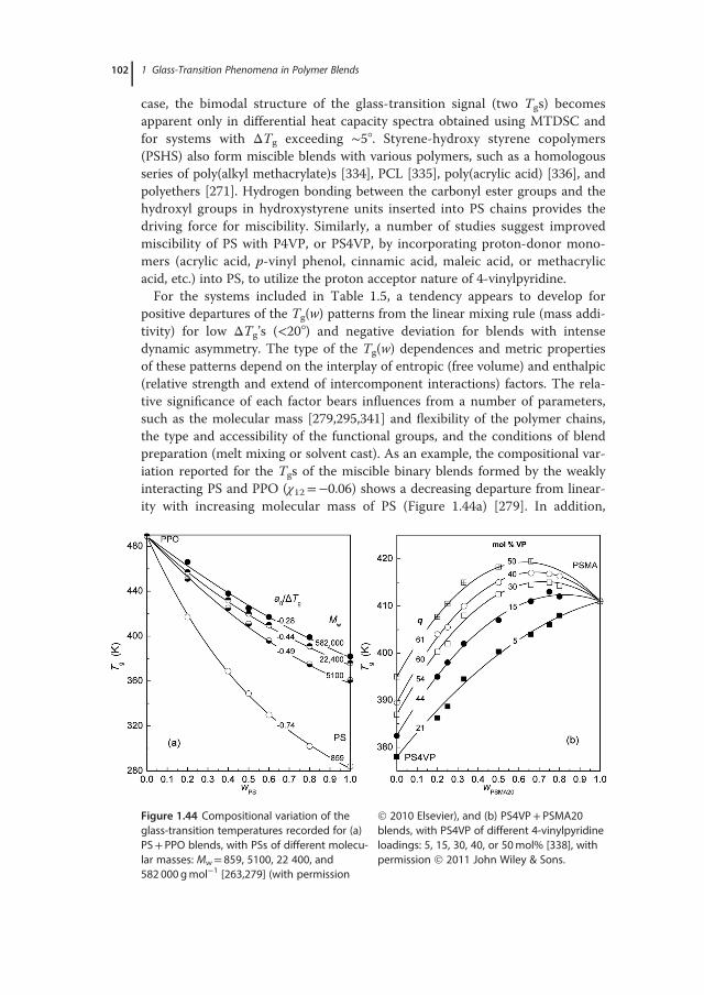
case, the bimodal structure of the glass-transition signal (two Tgs) becomesapparent only in differential heat capacity spectra obtained using MTDSC andfor systems with ΔTg exceeding ∼5°. Styrene-hydroxy styrene copolymers(PSHS) also form miscible blends with various polymers, such as a homologousseries of poly(alkyl methacrylate)s [334], PCL [335], poly(acrylic acid) [336], andpolyethers [271]. Hydrogen bonding between the carbonyl ester groups and thehydroxyl groups in hydroxystyrene units inserted into PS chains provides thedriving force for miscibility. Similarly, a number of studies suggest improvedmiscibility of PS with P4VP, or PS4VP, by incorporating proton-donor mono-mers (acrylic acid, p-vinyl phenol, cinnamic acid, maleic acid, or methacrylicacid, etc.) into PS, to utilize the proton acceptor nature of 4-vinylpyridine.For the systems included in Table 1.5, a tendency appears to develop for

positive departures of the Tg(w) patterns from the linear mixing rule (mass addi-tivity) for low ΔTg’s (<20°) and negative deviation for blends with intensedynamic asymmetry. The type of the Tg(w) dependences and metric propertiesof these patterns depend on the interplay of entropic (free volume) and enthalpic(relative strength and extend of intercomponent interactions) factors. The rela-tive significance of each factor bears influences from a number of parameters,such as the molecular mass [279,295,341] and flexibility of the polymer chains,the type and accessibility of the functional groups, and the conditions of blendpreparation (melt mixing or solvent cast). As an example, the compositional var-iation reported for the Tgs of the miscible binary blends formed by the weaklyinteracting PS and PPO (χ12=�0.06) shows a decreasing departure from linear-ity with increasing molecular mass of PS (Figure 1.44a) [279]. In addition,

Figure 1.44 Compositional variation of theglass-transition temperatures recorded for (a)PS+ PPO blends, with PSs of different molecu-lar masses: Mw= 859, 5100, 22 400, and582 000 gmol�1 [263,279] (with permission

2010 Elsevier), and (b) PS4VP+ PSMA20blends, with PS4VP of different 4-vinylpyridineloadings: 5, 15, 30, 40, or 50mol% [338], withpermission 2011 John Wiley & Sons.


depending on the nature of the interacting species, their densities within thepolymer chains, and the nature of the solvent [344,346], miscible polymerblends, or interpolymer complexes can be prepared [338,342,343]. Benabdel-ghani and Etxeberria [338], for example, reported a gradually intensified eleva-tion of the Tg(w) pattern (Figure 1.44b), accompanied by higher thermal stabilityfor the blends and a stronger intercomponent hydrogen-bonding interaction,with an increasing amount of 4-vinylpyridine units in PS4VP+PSMA blends.Conversely, in PSAD+PSAA blends, Djadoun and coworkers [339,340]observed a shift to an increasingly negative deviation as the density of the car-boxylic groups within PSAA increases (e.g., by using copolymers with 18, 27, or32mol% acrylic acid), due to the occurrence of higher amounts of self-associatedcarboxyl groups and the corresponding reduction in heterocontacts.A fair amount of research activity has been devoted particularly to miscible

systems comprising PVPh – otherwise referred to as poly(4-vinyl phenol), poly(p-hydroxystyrene), poly(4-hydroxystyrene) (P4HS), or poly(p-vinyl phenol) –and its copolymers, since the hydroxyl group at para position of the pendentphenyl ring is capable of hydrogen bonding with proton-accepting functionalgroups (carbonyl, ether) found in several other amorphous (Table 1.6) or par-tially crystalline (Table 1.7) polymers [347–369]. Thermal analysis studies of theglass transformation range clearly demonstrate miscibility of PVPh with poly-mers such as poly(vinyl pyrrolidone) (PVP) [347], polyacrylates (e.g., PMA andPEA), and polymethacrylates (e.g., PMMA, PEMA, and poly(n-propyl meth-acrylate) [PnPMA]) [249,352], polyethers (e.g., PEO) [348]), poly(vinyl alkylethers) (e.g., PVME [271,283,330] and PVEE), and polyketones (poly(vinyl methylketone)). In addition, PVPh can also form miscible blends with PVAc and itsrandom copolymers, a number of aliphatic polyesters, such as PCL [271], poly(butylene succinate) (PBSuc) [349], poly(ethylene succinate) (PESuc) [350], poly(β-hydroxybutyrate) (PHB) [351], poly(hydroxyvalerate) (PHV) [353], poly(ethyl-ene adipate) (PEA), and poly(butylene adipate) (PBA) [353], poly(L-lactide)(PLLA), poly(D,L-lactide) (PDLLA) [355,356], as well as some aromatic polyesters(e.g., PET, poly(butylene terephthalate) (PBT) [354] and PTT [357]). An earlyreview of the glass-transition behavior and miscibility of PVPh with a number ofclasses of polymers, including polyamides, polyimides, polyurethanes, polyesters,and PCs, has been published by Landry and coworkers [369].Blends that are prepared by solvent casting often do not represent an equili-

brium structure due to varying solvent–polymer interactions among their con-stituents. This is particularly true for strongly intermolecularly interactingsystems, with the limiting case corresponding to solvent-induced phase separa-tion when solvent molecules interact more strongly with one of the blend com-ponents. In view of that, several reports indicate that the nature of the solventhas a noticeable effect on the shape of the composition dependence of the glass-transition temperatures. The glass-transition and segmental relaxation dynamicsof PVPh+PMMA blends, for instance, have been studied by a number of tech-niques, which indicate that PMMA and PVPh are miscible at all compositionsand over a wide temperature range, due to strong intercomponent hydrogen


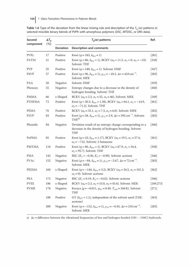
Table 1.6 Type of the deviation from the linear mixing rule and description of the Tg (w) patterns inselected miscible binary blends of PVPh with amorphous polymers (DSC, MTDSC, or DRS data).

Secondcomponent

ΔTg(°C)

Tg(w) patterns Ref.

Deviation Description and comments

PVPy 17 Positive Kwei (q= 183, kKw= 1) [281]

PATM 21 Positive Kwei (q= 86, kKw= 1), BCKV (α0= 11.5, α1= 0, α2=�33).Solvent: THF

[358]

PVP 25 Positive Kwei (q= 140, kKw= 1). Solvent: DMF [347]

P4VP 27 Positive Kwei (q= 96, kKw= 1), χ12=�18.2, Δv= 410 cm�1.Solvent: MEK

[283]

PAA 50 Negative Solvent: DMF [359]

Phenoxy 55 Negative Entropy changes due to a decrease in the density ofhydrogen bonding. Solvent: THF

[360]

PMMA 66 s-Shaped BCKV (α0= 2.3, α1= 55, α2= 46). Solvent: MEK [249]

PTHFMA 72 Positive Kwei (q= 30.3, kKw= 1.38), BCKV (α0= 64.1, α1=�14.9,α2=�71.2). Solvent: THF

[361]

PEMA 76 Positive BCKV (α0= 35.1, α1= 7.3, α2= 6.8). Solvent: MEK [282]

P2VP 83 Positive Kwei (q= 58, kKw= 1), χ12= 2.9, Δv= 395 cm�1. Solvent:THFa)

[283]

Phenolic 84 Negative Deviation result of an entropy change corresponding to adecrease in the density of hydrogen bonding. Solvent:THF

[360]

PnPMA 85 Positive Kwei (q= 10, kKw= 1.17), BCKV (α0= 19.5, α1= 57.4,α2=�7.6). Solvent: 2-butanone

[361]

PMTMA 118 Positive Kwei (q= 86, kKw= 1), BCKV (α0= 67.9, α1= 54.4,α2= 95.7). Solvent: THF

[358]

PMA 143 Negative BSC (K1=�0.36, K2=�0.90). Solvent: acetone [346]

PVAc 152 Negative Kwei (q=�84, kKw= 1), χ12=�2.67, Δv= 72 cm�1.Solvent: MEK

[283]

PEEMA 160 s-Shaped Kwei (q=�144, kKw= 3.2), BCKV (α0= 34.5, α1= 101.3,α2= 0). Solvent: acetone

[362]

PEA 172 Negative BSC (K1= 0.19, K2=�0.62). Solvent: acetone [346]

PVEE 186 s-Shaped BCKV (α0= 2.3, α1= 55.0, α2= 45.6). Solvent: MEK [249,273]

PVME 178 Negative Kovacs (g=�0.011, φ2c= 0.49, Tcrit= 344K). Solvent:THF

[271]

188 Positive GT (kGT= 1.1), independent of the solvent used (THF,acetone)

[363]

200 Negative Kwei (q=�152, kKw= 1), χ12=�0.45, Δv= 210 cm�1.Solvent: MEK

[283]

a) Δν= difference between the vibrational frequencies of free and hydrogen-bonded (OH ∙ ∙ ∙O��C) hydroxyls.


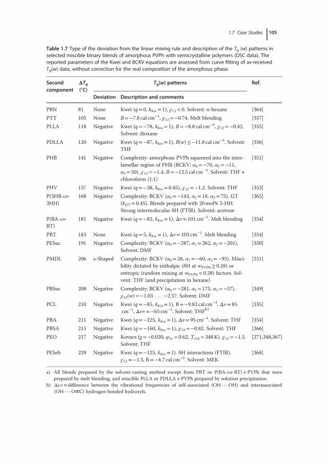
Table 1.7 Type of the deviation from the linear mixing rule and description of the Tg (w) patterns inselected miscible binary blends of amorphous PVPh with semicrystalline polymers (DSC data). Thereported parameters of the Kwei and BCKV equations are assessed from curve fitting of as-receivedTg(w) data, without correction for the real composition of the amorphous phase.

Secondcomponent

ΔTg(°C)

Tg(w) patterns Ref.

Deviation Description and comments

PBN 81 None Kwei (q= 0, kKw= 1), χ12< 0. Solvent: n-hexane [364]

PTT 105 None B=�7.8 cal cm�3, χ12=�0.74. Melt blending [357]

PLLA 118 Negative Kwei (q=�78, kKw= 1), B=�8.8 cal cm�3, χ12=�0.42.Solvent: dioxane

[355]

PDLLA 120 Negative Kwei (q=�87, kKw= 1), B(w)��11.8 cal cm�3. Solvent:THF

[356]

PHB 141 Negative Complexity: amorphous PVPh squeezed into the inter-lamellar region of PHB (BCKV: α0=�70, α1=�11,α2= 50). χ12=�1.4, B=�12.5 cal cm�3. Solvent: THF+chloroform (1:1)

[351]

PHV 157 Negative Kwei (q=�38, kKw= 0.45), χ12=�1.2. Solvent: THF [353]

P(3HB-co-3HH)

168 Negative Complexity: BCKV (α0=�143, α1= 18, α2= 75). GT(kGT= 0.45). Blends prepared with 20mol% 3-HH.Strong intermolecular δH (FTIR). Solvent: acetone

[365]

P(BA-co-BT)

181 Negative Kwei (q=�82, kKw= 1), Δv= 101 cm�1. Melt blending [354]

PBT 183 None Kwei (q= 5, kKw= 1), Δv= 103 cm�1. Melt blending [354]

PESuc 191 Negative Complexity: BCKV (α0=�287, α1= 262, α2=�201).Solvent: DMF

[350]

PMDL 206 s-Shaped Complexity: BCKV (α0= 28, α1=�60, α2=�95). Misci-bility dictated by enthalpic (δH at wPVPh� 0.28) orentropic (random mixing at wPVPh< 0.28) factors. Sol-vent: THF (and precipitation in hexane)

[251]

PBSuc 208 Negative Complexity: BCKV (α0=�281, α1= 175, α2=�57),χ12(w)=�1.03 . . . �2.57. Solvent: DMF

[349]

PCL 210 Negative Kwei (q=�85, kKw= 1), B=�9.82 cal cm�3, Δv= 85cm�1, Δv∗=�65 cm�1. Solvent: THFb)

[335]

PBA 211 Negative Kwei (q=�225, kKw= 1), Δv= 95 cm�1. Solvent: THF [354]

PBSA 215 Negative Kwei (q=�160, kKw= 1), χ12=�0.82. Solvent: THF [366]

PEO 217 Negative Kovacs (g=�0.020, φ2c= 0.62, Tcrit= 348K). χ12=�1.5.Solvent: THF

[271,348,367]

PESeb 229 Negative Kwei (q=�125, kKw= 1). δH interactions (FTIR).χ12=�1.3, B=�4.7 cal cm�3. Solvent: MEK

[368]

a) All blends prepared by the solvent-casting method except from PBT or P(BA-co-BT)+PVPh that wereprepared by melt blending, and miscible PLLA or PDLLA+PVPh prepared by solution precipitation.

b) Δν∗= difference between the vibrational frequencies of self-associated (OH ∙ ∙ ∙OH) and interassociated(OH ∙ ∙ ∙O��C) hydrogen-bonded hydroxyls.


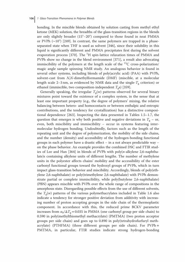
bonding. In the miscible blends obtained by solution casting from methyl ethylketone (MEK) solution, the breadths of the glass-transition regions in the blendsare only slightly broader (15°–20°) compared to those found in neat PMMAor PVPh (∼10°) [249]. In contrast, the same polymers are trapped in a phase-separated state when THF is used as solvent [346], since their solubility in thisliquid is significantly different and PMMA precipitates first during the solventevaporation process [370]. The 1H spin-lattice relaxation times of PMMA andPVPh show no change in the blend environment [371], a result also advocatingimmiscibility of the polymers at the length scale of the 13C cross-polarization/magic angle sample spinning NMR study. An analogous behavior is found inseveral other systems, including blends of poly(acrylic acid) (PAA) with PVPh,solvent-cast from N,N-dimethylformamide (DMF) (miscible, at a molecularlength scale 2–3 nm, as evidenced by NMR data and the single-Tg criterion) orethanol (immiscible, two composition-independent Tgs) [359].Generally speaking, the irregular Tg(w) patterns observed for several binary

mixtures point toward the existence of a complex system, in the sense that atleast one important property (e.g., the degree of polymers’ mixing, the relativebalancing between hetero- and homocontacts or between enthalpic and entropiccontributions, and the tendency for crystallization) has a distinctive composi-tional dependence [263]. Inspecting the data presented in Tables 1.5–1.7, thequestion that emerges is why both positive and negative deviations in Tg – or,even, both miscibility and immiscibility – occur in systems featuring inter-molecular hydrogen bonding. Undoubtedly, factors such as the length of therepeating unit and the degree of polymerization, the mobility of the side chains,and the number (density) and accessibility of the hydrogen-bonding functionalgroups in each polymer have a drastic effect – in a not always predictable way –on the phase behavior. An example provides the combined DSC and FTIR stud-ies of Lee and Han [364] in blends of PVPh with poly(n-alkylene 2,6-naphtha-late)s containing alkylene units of different lengths. The number of methyleneunits in the polyester affects chains’ mobility and the accessibility of the estercarbonyl functional groups toward the hydroxyl groups of PVPh, which in turnimpact glass-transition behavior and miscibility. Accordingly, blends of poly(eth-ylene 2,6-naphthalate) or poly(trimethylene 2,6-naphthalate) with PVPh demon-strate partial or complete immiscibility, while poly(butylene 2,6-naphthalate)(PBN) appears miscible with PVPh over the whole range of compositions in theamorphous state. Disregarding possible effects from the use of different solvents,the Tg(w) patterns of the various polymethacrylates included in Table 1.6 alsoindicate a tendency for stronger positive deviation from additivity with increas-ing number of proton accepting groups in the side chain of the thermoplasticcomponent. In accordance with this, the reduced prime BCKV parameterincreases from α0/ΔTg= 0.035 in PMMA (one carbonyl group per side chain) to0.590 in poly(methylthiomethyl methacrylate) (PMTMA) (two proton acceptorgroups per side chain) and goes up to 0.890 in poly(tetrahydrofurfuryl meth-acrylate) (PTHFMA) (three different groups per side chain). For PVPh+PMTMA, in particular, FTIR studies indicate strong hydrogen-bonding


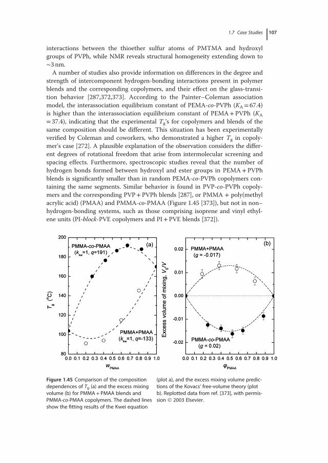
interactions between the thioether sulfur atoms of PMTMA and hydroxylgroups of PVPh, while NMR reveals structural homogeneity extending down to∼3 nm.A number of studies also provide information on differences in the degree and

strength of intercomponent hydrogen-bonding interactions present in polymerblends and the corresponding copolymers, and their effect on the glass-transi-tion behavior [287,372,373]. According to the Painter–Coleman associationmodel, the interassociation equilibrium constant of PEMA-co-PVPh (KA= 67.4)is higher than the interassociation equilibrium constant of PEMA+PVPh (KA

= 37.4), indicating that the experimental Tg’s for copolymers and blends of thesame composition should be different. This situation has been experimentallyverified by Coleman and coworkers, who demonstrated a higher Tg in copoly-mer’s case [272]. A plausible explanation of the observation considers the differ-ent degrees of rotational freedom that arise from intermolecular screening andspacing effects. Furthermore, spectroscopic studies reveal that the number ofhydrogen bonds formed between hydroxyl and ester groups in PEMA+PVPhblends is significantly smaller than in random PEMA-co-PVPh copolymers con-taining the same segments. Similar behavior is found in PVP-co-PVPh copoly-mers and the corresponding PVP+PVPh blends [287], or PMMA + poly(methylacrylic acid) (PMAA) and PMMA-co-PMAA (Figure 1.45 [373]), but not in non–hydrogen-bonding systems, such as those comprising isoprene and vinyl ethyl-ene units (PI-block-PVE copolymers and PI+PVE blends [372]).

Figure 1.45 Comparison of the compositiondependences of Tg (a) and the excess mixingvolume (b) for PMMA+ PMAA blends andPMMA-co-PMAA copolymers. The dashed linesshow the fitting results of the Kwei equation

(plot a), and the excess mixing volume predic-tions of the Kovacs’ free-volume theory (plotb). Replotted data from ref. [373], with permis-sion 2003 Elsevier.


1.7.2

Microstructure of the Amorphous Phase in Semicrystalline Blends

Blending of crystalline with amorphous polymers is a convenient way for thedevelopment of amorphous–crystalline interfaces and various morphologicalpatterns, which may result in an improvement of several physical properties(e.g., toughness, ductility, and impact strength). Although the miscibility windowand structural morphologies of related systems have been methodicallydescribed in time course, intense research activity is still engaged in studies ofaspects of the segregation between the crystalline/amorphous interface and ofthe possible relationships between intercomponent interactions and domain sizeof the separated phases. Detection of a single glass transformation range is typi-cal of the nonrigid (bulk-like) miscible amorphous phase, formed by the amor-phous fraction of the crystalline polymer and the amorphous component, withmiscibility achievement generally interpreted as a result of specific (hydrogenbonding [335]) or nonspecific interchain interactions, or by simply invoking thematched polarity of the blend components [374].The aliphatic polyester PCL provides an illustrative paradigm of technologi-

cally important semicrystalline polymers, offering a potential replacement forconventional polymers due to its biodegradability and low-temperature adhe-siveness. PCL is known for its ability to provide miscible blends with polymers,such as chlorinated polyethylenes [375], PVC [376], PC [377], SAN (with8–28 wt.% acrylonitrile) [378,379], poly(styrene-co-maleic anhydride) (PSMAn,with 14mol% maleic anhydride) [325], poly(styrene-co-vinylphenol) (with>13mol% of VPh in the copolymer) [380], poly(benzyl methacrylate) (PBzMA),and poly(phenyl methacrylate) (PPhMA) [374], PVME, phenolic, phenoxy, andPVPh [335,381–383] (Table 1.8). Several studies reveal interrelations among theextent of partial crystallization and the glass-transition temperature of the amor-phous phase. Rim and Runt [380], for example, observed that the greater theSAN concentration in PCL+ SAN blends, the higher the Tg and the lower thetendency for PCL crystallization. FTIR spectroscopy provides links between ther-mophysical properties (Tg and Tm) and the structural organization of phases incrystalline-amorphous blends exhibiting specific interactions. The stretchingvibrations of the carbonyl group of PCL and proton donating (e.g., hydroxyl)groups in several amorphous counterparts provide excellent probes of inter-molecular interactions. For instance, based on estimates of the Kwei parameter,q, the average strengths of the intermolecular interactions in blends of PCL withphenolic, PVPh, and phenoxy are weaker than the corresponding self-associationfor the homopolymers: q=�10 (phenolic)>�85 (PVPh)>�100 (phenoxy)(Kwei fits for kKw= 1) [335]. From a thermodynamic viewpoint, the strength ofthe specific interaction in a blend can also be described by its interaction energydensity parameter, B, which is obtained from the depression in the equilibriummelting point based on the Nishi–Wang equation. The negative values of B(�12.51, �9.82, and �7.55 cal cm�3 for blends with phenolic, PVPh, and phe-noxy, respectively) and the single glass-transition signals obtained are indicative


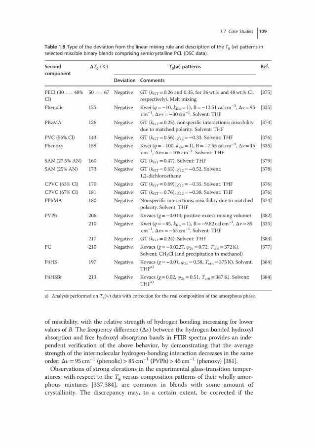
of miscibility, with the relative strength of hydrogen bonding increasing for lowervalues of B. The frequency difference (Δν) between the hydrogen-bonded hydroxylabsorption and free hydroxyl absorption bands in FTIR spectra provides an inde-pendent verification of the above behavior, by demonstrating that the averagestrength of the intermolecular hydrogen-bonding interaction decreases in the sameorder: Δν= 95 cm�1 (phenolic)> 85 cm�1 (PVPh)> 45 cm�1 (phenoxy) [381].Observations of strong elevations in the experimental glass-transition temper-

atures, with respect to the Tg versus composition patterns of their wholly amor-phous mixtures [337,384], are common in blends with some amount ofcrystallinity. The discrepancy may, to a certain extent, be corrected if the

Table 1.8 Type of the deviation from the linear mixing rule and description of the Tg (w) patterns inselected miscible binary blends comprising semicrystalline PCL (DSC data).

Secondcomponent

ΔTg (°C) Tg(w) patterns Ref.

Deviation Comments

PECl (30 . . . 48%Cl)

50 . . . 67 Negative GT (kGT= 0.26 and 0.35, for 36wt.% and 48wt.% Cl,respectively). Melt mixing

[375]

Phenolic 125 Negative Kwei (q=�10, kKw= 1), B=�12.51 cal cm�3, Δv= 95cm�1, Δv∗=�30 cm�1. Solvent: THF

[335]

PBzMA 126 Negative GT (kGT= 0.25), nonspecific interactions; miscibilitydue to matched polarity. Solvent: THF

[374]

PVC (56% Cl) 143 Negative GT (kGT= 0.56), χ12=�0.33. Solvent: THF [376]

Phenoxy 159 Negative Kwei (q=�100, kKw= 1), B=�7.55 cal cm�3, Δv= 45cm�1, Δv∗=�105 cm�1. Solvent: THF

[335]

SAN (27.5% AN) 160 Negative GT (kGT= 0.47). Solvent: THF [379]

SAN (25% AN) 173 Negative GT (kGT= 0.63), χ12=�0.52. Solvent:1,2-dichloroethane

[378]

CPVC (63% Cl) 170 Negative GT (kGT= 0.69), χ12=�0.35. Solvent: THF [376]

CPVC (67% Cl) 181 Negative GT (kGT= 0.76), χ12=�0.38. Solvent: THF [376]

PPhMA 180 Negative Nonspecific interactions; miscibility due to matchedpolarity. Solvent: THF

[374]

PVPh 206 Negative Kovacs (g=�0.014; positive excess mixing volume) [382]

210 Negative Kwei (q=�85, kKw= 1), B=�9.82 cal cm�3, Δv= 85cm�1, Δv∗=�65 cm�1. Solvent: THF

[335]

217 Negative GT (kGT= 0.24). Solvent: THF [383]

PC 210 Negative Kovacs (g=�0.0227, φ2c= 0.72, Tcrit= 372K).Solvent: CH3Cl (and precipitation in methanol)

[377]

P4HS 197 Negative Kovacs (g=�0.01, φ2c= 0.58, Tcrit= 375K). Solvent:THFa)

[384]

P4HSBr 213 Negative Kovacs (g= 0.02, φ2c= 0.51, Tcrit= 387K). Solvent:THFa)

[384]

a) Analysis performed on Tg(w) data with correction for the real composition of the amorphous phase.


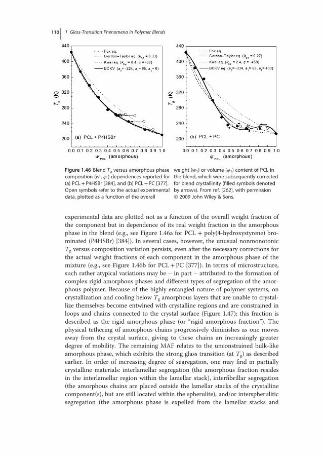
experimental data are plotted not as a function of the overall weight fraction ofthe component but in dependence of its real weight fraction in the amorphousphase in the blend (e.g., see Figure 1.46a for PCL + poly(4-hydroxystyrene) bro-minated (P4HSBr) [384]). In several cases, however, the unusual nonmonotonicTg versus composition variation persists, even after the necessary corrections forthe actual weight fractions of each component in the amorphous phase of themixture (e.g., see Figure 1.46b for PCL+PC [377]). In terms of microstructure,such rather atypical variations may be – in part – attributed to the formation ofcomplex rigid amorphous phases and different types of segregation of the amor-phous polymer. Because of the highly entangled nature of polymer systems, oncrystallization and cooling below Tg amorphous layers that are unable to crystal-lize themselves become entwined with crystalline regions and are constrained inloops and chains connected to the crystal surface (Figure 1.47); this fraction isdescribed as the rigid amorphous phase (or “rigid amorphous fraction”). Thephysical tethering of amorphous chains progressively diminishes as one movesaway from the crystal surface, giving to these chains an increasingly greaterdegree of mobility. The remaining MAF relates to the unconstrained bulk-likeamorphous phase, which exhibits the strong glass transition (at Tg) as describedearlier. In order of increasing degree of segregation, one may find in partiallycrystalline materials: interlamellar segregation (the amorphous fraction residesin the interlamellar region within the lamellar stack), interfibrillar segregation(the amorphous chains are placed outside the lamellar stacks of the crystallinecomponent(s), but are still located within the spherulite), and/or interspheruliticsegregation (the amorphous phase is expelled from the lamellar stacks and

Figure 1.46 Blend Tg versus amorphous phasecomposition (w´ , φ´) dependences reported for(a) PCL+ P4HSBr [384], and (b) PCL+ PC [377].Open symbols refer to the actual experimentaldata, plotted as a function of the overall

weight (w1) or volume (φ1) content of PCL inthe blend, which were subsequently correctedfor blend crystallinity (filled symbols denotedby arrows). From ref. [262], with permission 2009 John Wiley & Sons.


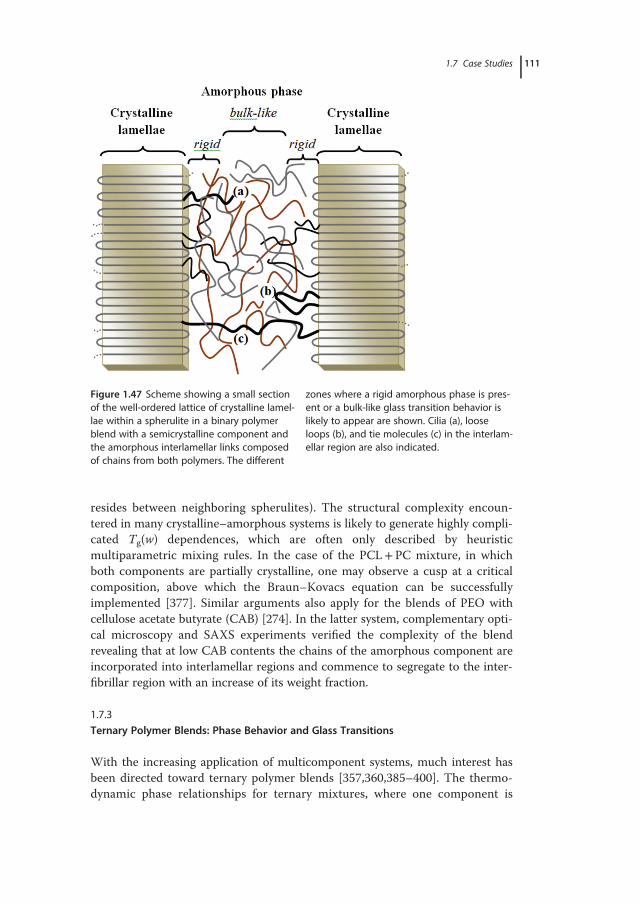
resides between neighboring spherulites). The structural complexity encoun-tered in many crystalline–amorphous systems is likely to generate highly compli-cated Tg(w) dependences, which are often only described by heuristicmultiparametric mixing rules. In the case of the PCL+PC mixture, in whichboth components are partially crystalline, one may observe a cusp at a criticalcomposition, above which the Braun–Kovacs equation can be successfullyimplemented [377]. Similar arguments also apply for the blends of PEO withcellulose acetate butyrate (CAB) [274]. In the latter system, complementary opti-cal microscopy and SAXS experiments verified the complexity of the blendrevealing that at low CAB contents the chains of the amorphous component areincorporated into interlamellar regions and commence to segregate to the inter-fibrillar region with an increase of its weight fraction.

1.7.3

Ternary Polymer Blends: Phase Behavior and Glass Transitions

With the increasing application of multicomponent systems, much interest hasbeen directed toward ternary polymer blends [357,360,385–400]. The thermo-dynamic phase relationships for ternary mixtures, where one component is

Figure 1.47 Scheme showing a small sectionof the well-ordered lattice of crystalline lamel-lae within a spherulite in a binary polymerblend with a semicrystalline component andthe amorphous interlamellar links composedof chains from both polymers. The different

zones where a rigid amorphous phase is pres-ent or a bulk-like glass transition behavior islikely to appear are shown. Cilia (a), looseloops (b), and tie molecules (c) in the interlam-ellar region are also indicated.


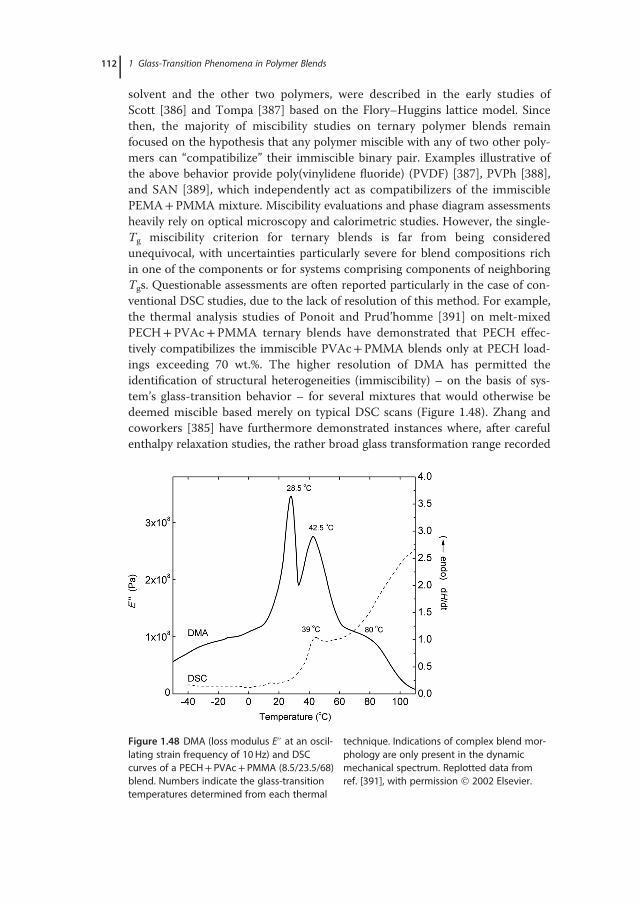
solvent and the other two polymers, were described in the early studies ofScott [386] and Tompa [387] based on the Flory–Huggins lattice model. Sincethen, the majority of miscibility studies on ternary polymer blends remainfocused on the hypothesis that any polymer miscible with any of two other poly-mers can “compatibilize” their immiscible binary pair. Examples illustrative ofthe above behavior provide poly(vinylidene fluoride) (PVDF) [387], PVPh [388],and SAN [389], which independently act as compatibilizers of the immisciblePEMA+PMMA mixture. Miscibility evaluations and phase diagram assessmentsheavily rely on optical microscopy and calorimetric studies. However, the single-Tg miscibility criterion for ternary blends is far from being consideredunequivocal, with uncertainties particularly severe for blend compositions richin one of the components or for systems comprising components of neighboringTgs. Questionable assessments are often reported particularly in the case of con-ventional DSC studies, due to the lack of resolution of this method. For example,the thermal analysis studies of Ponoit and Prud’homme [391] on melt-mixedPECH+PVAc+PMMA ternary blends have demonstrated that PECH effec-tively compatibilizes the immiscible PVAc+PMMA blends only at PECH load-ings exceeding 70 wt.%. The higher resolution of DMA has permitted theidentification of structural heterogeneities (immiscibility) – on the basis of sys-tem’s glass-transition behavior – for several mixtures that would otherwise bedeemed miscible based merely on typical DSC scans (Figure 1.48). Zhang andcoworkers [385] have furthermore demonstrated instances where, after carefulenthalpy relaxation studies, the rather broad glass transformation range recorded

Figure 1.48 DMA (loss modulus E´´ at an oscil-lating strain frequency of 10Hz) and DSCcurves of a PECH+ PVAc+ PMMA (8.5/23.5/68)blend. Numbers indicate the glass-transitiontemperatures determined from each thermal

technique. Indications of complex blend mor-phology are only present in the dynamicmechanical spectrum. Replotted data fromref. [391], with permission 2002 Elsevier.


for particular ternary blend compositions transforms to a multipart signal.Despite the apparent limitations of the glass-transition approach, related studiesremain at the frontline of miscibility evaluations of ternary blends. In such cases,however, it seems appropriate to consider the effect of the compatibilizer toinvolve a reduction of the size of the heterogeneous domains to a value compa-rable to the probe size of the particular measuring technique.When all three binary pairs are miscible, completely homogeneous ternary

blends or close immiscibility loop phase diagrams are possible. In general, in theabsence of strong specific interactions between the components, the ternaryphase behavior of polymer blend systems is primarily governed by differences inthe physical interaction among the components, which is expressed by the mag-nitude of the binary interaction parameters, χij (or equivalent solubility parame-ters, δi). If just one of the binary interaction parameters is significantly largerthan a critical value [385], a large portion of the ternary phase diagram is pre-dicted to be heterogeneous. In addition, a strong driving force toward phase sep-aration exists if there are significant differences in the solubility or interactionparameter values (i.e., χij� χik 6� 0), which produces the so-called “Δχ effect”. Interms of the Painter–Coleman association model, the effect of strong specificinteractions (hydrogen bonds) on the phase behavior is considered to be con-trolled by the magnitudes of the equilibrium constants describing self- and inter-association, and the difference between the effective interassociation equilibriumconstants of the binary systems (ΔK). The latter is usually called the “ΔK effect”and reflects the difference in the “chemical” interaction between the self-associ-ating polymer and the other polymers in the mixture; a strong ΔK effect isresponsible for phase separation. Bearing in mind the above restrictions, onlyvery few ternary polymer blends are expected to be homogeneous over theirentire range of compositions. These “totally” miscible, ternary blends – includingPVDF+PVAc+PMMA [390], PECH+PMMA+PEO [392], PHB+PEO+PECH [393], poly(ether diphenyl ether ketone)+ poly(ether ether ketone)+PEI [394], PEI+PET+PBT [395], and PCL+PPhMA+PBzMA [396] – all pos-sess low Δχ effects and no hydrogen-bonding interactions between their seg-ments (i.e., the ΔK effect can be neglected).Addition of a polymeric component capable of forming strong hydrogen-

bonding interactions (i.e., a proton donor) may potentially act as a mutual com-mon link for the other polymers (containing proton-accepting functionalgroups), leading to a “bridging effect” and the formation of a more homogeneousternary mixture. For this to happen, however, it is essential that the inter-association equilibrium constants of the two miscible hydrogen-bonding binariesare comparable. Thermal analyses, for example, have provided compelling evi-dence of phase homogeneity for all blend compositions in ternary blends ofPVPh with PVAc and PMA [385], or with pairs of homologous aryl polyesters(PET, PTT, or PBT) [357]. In all these ternary systems, ultimate miscibility isaccredited to negligible differences in the level of the physical interactionsamong their components (no Δχ effect), and the sensitive balancing of thehydrogen-bonding interactions in the ternary blends between PVPh and either


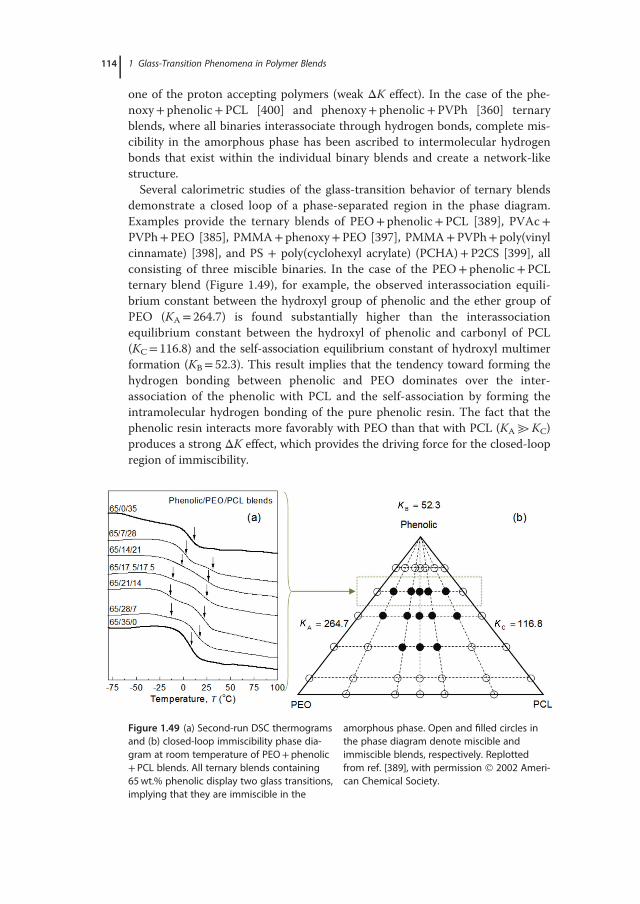
one of the proton accepting polymers (weak ΔK effect). In the case of the phe-noxy+ phenolic+PCL [400] and phenoxy+ phenolic+PVPh [360] ternaryblends, where all binaries interassociate through hydrogen bonds, complete mis-cibility in the amorphous phase has been ascribed to intermolecular hydrogenbonds that exist within the individual binary blends and create a network-likestructure.Several calorimetric studies of the glass-transition behavior of ternary blends

demonstrate a closed loop of a phase-separated region in the phase diagram.Examples provide the ternary blends of PEO+ phenolic+PCL [389], PVAc+PVPh+PEO [385], PMMA+ phenoxy+PEO [397], PMMA+PVPh+ poly(vinylcinnamate) [398], and PS + poly(cyclohexyl acrylate) (PCHA)+P2CS [399], allconsisting of three miscible binaries. In the case of the PEO+ phenolic+PCLternary blend (Figure 1.49), for example, the observed interassociation equili-brium constant between the hydroxyl group of phenolic and the ether group ofPEO (KA= 264.7) is found substantially higher than the interassociationequilibrium constant between the hydroxyl of phenolic and carbonyl of PCL(KC= 116.8) and the self-association equilibrium constant of hydroxyl multimerformation (KB= 52.3). This result implies that the tendency toward forming thehydrogen bonding between phenolic and PEO dominates over the inter-association of the phenolic with PCL and the self-association by forming theintramolecular hydrogen bonding of the pure phenolic resin. The fact that thephenolic resin interacts more favorably with PEO than that with PCL (KA@KC)produces a strong ΔK effect, which provides the driving force for the closed-loopregion of immiscibility.

Figure 1.49 (a) Second-run DSC thermogramsand (b) closed-loop immiscibility phase dia-gram at room temperature of PEO+phenolic+ PCL blends. All ternary blends containing65wt.% phenolic display two glass transitions,implying that they are immiscible in the

amorphous phase. Open and filled circles inthe phase diagram denote miscible andimmiscible blends, respectively. Replottedfrom ref. [389], with permission 2002 Ameri-can Chemical Society.


1.8Concluding Remarks

The reversible transformation of amorphous materials from a devitrified orviscoelastic (rubber-like) state into the fairly brittle state of solid glass consti-tutes one of the most puzzling phenomena in materials science. The distinctkinetic and thermodynamic aspects of the glass transition and the diverseexperimental responses recorded hitherto for polymers under differentmolecular environments and geometric constrictions hamper a unified theo-retical interpretation of the event. Regardless of the practically imperceptiblestructural changes during the transition, numerous experimental techniquesemploying thermal, mechanical, electrical, or electromagnetic excitation ofspecific molecular motions have provided compelling evidence of the drasticchanges in segmental mobility and molecular bonding that occur in the glasstransformation range. Thermal analysis techniques are particularly effectivein determining characteristics of the cooperative molecular motions activat-ing in the glass transformation range, with numerous studies indicating thatthe location and width of the respective transitions are regulated by inherentproperties of the material (chemical structure, chain architecture, free vol-ume, etc.), in addition to a number of externally controlled factors (pressure,additives, level of confinement, etc.).The variability of motional probes and the ensuing differences in the prob-

ing length scale of the various measuring techniques, the broadly differentoscillation frequencies used in popular isochronal dynamic experiments,along with the different (often inappropriate) procedures adopted for condi-tioning the testing materials, may become sources of misperception – ratherthan power tools – in the hands of the novice experimentalist. Notwithstand-ing the above complications, the glass-transition phenomenon and its defin-ing marker, the glass-transition temperature, have for long been explored andused to evaluate the success of polymers’ mixing. The resulting materialsexhibit properties intermediate or even superior to those of their pure com-ponents, offering a means to improve the poor performances of existing poly-mers without sacrificing any excellent characteristic. The paradigmsillustrated in this chapter make evident that the number of transitions andthe compositional dependence of the respective glass-transition temperaturesoffer indicators of miscibility, partial miscibility (compatibility), orimmiscibility between blend components. The conventional – althoughsomewhat misused – experimental criterion for determining miscibility inpolymer blends is based on the measurement of a single glass-transition sig-nal for all blend compositions, usually located in between the glass-transitiontemperatures of the components and consistent with the composition of theblend. For miscible binary polymer systems, in particular, the various theoret-ical or phenomenological approaches critically examined in this chapter haveformulated different analytical Tg(w) functions, endorsing as a minimumqualitative correlations of their parameters with miscibility-controlling

1.8 Concluding Remarks 115

factors, such as the type and strength of intercomponent interactions, the rel-ative balancing between inter- and intramolecular interactions, conforma-tional entropy changes, or the magnitude and partition of the excess mixingvolume in the system. In the case of the partially miscible or compatibilizedpolymer blends, the glass transitions of both components are recorded. Con-vergence of the glass-transition temperatures of the two phases is typicallyobserved, along with a change in the width and the strength of the signals.Interestingly, an analogous behavior often emerges in dynamically heteroge-neous blends of weakly interacting components, with the level of homogene-ity approaching the segmental length scale. Moreover, dynamic studies ofpartially mixed systems reveal shifts in the glass-transition temperatures andchanges in the width of the transition signals, which provide a measure of theextent of molecular mixing. In contrast, complete segregation of phases(immiscibility) is evidenced by separate glass transitions for all blend compo-sitions, with nearly composition-independent transition temperatures.The reproducibility and appropriate resolution of the complex glass transition

data obtained in several polymer-based composites is prerequisite for achievingunambiguous experimental determinations of structural homogeneity or of thestate of dispersion in multiphase systems. The cases discussed in this chapteremphasize the need for testing materials that have attained equilibrium condi-tions prior to the experiment; that is, the thermal, mechanical or electrical his-tory (memory effects) has to be erased, following standard pretreatments.Moreover, optimal mixing conditions, which include appropriately selected typeand amount of solvent(s), temperature of mixing, and method of preparation(i.e., solvent evaporation, coprecipitation or hot-melt extrusion), are essential.Experimental attempts to establish the miscibility window of any pair of poly-mers via their glass-transition behavior have to consider also the nature, sensitiv-ity, and resolution of the probing technique, the latter being directly related tothe limiting domain size with distinguishable thermal response. Along theselines, blends displaying a single glass transition may be deemed miscible only ona scale at or above the total number of segments cooperatively relaxing at theglass transition (i.e., determined level of homogeneity no less than the probelength scale of the particular technique). The issues presented in several sectionsof this chapter reveal that proper identification of glass transitions entails rigor-ous separation of the pertinent signals from neighboring transitions (e.g., meltingpeaks, liquid–liquid transitions), relaxational phenomena (secondary relaxations,interfacial polarizations, enthalpy, or volume relaxation, etc.), or other signals(e.g., noise, background), and subsequent analysis following appropriate models.Unfortunately, despite the advent of modulated temperature techniques in manyfields of thermal analysis along with the introduction of novel commercial exper-imental systems with remarkable accuracy and signal-resolving power, properconsideration of the above issues is often lacking in routine experiments. Thissituation may cast doubts in several evaluations and precludes straightforwardcomparisons among seemingly complementary studies of glass formation andpolymer dynamics in complex systems.


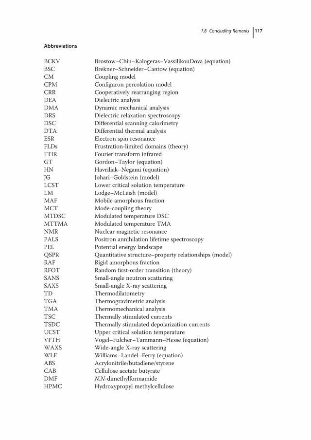
Abbreviations

BCKV Brostow–Chiu–Kalogeras–VassilikouDova (equation)BSC Brekner–Schneider–Cantow (equation)CM Coupling modelCPM Configuron percolation modelCRR Cooperatively rearranging regionDEA Dielectric analysisDMA Dynamic mechanical analysisDRS Dielectric relaxation spectroscopyDSC Differential scanning calorimetryDTA Differential thermal analysisESR Electron spin resonanceFLDs Frustration-limited domains (theory)FTIR Fourier transform infraredGT Gordon–Taylor (equation)HN Havriliak–Negami (equation)JG Johari–Goldstein (model)LCST Lower critical solution temperatureLM Lodge–McLeish (model)MAF Mobile amorphous fractionMCT Mode-coupling theoryMTDSC Modulated temperature DSCMTTMA Modulated temperature TMANMR Nuclear magnetic resonancePALS Positron annihilation lifetime spectroscopyPEL Potential energy landscapeQSPR Quantitative structure–property relationships (model)RAF Rigid amorphous fractionRFOT Random first-order transition (theory)SANS Small-angle neutron scatteringSAXS Small-angle X-ray scatteringTD ThermodilatometryTGA Thermogravimetric analysisTMA Thermomechanical analysisTSC Thermally stimulated currentsTSDC Thermally stimulated depolarization currentsUCST Upper critical solution temperatureVFTH Vogel–Fulcher–Tammann–Hesse (equation)WAXS Wide-angle X-ray scatteringWLF Williams–Landel–Ferry (equation)ABS Acrylonitrile/butadiene/styreneCAB Cellulose acetate butyrateDMF N,N-dimethylformamideHPMC Hydroxypropyl methylcellulose


HPMCAS Hydroxypropyl methylcellulose acetate succinateMnSPS Manganese sulfonated PS (10.1mol% of MnS in PS)PαMS Poly(α-methyl styrene)P(3HB-co-3HH) Poly(3-hydroxybutyrate-co-3-hydroxyhexanoate)P(BA-co-BT) Poly(butylene adipate-co-butylene terephthalate))P(VP-co-VA) Poly(vinyl pyrrolidone-co-vinyl acetate)P2CS Poly(2-chloro styrene)P2VP Poly(2-vinyl pyridine)P4HS Poly(4-hydroxystyrene)P4HSBr Poly(4-hydroxystyrene) brominatedP4tBS Poly(4-tert-butylstyrene)P4VP Poly(4-vinyl pyridine)PA-6 Polyamide-6PATM Poly(N-acryloylthiomorpholine)PB PolybutadienePBA Poly(butylene adipate)PBN Poly(butylene 2,6-naphthalate)PBSA Poly(butylene succinate-co-butylene adipate)PBSuc Poly(butylene succinate)PBT Poly(butylene terephthalate)PBzMA Poly(benzyl methacrylate)PC PolycarbonatePCHA Poly(cyclohexyl acrylate)PCHMA Poly(cyclohexyl methacrylate)PCL Poly(ε-caprolactone)PDLLA Poly(D,L-lactide)PE PolyethylenePEA Poly(ethylene adipate)PECH Poly(epichlorohydrine)PECl Chlorinated polyethylenePEEMA Poly(2-ethoxyethyl methacrylate)PEKK Poly(ether ketone ketone)PEMA Poly(ethyl methacrylate)PEO Polyethylene oxidePESeb Poly(ethylene sebacate)PESuc Poly(ethylene succinate)PET Poly(ethylene terephthalate)PHB Poly(β-hydroxybutyrate)Phenolic Phenolic resinPhenoxy Poly(hydroxylether of bisphenol A)PHV Poly(hydroxyvalerate)PI PolyisoprenePLLA Poly(L-lactide)PMA Poly(methyl acrylate)PMDL Poly(N-methyldodecano-12-lactam)


PMAA Poly(methyl acrylic acid)PMMA Poly(methyl methacrylate)PMTMA Poly(methylthiomethyl methacrylate)PNB PolynorbornenePnPMA Poly(n-propyl methacrylate)PoCS Poly(o-chlorostyrene)PP PolypropylenePPE Poly(2,6-dimethylphenylene ether)PPhMA Poly(phenyl methacrylate)PPO Poly(2,6-dimethyl-1,4-phenylene oxide)PS PolystyrenePS4VP Poly(styrene-co-4-vinylpyridine)PSAA Poly(styrene-co-acrylic acid)PSAD poly(styrene-co-N,N-dimethylacrylamide)PSCA Poly(styrene-co-cinnamic acid)PSHS Poly(styrene-co-hydroxystyrene)PSMA Poly(styrene-co-methacrylic acid)PSMAn Poly(styrene-co-maleic anhydride)PTHFMA Poly(tetrahydrofurfuryl methacrylate)PTT Poly(trimethylene terephthalate)PVAc Poly(vinyl acetate)PVC Poly(vinyl chloride)PVDF Poly(vinylidene fluoride)PVE Poly(vinylethylene)PVEE Poly(vinyl ethyl ether)PVK Poly(N-vinyl carbazole)PVME Poly(vinyl methyl ether)PVP Poly(vinyl pyrrolidone)PVPh Poly(vinyl phenol)PVPhKH Poly(vinyl phenyl ketone hydrogenated)PVPy Poly(vinyl pyridine)SAN Poly(styrene-co-acrylonitrile)THF TetrahydrofuranTMPC Tetramethyl polycarbonateTPI Thermoplastic polyimide

Symbols

< . . . > Average valueA, B Material or model-specific constantsa0, a1, a2 Parameters of the BCKV equationB Interaction energy densityBi Fraction of flexible bonds of the ith polymerAT Amplitude of temperature modulationC, C1, C2 Model-specific constants


ci Model-specific parameters (i= 1, 2, . . . )Capp Apparent heat capacityCp Heat capacityD Thicknessd Dimension of spaceE∗ Complex modulus (E∗=E´ + iE´´)E EnergyF Free energy; acting forcef Free-volume fraction; scanning frequencyfg Free-volume fraction at Tg

fmax Peak frequency of the dynamic glass transition(α-relaxation)

E, Eact Energy; activation energyG Gibbs free energyG∗ Shear complex modulus (G∗=G´ + iG´´)g Interaction term (Kovacs’ model)H EnthalpyI CurrentK, K∗, k1, k2, k3 Material specific constantsKA, KC Interassociation equilibrium constantsKB Self-association equilibrium constantK1, K2 Parameters of the BSC equationk, kCK, kDM, kGT, kJH, kkw Parameters of various Tg(w) functionskb Amount of backbone bonds per repeat unitkβ Boltzmann constantL, l Lengthlk Kuhn lengthlb Length of the average backbone bondM∗ Complex modulusM0 Monomer (or repeat-unit) molar massMc Molar mass of chains between cross-linksMn Molar mass (number average)m Mass; fragility parameter (steepness index)mT Thermodynamic fragility (parameter)NA Avogadro’s numberNi Number of segments of the ith polymern Exponent (various models)P PressurePav Average probabilitypc Critical configurons concentrationQ Partition function; heatq Rate of temperature change; parameter (Kwei

equation)R Gas constantS Entropy


Sc Configurational entropysc∗ Critical configurational entropy

t TimeT Absolute temperatureTc Crystallization temperatureTcc Cold crystallization temperatureTMCT Critical temperature (MCT, RFOT)Tcrit Critical temperature (Kovacs’ model)Tf Fictive temperatureTg Glass-transition temperatureTK Kauzmann temperatureTLL Liquid–liquid transition temperatureTm Melting temperatureTr Reference temperatureTs Sample temperatureTV Vogel temperatureT0, T2 Sc-vanishing temperaturesTb, T1e, T2e, Te Different marks of glass-transition temperature in a

DSC curveT1ρ(H) Proton spin-lattice relaxation time in the rotational

frametan δ Loss tangent (E´´/E´, G´´/G´, ε´´/ε´)V VolumeVα Cooperativity volumeVf Free volumeVf

∗ Free volume at T<Tg

V0 Hardcore (or incompressible) molecular volumew Mass (or weight) fractionx Mole fractionz Size of CRR (Adam–Gibbs model)z∗ Critical size of CRR

Greek Symbols

α Coefficient of volumetric thermal expansionα Primary relaxation, dynamic glass transitionαc Degree of cureαf Coefficient of free-volume thermal expansionαL Coefficient of linear thermal expansionαT Temperature shift factor; thermal expansion coefficientβ, γ, δ Secondary relaxationsβKWW KWW function exponentγ Exponent (MCT)γi Number of flexible bonds per repeating unitΔCp Heat capacity change at the transition


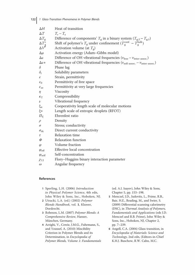
ΔH Heat of transitionΔT Tr�Ts

ΔTg Difference of components’ Tg in a binary system (Tg,2�Tg,1)ΔT∗

g Shift of polymer’s Tg under confinement �T conf :g � Tbulk

g �ΔV# Activation volume (at Tg)Δμ Activation energy (Adam–Gibbs model)Δν Difference of OH vibrational frequencies (vfree� vinter-assoc.)Δν∗ Difference of OH vibrational frequencies (vself-assoc.� vinter-assoc.)δ Phase lagδi Solubility parametersε Strain, permittivityε0 Permittivity of free spaceε1 Permittivity at very large frequenciesη ViscosityκT Compressibilityν Vibrational frequencyξα Cooperativity length scale of molecular motionsξ∗ Length scale of entropic droplets (RFOT)ΠE Ehrenfest ratioρ Densityσ Stress; conductivityσdc Direct current conductivityτ Relaxation timeΦ Relaxation functionφ Volume fractionφeff Effective local concentrationφself Self-concentrationχ12 Flory–Huggins binary interaction parameterω Angular frequency

References

1 Sperling, L.H. (2006) Introductionto Physical Polymer Science, 4th edn,John Wiley & Sons, Inc., Hoboken, NJ.

2 Utracki, L.A. (ed.) (2002) PolymerBlends Handbook, vol. 1, Kluwer,Dordrecht.

3 Robeson, L.M. (2007) Polymer Blends: AComprehensive Review, Hanser,München, Germany.

4 Arrighi, V., Cowie, J.M.G., Fuhrmann, S.,and Youssef, A. (2010) MiscibilityCriterion in Polymer Blends and itsDetermination, in Encyclopedia ofPolymer Blends, Volume 1: Fundamentals

(ed. A.I. Isayev), John Wiley & Sons,Chapter 5, pp. 153–198.

5 Menczel, J.D., Judovits, L., Prime, R.B.,Bair, H.E., Reading, M., and Swier, S.(2009) Differential scanning calorimetry(DSC), in Thermal Analysis of Polymers,Fundamentals and Applications (eds J.D.Menczel and R.B. Prime), John Wiley &Sons, Inc., Hoboken, NJ, Chapter 2,pp. 7–239.

6 Angell, C.A. (2004) Glass transition, inEncyclopedia of Materials: Science andTechnology, 2nd edn, (Editors-in-ChiefK.H.J. Buschow, R.W. Cahn, M.C.


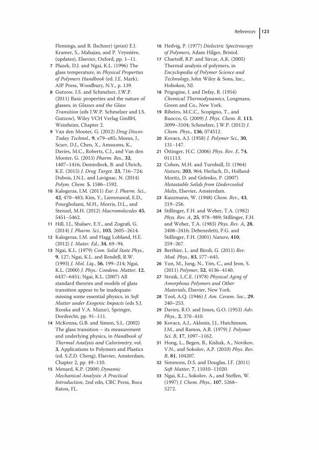
Flemings, and B. Ilschner) (print) E.J.Kramer, S., Mahajan, and P. Veyssière,(updates), Elsevier, Oxford, pp. 1–11.

7 Plazek, D.J. and Ngai, K.L. (1996) Theglass temperature, in Physical Propertiesof Polymers Handbook (ed. J.E. Mark),AIP Press, Woodbury, N.Y., p. 139.

8 Gutzow, I.S. and Schmelzer, J.W.P.(2011) Basic properties and the nature ofglasses, in Glasses and the GlassTransition (eds J.W.P. Schmelzer and I.S.Gutzow), Wiley VCH Verlag GmBH,Weinheim, Chapter 2.

9 Van den Mooter, G. (2012) Drug Discov.Today Technol., 9, e79–e85; Meeus, J.,Scurr, D.J., Chen, X., Amssoms, K.,Davies, M.C., Roberts, C.J., and Van denMooter, G. (2015) Pharm. Res., 32,1407–1416; Demirdirek, B. and Uhrich,K.E. (2015) J. Drug Target. 23, 716–724;Dubois, J.N.L. and Lavignac, N. (2014)Polym. Chem. 5, 1586–1592.

10 Kalogeras, I.M. (2011) Eur. J. Pharm. Sci.,42, 470–483; Kim, Y., Liemmawal, E.D.,Pourgholami, M.H., Morris, D.L., andStenzel, M.H. (2012) Macromolecules 45,5451–5462.

11 Hill, J.J., Shalaev, E.Y., and Zografi, G.(2014) J. Pharm. Sci., 103, 2605–2614.

12 Kalogeras, I.M. and Hagg Lobland, H.E.(2012) J. Mater. Ed., 34, 69–94.

13 Ngai, K.L. (1979) Com. Solid State Phys.,9, 127; Ngai, K.L. and Rendell, R.W.(1993) J. Mol. Liq., 56, 199–214; Ngai,K.L. (2000) J. Phys.: Condens. Matter, 12,6437–6451; Ngai, K.L. (2007) Allstandard theories and models of glasstransition appear to be inadequate:missing some essential physics, in SoftMatter under Exogenic Impacts (eds S.J.Rzoska and V.A. Mazur), Springer,Dordrecht, pp. 91–111.

14 McKenna, G.B. and Simon, S.L. (2002)The glass transition – its measurementand underlying physics, in Handbook ofThermal Analysis and Calorimetry, vol.3, Applications to Polymers and Plastics(ed. S.Z.D. Cheng), Elsevier, Amsterdam,Chapter 2, pp. 49–110.

15 Menard, K.P. (2008) DynamicMechanical Analysis: A PracticalIntroduction, 2nd edn, CRC Press, BocaRaton, FL.

16 Hedvig, P. (1977) Dielectric Spectroscopyof Polymers, Adam Hilger, Bristol.

17 Chartoff, R.P. and Sircar, A.K. (2005)Thermal analysis of polymers, inEncyclopedia of Polymer Science andTechnology, John Wiley & Sons, Inc.,Hoboken, NJ.

18 Prigogine, I. and Defay, R. (1954)Chemical Thermodynamics, Longmans,Green and Co., New York.

19 Ribeiro, M.C.C., Scopigno, T., andRuocco, G. (2009) J. Phys. Chem. B, 113,3099–3104; Schmelzer, J.W.P. (2012) J.Chem. Phys., 136, 074512.

20 Kovacs, A.J. (1958) J. Polymer Sci., 30,131–147.

21 Öttinger, H.C. (2006) Phys. Rev. E, 74,011113.

22 Cohen, M.H. and Turnbull, D. (1964)Nature, 203, 964; Herlach, D., Holland-Moritz, D. and Gelenko, P. (2007)Metastable Solids from UndercooledMelts, Elsevier, Amsterdam.

23 Kauzmann, W. (1948) Chem. Rev., 43,219–256.

24 Stillinger, F.H. and Weber, T.A. (1982)Phys. Rev. A, 25, 978–989; Stillinger, F.H.and Weber, T.A. (1983) Phys. Rev. A, 28,2408–2416; Debenedetti, P.G. andStillinger, F.H. (2001) Nature, 410,259–267.

25 Berthier, L. and Biroli, G. (2011) Rev.Mod. Phys., 83, 577–645.

26 Yun, M., Jung, N., Yim, C., and Jeon, S.(2011) Polymer, 52, 4136–4140.

27 Struik, L.C.E. (1978) Physical Aging ofAmorphous Polymers and OtherMaterials, Elsevier, New York.

28 Tool, A.Q. (1946) J. Am. Ceram. Soc., 29,240–253.

29 Davies, R.O. and Jones, G.O. (1953) Adv.Phys., 2, 370–410.

30 Kovacs, A.J., Aklonis, J.J., Hutchinson,J.M., and Ramos, A.R. (1979) J. PolymerSci. B, 17, 1097–1162.

31 Hong, L., Begen, B., Kisliuk, A., Novikov,V.N., and Sokolov, A.P. (2010) Phys. Rev.B, 81, 104207.

32 Simmons, D.S. and Douglas, J.F. (2011)Soft Matter, 7, 11010–11020.

33 Ngai, K.L., Sokolov, A., and Steffen, W.(1997) J. Chem. Phys., 107, 5268–5272.

References 123

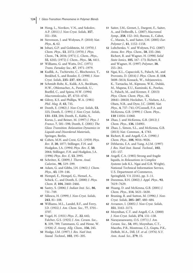
34 Hong, L., Novikov, V.N., and Sokolov,A.P. (2011) J. Non-Cryst. Solids, 357,351–356.

35 Stevenson, J. and Wolynes, P. (2010) Nat.Phys., 6, 62.

36 Johari, G.P. and Goldstein, M. (1970) J.Chem. Phys., 53, 2372; (1970) J. Phys.Chem., 74, 2034; (1971) J., Chem., Phys.,55, 4245; (1972) J. Chem., Phys., 56, 4411.

37 Williams, G. and Watts, D.C. (1971)Trans. Faraday Soc., 67, 1971–1979.

38 Kudlik, A., Tschirwitz, C., Blochowicz, T.,Benkhof, S., and Rossler, E. (1998) J. Non-Cryst. Solids, 235–237, 406–411.

39 Schmidt-Rohr, K., Kulik, A.S., Beckham,H.W., Ohlemacher, A., Pawelzik, U.,Boeffel, C., and Spiess, H.W. (1994)Macromolecules, 27, 4733–4745.

40 Gilroy, K.S. and Phillips, W.A. (1981)Phil. Mag. B, 43, 735.

41 Donth, E. (1982) J. Non-Cryst. Solids, 53,325; Donth, E. (1991) J. Non-Cryst. Solids,131–133, 204; Donth, E., Kahle, S.,Korus, J., and Beiner, M. (1997) J. Phys. IFrance, 7, 581–598; Donth, E. (2001) TheGlass Transition. Relaxation Dynamics inLiquids and Disordered Materials,Springer, Berlin.

42 Cohen, M.H. and Crest, G.S. (1959) Phys.Rev. B, 20, 1077; Stillinger, F.H. andHodgdon, J.A. (1994) Phys. Rev. E, 50,2064; Stillinger, F.H. and Hodgdon, J.A.(1996) Phys. Rev. E, 53, 2995.

43 Schröter, K. (2009) J. Therm. Anal.Calorim., 98, 519–599.

44 Adam, G. and Gibbs, J.H. (1965) J. Chem.Phys., 43, 139–146.

45 Hempel, E., Hempel, G., Hensel, A.,Schick, C., and Donth, E. (2000) J. Phys.Chem. B, 104, 2460–2466.

46 Sastry, S. (2006) J. Indian Inst. Sci., 86,731–749.

47 Sillescu, H. (1999) J. Non-Cryst. Solids,243, 81–108.

48 Williams, M.L., Landel, R.F., and Ferry,J.D. (1955) J. Am. Chem. Soc., 77, 3701–3707.

49 Vogel, H. (1921) Phys. Z., 22, 645;Fulcher, G.S. (1925) J. Am. Ceram. Soc.,8, 339, 789; Tammann, G. and Hesse, W.(1926) Z. Anorg. Allg. Chem., 156, 245.

50 Hodge, I.M. (1997) J. Res. Natl Inst.Stand. Technol., 102, 195–205.

51 Saiter, J.M., Grenet, J., Dargent, E., Saiter,A., and Delbreilh, L. (2007) Macromol.Symp., 258, 152–161; Bureau, E., Cabot,C., Marais, S., and Saiter, J.M. (2005) Eur.Polymer J., 41, 1152–1158.

52 Lubchenko, V. and Wolynes, P.G. (2007)Annu. Rev. Phys. Chem., 58, 235–266;Richert, R. and Wagner, H. (1998) SolidState Ionics, 105, 167–173; Richert, R.and Wagner, H. (1997) Polymer, 38,255–261.

53 Ngai, K.L., Capaccioli, S., Paluch, M., andProvosto, D. (2014) J. Phys. Chem. B, 118,5608–5614; Kossack, W., Adrjanowicz,K., Tarnacka, M., Kipnusu, W.K., Dulski,M., Mapesa, E.U., Kaminski, K., Pawlus,S., Paluch, M., and Kremer, F. (2013)Phys. Chem. Chem. Phys., 15,20641–20650; Hecksher, T., Nielsen, A.I.,Olsen, N.B., and Dyre, J.C. (2008) Nat.Phys., 4, 737–741; O’Connell, P.A. andMcKenna, G.B. (1999) J. Chem. Phys.,110 11054–11060.

54 Zhao, J. and McKenna, G.B. (2012) J.Chem. Phys., 136, 154901.

55 Zhao, J., Simon, S.L., and McKenna, G.B.(2013) Nat. Commun., 4, 1783.

56 Richert, R. and Angell, C.A. (1998) J.Chem. Phys., 108, 9016–9026.

57 DiMarzio, E.A. and Yang, A.J.M. (1997)J. Res. Natl Inst. Stand. Technol., 102,135–157.

58 Angell, C.A. (1985) Strong and fragileliquids, in Relaxations in ComplexSystems (eds K.L. Ngai and G.B. Wright),National Technical Information Service,U.S. Department of Commerce,Springfield, VA 22161, pp. 3–11.

59 Doremus, R.H. (2002) J. Appl. Phys., 92,7619–7629.

60 Huang, D. and McKenna, G.B. (2001) J.Chem. Phys., 114, 5621–5630.

61 Bruning, R. and Sutton, M. (1996) J. Non-Cryst. Solids, 205–207, 480–484.

62 Avramov, I. (2005) J. Non-Cryst. Solids,351, 3163–3173.

63 Moynihan, C.T. and Angell, C.A. (2000)J. Non-Cryst. Solids, 274, 131–138.

64 Narayanaswamy, O.S. (1971) J. Am.Ceram. Soc., 54, 491; Moynihan, C.T.,Macebo, P.B., Montrose, C.J., Gupta, P.K.,DeBolt, M.A., Dill, J.F. et al. (1976) N.Y.Ann. Acad. Sci., 279, 15.


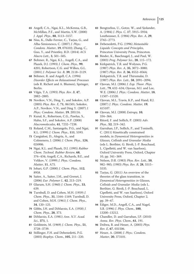
65 Angell, C.A., Ngai, K.L., McKenna, G.B.,McMillan, P.F., and Martin, S.W. (2000)J. Appl. Phys., 88, 3113–3157.

66 Niss, K., Dalle-Ferrier, C., Tarjus, G., andAlba-Simionesco, C. (2007) J. Phys.:Condens. Matter, 19, 076102; Zhang, C.,Guo, Y., and Priestley, R.D. (2014) ACSMacro Lett., 3, 501–505.

67 Bohmer, R., Ngai, K.L., Angell, C.A., andPlazek, D.J. (1993) J. Chem. Phys., 99,4201; Robertson, C.G. and Wilkes, G.L.(2001) J. Polymer Sci. B, 39, 2118–2129.

68 Böhmer, R. and Angell, C.A. (1994)Disorder Effects on Relaxational Processes(eds R. Richert and A. Blumen), Springer,Berlin.

69 Vilgis, T.A. (1993) Phys. Rev. B, 47,2882–2885.

70 Novikov, V.N., Ding, Y., and Sokolov, A.P.(2005) Phys. Rev. E, 71, 061501; Sokolov,A.P., Novikov, V.N., and Ding Y. (2007) J.Phys.: Condens. Matter, 19, 205116.

71 Kunal, K., Robertson, C.G., Pawlus, S.,Hahn, S.F., and Sokolov, A.P. (2008)Macromolecules, 41, 7232–7238.

72 Roland, C.M., Santangelo, P.G., and Ngai,K.L. (1999) J. Chem. Phys., 111, 5593.

73 Cangialosi, D., Alegria, A., andColmenero, J. (2006) J. Chem. Phys., 124,024906.

74 Ngai, K.L. and Plazek, D.J. (1995) RubberChem. Technol. Rubber Review, 68,376–434; Angell, C.A., Richards, B.E., andVelikov, V. (1999) J. Phys.: Condens.Matter, 11, A75.

75 Johari, G.P. (2000) J. Chem. Phys., 112,8958.

76 Saiter, A., Saiter, J.M., and Grenet, J.(2006) Eur. Polymer J., 42, 213–219.

77 Glarum, S.H. (1960) J. Chem. Phys., 33,639.

78 Turnbull, D. and Cohen, M.H. (1959) J.Chem. Phys., 31, 1164–1169; Turnbull, D.and Cohen, M.H. (1961) J. Chem. Phys.,34, 120–125.

79 Gibbs, J.H. and DiMarzio, E.A. (1958) J.Chem. Phys., 28, 373.

80 DiMarzio, E.A. (1981) Ann. N.Y. Acad.Sci., 371, 1.

81 Goldstein, M. (1969) J. Chem. Phys., 51,3728–3739.

82 Stillinger, F.H. and Debenedetti, P.G.(2003) Biophys. Chem., 105, 211–220.

83 Bengtzelius, U., Gotze, W., and Sjolander,A. (1984) J. Phys. C, 17, 5915–5934;Leutheusser, E. (1984) Phys. Rev. A, 29,2765–2773.

84 Debenedetti, P.G. (1996) MetastableLiquids: Concepts and Principles,Princeton University Press, Princeton.

85 Binder, K., Baschnagel, J., and Paul, W.(2003) Prog. Polymer Sci., 28, 115–172.

86 Kirkpatrick, T.R. and Wolynes, P.G.(1987) Phys. Rev. A, 35, 3072–3080;(1987) Phys. Rev. B, 36, 8552–8564;Kirkpatrick, T.R. and Thirumalai, D.(1987) Phys. Rev. Lett., 58, 2091–2094.

87 Ojovan, M.I. (2006) J. Exp. Theor. Phys.Lett., 79, 632–634; Ojovan, M.I. and Lee,W.E. (2006) J. Phys.: Condens. Matter, 18,11507–11520.

88 Ojovan, M.I., Travis, K.P., and Hand, R.J.(2007) J. Phys.: Condens. Matter, 19,415107.

89 Ojovan, M.I. (2008) Entropy, 10,334–364.

90 Ritord, F. and Sollich, P. (2003) Adv.Phys., 52, 219–342.

91 Garrahan, J.P., Sollich, P., and Toninelli,C. (2011) Kinettically constrainedmodels, in Dynamical Heterogeneities inGlasses, Colloids and Granular Media(eds L. Berthier, G. Biroli, J.-P. Bouchaud,L. Cipelletti, and W. van Saarloos),Oxford University Press, Oxford, Chapter10, pp. 341–369.

92 Nelson, D.R. (1983) Phys. Rev. Lett., 50,982–985; (1983) Phys. Rev. B, 28, 5515–5535.

93 Tarjus, G. (2011) An overview of thetheories of the glass transition, inDynamical Heterogeneities in Glasses,Colloids and Granular Media (eds L.Berthier, G. Biroli, J.-P. Bouchaud, L.Cipelletti, and W. van Saarloos), OxfordUniversity Press, Oxford, Chapter 2,pp. 39–67.

94 Ediger, M.D., Angell, C.A., and Nagel,S.R. (1996) J. Phys. Chem., 100,13200–13212.

95 Chandler, D. and Garrahan, J.P. (2010)Annu. Rev. Phys. Chem., 61, 191.

96 Doliwa, B. and Heuer, A. (2003) Phys.Rev. E, 67, 031506.

97 Heuer, A. (2008) J. Phys.: Condens.Matter, 20, 373101.

References 125

98 Mauro, J.C., Loucks, R.J., Varshneya,A.K., and Gupta, P.K. (2008) Sci. ModelSimul., 15, 241–281.

99 Stillinger, F.H. (1988) J. Chem. Phys., 88,7818–7825.

100 Huang, D., Simon, S.L., and McKenna,G.B. (2003) J. Chem. Phys., 119,3590–3593.

101 Kohlrausch, R. (1854) Pogg. Ann. Phys., 91,179–213; Williams, G. and Watts, D.C.(1970) Trans. Faraday Soc., 66, 80–85.

102 Doolittle, A.K. (1951) J. Appl. Phys., 22,1471–1479.

103 Simha, R. and Somcynsky, T. (1969)Macromolecules, 2, 342–350.

104 Sanchez, I.C. and Stone, M.T. (2000)Statistical thermodynamics of polymersolutions and blends, in Polymer BlendsVolume 1: Formulation (eds D.R. Pauland C.B. Bucknall), John Wiley & SonsInc., New York.

105 Frenkel, J. (1946) Kinetic Theory ofLiquids, Clarendon, Oxford; Chow, T.S.(1984) Polymer Eng. Sci., 24, 1079–1086.

106 Bair, H.E., Akinay, A.E., Menczel, J.D.,Prime, R.B., and Jaffe, M. (2009)Thermomechanical analysis (TMA) andthermodilatometry (TD), in ThermalAnalysis of Polymers, Fundamentals andApplications (eds J.D. Menczel and R.B.Prime), John Wiley & Sons, Inc., Hoboken,NJ, Chapter 4, pp. 319–385; Price, D.M.(1998) Thermochim. Acta, 315, 11–18.

107 Chartoff, R.P., Menczel, J.D., andDillman, S.H. (2009) Dynamicmechanical analysis (DMA), in ThermalAnalysis of Polymers, Fundamentals andApplications (eds J.D. Menczel and R.B.Prime), John Wiley & Sons, Inc.,Hoboken, N J, Chapter 5, pp. 387–495.

108 Chu, P.P. and Wu, H.-D. (2000) Polymer,41, 101–109.

109 Fox, T.G. and Flory, P.J. (1950) J. Appl.Phys., 21, 581; (1954) J., Polymer Sci., 14,315.

110 Simha, R. and Boyer, R.F. (1962) J. Chem.Phys., 37, 1003–1007.

111 Dlubek, G., Kilburn, D., and Alam, M.A.(2004) Electrochim. Acta, 49, 5241–5247.

112 Kobayashi, Y., Haraya, K., Kamiya, Y., andHattori, S. (1992) Bull. Chem. Soc. Jpn,65, 160–163.

113 Flory, P. (1942) J. Chem. Phys., 10, 51–61.

114 Huggins, M.L. (1942) J. Am. Chem. Soc.,64, 1712–1719.

115 Sastry, S. (2001) Nature, 409, 164–167.116 Cavagna, A. (2009) Phys. Rep., 476, 51.117 Kirkpatrick, T.R., Thirumalai, D., and

Wolynes, P.G. (1989) Phys. Rev. A, 40, 1045.118 Bouchaud, J.-P. and Biroli, G. (2004) J.

Chem. Phys., 121, 7347.119 Lubchenko, V. and Wolynes, P.G. (2007)

Ann. Rev. Phys. Chem., 58, 235.120 Ashtekar, S., Scott, G., Lyding, J., and

Gruebele, M. (2010) J. Phys. Chem. Lett.,1, 1941.

121 Kivelson, D., Kivelson, S.A., Zhao, X.-L.,Nussinov, Z., and Tarjus, G. (1995)Physica A, 219, 27; Tarjus, G., Kivelson,S.A., Nussinov, Z., and Viot, P. (2005) J.Phys.: Condens. Matter, 17, R1143.

122 Coslovich, D. and Pastore, G. (2007) J.Chem. Phys., 127, 124504; Tanaka, H.,Kawasaki, T., Shintani, H., andWatanabe, K. (2010) Nat. Mater., 9, 324;Pedersen, U.R., Schroder, T.B., Dyre, J.C.,and Harrowell, P. (2010) Phys. Rev. Lett.,104, 105701.

123 Medvedev, N.N., Geiger, A., and Brostow,W. (1990) J. Chem. Phys., 93, 8337;Naberukhin, Yu.I., Voloshin, V.P., andMedvedev, N.N. (1991) Mol. Phys., 73,919.

124 Kondo, T. and Tsumuraya, K. (1990) J.Chem. Phys., 94, 8220.

125 Douglas, R.W. (1949) J. Soc. GlassTechnol., 33, 138–162.

126 Tanaka, H. (2005) J. Non-Cryst. Solids,351, 3371–3384, 3385–3395, 3396–3413.

127 Freed, K.F. (2011) Acc. Chem. Res., 44,194–203 (and cited references).

128 Katritzky, A.R., Kuanar, M., Slavov, S.,Hall, C.D., Karelson, M., Kahn, I., andDobchev, D.A. (2010) Chem. Rev., 110,5714–5789; Le, T., Epa, V.C., Burden,F.R., and Winkler, D.A. (2012) Chem.Rev., 112, 2889–2919.

129 Liu, W.Q. and Cao, C.Z. (2009) ColloidPolymer Sci., 287, 811–818.

130 Barrat, J.L., Baschnagel, J., and Lyulin, A.(2010) Soft Matter, 6, 3430–3446.

131 Hamerton, I., Howlin, B.J., and Kamyszek,G. (2012) PLoS One, 7, e38424.

132 Mhlanga, P., Hassan, W.A.W., Hamerton,I., and Howlin, B.J. (2013) PLoS One, 8,e53367.


133 Karasz, F.E. and MacKnight, W.T. (1968)Macromolecules, 1, 537.

134 Mark, J.E. (ed.) (1999) Polymer DataHandbook, Oxford University Press, NewYork.

135 O’Reilly, J.M., Bair, H.E., and Karasz, F.E.(1982) Macromolecules, 15, 1083–1088.

136 Rogers, S.S. and Mandelkern, L. (1957) J.Phys. Chem., 61, 985–990.

137 Shetter, J.A. (1963) J. Polymer Sci. BPolymer Lett., 1, 209–213.

138 Shen, M.C. and Eisenberg, A. (1970)Rubber Chem. Technol., 43, 95, 156.

139 Lal, J. and Trick, G.S. (1964) J. PolymerSci. A2, 2, 4559–4572.

140 Haldon, R.A., Schell, W.J., and Simha, R.(1967) J. Macromol. Sci. B, 1, 759–775.

141 Stukalin, E.B., Douglas, J.F., and Freed,K.F. (2009) J. Chem. Phys., 131,114905–114913.

142 Vincent, P.I. (1965) The Physics ofPlastics (ed. P.D. Ritchie), D. VanNostrand Co., Inc., Princeton, NJ,Chapter 2.

143 Allcock, H.R., Connolly, M.S., Sisko, J.T.,and Al-Shali, S. (1988) Macromolecules,21, 323–334.

144 Wisian-Neilson, P., Huang, L., Islam,M.Q., and Crane, R.A. (1994) Polymer,35, 4985–4989.

145 Foucher, D.A., Ziembinski, R., Ben-Zhong, T., Macdonald, P.M., Massey, J.,Jaeger, C.R., Vansco, G.J., and Manners, I.(1993) Macromolecules, 26, 2878.

146 Somcynsky, T. and Patterson, D. (1962) J.Polymer Sci., 62, 151.

147 Pezzin, G., Zilio-Grandi, F., andSanmartin, P. (1970) Eur. Polymer J., 6,1053–1061.

148 Gedde, U.W. (1995) Polymer Physics,Chapman & Hall, London.

149 Schmieder, K. and Wolf, D. (1953)Kolloid Z., 134, 149.

150 Roland, C.M. and Casalini, R. (2005)Macromolecules, 38, 8729–8733; Roland,C.M., Hensel-Bielowka, S., Paluch, M.,and Casalini, R. (2005) Rep. Prog. Phys.,68, 1405–1478; Karlou, K. and Schneider,H.A. (2000) J. Thermal Anal. Calorim.,59, 59–69.

151 Schwartz, G.A., Paluch, M., Alegría, A.,and Colmenero, J. (2009) J. Chem. Phys.,131, 044906; Roland, C.M. (2008) Soft

Matter, 4, 2316–2322; Roland, C.M. andCasalini, R. (2007) Macromolecules, 40,3631–3639.

152 Speedy, R.J. (1999) J. Phys. Chem. B, 103,8128–8131.

153 Goldstein, M. (1973) J. Phys. Chem., 77,667–673.

154 Andersson, S.P. and Andersson, O.(1998) Macromolecules, 31, 2999–3006.

155 Cheng, S.Z.D. and Jin, S. (2002)Crystallization and melting of metastablecrystalline polymers, in Handbook ofThermal Analysis and Calorimetry,Vol. 3: Applications to Polymers andPlastics (ed. S.Z.D. Cheng), Elsevier,Amsterdam, Chapter 3, pp. 167–195.

156 Calleja, G., Jourdan, A., Ameduri, B., andHabas, J.-P. (2013) Eur. Polymer J. 49,2214–2222; Wunderlich, B. (2005)Thermal Analysis of Polymeric Materials,Springer Berlin; Wunderlich, B. (2003)Prog. Polymer Sci., 28, 383–450.

157 Alves, N.M., Mano, J.F., Balaguer, E.,Meseguer Duenas, J.M., and GómezRibelles, J.L. (2002) Polymer, 43,4111–4122.

158 Griffith, J.H. and Rånby, B.G. (1960) J.Polymer Sci., 44, 369–381.

159 Miller, R.W. and Murayama, T. (1984) J.Appl. Polymer Sci., 29, 933–939.

160 Garrett, P.D. and Grubb, D.T. (1988) J.Polymer Sci. B, 26, 2509.

161 Shen, M.C. and Tobolsky, A.V. (eds)(1965) Glass transition temperature ofpolymers – effect of plasticizer, chainends, and comonomer, in Plasticizationand Plasticizer Processes, vol. 48 (ed.N.A.J. Platzer), ACS, Washington.

162 Shtarkman, B.P. and Razinskaya, I.N.(1983) Acta Polym., 34, 514–520.

163 Riggleman, R.A., Douglas, J.F., and dePablo, J.J. (2010) Soft Matter, 6, 292–304.

164 Pittia, P. and Sacchetti, G. (2008) FoodChem., 106, 1417–1427.

165 Pena, J.R., Hidalgo, M., and Mijangos, C.(2000) J. Appl. Polymer Sci., 75, 1303–1312.

166 Rothon, R.N. (ed.) (2003) Particulate-Filled Polymer Composites, 2nd edn,Rapra Technology Ltd, Shrewsbury, UK.

167 Mohomed, K., Gerasimov, T.G.,Abourahma, H., Zaworotko, M.J., andHarmon, J.P. (2005) Mater. Sci. Eng. AStruct., 409, 227.

References 127

168 Ash, B.J., Siegel, R.W., and Schadler,L.S. (2004) J. Polymer Sci. B, 42, 4371–4383.

169 Sargsyan, A., Tonoyan, A., Davtyan, S.,and Schick, C. (2007) Eur. Polymer J., 43,3113–3127; Davtyan, S.P., Tonoyan, A.O.,Varderesyan, A.Z., and Müller, S.C.(2014) Eur. Polymer J., 54, 182–186.

170 Klonos, P., Panagopoulou, A., Bokobza,L., Kyritsis, A., Peoglos, V., and Pissis, P.(2010) Polymer, 51, 5490–5499.

171 Fragiadakis, D., Pissis, P., and Bokobza, L.(2005) Polymer, 46, 6001–6008.

172 Srivastava, S. and Basu, J.K. (2007) Phys.Rev. Lett., 98, 165701.

173 Srivastava, S., Kandar, A.K., Basu, J.K.,Mukhopadhyay, M.K., Lurio, L.B.,Narayanan, S., and Sinha, S.K. (2009)Phys. Rev. E, 79, 021408.

174 Rittigstein, P. and Torkelson, J.M. (2006)J. Polymer Sci. B, 44, 2935–2943.

175 Fragiadakis, D., Bokobza, L., and Pissis, P.(2011) Polymer, 52, 3175–3182.

176 Fox, T.G. and Loshaek, S. (1955) J.Polymer Sci., 15, 371–390.

177 DiBenedetto, A.T. (1987) J. Polymer Sci.B, 25, 1949–1969.

178 Pascault, J.P. and Williams, R.J.J. (1990)J. Polymer Sci. B, 28, 85.

179 Venditti, R.A. and Gillham, J.K. (1997)J. Appl. Polymer Sci., 64, 3–14.

180 Prolongo, M.G., Arribas, C., Salom, C.,and Masegosa, R.M. (2007) J. Appl.Polymer Sci., 103, 1507–1516.

181 Schick, C. (2010) Eur. Phys. J. SpecialTopics, 189, 3–36; Arabeche, K.,Delbreilh, L., Adhikari, R., Michler, G.H.,Hiltner, A., Bear, E., and Saiter, J.-M.(2012) Polymer, 53, 1355–1361.

182 McKenna, G.B. (2010) Eur. Phys. J.Special Topics, 189, 285–302.

183 Anastasiadis, S.H., Karatasos, K., Vlachos,G., Manias, E., and Giannelis, E.P. (2000)Phys. Rev. Lett., 84, 915; Vaia, R.A., Sauer,B.B., Tse, O.K., and Giannelis, E.P. (1997)J. Polymer Sci. B, 35, 59.

184 Ao, Z.M. and Jiang, Q. (2006) Langmuir,22, 1241–1246.

185 Pham, J.Q. and Green, P.F. (2003)Macromolecules, 36, 1665–1669.

186 Boiko, Y.M. (2010) Colloid Polymer Sci.,288, 1757–1761.

187 Mok, M.M., Kim, J., Marou, S.R., andTorkelson, J.M. (2010) Eur. Phys. J. E, 31,239–252.

188 Kalogeras, I.M. (2005) Acta Mater., 53,1621–1630; Kalogeras, I.M. and Neagu,E.R. (2004) Eur. Phys. J. E, 14, 193–204.

189 Alcoutlabi, M. and McKenna, G.B. (2005)J. Phys.: Condens. Matter, 17,R461–R524; Roth, C.B. and Dutcher, J.R.(2005) J. Electroanal. Chem., 584, 13–22.

190 Richert, R. (2011) Ann. Rev. Phys. Chem.,62, 65–84; D. Cangialosi (2015) Effect ofconfinement geometry on out-of-equilibrium glassy dynamics, in Non-equilibrium Phenomena in Confined SoftMatter, Soft and Biological Matter(S. Napolitano, ed.), Springer, Basel,Chapter 12, pp. 265–298.

191 Zheng, W. and Simon, S.L. (2007) J.Chem. Phys., 127, 194501.

192 Jackson, C.L. and McKenna, G.B. (1991)J. Non-Cryst. Solids, 131–133, 221.

193 Trofymluk, O., Levchenko, A.A., andNavrotsky, A. (2005) J. Chem. Phys., 123,194509.

194 Schönhals, A., Goering, H., and Schick,Ch. (2002) J. Non-Cryst. Solids, 305, 140;He, F., Wang, L.-M., and Richert, R.(2005) Phys. Rev. B, 71, 144205; Arndt,M., Stannarius, R., Gorbatchow, W., andKremer, F. (1996) Phys. Rev. E, 54, 5377.

195 Fakhraai, Z. and Forrest, J.A. (2008)Science, 319, 600–604; Dutcher, J.R. andEdiger, M.D. (2008) Science, 319,577–578; Xia, W., Mishra, S., Keten, S.(2013) Polymer 54, 5942–5951.

196 Fukao, K. and Miyamoto, Y. (2000) Phys.Rev. E., 61, 1743–1754; Fakharaai, Z. andForrest, J.A. (2005) Phys. Rev. Lett., 95,025701.

197 Keddie, J.L., Jones, R.A.L., and Cory, R.A.(1994) Europhys. Lett., 27, 59.

198 de Gennes, P.G. (2000) Eur. Phys. J. E, 2,201–205.

199 Park, C.H., Kim, J.H., Ree, M., Sohn, B.-H., Jung, J.C., and Zin, W.-C. (2004)Polymer, 45, 4507–4513; Forrest, J.A. andDalnoki-Veress, K. (2001) Adv. ColloidPolymer Sci., 94, 167–195.

200 Priestley, R.D., Mundra, M.K., Barnett,N.J., Broadbelt, L.J., and Torkelson, J.M.(2007) Aust. J. Chem., 60, 765–771;Rittigstein, P., Priestley, R.D., Broadbelt,


L.J., and Torkelson, J.M. (2007) Nat.Mater., 6, 278–282.

201 Zhao, H.Y., Yu, Z.N., Begum, F., Hedden,R.C., and Simon, S.L. (2014) Polymer, 55,4959–4965.

202 Priestley, R.D., Rittigstein, P., Broadbelt,L.J., Fukao, K., and Torkelson, J.M. (2007)J. Phys.: Condens. Matter, 19, 205120.

203 Zanotto, A., Spinella, A., Nasillo, G.,Caponetti, E., and Luyt, A.S. (2012)Express Polymer Lett., 6, 410–416.

204 Tran, T.A., Said, S., and Grohens, Y.(2005) Macromolecules, 38, 3867.

205 Ouaad, K., Djadoun, S., Ferfera-Harrar, H.,Sbirrazzuoli, N., and Vincent, L. (2011) J.Appl. Polymer Sci., 119, 3227–3233.

206 John, J., Klepac, D., Didovic ́, M., Sandesh,C.J., Liu, Y., Raju, K.V.S.N., Pius, A.,Valic ́, S., and Thomas, S. (2010) Polymer,51, 2390–2402.

207 Priestley, R.D., Ellison, C.J., Broadbelt,L.J., and Torkelson, J.M. (2005) Science,309, 456–459.

208 Brady, R.F. and Charlesworth, J.M. (1994)Prog. Org. Coat., 24, 1.

209 Forrest, J.A., Dalnoki-Veress, K., andDutcher, J.R. (1997) Phys. Rev. E, 56,5705–5716.

210 DeMaggio, G.B., Frieze, W.E., Gidley,D.W., Zhu, M., Hristov, H.A., and Yee,A.F. (1997) Phys. Rev. Lett., 78, 1524–1527.

211 Gorbunov, V.V., Grandy, D., Reading, M.,and Tsukruk, V.V. (2009) Micro- andnanoscale local thermal analysis, inThermal Analysis of Polymers,Fundamentals and Applications (eds J.D.Menczel and R.B. Prime), John Wiley &Sons, Inc., Hoboken, NJ, Chapter 7,pp. 615–649.

212 Turi, E.A. (ed.) (1997) ThermalCharacterization of Polymeric Materials,2nd edn, Academic Press, New York.

213 Vassilikou-Dova, A. and Kalogeras, I.M.(2009) Dielectric analysis (DEA), inThermal Analysis of Polymers,Fundamentals and Applications (eds J.D.Menczel and R.B. Prime), John Wiley &Sons, Inc., Hoboken, NJ, Chapter 6,pp. 497–610.

214 Rieger, J. (2001) Polymer Test., 20,199–204.

215 Kalogeras, I.M., Pallikari, F., Vassilikou-Dova, A., and Neagu, E.R. (2006) Appl.

Phys. Lett., 89, 172905; (2007) J. Appl.Phys., 101, 094108.

216 Moynihan, C.T., Easteal, A.J., DeBolt,M.A., and Tucker, J. (1976) J. Am. Ceram.Soc., 59, 12–16.

217 Badrinarayanan, P., Zheng, W., Li, Q.,and Simon, S.L. (2007) J. Non-Cryst.Solids, 353, 2603–2612.

218 Reading, M. (1993) Trends Polymer Sci.,8, 248–253; Lacey, A.A., Price, D.M., andReading, M. (2006) Theory and practiceof modulated temperature differentialscanning calorimetry, in Modulated-Temperature Differential ScanningCalorimetry, Theoretical and PracticalApplications in Polymer Characterisation.Series: Hot Topics in Thermal Analysisand Calorimetry, vol. 6 (eds M. Readingand D.J. Hourston), Springer, New York,pp. 1–79.

219 Silva, G.G., Machado, J.C., Song, M., andHourston, D.J. (2000) J. Appl. PolymerSci., 77, 2034–2043.

220 www.tainst.com: Applications Library,Thermal Solutions – Determination ofpolymer blend composition (TS-22A).

221 Maldonado-Santoyo, M., Ortiz-Estrada, C.,Luna-Barcenas, G., Sanchez, I.C., Cesteros,L.C., Katime, I., and Nuno-Donlucas, S.M.(2004) J. Polymer Sci. B, 42, 636–645;Maldonado-Santoyo, M., Cesteros, L.C.,Katime, I., and Nuno-Donlucas, S.M.(2004) Polymer, 45, 5591–5596.

222 Maldonado-Santoyo, M., Nuno-Donlucas, S.M., Cesteros, L.C., andKatime, I. (2004) J. Appl. Polymer Sci., 92,1887–1892.

223 Chakrabarti, R., Das, M., andChakraborty, D. (2004) J. Appl. PolymerSci., 93, 2721–2730; Patricio, P.S.O.,Silva, G.G., and Machado, J.C. (2007) J.Appl. Polymer Sci., 105, 641–646.

224 Heijboer, J. (1978) Molecular Basis ofTransitions and Relaxations (ed. D.J.Meier), Gordon and Breach, New York.

225 Aouachria, K., Belhaneche-Bensemra, N.,and Massardier-Nageotte, V. (2011) J.Vinyl Addit. Technol., 17, 156–163.

226 Kremer, F. and Schönhals, A. (2003)Broadband Dielectric Spectroscopy,Springer, Berlin; Yin, H. and Schönhals,A. (2014) Broadband dielectricspectroscopy on polymer blends, in

References 129

Polymer Blends Handbook (eds L.A.Utracki and C.A. Wilkie), Springer,Dordrecht, pp. 1299–1356.

227 van den Berg, O., Sengers, W.G.F., Jager,W.F., Pichen, S.J., and Wübbenhorst, M.(2004) Macromolecules, 37, 2460–2470.

228 Sengers, W.G.F., van den Berg, O.,Wübbenhorst, M., Gotsis, A.D., andPichen, S.J. (2005) Polymer, 46,6064–6074.

229 Jonscher, A.K. (1983) DielectricRelaxation in Solids, Chelsea DielectricsPress, London.

230 Havriliak, S. and Negami, S. (1967)Polymer, 8, 161.

231 Kalogeras, I.M., Roussos, M., Vassilikou-Dova, A., Spanoudaki, A., Pissis, P.,Savelyev, Y.V., Shtompel, V.I., andRobota, L.P. (2005) Eur. Phys. J. E, 18,467.

232 Nishi, T., Wang, T.T., and Kwei, T.K.(1975) Macromolecules, 8, 227–234;Wagler, T., Rinaldi, P.L., Han, C.D., andChun, H. (2000) Macromolecules, 33,1778–1789.

233 Koningsveld, R., Kleintjens, L., andSchoffeleers, H. (1974) Pure Appl. Chem.,39, 1–32.

234 Higgins, J.S., Lipson, J.E.G., and White,R.P. (2010) Phil. Trans. R. Soc. A, 368,1009–1025.

235 Urakawa, O., Fuse, Y., Hori, H., Tran-Cong, Q., and Yano, O. (2001) Polymer,42, 765–773.

236 Guo, Q. and Liu, Z. (2000) J. Therm.Anal. Calorim., 59, 101–120.

237 Sy, J.W. and Mijovic, J. (2000)Macromolecules, 33, 933–946.

238 Kim, C.K. and Paul, D.R. (1992) Polymer,33, 1630–1639.

239 Araki, O., Zheng, Q., Takahashi, M.,Takiwaga, T., and Masuda, T. (1995)Mater. Sci. Res. Int., 1, 144–149.

240 Chang, L.L. and Woo, E.M. (2001)Polymer J., 33, 13–17.

241 Kim, J.K., Lee, H.H., Son, H.W., and Han,C.D. (1998) Macromolecules, 31,8566–8578.

242 Coleman, M.M. and Painter, P.C. (1995)Prog. Polymer Sci., 20, 1–59.

243 Painter, P.C., Veytsman, B., Kumar, S.,Shenoy, S., Graf, J.F., Xu, Y., andColeman, M.M. (1997) Macromolecules,

30, 932–942; Pruthtikul, R., Coleman,M., Painter, P.C., and Tan, N.B. (2001)Macromolecules, 34, 4145–4150; Park,Y., Veytsman, B., Coleman, M., andPainter, P. (2005) Macromolecules, 38,3703–3707.

244 Utracki, L.A. (1965) Adv. Polymer Sci., 5,33–39.

245 Sanchez-Cabezudo, M., Masegosa,R.M., Salom, C., and Prolongo, M.G.(2010) J. Therm. Anal. Calorim., 102,1025–1033.

246 Thirtha, V., Lehman, R., and Nosker, T.(2006) Polymer, 47, 5392–5401.

247 Xue, M.-L., Yu, Y.-L., Sheng, J., Chuah,H.H., and Geng, C.-H. (2005) J.Macromol. Sci. B, 44, 317–329.

248 Li, D. and Brisson, J. (1996)Macromolecules, 29, 868–874; Zhang,S.H. and Runt, J. (2004) J. Polymer Sci. B,42, 3405–3415.

249 Zhang., X., Takegoshi, K., and Hikichi, K.(1991) Macromolecules, 24, 5756–5762.

250 Savin, D.A., Larson, A.M., and Lodge,T.P. (2004) J. Polymer Sci. B, 42,1155–1163.

251 Kratochvil, J., Sturcova, A., Sikova, A.,and Dybal, J. (2011) J. Polymer Sci. B, 49,1031–1040.

252 Chung, G.C., Kornfield, J.A., and Smith,S.D. (1994) Macromolecules, 27,5729–5741.

253 Colmenero, J. and Arbe, A. (2007) SoftMatter, 3, 1474–1485.

254 Song, M., Hourston, D.J., Pollock, H.M.,and Hammiche, A. (1999) Polymer, 40,4763–4767.

255 Zheng, S., Huang, J., Li, Y., and Guo, Q.(1997) J. Polymer Sci. B, 35, 1383–1392.

256 Gordon, M. and Taylor, J.S. (1952) Appl.Chem. (USSR), 2, 493.

257 Wood, L.A. (1958) J. Polymer Sci., 28,319–330.

258 Kelley, F.N. and Bueche, F. (1961) J.Polymer Sci., 50, 549–556.

259 DiMarzio, E.A. and Gibbs, J.H. (1959) J.Polymer Sci., 40, 121–131.

260 DiMarzio, E.A. (1990) Polymer, 31,2294–2298.

261 Fox, T.G. (1956) Bull. Am. Phys. Soc., 1,123–125.

262 Kalogeras, I.M. and Brostow, W. (2009)J. Polymer Sci. B, 47, 80–95.


263 Kalogeras, I.M. (2010) Thermochim. Acta,509, 135–146.

264 Khougaz, K. and Clas, S.-D. (2000) J.Pharm. Sci., 89, 1325–1334.

265 Konno, H. and Taylor, L.S. (2006) J.Pharm. Sci., 95, 2692–2705.

266 Kovacs, A.J. (1963) Adv. Polymer Sci., 3,394–507.

267 Braun, G., Kovacs, A.J., and Prim, J.A.(eds) (1966) Physics of Non-CrystallineSolids, North-Holland, Amsterdam,p. 303.

268 Aubin, M. and Prud’homme, R.E. (1988)Polymer Eng. Sci., 28, 1355–1361; (1988)Macromolecules, 28, 2945–2949.

269 Feldstein, M.M. (2001) Polymer, 42,7719–7726.

270 Chang, C.-S., Woo, E.M., and Lin, J.-H.(2006) Macromol. Chem. Phys., 207,1404–1413.

271 Pedrosa, P., Pomposo, J.A., Calahorra, E.,and Cortazar, M. (1994) Macromolecules,27, 102–109.

272 Coleman, M.M., Xu, Y., and Painter,P.C. (1994) Macromolecules, 27,127–134; Serman, C.J., Painter, P.C.,and Coleman, M.M., Polymer (1991)32, 1049–1058.

273 Mpoukouvalas, K., Floudas, G., Zhang,S.H., and Runt, J. (2005) Macromolecules,38, 552–560.

274 Park, M.S. and Kim, J.K. (2002) J. PolymerSci. B, 40, 1673–1681.

275 Couchman, P.R. and Karasz, F.E. (1978)Macromolecules, 11, 117–119.

276 Couchman, P.R. (1987) Macromolecules,20, 1712–1717.

277 Couchman, P.R. (1991) Macromolecules,24, 5772–5774.

278 Pochan, J.M., Beatty, C.L., and Pochan,D.F. (1979) Polymer, 20, 879–886.

279 An, L., He, D., Jing, J., Wang, Z., Yu, D.,and Jiang, B. (1997) Eur. Polymer J., 33,1523–1528.

280 Pinal, R. (2008) Entropy, 10, 207–223.281 Painter, P.C., Graf, J.F., and Coleman,

M.M. (1991) Macromolecules, 24,5630–5638.

282 Pomposo, J.A., Cortazar, M., andCalahorra, E. (1994) Macromolecules, 27,245–251.

283 Yang, Z. and Han, C.D. (2008)Macromolecules, 41, 2104–2118.

284 ElMiloudi, K., Djadoun, S., Sbirrazzuoli,N., and Geribaldi, S. (2009) Thermochim.Acta, 483, 49–54; Hamou, A.S.H.,ElMiloudi, K., and Djadoun, S. (2009) J.Polymer Sci. B, 47, 2074–2082;Abdellaoui-Arous, N., Hadj-Hamou, A.S.,and Djadoun, S. (2012) Thermochim.Acta, 547, 22–30.

285 Masser, K.A., Zhao, H.Q., Painter, P.C.,and Runt, J. (2010) Macromolecules, 43,9004–9013.

286 ElMiloudi, K. and Djadoun, S. (2009) J.Polymer Sci. B, 47, 923–931.

287 Kuo, S.W. (2005) J. Polymer Res., 15,459–486.

288 Kim, J.H., Min, B.R., and Kang, Y.S.(2006) Macromolecules, 39, 1297–1299.

289 Lu, X. and Weiss, R.A. (1991)Macromolecules, 24, 4381–4385; Lu, X.and Weiss, R.A. (1992) Macromolecules,25, 3242–3246.

290 Chun, Y.S. and Weiss, R.A. (2004) J.Appl. Polymer Sci., 94, 1227–1235.

291 Jenckel, E. and Heusch, R. (1953) KolloidZ., 130, 89–105.

292 Kanig, G. (1963) Kolloid Z., 190, 1–10.293 Kwei, T.K. (1984) J. Polymer Sci. Lett., 22,

307.294 Brekner, M.-J., Schneider, A., and

Cantow, H.-J. (1988) Makromol. Chem.,189, 2085–2097.

295 Schneider, H.A. (1997) J. Res. Natl Inst.Stand. Technol., 102, 229–248.

296 Kalogeras, I.M., Stathopoulos, A.,Vassilikou-Dova, A., and Brostow, W.(2007) J. Phys. Chem. B, 111, 2774–2782.

297 Alegría, A., Tellería, I., and Colmenero,J. (1994) J. Non-Cryst. Solids, 172,961–965.

298 Roland, C.M. and Casalini, R. (2007)Macromolecules, 40, 3631–3639.

299 Brostow, W., Chiu, R., Kalogeras, I.M.,and Vassilikou-Dova, A. (2008) Mater.Lett., 62, 3152–3155.

300 Urakawa, O., Ujii, T., and Adachi, K. (2006)J. Non-Cryst. Solids, 352, 5042–5049.

301 Stoelting, J., Karasz, F.E., and MacKnight,W.J. (1970) Polymer Eng. Sci., 10,133–138; Lau, S.F., Pathak, J., andWunderlich, B. (1982) Macromolecules,15, 1278–1283.

302 Lodge, T.P., Wood, E.R., and Haley, J.C.(2006) J. Polymer Sci. B, 44, 756–763.

References 131

303 Zhao, J., Ediger, M.D., Sun, Y., and Yu, L.(2009) Macromolecules, 42, 6777–6783.

304 Lorthioir, C., Alegría, A., and Colmenero,J. (2003) Phys. Rev. E, 68, 031805; Leroy,E., Alegría, A., and Colmenero, J. (2002)Macromolecules, 35, 5587. Leroy, E.,Alegría, A., and Colmenero, J. (2003)Macromolecules, 36, 7280–7288.

305 Miwa, Y., Sugino, Y., Yamamoto, K.,Tanabe, T., Sakaguchi, M., Sakai, M., andShimada, S. (2004) Macromolecules, 37,6061–6068.

306 Miwa, Y., Usami, K., Yamamoto, K.,Sakaguchi, M., Sakai, M., and Shimada, S.(2005) Macromolecules, 38, 2355–2361.

307 Kumar, S.K., Shenogin, S., and Colby,R.H. (2007) Macromolecules, 40,5759–5766.

308 Zetsche, A. and Fischer, E. (1994) ActaPolym., 45, 168–175.

309 Kumar, S.K., Colby, R.H., Anastasiadis,S.H., and Fytas, G. (1996) J. Chem. Phys.,105, 3777–3788.

310 Arrese-Igor, S., Alegria, A., Moreno, A.J.,and Colmenero, J. (2011)Macromolecules, 44, 3611–3621.

311 Lodge, T.P. and McLeish, T.C.B. (2000)Macromolecules, 33, 5278–5284.

312 Herrera, D., Zamora, J.-C., Bello, A.,Grimau, M., Laredo, E., Müller, A.J., andLodge, T.P. (2005) Macromolecules, 38,5109–5117.

313 Gaikwad, A.N., Wood, E.R., Ngai, T., andLodge, T.P. (2008) Macromolecules, 41,2502–2508.

314 Evans, C.M. and Torkelson, J.M. (2012)Polymer, 53, 6118–6124.

315 Evans, C.M., Sandoval, R.W., andTorkelson, J.M. (2011) Macromolecules,44, 6645–6648.

316 Crispim, E.G., Rubira, A.F., and Muniz,E.C. (1999) Polymer, 40, 5129–5135.

317 Lutz, T.R., He, Y., Ediger, M.D., Pitsikalis,M., and Hadjichristidis, N. (2004)Macromolecules, 37, 6440–6448.

318 Sakaguchi, T., Taniguchi, N., Urakawa,O., and Adachi, K. (2005)Macromolecules, 38, 422–428.

319 Haley, J.C., Lodge, T.P., He, Y., Ediger,M.D., Von Meerwall, E.D., and Mijovic, J.(2003) Macromolecules, 36, 6142–6151.

320 Haley, J.C. and Lodge, T.P. (2004) ColloidPolymer Sci., 282, 793–801.

321 He, Y., Lutz, T.R., Ediger, M.D., Pitsikalis,M., and Hadjichristidis, N. (2005)Macromolecules, 38, 6216–6226.

322 Schneider, H.A. and Breckner, M.-J.(1985) Polymer Bull., 14, 173–178.

323 He, Y., Lutz, T.R., and Ediger, M.D.(2003) J. Chem. Phys., 119, 9956–9965.

324 Zheng, W. and Simon, S.L. (2008) J.Polymer Sci. B, 46, 418–430.

325 Balsamo, V., Newman, D., Gouveia, L.,Herrera, L., Grimau, M., and Laredo, E.(2006) Polymer, 47, 5810–5820.

326 Song, M. and Long, F. (1991) Eur.Polymer J., 27, 983–986.

327 Hsu, W.P. (2004) J. Appl. Polymer Sci.,91, 35–39.

328 Zawada, J.A., Ylitalo, C.M., Fuller, G.G.,Colby, R.H., and Long, T.E. (1992)Macromolecules, 25, 2896–2902.

329 Li, X. and Hsu, S.L. (1984) J. Polymer Sci.B, 22, 1331–1342.

330 Zhang, S.H., Jin, X., Painter, P.C., andRunt, J. (2004) Polymer, 45, 3933–3942.

331 Zhang, S.H., Painter, P.C., and Runt, J.(2002) Macromolecules, 35, 9403–9413.

332 Zhang, S.H., Jin, X., Painter, P.C., andRunt, J. (2002) Macromolecules, 35,3636–3646.

333 Song, M., Hammiche, A., Pollock, H.M.,Hourston, D.J., and Reading, M. (1995)Polymer, 36, 3313–3316.

334 Tanaka, S., Nishida, H., and Endo, T.(2009) Macromolecules, 42, 293–298.

335 Kuo, S.W., Huang, C.F., and Chang, F.C.(2001) J. Polymer Sci. B, 39, 1348–1359.

336 Li, X.D. and Goh, S.H. (2003) J. PolymerSci. B, 41, 789–796.

337 Chiang, W.-J. and Woo, E.M. (2007) J.Polymer Sci. B, 45, 2899–2911.

338 Benabdelghani, Z. and Etxeberria, A.(2011) J. Appl. Polymer Sci., 121,462–468.

339 ElMiloudi, K., Hamou, A.S.H., andDjadoun, S. (2008) Polymer Eng. Sci., 48,458–466.

340 Hamou, A.S.H. and Djadoun, S. (2007) J.Appl. Polymer Sci., 103, 1011–1024.

341 M. A., deAraujo., Stadler, R., and Cantow,H.-J. (1988) Polymer, 29, 2235–2243.

342 Bouslah, N., Haddadine, N., Amrani, F.,and Hammachin, R. (2008) J. Appl.Polymer Sci., 108, 3256–3261.


343 Habi, A. and Djadoun, S. (2008)Thermochim. Acta, 469, 1–7.

344 Tanaka, S., Nishida, H., and Endo, T.(2009) Macromol. Phys., 210,1235–1240.

345 Lorthior, C., Alegría, A., and Colmenero,J. (2003) Phys. Rev. B, 68, 031805 (1–9).

346 Sanchis, A., Masegosa, R.M., Rubio, R.G.,and Prolongo, M.G. (1994) Eur. PolymerJ., 30, 781–787.

347 Kuo, S.W. and Chang, F.C. (2001)Macromolecules, 34, 5224–5228.

348 Qin, C., Pires, A.T.N., and Belfiore, L.A.(1990) Polymer Commun., 31, 177–182.

349 Qiu, Z., Komura, M., Ikehara, T., andNishi, T. (2003) Polymer, 44, 8111–8117.

350 Qiu, Z., Fujinami, S., Komura, M.,Nakajima, K., Ikehara, T., and Nishi, T.(2004) Polymer, 45, 4515–4521.

351 Xing, P., Dong, L., An, Y., Feng, Z.,Avella, M., and Martuscelli, E. (1997)Macromolecules, 30, 2726–2733.

352 Hsu, W.-P. (2002) J. Appl. Polymer Sci.,83, 1425–1431.

353 Zhang, L., Goh, S., and Lee, S. (1999) J.Appl. Polymer Sci., 74, 383–388.

354 Lee, L.-T., Woo, E.M., Chen, W.-T.,Chang, L., and Yen, K.-C. (2010) ColloidPolymer Sci., 288, 439–448.

355 Meaurio, E., Zuza, E., and Sarasua, J.-R. (2005) Macromolecules, 38,1207–1215.

356 Meaurio, E., Zuza, E., and Sarasua, J.-R.(2005) Macromolecules, 38, 9221–9228.

357 Lee, L.T. and Woo, E.M. (2004) PolymerInt., 53, 1813–1820; (2006) J. Polymer Sci.B, 44, 1339, 1350.

358 Yi, J.Z., Goh, S.H., and Wee, A.T.S.(2001) Macromolecules, 34, 7411–7415.

359 Li, X.-D. and Goh, S.H. (2003) J. PolymerSci. B, 41, 789–796.

360 Kuo, S.-W. (2009) J. Appl. Polymer Sci.,114, 116–124.

361 Goh, S.H. and Siow, K.S. (1987) PolymerBull., 17, 453–458.

362 Hill, D.J.T., Whittaker, A.K., and Wong,K.W. (1999) Macromolecules, 32,5285–5291.

363 Arrighi, V., Cowie, J.M.G., Ferguson, R.,McEwen, I.J., McGonigle, E.-A., Pethrick,R.A., and Princi, E. (2005) Polymer Int.,55, 749–756.

364 Lee, J.Y. and Han, J.Y. (2004) Macromol.Res., 12, 94–99.

365 Alata, H., Zhu, B., and Inoue, Y. (2007)J. Appl. Polymer Sci., 106, 2025–2030.

366 Yang, F., Qiu, Z., and Yang, W. (2009)Polymer, 50, 2328–2333.

367 Sotele, J.J., Soldi, V., and Nunes Pires,A.T. (1997) Polymer, 38, 1179–1185.

368 Papageorgiou, G.Z., Bikiaris, D.N., andPanayiotou, C.G. (2011) Polymer, 52,4553–4561.

369 Landry, M.P., Massa, D.J., Mandry, C.J.T.,Teegarden, D.M., Colby, R.H., Long, T.E.,and Henrichs, P.M. (1994) J. Appl.Polymer Sci., 54, 991.

370 Zhang, X.Q., Takegoshi, K., and Hikichi,K. (1992) Macromolecules, 25, 4871.

371 Zhang, X.Q., Takegoshi, K., and Hikichi,K. (1991) Macromolecules, 24,5756–5762.

372 Hirose, Y., Urakawa, O., and Adachi, K.(2004) J. Polymer Sci. B, 42, 4084–4094.

373 Huang, C.-F. and Chang, F.-C. (2003)Polymer, 44, 2965–2974.

374 Mandal, T.K. and Woo, E.M. (1999)Polymer J., 31, 226–232; Woo, E.M. andMandal, T.K. (1999) Macromol. RapidCommun., 20, 46–49.

375 Bélorgey, G. and Prud’homme, R.E.(1982) J. Polymer Sci. B, 20, 191–203.

376 Chiu, F.-C. and Min, K. (2000) PolymerInt., 49, 223–234.

377 Cheung, Y.W. and Stein, R.S. (1994)Macromolecules, 27, 2512–2519.

378 Princi, E. and Vicini, S. (2010) J. PolymerSci. B, 48, 2129–2139.

379 Madbouly, S.A., Abdou, N.Y., andMansour, A.A. (2006) Macromol. Chem.Phys., 207, 978–986.

380 Rim, P.B. and Runt, J.P. (1983)Macromolecules, 16, 762–768.

381 Moskala, E.J., Varnell, D.F., and Coleman,M.M. (1985) Polymer, 26, 228.

382 Kuo, S.W. and Chang, F.C. (2001)Macromolecules, 34, 7737–7743.

383 Wang, J., Cheung, M.K., and Mi, Y.(2002) Polymer, 43, 1357–1364.

384 Prolongo, M.G., Salom, C., andMasegosa, R.M. (2002) Polymer, 43,93–102.

385 Zhang, H., Bhagwagar, D.E., Graf, J.F.,Painter, P.C., and Coleman, M.M. (1994)Polymer, 35, 5378–5397.

References 133

386 Scott, R.L. (1949) J. Chem. Phys., 17, 279.387 Tompa, H. (1949) Trans. Farad. Soc., 45,

1142–1152.388 Kwei, T.K., Frisch, H.L., Radigan, W., and

Vogel, S. (1977) Macromolecules, 10,157–160; Pomposo, J.A., Cortazar, M.,and Calahorra, E. (1994) Macromolecules,27, 252–259.

389 Kuo, S.W., Lin, C.L., and Chang, F.C.(2002) Macromolecules, 35, 278–285.

390 Guo, Q. (1996) Eur. Polymer J., 32,1409–1413.

391 Ponoit, D. and Prud’homme, R.E. (2002)Polymer, 43, 2321–2328.

392 Min, K.E., Chiou, J.S., Barlow, J.W., andPaul, D.R. (1987) Polymer, 28, 172.

393 Goh, S.H. and Ni, X. (1999) Polymer, 40,5733–5735.

394 Woo, E.M. and Tseng, Y.C. (2000)Macromol. Chem. Phys., 201, 1877–1886.

395 Yau, S.N. and Woo, E.M. (1996)Macromol. Rapid Commun., 17,615–621.

396 Lee, S.C. and Woo, E.M. (2002) J.Polymer Sci. B, 40, 747–754.

397 Hong, B.K., Kim, J.Y., Jo, W.H., and Lee,S.C. (1997) Polymer, 38, 4373–4375.

398 Hsu, W.P. (2007) Thermochim. Acta,454, 50–56.

399 Rabeony, M., Siano, D.B., Peiffer, D.G.,Siakali-Kioulafa, E., and Hadjichristidis,M. (1994) Polymer, 35, 1033.

400 Kuo, S.W., Chan, C.S.-C., Wu, H.-D., andChang, F.-C. (2005) Macromolecules, 38,4729–4736.


1 Glass-Transition Phenomena in Polymer Blends · whether the physics of glass formation can be...

Documents

Transcript of 1 Glass-Transition Phenomena in Polymer Blends · whether the physics of glass formation can be...