1 Fisher Matrix Framework for Photometric Error Estimation M.Lampton Space Sciences Lab U.C.Berkeley...

1

Fisher Matrix Framework for Photometric Error Estimation

M.Lampton

Space Sciences Lab

U.C.Berkeley

11 Dec 2003

extended Feb 2005

2

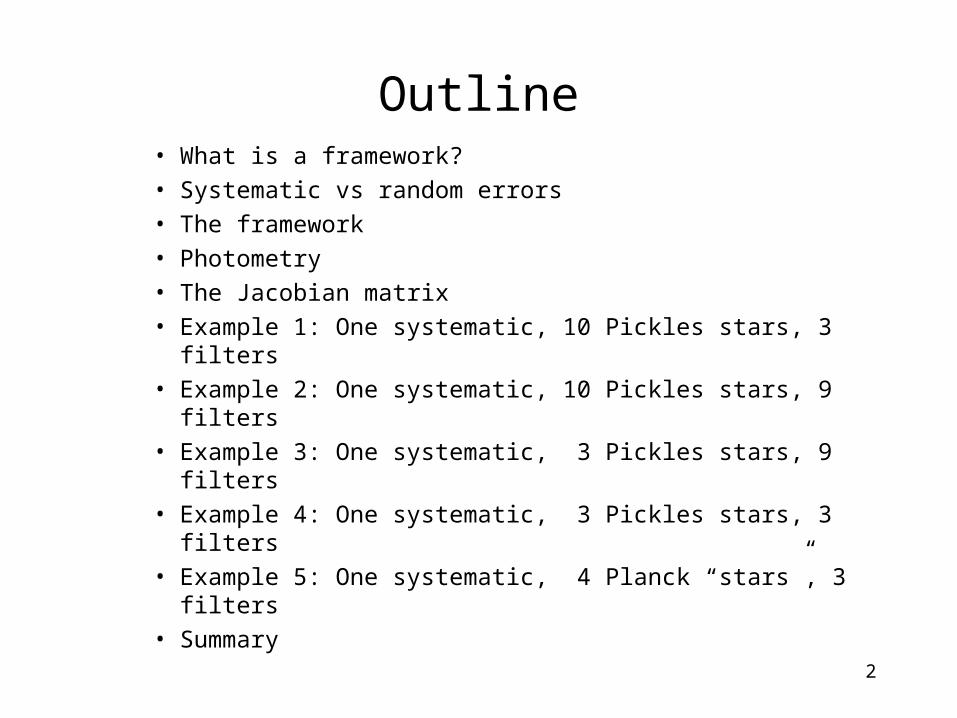
Outline• What is a framework?

• Systematic vs random errors

• The framework

• Photometry

• The Jacobian matrix

• Example 1: One systematic, 10 Pickles stars, 3 filters




• Example 5: One systematic, 4 Planck “stars”, 3 filters

• Summary

3

What is a framework?• Group closely related objectives

• Common descriptors & nomenclature

• Verifiable routines & algorithms

• Facilitates frequent discussions, interactions

• Accommodate astronomer vs physicist views

• Common open-source code where possible– Sim team is adopting Java

– Production team might use Java

• Common test cases for understandable results– Numbers alone is not enough

– Explanations should show obvious limit cases

4

Systematic Error• Each photometric measurement has a random error specific to that

datum, that perturbs the otherwise perfect agreement between data points and model points.

• In addition if the calibration star models are all too blue (or too NIR-deficient, etc)… for whatever reason… that will systematically corrupt our SEDs. Unlike measurement errors, repeating won’t help.

• Parameterizing this overall slope, curvature, etc is a way to describe our systematic SED error.

• Having got one or more parameters for this overall deviation of model SED from true SED, we can proceed to use the Fisher matrix formulism to address the corresponding errors in the cal star photometry, the filter parameters themselves, and in the target supernova photometry.

5

Schematic of a single-filter param fit w/ systematics

compare parms; histograms etc

Systematic error: all too blue, for example

6

Example:parameterization of systematics

• Cannot use simple photometric error terms in model-vs-data space (dark current, read noise, shot noise) to quantify these! Systematics are not simple random deviations in the individual data.

• Instead, need to estimate systematic error magnitude from causes outside simple photometry: WD atmospheres, NIST cal transfers, photodiode stability….

• However, if we can estimate systematic errors in model-vs-data space, then systematic parameters can be handled within the Fisher matrix formulism – and this way we get their covariances with other photometric parameters.

)1(FF 33

221model ppptrue

7

Stellar model spectra with a systematic errorred: -3%/micron

blue: +3% per micronTruth is probably among these... but not exactly known!

8

The framework• Some parameters describe systematics

– Constraint will be some data and estimated data errors from somewhere

• Some parameters describe instrument– Constraint will be data and estimated data errors from lab, orbit, ...

• Group all these parameters into a big parameter vector p[j]• Group all constraining data together into a big data vector d[i]

– These data will have an associated RMS error vector e[i]

• Compare these data against a model vector f[i] – Each f[i] will contain both systematic and instrument-related factors. – Each f[i] will often be a photometry integral over wavelength– Each f[i] will depend on some of the parameters p[j].

• Evaluate the Jacobian matrix of partial derivatives J[i,j]=df[i]/dp[j]• Evaluate the Fisher matrix F[j,k] = W[i]J[i,j] J[i,k]

– here, W[i]=weight of each datum = 1/e²[i] • Evaluate the covariance matrix C[j,k] = inverse(F[j,k]).

9

The mathematical foundation

“The Cramer-Rao inequality states that no unbiasedmethod can measure the i-th parameter with standarddeviation less than 1/√Fii if other parameters are known,nor less than √(F-1)ii if other parameters are estimatedfrom the data as well.”

Kendall, M.G. & Stuart, A. 1969, The Advanced Theory of Statistics, Volume II, Griffin, London

10

What the framework is *not*

• Not Monte Carlo: no random numbers, no exploration of nonlinearities or outliers. The framework is fully deterministic: partial derivatives of known functions. You always get the same answer.

• Not a way to do photometry. Details of exposure, dither, pixel weighting, adding background, foreground, host galaxy etc properly belong in the exposure time calculators, not here.

• Not a treatment of data. To see this, look at

We see that the Fisher matrix involves only the right hand term f/e and not the left hand term d/e. But f/e is just the model SNR, and its derivatives are just the derivatives of the model SNR. The Fisher matrix does not involve the data.

2

1

2

][

][][

NDAT

i ie

ifid

11

Photometry with systematic errors

• Photometry is an integral over wavelength

• But --- stellar models share a common systematic deviation from truth

double sum = 0.0;

for (int nm=0; nm<NWAVES; nm++)

{

double microns = 0.001 * nm;

sum += spectra[istar][nm] * systematic(microns, p) * filter(microns, tp);

}

return sum;

the stellar model’s photon flux

systematic discrepancy function ≈ 1.00

filter( ) contains instrument wavelength dependences

12

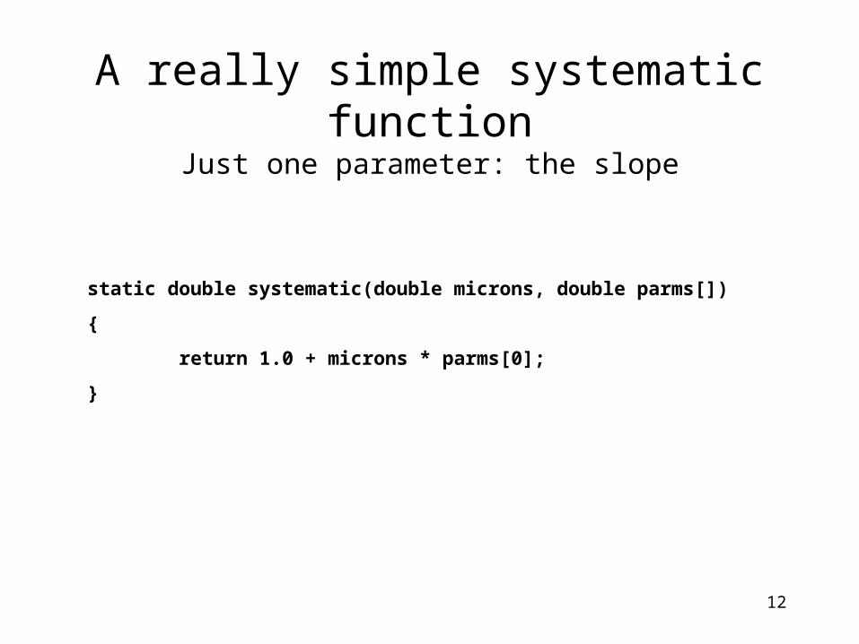
A really simple systematic functionJust one parameter: the slope

static double systematic(double microns, double parms[])

{

return 1.0 + microns * parms[0];

}

13

Getting each element of the Jacobian

• Each Jacobian element is merely a partial derivative: the sensitivity of model “i” to parameter “j” ...

double pminus[] = new double[NPARMS];

double pplus[] = new double[NPARMS];

for (int j=0; j<NPARMS; j++)

pminus[j] = pplus[j] = p[j];

int jparm = which[col];

pminus[jparm] -= DELTAP;

pplus[jparm] += DELTAP;

return (f(row, pplus) - f(row, pminus))/(2.0*DELTAP);

two-sided finite difference makes two calls to the photometry integrating routine f( )

14

Example #1

Source code is at http://www.ssl.berkeley.edu/~mlampton “Framework.java” • One systematic parameter: slope. 1%/um RMS

• Three filters: 0.42, 1.00, 1.40 microns

– Three filter parameters each: throughput, center, width

• Ten Pickles stars

• Every filter sees every star

• Signal to noise ratio = 100 everywhere– photometry signals=100; rms error=sigma[i]= 1.0 everywhere

• This is a highly overdetermined system

– 31 data points: one sys, 10x3 photometric

– 10 parameters: one sys, 9 photometric

– data far outnumber parameters => overdetermined

• Jacobian is therefore 31x10

• Fisher will be 10x10

• Covariance will be 10x10

http://www.ssl.berkeley.edu/~mlampton

15

Jacobian matrix at true parms:

Sys Thru Peak Width Thru Peak Width Thru Peak Width

SYSTEMATIC 100 0 0 0 0 0 0 0 0 0

UKO5V.DAT 43 100 -727 -86 0 0 0 0 0 0

UKB9V.DAT 44 100 -161 -142 0 0 0 0 0 0

UKA7V.DAT 44 100 143 -118 0 0 0 0 0 0

UKF5V.DAT 45 100 341 -26 0 0 0 0 0 0

UKK0III.DAT 45 100 1081 114 0 0 0 0 0 0

UKK5III.DAT 46 100 1546 335 0 0 0 0 0 0

UKK7V.DAT 46 100 1334 256 0 0 0 0 0 0

UKM2V.DAT 46 100 1339 322 0 0 0 0 0 0

UKM5III.DAT 46 100 1237 312 0 0 0 0 0 0

UKM7III.DAT 45 100 646 285 0 0 0 0 0 0

UKO5V.DAT 103 0 0 0 100 -291 -39 0 0 0

UKB9V.DAT 104 0 0 0 100 -245 -39 0 0 0

UKA7V.DAT 104 0 0 0 100 -182 -46 0 0 0

UKF5V.DAT 104 0 0 0 100 -152 -26 0 0 0

UKK0III.DAT 105 0 0 0 100 -66 -16 0 0 0

UKK5III.DAT 105 0 0 0 100 12 -6 0 0 0

UKK7V.DAT 105 0 0 0 100 -67 -24 0 0 0

UKM2V.DAT 105 0 0 0 100 13 -8 0 0 0

UKM5III.DAT 106 0 0 0 100 94 3 0 0 0

UKM7III.DAT 107 0 0 0 100 252 26 0 0 0

UKO5V.DAT 144 0 0 0 0 0 0 100 -243 -16

UKB9V.DAT 145 0 0 0 0 0 0 100 -182 -6

UKA7V.DAT 146 0 0 0 0 0 0 100 -155 1

UKF5V.DAT 146 0 0 0 0 0 0 100 -141 -21

UKK0III.DAT 147 0 0 0 0 0 0 100 -75 -18

UKK5III.DAT 147 0 0 0 0 0 0 100 -26 -5

UKK7V.DAT 147 0 0 0 0 0 0 100 -52 -13

UKM2V.DAT 147 0 0 0 0 0 0 100 -40 -11

UKM5III.DAT 148 0 0 0 0 0 0 100 27 4

UKM7III.DAT 149 0 0 0 0 0 0 100 48 16

Example 1Jacobian

Fit Model i=0…30

Parameters j=0…9

0.42um filter

1.0 um filter

1.4um filter

16



SYSTEMATIC 100 0 0 0 0 0 0 0 0 0

UKO5V.DAT 43 100 -727 -86 0 0 0 0 0 0

UKB9V.DAT 44 100 -161 -142 0 0 0 0 0 0

UKA7V.DAT 44 100 143 -118 0 0 0 0 0 0

UKF5V.DAT 45 100 341 -26 0 0 0 0 0 0

UKK0III.DAT 45 100 1081 114 0 0 0 0 0 0

UKK5III.DAT 46 100 1546 335 0 0 0 0 0 0

UKK7V.DAT 46 100 1334 256 0 0 0 0 0 0

UKM2V.DAT 46 100 1339 322 0 0 0 0 0 0

UKM5III.DAT 46 100 1237 312 0 0 0 0 0 0

UKM7III.DAT 45 100 646 285 0 0 0 0 0 0

UKO5V.DAT 103 0 0 0 100 -291 -39 0 0 0

UKB9V.DAT 104 0 0 0 100 -245 -39 0 0 0

UKA7V.DAT 104 0 0 0 100 -182 -46 0 0 0

UKF5V.DAT 104 0 0 0 100 -152 -26 0 0 0

UKK0III.DAT 105 0 0 0 100 -66 -16 0 0 0

UKK5III.DAT 105 0 0 0 100 12 -6 0 0 0

UKK7V.DAT 105 0 0 0 100 -67 -24 0 0 0

UKM2V.DAT 105 0 0 0 100 13 -8 0 0 0

UKM5III.DAT 106 0 0 0 100 94 3 0 0 0

UKM7III.DAT 107 0 0 0 100 252 26 0 0 0

UKO5V.DAT 144 0 0 0 0 0 0 100 -243 -16

UKB9V.DAT 145 0 0 0 0 0 0 100 -182 -6

UKA7V.DAT 146 0 0 0 0 0 0 100 -155 1

UKF5V.DAT 146 0 0 0 0 0 0 100 -141 -21

UKK0III.DAT 147 0 0 0 0 0 0 100 -75 -18

UKK5III.DAT 147 0 0 0 0 0 0 100 -26 -5

UKK7V.DAT 147 0 0 0 0 0 0 100 -52 -13

UKM2V.DAT 147 0 0 0 0 0 0 100 -40 -11

UKM5III.DAT 148 0 0 0 0 0 0 100 27 4

UKM7III.DAT 149 0 0 0 0 0 0 100 48 16

Jacobian, cont’d

These come out around 146 because at 1.4+ microns, a unit rise in the systematic slope (integrated over the stellar continuum and filter) gives a 146 sigma rise in these model data.

This is 100 by choice: a unit shift in systematic slope gives a 100 sigma departure from the best fit model.

These are 100 by choice: a unit shift in throughput gives a 100 sigma departure from the best fit model.

17

Example 1Fisher

Fisher matrix at true parms:

355025 44970 311479 57771 104848 -64506 -18158 146573 -121707 -10151

44970 100000 678032 125058 0 0 0 0 0 0

311479 678032 9773919 2043362 0 0 0 0 0 0

57771 125058 2043362 515151 0 0 0 0 0 0

104848 0 0 0 100000 -63086 -17522 0 0 0

-64506 0 0 0 -63086 282031 42422 0 0 0

-18158 0 0 0 -17522 42422 7429 0 0 0

146573 0 0 0 0 0 0 100000 -83769 -6984

-121707 0 0 0 0 0 0 -83769 149577 11322

-10151 0 0 0 0 0 0 -6984 11322 1684

2

0

1 weight where

],[],[][],[

i

NDAT

i

/σ W[i]

kiJjiJiWkjF

In this example I’ve chosen to study SNR=100, and have chosen all the photometry signals to come out=100 for the nominal parameters; and therefore choose all the W[i]=1.0

10 independent data (SNR=100) ² = 100000

18

Example 1Covariance and RMS

Covariance matrix at true parms:

1.00E-4 -4.41E-5 -1.22E-7 -1.96E-8 -1.05E-4 -6.10E-7 -5.08E-7 -1.48E-4 -1.26E-6 -1.34E-6

-4.41E-5 3.95E-5 -2.14E-6 3.82E-6 4.65E-5 2.69E-7 2.24E-7 6.52E-5 5.57E-7 5.92E-7

-1.22E-7 -2.14E-6 8.38E-7 -2.79E-6 1.29E-7 7.47E-10 6.21E-10 1.81E-7 1.55E-9 1.64E-9

-1.96E-8 3.82E-6 -2.79E-6 1.21E-5 2.06E-8 1.19E-10 9.93E-11 2.89E-8 2.47E-10 2.62E-10

-1.05E-4 4.65E-5 1.29E-7 2.06E-8 1.52E-4 -3.75E-5 3.16E-4 1.56E-4 1.33E-6 1.41E-6

-6.10E-7 2.69E-7 7.47E-10 1.19E-10 -3.75E-5 6.06E-5 -4.36E-4 9.02E-7 7.71E-9 8.19E-9

-5.08E-7 2.24E-7 6.21E-10 9.93E-11 3.16E-4 -4.36E-4 3.37E-3 7.50E-7 6.41E-9 6.81E-9

-1.48E-4 6.52E-5 1.81E-7 2.89E-8 1.56E-4 9.02E-7 7.50E-7 2.37E-4 1.14E-5 1.68E-5

-1.26E-6 5.57E-7 1.55E-9 2.47E-10 1.33E-6 7.71E-9 6.41E-9 1.14E-5 1.84E-5 -8.41E-5

-1.34E-6 5.92E-7 1.64E-9 2.62E-10 1.41E-6 8.19E-9 6.81E-9 1.68E-5 -8.41E-5 1.22E-3

RMS absolute parameter errors = sqrt(cov[i,i])...

0.0100 0.0063 0.0009 0.0035 0.0123 0.0078 0.0580 0.0154 0.0043 0.0349

],[][

]),[(],[

kkCovkRMSparam

kjFisherinversekjCov

1% systematic, by fiat

precise in B band! Less precise in NIR

19

Exploring Example #1

• Suppose we somehow boost the accuracy of the systematic parameter so that its error is only 0.01% – Manually raise the value of J[0,0] to 10000, keeping RMS

error=1

– the rest of the Jacobian matrix is of course unaffected

– Fisher matrix values are unaffected except for F[0,0] which becomes enormous;

– Covariance matrix values are made smaller, especially C[0,0] which becomes 1E-8;

– Parameter errors are reduced, hugely for p[0]=systematic, but also for the filter throughput parameters. This shows the benefit of better control over systematics. Band centers and widths are not aided.

20

Exploring Example #1, continued

• Or..what happens if we enlarge the systematic error, seeking to explore 4%/micron RMS? – Make J[0,0]=25 with sigma again kept = 1.0;

– the rest of the Jacobian matrix is of course unaffected;

– only F[0,0] of the Fisher matrix is reduced;

– the covariance matrix elements grow. A lot!

– the filter throughput parameter uncertainties grow. A lot!

summary: for J[0,0] = 100, 10000, and 25...

sys thru0 cent0 width0 thru1 cent1 width1 thru2 cent2 width2

0.0100 0.0063 0.0009 0.0035 0.0123 0.0078 0.0580 0.0154 0.0043 0.0349

0.0001 0.0045 0.0009 0.0035 0.0064 0.0078 0.0580 0.0044 0.0043 0.0349

0.0400 0.0182 0.0009 0.0035 0.0426 0.0078 0.0580 0.0592 0.0043 0.0349

21

Adding information• Preceding examples show that fooling with the Jacobian’s

systematic constraint flows straight through to all the relevant filter parameters (assumed here to be constrained only by photometry).

• Actually, the Fisher matrix (a.k.a. information matrix) is an ideal receptacle for adding information. If you know something extra about parameter p[j] independent of the other parameters, go ahead and add a term to F[j,j]. The term should be SNR², for example 1E6 if the new information constrains the observation to 0.1% relative accuracy.

• Extreme case: given that some parameter is exactly known, don’t try to add infinity to F[j,j] --- instead, delete row j and column j before inverting to obtain the covariance. Parameter j will no longer contribute to the joint parameter errors.

22

Extra information for Example #1

• Suppose filter centers and widths are known to be ultra stable from preflight testing. Let’s say 0.1% rms.

• Add +1E6 to F[2,2], F[3,3] F[5,5], F[6,6], F[8,8], and F[9,9].

• Proceed to invert...and get:

• This act reduces the RMS error of each center and width to a tiny value, less than 0.001, and furthermore the overall throughput errors become simply the RSS of the 1%/micron slope systematic and the 0.316% error from ten independent 1% photometry calibrations.



0.0100 0.0061 0.0004 0.0009 0.0110 0.0009 0.0010 0.0150 0.0010 0.0010

23

More extreme: perfect knowledge of centers and widths of all filters in Example #1

• Drop rows 2,3,5,6,8,9 from Fisher

• Drop cols 2,3,5,6,8,9 from Fisher

• Instead of 10x10, have 4x4

• Invert Fisher to get the resulting covariance

• Result: the systematic now dominates everything – as it should, given ten stars but only one systematic determination, each at 100:1


3.6E5 44970 104848 146573

44970 100000 0 0

104848 0 100000 0

146573 0 0 100000


1.0E-4 -4.5E-5 -1.0E-4 -1.5E-4

-4.5E-5 3.0E-5 4.7E-5 6.6E-5

-1.0E-4 4.7E-5 1.2E-4 1.5E-4

-1.5E-4 6.6E-5 1.5E-4 2.2E-4


0.0100 0.0055 0.0109 0.0150

24

Example #2

• Nine filters– throughput is the only active parameter– other filter parameters are assumed perfectly known

• Ten stars– each observation has SNR = 100:1

• One systematic– overall slope, 1% uncertainty

• Jacobian will be 91 x 10– system is strongly overdetermined

• Fisher will be 10 x 10• Covariance will be 10 x 10

25

Example #2 results


694988 44871 51127 58692 67819 77613 88899 101775 116543 133971

44871 100000 0 0 0 0 0 0 0 0

51127 0 100000 0 0 0 0 0 0 0

58692 0 0 100000 0 0 0 0 0 0

67819 0 0 0 100000 0 0 0 0 0

77613 0 0 0 0 100000 0 0 0 0

88899 0 0 0 0 0 100000 0 0 0

101775 0 0 0 0 0 0 100000 0 0

116543 0 0 0 0 0 0 0 100000 0

133971 0 0 0 0 0 0 0 0 100000

26

Example #2 results continued


9.9E-5 -4.4E-5 -5.1E-5 -5.8E-5 -6.7E-5 -7.7E-5 -8.8E-5 -1.0E-4 -1.2E-4 -1.3E-4

-4.4E-5 3.0E-5 2.3E-5 2.6E-5 3.0E-5 3.4E-5 3.9E-5 4.5E-5 5.2E-5 5.9E-5

-5.1E-5 2.3E-5 3.6E-5 3.0E-5 3.4E-5 3.9E-5 4.5E-5 5.1E-5 5.9E-5 6.8E-5

-5.8E-5 2.6E-5 3.0E-5 4.4E-5 3.9E-5 4.5E-5 5.2E-5 5.9E-5 6.8E-5 7.8E-5

-6.7E-5 3.0E-5 3.4E-5 3.9E-5 5.5E-5 5.2E-5 6.0E-5 6.8E-5 7.8E-5 9.0E-5

-7.7E-5 3.4E-5 3.9E-5 4.5E-5 5.2E-5 7.0E-5 6.8E-5 7.8E-5 8.9E-5 1.0E-4

-8.8E-5 3.9E-5 4.5E-5 5.2E-5 6.0E-5 6.8E-5 8.8E-5 8.9E-5 1.0E-4 1.2E-4

-1.0E-4 4.5E-5 5.1E-5 5.9E-5 6.8E-5 7.8E-5 8.9E-5 1.1E-4 1.2E-4 1.3E-4

-1.2E-4 5.2E-5 5.9E-5 6.8E-5 7.8E-5 8.9E-5 1.0E-4 1.2E-4 1.4E-4 1.5E-4

-1.3E-4 5.9E-5 6.8E-5 7.8E-5 9.0E-5 1.0E-4 1.2E-4 1.3E-4 1.5E-4 1.9E-4


0.0099 0.0055 0.0060 0.0066 0.0074 0.0083 0.0094 0.0106 0.0120 0.0137

27

Example #3

• Nine filters– throughput is the only active parameter– other filter parameters are assumed perfectly known

• Three stars: late M7, K0, O5 (all Pickles)– each observation has SNR = 100:1

• One systematic– overall slope, 1% uncertainty

• Jacobian will be 28 x 10– system is somewhat overdetermined


28

Example #3 results:

Jacobian



SYSTEMATIC 100 0 0 0 0 0 0 0 0 0

UKO5V.DAT 43 100 0 0 0 0 0 0 0 0

UKK0III.DAT 45 100 0 0 0 0 0 0 0 0

UKM7III.DAT 45 100 0 0 0 0 0 0 0 0

UKO5V.DAT 50 0 100 0 0 0 0 0 0 0

UKK0III.DAT 51 0 100 0 0 0 0 0 0 0

UKM7III.DAT 52 0 100 0 0 0 0 0 0 0

UKO5V.DAT 57 0 0 100 0 0 0 0 0 0

UKK0III.DAT 59 0 0 100 0 0 0 0 0 0

UKM7III.DAT 60 0 0 100 0 0 0 0 0 0

UKO5V.DAT 66 0 0 0 100 0 0 0 0 0

UKK0III.DAT 67 0 0 0 100 0 0 0 0 0

UKM7III.DAT 71 0 0 0 100 0 0 0 0 0

UKO5V.DAT 76 0 0 0 0 100 0 0 0 0

UKK0III.DAT 77 0 0 0 0 100 0 0 0 0

UKM7III.DAT 81 0 0 0 0 100 0 0 0 0

UKO5V.DAT 87 0 0 0 0 0 100 0 0 0

UKK0III.DAT 88 0 0 0 0 0 100 0 0 0

UKM7III.DAT 92 0 0 0 0 0 100 0 0 0

UKO5V.DAT 100 0 0 0 0 0 0 100 0 0

UKK0III.DAT 102 0 0 0 0 0 0 100 0 0

UKM7III.DAT 104 0 0 0 0 0 0 100 0 0

UKO5V.DAT 115 0 0 0 0 0 0 0 100 0

UKK0III.DAT 117 0 0 0 0 0 0 0 100 0

UKM7III.DAT 118 0 0 0 0 0 0 0 100 0

UKO5V.DAT 132 0 0 0 0 0 0 0 0 100

UKK0III.DAT 134 0 0 0 0 0 0 0 0 100

UKM7III.DAT 135 0 0 0 0 0 0 0 0 100

29

Example #3 results: Fisher


216050 13333 15277 17599 20469 23387 26776 30601 34997 40182

13333 30000 0 0 0 0 0 0 0 0

15277 0 30000 0 0 0 0 0 0 0

17599 0 0 30000 0 0 0 0 0 0

20469 0 0 0 30000 0 0 0 0 0

23387 0 0 0 0 30000 0 0 0 0

26776 0 0 0 0 0 30000 0 0 0

30601 0 0 0 0 0 0 30000 0 0

34997 0 0 0 0 0 0 0 30000 0

40182 0 0 0 0 0 0 0 0 30000

30

Example #3 results: Covariance


9.9E-5 -4.4E-5 -5.1E-5 -5.8E-5 -6.8E-5 -7.7E-5 -8.9E-5 -1.0E-4 -1.2E-4 -1.3E-4

-4.4E-5 5.3E-5 2.2E-5 2.6E-5 3.0E-5 3.4E-5 3.9E-5 4.5E-5 5.2E-5 5.9E-5

-5.1E-5 2.2E-5 5.9E-5 3.0E-5 3.5E-5 3.9E-5 4.5E-5 5.2E-5 5.9E-5 6.8E-5

-5.8E-5 2.6E-5 3.0E-5 6.8E-5 4.0E-5 4.5E-5 5.2E-5 5.9E-5 6.8E-5 7.8E-5

-6.8E-5 3.0E-5 3.5E-5 4.0E-5 8.0E-5 5.3E-5 6.1E-5 6.9E-5 7.9E-5 9.1E-5

-7.7E-5 3.4E-5 3.9E-5 4.5E-5 5.3E-5 9.4E-5 6.9E-5 7.9E-5 9.0E-5 1.0E-4

-8.9E-5 3.9E-5 4.5E-5 5.2E-5 6.1E-5 6.9E-5 1.1E-4 9.0E-5 1.0E-4 1.2E-4

-1.0E-4 4.5E-5 5.2E-5 5.9E-5 6.9E-5 7.9E-5 9.0E-5 1.4E-4 1.2E-4 1.4E-4

-1.2E-4 5.2E-5 5.9E-5 6.8E-5 7.9E-5 9.0E-5 1.0E-4 1.2E-4 1.7E-4 1.6E-4

-1.3E-4 5.9E-5 6.8E-5 7.8E-5 9.1E-5 1.0E-4 1.2E-4 1.4E-4 1.6E-4 2.1E-4


0.0100 0.0073 0.0077 0.0082 0.0089 0.0097 0.0106 0.0117 0.0130 0.0145

31

Example #4

• Three filters: 0.42, 1.0, 1.4 microns – three active parameters per filter: throughput,

center, and width• Three stars: late M7, K0, O5 (all Pickles)

– each observation has SNR = 100:1• One systematic

– overall slope, 1% uncertainty• Jacobian will be 10 x 10

– system is barely determined


32

Example #4 results: Jacobian



SYSTEMATIC 100 0 0 0 0 0 0 0 0 0

UKO5V.DAT 43 100 -727 -86 0 0 0 0 0 0

UKK0III.DAT 45 100 1081 114 0 0 0 0 0 0

UKM7III.DAT 45 100 646 285 0 0 0 0 0 0

UKO5V.DAT 103 0 0 0 100 -291 -39 0 0 0

UKK0III.DAT 105 0 0 0 100 -66 -16 0 0 0

UKM7III.DAT 107 0 0 0 100 252 26 0 0 0

UKO5V.DAT 144 0 0 0 0 0 0 100 -243 -16

UKK0III.DAT 147 0 0 0 0 0 0 100 -75 -18

UKM7III.DAT 149 0 0 0 0 0 0 100 48 16

33



113493 13360 46511 14202 31521 -10021 -2946 43957 -38863 -2632

13360 30000 99934 31266 0 0 0 0 0 0

46511 99934 2114349 369727 0 0 0 0 0 0

14202 31266 369727 101620 0 0 0 0 0 0

31521 0 0 0 30000 -10491 -2918 0 0 0

-10021 0 0 0 -10491 152424 18785 0 0 0

-2946 0 0 0 -2918 18785 2418 0 0 0

43957 0 0 0 0 0 0 30000 -26931 -1842

-38863 0 0 0 0 0 0 -26931 66828 6078

-2632 0 0 0 0 0 0 -1842 6078 861

34

Example #4 results: CovarianceCovariance matrix at true parms:

1.0E-4 -4.4E-5 -1.2E-7 7.1E-8 -1.1E-4 -4.8E-7 -1.7E-6 -1.5E-4 -1.3E-6 -1.4E-6

-4.4E-5 6.9E-5 9.5E-7 -1.9E-5 4.7E-5 2.1E-7 7.4E-7 6.5E-5 5.6E-7 6.0E-7

-1.2E-7 9.5E-7 1.3E-6 -5.1E-6 1.3E-7 5.9E-10 2.1E-9 1.8E-7 1.6E-9 1.7E-9

7.1E-8 -1.9E-5 -5.1E-6 3.4E-5 -7.5E-8-3.4E-10 -1.2E-9 -1.0E-7-8.9E-10-9.6E-10

-1.1E-4 4.7E-5 1.3E-7 -7.5E-8 3.8E-4 -5.1E-4 4.3E-3 1.6E-4 1.3E-6 1.4E-6

-4.8E-7 2.1E-7 5.9E-10-3.4E-10 -5.1E-4 1.1E-3 -9.2E-3 7.0E-7 6.0E-9 6.5E-9

-1.7E-6 7.4E-7 2.1E-9 -1.2E-9 4.3E-3 -9.2E-3 7.7E-2 2.5E-6 2.1E-8 2.3E-8

-1.5E-4 6.5E-5 1.8E-7 -1.0E-7 1.6E-4 7.0E-7 2.5E-6 2.7E-4 3.4E-5 -1.1E-4

-1.3E-6 5.6E-7 1.6E-9-8.9E-10 1.3E-6 6.0E-9 2.1E-8 3.4E-5 6.1E-5 -3.6E-4

-1.4E-6 6.0E-7 1.7E-9-9.6E-10 1.4E-6 6.5E-9 2.3E-8 -1.1E-4 -3.6E-4 3.5E-3



0.0100 0.0083 0.0011 0.0058 0.0196 0.0333 0.2781 0.0166 0.0078 0.0588

poor determination of widths

35

Example #5

• Three filters: 0.42, 1.0, 1.4 microns – three active parameters per filter: throughput,

center, and width• Four Planck “stars”: 3000, 5000, 10000, 80000K

– each observation has SNR = 100:1• One systematic

– overall slope, 1% uncertainty• Jacobian will be 13 x 10

– system is barely determined


36

Example #5 results: JacobianJacobian matrix at true parms:


SYSTEMATIC 100 0 0 0 0 0 0 0 0 0

3000 46 100 1412 499 0 0 0 0 0 0

5000 45 100 536 111 0 0 0 0 0 0

10000 44 100 -161 -42 0 0 0 0 0 0

80000 43 100 -678 -81 0 0 0 0 0 0

3000 106 0 0 0 100 49 1 0 0 0

5000 105 0 0 0 100 -112 -23 0 0 0

10000 104 0 0 0 100 -221 -31 0 0 0

80000 103 0 0 0 100 -298 -34 0 0 0

3000 147 0 0 0 0 0 0 100 -48 -13

5000 146 0 0 0 0 0 0 100 -126 -20

10000 145 0 0 0 0 0 0 100 -177 -23

80000 145 0 0 0 0 0 0 100 -214 -24

37



146339 17831 52560 22625 41728 -60303 -8951 58258 -82127 -11558

17831 40000 110952 48774 0 0 0 0 0 0

52560 110952 2766359 825656 0 0 0 0 0 0

22625 48774 825656 269819 0 0 0 0 0 0

41728 0 0 0 40000 -58237 -8625 0 0 0

-60303 0 0 0 -58237 152787 19567 0 0 0

-8951 0 0 0 -8625 19567 2629 0 0 0

58258 0 0 0 0 0 0 40000 -56530 -7945

-82127 0 0 0 0 0 0 -56530 95474 12276

-11558 0 0 0 0 0 0 -7945 12276 1653

38

Example #5 results: CovarianceCovariance matrix at true parms:

1.0E-4 -4.4E-5 -1.1E-7 -7.0E-8 -1.1E-4 -6.0E-7 -5.8E-7 -1.5E-4 -1.2E-6 -1.3E-6

-4.4E-5 5.9E-5 6.4E-6 -2.7E-5 4.7E-5 2.7E-7 2.6E-7 6.5E-5 5.5E-7 5.7E-7

-1.1E-7 6.4E-6 5.2E-6 -1.7E-5 1.1E-7 6.4E-10 6.2E-10 1.6E-7 1.3E-9 1.4E-9

-7.0E-8 -2.7E-5 -1.7E-5 6.1E-5 7.3E-8 4.2E-10 4.1E-10 1.0E-7 8.6E-10 8.9E-10

-1.1E-4 4.7E-5 1.1E-7 7.3E-8 2.6E-4 -1.2E-4 1.4E-3 1.6E-4 1.3E-6 1.3E-6

-6.0E-7 2.7E-7 6.4E-10 4.2E-10 -1.2E-4 2.4E-4 -2.2E-3 8.9E-7 7.4E-9 7.7E-9

-5.8E-7 2.6E-7 6.2E-10 4.1E-10 1.4E-3 -2.2E-3 2.1E-2 8.6E-7 7.2E-9 7.5E-9

-1.5E-4 6.5E-5 1.6E-7 1.0E-7 1.6E-4 8.9E-7 8.6E-7 2.9E-3 -1.5E-3 2.4E-2

-1.2E-6 5.5E-7 1.3E-9 8.6E-10 1.3E-6 7.4E-9 7.2E-9 -1.5E-3 1.1E-3 -1.6E-2

-1.3E-6 5.7E-7 1.4E-9 8.9E-10 1.3E-6 7.7E-9 7.5E-9 2.4E-2 -1.6E-2 2.3E-1



0.0100 0.0077 0.0023 0.0078 0.0161 0.0156 0.1463 0.0538 0.0335 0.4847

poor determination of NIR widthsgood in the visible!

39

Summary

• The proposed framework has three ways to incorporate added information:

– augmenting the relevant Jacobian element

– augmenting the Fisher matrix diagonal element

– dropping row & column of Fisher

• The proposed framework has some explanatory power

• The proposed framework can be implemented in an open-source Java environment

40

further reading...• Press et al “Numerical Recipes in C, 2nd edition”

– Fisher matrix alpha eqn 15.5.11– covariance matrix eqn 15.5.15– confidence limits sec 15.6

• Data Reduction and Error Analysis for the Physical Sciences, P.R.Bevington and D.K.Robinson, 3rd edition, McGraw Hill, 2002

• Data Analysis: A Bayesian Tutorial, D.S.Silva, Clarendon Press, Oxford, 1996• Wayne Hu’s tutorial on the subject, including Cramer-Rao bound and the

connection between Fisher and the curvature of the log likelihood function: http://background.uchicago.edu/~whu/Courses/Ast448_02/notes7w.pdf

• Ed Dowski, U.Colo, http://www.colorado.edu/isl/papers/info/node2.html• Don Johnson, Rice U., http://cnx.rice.edu/content/m11266/latest/#Cramer• H. Cramér. (1946). Mathematical Methods of Statistics. Princeton, NJ:

Princeton University Press • Tegmark et al, astro-ph/9804168

http://www.colorado.edu/isl/papers/info/node2.html

http://cnx.rice.edu/content/m11266/latest/#Cramer

1 Fisher Matrix Framework for Photometric Error Estimation M.Lampton Space Sciences Lab U.C.Berkeley...

Documents

Transcript of 1 Fisher Matrix Framework for Photometric Error Estimation M.Lampton Space Sciences Lab U.C.Berkeley...